chapter 5dpuadweb.depauw.edu/.../etextproject/ac2.1files/chapter5.pdf · 2016-06-02 · chapter 5...
TRANSCRIPT
147
Chapter 5
Standardizing Analytical Methods
Chapter Overview5A Analytical Standards5B Calibrating the Signal (Stotal)5C Determining the Sensitivity (kA)5D Linear Regression and Calibration Curves5E Compensating for the Reagent Blank (Sreag)5F Using Excel and R for a Regression Analysis5G Key Terms5H Chapter Summary5I Problems5J Solutions to Practice Exercises
The American Chemical Society’s Committee on Environmental Improvement defines standardization as the process of determining the relationship between the signal and the amount of analyte in a sample.1 In Chapter 3 we defined this relationship as
S k n S S k Cortotal A A reag total A A= + =
where Stotal is the signal, nA is the moles of analyte, CA is the analyte’s concentration, kA is the method’s sensitivity for the analyte, and Sreag is the contribution to Stotal from sources other than the sample. To standardize a method we must determine values for kA and Sreag. Strategies for accomplishing this are the subject of this chapter.
1 ACS Committee on Environmental Improvement “Guidelines for Data Acquisition and Data Quality Evaluation in Environmental Chemistry,” Anal. Chem. 1980, 52, 2242–2249.

148 Analytical Chemistry 2.1
5A Analytical StandardsTo standardize an analytical method we use standards that contain known amounts of analyte. The accuracy of a standardization, therefore, depends on the quality of the reagents and the glassware we use to prepare these standards. For example, in an acid–base titration the stoichiometry of the acid–base reaction defines the relationship between the moles of analyte and the moles of titrant. In turn, the moles of titrant is the product of the titrant’s concentration and the volume of titrant used to reach the equiva-lence point. The accuracy of a titrimetric analysis, therefore, is never better than the accuracy with which we know the titrant’s concentration.
5A.1 Primary and Secondary Standards
There are two categories of analytical standards: primary standards and sec-ondary standards. A primary standard is a reagent that we can use to dispense an accurately known amount of analyte. For example, a 0.1250-g sample of K2Cr2O7 contains 4.249 × 10⁻⁴ moles of K2Cr2O7. If we place this sample in a 250-mL volumetric flask and dilute to volume, the concen-tration of K2Cr2O7 in the resulting solution is 1.700 × 10⁻³ M. A primary standard must have a known stoichiometry, a known purity (or assay), and it must be stable during long-term storage. Because it is difficult to estab-lishing accurately the degree of hydration, even after drying, a hydrated reagent usually is not a primary standard.
Reagents that do not meet these criteria are secondary standards. The concentration of a secondary standard is determined relative to a pri-mary standard. Lists of acceptable primary standards are available.2 Appen-dix 8 provides examples of some common primary standards.
5A.2 Other Reagents
Preparing a standard often requires additional reagents that are not primary standards or secondary standards, such as a suitable solvent or reagents needed to adjust the standard’s matrix. These solvents and reagents are po-tential sources of additional analyte, which, if not accounted for, produce a determinate error in the standardization. If available, reagent grade chemicals that conform to standards set by the American Chemical Society are used.3 The label on the bottle of a reagent grade chemical (Figure 5.1) lists either the limits for specific impurities or provides an assay for the impurities. We can improve the quality of a reagent grade chemical by pu-rifying it, or by conducting a more accurate assay. As discussed later in the chapter, we can correct for contributions to Stotal from reagents used in an
2 (a) Smith, B. W.; Parsons, M. L. J. Chem. Educ. 1973, 50, 679–681; (b) Moody, J. R.; Green-burg, P. R.; Pratt, K. W.; Rains, T. C. Anal. Chem. 1988, 60, 1203A–1218A.
3 Committee on Analytical Reagents, Reagent Chemicals, 8th ed., American Chemical Society: Washington, D. C., 1993.
See Chapter 9 for a thorough discussion of titrimetric methods of analysis.
NaOH is one example of a secondary standard. Commercially available NaOH contains impurities of NaCl, Na2CO3, and Na2SO4, and readily absorbs H2O from the atmosphere. To determine the concentration of NaOH in a solution, we titrate it against a primary standard weak acid, such as potassium hydrogen phthal-ate, KHC8H4O4.

149Chapter 5 Standardizing Analytical Methods
analysis by including an appropriate blank determination in the analytical procedure.
5A.3 Preparing a Standard Solution
It often is necessary to prepare a series of standards, each with a different concentration of analyte. We can prepare these standards in two ways. If the range of concentrations is limited to one or two orders of magnitude, then each solution is best prepared by transferring a known mass or volume of the pure standard to a volumetric flask and diluting to volume.
When working with a larger range of concentrations, particularly a range that extends over more than three orders of magnitude, standards are best prepared by a serial dilution from a single stock solution. In a serial dilution we prepare the most concentrated standard and then dilute a portion of that solution to prepare the next most concentrated standard. Next, we dilute a portion of the second standard to prepare a third standard, continuing this process until we have prepared all of our standards. Serial dilutions must be prepared with extra care because an error in preparing one standard is passed on to all succeeding standards.
Figure 5.1 Two examples of packaging labels for reagent grade chemicals. The label in (a) pro-vides the manufacturer’s assay for the reagent, NaBr. Note that potassium is flagged with an asterisk (*) because its assay exceeds the limit established by the American Chemical Society (ACS). The label in (b) does not provide an assay for impurities; however it indicates that the reagent meets ACS specifications by providing the maximum limits for impurities. An assay for the reagent, NaHCO3, is provided.
(a) (b)
150 Analytical Chemistry 2.1
5B Calibrating the Signal (Stotal)The accuracy with which we determine kA and Sreag depends on how accu-rately we can measure the signal, Stotal. We measure signals using equipment, such as glassware and balances, and instrumentation, such as spectropho-tometers and pH meters. To minimize determinate errors that might affect the signal, we first calibrate our equipment and instrumentation by measur-ing Stotal for a standard with a known response of Sstd, adjusting Stotal until
S Stotal std=
Here are two examples of how we calibrate signals; other examples are pro-vided in later chapters that focus on specific analytical methods.
When the signal is a measurement of mass, we determine Stotal using an analytical balance. To calibrate the balance’s signal we use a reference weight that meets standards established by a governing agency, such as the National Institute for Standards and Technology or the American Society for Testing and Materials. An electronic balance often includes an internal calibration weight for routine calibrations, as well as programs for calibrat-ing with external weights. In either case, the balance automatically adjusts Stotal to match Sstd.
We also must calibrate our instruments. For example, we can evaluate a spectrophotometer’s accuracy by measuring the absorbance of a carefully prepared solution of 60.06 mg/L K2Cr2O7 in 0.0050 M H2SO4, using 0.0050 M H2SO4 as a reagent blank.4 An absorbance of 0.640 ± 0.010 absorbance units at a wavelength of 350.0 nm indicates that the spectrom-eter’s signal is calibrated properly.
5C Determining the Sensitivity (kA)To standardize an analytical method we also must determine the analyte’s sensitivity, kA, in equation 5.1 or equation 5.2.
S k n Stotal A A reag= + 5.1
S k C Stotal A A reag= + 5.2In principle, it is possible to derive the value of kA for any analytical method if we understand fully all the chemical reactions and physical processes re-sponsible for the signal. Unfortunately, such calculations are not feasible if we lack a sufficiently developed theoretical model of the physical processes or if the chemical reaction’s evince non-ideal behavior. In such situations we must determine the value of kA by analyzing one or more standard solutions, each of which contains a known amount of analyte. In this section we con-sider several approaches for determining the value of kA. For simplicity we assume that Sreag is accounted for by a proper reagent blank, allowing us to replace Stotal in equation 5.1 and equation 5.2 with the analyte’s signal, SA.
4 Ebel, S. Fresenius J. Anal. Chem. 1992, 342, 769.
See Section 2D.1 to review how an elec-tronic balance works. Calibrating a bal-ance is important, but it does not elimi-nate all sources of determinate error when measuring mass. See Appendix 9 for a discussion of correcting for the buoyancy of air.
Be sure to read and follow carefully the calibration instructions provided with any instrument you use.

151Chapter 5 Standardizing Analytical Methods
S k nA A A= 5.3
S k CA A A= 5.4
5C.1 Single-Point versus Multiple-Point Standardizations
The simplest way to determine the value of kA in equation 5.4 is to use a single-point standardization in which we measure the signal for a standard, Sstd, that contains a known concentration of analyte, Cstd. Substi-tuting these values into equation 5.4
k CS
Astd
std= 5.5
gives us the value for kA. Having determined kA, we can calculate the con-centration of analyte in a sample by measuring its signal, Ssamp, and calculat-ing CA using equation 5.6.
C kS
AA
samp= 5.6
A single-point standardization is the least desirable method for stan-dardizing a method. There are two reasons for this. First, any error in our determination of kA carries over into our calculation of CA. Second, our experimental value for kA is based on a single concentration of analyte. To extend this value of kA to other concentrations of analyte requires that we assume a linear relationship between the signal and the analyte’s con-centration, an assumption that often is not true.5 Figure 5.2 shows how assuming a constant value of kA leads to a determinate error in CA if kA be-comes smaller at higher concentrations of analyte. Despite these limitations, single-point standardizations find routine use when the expected range for the analyte’s concentrations is small. Under these conditions it often is safe
5 Cardone, M. J.; Palmero, P. J.; Sybrandt, L. B. Anal. Chem. 1980, 52, 1187–1191.
Equation 5.3 and equation 5.4 essentially are identical, differing only in whether we choose to express the amount of analyte in moles or as a concentration. For the re-mainder of this chapter we will limit our treatment to equation 5.4. You can extend this treatment to equation 5.3 by replac-ing CA with nA.
Figure 5.2 Example showing how a single-point standard-ization leads to a determinate error in an analyte’s reported concentration if we incorrectly assume that kA is constant. The assumed relationship between Ssamp and CA is based on a single standard and is a straight-line; the actual relationship between Ssamp and CA becomes curved for larger concentra-tions of analyte.
(CA)reportedCstd
Sstd
Ssamp
(CA)actual
actual relationship
assumed relationship
152 Analytical Chemistry 2.1
to assume that kA is constant (although you should verify this assumption experimentally). This is the case, for example, in clinical labs where many automated analyzers use only a single standard.
The better way to standardize a method is to prepare a series of standards, each of which contains a different concentration of analyte. Standards are chosen such that they bracket the expected range for the analyte’s concen-tration. A multiple-point standardization should include at least three standards, although more are preferable. A plot of Sstd versus Cstd is called a calibration curve. The exact standardization, or calibration relationship, is determined by an appropriate curve-fitting algorithm.
There are two advantages to a multiple-point standardization. First, al-though a determinate error in one standard introduces a determinate error, its effect is minimized by the remaining standards. Second, because we measure the signal for several concentrations of analyte, we no longer must assume kA is independent of the analyte’s concentration. Instead, we can construct a calibration curve similar to the “actual relationship” in Figure 5.2.
5C.2 External Standards
The most common method of standardization uses one or more external standards, each of which contains a known concentration of analyte. We call these standards “external” because they are prepared and analyzed sepa-rate from the samples.
Single external Standard
With a single external standard we determine kA using equation 5.5 and then calculate the concentration of analyte, CA, using equation 5.6.
Example 5.1
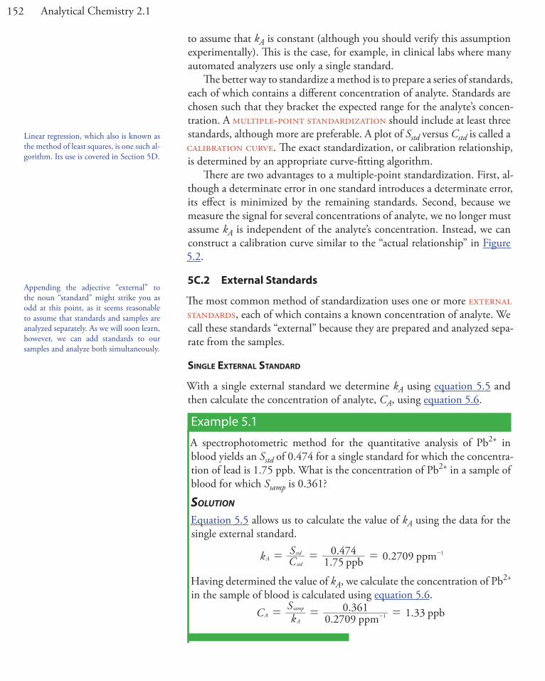
A spectrophotometric method for the quantitative analysis of Pb2+ in blood yields an Sstd of 0.474 for a single standard for which the concentra-tion of lead is 1.75 ppb. What is the concentration of Pb2+ in a sample of blood for which Ssamp is 0.361?
SolutionEquation 5.5 allows us to calculate the value of kA using the data for the single external standard.
.. .k C
S1 75
0 474 0 2709ppb ppmAstd
std 1= = = -
Having determined the value of kA, we calculate the concentration of Pb2+ in the sample of blood is calculated using equation 5.6.
.. .C k
S0 2709
0 361 1 33ppm ppbAA
samp1= = =-
Appending the adjective “external” to the noun “standard” might strike you as odd at this point, as it seems reasonable to assume that standards and samples are analyzed separately. As we will soon learn, however, we can add standards to our samples and analyze both simultaneously.
Linear regression, which also is known as the method of least squares, is one such al-gorithm. Its use is covered in Section 5D.

153Chapter 5 Standardizing Analytical Methods
Multiple external StandardS
Figure 5.3 shows a typical multiple-point external standardization. The volumetric flask on the left contains a reagent blank and the remaining volumetric flasks contain increasing concentrations of Cu2+. Shown be-low the volumetric flasks is the resulting calibration curve. Because this is the most common method of standardization, the resulting relationship is called a normal calibration curve.
When a calibration curve is a straight-line, as it is in Figure 5.3, the slope of the line gives the value of kA. This is the most desirable situation because the method’s sensitivity remains constant throughout the analyte’s concentration range. When the calibration curve is not a straight-line, the method’s sensitivity is a function of the analyte’s concentration. In Figure 5.2, for example, the value of kA is greatest when the analyte’s concentration is small and it decreases continuously for higher concentrations of analyte. The value of kA at any point along the calibration curve in Figure 5.2 is the slope at that point. In either case, a calibration curve allows to relate Ssamp to the analyte’s concentration.
Example 5.2
A second spectrophotometric method for the quantitative analysis of Pb2+ in blood has a normal calibration curve for which
( . ) .S C0 296 0 003ppbstd std1 #= +-
What is the concentration of Pb2+ in a sample of blood if Ssamp is 0.397?
0 0.0020 0.0040 0.0060 0.00800
0.05
0.10
0.15
0.20
Sstd
Cstd (M)
0.25
Figure 5.3 The photo at the top of the figure shows a reagent blank (far left) and a set of five external standards for Cu2+ with concentrations that in-crease from left-to-right. Shown below the external standards is the resulting normal calibration curve. The absorbance of each standard, Sstd, is shown by the filled circles.

154 Analytical Chemistry 2.1
SolutionTo determine the concentration of Pb2+ in the sample of blood, we replace Sstd in the calibration equation with Ssamp and solve for CA.
..
.. . .C S
0 2960 003
0 2960 397 0 003 1 33ppb ppb ppbA
samp1 1=
-= - =- -
It is worth noting that the calibration equation in this problem includes an extra term that does not appear in equation 5.6. Ideally we expect our calibration curve to have a signal of zero when CA is zero. This is the purpose of using a reagent blank to correct the measured signal. The extra term of +0.003 in our calibration equation results from the uncertainty in measuring the signal for the reagent blank and the standards.
An external standardization allows us to analyze a series of samples using a single calibration curve. This is an important advantage when we have many samples to analyze. Not surprisingly, many of the most common quantitative analytical methods use an external standardization.
There is a serious limitation, however, to an external standardization. When we determine the value of kA using equation 5.5, the analyte is pres-ent in the external standard’s matrix, which usually is a much simpler ma-trix than that of our samples. When we use an external standardization we assume the matrix does not affect the value of kA. If this is not true, then we introduce a proportional determinate error into our analysis. This is not the case in Figure 5.4, for instance, where we show calibration curves for an analyte in the sample’s matrix and in the standard’s matrix. In this case, using the calibration curve for the external standards leads to a negative de-terminate error in analyte’s reported concentration. If we expect that matrix effects are important, then we try to match the standard’s matrix to that of the sample, a process known as matrix matching. If we are unsure of the sample’s matrix, then we must show that matrix effects are negligible or use an alternative method of standardization. Both approaches are discussed in the following section.
Practice Exercise 5.1Figure 5.3 shows a normal calibration curve for the quantitative analysis of Cu2+. The equation for the calibration curve is
Sstd = 29.59 M–1 × Cstd + 0.0015
What is the concentration of Cu2+ in a sample whose absorbance, Ssamp, is 0.114? Compare your answer to a one-point standardization where a standard of 3.16 × 10⁻³ M Cu2+ gives a signal of 0.0931.
Click here to review your answer to this exercise.
The one-point standardization in this ex-ercise uses data from the third volumetric flask in Figure 5.3.
The matrix for the external standards in Figure 5.3, for example, is dilute ammo-nia. Because the Cu (NH )3 4
2+ complex absorbs more strongly than Cu2+, adding ammonia increases the signal’s magnitude. If we fail to add the same amount of am-monia to our samples, then we will in-troduce a proportional determinate error into our analysis.

155Chapter 5 Standardizing Analytical Methods
5C.3 Standard Additions
We can avoid the complication of matching the matrix of the standards to the matrix of the sample if we carry out the standardization in the sample. This is known as the method of standard additions.
Single Standard addition
The simplest version of a standard addition is shown in Figure 5.5. First we add a portion of the sample, Vo, to a volumetric flask, dilute it to volume, Vf, and measure its signal, Ssamp. Next, we add a second identical portion of sample to an equivalent volumetric flask along with a spike, Vstd, of an external standard whose concentration is Cstd. After we dilute the spiked sample to the same final volume, we measure its signal, Sspike. The following two equations relate Ssamp and Sspike to the concentration of analyte, CA, in the original sample.
S k C VV
samp A Af
o= 5.7
S k C VV C V
Vspike A A
f
ostd
f
std= +a k 5.8
As long as Vstd is small relative to Vo, the effect of the standard’s matrix on the sample’s matrix is insignificant. Under these conditions the value of kA is the same in equation 5.7 and equation 5.8. Solving both equations for kA and equating gives
C VV
S
C VV C V
VS
Af
o
samp
Af
ostd
f
std
spike=
+ 5.9
which we can solve for the concentration of analyte, CA, in the original sample.
(CA)reported
Ssamp
(CA)actual
standard’smatrix
sample’smatrix
Figure 5.4 Calibration curves for an analyte in the standard’s matrix and in the sample’s matrix. If the matrix affects the value of kA, as is the case here, then we introduce a proportional determinate error into our analysis if we use a normal calibration curve.
The ratios Vo/Vf and Vstd/Vf account for the dilution of the sample and the stan-dard, respectively.

156 Analytical Chemistry 2.1
Example 5.3
A third spectrophotometric method for the quantitative analysis of Pb2+ in blood yields an Ssamp of 0.193 when a 1.00 mL sample of blood is diluted to 5.00 mL. A second 1.00 mL sample of blood is spiked with 1.00 mL of a 1560-ppb Pb2+ external standard and diluted to 5.00 mL, yielding an Sspike of 0.419. What is the concentration of Pb2+ in the original sample of blood?
SolutionWe begin by making appropriate substitutions into equation 5.9 and solv-ing for CA. Note that all volumes must be in the same units; thus, we first covert Vstd from 1.00 mL to 1.00 × 10⁻³ mL.
...
..
..
.C C5 00
1 000 193
5 001 00 1560 5 00
1 00 100 419
mLmL
mLmL ppb mL
mLA A
3#=
+-
..
. ..
C C0 2000 193
0 200 0 31200 419
ppbA A=
+
. . .C C0 0386 0 0602 0 0838ppbA A+ =
. .C0 0452 0 0602 ppbA=
.C 1 33 ppbA=
The concentration of Pb2+ in the original sample of blood is 1.33 ppb.
add Vo of CA add Vstd of Cstd
dilute to Vf
CVVA
o
f
× CVV
CVVA
fstd
std
f
× + ×Concentrationof Analyte
o
Figure 5.5 Illustration showing the method of stan-dard additions. The volumetric flask on the left con-tains a portion of the sample, Vo, and the volumetric flask on the right contains an identical portion of the sample and a spike, Vstd, of a standard solution of the analyte. Both flasks are diluted to the same final vol-ume, Vf. The concentration of analyte in each flask is shown at the bottom of the figure where CA is the ana-lyte’s concentration in the original sample and Cstd is the concentration of analyte in the external standard.

157Chapter 5 Standardizing Analytical Methods
It also is possible to add the standard addition directly to the sample, measuring the signal both before and after the spike (Figure 5.6). In this case the final volume after the standard addition is Vo + Vstd and equation 5.7, equation 5.8, and equation 5.9 become
S k Csamp A A=
S k C V VV C V V
Vspike A A
o std
ostd
o std
std= + + +a k 5.10
CS
C V VV C V V
VS
A
samp
Ao std
ostd
o std
std
spike=
+ + +5.11
Example 5.4
A fourth spectrophotometric method for the quantitative analysis of Pb2+ in blood yields an Ssamp of 0.712 for a 5.00 mL sample of blood. After spik-ing the blood sample with 5.00 mL of a 1560-ppb Pb2+ external standard, an Sspike of 1.546 is measured. What is the concentration of Pb2+ in the original sample of blood?
SolutionTo determine the concentration of Pb2+ in the original sample of blood, we make appropriate substitutions into equation 5.11 and solve for CA.
.
..
..
.C C
0 712
5 0055 00 1560 5 005
5 00 101 546
mLmL ppb mL
mLAA
3#=
+-
.. .
.C C
0 7120 9990 1 558
1 546ppbA A
=+
add Vstd of Cstd
Concentrationof Analyte
Vo Vo
CAC
VV V
CV
V VAo
o s tdstd
std
o s td++
+
Figure 5.6 Illustration showing an alternative form of the method of standard additions. In this case we add the spike of external standard directly to the sample without any further adjust in the volume.
Vo + Vstd = 5.000 mL + 5.00×10⁻³ mL
= 5.005 mL

158 Analytical Chemistry 2.1
. . .C C0 7113 1 109 1 546ppbA A+ =
.C 1 33 ppbA=
The concentration of Pb2+ in the original sample of blood is 1.33 ppb.
Multiple Standard additionS
We can adapt a single-point standard addition into a multiple-point stan-dard addition by preparing a series of samples that contain increasing amounts of the external standard. Figure 5.7 shows two ways to plot a standard addition calibration curve based on equation 5.8. In Figure 5.7a we plot Sspike against the volume of the spikes, Vstd. If kA is constant, then the calibration curve is a straight-line. It is easy to show that the x-intercept is equivalent to –CAVo/Cstd.
Example 5.5
Beginning with equation 5.8 show that the equations in Figure 5.7a for the slope, the y-intercept, and the x-intercept are correct.
SolutionWe begin by rewriting equation 5.8 as
S Vk C V
Vk C Vspike
f
A A o
f
A stdstd#= +
which is in the form of the equation for a straight-line
y = y-intercept + slope × x
where y is Sspike and x is Vstd. The slope of the line, therefore, is kACstd/Vf and the y-intercept is kACAVo/Vf. The x-intercept is the value of x when y is zero, or
Vk C V
Vk V x0 -intercept
f
A A o
f
A std #= +
k C Vk C V V
CC Vx-intercept
A std f
A A o f
std
A o=- =-
Practice Exercise 5.2Beginning with equation 5.8 show that the equations in Figure 5.7b for the slope, the y-intercept, and the x-intercept are correct.
Click here to review your answer to this exercise.
Because we know the volume of the original sample, Vo, and the con-centration of the external standard, Cstd, we can calculate the analyte’s con-centrations from the x-intercept of a multiple-point standard additions.

159Chapter 5 Standardizing Analytical Methods
Example 5.6
A fifth spectrophotometric method for the quantitative analysis of Pb2+ in blood uses a multiple-point standard addition based on equation 5.8. The original blood sample has a volume of 1.00 mL and the standard used for spiking the sample has a concentration of 1560 ppb Pb2+. All samples were diluted to 5.00 mL before measuring the signal. A calibration curve of Sspike versus Vstd has the following equation
.S V0 266 312 mLspike std1 #= + -
What is the concentration of Pb2+ in the original sample of blood?
SolutionTo find the x-intercept we set Sspike equal to zero.
. V0 0 266 312 mL std1 #= + -
-4.00 -2.00 0 2.00 4.00 6.00 8.00 10.00 12.000
0.10
0.20
0.30
0.40
0.50
0.60
Sspike
CstdVstd
Vf×
slope = kA
x-intercept = -CAVo
Vf
0
0.10
0.20
0.30
0.40
0.50
0.60
Sspike
-2.00 0 2.00 4.00 6.00
Cstd
Vstd
slope =kACstd
Vf
x-intercept = -CAVo
y-intercept = kACAVo
Vf
(a)
(b)
(mL)
(mg/L)
y-intercept = kACAVo
Vf
Figure 5.7 Shown at the top of the figure is a set of six standard additions for the determination of Mn2+. The flask on the left is a 25.00 mL sample diluted to 50.00 mL with water. The remaining flasks contain 25.00 mL of sample and, from left-to-right, 1.00, 2.00, 3.00, 4.00, and 5.00 mL spikes of an external standard that is 100.6 mg/L Mn2+. Shown below are two ways to plot the standard additions calibration curve. The absorbance for each standard addition, Sspike, is shown by the filled circles.

160 Analytical Chemistry 2.1
Solving for Vstd, we obtain a value of –8.526 × 10⁻⁴ mL for the x-intercept. Substituting the x-intercept’s value into the equation from Figure 5.7a
. .C
C V C8 526 10 15601 00mL ppb
mLstd
A o A4# #- =- =--
and solving for CA gives the concentration of Pb2+ in the blood sample as 1.33 ppb.
Since we construct a standard additions calibration curve in the sample, we can not use the calibration equation for other samples. Each sample, therefore, requires its own standard additions calibration curve. This is a serious drawback if you have many samples. For example, suppose you need to analyze 10 samples using a five-point calibration curve. For a normal calibration curve you need to analyze only 15 solutions (five standards and ten samples). If you use the method of standard additions, however, you must analyze 50 solutions (each of the ten samples is analyzed five times, once before spiking and after each of four spikes).
uSing a Standard addition to identify Matrix effectS
We can use the method of standard additions to validate an external stan-dardization when matrix matching is not feasible. First, we prepare a nor-mal calibration curve of Sstd versus Cstd and determine the value of kA from its slope. Next, we prepare a standard additions calibration curve using equation 5.8, plotting the data as shown in Figure 5.7b. The slope of this standard additions calibration curve provides an independent determina-tion of kA. If there is no significant difference between the two values of kA, then we can ignore the difference between the sample’s matrix and that of the external standards. When the values of kA are significantly different,
Practice Exercise 5.3Figure 5.7 shows a standard additions calibration curve for the quantita-tive analysis of Mn2+. Each solution contains 25.00 mL of the original sample and either 0, 1.00, 2.00, 3.00, 4.00, or 5.00 mL of a 100.6 mg/L external standard of Mn2+. All standard addition samples were diluted to 50.00 mL with water before reading the absorbance. The equation for the calibration curve in Figure 5.7a is
Sstd = 0.0854 × Vstd + 0.1478
What is the concentration of Mn2+ in this sample? Compare your answer to the data in Figure 5.7b, for which the calibration curve is
Sstd = 0.0425 × Cstd(Vstd/Vf) + 0.1478
Click here to review your answer to this exercise.
161Chapter 5 Standardizing Analytical Methods
then using a normal calibration curve introduces a proportional determi-nate error.
5C.4 Internal Standards
To use an external standardization or the method of standard additions, we must be able to treat identically all samples and standards. When this is not possible, the accuracy and precision of our standardization may suffer. For example, if our analyte is in a volatile solvent, then its concentration will increase if we lose solvent to evaporation. Suppose we have a sample and a standard with identical concentrations of analyte and identical signals. If both experience the same proportional loss of solvent, then their respective concentrations of analyte and signals remain identical. In effect, we can ig-nore evaporation if the samples and the standards experience an equivalent loss of solvent. If an identical standard and sample lose different amounts of solvent, however, then their respective concentrations and signals are no longer equal. In this case a simple external standardization or standard addition is not possible.
We can still complete a standardization if we reference the analyte’s signal to a signal from another species that we add to all samples and stan-dards. The species, which we call an internal standard, must be different than the analyte.
Because the analyte and the internal standard receive the same treat-ment, the ratio of their signals is unaffected by any lack of reproducibility in the procedure. If a solution contains an analyte of concentration CA and an internal standard of concentration CIS, then the signals due to the analyte, SA, and the internal standard, SIS, are
S k CA A A=
S k CIS IS IS=
where kA and kIS are the sensitivities for the analyte and the internal stan-dard, respectively. Taking the ratio of the two signals gives the fundamental equation for an internal standardization.
SS
k Ck C K C
CIS
A
IS IS
A A
IS
A#= = 5.12
Because K is a ratio of the analyte’s sensitivity and the internal standard’s sensitivity, it is not necessary to determine independently values for either kA or kIS.
Single internal Standard
In a single-point internal standardization, we prepare a single standard that contains the analyte and the internal standard, and use it to determine the value of K in equation 5.12.
162 Analytical Chemistry 2.1
K CC
SS
A
IS
std IS
A
std#= a ak k 5.13
Having standardized the method, the analyte’s concentration is given by
C KC
SS
AIS
IS
A
samp#= a k
Example 5.7
A sixth spectrophotometric method for the quantitative analysis of Pb2+ in blood uses Cu2+ as an internal standard. A standard that is 1.75 ppb Pb2+ and 2.25 ppb Cu2+ yields a ratio of (SA/SIS)std of 2.37. A sample of blood spiked with the same concentration of Cu2+ gives a signal ratio, (SA/SIS)samp, of 1.80. What is the concentration of Pb2+ in the sample of blood?
SolutionEquation 5.13 allows us to calculate the value of K using the data for the standard
..
. .K CC
SS
1 752 25
2 37 3 05ppb Pbppb Cu
ppb Pbppb Cu
A
IS
std IS
A
std2
2
2
2
# #= = =+
+
+
+
a ak kThe concentration of Pb2+, therefore, is
.
.. .C K
CSS
3 05
2 251 80 1 33
ppb Pbppb Cuppb Cu
ppb PbAIS
IS
A
samp2
2
22# #= = =
+
+
++a k
Multiple internal StandardS
A single-point internal standardization has the same limitations as a single-point normal calibration. To construct an internal standard calibration curve we prepare a series of standards, each of which contains the same concentration of internal standard and a different concentrations of analyte. Under these conditions a calibration curve of (SA/SIS)std versus CA is linear with a slope of K/CIS.
Example 5.8
A seventh spectrophotometric method for the quantitative analysis of Pb2+
in blood gives a linear internal standards calibration curve for which
( . ) .SS C2 11 0 006ppb
IS
A
stdA
1 #= --a kWhat is the ppb Pb2+ in a sample of blood if (SA/SIS)samp is 2.80?
SolutionTo determine the concentration of Pb2+ in the sample of blood we replace (SA/SIS)std in the calibration equation with (SA/SIS)samp and solve for CA.
Although the usual practice is to prepare the standards so that each contains an identical amount of the internal standard, this is not a requirement.

163Chapter 5 Standardizing Analytical Methods
.
.
.. . .C
SS
2 11
0 006
2 112 80 0 006 1 33ppb ppb PbA
IS
A
samp1 1
2=+
= + =- -+
a k
The concentration of Pb2+ in the sample of blood is 1.33 ppb.
In some circumstances it is not possible to prepare the standards so that each contains the same concentration of internal standard. This is the case, for example, when we prepare samples by mass instead of volume. We can still prepare a calibration curve, however, by plotting (SA/SIS)std versus CA/CIS, giving a linear calibration curve with a slope of K.
5D Linear Regression and Calibration CurvesIn a single-point external standardization we determine the value of kA by measuring the signal for a single standard that contains a known con-centration of analyte. Using this value of kA and our sample’s signal, we then calculate the concentration of analyte in our sample (see Example 5.1). With only a single determination of kA, a quantitative analysis using a single-point external standardization is straightforward.
A multiple-point standardization presents a more difficult problem. Consider the data in Table 5.1 for a multiple-point external standardiza-tion. What is our best estimate of the relationship between Sstd and Cstd? It is tempting to treat this data as five separate single-point standardizations, determining kA for each standard, and reporting the mean value for the five trials. Despite it simplicity, this is not an appropriate way to treat a multiple-point standardization.
So why is it inappropriate to calculate an average value for kA using the data in Table 5.1? In a single-point standardization we assume that the reagent blank (the first row in Table 5.1) corrects for all constant sources of determinate error. If this is not the case, then the value of kA from a single-point standardization has a constant determinate error. Table 5.2 demonstrates how an uncorrected constant error affects our determination
Table 5.1 Data for a Hypothetical Multiple-Point External Standardization
Cstd (arbitrary units) Sstd (arbitrary units) kA = Sstd/ Cstd
0.000 0.00 —0.100 12.36 123.60.200 24.83 124.20.300 35.91 119.70.400 48.79 122.00.500 60.42 122.8
mean value for kA = 122.5
You might wonder if it is possible to in-clude an internal standard in the method of standard additions to correct for both matrix effects and uncontrolled variations between samples; well, the answer is yes as described in the paper “Standard Dilu-tion Analysis,” the full reference for which is Jones, W. B.; Donati, G. L.; Calloway, C. P.; Jones, B. T. Anal. Chem. 2015, 87, 2321-2327.

164 Analytical Chemistry 2.1
of kA. The first three columns show the concentration of analyte in a set of standards, Cstd, the signal without any source of constant error, Sstd, and the actual value of kA for five standards. As we expect, the value of kA is the same for each standard. In the fourth column we add a constant determi-nate error of +0.50 to the signals, (Sstd)e. The last column contains the cor-responding apparent values of kA. Note that we obtain a different value of kA for each standard and that each apparent kA is greater than the true value.
How do we find the best estimate for the relationship between the sig-nal and the concentration of analyte in a multiple-point standardization? Figure 5.8 shows the data in Table 5.1 plotted as a normal calibration curve. Although the data certainly appear to fall along a straight line, the actual calibration curve is not intuitively obvious. The process of determining the best equation for the calibration curve is called linear regression.
5D.1 Linear Regression of Straight Line Calibration Curves
When a calibration curve is a straight-line, we represent it using the follow-ing mathematical equation
y x0 1b b= + 5.14where y is the analyte’s signal, Sstd, and x is the analyte’s concentration, Cstd. The constants b0 and b1 are, respectively, the calibration curve’s expected y-intercept and its expected slope. Because of uncertainty in our measure-ments, the best we can do is to estimate values for b0 and b1, which we represent as b0 and b1. The goal of a linear regression analysis is to de-termine the best estimates for b0 and b1. How we do this depends on the uncertainty in our measurements.
5D.2 Unweighted Linear Regression with Errors in y
The most common method for completing the linear regression for equa-tion 5.14 makes three assumptions:
Table 5.2 Effect of a Constant Determinate Error on the Value of kA From a Single-Point Standardization
Cstd
Sstd (without constant error)
kA = Sstd/ Cstd (actual)
(Sstd)e(with constant error)
kA = (Sstd)e/ Cstd (apparent)
1.00 1.00 1.00 1.50 1.502.00 2.00 1.00 2.50 1.253.00 3.00 1.00 3.50 1.174.00 4.00 1.00 4.50 1.135.00 5.00 1.00 5.50 1.10
mean kA (true) = 1.00 mean kA (apparent) = 1.23

165Chapter 5 Standardizing Analytical Methods
(1) that the difference between our experimental data and the calculated regression line is the result of indeterminate errors that affect y,
(2) that indeterminate errors that affect y are normally distributed, and (3) that the indeterminate errors in y are independent of the value of x.
Because we assume that the indeterminate errors are the same for all stan-dards, each standard contributes equally in our estimate of the slope and the y-intercept. For this reason the result is considered an unweighted linear regression.
The second assumption generally is true because of the central limit the-orem, which we considered in Chapter 4. The validity of the two remaining assumptions is less obvious and you should evaluate them before you accept the results of a linear regression. In particular the first assumption always is suspect because there certainly is some indeterminate error in the measure-ment of x. When we prepare a calibration curve, however, it is not unusual to find that the uncertainty in the signal, Sstd, is significantly larger than the uncertainty in the analyte’s concentration, Cstd. In such circumstances the first assumption is usually reasonable.
How a linear regreSSion workS
To understand the logic of a linear regression consider the example shown in Figure 5.9, which shows three data points and two possible straight-lines that might reasonably explain the data. How do we decide how well these straight-lines fit the data, and how do we determine the best straight-line?
Let’s focus on the solid line in Figure 5.9. The equation for this line is
y b b x0 1= +V 5.15
Figure 5.8 Normal calibration curve data for the hypothetical multiple-point external standardization in Table 5.1.
0.0 0.1 0.2 0.3 0.4 0.5
0
10
20
30
40
50
60
Sstd
Cstd
166 Analytical Chemistry 2.1
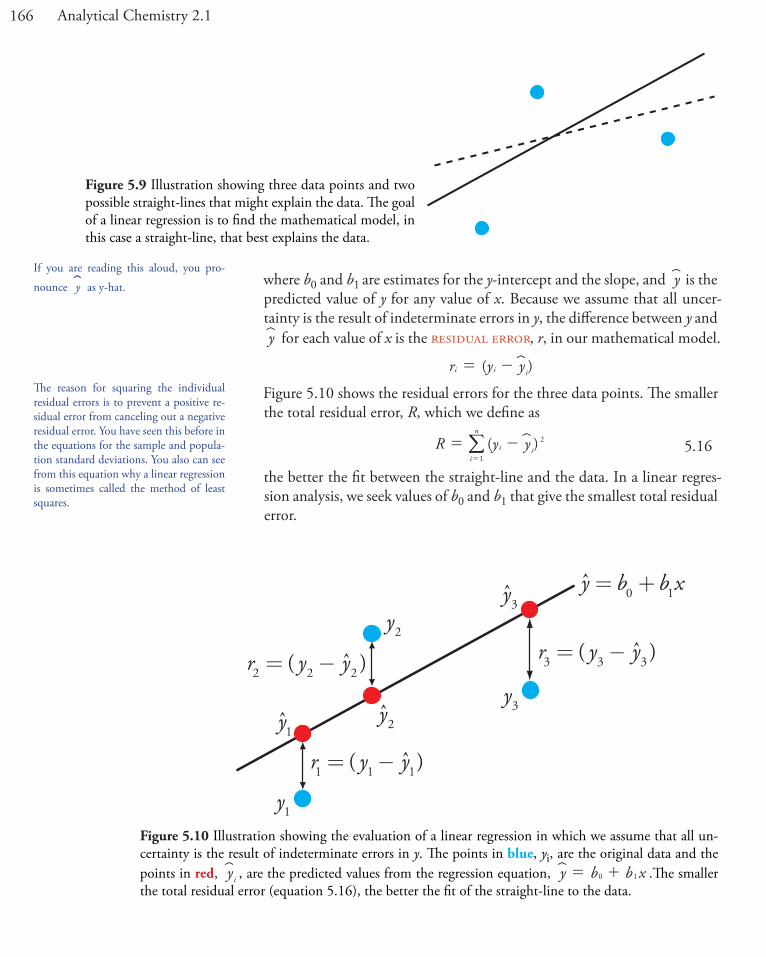
where b0 and b1 are estimates for the y-intercept and the slope, and yV is the predicted value of y for any value of x. Because we assume that all uncer-tainty is the result of indeterminate errors in y, the difference between y and yV for each value of x is the residual error, r, in our mathematical model.
( )r y yi i i= -VFigure 5.10 shows the residual errors for the three data points. The smaller the total residual error, R, which we define as
( )R y yi ii
n2
1= -
=
V/ 5.16
the better the fit between the straight-line and the data. In a linear regres-sion analysis, we seek values of b0 and b1 that give the smallest total residual error.
Figure 5.9 Illustration showing three data points and two possible straight-lines that might explain the data. The goal of a linear regression is to find the mathematical model, in this case a straight-line, that best explains the data.
Figure 5.10 Illustration showing the evaluation of a linear regression in which we assume that all un-certainty is the result of indeterminate errors in y. The points in blue, yi, are the original data and the points in red, yi
V , are the predicted values from the regression equation, y b b x0 1= +V .The smaller the total residual error (equation 5.16), the better the fit of the straight-line to the data.
y1y2
y3
r y y1 1 1= −( ˆ )
r y y2 2 2= −( ˆ ) r y y3 3 3= −( ˆ )
y b b x= +0 1
y1
y2
y3
If you are reading this aloud, you pro-
nounce yT as y-hat.
The reason for squaring the individual residual errors is to prevent a positive re-sidual error from canceling out a negative residual error. You have seen this before in the equations for the sample and popula-tion standard deviations. You also can see from this equation why a linear regression is sometimes called the method of least squares.

167Chapter 5 Standardizing Analytical Methods
finding tHe Slope and y-intercept
Although we will not formally develop the mathematical equations for a linear regression analysis, you can find the derivations in many standard statistical texts.6 The resulting equation for the slope, b1, is
bn x x
n x y x y
ii
n
ii
n
i ii
n
ii
n
ii
n
12
1 1
21 1 1=
-
-
= =
= = =
c m/ // / /
5.17
and the equation for the y-intercept, b0, is
b n
y b xii
n
ii
n
01
11=
-= =
/ / 5.18
Although equation 5.17 and equation 5.18 appear formidable, it is neces-sary only to evaluate the following four summations
x y x y xii
n
ii
n
i ii
n
ii
n
1 1 1
2
1= = = =
/ / / /
Many calculators, spreadsheets, and other statistical software packages are capable of performing a linear regression analysis based on this model. To save time and to avoid tedious calculations, learn how to use one of these tools. For illustrative purposes the necessary calculations are shown in detail in the following example.
Example 5.9
Using the data from Table 5.1, determine the relationship between Sstd and Cstd using an unweighted linear regression.
SolutionWe begin by setting up a table to help us organize the calculation.
xi yi xiyi xi2
0.000 0.00 0.000 0.0000.100 12.36 1.236 0.0100.200 24.83 4.966 0.0400.300 35.91 10.773 0.0900.400 48.79 19.516 0.1600.500 60.42 30.210 0.250
Adding the values in each column gives
xii
n
1=/ = 1.500 yi
i
n
1=/ = 182.31 x yi
i
n
i1=/ = 66.701 xi
i
n2
1=/ = 0.550
Substituting these values into equation 5.17 and equation 5.18, we find that the slope and the y-intercept are
6 See, for example, Draper, N. R.; Smith, H. Applied Regression Analysis, 3rd ed.; Wiley: New York, 1998.
See Section 5F in this chapter for details on completing a linear regression analysis using Excel and R.
Equations 5.17 and 5.18 are written in terms of the general variables x and y. As you work through this example, remem-ber that x corresponds to Cstd, and that y corresponds to Sstd.

168 Analytical Chemistry 2.1
( . ) ( . )( . ) ( . . ) . .b 6 0 550 1 5006 66 701 1 500 182 31 120 706 120 711 2## #
.=-
-=
. ( . . ) . .b 6182 31 120 706 1 500 0 209 0 211
#.=
-=
The relationship between the signal and the analyte, therefore, is
Sstd = 120.71 × Cstd + 0.21
For now we keep two decimal places to match the number of decimal places in the signal. The resulting calibration curve is shown in Figure 5.11.
uncertainty in tHe regreSSion analySiS
As shown in Figure 5.11, because indeterminate errors in the signal, the regression line may not pass through the exact center of each data point. The cumulative deviation of our data from the regression line—that is, the total residual error—is proportional to the uncertainty in the regression. We call this uncertainty the standard deviation about the regression, sr, which is equal to
( )s n
y y
2r
i ii
n2
1= -
-=
V/ 5.19
where yi is the ith experimental value, and yiV is the corresponding value pre-
dicted by the regression line in equation 5.15. Note that the denominator of equation 5.19 indicates that our regression analysis has n–2 degrees of freedom—we lose two degree of freedom because we use two parameters, the slope and the y-intercept, to calculate yi
V .
Figure 5.11 Calibration curve for the data in Table 5.1 and Example 5.9.
0.0 0.1 0.2 0.3 0.4 0.5Cstd
0
10
20
30
40
50
60
Sstd
Did you notice the similarity between the standard deviation about the regression (equation 5.19) and the standard devia-tion for a sample (equation 4.1)?
( )s
n
X X
1
ii
n
1=
-
-=/

169Chapter 5 Standardizing Analytical Methods
A more useful representation of the uncertainty in our regression analy-sis is to consider the effect of indeterminate errors on the slope, b1, and the y-intercept, b0, which we express as standard deviations.
sn x x
nsx x
sb
i ii
n
i
nr
ii
nr
2
1
2
1
2
2
1
2
1 =-
=-
== =
c ^m h// / 5.20
sn x x
s x
n x x
s xb
ii
n
ii
n
r ii
n
ii
n
r ii
n
2
1 1
2
2 2
1
2
1
2 2
10 =
-=
-= =
=
=
=
c ^m h/ //
//
5.21
We use these standard deviations to establish confidence intervals for the expected slope, b1, and the expected y-intercept, b0
b tsb1 1 1!b = 5.22
b tsb0 0 0!b = 5.23where we select t for a significance level of a and for n–2 degrees of free-dom. Note that equation 5.22 and equation 5.23 do not contain a factor of
n 1-^ h because the confidence interval is based on a single regression line.
Example 5.10
Calculate the 95% confidence intervals for the slope and y-intercept from Example 5.9.
SolutionWe begin by calculating the standard deviation about the regression. To do this we must calculate the predicted signals, yi
V , using the slope and y-in-tercept from Example 5.9, and the squares of the residual error, y yi i
2-_ iV .
Using the last standard as an example, we find that the predicted signal is
. ( . . ) .y b b x 0 209 120 706 0 500 60 5626 0 1 6 #= + = + =Vand that the square of the residual error is
( . . ) . .y y 60 42 60 562 0 2016 0 202i i
2 2 .- = - =_ iVThe following table displays the results for all six solutions.
xi yi yiV y yi i
2-_ iV
0.000 0.00 0.209 0.04370.100 12.36 12.280 0.00640.200 24.83 24.350 0.23040.300 35.91 36.421 0.26110.400 48.79 48.491 0.08940.500 60.42 60.562 0.0202
You might contrast equation 5.22 and equation 5.23 with equation 4.12
Xn
ts!n =
for the confidence interval around a sam-ple’s mean value.
As you work through this example, re-member that x corresponds to Cstd, and that y corresponds to Sstd.

170 Analytical Chemistry 2.1
Adding together the data in the last column gives the numerator of equa-tion 5.19 as 0.6512; thus, the standard deviation about the regression is
. .s 6 20 6512 0 4035r = -
=
Next we calculate the standard deviations for the slope and the y-intercept using equation 5.20 and equation 5.21. The values for the summation terms are from in Example 5.9.
( . ) ( . )( . ) .s
n x xns
6 0 550 1 5006 0 4035 0 965b
i ii
n
i
nr
2
1
2
1
2
2
2
1 ##
=-
=-
=
==
c m//
( . ) ( . )( . ) . .s
n x x
s x
6 0 550 1 5000 4035 0 550 0 292b
ii
n
ii
n
r ii
n
2
1 1
2
2 2
12
2
0 ##
=-
=-
=
= =
=
c m/ //
Finally, the 95% confidence intervals (a = 0.05, 4 degrees of freedom) for the slope and y-intercept are
. ( . . ) . .b ts 120 706 2 78 0 965 120 7 2 7b1 1 1! ! # !b = = =
. ( . . ) . .b ts 0 209 2 78 0 292 0 2 0 8b0 0 0! ! # !b = = =
The standard deviation about the regression, sr, suggests that the signal, Sstd, is precise to one decimal place. For this reason we report the slope and the y-intercept to a single decimal place.
MiniMizing uncertainty in calibration curveS
To minimize the uncertainty in a calibration curve’s slope and y-intercept, we evenly space our standards over a wide range of analyte concentrations. A close examination of equation 5.20 and equation 5.21 help us appreci-ate why this is true. The denominators of both equations include the term
x xi2-^ h/ . The larger the value of this term—which we accomplish by
increasing the range of x around its mean value—the smaller the standard deviations in the slope and the y-intercept. Furthermore, to minimize the uncertainty in the y-intercept, it helps to decrease the value of the term
xi/ in equation 5.21, which we accomplish by including standards for lower concentrations of the analyte.
obtaining tHe analyte’S concentration froM a regreSSion equation
Once we have our regression equation, it is easy to determine the concen-tration of analyte in a sample. When we use a normal calibration curve, for example, we measure the signal for our sample, Ssamp, and calculate the analyte’s concentration, CA, using the regression equation.
You can find values for t in Appendix 4.
171Chapter 5 Standardizing Analytical Methods
C bS b
Asamp
1
0=
- 5.24
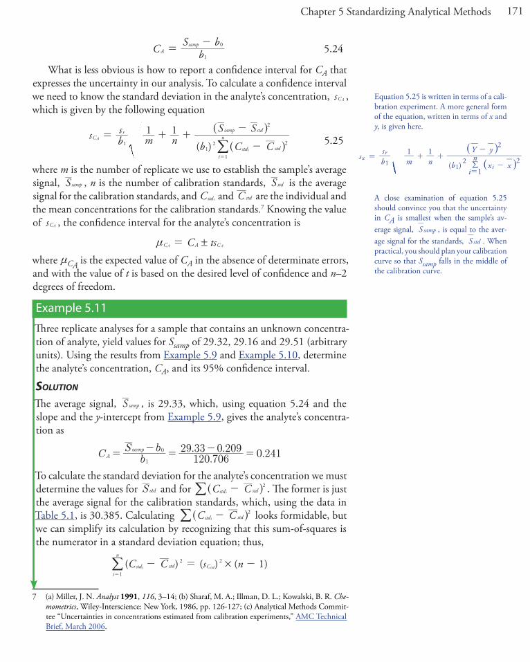
What is less obvious is how to report a confidence interval for CA that expresses the uncertainty in our analysis. To calculate a confidence interval we need to know the standard deviation in the analyte’s concentration, sCA , which is given by the following equation
( )s b
sm n b C C
S S1 1C
r
std stdi
nsamp std
11
2 2
1
2
A
i
= + +-
-
=
^^
hh/ 5.25
where m is the number of replicate we use to establish the sample’s average signal, S samp , n is the number of calibration standards, S std is the average signal for the calibration standards, and Cstdi and C std are the individual and the mean concentrations for the calibration standards.7 Knowing the value of sCA , the confidence interval for the analyte’s concentration is
C tsC A CA A!n =
where nCA is the expected value of CA in the absence of determinate errors, and with the value of t is based on the desired level of confidence and n–2 degrees of freedom.
Example 5.11
Three replicate analyses for a sample that contains an unknown concentra-tion of analyte, yield values for Ssamp of 29.32, 29.16 and 29.51 (arbitrary units). Using the results from Example 5.9 and Example 5.10, determine the analyte’s concentration, CA, and its 95% confidence interval.
SolutionThe average signal, S samp , is 29.33, which, using equation 5.24 and the slope and the y-intercept from Example 5.9, gives the analyte’s concentra-tion as
.. . .C b
S b120 706
29 33 0 209 0 241Asamp
1
0= = - =-
To calculate the standard deviation for the analyte’s concentration we must determine the values for Sstd and for C Cstd std
2i-^ h/ . The former is just
the average signal for the calibration standards, which, using the data in Table 5.1, is 30.385. Calculating C Cstd std
2i-^ h/ looks formidable, but
we can simplify its calculation by recognizing that this sum-of-squares is the numerator in a standard deviation equation; thus,
( ) ( ) ( )C C s n 1std stdi
n
C2
1
2i std #- = -
=
/
7 (a) Miller, J. N. Analyst 1991, 116, 3–14; (b) Sharaf, M. A.; Illman, D. L.; Kowalski, B. R. Che-mometrics, Wiley-Interscience: New York, 1986, pp. 126-127; (c) Analytical Methods Commit-tee “Uncertainties in concentrations estimated from calibration experiments,” AMC Technical Brief, March 2006.
Equation 5.25 is written in terms of a cali-bration experiment. A more general form of the equation, written in terms of x and y, is given here.
( )s b
sm n b x x
Y y1 1x
r
ii
n1 1
2 2
2
1
= + +-
-
=
^^hh/
A close examination of equation 5.25 should convince you that the uncertainty in CA is smallest when the sample’s av-erage signal, S samp , is equal to the aver-age signal for the standards, S std . When practical, you should plan your calibration curve so that Ssamp falls in the middle of the calibration curve.

172 Analytical Chemistry 2.1
where sCstd is the standard deviation for the concentration of analyte in the calibration standards. Using the data in Table 5.1 we find that sCstd is 0.1871 and
( . ) .C C 0 1872 6 1 0 175std stdi
n2 2
1i #- = - =
=
^ ^h h/Substituting known values into equation 5.25 gives
..
( . ) .( . . ) .s 120 706
0 403531
61
120 706 0 17529 33 30 385 0 0024C 2
2
A #= + +
-=
Finally, the 95% confidence interval for 4 degrees of freedom is
. ( . . ) . .C ts 0 241 2 78 0 0024 0 241 0 007C A CA A! ! # !n = = =
Figure 5.12 shows the calibration curve with curves showing the 95% confidence interval for CA.
In a standard addition we determine the analyte’s concentration by extrapolating the calibration curve to the x-intercept. In this case the value of CA is
C x bb-interceptA1
0= = -
and the standard deviation in CA is
( )s b
sn b C C
S1C
r
std stdi
nstd
11
2 2
1
2
A
i
= +-
=
^^h
h/where n is the number of standard additions (including the sample with no added standard), and S std is the average signal for the n standards. Because we determine the analyte’s concentration by extrapolation, rather than by
You can find values for t in Appendix 4.
Figure 5.12 Example of a normal calibration curve with a superimposed confidence interval for the analyte’s con-centration. The points in blue are the original data from Table 5.1. The black line is the normal calibration curve as determined in Example 5.9. The red lines show the 95% confidence interval for CA assuming a single deter-mination of Ssamp.
0
10
20
30
40
50
60
Sstd
0.0 0.1 0.2 0.3 0.4 0.5Cstd

173Chapter 5 Standardizing Analytical Methods
interpolation, sCA for the method of standard additions generally is larger than for a normal calibration curve.
evaluating a linear regreSSion Model
You should never accept the result of a linear regression analysis without evaluating the validity of the model. Perhaps the simplest way to evaluate a regression analysis is to examine the residual errors. As we saw earlier, the residual error for a single calibration standard, ri, is
( )r y yi i i= -
If the regression model is valid, then the residual errors should be distrib-uted randomly about an average residual error of zero, with no apparent trend toward either smaller or larger residual errors (Figure 5.13a). Trends such as those in Figure 5.13b and Figure 5.13c provide evidence that at least one of the model’s assumptions is incorrect. For example, a trend toward larger residual errors at higher concentrations, Figure 5.13b, suggests that the indeterminate errors affecting the signal are not independent of the analyte’s concentration. In Figure 5.13c, the residual errors are not random, which suggests we cannot model the data using a straight-line relationship. Regression methods for the latter two cases are discussed in the following sections.
Practice Exercise 5.4Figure 5.3 shows a normal calibration curve for the quantitative analysis of Cu2+. The data for the calibration curve are shown here.
[Cu2+] (M) Absorbance0 0
1.55×10⁻³ 0.050
3.16×10⁻³ 0.093
4.74×10⁻³ 0.143
6.34×10⁻³ 0.188
7.92×10⁻³ 0.236
Complete a linear regression analysis for this calibration data, reporting the calibration equation and the 95% confidence interval for the slope and the y-intercept. If three replicate samples give an Ssamp of 0.114, what is the concentration of analyte in the sample and its 95% confidence interval?
Click here to review your answer to this exercise.

174 Analytical Chemistry 2.1
5D.3 Weighted Linear Regression with Errors in y
Our treatment of linear regression to this point assumes that indeterminate errors affecting y are independent of the value of x. If this assumption is false, as is the case for the data in Figure 5.13b, then we must include the variance for each value of y into our determination of the y-intercept, bo, and the slope, b1; thus
b n
w y b w xi ii
n
i ii
n
01
11=
-= =
/ / 5.26
bn w x w x
n w x y w x w y
i ii
n
i ii
n
i i ii
n
i ii
n
i ii
n
12
1 1
21 1 1=
-
-
= =
= = =
c m/ // / /
5.27
where wi is a weighting factor that accounts for the variance in yi
ws
n si
yi
ny
2
1
2
i
i=
-
=
-^^hh/ 5.28
and s yi is the standard deviation for yi. In a weighted linear regression, each xy-pair’s contribution to the regression line is inversely proportional to the precision of yi; that is, the more precise the value of y, the greater its contribution to the regression.
Figure 5.13 Plots of the residual error in the signal, Sstd, as a function of the concentration of analyte, Cstd, for an unweighted straight-line regression model. The red line shows a residual error of zero. The distribution of the residual errors in (a) indicates that the unweighted linear regression model is appropriate. The increase in the residual errors in (b) for higher concentrations of analyte, suggests that a weighted straight-line regression is more appropriate. For (c), the curved pattern to the residuals suggests that a straight-line model is inappropriate; linear regression using a quadratic model might produce a better fit.
0.0 0.1 0.2 0.3 0.4 0.5Cstd
0.0 0.1 0.2 0.3 0.4 0.5Cstd
0.0 0.1 0.2 0.3 0.4 0.5Cstd
resi
dual
err
or
resi
dual
err
or
resi
dual
err
or
(a) (b) (c)
Practice Exercise 5.5Using your results from Practice Exercise 5.4, construct a residual plot and explain its significance.
Click here to review your answer to this exercise.

175Chapter 5 Standardizing Analytical Methods
Example 5.12
Shown here are data for an external standardization in which sstd is the standard deviation for three replicate determination of the signal.
Cstd (arbitrary units) Sstd (arbitrary units) sstd0.000 0.00 0.020.100 12.36 0.020.200 24.83 0.070.300 35.91 0.130.400 48.79 0.220.500 60.42 0.33
Determine the calibration curve’s equation using a weighted linear regres-sion.
SolutionWe begin by setting up a table to aid in calculating the weighting factors.
xi yi syi sy2
i
-^ h wi
0.000 0.00 0.02 2500.00 2.83390.100 12.36 0.02 2500.00 2.83390.200 24.83 0.07 204.08 0.23130.300 35.91 0.13 59.17 0.06710.400 48.79 0.22 20.66 0.02340.500 60.42 0.33 9.18 0.0104
Adding together the values in the forth column gives
s yi
n2
1i-
=
^ h/which we use to calculate the individual weights in the last column. After we calculate the individual weights, we use a second table to aid in calculat-ing the four summation terms in equation 5.26 and equation 5.27.
xi yi wi wi xi wi yi wi xi2 wi xi yi
0.000 0.00 2.8339 0.0000 0.0000 0.0000 0.00000.100 12.36 2.8339 0.2834 35.0270 0.0283 3.50270.200 24.83 0.2313 0.0463 5.7432 0.0093 1.14860.300 35.91 0.0671 0.0201 2.4096 0.0060 0.72290.400 48.79 0.0234 0.0094 1.1417 0.0037 0.45670.500 60.42 0.0104 0.0052 0.6284 0.0026 0.3142
Adding the values in the last four columns gives
This is the same data used in Example 5.9 with additional information about the standard deviations in the signal.
As you work through this example, re-member that x corresponds to Cstd, and that y corresponds to Sstd.
As a check on your calculations, the sum of the individual weights must equal the number of calibration standards, n. The sum of the entries in the last column is 6.0000, so all is well.

176 Analytical Chemistry 2.1
. .w x w y0 3644 44 9499i ii
n
i ii
n
1 1= =
= =
/ /
. .w x w x y0 0499 6 1451i ii
n
i ii
n
i2
1 1= =
= =
/ /Substituting these values into the equation 5.26 and equation 5.27 gives the estimated slope and estimated y-intercept as
( . ) ( . )( . ) ( . . ) .b 6 0 0499 0 36446 6 1451 0 3644 44 9499 122 9851 2## #
=-
-=
. ( . . ) .b 644 9499 122 985 0 3644 0 02240
#=
-=
The calibration equation is
. .S C122 98 0 02std std#= +
Figure 5.14 shows the calibration curve for the weighted regression and the calibration curve for the unweighted regression in Example 5.9. Although the two calibration curves are very similar, there are slight differences in the slope and in the y-intercept. Most notably, the y-intercept for the weighted linear regression is closer to the expected value of zero. Because the stan-dard deviation for the signal, Sstd, is smaller for smaller concentrations of analyte, Cstd, a weighted linear regression gives more emphasis to these standards, allowing for a better estimate of the y-intercept.
Figure 5.14 A comparison of the unweighted and the weighted normal calibra-tion curves. See Example 5.9 for details of the unweighted linear regression and Example 5.12 for details of the weighted linear regression.
0.0 0.1 0.2 0.3 0.4 0.5Cstd
0
10
20
30
40
50
60
Sstd
unweighted linear regressionweighted linear regression

177Chapter 5 Standardizing Analytical Methods
Equations for calculating confidence intervals for the slope, the y-in-tercept, and the concentration of analyte when using a weighted linear regression are not as easy to define as for an unweighted linear regression.8 The confidence interval for the analyte’s concentration, however, is at its optimum value when the analyte’s signal is near the weighted centroid, yc , of the calibration curve.
y n w x1c i i
i
n
1=
=
/
5D.4 Weighted Linear Regression with Errors in Both x and y
If we remove our assumption that indeterminate errors affecting a calibra-tion curve are present only in the signal (y), then we also must factor into the regression model the indeterminate errors that affect the analyte’s con-centration in the calibration standards (x). The solution for the resulting regression line is computationally more involved than that for either the unweighted or weighted regression lines.9 Although we will not consider the details in this textbook, you should be aware that neglecting the pres-ence of indeterminate errors in x can bias the results of a linear regression.
5D.5 Curvilinear and Multivariate Regression
A straight-line regression model, despite its apparent complexity, is the simplest functional relationship between two variables. What do we do if our calibration curve is curvilinear—that is, if it is a curved-line instead of a straight-line? One approach is to try transforming the data into a straight-line. Logarithms, exponentials, reciprocals, square roots, and trigonometric functions have been used in this way. A plot of log(y) versus x is a typical example. Such transformations are not without complications, of which the most obvious is that data with a uniform variance in y will not maintain that uniform variance after it is transformed.
Another approach to developing a linear regression model is to fit a polynomial equation to the data, such as y = a + bx + cx2. You can use linear regression to calculate the parameters a, b, and c, although the equa-tions are different than those for the linear regression of a straight-line.10 If you cannot fit your data using a single polynomial equation, it may be possible to fit separate polynomial equations to short segments of the cali-bration curve. The result is a single continuous calibration curve known as a spline function.
8 Bonate, P. J. Anal. Chem. 1993, 65, 1367–1372.9 See, for example, Analytical Methods Committee, “Fitting a linear functional relationship to
data with error on both variable,” AMC Technical Brief, March, 2002), as well as this chapter’s Additional Resources.
10 For details about curvilinear regression, see (a) Sharaf, M. A.; Illman, D. L.; Kowalski, B. R. Chemometrics, Wiley-Interscience: New York, 1986; (b) Deming, S. N.; Morgan, S. L. Experi-mental Design: A Chemometric Approach, Elsevier: Amsterdam, 1987.
See Figure 5.2 for an example of a calibra-tion curve that deviates from a straight-line for higher concentrations of analyte.
It is worth noting that the term “linear” does not mean a straight-line. A linear function may contain more than one ad-ditive term, but each such term has one and only one adjustable multiplicative parameter. The function
y = ax + bx2
is an example of a linear function because the terms x and x2 each include a single multiplicative parameter, a and b, respec-tively. The function
y = xb
is nonlinear because b is not a multiplica-tive parameter; it is, instead, a power. This is why you can use linear regression to fit a polynomial equation to your data.
Sometimes it is possible to transform a nonlinear function into a linear function. For example, taking the log of both sides of the nonlinear function above gives a linear function.
log(y) = blog(x)

178 Analytical Chemistry 2.1
The regression models in this chapter apply only to functions that con-tain a single independent variable, such as a signal that depends upon the analyte’s concentration. In the presence of an interferent, however, the signal may depend on the concentrations of both the analyte and the interferent
S k C k C SA A I I reag= + +
where kI is the interferent’s sensitivity and CI is the interferent’s concentra-tion. Multivariate calibration curves are prepared using standards that con-tain known amounts of both the analyte and the interferent, and modeled using multivariate regression.11
5E Compensating for the Reagent Blank (Sreag)Thus far in our discussion of strategies for standardizing analytical methods, we have assumed that a suitable reagent blank is available to correct for sig-nals arising from sources other than the analyte. We did not, however ask an important question: “What constitutes an appropriate reagent blank?” Surprisingly, the answer is not immediately obvious.
In one study, approximately 200 analytical chemists were asked to evaluate a data set consisting of a normal calibration curve, a separate ana-lyte-free blank, and three samples with different sizes, but drawn from the same source.12 The first two columns in Table 5.3 shows a series of external standards and their corresponding signals. The normal calibration curve for the data is
Sstd = 0.0750 × Wstd + 0.1250
where the y-intercept of 0.1250 is the calibration blank. A separate reagent blank gives the signal for an analyte-free sample.
11 Beebe, K. R.; Kowalski, B. R. Anal. Chem. 1987, 59, 1007A–1017A.12 Cardone, M. J. Anal. Chem. 1986, 58, 433–438.
Check out this chapter’s Additional Re-sources at the end of the textbook for more information about linear regression with errors in both variables, curvilinear regression, and multivariate regression.
Table 5.3 Data Used to Study the Blank in an Analytical MethodWstd Sstd Sample Number Wsamp Ssamp
1.6667 0.2500 1 62.4746 0.80005.0000 0.5000 2 82.7915 1.00008.3333 0.7500 3 103.1085 1.2000
11.6667 0.841318.1600 1.4870 reagent blank 0.100019.9333 1.6200
Calibration equation: Sstd = 0.0750 × Wstd + 0.1250Wstd: weight of analyte used to prepare the external standard; diluted to volume, V.Wsamp: weight of sample used to prepare sample; diluted to volume, V.

179Chapter 5 Standardizing Analytical Methods
In working up this data, the analytical chemists used at least four dif-ferent approaches to correct the signals: (a) ignoring both the calibration blank, CB, and the reagent blank, RB, which clearly is incorrect; (b) using the calibration blank only; (c) using the reagent blank only; and (d) using both the calibration blank and the reagent blank. The first four rows of Table 5.4 shows the equations for calculating the analyte’s concentration using each approach, along with the reported concentrations for the analyte in each sample.
That all four methods give a different result for the analyte’s concentra-tion underscores the importance of choosing a proper blank, but does not tell us which blank is correct. Because all four methods fail to predict the same concentration of analyte for each sample, none of these blank correc-tions properly accounts for an underlying constant source of determinate error.
To correct for a constant method error, a blank must account for sig-nals from any reagents and solvents used in the analysis and any bias that results from interactions between the analyte and the sample’s matrix. Both the calibration blank and the reagent blank compensate for signals from reagents and solvents. Any difference in their values is due to indeterminate errors in preparing and analyzing the standards.
Unfortunately, neither a calibration blank nor a reagent blank can cor-rect for a bias that results from an interaction between the analyte and the sample’s matrix. To be effective, the blank must include both the sample’s matrix and the analyte and, consequently, it must be determined using the sample itself. One approach is to measure the signal for samples of differ-
Table 5.4 Equations and Resulting Concentrations of Analyte for Different Approaches to Correcting for the Blank
Concentration of Analyte in...Approach for Correcting The Signal Equation Sample 1 Sample 2 Sample 3
ignore calibration and reagent blank C WW
k WS
Asamp
A
A samp
samp= = 0.1707 0.1610 0.1552
use calibration blank only C WW
k WS CB
Asamp
A
A samp
samp= =
-0.1441 0.1409 0.1390
use reagent blank only C WW
k WS RB
Asamp
A
A samp
samp= =
-0.1494 0.1449 0.1422
use both calibration and reagent blank C WW
k WS CB RB
Asamp
A
A samp
samp= =
- -0.1227 0.1248 0.1261
use total Youden blank C WW
k WS TYB
Asamp
A
A samp
samp= =
-0.1313 0.1313 0.1313
CA = concentration of analyte; WA = weight of analyte; Wsamp = weight of sample; kA = slope of calibration curve (0.075; see Table 5.3); CB = calibration blank (0.125; see Table 5.3); RB = reagent blank (0.100; see Table 5.3); TYB = total Youden blank (0.185; see text)
Because we are considering a matrix effect of sorts, you might think that the method of standard additions is one way to over-come this problem. Although the method of standard additions can compensate for proportional determinate errors, it cannot correct for a constant determinate error; see Ellison, S. L. R.; Thompson, M. T. “Standard additions: myth and reality,” Analyst, 2008, 133, 992–997.

180 Analytical Chemistry 2.1
ent size, and to determine the regression line for a plot of Ssamp versus the amount of sample. The resulting y-intercept gives the signal in the absence of sample, and is known as the total Youden blank.13 This is the true blank correction. The regression line for the three samples in Table 5.3 is
Ssamp = 0.009844 × Wsamp + 0.185
giving a true blank correction of 0.185. As shown by the last row of Table 5.4, using this value to correct Ssamp gives identical values for the concentra-tion of analyte in all three samples.
The use of the total Youden blank is not common in analytical work, with most chemists relying on a calibration blank when using a calibra-tion curve and a reagent blank when using a single-point standardization. As long we can ignore any constant bias due to interactions between the analyte and the sample’s matrix, which is often the case, the accuracy of an analytical method will not suffer. It is a good idea, however, to check for constant sources of error before relying on either a calibration blank or a reagent blank.
5F Using Excel and R for a Regression AnalysisAlthough the calculations in this chapter are relatively straightforward—consisting, as they do, mostly of summations—it is tedious to work through problems using nothing more than a calculator. Both Excel and R include functions for completing a linear regression analysis and for visually evalu-ating the resulting model.
5F.1 Excel
Let’s use Excel to fit the following straight-line model to the data in Ex-ample 5.9.
y x0 1b b= +
Enter the data into a spreadsheet, as shown in Figure 5.15. Depending upon your needs, there are many ways that you can use Excel to complete a linear regression analysis. We will consider three approaches here.
uSe excel’S built-in functionS
If all you need are values for the slope, b1, and the y-intercept, b0, you can use the following functions:
= intercept(known_y’s, known_x’s)
= slope(known_y’s, known_x’s)
13 Cardone, M. J. Anal. Chem. 1986, 58, 438–445.
Figure 5.15 Portion of a spread-sheet containing data from Exam-ple 5.9 (Cstd = Cstd; Sstd = Sstd).
A B1 Cstd Sstd2 0.000 0.003 0.100 12.364 0.200 24.835 0.300 35.916 0.400 48.797 0.500 60.42

181Chapter 5 Standardizing Analytical Methods
where known_y’s is the range of cells that contain the signals (y), and known_x’s is the range of cells that contain the concentrations (x). For ex-ample, if you click on an empty cell and enter
= slope(B2:B7, A2:A7)
Excel returns exact calculation for the slope (120.705 714 3).
uSe excel’S data analySiS toolS
To obtain the slope and the y-intercept, along with additional statistical details, you can use the data analysis tools in the Data Analysis ToolPak. The ToolPak is not a standard part of Excel’s instillation. To see if you have access to the Analysis ToolPak on your computer, select Tools from the menu bar and look for the Data Analysis... option. If you do not see Data Analysis..., select Add-ins... from the Tools menu. Check the box for the Analysis ToolPak and click on OK to install them.
Select Data Analysis... from the Tools menu, which opens the Data Analysis window. Scroll through the window, select Regression from the available options, and press OK. Place the cursor in the box for Input Y range and then click and drag over cells B1:B7. Place the cursor in the box for Input X range and click and drag over cells A1:A7. Because cells A1 and B1 contain labels, check the box for Labels. Select the radio button for Output range and click on any empty cell; this is where Excel will place the results. Clicking OK generates the information shown in Figure 5.16.
There are three parts to Excel’s summary of a regression analysis. At the top of Figure 5.16 is a table of Regression Statistics. The standard error is the standard deviation about the regression, sr. Also of interest is the value for Multiple R, which is the model’s correlation coefficient, r, a term with which you may already be familiar. The correlation coefficient is a measure of the extent to which the regression model explains the variation in y. Values of r
Excel’s Data Analysis Toolpak is available for Windows. Older versions of Excel for Mac included the toolpak; however, beginning with Excel for Mac 2011, the toolpak no longer is available.
Once you install the Analysis ToolPak, it will continue to load each time you launch Excel.
Including labels is a good idea. Excel’s summary output uses the x-axis label to identify the slope.
Figure 5.16 Output from Excel’s Regression command in the Analysis ToolPak. See the text for a discussion of how to interpret the information in these tables.
SUMMARY OUTPUT
Regression StatisticsMultiple R 0.99987244R Square 0.9997449Adjusted R Square 0.99968113Standard Error 0.40329713Observations 6
ANOVAdf SS MS F Significance F
Regression 1 2549.727156 2549.72716 15676.296 2.4405E-08Residual 4 0.650594286 0.16264857Total 5 2550.37775
Coefficients Standard Error t Stat P-value Lower 95% Upper 95% Lower 95.0% Upper 95.0%Intercept 0.20857143 0.29188503 0.71456706 0.51436267 -0.60183133 1.01897419 -0.60183133 1.01897419Cstd 120.705714 0.964064525 125.205016 2.4405E-08 118.029042 123.382387 118.029042 123.382387
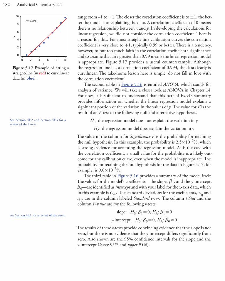
182 Analytical Chemistry 2.1
range from –1 to +1. The closer the correlation coefficient is to ±1, the bet-ter the model is at explaining the data. A correlation coefficient of 0 means there is no relationship between x and y. In developing the calculations for linear regression, we did not consider the correlation coefficient. There is a reason for this. For most straight-line calibration curves the correlation coefficient is very close to +1, typically 0.99 or better. There is a tendency, however, to put too much faith in the correlation coefficient’s significance, and to assume that an r greater than 0.99 means the linear regression model is appropriate. Figure 5.17 provides a useful counterexample. Although the regression line has a correlation coefficient of 0.993, the data clearly is curvilinear. The take-home lesson here is simple: do not fall in love with the correlation coefficient!
The second table in Figure 5.16 is entitled ANOVA, which stands for analysis of variance. We will take a closer look at ANOVA in Chapter 14. For now, it is sufficient to understand that this part of Excel’s summary provides information on whether the linear regression model explains a significant portion of the variation in the values of y. The value for F is the result of an F-test of the following null and alternative hypotheses.
H0: the regression model does not explain the variation in y
HA: the regression model does explain the variation in y
The value in the column for Significance F is the probability for retaining the null hypothesis. In this example, the probability is 2.5×10⁻⁶%, which is strong evidence for accepting the regression model. As is the case with the correlation coefficient, a small value for the probability is a likely out-come for any calibration curve, even when the model is inappropriate. The probability for retaining the null hypothesis for the data in Figure 5.17, for example, is 9.0×10⁻⁷%.
The third table in Figure 5.16 provides a summary of the model itself. The values for the model’s coefficients—the slope, b1, and the y-intercept, b0—are identified as intercept and with your label for the x-axis data, which in this example is Cstd. The standard deviations for the coefficients, sb0 and sb1, are in the column labeled Standard error. The column t Stat and the column P-value are for the following t-tests.
slope H0: b1 = 0, HA: b1 ≠ 0
y-intercept H0: b0 = 0, HA: b0 ≠ 0
The results of these t-tests provide convincing evidence that the slope is not zero, but there is no evidence that the y-intercept differs significantly from zero. Also shown are the 95% confidence intervals for the slope and the y-intercept (lower 95% and upper 95%).
Figure 5.17 Example of fitting a straight-line (in red) to curvilinear data (in blue).
0 2 4 6 8 10
0
2
4
6
8
10
x
y
r = 0.993
See Section 4F.2 and Section 4F.3 for a review of the F-test.
See Section 4F.1 for a review of the t-test.

183Chapter 5 Standardizing Analytical Methods
prograM tHe forMulaS yourSelf
A third approach to completing a regression analysis is to program a spread-sheet using Excel’s built-in formula for a summation
=sum(first cell:last cell)and its ability to parse mathematical equations. The resulting spreadsheet is shown in Figure 5.18.
uSing excel to viSualize tHe regreSSion Model
You can use Excel to examine your data and the regression line. Begin by plotting the data. Organize your data in two columns, placing the x values in the left-most column. Click and drag over the data and select Charts from the ribbon. Select Scatter, choosing the option without lines that connect the points. To add a regression line to the chart, click on the chart’s data and select Chart: Add Trendline... from the main men. Pick the straight-line model and click OK to add the line to your chart. By default, Excel displays the regression line from your first point to your last point. Figure 5.19 shows the result for the data in Figure 5.15.
Excel also will create a plot of the regression model’s residual errors. To create the plot, build the regression model using the Analysis ToolPak, as described earlier. Clicking on the option for Residual plots creates the plot shown in Figure 5.20.
liMitationS to uSing excel for a regreSSion analySiS
Excel’s biggest limitation for a regression analysis is that it does not provide a function to calculate the uncertainty when predicting values of x. In terms of this chapter, Excel can not calculate the uncertainty for the analyte’s
Figure 5.18 Spreadsheet showing the formulas for calculating the slope and the y-intercept for the data in Example 5.9. The shaded cells contain formulas that you must enter. Enter the formulas in cells C3 to C7, and cells D3 to D7. Next, enter the formulas for cells A9 to D9. Finally, enter the formulas in cells F2 and F3. When you enter a formula, Excel replaces it with the resulting calculation. The values in these cells should agree with the results in Example 5.9. You can simplify the entering of formulas by copying and pasting. For example, enter the formula in cell C2. Select Edit: Copy, click and drag your cursor over cells C3 to C7, and select Edit: Paste. Excel automatically updates the cell referencing.
A B C D E F
1 x y xy x^2 n = 62 0.000 0.00 =A2*B2 =A2^2 slope = =(F1*C8 - A8*B8)/(F1*D8-A8^2)3 0.100 12.36 =A3*B3 =A3^2 y-int = =(B8-F2*A8)/F14 0.200 24.83 =A4*B4 =A4^25 0.300 35.91 =A5*B5 =A5^26 0.400 48.79 =A6*B6 =A6^27 0.500 60.42 =A7*B7 =A7^28
9 =sum(A2:A7) =sum(B2:B7) =sum(C2:C7) =sum(D2:D7) <--sums

184 Analytical Chemistry 2.1
concentration, CA, given the signal for a sample, Ssamp. Another limitation is that Excel does not have a built-in function for a weighted linear regres-sion. You can, however, program a spreadsheet to handle these calculations.
5F.2 R
Let’s use R to fit the following straight-line model to the data in Example 5.9.
y x0 1b b= +
entering data and creating tHe regreSSion Model
To begin, create objects that contain the concentration of the standards and their corresponding signals.
> conc = c(0, 0.1, 0.2, 0.3, 0.4, 0.5)> signal = c(0, 12.36, 24.83, 35.91, 48.79, 60.42)
Figure 5.19 Example of an Excel scatterplot showing the data and a regression line.
0
10
20
30
40
50
60
70
0 0.1 0.2 0.3 0.4 0.5 0.6
x-axis
y-axisy-a
xis
-0.6
-0.4
-0.2
0
0.2
0.4
0.6
0 0.1 0.2 0.3 0.4 0.5 0.6
Cstd
ResidualsResi
du
als
Figure 5.20 Example of Excel’s plot of a re-gression model’s residual errors.
Practice Exercise 5.6Use Excel to complete the regression analysis in Practice Exercise 5.4.
Click here to review your an-swer to this exercise.

185Chapter 5 Standardizing Analytical Methods
The command for a straight-line linear regression model is
lm(y ~ x)
where y and x are the objects the objects our data. To access the results of the regression analysis, we assign them to an object using the following command
> model = lm(signal ~ conc)where model is the name we assign to the object.
evaluating tHe linear regreSSion Model
To evaluate the results of a linear regression we need to examine the data and the regression line, and to review a statistical summary of the model. To examine our data and the regression line, we use the plot command, which takes the following general form
plot(x, y, optional arguments to control style)
where x and y are the objects that contain our data, and the abline com-mand
abline(object, optional arguments to control style)
where object is the object that contains the results of the linear regression. Entering the commands
> plot(conc, signal, pch = 19, col = “blue”, cex = 2)> abline(model, col = “red”)
creates the plot shown in Figure 5.21. To review a statistical summary of the regression model, we use the
summary command.> summary(model)
As you might guess, lm is short for linear model.
You can choose any name for the object that contains the results of the regression analysis.
The name abline comes from the follow-ing common form for writing the equa-tion of a straight-line.
y = a + bx
where a is the y-intercept and b is the slope.
Figure 5.21 Example of a regression plot in R showing the data (in blue)and the regression line (in red). You can customize your plot by adjusting the plot command’s optional arguments. For example, the argument pch controls the symbol used for plotting points, the argument col allows you to select a color for the points or the line, and the argument cex sets the size for the points. You can use the command
help(plot) to learn more about the options for plotting data in R.
0.0 0.1 0.2 0.3 0.4 0.5
010
2030
4050
60
conc
sign
al
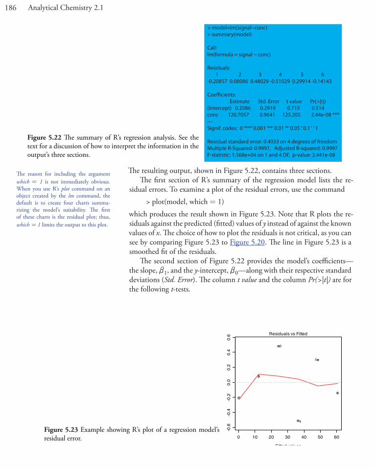
186 Analytical Chemistry 2.1
The resulting output, shown in Figure 5.22, contains three sections. The first section of R’s summary of the regression model lists the re-
sidual errors. To examine a plot of the residual errors, use the command> plot(model, which = 1)
which produces the result shown in Figure 5.23. Note that R plots the re-siduals against the predicted (fitted) values of y instead of against the known values of x. The choice of how to plot the residuals is not critical, as you can see by comparing Figure 5.23 to Figure 5.20. The line in Figure 5.23 is a smoothed fit of the residuals.
The second section of Figure 5.22 provides the model’s coefficients—the slope, b1, and the y-intercept, b0—along with their respective standard deviations (Std. Error). The column t value and the column Pr(>|t|) are for the following t-tests.
The reason for including the argument which = 1 is not immediately obvious. When you use R’s plot command on an object created by the lm command, the default is to create four charts summa-rizing the model’s suitability. The first of these charts is the residual plot; thus, which = 1 limits the output to this plot.
Figure 5.22 The summary of R’s regression analysis. See the text for a discussion of how to interpret the information in the output’s three sections.
> model=lm(signal~conc)> summary(model)
Call:lm(formula = signal ~ conc)
Residuals: 1 2 3 4 5 6 -0.20857 0.08086 0.48029 -0.51029 0.29914 -0.14143
Coe�cients: Estimate Std. Error t value Pr(>|t|) (Intercept) 0.2086 0.2919 0.715 0.514 conc 120.7057 0.9641 125.205 2.44e-08 ***---Signif. codes: 0 ‘***’ 0.001 ‘**’ 0.01 ‘*’ 0.05 ‘.’ 0.1 ‘ ’ 1
Residual standard error: 0.4033 on 4 degrees of freedomMultiple R-Squared: 0.9997, Adjusted R-squared: 0.9997 F-statistic: 1.568e+04 on 1 and 4 DF, p-value: 2.441e-08
Figure 5.23 Example showing R’s plot of a regression model’s residual error. 0 10 20 30 40 50 60
-0.6
-0.4
-0.2
0.0
0.2
0.4
0.6
Fitted values
Res
idua
ls
lm(signal ~ conc)
Residuals vs Fitted
4
3
5

187Chapter 5 Standardizing Analytical Methods
slope H0: b1 = 0, HA: b1 ≠ 0
y-intercept H0: b0 = 0, HA: b0 ≠ 0
The results of these t-tests provide convincing evidence that the slope is not zero, but no evidence that the y-intercept differs significantly from zero.
The last section of the regression summary provides the standard devia-tion about the regression (residual standard error), the square of the cor-relation coefficient (multiple R-squared), and the result of an F-test on the model’s ability to explain the variation in the y values. For a discussion of the correlation coefficient and the F-test of a regression model, as well as their limitations, refer to the section on using Excel’s data analysis tools.
predicting tHe uncertainty in CA given SSAmp
Unlike Excel, R includes a command for predicting the uncertainty in an analyte’s concentration, CA, given the signal for a sample, Ssamp. This com-mand is not part of R’s standard installation. To use the command you need to install the “chemCal” package by entering the following command (note: you will need an internet connection to download the package).
> install.packages(“chemCal”)After installing the package, you need to load the functions into R using the following command. (note: you will need to do this step each time you begin a new R session as the package does not automatically load when you start R).
> library(“chemCal”)The command for predicting the uncertainty in CA is inverse.predict,
which takes the following form for an unweighted linear regression
inverse.predict(object, newdata, alpha = value)
where object is the object that contains the regression model’s results, new-data is an object that contains values for Ssamp, and value is the numerical value for the significance level. Let’s use this command to complete Ex-ample 5.11. First, we create an object that contains the values of Ssamp
> sample = c(29.32, 29.16, 29.51)and then we complete the computation using the following command
> inverse.predict(model, sample, alpha = 0.05) producing the result shown in Figure 5.24. The analyte’s concentration, CA, is given by the value $Prediction, and its standard deviation, sCA, is shown as $`Standard Error`. The value for $Confidence is the confidence interval, ±tsCA, for the analyte’s concentration, and $`Confidence Limits` provides the lower limit and upper limit for the confidence interval for CA.
See Section 4F.1 for a review of the t-test.
See Section 4F.2 and Section 4F.3 for a review of the F-test.
You need to install a package once, but you need to load the package each time you plan to use it. There are ways to con-figure R so that it automatically loads certain packages; see An Introduction to R for more information (click here to view a PDF version of this document).
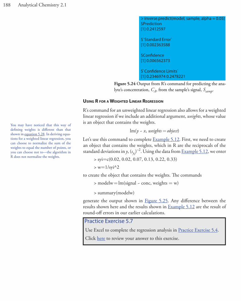
188 Analytical Chemistry 2.1
uSing r for a weigHted linear regreSSion
R’s command for an unweighted linear regression also allows for a weighted linear regression if we include an additional argument, weights, whose value is an object that contains the weights.
lm(y ~ x, weights = object)
Let’s use this command to complete Example 5.12. First, we need to create an object that contains the weights, which in R are the reciprocals of the standard deviations in y, (syi)
–2. Using the data from Example 5.12, we enter> syi=c(0.02, 0.02, 0.07, 0.13, 0.22, 0.33)> w=1/syi^2
to create the object that contains the weights. The commands> modelw = lm(signal ~ conc, weights = w)
> summary(modelw)generate the output shown in Figure 5.25. Any difference between the results shown here and the results shown in Example 5.12 are the result of round-off errors in our earlier calculations.
Figure 5.24 Output from R’s command for predicting the ana-lyte’s concentration, CA, from the sample’s signal, Ssamp.
> inverse.predict(model, sample, alpha = 0.05)$Prediction[1] 0.2412597
$`Standard Error`[1] 0.002363588
$Con�dence[1] 0.006562373
$`Con�dence Limits`[1] 0.2346974 0.2478221
You may have noticed that this way of defining weights is different than that shown in equation 5.28. In deriving equa-tions for a weighted linear regression, you can choose to normalize the sum of the weights to equal the number of points, or you can choose not to—the algorithm in R does not normalize the weights.
Practice Exercise 5.7Use Excel to complete the regression analysis in Practice Exercise 5.4.
Click here to review your answer to this exercise.
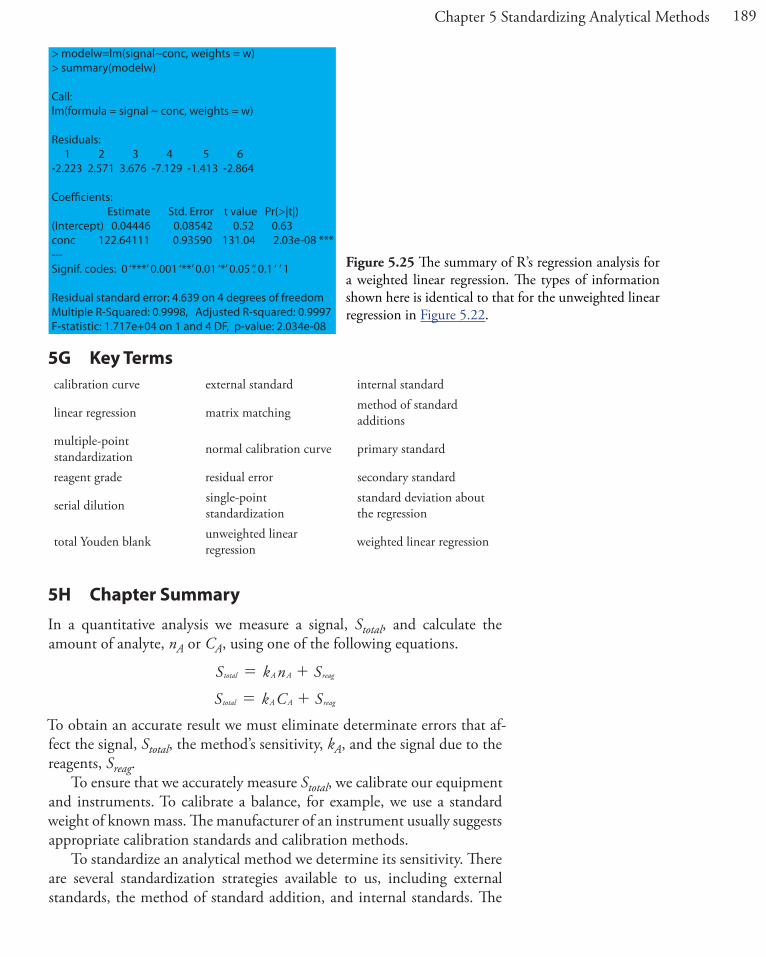
189Chapter 5 Standardizing Analytical Methods
5G Key Termscalibration curve external standard internal standard
linear regression matrix matching method of standard additions
multiple-point standardization normal calibration curve primary standard
reagent grade residual error secondary standard
serial dilution single-point standardization
standard deviation about the regression
total Youden blank unweighted linear regression weighted linear regression
5H Chapter SummaryIn a quantitative analysis we measure a signal, Stotal, and calculate the amount of analyte, nA or CA, using one of the following equations.
S k n Stotal A A reag= +
S k C Stotal A A reag= +
To obtain an accurate result we must eliminate determinate errors that af-fect the signal, Stotal, the method’s sensitivity, kA, and the signal due to the reagents, Sreag.
To ensure that we accurately measure Stotal, we calibrate our equipment and instruments. To calibrate a balance, for example, we use a standard weight of known mass. The manufacturer of an instrument usually suggests appropriate calibration standards and calibration methods.
To standardize an analytical method we determine its sensitivity. There are several standardization strategies available to us, including external standards, the method of standard addition, and internal standards. The
Figure 5.25 The summary of R’s regression analysis for a weighted linear regression. The types of information shown here is identical to that for the unweighted linear regression in Figure 5.22.
> modelw=lm(signal~conc, weights = w)> summary(modelw)
Call:lm(formula = signal ~ conc, weights = w)
Residuals: 1 2 3 4 5 6 -2.223 2.571 3.676 -7.129 -1.413 -2.864
Coe�cients: Estimate Std. Error t value Pr(>|t|) (Intercept) 0.04446 0.08542 0.52 0.63 conc 122.64111 0.93590 131.04 2.03e-08 ***---Signif. codes: 0 ‘***’ 0.001 ‘**’ 0.01 ‘*’ 0.05 ‘.’ 0.1 ‘ ’ 1
Residual standard error: 4.639 on 4 degrees of freedomMultiple R-Squared: 0.9998, Adjusted R-squared: 0.9997 F-statistic: 1.717e+04 on 1 and 4 DF, p-value: 2.034e-08

190 Analytical Chemistry 2.1
most common strategy is a multiple-point external standardization and a normal calibration curve. We use the method of standard additions, in which we add known amounts of analyte to the sample, when the sample’s matrix complicates the analysis. When it is difficult to reproducibly handle samples and standards, we may choose to add an internal standard.
Single-point standardizations are common, but are subject to greater uncertainty. Whenever possible, a multiple-point standardization is pre-ferred, with results displayed as a calibration curve. A linear regression analysis provides an equation for the standardization.
A reagent blank corrects for any contribution to the signal from the reagents used in the analysis. The most common reagent blank is one in which an analyte-free sample is taken through the analysis. When a simple reagent blank does not compensate for all constant sources of determinate error, other types of blanks, such as the total Youden blank, are used.
5I Problems
1. Suppose you use a serial dilution to prepare 100 mL each of a series of standards with concentrations of 1.00×10⁻⁵, 1.00×10⁻⁴, 1.00×10⁻³, and 1.00×10⁻² M from a 0.100 M stock solution. Calculate the uncer-tainty for each solution using a propagation of uncertainty, and com-pare to the uncertainty if you prepare each solution as a single dilution of the stock solution. You will find tolerances for different types of volumetric glassware and digital pipets in Table 4.2 and Table 4.3. As-sume that the uncertainty in the stock solution’s molarity is ±0.0002.
2. Three replicate determinations of Stotal for a standard solution that is 10.0 ppm in analyte give values of 0.163, 0.157, and 0.161 (arbitrary units). The signal for the reagent blank is 0.002. Calculate the concen-tration of analyte in a sample with a signal of 0.118.
3. A 10.00-g sample that contains an analyte is transferred to a 250-mL volumetric flask and diluted to volume. When a 10.00 mL aliquot of the resulting solution is diluted to 25.00 mL it gives a signal of 0.235 (arbitrary units). A second 10.00-mL portion of the solution is spiked with 10.00 mL of a 1.00-ppm standard solution of the analyte and di-luted to 25.00 mL. The signal for the spiked sample is 0.502. Calculate the weight percent of analyte in the original sample.
4. A 50.00 mL sample that contains an analyte gives a signal of 11.5 (arbi-trary units). A second 50 mL aliquot of the sample, which is spiked with 1.00 mL of a 10.0-ppm standard solution of the analyte, gives a signal of 23.1. What is the analyte’s concentration in the original sample?
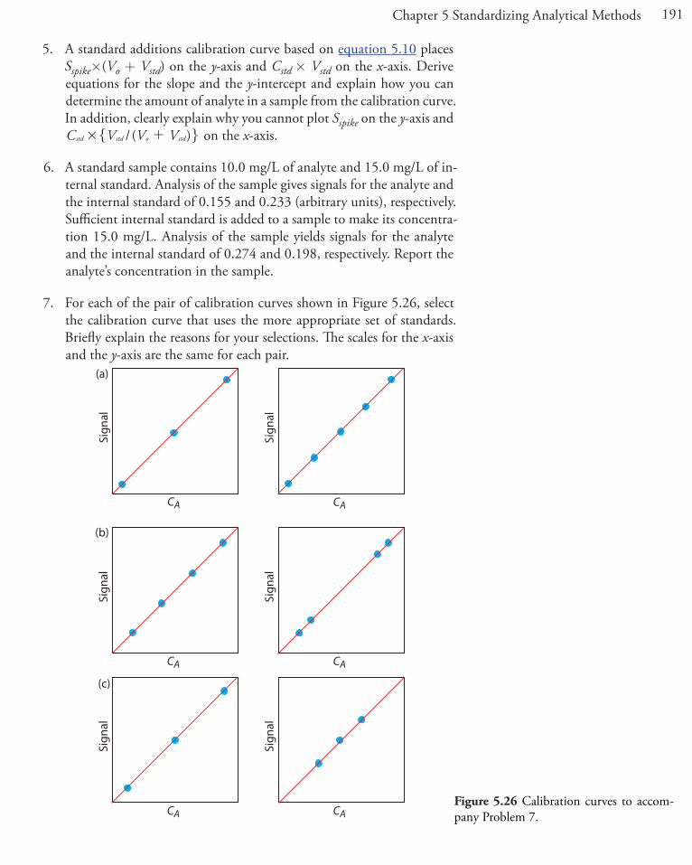
191Chapter 5 Standardizing Analytical Methods
5. A standard additions calibration curve based on equation 5.10 places Sspike×(Vo + Vstd) on the y-axis and Cstd × Vstd on the x-axis. Derive equations for the slope and the y-intercept and explain how you can determine the amount of analyte in a sample from the calibration curve. In addition, clearly explain why you cannot plot Sspike on the y-axis and
/ ( )C V V Vstd std o std# +" , on the x-axis.
6. A standard sample contains 10.0 mg/L of analyte and 15.0 mg/L of in-ternal standard. Analysis of the sample gives signals for the analyte and the internal standard of 0.155 and 0.233 (arbitrary units), respectively. Sufficient internal standard is added to a sample to make its concentra-tion 15.0 mg/L. Analysis of the sample yields signals for the analyte and the internal standard of 0.274 and 0.198, respectively. Report the analyte’s concentration in the sample.
7. For each of the pair of calibration curves shown in Figure 5.26, select the calibration curve that uses the more appropriate set of standards. Briefly explain the reasons for your selections. The scales for the x-axis and the y-axis are the same for each pair.
Sign
al
CA
Sign
al
CA
Sign
al
CA
Sign
al
CA
Sign
al
CA
Sign
al
CA
(a)
(b)
(c)
Figure 5.26 Calibration curves to accom-pany Problem 7.

192 Analytical Chemistry 2.1
8. The following data are for a series of external standards of Cd2+ buffered to a pH of 4.6.14
[Cd2+] (nM) 15.4 30.4 44.9 59.0 72.7 86.0Sspike (nA) 4.8 11.4 18.2 26.6 32.3 37.7
(a) Use a linear regression analysis to determine the equation for the calibration curve and report confidence intervals for the slope and the y-intercept.
(b) Construct a plot of the residuals and comment on their significance.
At a pH of 3.7 the following data were recorded for the same set of external standards.
[Cd2+] (nM) 15.4 30.4 44.9 59.0 72.7 86.0
Sspike (nA) 15.0 42.7 58.5 77.0 101 118
(c) How much more or less sensitive is this method at the lower pH?
(d) A single sample is buffered to a pH of 3.7 and analyzed for cadmium, yielding a signal of 66.3 nA. Report the concentration of Cd2+ in the sample and its 95% confidence interval.
9. To determine the concentration of analyte in a sample, a standard ad-dition is performed. A 5.00-mL portion of sample is analyzed and then successive 0.10-mL spikes of a 600.0 ppb standard of the analyte are added, analyzing after each spike. The following table shows the results of this analysis.
Vspike (mL) 0.00 0.10 0.20 0.30
Stotal (arbitrary units) 0.119 0.231 0.339 0.442
Construct an appropriate standard additions calibration curve and use a linear regression analysis to determine the concentration of analyte in the original sample and its 95% confidence interval.
10. Troost and Olavsesn investigated the application of an internal stan-dardization to the quantitative analysis of polynuclear aromatic hy-drocarbons.15 The following results were obtained for the analysis of phenanthrene using isotopically labeled phenanthrene as an internal standard. Each solution was analyzed twice.
CA/CIS 0.50 1.25 2.00 3.00 4.00
SA/SIS0.5140.522
0.9931.024
1.4861.471
2.0442.080
2.3422.550
14 Wojciechowski, M.; Balcerzak, J. Anal. Chim. Acta 1991, 249, 433–445.15 Troost, J. R.; Olavesen, E. Y. Anal. Chem. 1996, 68, 708–711.

193Chapter 5 Standardizing Analytical Methods
(a) Determine the equation for the calibration curve using a linear regression, and report confidence intervals for the slope and the y-intercept. Average the replicate signals for each standard before you complete the linear regression analysis.
(b) Based on your results explain why the authors concluded that the internal standardization was inappropriate.
11. In Chapter 4 we used a paired t-test to compare two analytical methods that were used to analyze independently a series of samples of vari-able composition. An alternative approach is to plot the results for one method versus the results for the other method. If the two methods yield identical results, then the plot should have an expected slope, b1, of 1.00 and an expected y-intercept, b0, of 0.0. We can use a t-test to compare the slope and the y-intercept from a linear regression to the ex-pected values. The appropriate test statistic for the y-intercept is found by rearranging equation 5.23.
t sb
sb
expb b
0 0 0
0 0
b=
-=
Rearranging equation 5.22 gives the test statistic for the slope.
t sb
sb1
expb b
1 1 1
1 1
b=
-=
-
Reevaluate the data in problem 25 from Chapter 4 using the same significance level as in the original problem.
12. Consider the following three data sets, each of which gives values of y for the same values of x.
Data Set 1 Data Set 2 Data Set 3x y1 y2 y3
10.00 8.04 9.14 7.468.00 6.95 8.14 6.77
13.00 7.58 8.74 12.749.00 8.81 8.77 7.11
11.00 8.33 9.26 7.8114.00 9.96 8.10 8.84
6.00 7.24 6.13 6.084.00 4.26 3.10 5.39
12.00 10.84 9.13 8.157.00 4.82 7.26 6.425.00 5.68 4.74 5.73
Although this is a common approach for comparing two analytical methods, it does violate one of the requirements for an unweighted linear regression—that in-determinate errors affect y only. Because indeterminate errors affect both analytical methods, the result of an unweighted lin-ear regression is biased. More specifically, the regression underestimates the slope, b1, and overestimates the y-intercept, b0. We can minimize the effect of this bias by placing the more precise analytical meth-od on the x-axis, by using more samples to increase the degrees of freedom, and by using samples that uniformly cover the range of concentrations.
For more information, see Miller, J. C.; Miller, J. N. Statistics for Analytical Chem-istry, 3rd ed. Ellis Horwood PTR Pren-tice-Hall: New York, 1993. Alternative approaches are found in Hartman, C.; Smeyers-Verbeke, J.; Penninckx, W.; Mas-sart, D. L. Anal. Chim. Acta 1997, 338, 19–40, and Zwanziger, H. W.; Sârbu, C. Anal. Chem. 1998, 70, 1277–1280.
These three data sets are taken from Ans-combe, F. J. “Graphs in Statistical Analy-sis,” Amer. Statis. 1973, 27, 17-21.

194 Analytical Chemistry 2.1
(a) An unweighted linear regression analysis for the three data sets gives nearly identical results. To three significant figures, each data set has a slope of 0.500 and a y-intercept of 3.00. The standard devia-tions in the slope and the y-intercept are 0.118 and 1.125 for each data set. All three standard deviations about the regression are 1.24. Based on these results for a linear regression analysis, comment on the similarity of the data sets.
(b) Complete a linear regression analysis for each data set and verify that the results from part (a) are correct. Construct a residual plot for each data set. Do these plots change your conclusion from part (a)? Explain.
(c) Plot each data set along with the regression line and comment on your results.
(d) Data set 3 appears to contain an outlier. Remove the apparent out-lier and reanalyze the data using a linear regression. Comment on your result.
(e) Briefly comment on the importance of visually examining your data.
13. Fanke and co-workers evaluated a standard additions method for a voltammetric determination of Tl.16 A summary of their results is tabu-lated in the following table.
ppm Tl added Instrument Response (mA)
0.000 2.53 2.50 2.70 2.63 2.70 2.80 2.520.387 8.42 7.96 8.54 8.18 7.70 8.34 7.981.851 29.65 28.70 29.05 28.30 29.20 29.95 28.955.734 84.8 85.6 86.0 85.2 84.2 86.4 87.8
Use a weighted linear regression to determine the standardization rela-tionship for this data.
5J Solutions to Practice ExercisesPractice Exercise 5.1Substituting the sample’s absorbance into the calibration equation and solving for CA give
Ssamp = 0.114 = 29.59 M–1 × CA + 0.015
CA = 3.35 × 10⁻³ M
For the one-point standardization, we first solve for kA16 Franke, J. P.; de Zeeuw, R. A.; Hakkert, R. Anal. Chem. 1978, 50, 1374–1380.

195Chapter 5 Standardizing Analytical Methods
.. .k C
S3 16 10
0 0931 29 46M MAstd
std3
1
#= = =-
-
and then use this value of kA to solve for CA.
.. .C k
S29 46
0 114 3 87 10M MAA
samp1
3#= = =--
When using multiple standards, the indeterminate errors that affect the signal for one standard are partially compensated for by the indeterminate errors that affect the other standards. The standard selected for the one-point standardization has a signal that is smaller than that predicted by the regression equation, which underestimates kA and overestimates CA.
Click here to return to the chapter.
Practice Exercise 5.2We begin with equation 5.8
S k C VV C V
Vspike A A
f
ostd
f
std= +a krewriting it as
Vk C V k C V
V0f
A A oA std
f
std#= + & 0which is in the form of the linear equation
y = y-intercept + slope × x
where y is Sspike and x is Cstd × Vstd/Vf. The slope of the line, therefore, is kA, and the y-intercept is kACAVo/Vf. The x-intercept is the value of x when y is zero, or
Vk C V k x0 -intercept
f
A A oA #= + " ,
x kk C V V
VC V-intercept
A
A A o f
f
A o=- =-
Click here to return to the chapter.
Practice Exercise 5.3Using the calibration equation from Figure 5.7a, we find that the x-in-tercept is
.. .x 0 0854
0 1478 1 731intercept mL mL1- =- =--
If we plug this result into the equation for the x-intercept and solve for CA, we find that the concentration of Mn2+ is
( ).
( . ) ..V
x CC 25 00
1 731 100 66 96
-interceptmL
mL mg/Lmg/L
o
stdA
#=- -
-==
For Figure 7b, the x-intercept is

196 Analytical Chemistry 2.1
.. .intx ercept 0 04250 1478 3 478- mL/mg mg/mL=- =-
and the concentration of Mn2+ is( )
.( . / ) .
.C Vx V
25 003 478 50 00
6 96-intercept
mLmg mL mL
mg/LAo
f #=- =-
-=
Click here to return to the chapter.
Practice Exercise 5.4We begin by setting up a table to help us organize the calculation.
xi yi xiyi xi2
0.000 0.00 0.000 0.000
1.55×10⁻³ 0.050 7.750×10⁻⁵ 2.403×10⁻⁶
3.16×10⁻³ 0.093 2.939×10⁻⁴ 9.986×10⁻⁶
4.74×10⁻³ 0.143 6.778×10⁻⁴ 2.247×10⁻⁵
6.34×10⁻³ 0.188 1.192×10⁻³ 4.020×10⁻⁵
7.92×10⁻³ 0.236 1.869×10⁻³ 6.273×10⁻⁵
Adding the values in each column gives
. .x y2 371 10 0 710ii
n
ii
n
1
2
1#= =
=
-
=
/ /
. .x y x4 110 10 1 378 10i ii
n
ii
n
1
3 2
1
4# #= ==
-
=
-/ /When we substitute these values into equation 5.17 and equation 5.18, we find that the slope and the y-intercept are
( . ) ( . )( . ) ( . ) ( . ) .b 6 1 378 10 2 371 10
6 4 110 10 2 371 10 0 710 29 571 4 2 2
3 2
# # ## # # #
=-
-=- -
- -
. . ( . ) .b 60 710 29 57 2 371 10 0 00150
2# #=
-=
-
and that the regression equation is
Sstd = 29.57 × Cstd + 0.0015
To calculate the 95% confidence intervals, we first need to determine the standard deviation about the regression. The following table helps us organize the calculation.
xi yi yiV ( )y yi i
2-V0.000 0.00 0.0015 2.250×10⁻⁶
1.55×10⁻³ 0.050 0.0473 7.110×10⁻⁶
3.16×10⁻³ 0.093 0.0949 3.768×10⁻⁶
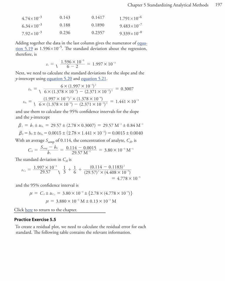
197Chapter 5 Standardizing Analytical Methods
4.74×10⁻³ 0.143 0.1417 1.791×10⁻⁶
6.34×10⁻³ 0.188 0.1890 9.483×10⁻⁷
7.92×10⁻³ 0.236 0.2357 9.339×10⁻⁸
Adding together the data in the last column gives the numerator of equa-tion 5.19 as 1.596×10⁻⁵. The standard deviation about the regression, therefore, is
. .s 6 21 596 10 1 997 10r
53# #=
-=
--
Next, we need to calculate the standard deviations for the slope and the y-intercept using equation 5.20 and equation 5.21.
( . ) ( . )( . ) .s 6 1 378 10 2 371 10
6 1 997 10 0 3007b 4 2 2
3 2
1 # # ## #
=-
=- -
-
( . ) ( . )( . ) ( . ) .s 6 1 378 10 2 371 101 997 10 1 378 10 1 441 10b 4 2 2
3 2 43
0 # # ## # #
#=-
=- -
- --
and use them to calculate the 95% confidence intervals for the slope and the y-intercept
. ( . . ) . .b ts 29 57 2 78 0 3007 29 57 0 84M Mb1 11 1
1! ! # !b = = = - -
. ( . ) .. .b ts 0 0015 2 78 0 00151 441 10 0 0040b0 03
0! ! # !#b = = =-
With an average Ssamp of 0.114, the concentration of analyte, CA, is
.. . .C b
S b29 57
0 114 0 0015 3 80 10M MAsamp
1
01
3 1#=-
= - =-- -
The standard deviation in CA is
..
( . ) ( . )( . . )
.
s 29 571 997 10
31
61
29 57 4 408 100 114 0 1183
4 778 10
C
3
2 5
2
5
A
## #
#
= + +-
=
-
-
-
and the 95% confidence interval is
. . ( . )C ts 3 80 10 2 78 4 778 10A C3 5
A! # ! # #n= = - -" ,. .3 880 10 0 13 10M M3 3# ! #n= - -
Click here to return to the chapter.
Practice Exercise 5.5To create a residual plot, we need to calculate the residual error for each standard. The following table contains the relevant information.

198 Analytical Chemistry 2.1
xi yi yiV y yi i-V
0.000 0.00 0.0015 –0.0015
1.55×10⁻³ 0.050 0.0473 0.0027
3.16×10⁻³ 0.093 0.0949 –0.0019
4.74×10⁻³ 0.143 0.1417 0.0013
6.34×10⁻³ 0.188 0.1890 –0.0010
7.92×10⁻³ 0.236 0.2357 0.0003
Figure 5.27 shows a plot of the resulting residual errors. The residual er-rors appear random, although they do alternate in sign, and that do not show any significant dependence on the analyte’s concentration. Taken together, these observations suggest that our regression model is appro-priate.
Click here to return to the chapter
Practice Exercise 5.6Begin by entering the data into an Excel spreadsheet, following the format shown in Figure 5.15. Because Excel’s Data Analysis tools provide most of the information we need, we will use it here. The resulting output, which is shown in Figure 5.28, provides the slope and the y-intercept, along with their respective 95% confidence intervals. Excel does not provide a function for calculating the uncertainty in the analyte’s concentration, CA, given the signal for a sample, Ssamp. You must complete these calculations by hand. With an Ssamp of 0.114, we find that CA is
.. . .C b
S b29 59
0 114 0 0014 3 80 10M MAsamp
1
01
3#=-
= - =--
The standard deviation in CA is
Figure 5.27 Plot of the residual errors for the data in Practice Exercise 5.5.
0.000 0.002 0.004 0.006 0.008
-0.010
0.000
0.010
resi
dual
err
or
CA
Figure 5.28 Excel’s summary of the regression results for Practice Exercise 5.6.
SUMMARY OUTPUT
Regression StatisticsMultiple R 0.99979366R Square 0.99958737Adjusted R Square0.99948421Standard Error 0.00199602Observations 6
ANOVAdf SS MS F Significance F
Regression 1 0.0386054 0.0386054 9689.9103 6.3858E-08Residual 4 1.5936E-05 3.9841E-06Total 5 0.03862133
Coefficients Standard Error t Stat P-value Lower 95% Upper 95% Lower 95.0% Upper 95.0%Intercept 0.00139272 0.00144059 0.96677158 0.38840479 -0.00260699 0.00539242 -0.00260699 0.00539242Cstd 29.5927329 0.30062507 98.437342 6.3858E-08 28.7580639 30.4274019 28.7580639 30.4274019

199Chapter 5 Standardizing Analytical Methods
..
( . ) ( . )( . . )
.
s 29 591 996 10
31
61
29 59 4 408 100 114 0 1183
4 772 10
C
3
2 5
2
5
A
## #
#
= + +-
=
-
-
-
and the 95% confidence interval is
. . ( . )C ts 3 80 10 2 78 4 772 10A C3 5
A! # ! # #n= = - -" ,. .3 80 10 0 13 10M M3 3# ! #n= - -
Click here to return to the chapter
Practice Exercise 5.7Figure 5.29 shows the R session for this problem, including loading the chemCal package, creating objects to hold the values for Cstd, Sstd, and Ssamp. Note that for Ssamp, we do not have the actual values for the three replicate measurements. In place of the actual measurements, we just en-ter the average signal three times. This is okay because the calculation depends on the average signal and the number of replicates, and not on the individual measurements.
Click here to return to the chapter
> library("chemCal")> conc=c(0, 1.55e-3, 3.16e-3, 4.74e-3, 6.34e-3, 7.92e-3)> signal=c(0, 0.050, 0.093, 0.143, 0.188, 0.236)> model=lm(signal~conc)> summary(model)
Call:lm(formula = signal ~ conc)
Residuals: 1 2 3 4 5 6 -0.0013927 0.0027385 -0.0019058 0.0013377 -0.0010106 0.0002328
Coe�cients: Estimate Std. Error t value Pr(>|t|) (Intercept) 0.001393 0.001441 0.967 0.388 conc 29.592733 0.300625 98.437 6.39e-08 ***---Signif. codes: 0 ‘***’ 0.001 ‘**’ 0.01 ‘*’ 0.05 ‘.’ 0.1 ‘ ’ 1
Residual standard error: 0.001996 on 4 degrees of freedomMultiple R-Squared: 0.9996, Adjusted R-squared: 0.9995 F-statistic: 9690 on 1 and 4 DF, p-value: 6.386e-08
> samp=c(0.114, 0.114, 0.114)> inverse.predict(model,samp,alpha=0.05)$Prediction[1] 0.003805234
$`Standard Error`[1] 4.771723e-05
$Con�dence[1] 0.0001324843
$`Con�dence Limits`[1] 0.003672750 0.003937719
Figure 5.29 R session for completing Practice Exercise 5.7.

200 Analytical Chemistry 2.1