chapter 15dpuadweb.depauw.edu/harvey_web/etextproject/ac2.1files/chapter15.pdf954 analytical...

953

Chapter 15

Quality AssuranceChapter Overview15A The Analytical Perspective—Revisited15B Quality Control15C Quality Assessment15D Evaluating Quality Assurance Data15E Key Terms15F Chapter Summary15G Problems15H Solutions to Practice Exercises

In Chapter 14 we discussed the process of developing a standard method, including optimizing the experimental procedure, verifying that the method produces acceptable precision and accuracy in the hands of a signal analyst, and validating the method for general use by the broader analytical community. Knowing that a method meets suitable standards is important if we are to have confidence in our results. Even so, using a standard method does not guarantee that the result of an analysis is acceptable. In this chapter we introduce the quality assurance procedures used in industry and government labs for the real-time monitoring of routine chemical analyses.

954 Analytical Chemistry 2.1

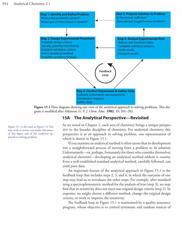
15A The Analytical Perspective—RevisitedAs we noted in Chapter 1, each area of chemistry brings a unique perspec-tive to the broader discipline of chemistry. For analytical chemistry this perspective is as an approach to solving problem, one representation of which is shown in Figure 15.1.

If you examine an analytical method it often seems that its development was a straightforward process of moving from a problem to its solution. Unfortunately—or, perhaps, fortunately for those who consider themselves analytical chemists!—developing an analytical method seldom is routine. Even a well-established standard analytical method, carefully followed, can yield poor data.

An important feature of the analytical approach in Figure 15.1 is the feedback loop that includes steps 2, 3, and 4, in which the outcome of one step may lead us to reevaluate the other steps. For example, after standard-izing a spectrophotometric method for the analysis of iron (step 3), we may find that its sensitivity does not meet our original design criteria (step 2). In response, we might choose a different method, change the original design criteria, or work to improve the sensitivity.

The feedback loop in Figure 15.1 is maintained by a quality assurance program, whose objective is to control systematic and random sources of

Figure 15.1 Flow diagram showing one view of the analytical approach to solving problems. This dia-gram is modified after Atkinson, G. F. J. Chem. Educ. 1982, 59, 201–202.

Figure 15.1 is the same as Figure 1.3. You may wish to review our earlier discussion of this figure and of the analytical ap-proach to solving problem.

Step 1. Identify and De�ne Problem What is the problem’s context?What type of information is needed?

Step 5. Propose Solution to ProblemIs the answer su�cient?Does answer suggest a new problem?

Step 2. Design Experimental Procedure Establish design criteria.Identify potential interferents.Establish validation criteria.Select analytical method.Establish sampling strategy.

Step 4. Analyze Experimental DataReduce and transform data.Complete statistical analysis.Verify results.Interpret results.

Step 3. Conduct Experiment & Gather DataCalibrate instruments and equipment.Standardize reagents.Gather data.

FeedbackLoop

955Chapter 15 Quality Assurance

error.1 The underlying assumption of a quality assurance program is that results obtained when an analysis is under statistical control are free of bias and are characterized by well-defined confidence intervals. When used properly, a quality assurance program identifies the practices necessary to bring a system into statistical control, allows us to determine if the system remains in statistical control, and suggests a course of corrective action if the system falls out of statistical control.

The focus of this chapter is on the two principal components of a qual-ity assurance program: quality control and quality assessment. In ad-dition, we will give considerable attention to the use of control charts for monitoring the quality of analytical data.

15B Quality ControlQuality control encompasses all activities that bring an analysis into sta-tistical control. The most important facet of quality control is a set of writ-ten directives that describe relevant laboratory-specific, technique-specific, sample-specific, method-specific, and protocol-specific operations. Good laboratory practices (GLPs) describe the general laboratory operations that we must follow in any analysis. These practices include properly re-cording data and maintaining records, using chain-of-custody forms for samples, specifying and purifying chemical reagents, preparing commonly used reagents, cleaning and calibrating glassware, training laboratory per-sonnel, and maintaining the laboratory facilities and general laboratory equipment.

Good measurement practices (GMPs) describe those operations spe-cific to a technique. In general, GMPs provide instructions for maintain-ing, calibrating, and using equipment and instrumentation. For example, a GMP for a titration describes how to calibrate the buret (if required), how to fill the buret with titrant, the correct way to read the volume of titrant in the buret, and the correct way to dispense the titrant.

The directions for analyzing a specific analyte in a specific matrix are described by a standard operations procedure (SOP). The SOP indi-cates how we process the sample in the laboratory, how we separate the analyte from potential interferents, how we standardize the method, how we measure the analytical signal, how we transform the data into the desired result, and how we use quality assessment tools to maintain quality control. If the laboratory is responsible for sampling, then the SOP also states how we must collect, process, and preserve the sample in the field. An SOP may be developed and used by a single laboratory, or it may be a standard procedure approved by an organization such as the American Society for

1 (a) Taylor, J. K. Anal. Chem. 1981, 53, 1588A–1596A; (b) Taylor, J. K. Anal. Chem. 1983, 55, 600A–608A; (c) Taylor, J. K. Am. Lab October 1985, 53, 67–75; (d) Nadkarni, R. A. Anal. Chem. 1991, 63, 675A–682A; (e) Valcárcel, M.; Ríos, A. Trends Anal. Chem. 1994, 13, 17–23.

For one example of quality control, see Keith, L. H.; Crummett, W.; Deegan, J., Jr.; Libby, R. A.; Taylor, J. K.; Wentler, G. “Principles of Environmental Analysis,” Anal. Chem. 1983, 55, 2210–2218. This article describes guidelines developed by the Subcommittee on Environmental An-alytical Chemistry, a subcommittee of the American Chemical Society’s Committee on Environmental Improvement.

An analysis is in a state of statistical con-trol when it is reproducible and free from bias.


Testing Materials or the Federal Food and Drug Administration. A typical SOP is provided in the following example.

Example 15.1

Provide an SOP for the determination of cadmium in lake sediments using atomic absorption spectroscopy and a normal calibration curve.

SolutionCollect sediment samples using a bottom grab sampler and store them at 4 oC in acid-washed polyethylene bottles during transportation to the laboratory. Dry the samples to constant weight at 105

oC and grind them to a uniform particle size. Extract the cadmium in a 1-g sample of sediment by adding the sediment and 25 mL of 0.5 M HCl to an acid-washed 100-mL polyethylene bottle and shaking for 24 h. After filtering, analyze the sample by atomic absorption spectroscopy using an air–acetylene flame, a wavelength of 228.8 nm, and a slit width of 0.5 nm. Prepare a normal calibration curve using five standards with nominal concentrations of 0.20, 0.50, 1.00, 2.00, and 3.00 ppm. Periodically check the accuracy of the calibration curve by analyzing the 1.00-ppm standard. An accuracy of ±10% is considered acceptable.

Although an SOP provides a written procedure, it is not necessary to follow the procedure exactly as long as we are careful to identify any modi-fications. On the other hand, we must follow all instructions in a protocol for a specific purpose (PSP)—the most detailed of the written quality control directives—before an agency or a client will accept our results. In many cases the required elements of a PSP are established by the agency that sponsors the analysis. For example, a lab working under contract with the Environmental Protection Agency must develop a PSP that addresses such items as sampling and sample custody, frequency of calibration, schedules for the preventive maintenance of equipment and instrumentation, and management of the quality assurance program.

Two additional aspects of a quality control program deserve mention. The first is that the individuals responsible for collecting and analyzing the samples can critically examine and reject individual samples, measure-ments, and results. For example, when analyzing sediments for cadmium (see the SOP in Example 15.1) we might choose to screen sediment samples, discarding a sample that contains foreign objects—such as rocks, twigs, or trash—replacing it with an additional sample. If we observe a sudden change in the performance of the atomic absorption spectrometer, we may choose to reanalyze the affected samples. We may also decide to reanalyze a sample if the result of its analysis clearly is unreasonable. By identifying those samples, measurements, and results subject to gross systematic errors, inspection helps control the quality of an analysis.

Figure 7.7 in Chapter 7 shows an example of a bottom grab sampler.


The second additional consideration is the certification of an analyst’s competence to perform the analysis for which he or she is responsible. Be-fore an analyst is allowed to perform a new analytical method, he or she may be required to analyze successfully an independent check sample with acceptable accuracy and precision. The check sample is similar in composi-tion to samples that the analyst will analyze later, with a concentration that is 5 to 50 times that of the method’s detection limit.

15C Quality AssessmentThe written directives of a quality control program are a necessary, but not a sufficient condition for obtaining and maintaining a state of statistical control. Although quality control directives explain how to conduct an analysis, they do not indicate whether the system is under statistical control. This is the role of quality assessment, the second component of a quality assurance program.

The goals of quality assessment are to determine when an analysis has reached a state of statistical control, to detect when an analysis falls out of statistical control, and to suggest possible reasons for this loss of statistical control. For convenience, we divide quality assessment into two categories: internal methods coordinated within the laboratory, and external methods organized and maintained by an outside agency.

15C.1 Internal Methods of Quality Assessment

The most useful methods for quality assessment are those coordinated by the laboratory, which provide immediate feedback about the analytical method’s state of statistical control. Internal methods of quality assessment include the analysis of duplicate samples, the analysis of blanks, the analysis of standard samples, and spike recoveries.

AnAlysis of DuplicAte sAmples

An effective method for determining the precision of an analysis is to an-alyze duplicate samples. Duplicate samples are obtained by dividing a single gross sample into two parts, although in some cases the duplicate samples are independently collected gross samples. We report the results for the duplicate samples, X1 and X2, by determining the difference, d, or the relative difference, (d)r, between the two samples

d X X1 2= -

( ) ( ) /d X Xd

2 100r1 2

#=+

and comparing to an accepted value, such as those in Table 15.1 for the analysis of waters and wastewaters. Alternatively, we can estimate the stan-dard deviation using the results for a set of n duplicates

A split sample is another name for dupli-cate samples created from a single gross sample.


s n

d

2i

i

n2

1= =

/

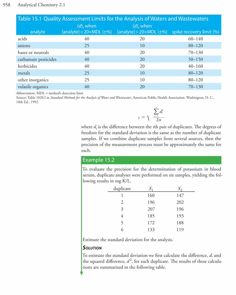
where di is the difference between the ith pair of duplicates. The degrees of freedom for the standard deviation is the same as the number of duplicate samples. If we combine duplicate samples from several sources, then the precision of the measurement process must be approximately the same for each.

Example 15.2

To evaluate the precision for the determination of potassium in blood serum, duplicate analyses were performed on six samples, yielding the fol-lowing results in mg K/L.

duplicate X1 X21 160 1472 196 2023 207 1964 185 1935 172 1886 133 119

Estimate the standard deviation for the analysis.

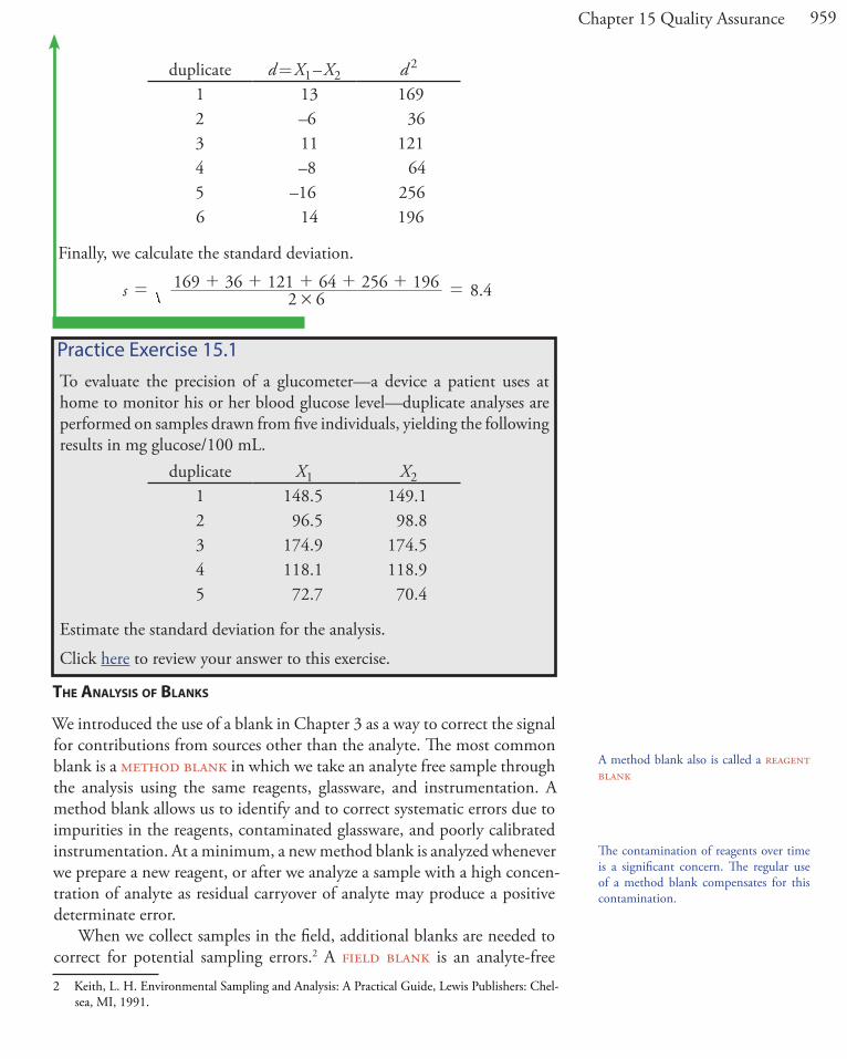
SolutionTo estimate the standard deviation we first calculate the difference, d, and the squared difference, d 2, for each duplicate. The results of these calcula-tions are summarized in the following table.

Table 15.1 Quality Assessment Limits for the Analysis of Waters and Wastewaters

analyte(d)r when

[analyte] < 20�MDL (±%)(d)r when

[analyte] > 20�MDL (±%) spike recovery limit (%)acids 40 20 60–140anions 25 10 80–120bases or neutrals 40 20 70–130carbamate pesticides 40 20 50–150herbicides 40 20 40–160metals 25 10 80–120other inorganics 25 10 80–120volatile organics 40 20 70–130

Abbreviation: MDL = method’s detection limitSource: Table 1020.I in Standard Methods for the Analysis of Water and Wastewater, American Public Health Association: Washington, D. C., 18th Ed., 1992.


duplicate d = X1 – X2 d 2

1 13 1692 –6 363 11 1214 –8 645 –16 2566 14 196

Finally, we calculate the standard deviation.

.s 2 6169 36 121 64 256 196 8 4

#= + + + + + =

The contamination of reagents over time is a significant concern. The regular use of a method blank compensates for this contamination.

A method blank also is called a reagent blank

Practice Exercise 15.1To evaluate the precision of a glucometer—a device a patient uses at home to monitor his or her blood glucose level—duplicate analyses are performed on samples drawn from five individuals, yielding the following results in mg glucose/100 mL.

duplicate X1 X21 148.5 149.12 96.5 98.83 174.9 174.54 118.1 118.95 72.7 70.4

Estimate the standard deviation for the analysis.

Click here to review your answer to this exercise.

the AnAlysis of BlAnks

We introduced the use of a blank in Chapter 3 as a way to correct the signal for contributions from sources other than the analyte. The most common blank is a method blank in which we take an analyte free sample through the analysis using the same reagents, glassware, and instrumentation. A method blank allows us to identify and to correct systematic errors due to impurities in the reagents, contaminated glassware, and poorly calibrated instrumentation. At a minimum, a new method blank is analyzed whenever we prepare a new reagent, or after we analyze a sample with a high concen-tration of analyte as residual carryover of analyte may produce a positive determinate error.

When we collect samples in the field, additional blanks are needed to correct for potential sampling errors.2 A field blank is an analyte-free 2 Keith, L. H. Environmental Sampling and Analysis: A Practical Guide, Lewis Publishers: Chel-

sea, MI, 1991.


sample carried from the laboratory to the sampling site. At the sampling site the blank is transferred to a clean sample container, which exposes it to the local environment. The field blank is then preserved and transported back to the laboratory for analysis. A field blank helps identify systematic errors due to sampling, transport, and analysis. A trip blank is an analyte-free sample carried from the laboratory to the sampling site and back to the laboratory without being opened. A trip blank helps to identify systematic errors due to cross-contamination of volatile organic compounds during transport, handling, storage, and analysis.

AnAlysis of stAnDArDs

Another tool for monitoring an analytical method’s state of statistical con-trol is to analyze a standard that contains a known concentration of analyte. A standard reference material (SRM) is the ideal choice, provided that the SRM’s matrix is similar to that of our samples. A variety of SRMs are avail-able from the National Institute of Standards and Technology (NIST). If a suitable SRM is not available, then we can use an independently prepared synthetic sample if it is prepared from reagents of known purity. In all cases, the analyte’s experimentally determined concentration in the standard must fall within predetermined limits before the analysis is considered under statistical control.

spike recoveries

One of the most important quality assessment tools is the recovery of a known addition, or spike, of analyte to a method blank, a field blank, or a sample. To determine a spike recovery, the blank or sample is split into two portions and a known amount of a standard solution of analyte is added to one portion. The analyte’s concentration is determined for both the spiked, F, and unspiked portions, I, and the percent recovery, %R, is calculated as

%R AF I 100#= -

where A is the concentration of analyte added to the spiked portion.

Example 15.3

A spike recovery for the analysis of chloride in well water was performed by adding 5.00 mL of a 250.0 ppm solution of Cl– to a 50-mL volumet-ric flask and diluting to volume with the sample. An unspiked sample was prepared by adding 5.00 mL of distilled water to a separate 50-mL volumetric flask and diluting to volume with the sample. Analysis of the sample and the spiked sample return chloride concentrations of 18.3 ppm and 40.9 ppm, respectively. Determine the spike recovery.

Table 4.7 in Chapter 4 provides a sum-mary of SRM 2346, a standard sample of Gingko biloba leaves with certified values for the concentrations of flavonoids, ter-pene ketones, and toxic elements, such as mercury and lead.


SolutionTo calculate the concentration of the analyte added in the spike, we take into account the effect of dilution.

. .. .A 250 0 50 0

5 00 25 0ppm mLmL ppm#= =

Thus, the spike recovery is

% .. . . %R 25 0

40 9 18 3 100 90 4#= - =

Practice Exercise 15.2To test a glucometer, a spike recovery is carried out by measuring the amount of glucose in a sample of a patient’s blood before and after spiking it with a standard solution of glucose. Before spiking the sam-ple the glucose level is 86.7 mg/100 mL and after spiking the sample it is 110.3 mg/100 mL. The spike is prepared by adding 10.0 µL of a 25 000 mg/100mL standard to a 10.0-mL portion of the blood. What is the spike recovery for this sample.


We can use a spike recovery on a method blank and a field blank to evaluate the general performance of an analytical procedure. A known con-centration of analyte is added to each blank at a concentration that is 5 to 50 times the method’s detection limit. A systematic error during sampling and transport will result in an unacceptable recovery for the field blank, but not for the method blank. A systematic error in the laboratory, however, affects the recoveries for both the field blank and the method blank.

Spike recoveries on a sample are used to detect systematic errors due to the sample’s matrix, or to evaluate the stability of a sample after its collec-tion. Ideally, samples are spiked in the field at a concentration that is 1 to 10 times the analyte’s expected concentration or 5 to 50 times the method’s detection limit, whichever is larger. If the recovery for a field spike is unac-ceptable, then a duplicate sample is spiked in the laboratory and analyzed immediately. If the laboratory spike’s recovery is acceptable, then the poor recovery for the field spike likely is the result of the sample’s deterioration during storage. If the recovery for the laboratory spike also is unacceptable, the most probable cause is a matrix-dependent relationship between the analytical signal and the analyte’s concentration. In this case the sample is analyzed by the method of standard additions. Typical limits for spike re-coveries for the analysis of waters and wastewaters are shown in Table 15.1.

15C.2 External Methods of Quality Assessment

Internal methods of quality assessment always carry some level of suspi-cion because there is a potential for bias in their execution and interpre-

Figure 15.2, which we will discuss in Section 15D, illustrates the use of spike recoveries as part of a quality assessment program.


tation. For this reason, external methods of quality assessment also play an important role in a quality assurance program. One external method of quality assessment is the certification of a laboratory by a sponsoring agency. Certification of a lab is based on its successful analysis of a set of proficiency standards prepared by the sponsoring agency. For example, laboratories involved in environmental analyses may be required to analyze standard samples prepared by the Environmental Protection Agency. A sec-ond example of an external method of quality assessment is a laboratory’s voluntary participation in a collaborative test sponsored by a professional organization, such as the Association of Official Analytical Chemists. Fi-nally, an individual contracting with a laboratory can perform his or her own external quality assessment by submitting blind duplicate samples and blind standards to the laboratory for analysis. If the results for the quality assessment samples are unacceptable, then there is good reason to question the laboratory’s results for other samples.

15D Evaluating Quality Assurance DataIn the previous section we described several internal methods of quality assessment that provide quantitative estimates of the systematic errors and the random errors in an analytical method. Now we turn our attention to how we incorporate this quality assessment data into a complete qual-ity assurance program. There are two general approaches to developing a quality assurance program: a prescriptive approach, in which we prescribe an exact method of quality assessment, and a performance-based approach in which we can use any form of quality assessment, provided that we can demonstrate an acceptable level of statistical control.3

15D.1 Prescriptive Approach

With a prescriptive approach to quality assessment, duplicate samples, blanks, standards, and spike recoveries are measured using a specific proto-col. We compare the result of each analysis to a single predetermined limit, taking an appropriate corrective action if the limit is exceeded. Prescriptive approaches to quality assurance are common for programs and laboratories subject to federal regulation. For example, the Food and Drug Administra-tion (FDA) specifies quality assurance practices that must be followed by laboratories that analyze products regulated by the FDA.

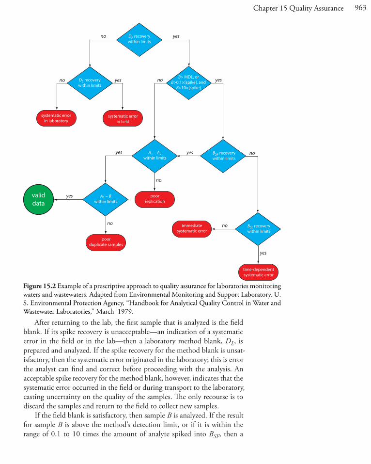
Figure 15.2 provides a typical example of a prescriptive approach to quality assessment. Two samples, A and B, are collected at the sample site. Sample A is split into two equal-volume samples, A1 and A2. Sample B is also split into two equal-volume samples, one of which, BSF, is spiked in the field with a known amount of analyte. A field blank, DF, also is spiked with the same amount of analyte. All five samples (A1, A2, B, BSF, and DF) are preserved if necessary and transported to the laboratory for analysis.

3 Poppiti, J. Environ. Sci. Technol. 1994, 28, 151A–152A.

See Chapter 14 for a more detailed de-scription of collaborative testing.


After returning to the lab, the first sample that is analyzed is the field blank. If its spike recovery is unacceptable—an indication of a systematic error in the field or in the lab—then a laboratory method blank, DL, is prepared and analyzed. If the spike recovery for the method blank is unsat-isfactory, then the systematic error originated in the laboratory; this is error the analyst can find and correct before proceeding with the analysis. An acceptable spike recovery for the method blank, however, indicates that the systematic error occurred in the field or during transport to the laboratory, casting uncertainty on the quality of the samples. The only recourse is to discard the samples and return to the field to collect new samples.

If the field blank is satisfactory, then sample B is analyzed. If the result for sample B is above the method’s detection limit, or if it is within the range of 0.1 to 10 times the amount of analyte spiked into BSF, then a

Figure 15.2 Example of a prescriptive approach to quality assurance for laboratories monitoring waters and wastewaters. Adapted from Environmental Monitoring and Support Laboratory, U. S. Environmental Protection Agency, “Handbook for Analytical Quality Control in Water and Wastewater Laboratories,” March 1979.

yes

yesyes

no

no

no

systematic errorin laboratory

systematic errorin �eld

poorreplication

immediatesystematic error

DF recoverywithin limits

DL recoverywithin limits

no

no

yes

yes

yesB> MDL, or

B>0.1×[spike], andB<10×[spike]

nono

poorduplicate samples

yes

time-dependentsystematic error

BSF recoverywithin limits

BSL recoverywithin limits

A1 – A2within limits

A1 – Bwithin limits

validdata


spike recovery for BSF is determined. An unacceptable spike recovery for BSF indicates the presence of a systematic error that involves the sample. To determine the source of the systematic error, a laboratory spike, BSL, is prepared using sample B and analyzed. If the spike recovery for BSL is ac-ceptable, then the systematic error requires a long time to have a noticeable effect on the spike recovery. One possible explanation is that the analyte has not been preserved properly or it has been held beyond the acceptable holding time. An unacceptable spike recovery for BSL suggests an immedi-ate systematic error, such as that due to the influence of the sample’s matrix. In either case the systematic errors are fatal and must be corrected before the sample is reanalyzed.

If the spike recovery for BSF is acceptable, or if the result for sample B is below the method’s detection limit, or outside the range of 0.1 to 10 times the amount of analyte spiked in BSF, then the duplicate samples A1 and A2 are analyzed. The results for A1 and A2 are discarded if the difference between their values is excessive. If the difference between the results for A1 and A2 is within the accepted limits, then the results for samples A1 and B are compared. Because samples collected from the same sampling site at the same time should be identical in composition, the results are discarded if the difference between their values is unsatisfactory and the results accepted if the difference is satisfactory.

The protocol in Figure 15.2 requires four to five evaluations of quality assessment data before the result for a single sample is accepted, a process that we must repeat for each analyte and for each sample. Other prescrip-tive protocols are equally demanding. For example, Figure 3.7 in Chapter 3 shows a portion of a quality assurance protocol for the graphite furnace atomic absorption analysis of trace metals in aqueous solutions. This pro-tocol involves the analysis of an initial calibration verification standard and an initial calibration blank, followed by the analysis of samples in groups of ten. Each group of samples is preceded and followed by continuing calibra-tion verification (CCV) and continuing calibration blank (CCB) quality assessment samples. Results for each group of ten samples are accepted only if both sets of CCV and CCB quality assessment samples are acceptable.

The advantage of a prescriptive approach to quality assurance is that all laboratories use a single consistent set of guideline. A significant disadvan-tage is that it does not take into account a laboratory’s ability to produce quality results when determining the frequency of collecting and analyz-ing quality assessment data. A laboratory with a record of producing high quality results is forced to spend more time and money on quality assess-ment than perhaps is necessary. At the same time, the frequency of quality assessment may be insufficient for a laboratory with a history of producing results of poor quality.

This is one reason that environmental test-ing is so expensive.


15D.2 Performance-Based Approach

In a performance-based approach to quality assurance, a laboratory is free to use its experience to determine the best way to gather and monitor quality assessment data. The tools of quality assessment remain the same—duplicate samples, blanks, standards, and spike recoveries—because they provide the necessary information about precision and bias. What a labora-tory can control is the frequency with which it analyzes quality assessment samples and the conditions it chooses to signal when an analysis no longer is in a state of statistical control.

The principal tool for performance-based quality assessment is a con-trol chart, which provides a continuous record of quality assessment data. The fundamental assumption is that if an analysis is under statistical control, individual quality assessment results are distributed randomly around a known mean with a known standard deviation. When an analysis moves out of statistical control, the quality assessment data is influenced by ad-ditional sources of error, which increases the standard deviation or changes the mean value.

Control charts were developed in the 1920s as a quality assurance tool for the control of manufactured products.4 Although there are many types of control charts, two are common in quality assessment programs: a prop-erty control chart, in which we record single measurements or the means for several replicate measurements, and a precision control chart, in which we record ranges or standard deviations. In either case, the control chart consists of a line that represents the experimental result and two or more boundary lines whose positions are determined by the precision of the measurement process. The position of the data points about the boundary lines determines whether the analysis is in statistical control.

constructing A property control chArt

The simplest property control chart is a sequence of points, each of which represents a single determination of the property we are monitoring. To construct the control chart, we analyze a minimum of 7–15 samples while the system is under statistical control. The center line (CL) of the control chart is the average of these n samples.

CL X n

Xii

n

1= = =

/

Boundary lines around the center line are determined by the standard de-viation, S, of the n points

( )S n

X X

1i

i

n2

1= -

-=

/

4 Shewhart, W. A. Economic Control of the Quality of Manufactured Products, Macmillan: London, 1931.

The more samples in the original control chart, the easier it is to detect when an analysis is beginning to drift out of statisti-cal control. Building a control chart with an initial run of 30 or more samples is not an unusual choice.


The upper and lower warning limits (UWL and LWL) and the upper and lower control limits (UCL and LCL) are given by the following equations.

UWL CL SLWL CL SUCL CL SLCL CL S

2233

= +

= -

= +

= -

Example 15.4

Construct a property control chart using the following spike recovery data (all values are for percentage of spike recovered).

sample:result:

197.3

298.1

3100.3

499.5

5100.9

sample:result:

698.6

796.9

899.6

9101.1

10100.4

sample:result:

11100.0

1295.9

1398.3

1499.2

15102.1

sample:result:

1698.5

17101.7

18100.4

1999.1

20100.3

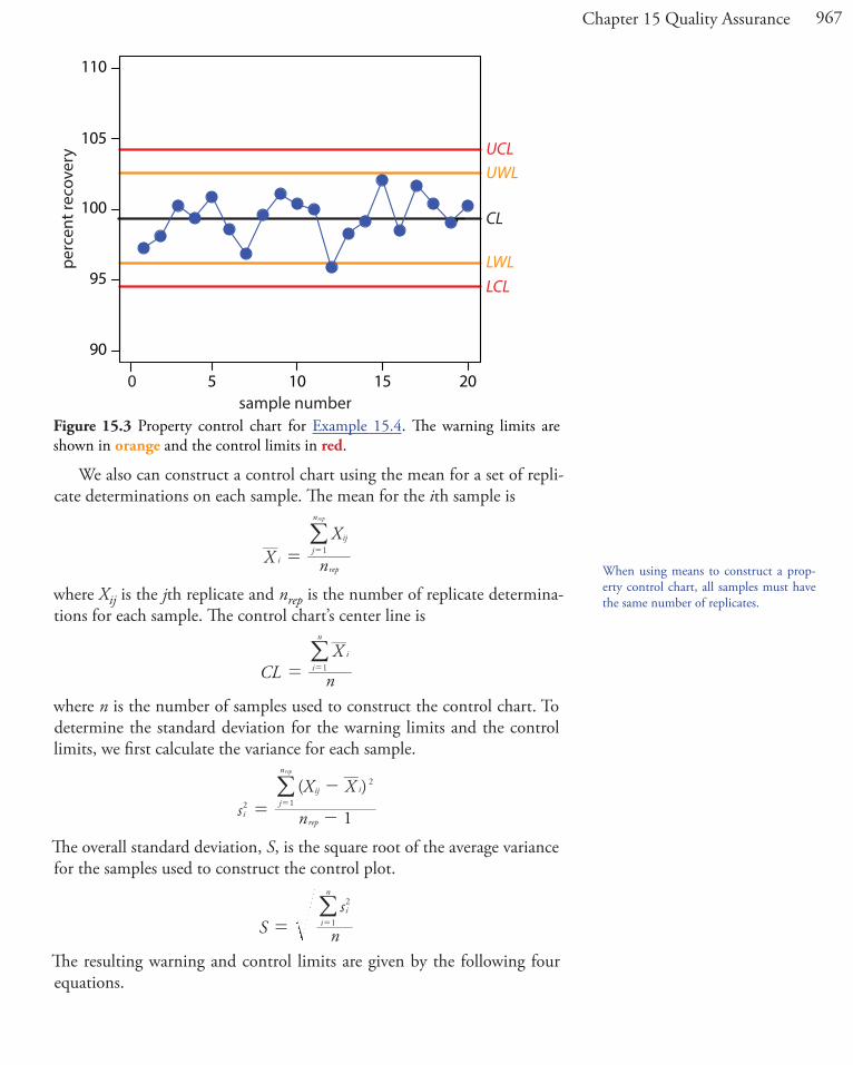
SolutionThe mean and the standard deviation for the 20 data points are 99.4% and 1.6%, respectively. Using these values, we find that the UCL is 104.2%, the UWL is 102.6%, the LWL is 96.2%, and the LCL is 94.6%. To construct the control chart, we plot the data points sequentially and draw horizontal lines for the center line and the four boundary lines. The resulting property control chart is shown in Figure 15.3.

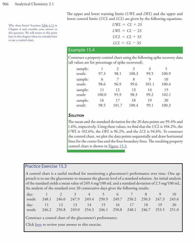
Practice Exercise 15.3A control chart is a useful method for monitoring a glucometer’s performance over time. One ap-proach is to use the glucometer to measure the glucose level of a standard solution. An initial analysis of the standard yields a mean value of 249.4 mg/100 mL and a standard deviation of 2.5 mg/100 mL. An analysis of the standard over 20 consecutive days gives the following results.day:result:

1248.1

2246.0

3247.9

4249.4

5250.9

6249.7

7250.2

8250.3

9247.3

10245.6

day:result:

11246.2

12250.8

13249.0

14254.3

15246.1

16250.8

17248.1

18246.7

19253.5

20251.0

Construct a control chart of the glucometer’s performance.


Why these limits? Examine Table 4.12 in Chapter 4 and consider your answer to this question. We will return to this point later in this chapter when we consider how to use a control chart.


Figure 15.3 Property control chart for Example 15.4. The warning limits are shown in orange and the control limits in red.

When using means to construct a prop-erty control chart, all samples must have the same number of replicates.

We also can construct a control chart using the mean for a set of repli-cate determinations on each sample. The mean for the ith sample is

X n

Xi

rep

ijj

n

1

rep

==

/

where Xij is the jth replicate and nrep is the number of replicate determina-tions for each sample. The control chart’s center line is

CL n

X ii

n

1= =

/

where n is the number of samples used to construct the control chart. To determine the standard deviation for the warning limits and the control limits, we first calculate the variance for each sample.

( )s n

X X

1irep

ij ij

n

2

2

1

rep

= -

-=

/

The overall standard deviation, S, is the square root of the average variance for the samples used to construct the control plot.

S n

sii

n2

1= =

/

The resulting warning and control limits are given by the following four equations.

5 10 15 20

90

95

100

105

110

0sample number

perc

ent r

ecov

ery

1 CL

UWL

LWL

UCL

LCL


UWL CLnS

LWL CLnS

UCL CLnS

LCL CLnS

2

2

3

3

rep

rep

rep

rep

= +

= -

= +

= -

constructing A precision control chArt

A precision control chart shows how the precision of an analysis changes over time. The most common measure of precision is the range, R, between the largest and the smallest results for nrep analyses on a sample.

R X Xlargest smallest= -

To construct the control chart, we analyze a minimum of 15–20 samples while the system is under statistical control. The center line (CL) of the control chart is the average range of these n samples.

R n

Rii

n

1= =

/

The upper warning line and the upper control line are given by the follow-ing equations

UWL f RUCL f R

UWL

UCL

#

#

=

=

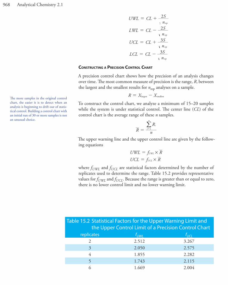
where fUWL and fUCL are statistical factors determined by the number of replicates used to determine the range. Table 15.2 provides representative values for fUWL and fUCL. Because the range is greater than or equal to zero, there is no lower control limit and no lower warning limit.

Table 15.2 Statistical Factors for the Upper Warning Limit and the Upper Control Limit of a Precision Control Chart

replicates fUWL fUCL

2 2.512 3.2673 2.050 2.5754 1.855 2.2825 1.743 2.1156 1.669 2.004

The more samples in the original control chart, the easier it is to detect when an analysis is beginning to drift our of statis-tical control. Building a control chart with an initial run of 30 or more samples is not an unusual choice.


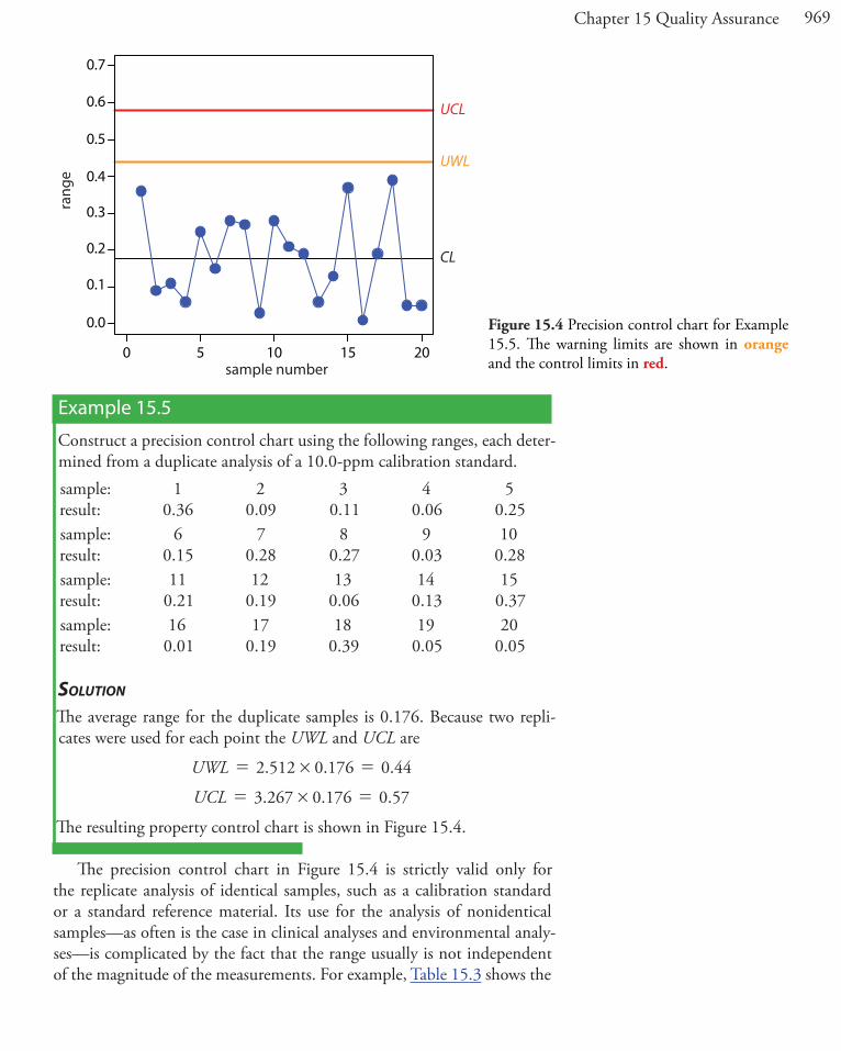
Example 15.5

Construct a precision control chart using the following ranges, each deter-mined from a duplicate analysis of a 10.0-ppm calibration standard.sample:result:

10.36

20.09

30.11

40.06

50.25

sample:result:

60.15

70.28

80.27

90.03

100.28

sample:result:

110.21

120.19

130.06

140.13

150.37

sample:result:

160.01

170.19

180.39

190.05

200.05

SolutionThe average range for the duplicate samples is 0.176. Because two repli-cates were used for each point the UWL and UCL are

. . .UWL 2 512 0 176 0 44#= =

. . .UCL 3 267 0 176 0 57#= =

The resulting property control chart is shown in Figure 15.4.

The precision control chart in Figure 15.4 is strictly valid only for the replicate analysis of identical samples, such as a calibration standard or a standard reference material. Its use for the analysis of nonidentical samples—as often is the case in clinical analyses and environmental analy-ses—is complicated by the fact that the range usually is not independent of the magnitude of the measurements. For example, Table 15.3 shows the

Figure 15.4 Precision control chart for Example 15.5. The warning limits are shown in orange and the control limits in red.

0 5 10 15 20

0.0

0.1

0.2

0.3

0.4

0.5

0.6

0.7ra

nge

sample number

UWL

UCL

CL


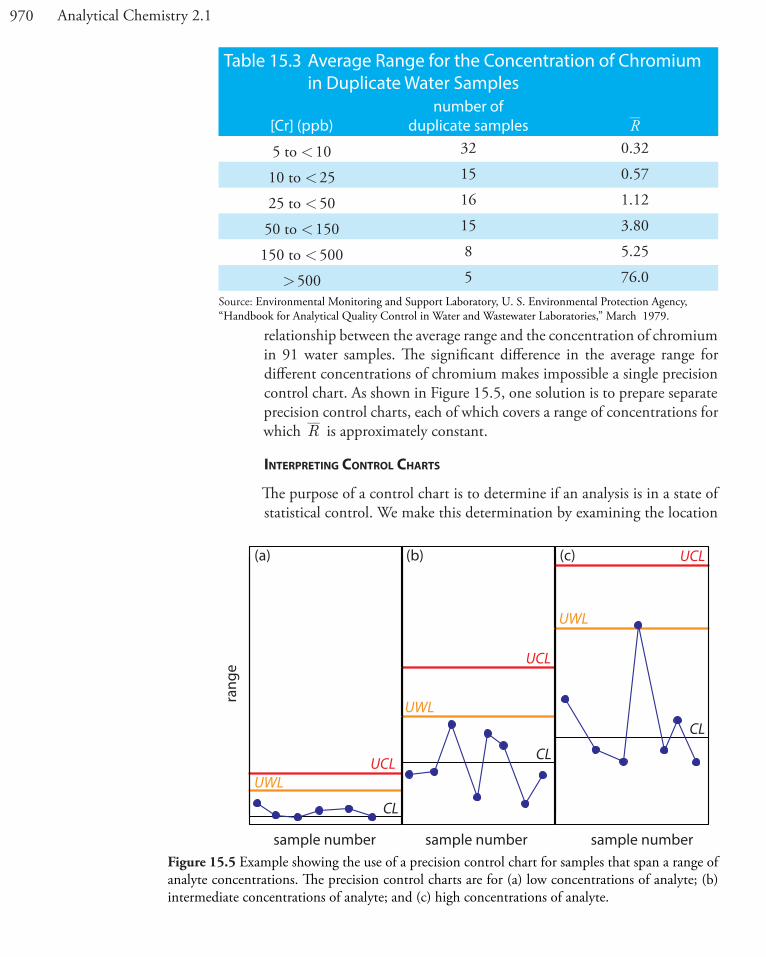
relationship between the average range and the concentration of chromium in 91 water samples. The significant difference in the average range for different concentrations of chromium makes impossible a single precision control chart. As shown in Figure 15.5, one solution is to prepare separate precision control charts, each of which covers a range of concentrations for which R is approximately constant.

interpreting control chArts

The purpose of a control chart is to determine if an analysis is in a state of statistical control. We make this determination by examining the location

rang

e

sample number sample number sample number

UWL

UWL

UWL

UCL

UCL

UCL

CL

CL

CL

(a) (b) (c)

Figure 15.5 Example showing the use of a precision control chart for samples that span a range of analyte concentrations. The precision control charts are for (a) low concentrations of analyte; (b) intermediate concentrations of analyte; and (c) high concentrations of analyte.

Table 15.3 Average Range for the Concentration of Chromium in Duplicate Water Samples

[Cr] (ppb)number of

duplicate samples R

5 to < 10 32 0.32

10 to < 25 15 0.57

25 to < 50 16 1.12

50 to < 150 15 3.80

150 to < 500 8 5.25

> 500 5 76.0Source: Environmental Monitoring and Support Laboratory, U. S. Environmental Protection Agency, “Handbook for Analytical Quality Control in Water and Wastewater Laboratories,” March 1979.


of individual results relative to the warning limits and the control limits, and by examining the distribution of results around the central line. If we assume that the individual results are normally distributed, then the proba-bility of finding a point at any distance from the control limit is determined by the properties of a normal distribution.5 We set the upper and the lower control limits for a property control chart to CL ± 3S because 99.74% of a normally distributed population falls within three standard deviations of the population’s mean. This means that there is only a 0.26% probability of obtaining a result larger than the UCL or smaller than the LCL. When a result exceeds a control limit, the most likely explanation is a systematic error in the analysis or a loss of precision. In either case, we assume that the analysis no longer is in a state of statistical control.Rule 1. An analysis is no longer under statistical control if any single

point exceeds either the UCL or the LCL.By setting the upper and lower warning limits to CL ± 2S, we expect that no more than 5% of the results will exceed one of these limits; thusRule 2. An analysis is no longer under statistical control if two out of

three consecutive points are between the UWL and the UCL or between the LWL and the LCL.

If an analysis is under statistical control, then we expect a random dis-tribution of results around the center line. The presence of an unlikely pat-tern in the data is another indication that the analysis is no longer under statistical control. Rule 3. An analysis is no longer under statistical control if seven consecu-

tive results are completely above or completely below the center line.

Rule 4. An analysis is no longer under statistical control if six consecutive results increase (or decrease) in value.

Rule 5. An analysis is no longer under statistical control if 14 consecutive results alternate up and down in value.

Rule 6. An analysis is no longer under statistical control if there is any obvious nonrandom pattern to the results.

Figure 15.6 shows three examples of control charts in which the results in-dicate that an analysis no longer is under statistical control. The same rules apply to precision control charts with the exception that there are no lower warning limits and lower control limits.

using control chArts for QuAlity AssurAnce

Control charts play an important role in a performance-based program of quality assurance because they provide an easy to interpret picture of the statistical state of an analysis. Quality assessment samples such as blanks,

5 Mullins, E. Analyst, 1994, 119, 369–375.

Figure 15.6 Examples of property control charts that show a sequence of results—indicated by the highlighting—that violate (a) rule 3; (b) rule 4; and (c) rule 5.

Practice Exercise 15.4In Practice Exercise 15.3 you cre-ated a property control chart for a glucometer. Examine your property control chart and evaluate the glu-cometer’s performance. Does your conclusion change if the next three results are 255.6, 253.9, and 255.8 mg/100 mL?


sample number

CL

UWL

LWL

UCL

LCL

resu

lt

sample number

CL

UWL

LWL

UCL

LCL

resu

lt

sample number

CL

UWL

LWL

UCL

LCL

resu

lt

(a)

(b)

(c)


standards, and spike recoveries are monitored with property control charts. A precision control chart is used to monitor duplicate samples.

The first step in using a control chart is to determine the mean value and the standard deviation (or range) for the property being measured while the analysis is under statistical control. These values are established using the same conditions that will be present during subsequent analyses. Preliminary data is collected both throughout the day and over several days to account for short-term and for long-term variability. An initial control chart is prepared using this preliminary data and discrepant points identi-fied using the rules discussed in the previous section. After eliminating questionable points, the control chart is replotted. Once the control chart is in use, the original limits are adjusted if the number of new data points is at least equivalent to the amount of data used to construct the original control chart. For example, if the original control chart includes 15 points, new limits are calculated after collecting 15 additional points. The 30 points are pooled together to calculate the new limits. A second modification is made after collecting an additional 30 points. Another indication that a control chart needs to be modified is when points rarely exceed the warning limits. In this case the new limits are recalculated using the last 20 points.

Once a control chart is in use, new quality assessment data is added at a rate sufficient to ensure that the analysis remains in statistical control. As with prescriptive approaches to quality assurance, when the analysis falls out of statistical control, all samples analyzed since the last successful verifi-cation of statistical control are reanalyzed. The advantage of a performance-based approach to quality assurance is that a laboratory may use its experi-ence, guided by control charts, to determine the frequency for collecting quality assessment samples. When the system is stable, quality assessment samples can be acquired less frequently.

15E Key Termscontrol chart duplicate samples field blankgood laboratory practices good measurement

practicesmethod blank

proficiency standard protocol for a specific purpose

quality assessment

quality assurance program quality control reagent blankspike recovery standard operations

procedurestatistical control

trip blank

15F Chapter SummaryFew analyses are so straightforward that high quality results are obtained with ease. Good analytical work requires careful planning and an attention to detail. Creating and maintaining a quality assurance program is one way


to help ensure the quality of analytical results. Quality assurance programs usually include elements of quality control and quality assessment.

Quality control encompasses all activities used to bring a system into statistical control. The most important facet of quality control is written documentation, including statements of good laboratory practices, good measurement practices, standard operating procedures, and protocols for a specific purpose.

Quality assessment includes the statistical tools used to determine whether an analysis is in a state of statistical control, and, if possible, to suggest why an analysis has drifted out of statistical control. Among the tools included in quality assessment are the analysis of duplicate samples, the analysis of blanks, the analysis of standards, and the analysis of spike recoveries.

Another important quality assessment tool, which provides an ongoing evaluation of an analysis, is a control chart. A control chart plots a property, such as a spike recovery, as a function of time. Results that exceed warning and control limits, or unusual patterns of results indicate that an analysis is no longer under statistical control.

15G Problems

1. Make a list of good laboratory practices for the lab that accompanies this course, or another lab if this course does not have an associated laboratory. Explain the rationale for each item on your list.

2. Write directives outlining good measurement practices for (a) a buret, for (b) a pH meter, and for (c) a spectrophotometer.

3. A atomic absorption method for the analysis of lead in an industrial wastewater has a method detection limit of 10 ppb. The relationship between the absorbance and the concentration of lead, as determined from a calibration curve, is

. ( )A 0 349 ppm Pb#=

Analysis of a sample in duplicate gives absorbance values of 0.554 and 0.516. Is the precision between these two duplicates acceptable based on the limits in Table 15.1?

4. The following data were obtained for the duplicate analysis of a 5.00 ppm NO3

- standard.sample X1 (ppm) X2 (ppm)

1 5.02 4.902 5.10 5.183 5.07 4.95


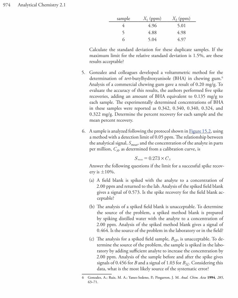
sample X1 (ppm) X2 (ppm)4 4.96 5.015 4.88 4.986 5.04 4.97

Calculate the standard deviation for these duplicate samples. If the maximum limit for the relative standard deviation is 1.5%, are these results acceptable?

5. Gonzalez and colleagues developed a voltammetric method for the determination of tert-butylhydroxyanisole (BHA) in chewing gum.6 Analysis of a commercial chewing gum gave a result of 0.20 mg/g. To evaluate the accuracy of this results, the authors performed five spike recoveries, adding an amount of BHA equivalent to 0.135 mg/g to each sample. The experimentally determined concentrations of BHA in these samples were reported as 0.342, 0.340, 0.340, 0.324, and 0.322 mg/g. Determine the percent recovery for each sample and the mean percent recovery.

6. A sample is analyzed following the protocol shown in Figure 15.2, using a method with a detection limit of 0.05 ppm. The relationship between the analytical signal, Smeas, and the concentration of the analyte in parts per million, CA, as determined from a calibration curve, is

.S C0 273meas A#=

Answer the following questions if the limit for a successful spike recov-ery is ±10%.

(a) A field blank is spiked with the analyte to a concentration of 2.00 ppm and returned to the lab. Analysis of the spiked field blank gives a signal of 0.573. Is the spike recovery for the field blank ac-ceptable?

(b) The analysis of a spiked field blank is unacceptable. To determine the source of the problem, a spiked method blank is prepared by spiking distilled water with the analyte to a concentration of 2.00 ppm. Analysis of the spiked method blank gives a signal of 0.464. Is the source of the problem in the laboratory or in the field?

(c) The analysis for a spiked field sample, BSF, is unacceptable. To de-termine the source of the problem, the sample is spiked in the labo-ratory by adding sufficient analyte to increase the concentration by 2.00 ppm. Analysis of the sample before and after the spike gives signals of 0.456 for B and a signal of 1.03 for BSL. Considering this data, what is the most likely source of the systematic error?

6 Gonzalez, A.; Ruiz, M. A.; Yanez-Sedeno, P.; Pingarron, J. M. Anal. Chim. Acta 1994, 285, 63–71.


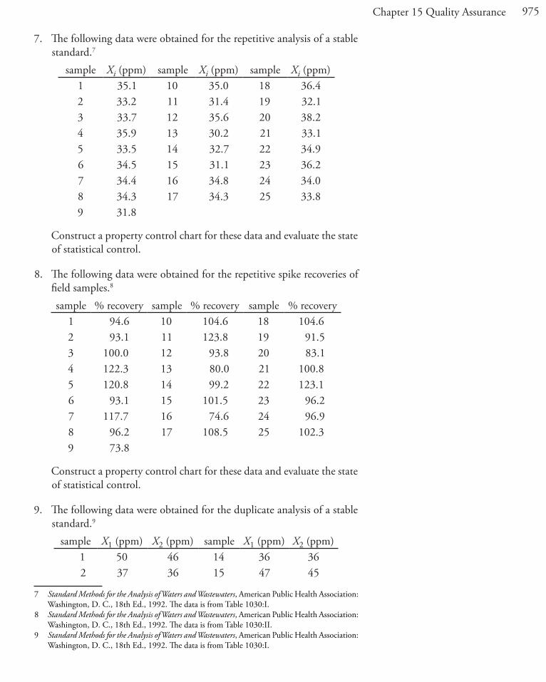
7. The following data were obtained for the repetitive analysis of a stable standard.7

sample Xi (ppm) sample Xi (ppm) sample Xi (ppm)1 35.1 10 35.0 18 36.42 33.2 11 31.4 19 32.13 33.7 12 35.6 20 38.24 35.9 13 30.2 21 33.15 33.5 14 32.7 22 34.96 34.5 15 31.1 23 36.27 34.4 16 34.8 24 34.08 34.3 17 34.3 25 33.89 31.8

Construct a property control chart for these data and evaluate the state of statistical control.

8. The following data were obtained for the repetitive spike recoveries of field samples.8

sample % recovery sample % recovery sample % recovery1 94.6 10 104.6 18 104.62 93.1 11 123.8 19 91.53 100.0 12 93.8 20 83.14 122.3 13 80.0 21 100.85 120.8 14 99.2 22 123.16 93.1 15 101.5 23 96.27 117.7 16 74.6 24 96.98 96.2 17 108.5 25 102.39 73.8

Construct a property control chart for these data and evaluate the state of statistical control.

9. The following data were obtained for the duplicate analysis of a stable standard.9

sample X1 (ppm) X2 (ppm) sample X1 (ppm) X2 (ppm)1 50 46 14 36 362 37 36 15 47 45

7 Standard Methods for the Analysis of Waters and Wastewaters, American Public Health Association: Washington, D. C., 18th Ed., 1992. The data is from Table 1030:I.

8 Standard Methods for the Analysis of Waters and Wastewaters, American Public Health Association: Washington, D. C., 18th Ed., 1992. The data is from Table 1030:II.

9 Standard Methods for the Analysis of Waters and Wastewaters, American Public Health Association: Washington, D. C., 18th Ed., 1992. The data is from Table 1030:I.


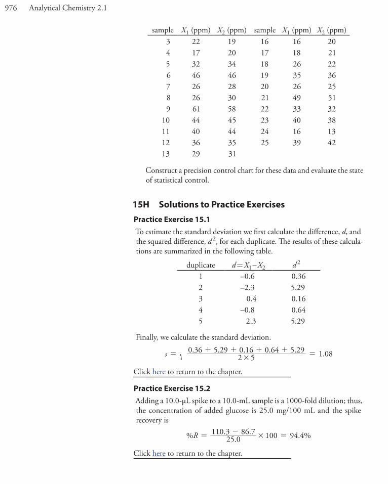
sample X1 (ppm) X2 (ppm) sample X1 (ppm) X2 (ppm)3 22 19 16 16 204 17 20 17 18 215 32 34 18 26 226 46 46 19 35 367 26 28 20 26 258 26 30 21 49 519 61 58 22 33 32

10 44 45 23 40 3811 40 44 24 16 1312 36 35 25 39 4213 29 31

Construct a precision control chart for these data and evaluate the state of statistical control.

15H Solutions to Practice ExercisesPractice Exercise 15.1To estimate the standard deviation we first calculate the difference, d, and the squared difference, d 2, for each duplicate. The results of these calcula-tions are summarized in the following table.

duplicate d = X1 – X2 d 2

1 –0.6 0.362 –2.3 5.293 0.4 0.164 –0.8 0.645 2.3 5.29

Finally, we calculate the standard deviation.. . . . . .s 2 5

0 36 5 29 0 16 0 64 5 29 1 08#= + + + + =

Click here to return to the chapter.

Practice Exercise 15.2Adding a 10.0-µL spike to a 10.0-mL sample is a 1000-fold dilution; thus, the concentration of added glucose is 25.0 mg/100 mL and the spike recovery is

% .. . . %R 25 0

110 3 86 7 100 94 4#= - =



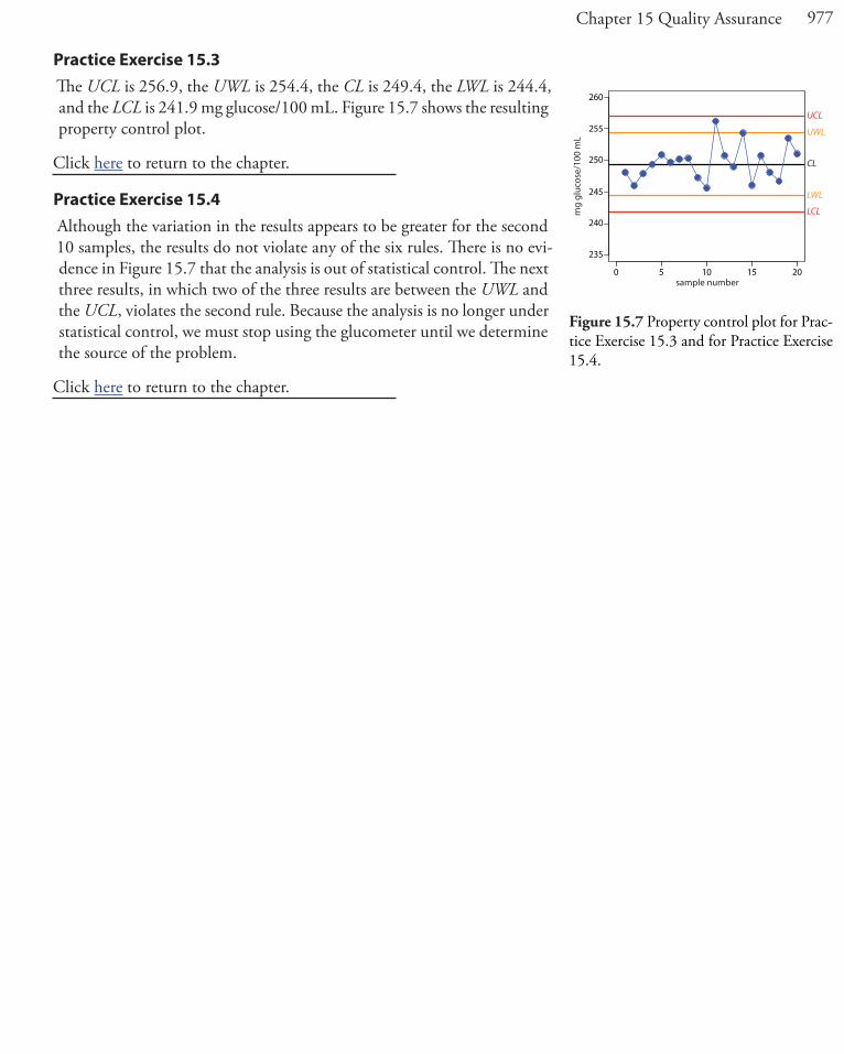
Practice Exercise 15.3The UCL is 256.9, the UWL is 254.4, the CL is 249.4, the LWL is 244.4, and the LCL is 241.9 mg glucose/100 mL. Figure 15.7 shows the resulting property control plot.


Practice Exercise 15.4Although the variation in the results appears to be greater for the second 10 samples, the results do not violate any of the six rules. There is no evi-dence in Figure 15.7 that the analysis is out of statistical control. The next three results, in which two of the three results are between the UWL and the UCL, violates the second rule. Because the analysis is no longer under statistical control, we must stop using the glucometer until we determine the source of the problem.


Figure 15.7 Property control plot for Prac-tice Exercise 15.3 and for Practice Exercise 15.4.

0 5 10 15 20

235

240

245

250

255

260

sample number

mg

gluc

ose/

100

mL

UCL

UWL

CL

LWL

LCL

chapter 15dpuadweb.depauw.edu/harvey_web/etextproject/ac2.1files/chapter15.pdf954 analytical...

Documents