chapter 2. ways forward for...
TRANSCRIPT
21
CHAPTER 2. WAYS FORWARD FOR CLIMATOLOGY
2.1 Although mostly arid or semi-arid, the Arab region encompasses a diversity of climates,
including temperate zones in the northern and higher elevations of the Maghreb and Mashreq,
tropical ocean climates in the Comoros, and varied coastal climates fronting the Mediterranean, Red
and Arabian Seas, the Gulf of Arabia and the Indian Ocean (Figures 2.3 and 2.4). Climate change is
expected to have different impacts in these different climate zones.
2.2 To date, the Arab region has not been addressed as a discrete region in climate change
research assessments, such as in the IPCC reports. Typically, information must be inferred from
analyses carried out in other regions. Recent literature from regional studies confirms the broad
conclusions of the IPCC Fourth Assessment Report (AR4) regarding increasing temperatures and
mostly reduced precipitation, but sometimes differs quite substantially regarding the details. This
problem is particularly severe for the Arabian Peninsula, where models disagree about whether
there will be more or less precipitation. The future climate in this region will depend in large part on
the position of the Inter-Tropical Convergence Zone (ITCZ) (see Box 2.1); all models project that it
will move further northward, but disagree on the precise amount and location of that shift. Much of
the region also falls in the transitional zone between areas with projected decreases in rainfall and
those with projected increases. Since models differ as to the precise location of that transition, it is
often difficult to project the exact magnitude of precipitation changes or even whether there will be
more or less rainfall.
2.3 While several efforts are underway to improve on the availability of downscaled climate
change information for the Arab region based on existing global and regional circulation models
and scenarios, the international climate change modeling community is moving ahead with new
global modeling approaches and climate change scenarios. This effort will include a new set of
improved and consistent modeling results that will be available for all regions, with the first results
appearing within the next one to two years.
2.4 Climate projections depend on having a good set of observational data to determine
current trends and to translate outputs from global circulation models to regional scales
(downscaling). Unfortunately, many observational and modeling gaps exist in the study of climate
change in the Arab region. In these circumstances, it is important not to fall into the trap of
extrapolating from global information and applying it to the region, or of jumping from
interpretations of long-term projections to statements about the near term. This chapter brings
together the various pieces of work that have been done for the Arab region, which provide an
insight into the region‘s future climate. The Arab region will remain predominately arid with some
areas becoming even drier and hotter, but rainfall patterns will change and the increase in flooding
events already being observed is likely to continue in the future.
22
Box 2.1 Some Basic Definitions22
Climate: Climate, in a narrow sense, is usually defined as the average of weather, or more rigorously, as the
statistical description in terms of the mean and variability of relevant quantities over a period of time ranging
from months to thousands or millions of years. The classical period for averaging these variables is 30 years,
as defined by the World Meteorological Organization. The relevant variables are most often surface
parameters, such as temperature, precipitation and wind. Climate, in a wider sense, is the state, including a
statistical description, of the climate system.
Climate change: Climate change refers to a long-term change in the state of the climate that can be
identified (e.g., by using statistical tests) by changes in the mean and/or the variability of its properties, and
that persists for an extended period, typically decades or longer. Climate change may be due to natural
internal processes or external forcings, or to persistent anthropogenic changes in the composition of the
atmosphere or in land use. Note that Article 1 of the UN Framework Convention on Climate Change
(UNFCCC) defines climate change as: ―a change of climate which is attributed directly or indirectly to
human activity that alters the composition of the global atmosphere and which is in addition to natural
climate variability observed over comparable time periods.‖ The UNFCCC thus makes a distinction between
climate change attributable to human activities altering the atmospheric composition, and climate variability
attributable to natural causes.
Climate scenario: A plausible and often simplified representation of the future climate, based on an
internally consistent set of climatological relationships that has been constructed for explicit use in
investigating the potential consequences of anthropogenic climate change, often serving as input to impact
models. Climate projections often serve as the raw material for constructing climate scenarios, but climate
scenarios usually require additional information, such as information about the observed current climate. A
climate change scenario is the difference between a climate scenario and the current climate.
Climate variability: Climate variability refers to variations in the mean state and other statistics (such as
standard deviations, the occurrence of extremes, etc.) of the climate on all spatial and temporal scales beyond
that of individual weather events. Variability may be due to natural internal processes within the climate
system (internal variability), or to variations in natural or anthropogenic external forcing (external
variability).
North Atlantic Oscillation (NAO): The North Atlantic Oscillation consists of opposing variations of
barometric pressure between areas near Iceland and near the Azores. It affects the strength and position of
the main westerly winds across the Atlantic into Europe and the Mediterranean. When the pressure
difference is high (NAO+), the westerlies are stronger and track more to the north leading to cool summers
and mild wet winters in Europe, but drier conditions in the Mediterranean. In the opposite phase, the
westerlies and the storms they bring track further south leading to cold winters in Europe, but more storms in
the Mediterranean and more rain in North Africa.
Inter-Tropical Convergence Zone (ITCZ) The Inter-Tropical Convergence Zone is an equatorial zonal belt
of low pressure near the equator where the northeast trade winds meet the southeast trade winds. As these
winds converge, moist air is forced upward, resulting in a band of heavy precipitation. This band moves
seasonally. In Africa, it reaches its northernmost position in summer and also interacts with the Indian
Monsoon, bringing rains to the southern part of the Arab Region (Southern Sahel), but the northward extent
varies from year to year making both conventional weather forecasting and climate modeling difficult.
Storm surge: Storm surge is a rise of the sea water above the normal level along a shore associated with a
low pressure weather system, typically tropical cyclones and strong extratropical cyclones. It is the result of
both the low pressure at the center of the storm raising the ocean surface, as well as the wind pushing the
22Largely these definitions are based on those provided within AR4.
23
water in the direction the storm is moving. The storm surge is responsible for most loss of life in tropical
cyclones worldwide.
Flash floods: Flash floods usually refer to rapid flooding that happens very suddenly, usually without
advance warning. They are different from regular floods, as they often last less than six hours. Flash floods,
with intense rainfall normally occur in association with the passage of a storm or tropical cyclone, especially
when the rain falls too quickly on saturated soil or dry soil that has poor absorption capacity. Flash floods
may also refer to a flooding situation, when barriers holding back water fail, such as the collapse of a natural
ice or debris dam, or a man-made dam.
Tropical cyclone: A storm system characterized by a large low-pressure center and numerous thunderstorms
that produce strong winds and heavy rain. Tropical cyclones strengthen when water evaporated from the
ocean is released as the saturated air rises, resulting in condensation of water vapor contained in the moist
air. They are fuelled by a different heat mechanism than other cyclonic windstorms such as nor'easters and
European windstorms. The characteristic that separates tropical cyclones from other cyclonic systems is that
at any height in the atmosphere, the center of a tropical cyclone will be warmer than its surrounds; a
phenomenon called ―warm core‖ storm systems. The term ―tropical‖ refers to both the geographic origin of
these systems, which form almost exclusively in tropical regions of the globe, and their formation in
maritime tropical air masses.
Heat wave: A prolonged period of excessively hot weather, which may be accompanied by high humidity.
There is no universal definition of a heat wave; the term is relative to the usual weather in the area.
Temperatures that people from a hotter climate consider normal can be termed a heat wave in a cooler area if
they are outside the normal climate pattern for that area. The term is applied both to routine weather
variations and to extraordinary spells of heat, which may occur only once a century. Severe heat waves have
caused catastrophic crop failures, thousands of deaths from hyperthermia and other severe damages.
DESPITE SPARSE OBSERVATIONAL DATA IT IS CLEAR THAT MOST OF THE ARAB
REGION IS BECOMING HOTTER AND DRIER
2.5 The climate in Arab countries ranges from Mediterranean, with warm and dry summers
and some wintertime precipitation, through subtropical zones, with variable amounts of summer
monsoon rains, to deserts with virtually no rain. During winter, variability in the North Atlantic
Oscillation (NAO) (see Box 2.1) influences the position of storm tracks, and annual variations in
precipitation in western and central North Africa (the Maghreb) are largely governed by this NAO
effect. The eastern part of the region (most of the Mashreq, Gulf and Center Regions), where it rains
mainly during the summer, is influenced by the Indian monsoon system, which is largely controlled
by the position of the ITCZ (see Box 2.1).
There is a scarcity of meteorological surface observation
2.6 With a few exceptions, the availability of climate-station data to establish baseline
climate across the Arab region is very limited compared to most other parts of the world (Figures
2.1 and 2.2). This hampers detection of climate change, as well as the interpretation of projected
changes, since changes must be compared to a verifiable current climate. The rescue of existing but
undigitized climate data and the establishment of well-chosen, permanent, high-quality
observational sites will be necessary to establish more rigorous models in the future.
2.7 The distribution of quality-controlled, long-term observational sites within the Arab
region is uneven. For historical reasons, a reasonable number of stations exist along the Nile and the
coast of the Mediterranean Sea, but in the desert regions, coverage is very sparse. Few data are
24
available for countries, such as Libya, Gaza and the West Bank, Saudi Arabia and Somalia. For
Algeria, Tunisia, Egypt, Iraq, Sudan and the Comoros, data is probably available, but not readily
accessible. Conflict in parts of the region disrupts both the collection and sharing of data. However,
it is likely that in many areas, additional data are being gathered by various agencies, but not
entered into more widely available meteorological databases. For example, research in Yemen
quickly identified a large number of additional meteorological observation sites held only by the
Ministry of Irrigation and Agriculture (Figure 2.2b, Wilby pers. comm., 2011).
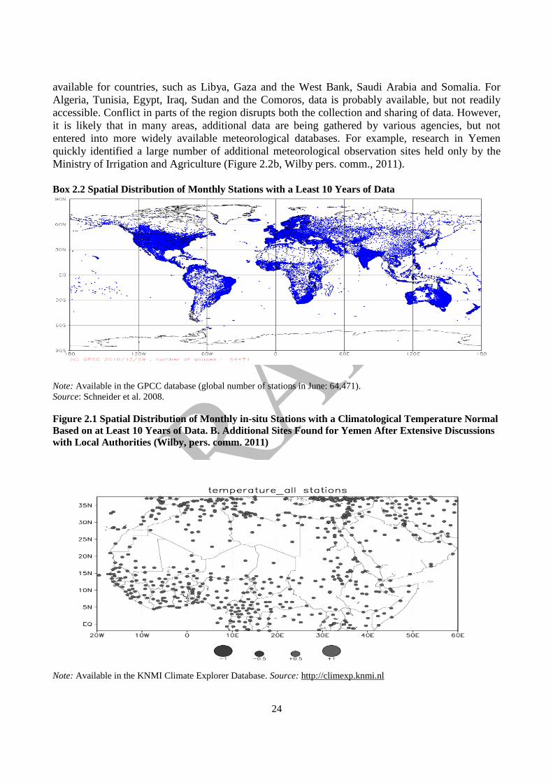
Box 2.2 Spatial Distribution of Monthly Stations with a Least 10 Years of Data
Note: Available in the GPCC database (global number of stations in June: 64,471).
Source: Schneider et al. 2008.
Figure 2.1 Spatial Distribution of Monthly in-situ Stations with a Climatological Temperature Normal
Based on at Least 10 Years of Data. B. Additional Sites Found for Yemen After Extensive Discussions
with Local Authorities (Wilby, pers. comm. 2011)
Note: Available in the KNMI Climate Explorer Database. Source: http://climexp.knmi.nl
25
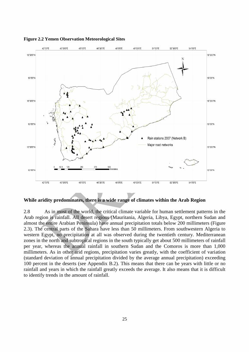
Figure 2.2 Yemen Observation Meteorological Sites
While aridity predominates, there is a wide range of climates within the Arab Region
2.8 As in most of the world, the critical climate variable for human settlement patterns in the
Arab region is rainfall. All desert regions (Mauritania, Algeria, Libya, Egypt, northern Sudan and
almost the entire Arabian Peninsula) have annual precipitation totals below 200 millimeters (Figure
2.3). The central parts of the Sahara have less than 50 millimeters. From southwestern Algeria to
western Egypt, no precipitation at all was observed during the twentieth century. Mediterranean
zones in the north and subtropical regions in the south typically get about 500 millimeters of rainfall
per year, whereas the annual rainfall in southern Sudan and the Comoros is more than 1,000
millimeters. As in other arid regions, precipitation varies greatly, with the coefficient of variation
(standard deviation of annual precipitation divided by the average annual precipitation) exceeding
100 percent in the deserts (see Appendix B.2). This means that there can be years with little or no
rainfall and years in which the rainfall greatly exceeds the average. It also means that it is difficult
to identify trends in the amount of rainfall.
26
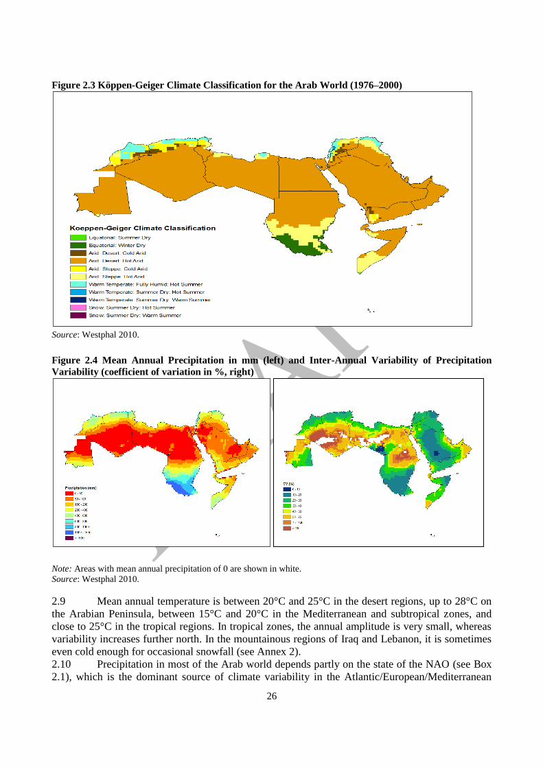
Figure 2.3 Köppen-Geiger Climate Classification for the Arab World (1976–2000)
Source: Westphal 2010.
Figure 2.4 Mean Annual Precipitation in mm (left) and Inter-Annual Variability of Precipitation
Variability (coefficient of variation in %, right)
Note: Areas with mean annual precipitation of 0 are shown in white.
Source: Westphal 2010.
2.9 Mean annual temperature is between 20°C and 25°C in the desert regions, up to 28°C on
the Arabian Peninsula, between 15°C and 20°C in the Mediterranean and subtropical zones, and
close to 25°C in the tropical regions. In tropical zones, the annual amplitude is very small, whereas
variability increases further north. In the mountainous regions of Iraq and Lebanon, it is sometimes
even cold enough for occasional snowfall (see Annex 2).
2.10 Precipitation in most of the Arab world depends partly on the state of the NAO (see Box
2.1), which is the dominant source of climate variability in the Atlantic/European/Mediterranean
27
region. Its influence can be seen in weather patterns, streamflows and subsequent ecological and
agricultural effects. Cullen et al. (2002) identified two components of Middle Eastern streamflow
variability. The first principal component reflects rainfall-driven runoff and explains 80 percent of
the variability in river flows from December to March. This principal component is correlated, on
interannual to interdecadal timescales, to the NAO phase (in a positive NAO phase, the climate in
the Middle East is cooler and drier than average and vice versa when NAO is in a negative phase).
The second principal component (the so-called Khamsin) is related to spring snow melt in the
mountains and explains more than half of the streamflow variability from April to June. A
prevailing positive NAO phase, as in the 1990s and 2000s, can therefore result in drought
conditions in the region, including in the Euphrates-Tigris and Jordan Rivers Basins.
Arab countries have warmed and most have become drier
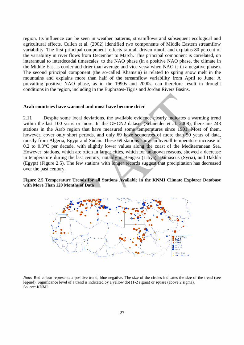
2.11 Despite some local deviations, the available evidence clearly indicates a warming trend
within the last 100 years or more. In the GHCN2 dataset (Schneider et al. 2008), there are 243
stations in the Arab region that have measured some temperatures since 1901. Most of them,
however, cover only short periods, and only 69 have sequences of more than 50 years of data,
mostly from Algeria, Egypt and Sudan. These 69 stations show an overall temperature increase of
0.2 to 0.3°C per decade, with slightly lower values along the coast of the Mediterranean Sea.
However, stations, which are often in larger cities, which for unknown reasons, showed a decrease
in temperature during the last century, notably in Bengasi (Libya), Damascus (Syria), and Dakhla
(Egypt) (Figure 2.5). The few stations with longer records suggest that precipitation has decreased
over the past century.
Figure 2.5 Temperature Trends for all Stations Available in the KNMI Climate Explorer Database
with More Than 120 Months of Data
Note: Red colour represents a positive trend, blue negative. The size of the circles indicates the size of the trend (see
legend). Significance level of a trend is indicated by a yellow dot (1-2 sigma) or square (above 2 sigma).
Source: KNMI.
28
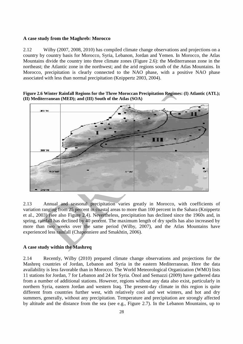
A case study from the Maghreb: Morocco
2.12 Wilby (2007, 2008, 2010) has compiled climate change observations and projections on a
country by country basis for Morocco, Syria, Lebanon, Jordan and Yemen. In Morocco, the Atlas
Mountains divide the country into three climate zones (Figure 2.6): the Mediterranean zone in the
northeast; the Atlantic zone in the northwest; and the arid regions south of the Atlas Mountains. In
Morocco, precipitation is clearly connected to the NAO phase, with a positive NAO phase
associated with less than normal precipitation (Knippertz 2003, 2004).
Figure 2.6 Winter Rainfall Regions for the Three Moroccan Precipitation Regimes: (I) Atlantic (ATL);
(II) Mediterranean (MED); and (III) South of the Atlas (SOA)
2.13 Annual and seasonal precipitation varies greatly in Morocco, with coefficients of
variation ranging from 25 percent in coastal areas to more than 100 percent in the Sahara (Knippertz
et al., 2003) (see also Figure 2.4). Nevertheless, precipitation has declined since the 1960s and, in
spring, rainfall has declined by 40 percent. The maximum length of dry spells has also increased by
more than two weeks over the same period (Wilby, 2007), and the Atlas Mountains have
experienced less rainfall (Chaponniere and Smakhtin, 2006).
A case study within the Mashreq
2.14 Recently, Wilby (2010) prepared climate change observations and projections for the
Mashreq countries of Jordan, Lebanon and Syria in the eastern Mediterranean. Here the data
availability is less favorable than in Morocco. The World Meteorological Organization (WMO) lists
11 stations for Jordan, 7 for Lebanon and 24 for Syria. Önol and Semazzi (2009) have gathered data
from a number of additional stations. However, regions without any data also exist, particularly in
northern Syria, eastern Jordan and western Iraq. The present-day climate in this region is quite
different from countries further west, with relatively cool and wet winters, and hot and dry
summers, generally, without any precipitation. Temperature and precipitation are strongly affected
by altitude and the distance from the sea (see e.g., Figure 2.7). In the Lebanon Mountains, up to
29
1400 millimeters/year of precipitation are observed (in winter often as snow), but the deserts of
southeast Syria and southern Jordan receive less than 100 millimeters/year. Temperatures above
50°C have been observed near the Dead Sea. To explore the time-space characteristics of
precipitation, daily rescaled data from the TRMM satellite observations (Kummerowet al., 2000;
Simpson et al., 1988) have been used.
2.15 A temperature rise since the 1970s has been observed in all three countries. Mahwed
(2008) considers meteorological records at 26 stations in Syria; Freiwan and Kadioglu (2008a,
2008b) examined monthly precipitation data from Jordan; and Shahin (2007) has looked at several
stations throughout the Middle East. The greatest warming has occurred for summer minimum
temperatures, which have risen at a rate of 0.4°C/decade. Consequently, a decrease in the diurnal
temperature range has been observed, which is consistent with earlier studies (Nasrallah and
Balling, 1993; Zhang et al., 2005). There is no clear indication whether precipitation has changed in
recent decades, but estimates from TRMM data (Figure 2.7) suggest a slight decrease in winter and
spring, probably related to shifts in cyclone tracks. However, the trends are small compared to the
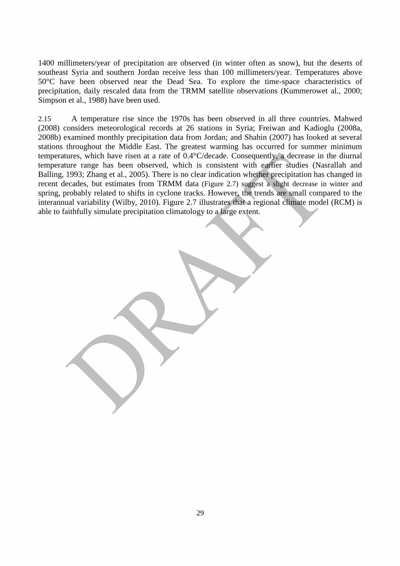
interannual variability (Wilby, 2010). Figure 2.7 illustrates that a regional climate model (RCM) is
able to faithfully simulate precipitation climatology to a large extent.
30
Figure 2.7 Spatial Distribution of Rainfall; observed in right column and simulated by NNRP2-
RegCM (left) all Averaged Over the Period 1998–2009
Note: Rainfall (millimeters) obtained from the TRMM data averaged over 1998–2009 is shown in the right panels (b, d
and f).
Source: Almazroui (2011).
A case study from the Arabian Peninsula
2.16 Wilby (2008) also compiled an assessment of climate and climate change for Yemen,
despite the lack of reliable data. Obvious errors (Wilby, 2008) and missing data make it particularly
31
difficult to apply statistical downscaling procedures. In addition, a lack of obvious trends in rainfall
averages or extremes may be, in part, due to bad data. The only station in Yemen with a reasonably
long and reliable time series for precipitation is Aden, for which monthly means exist since 1880.
However, this station shows no significant trends in annual precipitation.
More extreme events are being observed
2.17 From a climate change point of view, changes in extremes are more interesting than
changes in average values. Unfortunately, researchers do not always use the same definitions of
extremes (Bonsal et al., 2001), making it difficult to make global or even regional comparisons.
Frich et al. (2002) tried to standardize definitions of extreme indices, but they focused on areas with
ample data, which meant they were difficult to apply in large parts of the world, including the Arab
region. To address these issues and to provide better input to the IPCC AR4, a WMO expert team
defined a number of indices recommended for use in all analyses of extremes. Numerous regional
workshops were held, one of them covering the Middle East (Sensoy et al., 2005), to collect and
analyze (including quality control and homogeneity testing) data for a region from Turkey to Iran
and from Georgia to the southern tip of the Arabian Peninsula, thus covering most of the eastern
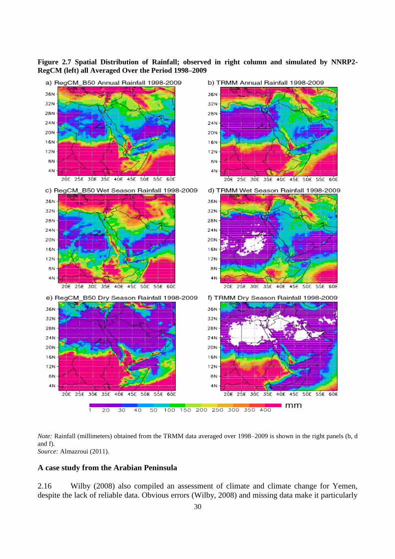
part of the region of interest in this assessment. Fifty-two stations from 15 countries that passed all
quality checks were chosen (mapped in Figure 2.8 and listed in Table 2.1).
Figure 2.8 Location of Mideast Stations for which Extreme Climate Trends Have Been Calculated
Source: Zhang et al. (2005).
32
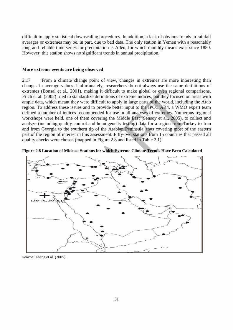
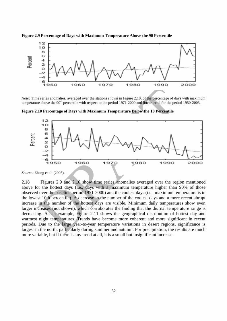
Figure 2.9 Percentage of Days with Maximum Temperature Above the 90 Percentile
Note: Time series anomalies, averaged over the stations shown in Figure 2.10, of the percentage of days with maximum
temperature above the 90th
percentile with respect to the period 1971-2000 and linear trend for the period 1950-2003.
Figure 2.10 Percentage of Days with Maximum Temperature Below the 10 Percentile
Source: Zhang et al. (2005).
2.18 Figures 2.9 and 2.10 show time series anomalies averaged over the region mentioned
above for the hottest days (i.e., days with a maximum temperature higher than 90% of those
observed over the baseline period 1971-2000) and the coolest days (i.e., maximum temperature is in
the lowest 10th percentile). A decrease in the number of the coolest days and a more recent abrupt
increase in the number of the hottest days are visible. Minimum daily temperatures show even
larger increases (not shown), which corroborates the finding that the diurnal temperature range is
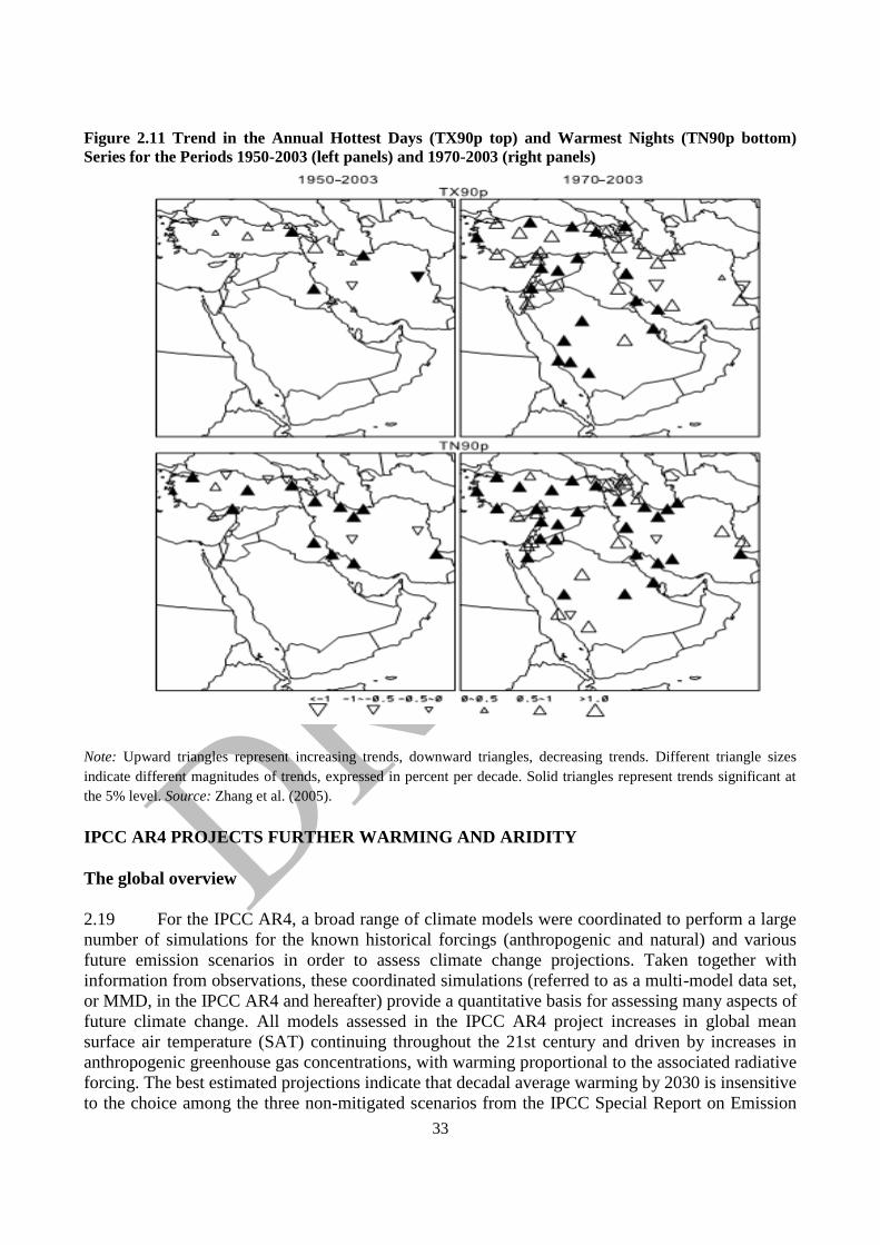
decreasing. As an example, Figure 2.11 shows the geographical distribution of hottest day and
warmest night temperatures. Trends have become more coherent and more significant in recent
periods. Due to the large year-to-year temperature variations in desert regions, significance is
largest in the north, particularly during summer and autumn. For precipitation, the results are much
more variable, but if there is any trend at all, it is a small but insignificant increase.
33
Figure 2.11 Trend in the Annual Hottest Days (TX90p top) and Warmest Nights (TN90p bottom)
Series for the Periods 1950-2003 (left panels) and 1970-2003 (right panels)
Note: Upward triangles represent increasing trends, downward triangles, decreasing trends. Different triangle sizes
indicate different magnitudes of trends, expressed in percent per decade. Solid triangles represent trends significant at
the 5% level. Source: Zhang et al. (2005).
IPCC AR4 PROJECTS FURTHER WARMING AND ARIDITY
The global overview
2.19 For the IPCC AR4, a broad range of climate models were coordinated to perform a large
number of simulations for the known historical forcings (anthropogenic and natural) and various
future emission scenarios in order to assess climate change projections. Taken together with
information from observations, these coordinated simulations (referred to as a multi-model data set,
or MMD, in the IPCC AR4 and hereafter) provide a quantitative basis for assessing many aspects of
future climate change. All models assessed in the IPCC AR4 project increases in global mean
surface air temperature (SAT) continuing throughout the 21st century and driven by increases in
anthropogenic greenhouse gas concentrations, with warming proportional to the associated radiative
forcing. The best estimated projections indicate that decadal average warming by 2030 is insensitive
to the choice among the three non-mitigated scenarios from the IPCC Special Report on Emission
34
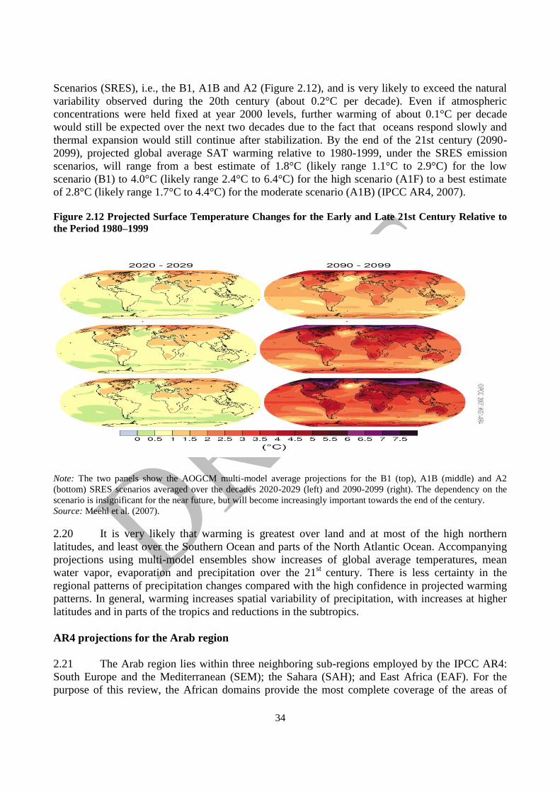
Scenarios (SRES), i.e., the B1, A1B and A2 (Figure 2.12), and is very likely to exceed the natural
variability observed during the 20th century (about 0.2°C per decade). Even if atmospheric
concentrations were held fixed at year 2000 levels, further warming of about 0.1°C per decade
would still be expected over the next two decades due to the fact that oceans respond slowly and
thermal expansion would still continue after stabilization. By the end of the 21st century (2090-
2099), projected global average SAT warming relative to 1980-1999, under the SRES emission
scenarios, will range from a best estimate of 1.8°C (likely range 1.1°C to 2.9°C) for the low
scenario (B1) to 4.0°C (likely range 2.4°C to 6.4°C) for the high scenario (A1F) to a best estimate
of 2.8°C (likely range 1.7°C to 4.4°C) for the moderate scenario (A1B) (IPCC AR4, 2007).
Figure 2.12 Projected Surface Temperature Changes for the Early and Late 21st Century Relative to
the Period 1980–1999
Note: The two panels show the AOGCM multi-model average projections for the B1 (top), A1B (middle) and A2
(bottom) SRES scenarios averaged over the decades 2020-2029 (left) and 2090-2099 (right). The dependency on the
scenario is insignificant for the near future, but will become increasingly important towards the end of the century.
Source: Meehl et al. (2007).
2.20 It is very likely that warming is greatest over land and at most of the high northern
latitudes, and least over the Southern Ocean and parts of the North Atlantic Ocean. Accompanying
projections using multi-model ensembles show increases of global average temperatures, mean
water vapor, evaporation and precipitation over the 21st
century. There is less certainty in the
regional patterns of precipitation changes compared with the high confidence in projected warming
patterns. In general, warming increases spatial variability of precipitation, with increases at higher
latitudes and in parts of the tropics and reductions in the subtropics.
AR4 projections for the Arab region
2.21 The Arab region lies within three neighboring sub-regions employed by the IPCC AR4:
South Europe and the Mediterranean (SEM); the Sahara (SAH); and East Africa (EAF). For the
purpose of this review, the African domains provide the most complete coverage of the areas of
Figure SPM.6

35
interest. Projected changes in climate are thus taken from global climate model (GCM) results for
the SAH and EAF sub-regions and the African domain (Figures 2.13 and 2.14).
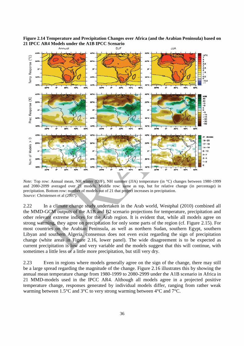
Both the SAH and EAF regions are expected to warm by between 3°C and 4°C by the late 21st
Century under the SRES A1B emission scenario, which is roughly 1.5 times the global mean
response. Warming is evident in all seasons, with the greatest increase in summer (Figures 2.13
and 2.14, upper panel) (Christensen et al., 2007).
Annual rainfall is expected to decrease in much of Mediterranean Africa and the northern
Sahara, but increase in East Africa and the southern half of the Arabian Peninsula. A 20 percent
drying in the annual mean is typical along the African Mediterranean coast in the A1B scenario
by the late 21st century in nearly every MMD model, with drying extended into the northern
Sahara and down the west coast. The annual number of precipitation days is very likely to
decrease, and the risk of summer drought is likely to increase in the Mediterranean basin.
However, mainly due to a spread in the projected northward displacement of the ITCZ, there is
no consensus amongst the 21 MMD-GCMs about the projected precipitation changes over most
of the Arabian Peninsula and over the Sahel region. (Figure 2.16, middle and lower panels;
Christensen et al., 2007). Since these regions are mostly very dry, the implication is that little
change is expected, but a substantial increase in precipitation during the summer is possible if
the ITCZ moves further northwards as some models suggest it will.
Figure 2.13 Temperature Anomalies with Respect to the Period 1901 to 1950
Note: Temperature anomalies with respect to 1901 to 1950 for two ‗African‘ land regions (SAH, left, and EAF, right)
for 1906 to 2005 (black line) and as simulated (red envelope) by the IPCC AR4 models incorporating known forcings;
and as projected for 2001 to 2100 for the A1B scenario (orange envelope). The bars at the end of the orange envelope
represent the range of projected changes for 2091 to 2100 for the B1 scenario (blue), the A1B scenario (orange) and the
A2 scenario (red). The black line is dashed where observations are present for less than 50% of the area in the decade
concerned.
Source: Christensen et al. (2007).
36
Figure 2.14 Temperature and Precipitation Changes over Africa (and the Arabian Peninsula) based on
21 IPCC AR4 Models under the A1B IPCC Scenario
Note: Top row: Annual mean, NH winter (DJF), NH summer (JJA) temperature (in °C) changes between 1980-1999
and 2080-2099 averaged over 21 models. Middle row: same as top, but for relative change (in percentage) in
precipitation. Bottom row: number of models out of 21 that project increases in precipitation. Source: Christensen et al (2007).
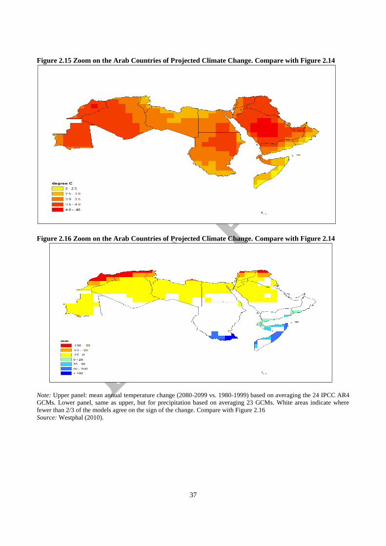
2.22 In a climate change study undertaken in the Arab world, Westphal (2010) combined all
the MMD-GCM outputs of the A1B and B2 scenario projections for temperature, precipitation and
other relevant extreme indices for the Arab region. It is evident that, while all models agree on
strong warming, they agree on precipitation for only some parts of the region (cf. Figure 2.15). For
most countries on the Arabian Peninsula, as well as northern Sudan, southern Egypt, southern
Libyan and southern Algeria, consensus does not even exist regarding the sign of precipitation
change (white areas in Figure 2.16, lower panel). The wide disagreement is to be expected as
current precipitation is low and very variable and the models suggest that this will continue, with
sometimes a little less or a little more precipitation, but still very dry.
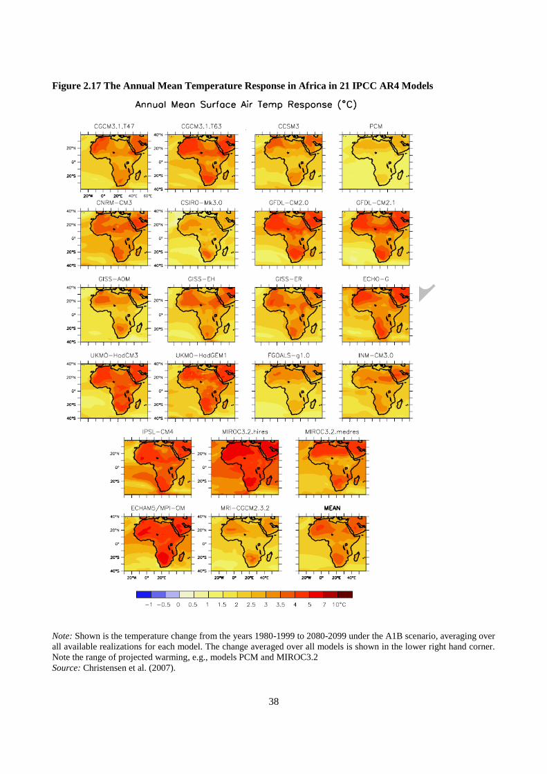
2.23 Even in regions where models generally agree on the sign of the change, there may still
be a large spread regarding the magnitude of the change. Figure 2.16 illustrates this by showing the
annual mean temperature change from 1980-1999 to 2080-2999 under the A1B scenario in Africa in
21 MMD-models used in the IPCC AR4. Although all models agree in a projected positive
temperature change, responses generated by individual models differ, ranging from rather weak
warming between 1.5°C and 3°C to very strong warming between 4°C and 7°C.
37
Figure 2.15 Zoom on the Arab Countries of Projected Climate Change. Compare with Figure 2.14
Figure 2.16 Zoom on the Arab Countries of Projected Climate Change. Compare with Figure 2.14
Note: Upper panel: mean annual temperature change (2080-2099 vs. 1980-1999) based on averaging the 24 IPCC AR4
GCMs. Lower panel, same as upper, but for precipitation based on averaging 23 GCMs. White areas indicate where
fewer than 2/3 of the models agree on the sign of the change. Compare with Figure 2.16
Source: Westphal (2010).
38
Figure 2.17 The Annual Mean Temperature Response in Africa in 21 IPCC AR4 Models
Note: Shown is the temperature change from the years 1980-1999 to 2080-2099 under the A1B scenario, averaging over
all available realizations for each model. The change averaged over all models is shown in the lower right hand corner.
Note the range of projected warming, e.g., models PCM and MIROC3.2
Source: Christensen et al. (2007).
39
2.24 Nevertheless, except for small areas in the south of the region, precipitation is likely to
decrease or change very little, and when increasing temperatures are taken into account, the region
will remain largely arid and even drier in some parts. Note that a large fraction of the area has been
masked by white as the models disagree on the sign of the change (see above for the comments to
Figure 2.14).
2.25 The large spread in model responses demonstrates the regional impact of the uncertainties
in climate projections. It is commonly recommended that multi-model ensembles, formed by GCMs
that have been driven by the same forcing scenarios, be used to generate quantitative measures of
uncertainty, particularly probabilistic information at a regional scale (Meehl et al., 2007;
Christensen et al., 2007). However, one must keep in mind that the regional probabilities generated
using these ensembles will not represent the full spread of possible regional changes, since even
multi-model ensembles explore only a limited amount of uncertainty (Meehl et al., 2007).
Projected changes in climate over the next few decades do not depend on the scenario chosen
2.26 It is important to realize that most of the uncertainty in climate projections for the end of
the century arises from the particular emission scenario (emission pathway) selected. However, in
the near term (until~2050), the scenario choice is not very important. This is clearly depicted in
Figure 2.12, which shows the projected mean surface temperature from an ensemble of climate
models available for the AR4. The left column represents the projected model mean change for the
near term, while the right column shows the projected change at the end of century, both for three
quite different emission scenarios. This figure shows how little influence the emission scenario has
on the projection in the coming decades, while the scenario is the dominant factor towards the latter
part of the century.
A NEW ROUND OF IMPROVED PROJECTIONS IS COMING
2.27 This chapter has focused on observation of recent trends in climate and on the modeling
of future climates produced for the IPCC AR4. These models are based on scenarios developed
over a decade ago and the compendium of models used in IPCC AR4 do not reflect some of the
advances in modeling made over the past decade. A new, coordinated modeling effort is underway.
The models are in advance of most of those in the existing compendium and all will be run at higher
resolutions, equivalent to regional climate models (RCMs), out to at least 2030s. There will be a
more focused effort on developing consistent downscaled outputs for all terrestrial regions of the
Earth and a major effort to improve the projection of changes in extreme events. The first results of
this effort will begin to appear within the next one to two years and can be expected to considerably
improve out understanding of future climates. This section of the paper describes in more detail
this new modeling effort.
Toward AR5 and beyond – a new framework for modeling climate change
A new generation of climate models
2.28 Since the IPCC AR4 was published, increasing efforts by the climate modeling
community have continued to: address outstanding scientific questions that arose as part of the
assessment process; improve understanding of the climate system; and provide estimates of future
40
climate change. A new set of coordinated climate model experiments, known as phase five of the
Coupled Model Intercomparison Project (CMIP5) (Taylor et al., 2011), has become a high priority
on the research agendas of most major climate modeling centers around the world. The results from
this new set of simulations, which will appear over the next few years, are expected to provide
valuable information and knowledge of particular relevance to the next international assessment of
climate science, e.g., the IPCC AR5.
2.29 Compared to the previous generation of models that contributed to the IPCC AR4, the
climate models participating in CMIP5 have been greatly improved through the adoption of new
findings about parameterizations of sub-grid scale physical processes, inclusion or further
development of aerosol schemes, carbon cycle models, variable vegetation cover, etc. In particular,
the new models more explicitly couple atmospheric and terrestrial carbon in a global carbon cycle
component (subsequently referred to as earth system models or ESMs). These coupled
carbon/climate model simulations provide a way of diagnosing the role of carbon-climate feedback
and quantifying the allowable emissions.
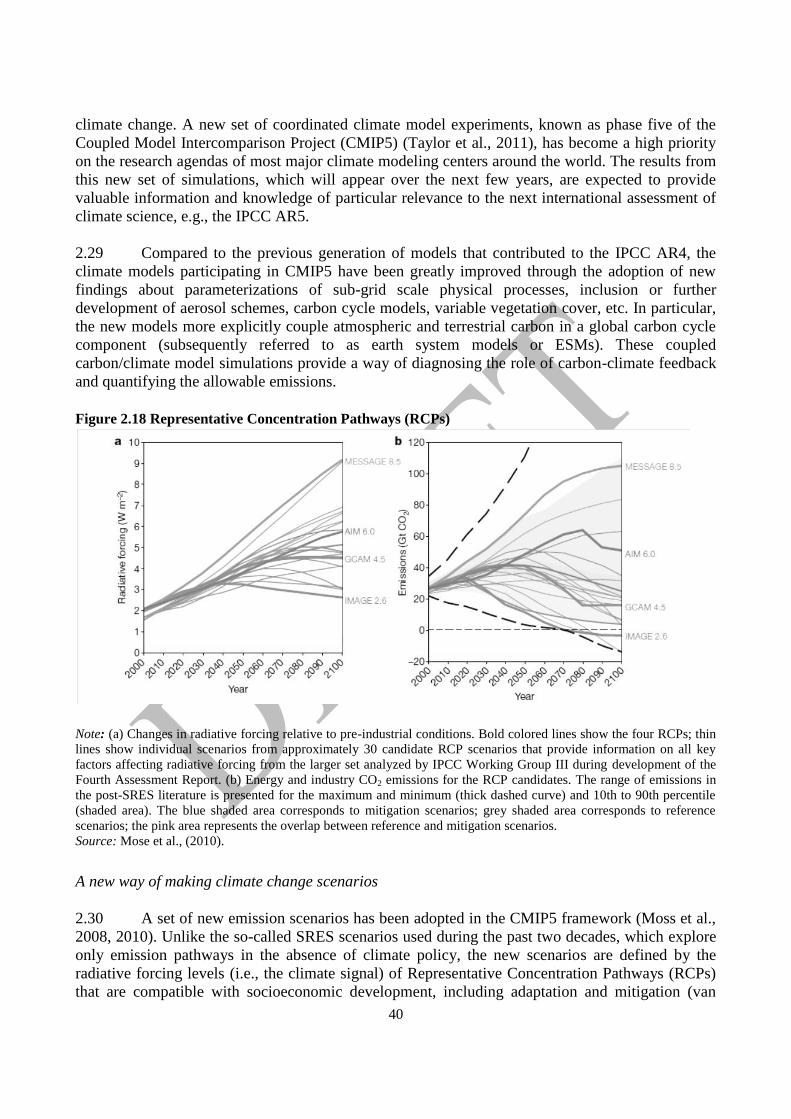
Figure 2.18 Representative Concentration Pathways (RCPs)
Note: (a) Changes in radiative forcing relative to pre-industrial conditions. Bold colored lines show the four RCPs; thin
lines show individual scenarios from approximately 30 candidate RCP scenarios that provide information on all key
factors affecting radiative forcing from the larger set analyzed by IPCC Working Group III during development of the
Fourth Assessment Report. (b) Energy and industry CO2 emissions for the RCP candidates. The range of emissions in
the post-SRES literature is presented for the maximum and minimum (thick dashed curve) and 10th to 90th percentile
(shaded area). The blue shaded area corresponds to mitigation scenarios; grey shaded area corresponds to reference
scenarios; the pink area represents the overlap between reference and mitigation scenarios.
Source: Mose et al., (2010).
A new way of making climate change scenarios
2.30 A set of new emission scenarios has been adopted in the CMIP5 framework (Moss et al.,
2008, 2010). Unlike the so-called SRES scenarios used during the past two decades, which explore
only emission pathways in the absence of climate policy, the new scenarios are defined by the
radiative forcing levels (i.e., the climate signal) of Representative Concentration Pathways (RCPs)
that are compatible with socioeconomic development, including adaptation and mitigation (van
41
Vuuren et al., 2010). Four RCPs are selected for CMIP5 experiments: one non-mitigated (RCP8.5),
and three taking into account various levels of mitigation (RCP6.0, RCP4.5 and RCP2.6), with
labels according to the approximate target radiative forcing at year~2100 (Figure 2.18). Each RCP
has been reviewed for internal consistency of the whole scenario, but only the information on
emissions, concentrations and land use are incorporated into the RCPs (Van Vuuren et al., 2010). In
comparison with the SRES, the RCPs provide more regionally detailed scenario information, such
as aerosol emissions, geographically explicit descriptions of land use and related emissions and
uptakes, and detailed specification of emissions by source type needed by new advances in climate
models. The RCPs establish a connecting and integrative thread that runs through the research
assessed by: the climate modeling community; the integrated assessment modeling community; and
the vulnerability, impacts and adaptation community.
A redefined focus on near-term changes
2.31 A new goal of the CMIP5 experiments aims specifically to provide decadal climate
predictions for the near term (out to about 2035). These experiments will be carried out with
atmosphere-ocean global climate models (AOGCMs) that are properly initialized for the ocean and
perhaps also sea ice and land surface, using either observations or initialization methods developed
recently. Some of the decadal simulations are expected to be performed using higher resolution in
order to better resolve regional climate and extremes. An enhanced resolution in such experiments
may enable a global horizontal grid scale as high as 50 km, which is equivalent to the scale of
regional climate models (RCMs), currently used in downscaling studies. These experiments will
also be able to better separate natural climate fluctuations from those that are anthropogenic in
origin.
The new scenarios to analyze mitigation outcomes
2.32 The CMIP5 experiments are intended to support the IPCC AR5, which is scheduled to be
published in 2013, although the work will continue beyond that date. Some early CMIP5 results
have already emerged. For example, in a recent study, Jones et al. (2011) reported results from
experiments employing ten AOGCMs and complex ESMs with an interactive carbon cycle from the
ENSEMBLES project (van der Linden and Mitchell, 2009) to simulate an ambitious mitigation
scenario of 21st century emissions, together with a contrasting medium-high emission scenario
from the SRES family (A1B). The study shows that the benefits of mitigation will not be realized in
temperature terms for several decades after emission reductions begin, and may vary considerably
between regions. The subset of the ESMs in the ensemble provides the allowable anthropogenic
carbon emissions under different scenarios as a direct model output.
Interpreting extreme events
2.33 A changing climate can lead to changes in the frequency, intensity or duration of an
extreme event, or, more generally to changes in the probability distribution function (PDF), and
eventually result in an unprecedented, previously unobserved extreme. From a meteorological point
of view, an extreme weather event is an event considered rare at a particular place and time of year.
An extreme event is commonly defined as one would normally be as rare or rarer than the 10th or
90th percentile of the observed probability density function for the meteorological phenomenon at
42
the location considered. When a pattern of extreme weather persists over time, such as during a
season, it may be classified as an extreme climate event, especially if it yields an average or total
that is in itself extreme (e.g., drought or heavy rainfall over a season). Extreme events usually
cannot be directly attributed to anthropogenic climate change, as there is always a finite chance the
event in question might have occurred naturally.
2.34 But extreme events are not interpreted purely from a meteorological point of view. A
weather or climate event, although not necessarily extreme in a statistical sense, may still have an
extreme impact, either by crossing a critical threshold in a social, ecological or physical system, or
because it occurs simultaneously with another event, which, in combination, leads to extreme
conditions or impacts. Conversely, not all extremes necessarily lead to serious impacts. The impact
of a tropical cyclone depends on where and when it makes landfall. Changes in phenomena, such as
monsoons, may affect the frequency and intensity of extremes in several regions simultaneously,
which indicates that the severity of an event may also depend on the overall geographical scale
being impacted. A critical or even intolerable threshold defined for a large region may be exceeded
before many, or any, of the smaller regions within it exceed local extreme definitions (e.g., local vs.
global drought).
Extremes occur even without climate change
2.35 Many weather and climate extremes are the result of natural climate variability (including
phenomena, such as El Niño), and natural decadal or multi-decadal variations in the climate provide
the backdrop for possible anthropogenic changes. Even if no anthropogenic changes in the climate
were to occur over the next century, a wide variety of natural weather and climate extremes would
still occur. Projections of changes in climate means are not always a good indicator of trends in
climate extremes. For example, observation and modeling show that precipitation intensity may
increase in some areas and seasons even as total precipitation decreases. Thus, an area might be
subject to both drier conditions and more flooding.
2.36 Tebaldi et al. (2006) illustrated this on a global scale (Figure 2.21). Based on a multi-
model analysis they found simulated increases in precipitation intensity for the end of the 21st
century (upper panel), along with a somewhat weaker and less clear trend of increasing dry periods
between rainfall events for the A1B scenario (lower panel). Precipitation intensity increases almost
everywhere, but particularly at middle and high latitudes where mean precipitation also increases
(Meehl et al., 2007). For the Arab region, the statistical signal is weak, but with an indication of
increasing risk of both increased precipitation intensity and increased length in dry day spells.

43
Figure 2.19 Changes in Extremes Based on Multi-Model Simulations from Nine Global Coupled
Climate Models
Note: Upper panel: Changes in spatial patterns of simulated precipitation intensity between two 20-year means (2080-
2099 minus 1980-1999) for the A1B scenario. Lower panel: Changes in spatial patterns of simulated dry days between
two 20-year means (2080-2099 minus 1980-1999) for the A1B scenario. Stippling denotes areas where at least five of
the nine models concur in determining that the change is statistically significant. Each model‘s time series was centered
on its 1980 to 1999 average and normalized (rescaled) by its standard deviation computed (after de-trending) over the
period 1960 to 2099. The models were then aggregated into an ensemble average at the grid-box level. Thus, changes
are given in units of standard deviations.
Source: Meehl et al. (2007).
Extreme impacts do not require extreme climate events
2.37 It is important to point out that events that may be perceived as extreme may actually be
due to the compound effect from: two or more extreme events; combinations of extreme events with
amplifying events or conditions; or combinations of events, which are not in themselves extreme,
Figure 10.18
44
but lead to an extreme event or impact when combined. The contributing events can be similar
(clustered multiple events) or very different. There are several varieties of clustered multiple events,
such as tropical cyclones generated a few days apart with the same path. Examples of compound
events resulting from events of different types are varied: for instance, high sea level coinciding
with tropical cyclone landfall, or a combined risk of flooding from sea level surges and
precipitation-induced high-river discharge (Van den Brink et al., 2005). Compound events can even
result from ―contrasting extremes,‖ for example, the projected near-simultaneous occurrence of
both droughts and heavy precipitation events mentioned above, or, more anecdotally, flash flooding
following bushfires due to fire-induced thunderstorms from pyrocumulus clouds (e.g., Tryhorn et al,
2008).
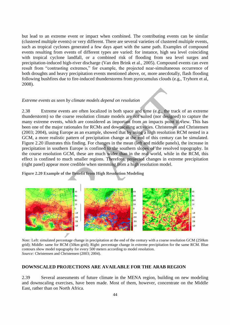
Extreme events as seen by climate models depend on resolution
2.38 Extreme events are often localized in both space and time (e.g., the track of an extreme
thunderstorm) so the coarse resolution climate models are not suited (nor designed) to capture the
many extreme events, which are considered as important from an impacts point if view. This has
been one of the major rationales for RCMs and downscaling activities. Christensen and Christensen
(2003; 2004), using Europe as an example, showed that by using a high resolution RCM nested in a
GCM, a more realistic pattern of precipitation change at the end of this century can be simulated.
Figure 2.20 illustrates this finding. For changes in the mean (left and middle panels), the increase in
precipitation in southern Europe is confined to the southern slopes of the resolved topography. In
the course resolution GCM, these are much wider than in the real world, while in the RCM, this
effect is confined to much smaller regions. Therefore, projected changes in extreme precipitation
(right panel) appear more credible when stemming from a high resolution model.
Figure 2.20 Example of the Benefit from High Resolution Modeling
Note: Left: simulated percentage change in precipitation at the end of the century with a coarse resolution GCM (250km
grid); Middle: same for RCM (50km grid); Right: percentage change in extreme precipitation for the same RCM. Blue
contours show model topography for every 500 meters according to model resolution.
Source: Christensen and Christensen (2003; 2004).
DOWNSCALED PROJECTIONS ARE AVAILABLE FOR THE ARAB REGION
2.39 Several assessments of future climate in the MENA region, building on new modeling
and downscaling exercises, have been made. Most of them, however, concentrate on the Middle
East, rather than on North Africa.

45
Box 2.3 Climate Models and Downscaling
The accuracy and representativeness of climate model data depends, among other factors, on the horizontal
resolution. It is therefore of importance to use a ―high enough‖ resolution to be able to represent features of
interest adequately, i.e. land/sea contrasts or fine scale topographical features
Figure 2.20 Index Map Color-Coding
Note: In this index map, color-coding is directly related to topographic height, with brown and yellow at the lower
elevations, rising through green, to white at the highest elevations. Blue areas on the map represent water. Image credit:
NASA/JPL-Caltech.
Source: http://photojournal.jpl.nasa.gov/catalog/PIA04965.
Figure 2.21 Model Topography at a Horizontal Resolution of 1° (about 100 km, top) and 0.2° (about 20
km., bottom)
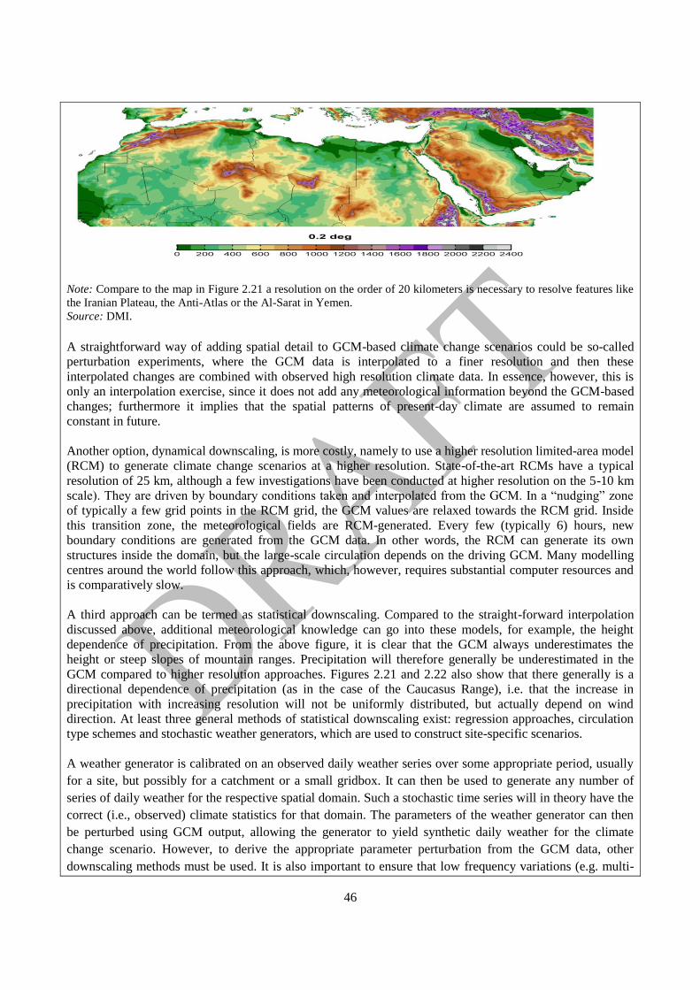
46
Note: Compare to the map in Figure 2.21 a resolution on the order of 20 kilometers is necessary to resolve features like
the Iranian Plateau, the Anti-Atlas or the Al-Sarat in Yemen.
Source: DMI.
A straightforward way of adding spatial detail to GCM-based climate change scenarios could be so-called
perturbation experiments, where the GCM data is interpolated to a finer resolution and then these
interpolated changes are combined with observed high resolution climate data. In essence, however, this is
only an interpolation exercise, since it does not add any meteorological information beyond the GCM-based
changes; furthermore it implies that the spatial patterns of present-day climate are assumed to remain
constant in future.
Another option, dynamical downscaling, is more costly, namely to use a higher resolution limited-area model
(RCM) to generate climate change scenarios at a higher resolution. State-of-the-art RCMs have a typical
resolution of 25 km, although a few investigations have been conducted at higher resolution on the 5-10 km
scale). They are driven by boundary conditions taken and interpolated from the GCM. In a ―nudging‖ zone
of typically a few grid points in the RCM grid, the GCM values are relaxed towards the RCM grid. Inside
this transition zone, the meteorological fields are RCM-generated. Every few (typically 6) hours, new
boundary conditions are generated from the GCM data. In other words, the RCM can generate its own
structures inside the domain, but the large-scale circulation depends on the driving GCM. Many modelling
centres around the world follow this approach, which, however, requires substantial computer resources and
is comparatively slow.
A third approach can be termed as statistical downscaling. Compared to the straight-forward interpolation
discussed above, additional meteorological knowledge can go into these models, for example, the height
dependence of precipitation. From the above figure, it is clear that the GCM always underestimates the
height or steep slopes of mountain ranges. Precipitation will therefore generally be underestimated in the
GCM compared to higher resolution approaches. Figures 2.21 and 2.22 also show that there generally is a
directional dependence of precipitation (as in the case of the Caucasus Range), i.e. that the increase in
precipitation with increasing resolution will not be uniformly distributed, but actually depend on wind
direction. At least three general methods of statistical downscaling exist: regression approaches, circulation
type schemes and stochastic weather generators, which are used to construct site-specific scenarios.
A weather generator is calibrated on an observed daily weather series over some appropriate period, usually
for a site, but possibly for a catchment or a small gridbox. It can then be used to generate any number of
series of daily weather for the respective spatial domain. Such a stochastic time series will in theory have the
correct (i.e., observed) climate statistics for that domain. The parameters of the weather generator can then
be perturbed using GCM output, allowing the generator to yield synthetic daily weather for the climate
change scenario. However, to derive the appropriate parameter perturbation from the GCM data, other
downscaling methods must be used. It is also important to ensure that low frequency variations (e.g. multi-
47
decadal variations) are adequately captured. Statistical downscaling approaches always require a very good
observational database to derive the statistical properties from. It is therefore not necessarily cheaper or
faster than running an RCM. It is also worth noting that downscaling methods generally cannot easily be
transported from one region to another. Just as with an RCM, the derived regional scenarios will depend on
the validity of the GCM data.
Eastern Mediterranean will become drier, especially in the rainy season
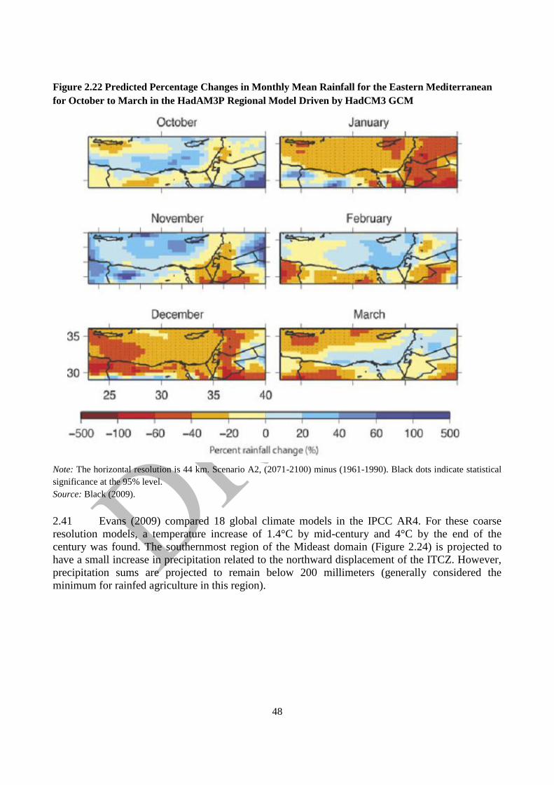
2.40 Figure 2.23 shows the change in the monthly mean rainfall over the eastern
Mediterranean. The most relevant finding is a significant decrease in precipitation (on the order of
40 percent) at the peak of the rainy season (December and January), not only for the West Bank and
Jordan, but also for the Eastern Mediterranean region as a whole (not shown). This is due to a
reduction in both the frequency and duration of rainy events. Before and after the rainy season, the
situation is less clear, with some areas projected to get wetter and others drier. These results are
broadly consistent with wider surveys of global models included in the IPCC AR4, which project a
decrease in annual total rainfall in the Middle East by the end of the 21st century (Lionello and
Giorgi, 2007; Kitoh et al., 2008; Evans 2009, Dai 2010) due to a reduction in the strength of the
Mediterranean storm track. The main mechanism is the northward displacement of this storm track
and, consequently, a reduction in the number of cyclones that cross the eastern Mediterranean basin
(Bengtsson et al., 2006).
48
Figure 2.22 Predicted Percentage Changes in Monthly Mean Rainfall for the Eastern Mediterranean
for October to March in the HadAM3P Regional Model Driven by HadCM3 GCM
Note: The horizontal resolution is 44 km. Scenario A2, (2071-2100) minus (1961-1990). Black dots indicate statistical
significance at the 95% level.
Source: Black (2009).
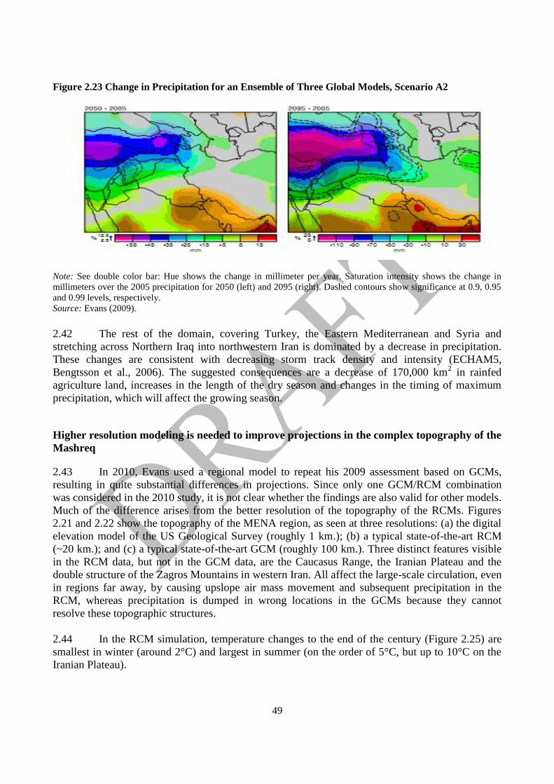
2.41 Evans (2009) compared 18 global climate models in the IPCC AR4. For these coarse
resolution models, a temperature increase of 1.4°C by mid-century and 4°C by the end of the
century was found. The southernmost region of the Mideast domain (Figure 2.24) is projected to
have a small increase in precipitation related to the northward displacement of the ITCZ. However,
precipitation sums are projected to remain below 200 millimeters (generally considered the
minimum for rainfed agriculture in this region).
49
Figure 2.23 Change in Precipitation for an Ensemble of Three Global Models, Scenario A2
Note: See double color bar: Hue shows the change in millimeter per year. Saturation intensity shows the change in
millimeters over the 2005 precipitation for 2050 (left) and 2095 (right). Dashed contours show significance at 0.9, 0.95
and 0.99 levels, respectively. Source: Evans (2009).
2.42 The rest of the domain, covering Turkey, the Eastern Mediterranean and Syria and
stretching across Northern Iraq into northwestern Iran is dominated by a decrease in precipitation.
These changes are consistent with decreasing storm track density and intensity (ECHAM5,
Bengtsson et al., 2006). The suggested consequences are a decrease of 170,000 km2 in rainfed
agriculture land, increases in the length of the dry season and changes in the timing of maximum
precipitation, which will affect the growing season.
Higher resolution modeling is needed to improve projections in the complex topography of the
Mashreq
2.43 In 2010, Evans used a regional model to repeat his 2009 assessment based on GCMs,
resulting in quite substantial differences in projections. Since only one GCM/RCM combination
was considered in the 2010 study, it is not clear whether the findings are also valid for other models.
Much of the difference arises from the better resolution of the topography of the RCMs. Figures
2.21 and 2.22 show the topography of the MENA region, as seen at three resolutions: (a) the digital
elevation model of the US Geological Survey (roughly 1 km.); (b) a typical state-of-the-art RCM
(~20 km.); and (c) a typical state-of-the-art GCM (roughly 100 km.). Three distinct features visible
in the RCM data, but not in the GCM data, are the Caucasus Range, the Iranian Plateau and the
double structure of the Zagros Mountains in western Iran. All affect the large-scale circulation, even
in regions far away, by causing upslope air mass movement and subsequent precipitation in the
RCM, whereas precipitation is dumped in wrong locations in the GCMs because they cannot
resolve these topographic structures.
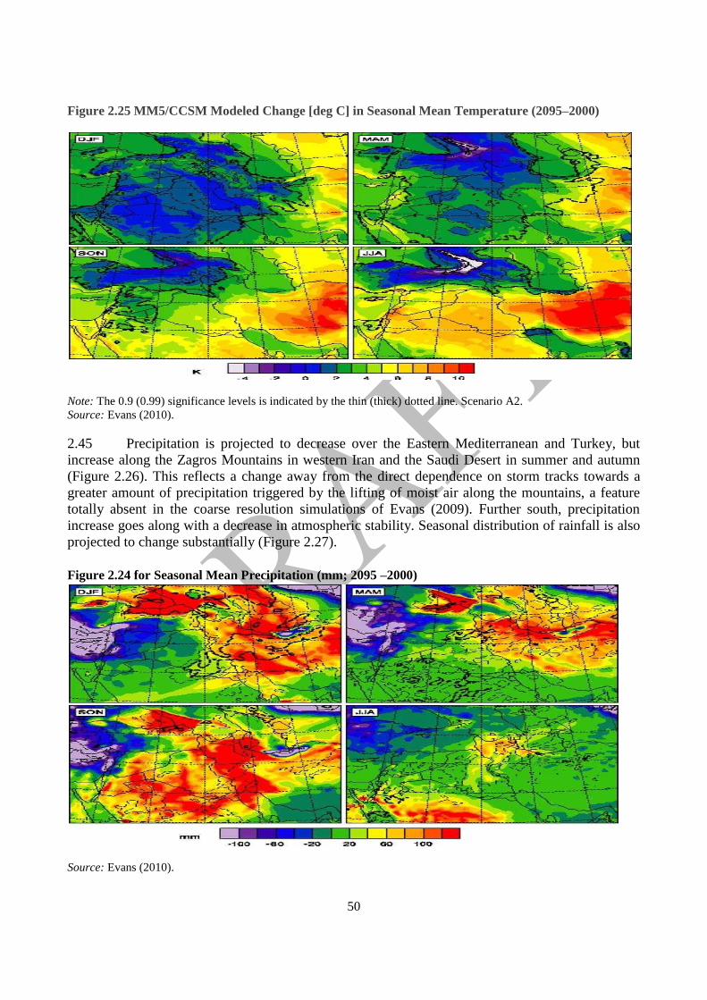
2.44 In the RCM simulation, temperature changes to the end of the century (Figure 2.25) are
smallest in winter (around 2°C) and largest in summer (on the order of 5°C, but up to 10°C on the
Iranian Plateau).
50
Figure 2.25 MM5/CCSM Modeled Change [deg C] in Seasonal Mean Temperature (2095–2000)
Note: The 0.9 (0.99) significance levels is indicated by the thin (thick) dotted line. Scenario A2.
Source: Evans (2010).
2.45 Precipitation is projected to decrease over the Eastern Mediterranean and Turkey, but
increase along the Zagros Mountains in western Iran and the Saudi Desert in summer and autumn
(Figure 2.26). This reflects a change away from the direct dependence on storm tracks towards a
greater amount of precipitation triggered by the lifting of moist air along the mountains, a feature
totally absent in the coarse resolution simulations of Evans (2009). Further south, precipitation
increase goes along with a decrease in atmospheric stability. Seasonal distribution of rainfall is also
projected to change substantially (Figure 2.27).
Figure 2.24 for Seasonal Mean Precipitation (mm; 2095 –2000)
Source: Evans (2010).
51
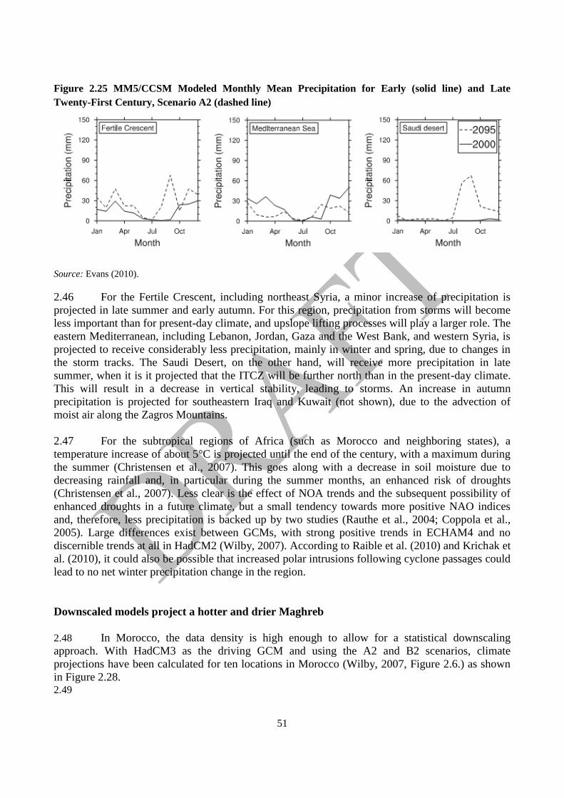
Figure 2.25 MM5/CCSM Modeled Monthly Mean Precipitation for Early (solid line) and Late
Twenty-First Century, Scenario A2 (dashed line)
Source: Evans (2010).
2.46 For the Fertile Crescent, including northeast Syria, a minor increase of precipitation is
projected in late summer and early autumn. For this region, precipitation from storms will become
less important than for present-day climate, and upslope lifting processes will play a larger role. The
eastern Mediterranean, including Lebanon, Jordan, Gaza and the West Bank, and western Syria, is
projected to receive considerably less precipitation, mainly in winter and spring, due to changes in
the storm tracks. The Saudi Desert, on the other hand, will receive more precipitation in late
summer, when it is it projected that the ITCZ will be further north than in the present-day climate.
This will result in a decrease in vertical stability, leading to storms. An increase in autumn
precipitation is projected for southeastern Iraq and Kuwait (not shown), due to the advection of
moist air along the Zagros Mountains.
2.47 For the subtropical regions of Africa (such as Morocco and neighboring states), a
temperature increase of about 5°C is projected until the end of the century, with a maximum during
the summer (Christensen et al., 2007). This goes along with a decrease in soil moisture due to
decreasing rainfall and, in particular during the summer months, an enhanced risk of droughts
(Christensen et al., 2007). Less clear is the effect of NOA trends and the subsequent possibility of
enhanced droughts in a future climate, but a small tendency towards more positive NAO indices
and, therefore, less precipitation is backed up by two studies (Rauthe et al., 2004; Coppola et al.,
2005). Large differences exist between GCMs, with strong positive trends in ECHAM4 and no
discernible trends at all in HadCM2 (Wilby, 2007). According to Raible et al. (2010) and Krichak et
al. (2010), it could also be possible that increased polar intrusions following cyclone passages could
lead to no net winter precipitation change in the region.
Downscaled models project a hotter and drier Maghreb
2.48 In Morocco, the data density is high enough to allow for a statistical downscaling
approach. With HadCM3 as the driving GCM and using the A2 and B2 scenarios, climate
projections have been calculated for ten locations in Morocco (Wilby, 2007, Figure 2.6.) as shown
in Figure 2.28. 2.49
52
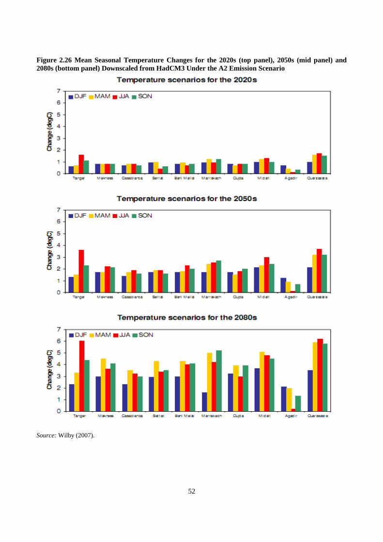
Figure 2.26 Mean Seasonal Temperature Changes for the 2020s (top panel), 2050s (mid panel) and
2080s (bottom panel) Downscaled from HadCM3 Under the A2 Emission Scenario
Source: Wilby (2007).
53
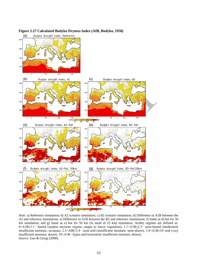
Figure 2.27 Calculated Budyko Dryness Index (AIB, Budyko, 1958)
Note: a) Reference simulation; b) A2 scenario simulation; c) B2 scenario simulation; d) Difference in A1B between the
A2 and reference simulations; e) Difference in A1B between the B2 and reference simulations; f) Same as d) but for 50
km simulation; and g) Same as e) but for 50 km (in stead of 25 km) simulation. Aridity regimes are defined as:
0<A1B≤1.1− humid (surplus moisture regime; steppe to forest vegetation), 1.1<A1B≤2.3− semi-humid (moderately
insufficient moisture; savanna), 2.3<AIB≤3.4− semi-arid (insufficient moisture; semi-desert), 3.4<A1B≤10−arid (very
insufficient moisture; desert), 10<A1B− hyper-arid (extremely insufficient moisture; desert).
Source: Gao & Giorgi (2008).
54
2.50 Projected temperature increases are smallest in Agadir (coastal station) and largest in
Ouarzazate in the Atlas Mountains, where summer temperatures are projected to increase by more
than 6°C by the 2080s. Along with this, the frequency and severity of heat waves will increase.
According to Wilby (2007), almost 50 days per year with a maximum above 35°C in Settat (near
the coast) and Beni Mellal (in the Atlas foothills) are projected by the end of the century. Except in
Agadir and Marrakech, less rainfall is projected, ranging from about a 25 percent decrease in the
south to approximately a 40 percent decrease in the agro-economic zone in the north.
2.51 Figure 2.29 shows an assessment of drought in the Mediterranean region (including
substantial parts of the Maghreb) for present-day climate and two scenarios, each at two different
horizontal resolutions (Gao and Giorgi, 2008). Both scenarios show the drought risk around the
Mediterranean Sea increasing from west to east, which is worst in the Levante, but notable also in
other regions, including southern Europe.
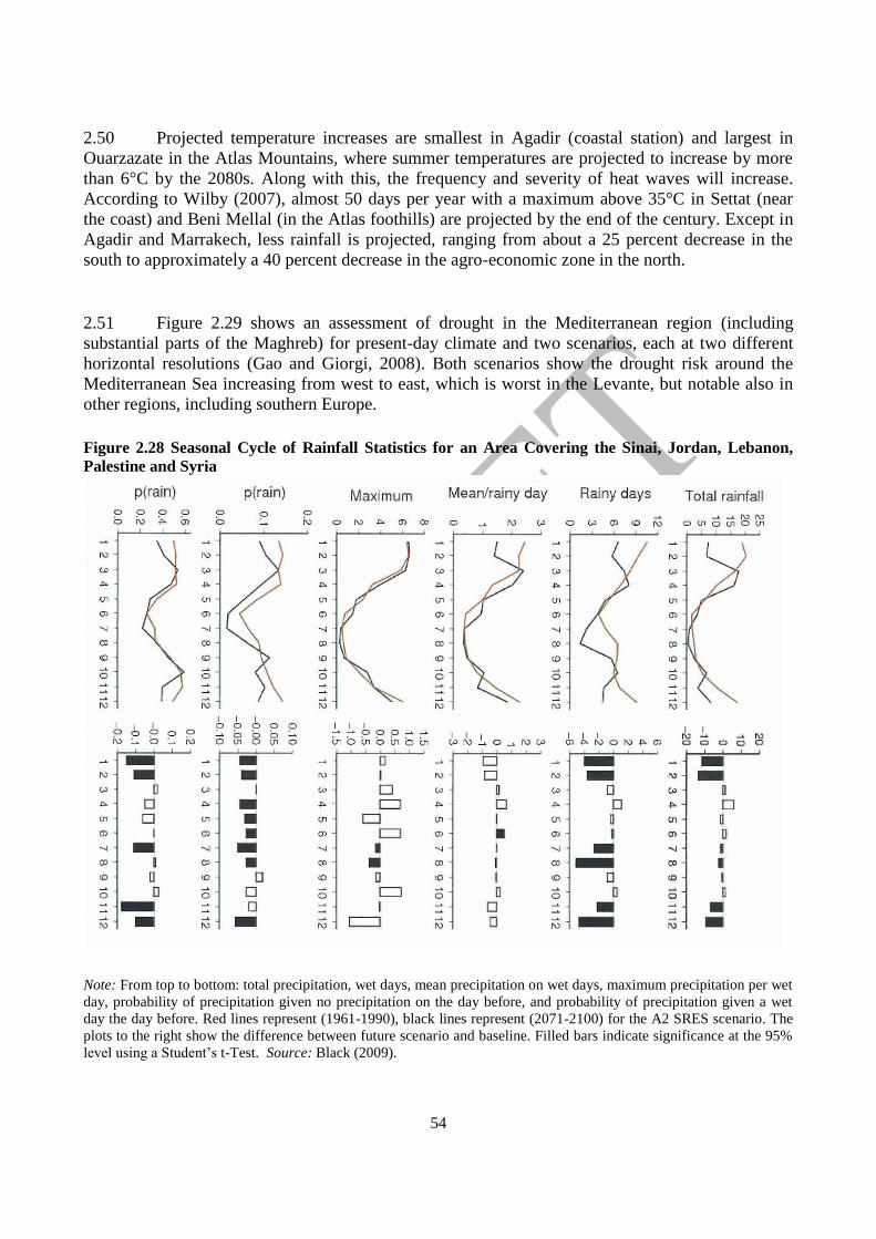
Figure 2.28 Seasonal Cycle of Rainfall Statistics for an Area Covering the Sinai, Jordan, Lebanon,
Palestine and Syria
Note: From top to bottom: total precipitation, wet days, mean precipitation on wet days, maximum precipitation per wet
day, probability of precipitation given no precipitation on the day before, and probability of precipitation given a wet
day the day before. Red lines represent (1961-1990), black lines represent (2071-2100) for the A2 SRES scenario. The
plots to the right show the difference between future scenario and baseline. Filled bars indicate significance at the 95%
level using a Student‘s t-Test. Source: Black (2009).
55
Agricultural lands are threatened by increasing aridity in the Mashreq
2.52 Figure 2.30 shows precipitation statistics for an area consisting of the Sinai, Jordan,
Lebanon, Palestine and Syria. Most prominent are a (statistically significant) decrease in the
number of rainy days, both following a dry or a wet day, and a general decrease in winter rainfall.
According to the GCMs in Christensen et al. (2007) and RCM experiments by Önol and Semazzi
(2009), temperatures in the region will increase on the order of 2°C in winter and up to 6°C in the
inland regions in summer. A reduction in winter precipitation on the order of 25 percent and an
increase of drought duration by up to 60 percent are expected based on the A1B scenario (Kim and
Byun, 2009). The authors also predict a northward expansion of the Arabian Desert and an increase
of autumn precipitation over the Fertile Crescent by up to 50 percent.
2.53 Although less favorable than for Morocco, the data density is sufficient to allow for
statistical downscaling by stations in Amman (Jordan), Kamishli (Syria) and Kfardane (Lebanon).
While for Kamishli, the present-day climate can be reconstructed quite well, results are less
convincing for Amman. This may be due to missing data and problems due to station relocation and
urban growth (Smadi and Zghoul, 2006). Depending on scenario and location, temperature
increases by 3-4°C (A2) and 2-3°C (B2), respectively, are obtained (Wilby, 2010), while rather
large decreases in precipitation are projected — up to 50 percent near the coast (Lattakia, Syria) and
around 15-20 percent inland (for example, in Palmyra, Syria). Note that this reduction in
precipitation takes place almost entirely during the winter, as generally no precipitation exists at all
during summer under present-day conditions.
2.54 As mentioned above, it has been suggested (Evans and Geerken, 2004) that the limit for
rainfed agriculture lies close to average annual precipitation of 200 millimeters per year. Taking
Amman as an example (average precipitation 1961-1990 was 260 millimeters), this suggests that
agriculture would no longer be possible in 2080. However, due to the large interannual variability
(coefficient of variation in Amman is 38 percent, which implies that there is a 1/3 chance for an
annual sum under 200 millimeters even in present-day conditions), agriculture could cease to be
economically viable considerably earlier. Based on HadCM3 data and the A2 scenario, the chance
of a dry year (<200 millimeters) would be 50 percent around 2020 rising to 80 percent around 2060.
This finding is consistent with previous studies that suggest that the 200 millimeters isohyet could
move on the order of 75 km northward by the end of the century (Evans, 2009). If precipitation is
too low, agriculture is traditionally replaced by grazing. The same scenario projects an increase in
the dry season length from 6 to 8 months by 2080 for Amman, which potentially poses a problem to
the herders.
2.55 Based on Christensen et al. (2007), GCMs suggest a temperature increase of 4°C in
winter and 6-7°C in summer. But unlike in the Maghreb and Levante regions, there is little
agreement between the models. No clear climate change sign is found for precipitation, with
indications for slightly wetter conditions in the south and drier conditions in the north, related to the
northward shift of the ITCZ.
2.56 Figure 2.31 shows results from another RCM simulation covering the Arabian Peninsula
and neighboring regions. Apart from the coastal plains in Yemen, Oman and Somalia, where the
salt marshes remain comparatively humid and therefore experience less warming, relatively uniform
warming is projected. For precipitation, changes are small in areas that are already arid under
56
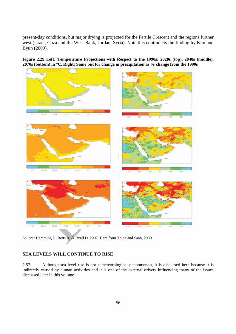
present-day conditions, but major drying is projected for the Fertile Crescent and the regions further
west (Israel, Gaza and the West Bank, Jordan, Syria). Note this contradicts the finding by Kim and
Byun (2009).
Figure 2.29 Left: Temperature Projections with Respect to the 1990s: 2020s (top), 2040s (middle),
2070s (bottom) in °C. Right: Same but for change in precipitation as % change from the 1990s
Source: Hemming D, Betts R, & Ryall D. 2007. Here from Tolba and Saab, 2009.
SEA LEVELS WILL CONTINUE TO RISE
2.57 Although sea level rise is not a meteorological phenomenon, it is discussed here because it is
indirectly caused by human activities and it is one of the external drivers influencing many of the issues
discussed later in this volume.
57
Global mean sea level has been observed to have steadily increased since 1870
2.58 The sea level of the sea at the shoreline is determined by many factors that operate over a
great range of temporal scales: hours to days (tides and weather), years to millennia (climate) and
longer. The land itself can rise and fall and such regional land movements must be accounted for
when using tide gauge measurements for evaluating the effect of oceanic climate change on coastal
sea levels. Coastal tide gauges indicate that the global average sea level rose during the 20th
century. Since the early 1990s, sea level has also been continuously observed by satellites, with
near-global coverage. Satellite and tide gauge data agree at a wide range of spatial scales and show
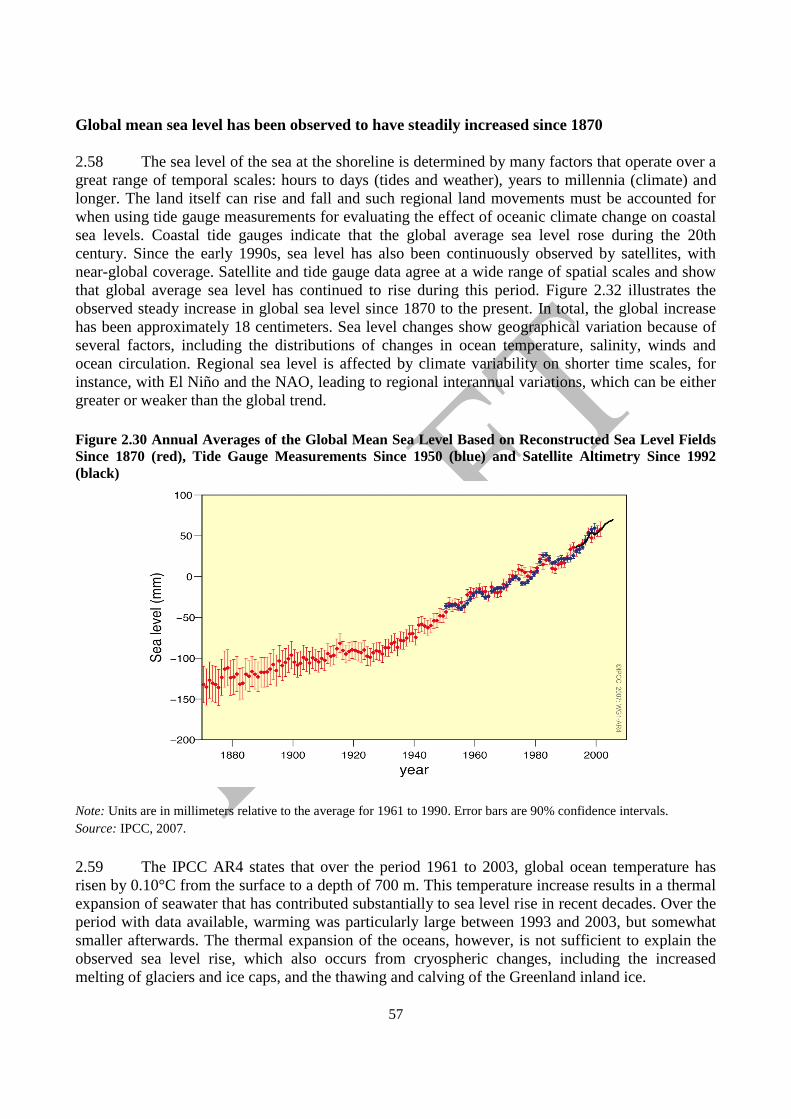
that global average sea level has continued to rise during this period. Figure 2.32 illustrates the
observed steady increase in global sea level since 1870 to the present. In total, the global increase
has been approximately 18 centimeters. Sea level changes show geographical variation because of
several factors, including the distributions of changes in ocean temperature, salinity, winds and
ocean circulation. Regional sea level is affected by climate variability on shorter time scales, for
instance, with El Niño and the NAO, leading to regional interannual variations, which can be either
greater or weaker than the global trend.
Figure 2.30 Annual Averages of the Global Mean Sea Level Based on Reconstructed Sea Level Fields
Since 1870 (red), Tide Gauge Measurements Since 1950 (blue) and Satellite Altimetry Since 1992
(black)
Note: Units are in millimeters relative to the average for 1961 to 1990. Error bars are 90% confidence intervals.
Source: IPCC, 2007.
2.59 The IPCC AR4 states that over the period 1961 to 2003, global ocean temperature has
risen by 0.10°C from the surface to a depth of 700 m. This temperature increase results in a thermal
expansion of seawater that has contributed substantially to sea level rise in recent decades. Over the
period with data available, warming was particularly large between 1993 and 2003, but somewhat
smaller afterwards. The thermal expansion of the oceans, however, is not sufficient to explain the
observed sea level rise, which also occurs from cryospheric changes, including the increased
melting of glaciers and ice caps, and the thawing and calving of the Greenland inland ice.
Figure TS.18
58
2.60 Large-scale, coherent trends of salinity have also been observed over the last few
decades. All available data point toward a freshening in subpolar latitudes and a salinification in
parts of the subtropical and tropical oceans. These trends are consistent with changes in
precipitation and evaporation and probably an increased freshwater flow into the Arctic from river
runoff and thawing land ice. Furthermore, oceans have become more acidic and, as a consequence,
the amount of emitted carbon dioxide taken up by the oceans has decreased.
2.61 Recent expert meetings (e.g., from the climate conference held in Copenhagen in
December 2009) discussed whether the IPCC AR4 had underestimated the amount of sea level rise
and that ocean warming is about 50 percent greater than the IPCC had previously reported. Material
presented at the above conference suggested that the rate of sea level rise increased during the
period from 1993 to the present, mainly due to the growing contribution of ice loss from Greenland
and Antarctica. Observations show that the area of the Greenland ice sheet at freezing point or
above for at least one day during the summer period increased by 50 percent during the period 1979
to 2008, particularly during the extremely warm summer of 2007 (Steffen and Huff, 2009; Mote,
2007).
2.62 Ice sheets may also lose mass through ice discharge, which is also sensitive to regional
temperature. The best estimate is that the Greenland ice sheet has been losing mass at a rate of 179
Gt/year since 2003, corresponding to a contribution to global mean sea level rise of 0.5
millimeters/year (AMAP, 2009). This is approximately twice the amount estimated by the IPCC in
2007.
Climate models project sea level will continue to rise in the 21st century
2.63 Climate models are consistent with the ocean observations and indicate that thermal
expansion is expected to continue to contribute significantly to sea level rise over the next 100
years. New estimates suggest a sea level rise of around one meter or more by 2100 (IOP, 2009).
Since deep ocean temperatures change slowly, thermal expansion would continue for many
centuries even if atmospheric greenhouse gas concentrations were stabilized today.
2.64 In a warmer climate, models suggest that the ice sheets could accumulate more snowfall,
which would lower the sea level. However, in recent years, any such tendency has probably been
outweighed by accelerated ice flow and greater discharge. The processes of accelerated ice flow are
not yet completely understood, but are likely to continue to result in overall net sea level rise from
the two large ice sheets of Greenland and Antarctica.
2.65 The greatest climate- and weather-related impacts of sea level are due to extremes
associated with tropical cyclones and mid-latitude storms, on time scales of days and hours. Low
atmospheric pressure and high winds produce large local sea level excursions called ―storm surges,‖
which are especially serious when they coincide with high tide. Changes in the frequency of the
occurrence of these extreme sea levels are affected both by changes in mean sea level and in the
meteorological phenomena causing the extremes.
59
FROM CLIMATE MODELS TO IMPACT ANALYSES
More effort is needed to develop good impact models to translate climate to potential impacts
2.66 The previous sections of this chapter have attempted to explain what is understood about
observed and projected climate change, and have emphasized the strengths and limitations of both
observational data and the climate models used to make projections. We know that the Earth is
warming and that the atmosphere is becoming more unstable as a result. Great uncertainty remains
about the precise magnitude of changes in climate and weather patterns at any given location and
time. Some of this uncertainty derives from the inherently chaotic nature of the weather and climate
and from limitations in the models, but much is derived from uncertainty about future human
actions that release greenhouse gases and change land cover. Despite these uncertainties, decisions
still have to be made about water management, agricultural practices, land use and infrastructure,
where the consequences of the decisions extend well into what we know will be significantly
changed climates. These decisions are often guided by ―impact models‖ that, among many other
factors, take into account climate and climate variability. These were typically guided by climate
observations from the recent past (e.g., 1961 to 1990 weather data), but the past is no longer a good
prophesy of the future. The challenge is to find ways of representing both the understanding of
future climate and the uncertainties in models of water use, decisions about land use and
infrastructure design.
2.67 A number of steps must be taken when deciding how to incorporate future climate change
and variability into impact models. The first is to assess how the impact model considers current
climate variability. Many models, e.g., many economic models, treat climate as a constant and
factor climate variability into a general error term or safety factor, as in bridge and building design.
In some cases, the design of these decision processes will have to be reassessed. Can the safety
margins simply be extended? Will these still lead to effective and efficient decisions? In some
cases, new approaches to modeling impacts will be needed. Other decisions are based on detailed
models of stream flow or agricultural productivity, which are driven by detailed inputs of
meteorological data. In these cases, the challenge is to replace inputs from the recent past with
inputs from well selected models of the future. But many of these models require data at a much
finer resolution than can be produced by GCMs and even RCMs and at time scales (e.g., hourly or
daily data) that are often not available from modeling runs.
The challenge of output resolution –in both space and time scales
2.68 The horizontal resolution of GCMs is typically 100-200 km, which is usually too coarse
for direct use by impact models. Climate projections with higher spatial resolution can be obtained
by dynamical downscaling, using high-resolution RCMs driven by initial and boundary conditions
provided by GCMs (e.g., Rummukainen, 2010). This improved resolution makes it possible to
include subgrid variability, like small-scale topography, and to resolve sub-grid processes to
improve the modeling of regional precipitation, for example. Indeed, a number of studies show that
the results from impact models using downscaled climate information can be quite different from
results directly based on GCM output (e.g., Mearns et al., 2001; Olesen et al., 2007).
2.69 Different GCMs and RCMs use different physical formulations to describe atmospheric
processes, interactions between the atmosphere and the land and oceans, etc., and, thus, provide
60
different projections of future climate. The spread of results from these different models represents
an uncertainty regarding future climates that must be accounted for by impact modelers. Too often
impact models have been driven by the results of a single GCM or RCM. However, the
uncertainties are now being explored by ensemble simulations applying different combinations of
GCMs and RCMs (e.g., Christensen et al., 2007b; Kjellström et al., 2010). One way of directly
including this uncertainty is to calculate the probability distribution of important outputs (e.g., daily
maximum temperatures) based on the information from the full set of model simulations (Déqué
and Somot, 2010). In recent studies, the contribution of individual models to the probability
distribution has been weighted according to their performance with respect to a given set of metrics
(Christensen et al., 2010). The weighting procedure itself adds an extra source of uncertainty and
the method is still being explored. For example, the ability of a model to predict present-day climate
could be seen as an indication that it will also be able to predict future climate. However, feedback
mechanisms that were important in the past could be less important in a future climate with a
different forcing, so the weightings themselves may not be appropriate (Christensen et al., 2008;
Reifen and Toumi, 2009). In addition, models may perform differently for different regions. The
Coordinated Regional climate Downscaling Experiment (CORDEX) initiative will study this and
offer new regional projections for a number of regions across the world, including the Arab region,
although not as a single entity, but rather distributed across several proposed regional domains
(Giorgi and Asrar, 2009).
2.70 The probability distributions discussed in the previous paragraph usually apply to a point
in time. However, for impact studies, time series are generally needed, making the probabilistic
approach more difficult. Large-scale community efforts have addressed how to pick the most
relevant climate information from an ensemble of model simulations (Christensen et al., 2007b;
Christensen et al., 2009). As for the weighting procedure, the selection of individual models is in
itself a source of uncertainty and should be done carefully to avoid biasing the resulting analyses.
2.71 Most downscaling methods combine climate model output with observed data. In this
way, local features not captured by the climate model can be incorporated in the scenario data,
allowing the impact model to be used with data in the form that it was developed and tailored to.
The most appropriate method of preparing climate scenario data depends on the local region and on
the specific needs of the impact models.
2.72 Any requirement to use time series in order to calibrate and validate an impact model
prevents the direct use of GCM or RCM data, as the climate models do not reproduce sequences of
real weather events. The models are not designed nor meant to be able to do this. Instead, a climate
model is constructed with the aim of being able to reproduce climate, which, in a narrow sense, is
usually defined as the average weather or, more rigorously, as the statistical description in terms of
the mean and variability of relevant quantities over a period of time, ranging from months to
thousands or millions of years. The classical period for averaging these variables is 30 years, as
defined by the WMO. The relevant quantities are most often surface variables, such as temperature,
precipitation and wind. Climate in a wider sense is the state of the climate system, including a
statistical description. Even downscaled climate change information is still not akin to a weather
prediction. Many climate variables in the model output are systematically offset and need to be bias
corrected, which requires observational data.
2.73 Methods to transform climate model output into the impact application are therefore
called for. The climate change scenarios can be further downscaled to a regional or local level by
61
applying a weather generator (WG) approach. For example, a stochastic WG based on the series
approach (Racsko et al., 1991) has been proven to give a realistic representation of the duration of
wet and dry days and, thus, the duration of droughts, while the frequently applied Markov chain
models (Semenov et al., 1998) is less successful in achieving this. Such an approach has the benefit
of allowing for a good representation of current climatic conditions by calibrating the WG to
observed data, and allowing not only the inclusion of changes in mean climate from the RCMs (or
GCMs), but also changes in climatic variability. This approach also has the flexibility to generate
longer and multiple time series of synthetic weather data for use in impact models, thus allowing for
better quantifying the variability in response to climate change.
2.74 Even if suitable time series of weather data are generated to drive an impact model, the
question remains as to what extent is the impact model itself calibrated and tested for weather
conditions beyond those experienced in observed conditions. This should be clarified when the
model is used under climate change conditions, in particular when addressing values well outside
past experiences or when extreme events are being assessed.
From weather forecasting to seasonal-to-decadal prediction
2.75 A climate model is designed to be able to capture the statistical properties of the
geographically and temporarily varying weather that characterizes climate; it is not designed to
predict the actual weather. A weather prediction or forecast, on the other hand, is typically
formulated as a categorical statement about the state of the weather within a certain time frame,
typically up to 10 or 15 days (medium-range forecasts). More recently, monthly and seasonal time
scale forecasts are also provided by many centers. These forecasts typically provide qualitative
assessments of the most likely weather development, primarily based on long-term variations, e.g.,
expectation of droughts or moist conditions. A commonality between all forecasts is the
dependency on a well-defined initial state that must have its origin in an observed state of the
atmospheric (or more broadly the climate) system. This typically involves some kind of data
assimilation system by which the forecast model is constrained towards the observed evolution of
the weather and/or oceanic state, moist or dry land surfaces, etc. The techniques to adequately
combine modeled information, typically represented on a grid, with point measurements at which
most observations are made, comprise a large research field of their own.
2.76 In climate modeling, the model typically begins from an idealized initial state, which
aims to represent conditions ―typical‖ for the period it is intended to represent, often pre-industrial
conditions where the levels of greenhouse gases and anthropogenic aerosol loads in the atmosphere
were low. Then known or estimated external forcings from the emission of greenhouse gases and
aerosols, varying solar insolation, volcanism and other drivers (e.g., land use) are introduced into
the freely running model. In this way, a modeled representation of the evolution of the climate since
the industrial revolution is made. But the state of the climate in such a model for a particular
decade, say 2001-2010, is not meant to be compared with the real world for that decade. The model
is designed to capture the changing characteristics of major phenomena such El Niños decadal
fluctuations in monsoons, the NAO, etc. but not forecast particular events.
2.77 This is a problem when the challenge is to address the near future climate development
because natural fluctuations on the decadal time scale are major determinants. In essence, the
probable evolution of climate over the next three to four decades is more difficult to depict than the
62
climate at the end of the century under a prescribed emission scenario. This is very often forgotten
when impact assessments are called for.
2.78 Some predictability in the atmosphere on seasonal, interannual and decadal time scales
can arise from internally generated natural climate variability—often connected to oceanic
variability—and certain types of external forcing (solar and volcanic eruptions). Internal variability
that results in, e.g., extensive, long-lasting, upper ocean temperature anomalies, has the potential to
provide seasonal, interannual and even decadal predictability in the overlying atmosphere, both
locally and remotely through atmospheric ―teleconnections.‖ These teleconnections can guide
predictions for the next few seasons. The question of whether or not skill extends to forecasts for
the following decade and beyond is a scientific ―hot topic‖ and currently a central issue in the
upcoming AR5.
2.79 The magnitude of the changes in the atmosphere associated with any decadal
predictability at a specific location is extremely small compared with the size of the day-to-day
variability linked to changes in weather at that same location. Thus, the decadal signal is difficult to
recognize amongst the much larger variability arising from unrelated changes in weather. So while
the decadal signal can underpin predictability in changes to decadal averages in climate variables,
the same signal provides little if any enhancement to our ability to forecast weather.
2.80 The level of predictability and apparent predictive skill arising from both internal and
external forcing can vary markedly from place-to-place and from variable-to-variable. Recent
research (see e.g., Meehl et al. (2009), Murphy et al. (2010), Latif et al. (2010) and Hurrell et al.
(2010)) indicates that predictability is absent or very limited in some variables in most locations
over the surface of the earth. So we cannot accurately predict all aspects of the climate over the
coming decades even if we could perfectly resolve all the technical issues confronted when
developing and conducting predictions. The nature of the climate system precludes the possibility of
reliable decadal predictions of some climate variables in some locations. In such cases, the best
estimate that can be provided for the quantities and regions in question for future decades is the
information contained in historical climate records.
The practice of impact modeling
2.81 The best choices for integrating climate modeling projections with impact modeling
depends on location, time period and application, and is best made through the cooperation of
climate modeling and impact specialists. It is not possible to discuss the myriad of options in this
chapter, but in Annex 1, we provide some guidelines as to how a team responsible for developing
impact models to guide decisions that are likely to be affected by climate change might step through
the process of developing advice guided by the best available understanding of future climates.
63
APPENDIX B.1 DEALING WITH CLIMATE RISKS – A CHECKLIST
This checklist is designed to guide the leadership of a program or large sectoral or cross-sectoral project that is assessed as being subject to climate
risks. Examples include the construction of a new dam, a major rural road upgrade, the design of an agricultural irrigation program, or a major
coastal tourism development. The checklist is designed to assist in incorporating climate risk, including climate change, in the program design. It
is essentially a top-down approach to adaptation that unfortunately so often brings adaptation considerations rather late to the decision process
(Wilby & Dessai, 2010). This is not the only, nor necessarily, the most effective, approach to adaptation planning (see World Bank World
Development Report 2010; Lempert et al., 2004; Wilby & Dessai, 2010; Hallegate et al., 2011 for a wider discussion of adaptation in the context
of wider development goals). However, the circumstances described above are common in development planning and especially that which
focuses on infrastructure.
Note: The order of the checklist is such that items nearer the top are most likely to precede those below, but this is NOT a purely sequential
process.
1. Assess where you stand in the decision process
a. If the decision process is in its early stages, then
follow a process to identify goals and needs of
stakeholders, and the range of adaptation options
and criteria by which they may be evaluated. This
is the most desirable situation, but this checklist
cannot elaborate this open-ended and case-
specific process any further.
Clearly, this is the best stage to begin considering adaptation actions. It allows the
full range of climate-resilient options to be considered. See the references in the
introductory paragraph for guidance.
b. Are the core features of the design in place? If so,
what information relating to future climate might
challenge these decisions?
Here, the assumption is that adaptation to climate risk and climate change is a
component of a wider development objective, i.e., this is not a ―stand-alone‖
adaptation project.
c. What are the feasible options for the modification
or fine-tuning of the existing design?
These options need to be identified so that appropriate decisions can be made
about how much assessment of the climate risks is needed. At this point, simple
64
―rules-of-thumb‖ about climate change may need to be applied. For example,
using expert judgment to assess the effect of a warmer climate with more variable
precipitation on the proposed project.
d. What is the time horizon relevant to the decision
process?
The time horizon is not necessarily limited to the longevity of a piece of
infrastructure. For example, implementing improved flood resistance of a planned
road system may be sufficient for the normal design horizon for roads, but it could
also lead to denser settlement in inherently flood-prone areas, leading to
unacceptable outcomes in the climates of the more distant future.
2. What does the latest IPCC Report and
subsequent commentaries and updates say about
your project location and sector(s)?
The IPCC Reports will contain a summary of the current climate, observed
changes, climate change projections and the possible impacts affecting your
region.
www.ipcc.ch
3. Are more recent (since the most recent IPCC
Report) or more nationally or regionally explicit
assessments available?
a. Many countries have their own national
assessments of climate change and its impacts
Check National Communications to the UNFCCC at
http://unfccc.int and search for National Reports
b. Assess the knowledge base and validity of all
assessments
Many national and sub-national reports are summaries from the IPCC with little
additional information
c. Identify major discrepancies (if any) between the
regional/explicit assessments of the IPCC and
seek to establish an explanation
Discrepancies may arise because of newer information, more regionally specific
information, different sources of information, or errors and misinterpretations.
4. Establish a climate base line The climate baseline is a description of the current climate (often a 30 year period,
such as 1961-1990), including averages, variability and trends. It is used to both
establish the current conditions and most modeled projections (next section) are
interpreted as changes to this baseline.
a. Seek cooperation and input from the national
meteorological office and similar authorities, e.g.,
Baseline climate information may exist in a form that is not publically available.
E.g. data may not exist in digitized form or if digitized, basic quality control may

65
for sea level monitoring still be lacking.
b. Decide upon the variables that may affect the
outcome and design of the project
They are not only temperature and precipitation. They are more likely to be
complex variables, such as run-off, dry spells, rainfall intensity, wind storms and
dust storms. Some of these variables are available from GCM modeling, while
others will have to be derived through secondary modeling.
c. Explore the existing public data bases for both
station and gridded data
See references in this chapter for coverage of the Arab region.
d. Calculate averages, trends and measures of
variability for the variables of interest
See the World Bank Climate Portal where much of this information is available
(http://sdwebx.worldbank.org/climateportal/)
e. Share the base line data with appropriate experts
(sectoral and climate) and review – revisit
Section 1 above if necessary
These analyses may give insights to additional options in the project design
5. Establish the relevant range of climate
projections
a. Currently, 22 IPCC AR4 models form a core set
and are available from the sources listed opposite.
List of sources for 22 GCMs
b. Assess whether particular scenarios should be
chosen (i.e., A1B, A2, B1, B2). Note that for
projections in the near term (next few decades),
the choice scenario makes little difference.
The A1B is closest to our current trajectory. A common pairing is B1 (most
effective mitigation) with A1B (in-effective mitigation).
c. Do not reject any GCM unless data is missing, or
an authoritative climatological reason indicates it
is inappropriate.
Some users seek a single ―best‖ GCM for their region. This is unwise as the
criteria for choosing the best are unclear; one GCM might project current
precipitation better in your region, while another matches temperatures better.
Also, the ability to project current climate does not necessarily indicate the ability
to project future scenarios.
d. Check the performance of each GCM selected for
a broad match with the major observed
meteorological phenomena, such as rainy
Poor performance of a GCM for your region in projecting major patterns of
seasonality, etc., such as monsoon patterns or rainfall seasonality is an a priori
rationale for rejecting that GCM. But cases may exist where all models appear to
66
seasons, timing of monsoons, etc. If major
discrepancies are found, seek further technical
help before using the model.
be disqualified. In such cases, seek further technical assistance.
e. Check climate change projections for each of the
selected models to see if any appear to be
outliers, i.e., producing results very different
from the other models, or strong discontinuities
between observed and near future projections. If
major discrepancies are found, seek further
technical help before using the model.
A very different climate projection for a single model may indicate that the model
should be disregarded. However, it may also be due to internal variability, which
simply indicates that the climate change signal for your region is not a robust
feature in that model.
f. As a minimum requirement, explore a plausible
range by using GCMs with a low, medium or
high global mean temperature or precipitation
response to a particular scenario.
The use of a bracketing set of GCMs is a common approach when running the
impact modeling/assessment is time consuming and/or expensive.
6. Assess options for evaluating impacts An enormous range of approaches is available for evaluating the impacts of
climate change and variability, ranging from well-established damage formulas,
watershed models, agricultural yield and production models and so on. They
cannot be dealt with in detail here. Instead, some generic advice, applicable in
most situations, is provided.
a. How was, or will, climate be incorporated into
the assessment of the design adequacy and
projected outcomes of the project?
Was climate treated as a constant in the original design? If so, what performance
criteria that might affect decision making are likely to be affected by different
projected climates? If standard hazard models (e.g., 1:100 year flood levels) are
used, can these be updated for the different climate scenarios?
b. If qualitative methods were used (e.g., expert
judgment, Delphi techniques, etc.) go to Section
8 below.
c. If quantitative impact models are to be used,
which climate variables will be used as inputs?
These are usually well prescribed for quantitative models.
67
i. Has the climate response of the impact
model been sufficiently tested (validated)
against observational data? If not, what was
the justification for the impact model‘s
selection?
ii. Does this validation still apply to a changed
climate?
For example, would a changed climate go beyond the range/domain of validation,
and especially for the impact of extreme events? Or might climate change
introduce new phenomena not considered in the original model, such as
salinization of cropland or even flooding in a location currently safe from
flooding?
iii. If not, you may proceed, but with cautious
interpretation of the modeling results. Also,
seek additional ways of validating the
models under the changed conditions.
iv. How sensitive are the final outcomes of the
models to the climate parameters?
The sensitivity of the model to variation in the input parameters should be a part
of model development and testing. It may be that the important outputs from the
impact model are sensitive to only some of the climate inputs. This will help to
focus on best describing the important climate variables. For example, a crop
growth model may not be sensitive to seasonal changes in mean rainfall, but very
sensitive to the timing of the first rains of the wet season. Are your climate models
able to provide the information that matters?
v. Do the models treat climate as a fixed (e.g.,
use climatic means) or a stochastic (e.g., use
historical weather data) input?
If the model treats climate as fixed, you will need to design a series of model runs
covering the range of climate projections being considered. Usually, this means
running the impact model under current climate, and for example, a +1ºC
scenario, a +2ºC scenario, etc. If the model uses stochastic weather patterns, then
you will need to consider how to generate realistic weather sequences for the
future climate projections; for example, via a ―weather generator‖ which generates
random weather sequences within prescribed bound of means, variability and
cross correlation between variables, such as temperature and precipitation.

68
vi. Might the modeling results under a changed
climate affect other components of the
modeling or the decision making process?
For example, the current planning may have implicit or explicit assumptions about
the availability of water for irrigation, constant trends in yields or constant
commodity prices. These may not be valid under a changed climate. If so, the
impact modeling may need to be modified or extended to deal with these
additional factors.
d. Are the climate projections gathered in Section 5
above sufficient to rerun the models under a
changed climate?
i. If not, can the necessary data be provided
from the raw data repositories of the model
runs?
The GCMs provide extremely detailed descriptions of the Earth‘s atmosphere and
land surface for every few minutes of their run. Most of these data are not saved,
but far more data are saved than appear in most compendiums and may be
available from the modeling groups who conducted the experiments.
ii. Can proxies for the missing data be found?
Can the missing data be assumed constant, or
can the models be run with a set of estimates
of the missing data that bracket the expected
range?
Some aspects of climate change are known to scale more or less linearly with
global temperature. To assess whether this may apply in a specific context,
technical assistance is required. Some guidance is also available in IPCC reports
(e.g. Chapter 11 in the contribution from WG-I to AR4).
In some cases, you can exchange place for time, e.g., if data for a particular
application in a region does not exist, analogue current climates may be identified
and pseudo data from such a place may be used as a proxy. In any case, further
technical advice should be sought.
e. How important are other variables (e.g.,
population trends, commodity prices, increasing
demand, yield improvements) in determining the
outcomes of the modeling and/or in guiding the
decision? In other words, what sort of climate
change might cause you to change or revise the
project design – does climate matter in your
decision process?
This is essentially a revisit of Section 1 above to ensure that you are still on track.
69
f. If the answers to the above questions suggest that
climate change may affect the project design, and
that the impact models can incorporate climate
change effectively, then proceed to run the
impact models under a representative range of
climate scenarios determined in Section 5 above.
7. Consider how to apply the changed climate to the
impact model
a. Direct use of GCM output is rarely applicable Most GCMs have well documented ‗biases,‘ such as a tendency of being clearly
too wet or too dry in a particular region, exhibiting too weak an annual cycle for
certain climate parameters, or systematically underrepresenting extreme values
(e.g., heavy precipitation). Such biases must be corrected for before using their
output for driving impact models.
b. The most common approach is to use changes
(often called deltas).
Future climate projections are calculated as the difference between the model
results for the time period of interest (e.g., 2030) and the model results for
baseline period (e.g. 1961 to 1990) – i.e., the delta. This is added to the observed
climate data for the same baseline period.
c. If the decisions are sensitive to the impact
model‘s treatment of climate variability, seek
expert advice on ‗bias correction.‘
Delta change in its most simple form will preserve the higher order climate
statistics of the current period (i.e., its variability, longer-term cycles). This need
not be the case in the future, nor even as depicted by the climate models.
8. Reassessing qualitative treatments of the impacts
of climate, climate variability and climate change
on the decision process.
a. In most complex programs or projects, some
elements of the design and decision process will
be based on qualitative assessments. These
should still be subject for scrutiny for climate
impacts.
For example, the task may be a program for building schools in remote areas.
Detailed climate modeling is not necessary, but it would be useful to consider the
environment in which these schools will operate over their lifespan, e.g., higher
temperatures, higher flood risk, etc.
70
b. Involve climate experts in ‗expert judgment‘
exercises
c. Ensure that stakeholders, civil society
representatives, etc., are adequately briefed on
climate risks and have the opportunity to apply
this information to their inputs
d. Look at recent trends in extreme weather events
and disasters
The CRED database provides comprehensive disaster information
(http://www.cred.be/) and a review of other sources in Tschoegl et al., 2006.
e. Apply sensible rules-of-thumb, e.g.:
i. It will be a warmer world (the IPCC will
give estimates for your location and future
date), but some places will also experience
more extreme cold events due to changes in
weather patterns
Most impact specialists will be able to make an assessment as to the nature and
extent of such changes in climate. They may advise that no changes in design are
needed, be able to recommend adjustments (e.g., in the school example, further set
back from rivers, upgrading of water supply), or conclude that further analysis and
possibly modeling is needed.
ii. Precipitation will marginally increase in
most regions (but check IPCC Reports), but
most places will be effectively drier due to
longer dry spells, higher temperatures and
increased evaporation
iii. Precipitation probably will occur more
erratically, with both extreme dry (drought)
and extreme wet (flood) periods becoming
more common
iv. Coastal regions will be subject to rising sea
levels, but probably also to increased storm
surges and wind damage, which are likely to
be more important in the near future
9. Cross-check the results of the impact modeling by
71
whatever means available
a. Do the results scale sensibly with different levels
of climate change?
For example, if you used GCMs representing low, medium and high outcomes,
and/or scenarios representing low and high mitigation effectiveness, do the results
of the impact modeling follow these trends in the way expected. If not, can
plausible explanations be found and can these explanations be further tested?
b. How do the results compare with previous
studies?
c. If a range of climate projections has been
considered in the impact modeling, do any of the
projections lead to unacceptable or undesirable
outcomes?
Here you need to consider whether the option chosen is robust to the feasible
range of climate outcomes.
d. Have you left out any factors that you thought
might be important but did not have enough
information to include? If so, document the
reasons why and warn users of the omission.
Could you make estimates that might bracket the
scale and/or impact of these omitted factors?
For example, you may have good estimates of sea level rise but no reliable
estimates of changes in the height and frequency of storms surges, so they were
omitted. In terms of flooding impact, the storm surges are possibly far more severe
and will affect you much earlier than sea level rise.
e. Have you overlooked some other factor that
would ‗swamp‘ any climate signal?
For example, studies of crop yields under climate change often predict decreases
of 10% to 20% by 2050. But the overall impact model may have a built in
assumption that technological improvement will increase crop yields by 1% to 2%
per year, as it has over past decades. If the latter estimate is wrong by only half a
percent or so, and technological improvement is declining in many regions, this
trend will swamp any climate change effects. Beware of ‗crackpot rigour‘ – i.e., a
very detailed analysis of the wrong problem.
f. Are you prepared to recommend changes in plans
based on the results?
g. Would you risk your own money or livelihood or
life on your advice? You might be!

72
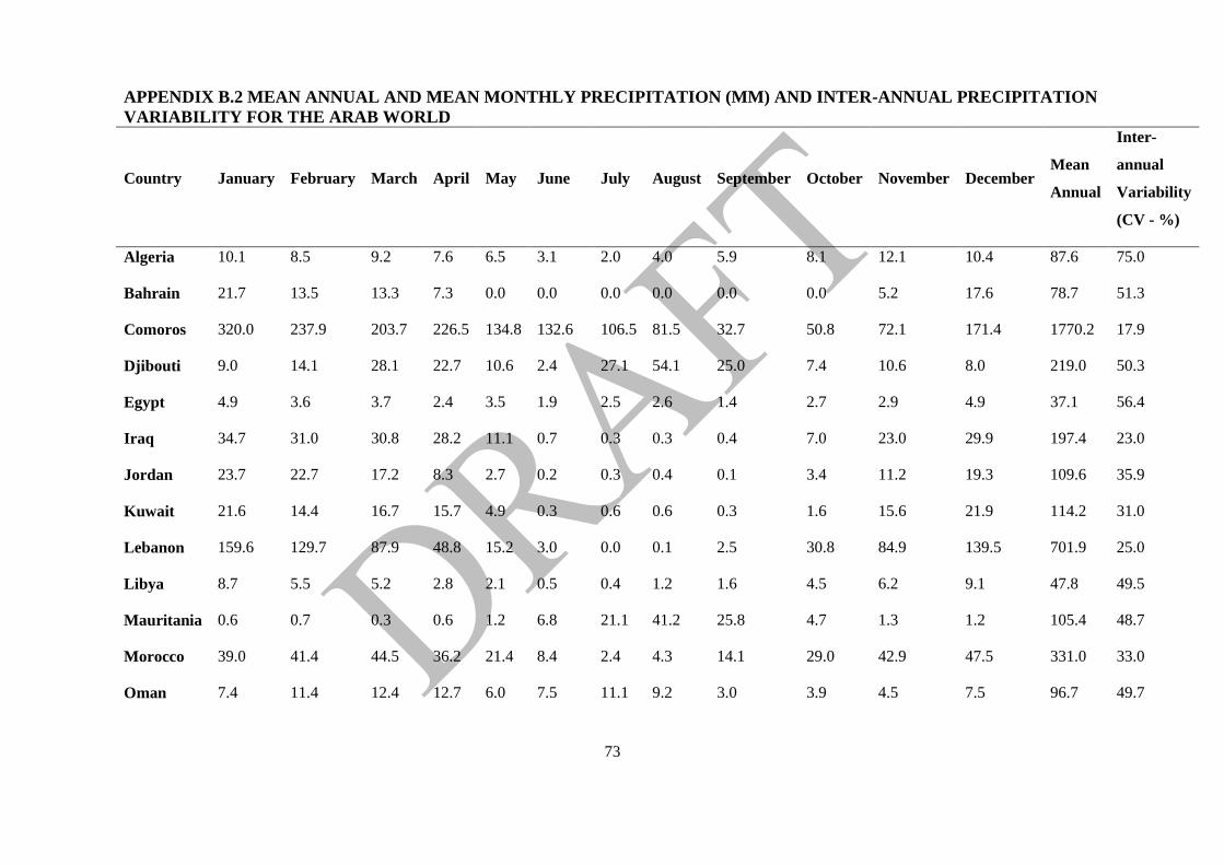
73
APPENDIX B.2 MEAN ANNUAL AND MEAN MONTHLY PRECIPITATION (MM) AND INTER-ANNUAL PRECIPITATION
VARIABILITY FOR THE ARAB WORLD
Country January February March April May June July August September October November December Mean
Annual
Inter-
annual
Variability
(CV - %)
Algeria 10.1 8.5 9.2 7.6 6.5 3.1 2.0 4.0 5.9 8.1 12.1 10.4 87.6 75.0
Bahrain 21.7 13.5 13.3 7.3 0.0 0.0 0.0 0.0 0.0 0.0 5.2 17.6 78.7 51.3
Comoros 320.0 237.9 203.7 226.5 134.8 132.6 106.5 81.5 32.7 50.8 72.1 171.4 1770.2 17.9
Djibouti 9.0 14.1 28.1 22.7 10.6 2.4 27.1 54.1 25.0 7.4 10.6 8.0 219.0 50.3
Egypt 4.9 3.6 3.7 2.4 3.5 1.9 2.5 2.6 1.4 2.7 2.9 4.9 37.1 56.4
Iraq 34.7 31.0 30.8 28.2 11.1 0.7 0.3 0.3 0.4 7.0 23.0 29.9 197.4 23.0
Jordan 23.7 22.7 17.2 8.3 2.7 0.2 0.3 0.4 0.1 3.4 11.2 19.3 109.6 35.9
Kuwait 21.6 14.4 16.7 15.7 4.9 0.3 0.6 0.6 0.3 1.6 15.6 21.9 114.2 31.0
Lebanon 159.6 129.7 87.9 48.8 15.2 3.0 0.0 0.1 2.5 30.8 84.9 139.5 701.9 25.0
Libya 8.7 5.5 5.2 2.8 2.1 0.5 0.4 1.2 1.6 4.5 6.2 9.1 47.8 49.5
Mauritania 0.6 0.7 0.3 0.6 1.2 6.8 21.1 41.2 25.8 4.7 1.3 1.2 105.4 48.7
Morocco 39.0 41.4 44.5 36.2 21.4 8.4 2.4 4.3 14.1 29.0 42.9 47.5 331.0 33.0
Oman 7.4 11.4 12.4 12.7 6.0 7.5 11.1 9.2 3.0 3.9 4.5 7.5 96.7 49.7
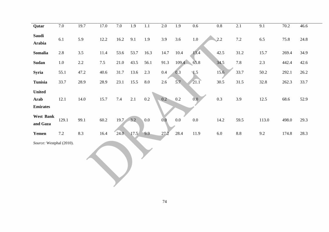
74
Qatar 7.0 19.7 17.0 7.0 1.9 1.1 2.0 1.9 0.6 0.8 2.1 9.1 70.2 46.6
Saudi
Arabia 6.1 5.9 12.2 16.2 9.1 1.9 3.9 3.6 1.0 2.2 7.2 6.5 75.8 24.8
Somalia 2.8 3.5 11.4 53.6 53.7 16.3 14.7 10.4 13.4 42.5 31.2 15.7 269.4 34.9
Sudan 1.0 2.2 7.5 21.0 43.5 56.1 91.3 109.4 65.8 34.5 7.8 2.3 442.4 42.6
Syria 55.1 47.2 40.6 31.7 13.6 2.3 0.4 0.3 1.5 15.6 33.7 50.2 292.1 26.2
Tunisia 33.7 28.9 28.9 23.1 15.5 8.0 2.6 5.7 21.1 30.5 31.5 32.8 262.3 33.7
United
Arab
Emirates
12.1 14.0 15.7 7.4 2.1 0.2 0.2 0.2 0.0 0.3 3.9 12.5 68.6 52.9
West Bank
and Gaza 129.1 99.1 60.2 19.7 3.2 0.0 0.0 0.0 0.0 14.2 59.5 113.0 498.0 29.3
Yemen 7.2 8.3 16.4 24.0 17.5 9.9 27.2 28.4 11.9 6.0 8.8 9.2 174.8 28.3
Source: Westphal (2010).
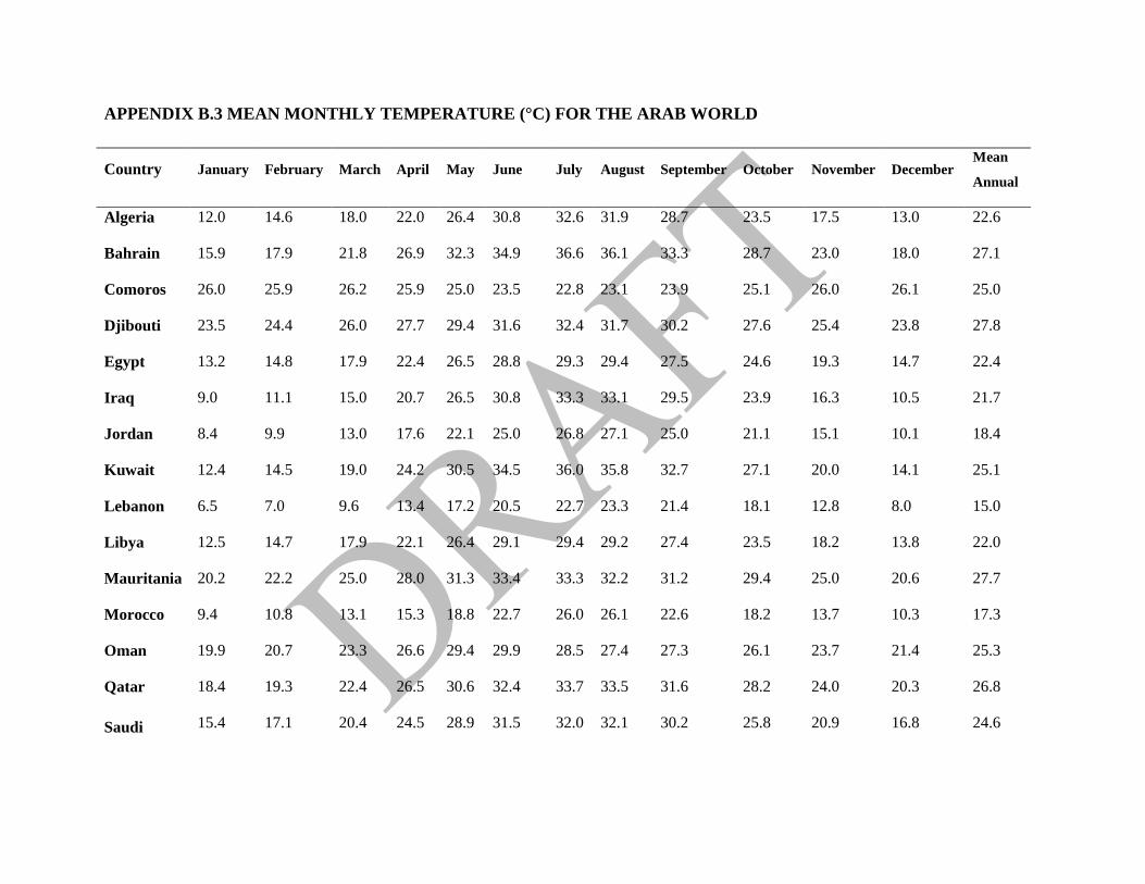
APPENDIX B.3 MEAN MONTHLY TEMPERATURE (°C) FOR THE ARAB WORLD
Country January February March April May June July August September October November December Mean
Annual
Algeria 12.0 14.6 18.0 22.0 26.4 30.8 32.6 31.9 28.7 23.5 17.5 13.0 22.6
Bahrain 15.9 17.9 21.8 26.9 32.3 34.9 36.6 36.1 33.3 28.7 23.0 18.0 27.1
Comoros 26.0 25.9 26.2 25.9 25.0 23.5 22.8 23.1 23.9 25.1 26.0 26.1 25.0
Djibouti 23.5 24.4 26.0 27.7 29.4 31.6 32.4 31.7 30.2 27.6 25.4 23.8 27.8
Egypt 13.2 14.8 17.9 22.4 26.5 28.8 29.3 29.4 27.5 24.6 19.3 14.7 22.4
Iraq 9.0 11.1 15.0 20.7 26.5 30.8 33.3 33.1 29.5 23.9 16.3 10.5 21.7
Jordan 8.4 9.9 13.0 17.6 22.1 25.0 26.8 27.1 25.0 21.1 15.1 10.1 18.4
Kuwait 12.4 14.5 19.0 24.2 30.5 34.5 36.0 35.8 32.7 27.1 20.0 14.1 25.1
Lebanon 6.5 7.0 9.6 13.4 17.2 20.5 22.7 23.3 21.4 18.1 12.8 8.0 15.0
Libya 12.5 14.7 17.9 22.1 26.4 29.1 29.4 29.2 27.4 23.5 18.2 13.8 22.0
Mauritania 20.2 22.2 25.0 28.0 31.3 33.4 33.3 32.2 31.2 29.4 25.0 20.6 27.7
Morocco 9.4 10.8 13.1 15.3 18.8 22.7 26.0 26.1 22.6 18.2 13.7 10.3 17.3
Oman 19.9 20.7 23.3 26.6 29.4 29.9 28.5 27.4 27.3 26.1 23.7 21.4 25.3
Qatar 18.4 19.3 22.4 26.5 30.6 32.4 33.7 33.5 31.6 28.2 24.0 20.3 26.8
Saudi 15.4 17.1 20.4 24.5 28.9 31.5 32.0 32.1 30.2 25.8 20.9 16.8 24.6
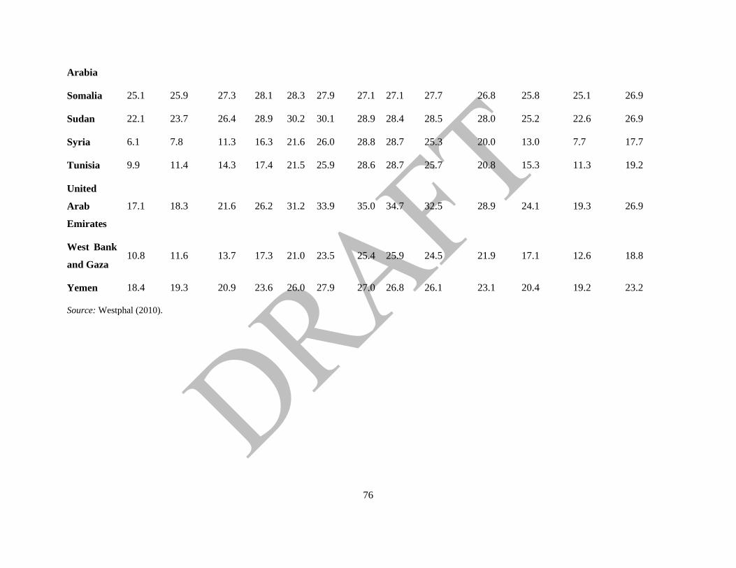
76
Arabia
Somalia 25.1 25.9 27.3 28.1 28.3 27.9 27.1 27.1 27.7 26.8 25.8 25.1 26.9
Sudan 22.1 23.7 26.4 28.9 30.2 30.1 28.9 28.4 28.5 28.0 25.2 22.6 26.9
Syria 6.1 7.8 11.3 16.3 21.6 26.0 28.8 28.7 25.3 20.0 13.0 7.7 17.7
Tunisia 9.9 11.4 14.3 17.4 21.5 25.9 28.6 28.7 25.7 20.8 15.3 11.3 19.2
United
Arab
Emirates
17.1 18.3 21.6 26.2 31.2 33.9 35.0 34.7 32.5 28.9 24.1 19.3 26.9
West Bank
and Gaza 10.8 11.6 13.7 17.3 21.0 23.5 25.4 25.9 24.5 21.9 17.1 12.6 18.8
Yemen 18.4 19.3 20.9 23.6 26.0 27.9 27.0 26.8 26.1 23.1 20.4 19.2 23.2
Source: Westphal (2010).
REFERENCES
Almazroui, M: Sensitivity of a regional climate model on the simulation of high intensity rainfall
events over the Arabian Peninsula and around Jeddah (Saudi Arabia) Theor Appl Climatol
(2011) 104:261–276, DOI: 10.1007/s00704-010-0387-3
Alderwish, A. and El-Eryani, M., 1999: An approach for assessing the vulnerability of the water
resources of Yemen to climate change. Clim. Res. 12, 85-89.
AMAP (2009) The Greenland Ice Sheet in a Changing Climate: Snow, water, ice and permafrost
in the Arctic (SWIPA) Edited by Dahl-Jensen D, Bamber J, Bøggild CE, Buch E, Christensen
JH, Dethloff K, Fahnestock M, Marshall S, Rosing M, Steffen K, Thomas R, Truffer M, van den
Broeke CJ. Arctic Monitoring and Assesment Programme (AMAP), Oslo, 115 pp.
Black, E., 2009: The impact of climate change on daily precipitation statistics in Jordan and
Israel. Atm. Sci. Lett. 10, 192-200, doi: 10.1002/asl.233
Black, E., 2010: Water and society in Jordan and Israel today: an introductory overview. Phil.
Trans. R. Soc. A 368,5111-5116, doi: 10.1098/rsta.2010.0217.
Bonsal, B.R., X. Zhang, L.A. Vincent and W.D. Hogg, 2001: Characteristics of daily and
extreme temperatures over Canada. J. Climate 14, 1959-1976.
Chaponniere, A. and V. Smakhtin, 2006: A review of climate change scenarios and preliminary
rainfall trend analysis in the Oum er Rbia Basin, Morocco. Working Paper 110 (Drought Series:
Paper 8), International Water Management Institute (IWMI), Colombo, Sri Lanka, 16 pp.
Christensen, J.H. and O.B. Christensen, 2003: Severe Summer Flooding in Europe, Nature, 421,
805-806.
Christensen, J.H., B. Hewitson, A. Busuioc, A. Chen, X. Gao, I. Held, R. Jones, R.K. Kolli, W.-
T. Kwon, R. Laprise, V. Magaña Rueda, L. Mearns, C.G. Menéndez, J. Räisänen, A. Rinke, A.
Sarr and P. Whetton, 2007: Regional Climate Projections, Chapter 11 in: Climate Change 2007:
The Physical Science Basis. Contribution of Working Group I to the Fourth Assessment Report
of the Intergovernmental Panel on Climate Change [Solomon, S., D. Qin, M. Manning, Z. Chen,
M. Marquis, K.B. Averyt, M. Tignor and H.L. Miller (eds.)]. Cambridge University Press,
Cambridge, United Kingdom and New York, NY, USA.
Christensen JH, Carter TR, Rummukainen M, Amanatidis G. 2007b. Evaluating the performance
and utility of regional climate models: the PRUDENCE project. Climatic Change 81(Suppl 1):1-
6. DOI:10.1007/s10584-006-9211-6.
Christensen JH, Boberg F, Christensen OB, Lucas-Picher P. 2008: On the need for bias
correction of regional climate change projections of temperature and precipitation. Geophys.
Res. Lett., 35, L20709, doi:10.1029/2008GL035694.
Christensen JH, Rummukainen M. 2009. Choosing ENSEMBLES regional Climate Model
(RCM) simulations and projections for regional climate change and impact analyses. Appendix
for ENSEMBLES deliverable D3.2.2. Available at http://ensembles-eu.metoffice.com/
Christensen JH, Kjellström E, Giorgi F, Lenderink G, Rummukainen M. 2010. Clim. Res. 44,
179-194. doi:10.3354/cr00916.
78
Christensen, O.B. and J.H. Christensen, 2004: Intensification of extreme European summer
precipitation in a warmer climate. Global and Planetary Change, 44, 107-117.
Coppola, E., F. Kucharski, F. Giorgi and F. Molteni, 2005: Bimodality of the North Atlantic
Oscillation in simulations with greenhouse gas forcing. Geophys. Res. Lett. 32, L23709.
Cullen, H.M., A. Kaplan, P.A. Arkin and P.B. de Menocal, 2002: Impact of the NAO on Middle
Eastern climate and streamflow. Clim. Change 55, 315-338.
Dai, A., 2010: Drought under global warming: a review. WIREs Clim. Change 2, 45-65, dooi:
10.1002/wcc81.
Evans, J.P., 2009: 21st century climate change in the Middle East. Clim. Change 92, 417-432,
doi: 10.1007/s10584-008-9438-5.
Evans, J.P., 2010: Global warming impact on the dominant precipitation processes in the Middle
East. Theor. Appl. Climatol. 99, 389-402, doi: 10.1007/s00704-009-0151-8.
Evans, J. and R. Geerken, 2004: Discrimination between climate and human-induced dryland
degradation , J. Arid Environm. 535-554.
Freiwan, M. and M. Kadioglu, 2008a: Climate variability in Jordan. Internat. J. Climatol. 28, 68-
89.
Freiwan, M. and M. Kadioglu, 2008b: Spatial and temporal analysis of climatological data in
Jordan. Internat. J. Climatol. 28, 521-535.
Frich, P., et al., 2002: Observed coherent changes in climatic extremes during the second half of
the twentieth century. Clim. Res., 19, 193–212.
Gao, X.J andF. Giorgi 2008 Increased aridity in the Mediterranean region under greenhouse gas
forcing estimated from high resolution simulations with a regional climate model Global and
Planetary Change 62 3-4 195-209
Giorgi, F., C. Jones, and G. R. Asrar, 2009: Addressing climate information needs at the regional
level: The CORDEX framework. WMO Bull., 58, 175–183.
Haylock, M.R., N. Hofstra, A.M.G. Klein Tank, E.J. Klok, P.D: Jones and M. New, 2008: A
European daily high-resolution gridded data set of surface temperature and precipitation for
1950-2006. J. Geoph. Res. 113, D20119
Hurrell, J., T. Delworth, G. Danabasoglu, H. Drange,K. Drinkwater, S. Griffies, N.Holbrook, B.
Kirtman, N. Keenlyside,M. Latif, J. Marotzke, J. Murphy,G. Meehl, T. Palmer, H. Pohlmann, T.
Rosati, R. Seager, D. Smith, R. Sutton, A. Timmermann, K. Trenberth,J. Tribbia, and M.
Visbeck, 2010: Decadal Climate Prediction: Opportunities and Challenges in Proceedings of
OceanObs‘09: Sustained Ocean Observations and Information for Society (Vol. 2), Venice, Italy,
21-25 September 2009, Hall, J., Harrison, D.E. & Stammer, D., Eds., ESA Publication WPP-306,
doi:10.5270/OceanObs09.cwp.45.
IPCC, 2007: Summary for Poicymakers. In: Climate Change 2007: The Physical Science Basis.
Contribution of Working Group I to the Fourth Assessment Report of the Intergovernmental
Panel on Climate Change [Solomon, S., D. Qin, M. Manning, Z. Chen, M. Marquis, K.B.
79
Averyt, M.Tignor and H.L. Miller (eds.)]. Cambridge University Press, Cambridge, United
Kingdom and New York, NY, USA.
IOP, 2009: Climate Change: Global Risks, Challenges and Decisions, Copenhagen 10.-12.
March 2009. All sessions. IOP Conference Series: Earth and Environmental Series. Available
online at: http://www.iop.org/EJ/volume/1755-1315/6.
Johns, T.C, J.-F. Royer, I. Ho¨schel, H. Huebener, E. Roeckner, E. Manzini, W. May, J.-L.
Dufresne, O. H. Ottera°, D. P. van Vuuren, D. Salas y Melia, M. A. Giorgetta, S. Denvil, S.
Yang, P. G. Fogli, J. Körper, J. F. Tjiputra, E. Stehfest, C. D. Hewitt, 2011: Climate change
under aggressive mitigation: the ENSEMBLES multi-model experiment. Clim Dyn., DOI
10.1007/s00382-011-1005-5.
Kim, D.-W. and H.R. Byun, 2009: Future patterns of Asian drought under global warming
scenario. Theor. Appl. Climatol. 98, 138-150.
Kitoh, A., A. Yatagai and P. Alpert, 2008: First super-high resolution model projection that the
ancient ―Fertile Crescent‖ will disappear in this century. Hydrol. Res. Lett. 2, 1-4.
Kjellström E, Giorgi F. 2010. Introduction. Clim Res 44:117-119.
Knippertz, P., 2003: Tropical-extratropical interactions causing precipitation in Northwest
Africa: Statistical analysis and seasonal variations. Mon. Wea. Rev. 131, 3069-2076
Knippertz, P., 2004: A simple identification scheme for upper-level troughs and its application to
winter precipitation variability in Northwest Africa. J. Climate 17, 1411-1418
Knippertz, P., M. Christoph and P. Speth, 2003: Long-term precipitation variability in Morocco
and the link to the large-scale circulation in recent and future climates. Meteorol. Atmosph. Phys.
83, 67-88.
Krichak, S.O., P. Alpert and P. Kunin, 2010: Numerical simulation of seasonal distribution of
precipitation over the eastern Mediterranean with a RCM. Clim. Dyn. 34, 47-59.
Kummerow, C., et al., 2000. The status of the Tropical Rainfall Measuring Mission (TRMM)
after two years in orbit. J. Appl.Meteorol. 39, 1965–1982.
Latif, M., T. Delworth, D. Dommenget, H. Drange, W. Hazeleger, J. Hurrell, N. Keenlyside, G.
Meehl and R. Sutton, 2010: Dynamics of Decadal Climate Variability and Implications for its
Prediction in Proceedings of OceanObs‘09: Sustained Ocean Observations and Information for
Society (Vol. 2), Venice, Italy, 21-25 September 2009, Hall, J., Harrison, D.E. & Stammer, D.,
Eds., ESA Publication WPP-306, doi:10.5270/OceanObs09.cwp.53
Lionello, P. and F. Georgi, 2007: Winter precipitation and cyclones in the Mediterranean region:
future climate scenarios in a regional simulation. Adv. Geoscience 12, 153-158.
Mahwed, K., 2008: Vulnerability assessment of the climate sector. Enabling activities for
preparation of Syria‘s initial communication to the UNFCCC (Project no. 00045323), 47 pp.
Mearns, LO, Hulme M, Carter TR., Leemans R, Lal M, Whetton P, Hay L, Jones RN, Katz R,
Kittel T, Smith J, Wilby R, Mata, LJ, Zillman J. 2001: Climate Scenario Development. In
Climate Change 2001: The Scientific Basis. Contribution of Working Group I to the Third
Assessment Report of the Intergovernmental Panel on Climate Change [Houghton JT, Ding Y,
80
Griggs DJ, Noguer M, van der Linden PJ, Dai X, Maskell K, Johnson CA (eds.)]. Cambridge
University Press, Cambridge, United Kingdom and New York, NY, USA, 881 pp.
Meehl, G.A., T.F. Stocker, W.D. Collins, P. Friedlingstein, A.T. Gaye, J.M. Gregory, A. Kitoh,
R. Knutti, J.M. Murphy, A. Noda, S.C.B. Raper,I.G. Watterson, A.J. Weaver and Z.-C. Zhao,
2007: Global Climate Projections. In: Climate Change 2007: The Physical Science Basis.
Contribution of Working Group I to the Fourth Assessment Report of the Intergovernmental
Panel on Climate Change [Solomon, S.,D. Qin, M. Manning, Z. Chen, M. Marquis, K.B. Averyt,
M. Tignor and H.L. Miller (eds.)]. Cambridge University Press, Cambridge, United Kingdom
and New York, NY, USA.
Meehl, G. A., L. Goddard, J. Murphy, R. J. Stouffer, G. Boer, G. Danabasoglu, K. Dixon, M. A.
Giorgetta, A. Greene, E. Hawkins, G. Hegerl, D. Karoly, N. Keenlyside, M. Kimoto, B. Kirtman,
A. Navarra, R. Pulwarty, D. Smith, D. Stammer, and T. Stockdale (2009): Decadal prediction:
Can it be skillful? Bull. Amer. Meteorol. Soc., DOI:15 10.1175/2009BAMS2778.1.
Moss RH, Babiker M, Brinkman S, Calvo E, Carter T, Edmonds J, Elgizouli I, Emori S, Erda L,
Hibbard K, Jones R, Kainuma M, Kelleher J, Lamarque JF, Manning M, Matthews B, Meehl G,
Meyer L, Mitchell J, Nakicenovic N, O‘Neill B, Pichs T, Riahi K, Rose S, Runci P, Stouffer R,
van Vuuren D, Weyant JW, T., van Ypersele JP, Zurek M, 2008: Towards New Scenarios for
Analysis of Emissions, Climate Change, Impacts, and Response Strategies. Intergovernmental
Panel on Climate Change, Geneva.
Moss RH, Edmonds JA, Hibbard KA, Manning MR, Rose SK, van Vuuren DP, Carter TR,
Emori S, Kainuma M, Kram T, Meehl GA, Mitchell JFB, Nakicenovic N, Riahi K, Smith SJ,
Stouffer RJ, Thomson AM, Weyant JP, Wilbanks TJ, 2010: The next generation of scenarios for
climate change research and assessment. Nature 463:747-756.
Mote, T.L.,2007: Greenland surface melt trends 1973 – 2007: Evidence of a large increase in
2007, Geophys. Res. Lett., 34, L22507, doi: 10.1029/2007GL031976.
Murphy, J., Kattsov, V., Keenlyside, N., Kimoto, M., Meehl, G., Mehta, V., Pohlmann, H.,
Scaife, A., and Smith, D., 2010: Towards Prediction of Decadal Climate Variability and Change.
Procedia Environmental Sciences, 1, 287-56 304, doi:10.1016/j.proenv.2010.09.018.
Nasrallah, H.A. and R.C. Balling, 1993: Spatial and temporal analysis of Middle-Eastern
temperature changes. Clim. Change 25, 153-161.
Olesen JE, Carter TR, Diaz-Ambrona CH, Fronzek S, Heidmann T, Hickler T , Holt T, Minguez
MI, Morales P, Palutikof J, Quemada M, Ruiz-Ramos M, Rubæk G, Sau F, Smith B, Sykes M.
2007. Uncertainties in projected impacts of climate change on European agriculture and
ecosystems based on scenarios from regional climate models. Climatic Change 81, Suppl. 1,
123-143.
Önol, B. and F.H.M. Semazzi, 2009: Regionalization of climate change simulations over the
Eastern Mediterranean. J. Climate 22, 1944-1961
Oroud, I.M., 2008: The impacts of climate change on waterresources in Jordan. In: Zereini, F.
and H. Hotzl (eds.): Climatic changes and water resources in the Middle East and North Africa,
Springer, New York.
81
Raible, C.C., B. Ziv, H. Saaroni and M. Wild, 2010: Winter synoptic-scale variability over the
Mediterranean Basin under future climate conditions as simulated by the ECHAM5. Clim. Dyn.
35, 473-488.
Racsko P, Szeidl L, Semenov M. 1991. A serial approach to local stochastic weather models.E
col. Model, 57:27-41.
Rauthe, M., A. Hense and H. Paeth, 2004: A model intercomparison study of climate change
signals in extratropical circulation. Global and Environmental Change – Human and Policy
Dimensions 9, 45-58.
Reifen C, Toumi R. 2009. Geophys. Res. Letters 36, L13704, 10 doi:10.1029/2009GL038082.
Rummukainen M. 2010. State-of-the-art with regional climate models. Wiley Interdisciplinary
Reviews: Climate Change, 1:82–96. doi:10.1002/wcc.8.
Schneider U, Fuchs T, Meyer-Christoffer A, Rudolf B (2008) Global precipitation analysis
products of the GPCC. Global Precipitation Climatology Centre (GPCC), DWD, Internet
Publikation, 1–12.
Semenov MA, Brooks RJ, Barrow EM, Richardson CW. 1998. Comparison of the WGEN and
LARS-WG stochastic weather generators for diverse climates. Climate Research 10, 95-107
Sensoy, S., T.C. Peterson, L.V. Alexander and Z. Xuebin, 2007: Enhancing Middle East climate
change monitoring and indexes. Bull. Amer. Met. Soc. 88, 1249-1254.
Shahin, M., 2007: Water resources and hydrometeorology of the Arab region. Water Science and
Technology Library, vol. 59, Springer, The Netherlands, 586 pp.
Simpson, J., Adler, R.F., North, G.R., 1988. A proposed Tropical Rainfall Measuring Mission
(TRMM) satellite. Bull. Am. Meteorol. Soc. 69, 278–295.
Smadi, M.M. and A. Zghoul, 2006: A sudden change in rainfall characteristics in Amman,
Jordan during the mid-1950s. Amer. J. Environm. Changes 2, 84-91.
Sowers, J., A. Vengosh and E. Weinthal, 2011: Climate change, water resources and the politics
of adaptation in the Middle East and North Africa. Clim. Change 104, 599-627, doi:
10.1007/s10584-010-9835-4.
Steffen, K., and Huff, R.,2009: University of Colorado at Boulder, personal communication.
Taylor, K.E.,R.J. Stouffer, G.A. Meehl, 2011: A Summary of the CMIP5 Experiment Design.
(Available from http://cmip-pcmdi.llnl.gov/cmip5/).
Tebaldi, C., K. Hayhoe, J.M. Arblaster, and G.A. Meehl, 2006: Going to the extremes: An
intercomparison of model-simulated historical and future changes in extreme events. Clim.
Change, 79, 185-211
Tryhorn, L., A. Lynch, and R. Abramson, 2008: On the meteorological mechanisms driving
postfire flash floods: A case study. Monthly Weather Review, 136, 1778-1791.
Tschoegl, L., R. Below, Guhar-Sapir, D. 2006: An Analytical Review of Selected Data Sets on
Natural Disasters and Impacts. Centre for Research on the Epidemiology of Disasters (CRED),
Université catholique de Louvain, Belgium. (Available at http://www.em-
dat.net/documents/Publication/TschoeglDataSetsReview.pdf).
82
Van den Brink, H.W., G.P. Konnen, J.D. Opsteegh, G.J. Van Oldenborgh, and G. Burgers, 2005:
Estimating return periods of extreme events from ECMWF seasonal forecast ensembles.
International Journal of Climatology, 25(10), 1345-1354.
van der Linden P, Mitchell JFB (eds) (2009) ENSEMBLES: climate change and its impacts.
Summary of research and results from the ENSEMBLES project. Met Office Hadley Centre,
Exeter.
van Vuuren, D., K. Riahi, R.H. Moss, J. Edmonds, A. Thomson, N. Nakicenovic, T. Kram, F.
Berkhout, R. Swart, A. Janetos, S. Rose and N. Arnell, 2010: Developing new scenarios as a
common thread for future climate research. (Available from http://www.ipcc-
wg3.de/meetings/expert-meetings-and-workshops/files/Vuuren-et-al-2010-Developing-New-
Scenarios-2010-10-20.pdf/view?searchterm=New%20Scenarios).
Westphal, MI (2010) The Arab World historical climate and future climate projections, WB
background paper.
Wilby, R.L., 2007: Climate change scenarios for Morocco. Final Technical Report, WB
background paper.
Wilby, R.L., 2008: Climate change scenarios for the Republic of Yemen. Revised Technical
Report, WB background paper.
Wilby, R.L., 2010: Climate change projections and downscaling for Jordan, Lebanon and Syria.
Draft Synthesis Report, WB background paper.
Wilby, R.L., J. Troni, Y. Biot, L. Tedd, B.C. Hewitson, D.M. Smith and R.T.Sutton, 2008: A
review of climate risk information for adaptation and development planning. Int. J. Climatology
29, 1193-1215.
Yatagai, A., P. Xie and P. Alpert (2008): Development of a daily gridded precipitation data set
for the Middle East, Adv.in Geosci. 12, 165-170.
Zhang, X., E. Aguilar, S. Sensoy, H. Melkonyan, U. Tagiyeva, N. Ahmed, N. Kutaladze, F.
Rahimzadeh, A. Taghipour, T.H. Hantosh, P. Alpert, M. Semawi, M.K. Ali, M.H.S. Al-Shabibi,
Z. Al-Oulan, T Zatari, I. Al Dean Khelet, S. Hamoud, R. Sagir, M. Demircan, M. Eken, M.
Adiguzel, L. Alexander, T.C. Peterson and T. Wallis, 2005: Trends in Middle East climate
extreme indices from 1950 to 2003. J. Geophys. Res. 110, D22104, doi:10.1029/2005JD006181.