48

CHAPTER 2

TRANSIENT STABILITY OF SMIB SYSTEM USING

NONLINEAR CONTROL TECHNIQUE

2.1 INTRODUCTION

Electrical power systems play a vital role in modern human life and

any disturbances in their normal functioning cause interruptions to both the

component and system level. A large power system is very complex and

consists of various components such as power generating units which are

connected to each other and with distributed loads through very long

transmission lines, transformers and capacitors. The power system is a highly

nonlinear in nature. One of the most important aspects in electric system

operation is the stability of power systems. The property of the system to

return to an acceptable working condition following a transient is called the

transient stability and it is a critical issue in power systems. Typically systems

are lightly damped and are prone to heavy sustained oscillations after a

transient. Moreover, their nonlinear nature makes them difficult to control.

Control of power swing oscillations is an important control problem.

An important factor, which decides the capacity of a transmission

line to transfer the electrical power across the network, is the reactance of the

transmission line which decides the stability margin of the power system.

Many power electronic devices have been invented for increasing the capacity

and stability margin of the power systems. The concept of Flexible AC

Transmission System (FACTS) realized by Ghandhari et al (2001), Banaei &

49

Gholizadeh (2011) relies on the use of power electronic devices, and offers

greater control of power flow, secure loading and damping of power system

oscillations. These devices can be classified into two categories, one is shunt

devices in which the injected current is controlled, and the other is series

devices in which the inserted voltages are controlled. Static Var Compensator

(SVC) is an example of shunt devices, while series devices include Unified

Power Flow Controller (UPFC), Controllable Series Capacitor (CSC)

(Hemeida et al 2010).

Conventionally linear controllers are used to stabilize the power

system. In linear controllers, initially, the system is linearised about an

equilibrium point. Then design the controller for the linear system. In that

case the corresponding linear controller may not be adequate to stabilize the

system. There are two basic limitations of linearization. Firstly, it can only

predict the local behaviour of the nonlinear systems. And it cannot predict the

non local behaviour far from the operating point. Secondly the dynamics of

the nonlinear systems are much richer than the dynamics of a linear system.

Since there are nonlinear phenomena that can take place only in the presence

of nonlinearities like finite escape time, multiple isolated equilibrium point,

limit cycles, harmonic oscillations, chaos, etc. which cannot be described and

predicted by linear models.

Recently the application of nonlinear control theory like excitation

control, feedback linearization and passivity based control techniques has

been investigated for improving the transient stability of a power system.

Nonlinear control using turbine control, excitation control law, and feedback

linearization were applied to the single as well as multi machine systems, as

proposed by Lu & Sun (1989), King et al (1994), Ortega et al (1998),

Li (2006). However, those methods were fragile as it relies on nonlinearity

cancellation, and the issue of robustness remains unanswered, and this

50

motivates for investigation of energy based control of nonlinear systems. This

work addresses the problem of transient stabilization of the Single Machine

Infinite Bus (SMIB) system using Controllable Series Capacitor (CSC).

The organization of the chapter is as follows: Section 2.2 describes

the overview of the proposed method for enhancing the stability of the

system. Section 2.3 discusses the control strategy and section 2.4 discusses

the Immersion and Invariance techniques. The controller synthesis for the

development of control law is described in section 2.5. The improvement in

the stability of the system is illustrated in section 2.6 followed by conclusion

in section 2.7.

2.2 PROBLEM DEFINITION

The stability problem arises from the fact that for the system under

normal conditions, the average electrical speed of the generators must remain

the same anywhere in the system. This is termed as synchronous operation of

a system. Any small or large disturbances can affect the synchronous

operation (Hadi Saddat 2002). Recently the application of nonlinear control

techniques with Flexible AC Transmission Systems (FACTS) has been

investigated for improving transient stability of power systems. FACTS

technology is often most economic alternative for solving transmission

loading problems. It provides a mechanism to make the best use of existing

transmission. FACTS devices are capable of acting sufficiently to improve all

forms of stability as well as steady state conditions. Advancements in power

electronics has revolutionized the design and engineering concepts of the

FACTS devices. FACTS devices are highly effective in both controlling

power flow and in improving stability. This work uses a nonlinear control

technique called Immersion and Invariance (I&I) which uses CSC as an

actuator, which is connected in series with the transmission line. The control

system consisting of two subsystems, namely the second order nonlinear

51

swing equation of the SMIB system, and a first order system representing the

CSC have been explained by Manjarekar et al (2008). Astolfi & Ortega

(2003) proposed the Immersion and Invariance control strategy to achieve the

control objective. The SMIB stabilization is achieved using energy shaping

and damping assignment for the system.

2.3 CONTROL STRATEGY

The SMIB system with CSC proposed by Manjarekar et al (2008)

is shown in Figure 2.1. In practice, an infinite bus is a large power system

with a large inertia. Such a system does not exhibit significant oscillations on

the occurrence of transients and is considered as a reference bus to assess the

performance of a synchronous generator connected to it. The infinite bus is

denoted by bus 2 and the generator internal bus is connected to the infinite

bus through the transient reactance . The controllable series capacitor is

represented by variable capacitor .

Figure 2.1 SMIB system with CSC

where

is the rotor angle

E denotes the constant voltage behind the transient reactance of the

generator.

is direct axis transient reactance of the generator

VE21 djx'

cjx

G

52

The proposed work develops a nonlinear control law to

asymptotically stabilize SMIB system based on immersion and invariance

control strategy. The actuator used is a controllable series capacitor. The

control system considered has two subsystems, the second order nonlinear

swing equation of the SMIB system, and a first order system representing the

CSC. The control synthesis is based on two important nonlinear tools:

immersion (system) and invariance (manifold). The control objective is to

approximate the complete third order system with a second order dynamics,

for which an asymptotically stabilizing control law is proposed. The proposed

control law includes the damping factor which quickly damps out the power

system oscillations caused by interruptions. During an unstable condition, the

declining rate of the power system oscillation is determined by the damping

factor in the power system. The SMIB system stabilization is achieved using

energy shaping and damping of electromechanical oscillations in the system.

Let D be the damping constant (D > 0)

M be the moment of inertia constant (M > 0) and

P be the mechanical power input

Here the effect of saliency of the rotor is neglected. Also is

constant and is assumed to be zero. Let the effective line reactance between

bus1 and bus 2 be denoted by and the few assumptions are considered as

given in Equation (2.1).

The region of operation is

(2.1)

where are small numbers.

53

2.3.1 System Model

First the SMIB system described by Manjarekar et al (2008) using

the swing equation model is given in Equations (2.2) and (2.3).

(2.2)

The actuator is represented by using a first order equation of the form

(2.3)

where Tcsc is the time constant of the actuator, is the line reactance at the

desired equilibrium point and u is the input to the actuator. The state variables

of the system are defined as

And is a state vector T

The open loop operating equilibrium is denoted by The

complete control system can be represented using Equations (2.4) and (2.5),

(2.4)

54

or equivalently,

(2.5)

where for a given

2.3.2 Control Objective

In Equation (2.1), denotes the known operating equilibrium

point, and the control objective is stated as to design a control law u in order

to make the system represented in Equation (2.4) to be asymptotically

stable at .

2.4 IMMERSION AND INVARIANCE METHOD

The concept of invariance has been widely used in control theory.

For stabilization and for analysis of slow adaption systems slow and fast

invariant manifolds are used. Recently Astolfi & Ortega (2003) have

discovered that the notion of invariant manifolds is crucial in the design of

stabilizing control laws for classes of nonlinear systems. In this work

Immersion and Invariance (I&I) method is employed to design stabilizing and

adaptive control laws.

Main features of immersion and invariance method are:

Invariance: Invariant subspaces, invariant distributions play a

fundamental role in the design.

55

Immersion: To project the system under consideration into a

system with prescribed properties.

Immerse a generic non linear system into a linear and

controllable one by means of static and dynamic state

feedback system.

Does not require the knowledge of construction of a

Lyapunov function.

In the controller design, the complete third order system is

immersed in a reduced order target dynamics which is of order two. Astolfi &

Ortega (2003), Manjarekar et al (2008), Ghandhari et al (2001), Hoseynpoor

et al (2011) explained that the restriction of the full order system dynamics

coincides with the target dynamics by constructing manifold.

2.5 CONTROLLER DESIGN USING I&I

The state space model of the system is given in Equation (2.6)

(2.6)

where and are smooth functions, with state and control

, with an equilibrium point to be stabilized. Let p < n and

assume the following mappings,

Such that the following conditions hold as given in Equations (2.7),

(2.8), (2.9), (2.10), (2.11) and (2.12).

56

The system (Target System H1)

(2.7)

With state has an asymptotically stable equilibrium at

and

Immersion condition (H2) for all

(2.8)

Implicit manifold (H3)

The following set identity holds

(2.9)

Manifold attractivity and trajectory boundedness (H4)

All trajectories of the system

(2.10)

(2.11)

are bounded and satisfy

(2.12)

where and . Then x is an asymptotically stable

equilibrium of the closed loop system

57

The Equation (2.6) interpreted as theorem 1 for a given system and

for the target dynamics of the system as given in Equation (2.7), the manifold

M can be rendered as invariant and attractive.

2.6 CONTROLLER SYNTHESIS USING I&I

The control synthesis is based on two important nonlinear tools:

system (immersion) and manifold (invariance). The complete third order

system is immersed in a reduced order target dynamics of order two. The

target system is asymptotically stable. An invariant manifold is constructed

such that the restriction of the full order system dynamics coincides with the

target dynamics.

2.6.1 Target System

However, due to poor damping of open loop system, the transient

response is not satisfactory. Selection of the target dynamics in which the

closed loop system is immersed is a nontrivial task as described by

Hoseynpoor et al (2011). The first step in control synthesis is defined as two

dimensional dynamical system as follows:

Let be the state of the dynamical system

where denotes the potential energy of the system and is possibly

nonlinear damping function. The target system given in Equation (2.13) is a

58

simple pendulum system with a stable equilibrium with the

energy function as given in Equation (2.14),

(2.14)

2.6.2 Immersion Condition

After defining desired target dynamics, the immersion condition as

in Equation (2.8) becomes changed as shown in Equation (2.15)

Next, choose and in order to satisfy (2.15). The first

row of the equation is already satisfied. Then the second row of (2.15)

becomes

By choosing , and for some

> 0, Then Equation (2.15a) becomes

59

Equation (2.15b) indicates that is a function of both and .

To make bounded in a domain of operation and to ensure the stability

at equilibrium, the assumptions are considered as given in Equations (2.16)

and (2.17),

(2.16)

With the assumption given in Equation (2.17), it is realized that

bounded for all . So, the third row of Equation (2.15) becomes

By substituting for and in (2.18), is given in

Equation (2.19).

Thus and are obtained.

2.6.3 Implicit Manifold

The manifold is implicitly described by Equation (2.20)

60

with

where denotes

2.6.4 Manifold Attractivity and Trajectory Boundedness

Off-the manifold coordinate is and having the Equation (2. 21)

(2.22)

is asymptotically stable when the equilibrium of closed loop system when

2.6.5 Control Law

The control law is found,

61

Finally the boundedness of the trajectories of the closed loop

system referred in Equation (2.5) with the control law as given in Equation

(2.23) and the off-the-manifold coordinate z are established. It is found that

the assumption as given in Equation (2.17), is bounded for all , and

hence the closed loop system with control law is asymptotically stable at

2.7 SIMULATION RESULTS

The performance of the controller is assessed for the following two

different transient conditions:

A short circuit fault occurs on the far end of the transmission

line at time t = 20 sec for a duration of about 0.1 sec.

An open circuit fault occurs on one of two parallel transmission

lines at time t = 60 sec for a duration of about 0.1 sec.

The standard simulation parameters considered are (Ghandhari et al

2001), M .

62

, and are considered as tuning parameters. Line reactances are assumed

as constant parameters for the system. To assesses the performance of the

control law, the short circuit fault (L-G) occurs at the far end of the

transmission line at t = 20 sec for a duration of 0.1 sec and an open circuit

fault occurs on one of the two transmission lines at time t = 60 sec for a

duration of about 0.1 sec.

For the short circuit fault, the magnitude of the oscillations is

greater as compared to the open circuit fault. The open loop performances for

rotor angle and rotor angular speed are presented for both the transients as

shown in Figure 2.2. Therefore, additional damping term in the target

dynamics improves the transient performance. Closed loop performances

without damping coefficient assessed for various values of and are shown

in Figure 2.3 to Figure 2.5.

The tuning parameter decides the shape of the energy function of

the closed loop system and decides the rate at which the closed loop system

trajectories reach the desired trajectories. Figure 2.3 shows simulation results

for and . In this case as compared to open loop response the

amplitude of oscillations in rotor angle and rotor angular velocity are very

small. Similarly as in open loop response the oscillations are greater during

short circuit fault than the open circuit fault. But unlike the open loop

response, the line reactance of the system varies with the same magnitude for

both the faults.

63

Figure 2.2 Open loop response

64

Figure 2.3 Closed loop response with and

In the second case, by assuming and , the effect of

increase in is realized. The simulation result plotted in Figure 2.4 shows

improvement in the closed loop response with less magnitude, however, it is

oscillatory in nature. The swing angle experiences rapid oscillations as

compared to the first case, and is further reflected in the response of the

angular velocity. From the plot it has been observed that, increase in

introduces oscillations in the load angle and in the angular velocity.

65

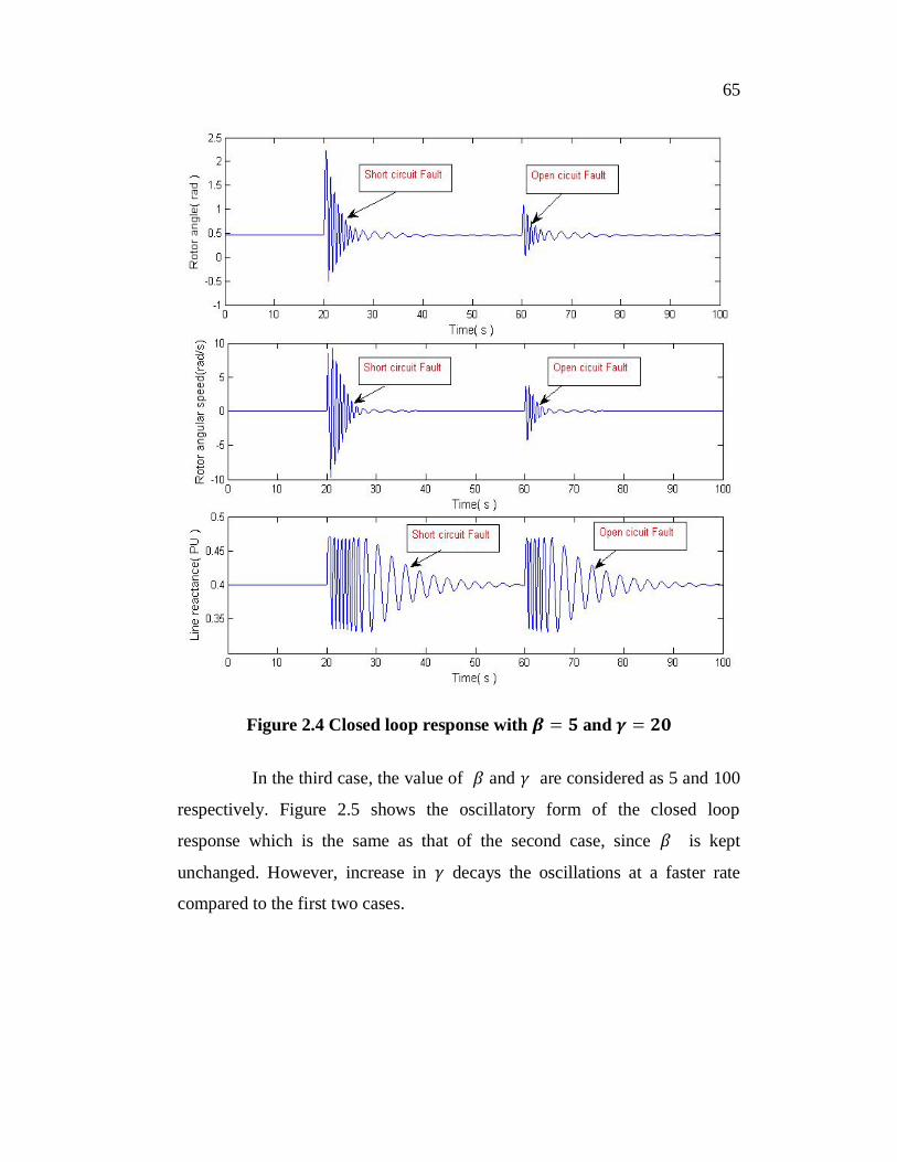
Figure 2.4 Closed loop response with and

In the third case, the value of and are considered as 5 and 100

respectively. Figure 2.5 shows the oscillatory form of the closed loop

response which is the same as that of the second case, since is kept

unchanged. However, increase in decays the oscillations at a faster rate

compared to the first two cases.

66

Figure 2.5 Closed loop response with and

Figure 2.6 shows the closed loop performance for = 30 and

= 50. It has been observed that, there is an improvement in the closed loop

response with fewer oscillations compared to first three cases for both short

circuit and open circuit faults.

67

Figure 2.6 Closed loop response with and

The closed loop performance of the controller without damping

coefficient for various values of and produce the rapid oscillations,

but faster decay of oscillations are not obtained as explained by Manjarekar et

al (2008). Hence, to obtain faster decay of oscillations, the control law with

damping coefficient is considered and the corresponding closed loop

68

performances are shown in Figure 2.7, Figure 2.8 and Figure 2.9 respectively.

From Figure 2.7 for = 5, and = 2.7, it is found that the closed

loop response of the system has reduced oscillations with less magnitude as

compared to closed loop performance without damping coefficient.

Figure 2.7 Closed loop response with and

69

Figure 2.8 Closed loop response with and

70

Figure 2.9 Closed loop response with and

71

From Figure 2.8 and Figure 2.9, it has been observed that the

oscillatory form of the closed loop performance remains the same as that of

the Figure 2.7, since the has not been changed. However, oscillations

decay much faster as compared to previous cases. The tuning parameter

tunes the system, so that the faster decay of oscillations is achieved in rotor

angle and angular velocity, so the transient stability has been improved.

2.8 SUMMARY

In this research work a nonlinear control law is designed to

asymptotically stabilize the SMIB system at equilibrium point based on

immersion and invariance control strategy. The SMIB system is described as

a swing equation model. And the CSC, which is used as an actuator is

described as a first order model. A simple pendulum system with a suitable

energy function was chosen as the target dynamics. The manifold is chosen in

such a way that the closed loop system is restricted to the target dynamics.

The control law has been synthesized in order to render the manifold

invariant. As evident from the graphs, it is clear that the proposed control law

exhibits improved transient performance and reduces the oscillations quickly

compared to existing control law without damping assignment suggested by

Manjarekar et al (2008). Thus the described control technique with damping

assignment exhibits faster decay of oscillations in rotor angle and angular

velocity for various values of tuning parameters.