chapter 16 nonparametric tests - wordpress.com. wilcoxon two-sample test 499 16.1 wilcoxon...

Chapter 16

Nonparametric Tests

The statistical tests we have examined so far are called parametric tests,because they assume the data have a known distribution, such as the normal,and test hypotheses about the parameters of this distribution. Examplesof such tests are the F test in ANOVA, and one- or two-sample t tests.Parametric tests can also be constructed for other distributions, such as thePoisson and binomial.

While ANOVA and other procedures are derived assuming the data arenormal, they can also be validly applied to non-normal data provided samplesizes are large, due to the central limit theorem (Glass et al. 1972). Forexample, the means used in the ANOVA F tests are assumed to have anormal distribution, which will be true for normal data. This will also holdfor non-normal data, provided the sample sizes are sufficiently large for thecentral limit theorem to operate (Chapter 7). Thus, the tests used in ANOVAwill still be valid for large sample sizes, regardless of the distribution of thedata. Valid in this context means the tests have the correct Type I error rate(such as α = 0.05) and power levels.

There are conditions where parametric procedures are less than ideal.For example, suppose that the data appear non-normal and sample sizes arerelatively small. We cannot rely on the central limit theorem here, and soparametric tests based on the normal distribution might be invalid. Non-parametric tests are often useful in this situation. These procedures donot assume a particular probability distribution for the data, and are there-fore applicable for any distribution. For this reason they are also knownas distribution-free methods. Nonparametric tests can be more powerfulthan parametric tests for non-normal data (Conover 1999; Hollander et al.

495

496 CHAPTER 16. NONPARAMETRIC TESTS

2014). The increase in power can be substantial for distributions with heavytails compared to the normal distribution, which implies that extreme obser-vations are more common. While nonparametric tests are less powerful thanparametric ones for normal data, the loss of power is often quite minimal.

We will examine three types of nonparametric tests for one-way designs.The first are tests based on ranks. These replace the data values with theirrank values, obtained by ordering the data from smallest to largest. Theythen utilize test statistics that are functions of these ranks rather than theoriginal data values. We will cover rank tests for two or more groups, inparticular the Wilcoxon and Kruskal-Wallis tests (Conover 1999; Hollanderet al. 2014). They are used to test whether the distributions for each groupdiffer in location, and serve a function similar to parametric tests like one-way ANOVA. We will also examine the two-sample Kolmogorov-Smirnovtest, which can detect differences in both the shape and location of twodistributions (Conover 1999; Hollander et al. 2014). It makes use of theempirical distribution function for each group, the empirical counterpart ofthe distribution function for continuous random variables (Chapter 6). Thelast type of nonparametric test we will consider are randomization tests.These tests examine whether the data are consistent with a null hypothesis ofrandomness (Hinkelmann & Kempthorne 1994; Manly 1997). The behaviorof a test statistic (often a parametric one like an F statistic) is examinedunder this null hypothesis, in a process that involves randomly permuting orrearranging observations across the groups many times.

We will use data from a study of chitons (a kind of mollusk) in the inter-tidal zone (Flores-Campana et al. 2012) to illustrate the use of nonparametrictests. Populations of Chiton albolineatus were sampled from three islands inMazatlan Bay, Mexico. For each island, samples were taken from sites thatwere exposed or sheltered from wave action, and the body length of the chi-tons measured. The authors found that the distribution of chiton lengthwas non-normal, and so used the nonparametric Kruskal-Wallis test to com-pare the lengths of chitons across islands and sites. They found significantdifferences in length among various combinations of island and site, and atendency for chiton to be larger in exposed sites. We will use a small subsetof these data in our calculations, shown in Tables 16.1 and 16.2.

497

Table 16.1: Example 1 - Body lengths of Chiton albolineatus in the intertidalzone of the island of Venados (Flores-Campana et al. 2012). Chitons weresampled from sites sheltered or exposed to wave action. Also shown are therank values (Rij) for each observation, and the sum of the ranks for eachgroups (

∑nij=1 Rij, where ni is the sample size for each group.)

Site Yij = Length (mm) Rij i j∑ni

j=1Rij

Sheltered 44.39 20 1 1Sheltered 22.30 3 1 2Sheltered 21.31 2 1 3Sheltered 23.80 5 1 4Sheltered 26.23 8 1 5 70Sheltered 27.98 10 1 6Sheltered 28.10 11 1 7Sheltered 24.39 6 1 8Sheltered 22.32 4 1 9Sheltered 15.16 1 1 10Exposed 30.20 16 2 1Exposed 29.36 14 2 2Exposed 28.88 12 2 3Exposed 32.23 19 2 4Exposed 26.54 9 2 5 140Exposed 24.85 7 2 6Exposed 30.54 17 2 7Exposed 31.36 18 2 8Exposed 28.98 13 2 9Exposed 29.49 15 2 10


Table 16.2: Example 2 - Body length of C. albolineatus on the sheltered sideof three islands, located in Mazatlan Bay, Mexico (Flores-Campana et al.2012). Also shown are the rank values (Rij) for each observation, and thesum of the ranks for each group (

∑nij=1Rij)

Site Yij = Length (mm) Rij i j∑ni

j=1Rij

Lobos 23.86 16 1 1Lobos 20.20 6 1 2Lobos 29.32 27 1 3Lobos 23.56 13 1 4Lobos 24.32 17 1 5 157Lobos 22.33 12 1 6Lobos 23.69 14 1 7Lobos 26.78 21 1 8Lobos 27.32 23 1 9Lobos 21.22 8 1 10

Pajaros 32.90 29 2 1Pajaros 32.73 28 2 2Pajaros 26.94 22 2 3Pajaros 29.09 26 2 4Pajaros 12.32 1 2 5 142Pajaros 15.25 5 2 6Pajaros 25.87 19 2 7Pajaros 20.21 7 2 8Pajaros 13.96 3 2 9Pajaros 12.48 2 2 10Venados 44.39 30 3 1Venados 22.30 10 3 2Venados 21.31 9 3 3Venados 23.80 15 3 4Venados 26.23 20 3 5 166Venados 27.98 24 3 6Venados 28.10 25 3 7Venados 24.39 18 3 8Venados 22.32 11 3 9Venados 15.16 4 3 10

16.1. WILCOXON TWO-SAMPLE TEST 499

16.1 Wilcoxon two-sample test

The Wilcoxon test provides a nonparametric alternative to a two-sample ttest or a one-way ANOVA for two groups (see Chapter 11). It does notassume any particular distribution of the data, except that it is a continuousone (see Chapter 6). The null and alternative hypotheses for the Wilcoxontest are expressed in terms of the cumulative distribution for the two groups,say F1(y) and F2(y). Under the null hypothesis the two distribution aresupposed to be identical, which can be expressed as H0 : F2(y) = F1(y) forall y (Fig. 16.1). Under the alternative, one distribution is shifted fromthe other by a distance ∆, but they otherwise have the same shape (Conover1999; Hollander et al. 2014). This can be expressed as H1 : F2(y) = F1(y−∆)(Fig. 16.2).

Figure 16.1: Cumulative distributions for two groups under H0 : ∆ = 0.

The Wilcoxon test statistic W is based on the ranks of the observations.The observations are first assigned ranks from the smallest to the largestacross the two groups. The test statistic is then the sum of the ranks forone of the groups. Typically the one with the smallest sample size is chosen,or if the sample sizes are equal, one is arbitrarily selected (SAS uses grouporder). For the Example 1 data the sample sizes are equal, so we could use


Figure 16.2: Cumulative distributions for two groups under H1 : ∆ = 10.

the summed ranks for the Sheltered chiton group, namely

W =

n1∑j=1

R1j = 70 (16.1)

(Conover 1999; Hollander et al. 2014). We would expect small values ofthis statistic when F1 is located to the left of F2 (∆ > 0), because thisimplies that values of Y1j are more likely to be small relative to Y2j ones.Conversely, large values of the statistic would occur when F1 is to the right ofF2 (∆ < 0). W is also sensitive to differences in the expected values (means)of the two distributions, because of the relationship between expected valuesand distributions. For a two-tailed test, we would reject H0 if W is sufficientlylarge, or sufficiently small. An exact P value for both one- and two-tailedtests can be calculated using the distribution of W . We will let SAS handlethe calculations for exact tests.

For large sample sizes, the distribution of W under H0 approaches thenormal distribution with mean and variance given by

EH0 [W ] =n1(n1 + n2 + 1)

2(16.2)

and

V arH0 [W ] =n1n2(n1 + n2 + 1)

12. (16.3)


The expected value formula assumes W is calculated using the first group.We then have

Z =W − EH0 [W ]√V arH0 [W ]

∼ N(0, 1) (16.4)

for large sample sizes. We can use this approximation to find P values forboth one- and two-tailed tests (Hollander et al. 2014).

The Wilcoxon statistic W can be derived starting with a two-sample ttest (see Chapter 11), and simply replacing the observations with their rankvalues (Bickel & Doksum 1977). It is also equivalent to the Mann-WhitneyU test, another common nonparametric test. Modifications of the Wilcoxontest are also available to deal with the problem of tied observations. Thetied observations are assigned the average of the tied ranks, and the varianceequation is modified to account for the number of ties (Hollander et al. 2014).

Sample calculation

For the Example 1 data, we see that W = 70 for the Sheltered chitons (seeTable 16.1). We will use the normal approximation for this statistic to obtaina two-tailed P value for the test. We have EH0 [W ] = 10(10+10+1)/2 = 105and V arH0 [W ] = 10 · 10(10 + 10 + 1)/12 = 175, and so

Z =70− 105√

175= −2.646. (16.5)

From Table Z, we find that P [Z < −2.646] = 1−P [Z < 2.646] ≈ 1−0.9960 =0.0040. The two-tailed P value is then twice this value, or P = 2(0.0040) =0.0080.

16.1.1 Wilcoxon test for Example 1 - SAS demo

We now conduct the Wilcoxon test using the Example 1 data and the SASprocedure npar1way, which implements a number of nonparametric proceduresfor one-way (single factor) designs (SAS Institute Inc. 2014a). See programlisting below. The Wilcoxon test is invoked by adding the wilcoxon optionin the proc npar1way statement. The class statement identifies the groupvariable, while var selects the dependent variable. The exact wilcoxon linegenerates exact P values for the test. The program also includes proc gplot

code to plot the group means (SAS Institute Inc. 2014b). For purposes


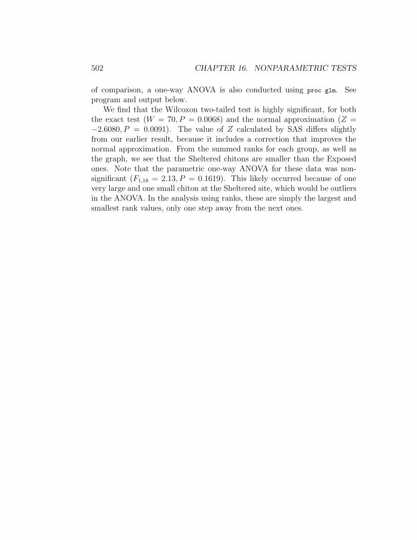
of comparison, a one-way ANOVA is also conducted using proc glm. Seeprogram and output below.

We find that the Wilcoxon two-tailed test is highly significant, for boththe exact test (W = 70, P = 0.0068) and the normal approximation (Z =−2.6080, P = 0.0091). The value of Z calculated by SAS differs slightlyfrom our earlier result, because it includes a correction that improves thenormal approximation. From the summed ranks for each group, as well asthe graph, we see that the Sheltered chitons are smaller than the Exposedones. Note that the parametric one-way ANOVA for these data was non-significant (F1,18 = 2.13, P = 0.1619). This likely occurred because of onevery large and one small chiton at the Sheltered site, which would be outliersin the ANOVA. In the analysis using ranks, these are simply the largest andsmallest rank values, only one step away from the next ones.


SAS Program

* WKWtest_chitons_Venados.sas;

options pageno=1 linesize=80;

goptions reset=all;

title ’Wilcoxon and Kruskal-Wallis tests for chiton length’;

data chitons;

input site :$10. length;

datalines;

Sheltered 44.39

Sheltered 22.30

Sheltered 21.31

Sheltered 23.80

Sheltered 26.23

etc.

;

run;

* Print data set;

proc print data=chitons;

run;

* Plot means, standard error, and observations;

proc gplot data=chitons;

plot length*site / vaxis=axis1 haxis=axis1;

symbol1 i=std1mjt v=star height=2 width=3;

axis1 label=(height=2) value=(height=2) width=3 major=(width=2) minor=none;

run;

* Kruskal-Wallis/Wilcoxon tests;

proc npar1way wilcoxon data=chitons;

class site;

var length;

exact wilcoxon;

run;

* One-way ANOVA for comparison;

proc glm data=chitons;

class site;

model length = site;

output out=resids p=pred r=resid;

run;

quit;


SAS Output

Wilcoxon and Kruskal-Wallis tests for chiton length 1

13:00 Wednesday, November 18, 2015

Obs site length

1 Sheltered 44.39

2 Sheltered 22.30

3 Sheltered 21.31

4 Sheltered 23.80

5 Sheltered 26.23

etc.



The NPAR1WAY Procedure

Wilcoxon Scores (Rank Sums) for Variable length

Classified by Variable site

Sum of Expected Std Dev Mean

site N Scores Under H0 Under H0 Score

Sheltered 10 70.0 105.0 13.228757 7.0

Exposed 10 140.0 105.0 13.228757 14.0

Wilcoxon Two-Sample Test

Statistic (S) 70.0000

Normal Approximation

Z -2.6080

One-Sided Pr < Z 0.0046

Two-Sided Pr > |Z| 0.0091

t Approximation

One-Sided Pr < Z 0.0086

Two-Sided Pr > |Z| 0.0173

Exact Test

One-Sided Pr <= S 0.0034


Two-Sided Pr >= |S - Mean| 0.0068

Z includes a continuity correction of 0.5.

Kruskal-Wallis Test

Chi-Square 7.0000

DF 1

Pr > Chi-Square 0.0082



The GLM Procedure

Class Level Information

Class Levels Values

site 2 Exposed Sheltered

Number of Observations Read 20

Number of Observations Used 20



The GLM Procedure

Dependent Variable: length

Sum of

Source DF Squares Mean Square F Value Pr > F

Model 1 66.4301250 66.4301250 2.13 0.1619

Error 18 562.0077700 31.2226539

Corrected Total 19 628.4378950


R-Square Coeff Var Root MSE length Mean

0.105707 20.37791 5.587723 27.42050

Source DF Type I SS Mean Square F Value Pr > F

site 1 66.43012500 66.43012500 2.13 0.1619

Source DF Type III SS Mean Square F Value Pr > F

site 1 66.43012500 66.43012500 2.13 0.1619

Figure 16.3: Means ± standard errors and individual data points for theExample 1 data.

16.2. KRUSKAL-WALLIS TEST 507

16.2 Kruskal-Wallis test

The Kruskal-Wallis test is an extension of rank methods to one-way designswith three or more groups. The null and alternative hypotheses are similar tothe Wilcoxon test, with the cumulative distributions for the different groupsthe same under H0, and differing by shift parameters under H1. The Kruskal-Wallis test is sensitive to these shifts as well as differences among the meansof the groups.

The Kruskal-Wallis test statistic H is calculated using the ranks of theobservations across all groups. Suppose we have a different groups, and forsimplicity assume the same sample size n for each group. The Kruskal-Wallistest statistic is

H =12n

an(an+ 1)

a∑i=1

(∑nj=1Rij

n− an+ 1

2

)2

(16.6)

(Conover 1999; Hollander et al. 2014). Note that the left term in parenthesesis the mean rank for each group, while the right one is the mean rank acrossall the groups. This implies that H will become large when the mean rankdiffers among groups, similar to the way differences in the group means affectthe F statistic for one-way ANOVA. In fact, the Kruskal-Wallis statistic canbe derived from the F test by substituting ranks for the observations (Bickel& Doksum 1977). A more complex form of H is used when sample sizes areunequal, or when there are ties in the data. Under H0, H has approximatelya χ2 distribution with a− 1 degrees of freedom.

Sample calculations

We will illustrate the Kruskal-Wallis test using both the Example 1 and 2data sets. For Example 1, we have two groups with ten observations each, soa = 2 and n = 10. The summed ranks for the two groups are 70 (Sheltered)


and 140 (Exposed). It follows that

H =12 · 10

2 · 10(2 · 10 + 1)

[(70

10− 2 · 10 + 1

2

)2

+

(140

10− 2 · 10 + 1

2

)2]

=120

420

[(7− 10.5)2 + (14− 10.5)2

]= 0.2857 [12.25 + 12.25]

= 7.00.

The degrees of freedom are a − 1 = 2 − 1 = 1. From Table C, we find thatP < 0.01, and so the Exposed and Sheltered chitons are significantly differentin length (H = 7.00, df = 1, P < 0.01).

The Example 2 data involves chitons collected from three different islands(a = 3), with ten chitons sampled per island (n = 10). The summed ranks forthe three islands are 157, 142, and 166. From this information, we calculatethat

H =12 · 10

3 · 10(3 · 10 + 1)

·

[(157

10− 3 · 10 + 1

2

)2

+

(142

10− 3 · 10 + 1

2

)2

+

(166

10− 3 · 10 + 1

2

)2]

=120

930

[(15.7− 15.5)2 + (14.2− 15.5)2 + (16.6− 15.5)2

]= 0.129 [0.04 + 1.69 + 1.21]

= 0.38.

The degrees of freedom are a − 1 = 3 − 1 = 2. From Table C, we findthat P < 0.9. There was no significant difference in length among the threeislands (H = 0.38, df = 2, P < 0.9).

16.2.1 Kruskal-Wallis test for Example 1 - SAS demo

The Kruskal-Wallis test is automatically calculated when the wilcoxon optionfor proc npar1way is used (see previous SAS output). We see there is a highlysignificant difference in length betwee the Sheltered and Exposed sites (H =7.00, df = 1, P = 0.0082).


16.2.2 Kruskal-Wallis test for Example 2 - SAS demo

The Kruskal-Wallis test for the Example 2 data is shown below. There wasno significant difference in length among the three islands (H = 0.38, df =2, P = 0.8272). Note that an exact version of this test is also provided(P = 0.8386).

SAS Program

* KWtest_chitons_3islands.sas;


goptions reset=all;

title ’Kruskal-Wallis test for chiton length’;

data chitons;

input island $ length;

datalines;

Lobos 23.86

Lobos 20.20

Lobos 29.32

Lobos 23.56

Lobos 24.32

etc.

;

run;

* Print data set;


run;


proc gplot data=chitons;

plot length*island / vaxis=axis1 haxis=axis1;



run;

* Kruskal-Wallis/Wilcoxon tests;

proc npar1way wilcoxon data=chitons;

class island;

var length;

exact wilcoxon;

run;

quit;


SAS Output

Kruskal-Wallis test for chiton length 1

10:24 Wednesday, January 7, 2015

length

Obs island length Rank

1 Lobos 23.86 16

2 Lobos 20.20 6

3 Lobos 29.32 27

4 Lobos 23.56 13

5 Lobos 24.32 17

etc.

Kruskal-Wallis test for chiton length 2



Wilcoxon Scores (Rank Sums) for Variable length

Classified by Variable island

Sum of Expected Std Dev Mean

island N Scores Under H0 Under H0 Score

Lobos 10 157.0 155.0 22.730303 15.70

Pajaros 10 142.0 155.0 22.730303 14.20

Venados 10 166.0 155.0 22.730303 16.60

Kruskal-Wallis Test

Chi-Square 0.3794

DF 2

Asymptotic Pr > Chi-Square 0.8272

Exact Pr >= Chi-Square 0.8386


16.3 Kolmogorov-Smirnov test

The Kolmogorov-Smirnov test is a nonparametric procedure used to comparethe distributions of two samples. Let F1(y) be the cumulative distributionfunction for the first group, while F2(y) is the second. The null hypothesisfor the Kolmogorov-Smirnov test is H0 : F2(y) = F1(y), which means thatthe two groups have the same distribution. The alternative hypothesis isH1 : F2(y) 6= F1(y) for some y, implying there is some difference in thedistributions, which could involve their location, general shape, variance,and so forth. This is a broader alternative hypothesis than the rank tests weexamined earlier, where the distributions had the same shape but differed bylocation.

The Kolmogorov-Smirnov test statistic is calculated using the empiricaldistribution functions of the two samples. These are the empirical counter-parts of the distribution functions defined for distributions like the normal(see Chapter 6). For a sample with ni observations, the empirical distributionfunction is defined as

Gi(y) =Number of Yij values ≤ y

ni. (16.7)

Gi(y) increases in a step-like fashion as y increases, with a jump occurringat every value of Yij (Conover 1999; Hollander et al. 2014). Fig. 16.5 showsthese functions for the two samples in Example 1. The Kolmogorov-Smirnovtest uses the maximum vertical distance between the two functions as thetest statistic. The distance is defined using the formula

D = maxy|G1(y)−G2(y)| (16.8)

(Conover 1999; Hollander et al. 2014). D is the largest distance betweenG1(y) and G2(y) over all values of y, with the absolute value making it apositive quantity. We would then reject H0 for sufficiently large values ofD. The P value for the test can calculated exactly for small sample sizes,and there is also a large sample approximation for the test. We will letSAS handle the details. This test can also be used when there ties in theobservations, in which case it is conservative, meaning it is less likely to rejectH0 (Hollander et al. 2014).

16.3. KOLMOGOROV-SMIRNOV TEST 513

Figure 16.5: Empirical distribution functions for the Example 1 data. Alsoshown is the maximum value of D for the two samples.

16.3.1 Kolmogorov-Smirnov test for Example 1 - SASdemo

The SAS procedure npar1way can also be used for the Kolmogorov-Smirnovtest (SAS Institute Inc. 2014a). It is invoked by adding the edf option inthe proc npar1way statement (see program below). An exact version of testcan also be generated using the line exact ks. The program also includesproc gchart code to generate histograms of the two groups (SAS InstituteInc. 2014b). This seems more appropriate for the Kolmogorov-Smirnov testthan plotting the means, because this test can detect differences in bothshape and location. Examining the SAS output, we see that D = 0.7 (seealso Fig. 16.5). The P value for the exact version of the test is significant(P = 0.0123), implying there is some difference in the distributions of thetwo samples. The graph generated by proc gchart illustrates these differences(Fig. 16.6). See program and output below.


SAS Program

* KStest_chitons_Venados.sas;


goptions reset=all;

title ’Kolmogorov-Smirnov test for chiton length’;

data chitons;

input site :$10. length;

datalines;

Sheltered 44.39

Sheltered 22.30

Sheltered 21.31

Sheltered 23.80

Sheltered 26.23

etc.

;

run;

* Print data set;


run;

* Histograms for the two groups;

proc gchart data=chitons;

vbar length / group=site axis=axis1 gaxis=axis1 maxis=axis2;

axis1 label=(height=2) value=(height=2) width=3 minor=none;

axis2 label=(height=1.5) value=(height=1.5) width=1.5;

run;

* Kolmogorov-Smirnov test;

proc npar1way edf data=chitons;

class site;

var length;

exact ks;

run;

quit;

16.3. KOLMOGOROV-SMIRNOV TEST 515

SAS Output

Kolmogorov-Smirnov test for chiton length 1


Obs site length

1 Sheltered 44.39

2 Sheltered 22.30

3 Sheltered 21.31

4 Sheltered 23.80

5 Sheltered 26.23

etc.

Kolmogorov-Smirnov test for chiton length 2



Kolmogorov-Smirnov Test for Variable length

Classified by Variable site

EDF at Deviation from Mean

site N Maximum at Maximum

Sheltered 10 0.900 1.106797

Exposed 10 0.200 -1.106797

Total 20 0.550

Maximum Deviation Occurred at Observation 7

Value of length at Maximum = 28.10

KS 0.3500 KSa 1.5652

Kolmogorov-Smirnov Two-Sample Test

D = max |F1 - F2| 0.7000

Asymptotic Pr > D 0.0149

Exact Pr >= D 0.0123

D+ = max (F1 - F2) 0.7000

Asymptotic Pr > D+ 0.0074

Exact Pr >= D+ 0.0062


D- = max (F2 - F1) 0.1000

Asymptotic Pr > D- 0.9048

Exact Pr >= D- 0.9091

Figure 16.6: Histograms showing the distribution of lengths for the Example1 data.

16.4 Randomization tests

Randomization tests are another common kind of nonparametric test used forone-way designs, as well as more complex ones (Hinkelmann & Kempthorne1994; Manly 1997). The null hypothesis for these tests is different from othertests we have considered, which involved statements about probability distri-butions and their parameters. For randomization tests, the null hypothesisis that all possible permutations (rearrangements) of the data among groupsare equally likely, given no treatment or group effects, with the observed databeing one such arrangement (Hinkelmann & Kempthorne 1994; Manly 1997).These tests commonly employ a parametric test statistic to examine the nullhypothesis, one that is sensitive to potential differences among groups. Forone-way designs, the Fs statistic from one-way ANOVA (Chapter 11) is often

16.4. RANDOMIZATION TESTS 517

used to detect differences in the group means. To conduct a randomizationtest using this statistic, we first calculate the value of Fs(obs) for the observeddata. Similar to one-way ANOVA, we then need to determine if Fs(obs) issufficiently large to consider rejecting H0. This is accomplished by permutingor rearranging the observations many times across groups, and calculatingthe value of Fs for each permutation. The justification for this procedurefollows directly from the definition of H0. The P value for the test is definedas the proportion of the Fs values greater than or equal to Fs(obs), includingFs(obs) as one of the values.

For small data sets it may be possible to carry out all possible permu-tations, but for larger data sets this may be impractical. Instead, the ob-servations are randomly rearranged across groups a large number of times,in effect drawing a random sample from all possible permutations. The col-lection of Fs values obtained by this process is called the randomizationdistribution. How many of these randomizations are needed to generate anaccurate P value for the test? Some guidance is provided by Manly (1997),who suggests that 1000 randomizations should be sufficient for P ≈ 0.05,and 5000 for P ≈ 0.01.

An interesting feature of randomization tests is that the randomizationdistribution of Fs under H0 can be approximated by the parametric F dis-tribution (Hinkelmann & Kempthorne 1974) under some conditions. Thisprovides another justification for the use of F tests when the normality as-sumption of these tests is violated.

We will use data on nematode intensities for male vs. female bob-cats (Lynx rufus) to illustrate randomization tests. The sampled bobcatswere recent roadkill collected from the Southern Illinois region (FranciscoA. Jimenez-Ruiz and Eliot A. Zieman, unpublished data). The guts wereexamined for nematodes as well as other parasites, and the total numbercounted (Table 16.3). These data have many zeroes as well as large values,as is common for parasite intensity data. The data are clearly non-normaland so a nonparametric test seems warranted.


Table 16.3: Example 3 - Number of nematode parasites found in the gut ofmale and female bobcats collected from Southern Illinois .

Sex Nematodes Sex Nematodes Sex Nematodes Sex NematodesF 0 F 0 M 6 M 8F 8 F 5 M 10 M 0F 0 F 0 M 1 M 60F 0 F 0 M 0 M 25F 0 F 0 M 5 M 1F 0 F 11 M 59 M 0F 0 F 0 M 2 M 74F 1 F 5 M 3 M 3F 2 F 11 M 0 M 1F 1 F 0 M 44 M 15F 1 F 24 M 1 M 0F 6 F 13 M 1 M 7F 1 F 2 M 0 M 0F 6 M 2 M 0F 2 M 17F 1 M 5F 13 M 3F 0 M 26F 0 M 20F 7 M 3


16.4.1 Randomization test for Example 3 - SAS demo

We will analyze the bobcat data using both one-way ANOVA and the anal-ogous randomization test, comparing the parasite intensities for male vs.female cats. The SAS program below first generates a graph showing themean intensities for both sexes, then conducts a standard one-way ANOVA.We see that the mean intensity for male bobcats is higher than females (Fig.16.7), and the ANOVA shows this difference is significant (F1,65 = 5.50, P =0.0221).

The program then uses two SAS macro programs to conduct the random-ization test (Cassell 2002). SAS macros are chunks of code that are used tocarry out custom calculations, ones not available in standard SAS procedures(SAS Institute Inc. 2014c). They are inserted into a main program throughthe use of %include statements, which point to the file locations of the macros.Note that the percent sign (%) in tells SAS that a particular line containsmacro code. The first macro, %rand_gen.sas, is used to generate the desirednumber of random permutations of the data. Once the macro is included inthe program, it can be called using the following arguments. The input dataset is specified using the indata=parasites statement, while the output dataset specified by outdata=outrand contains all the randomizations. The state-ment numreps=5000 sets the number of randomizations, with the dependentvariable specified by depvar=nematodes.

The next step in the randomization test is to conduct a one-way ANOVAfor each one of the randomizations, as well as the original data set. Thisis accomplished using proc glm with a by replicate statement. The variablereplicate is generated by the rand_gen macro to number the different ran-domizations. In addition, a data file containing the statistical output of theANOVA is specified using the statement outstat=outstat1. The ANOVA forthe original data corresponds to a replicate = 0 in this output file. Thenoprint option is used to suppress the printing of each ANOVA.

The last step in the randomization test uses the second macro, %rand_anl.sas,to determine the P value for the test. The data file containing the statis-tical output from proc glm is specified using a randdata=outstat1 argument.The where=_source_=’sex’ and _type_=’SS3’ argument tells the macro whichpart of the statistical output to use, in particular the test associated withthe sex effect and Type III sum of squares. The testprob=prob statementtells the macro to use the P value for this F test in calculating the P valuefor the randomization test. The macro uses the P rather than Fs value to


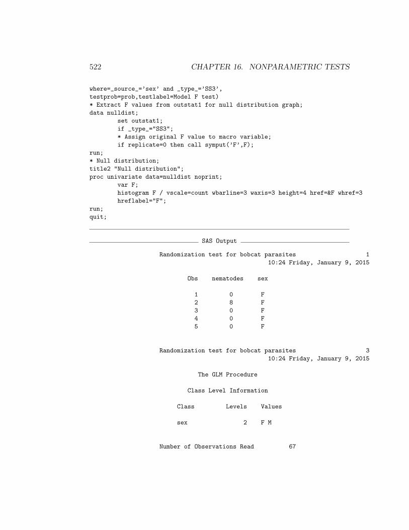
provide some additional flexibility for other kinds of tests (Cassell 2002).As the Fs and P value for the ANOVA are related, it yields the same re-sult. The P value for the randomization test is provided in the SAS log.The testlabel=Model F test argument provides some labeling for this output.Examining the SAS log, we find that the randomization test is significant(P = 0.0172). The P value for this test is smaller than the one found usingone-way ANOVA, and makes no assumptions about the distribution of thedata.

The remaining portion of the program generates a graph of the random-ization distribution of Fs, and displays the value of this statistic for theoriginal distribution. We see that the original value of Fs lies far above mostof the randomizations. This illustrates the pattern for a significant random-ization test. For a non-significant test, we would see an Fs value that is morecentral within the randomization distribution.


SAS Program

* Randtest_bobcat_parasites.sas;


goptions reset=all;

title ’Randomization test for bobcat parasites’;

data parasites;

input nematodes sex $;

datalines;

0 F

8 F

0 F

0 F

0 F

etc.

;

run;

* Print data set;

proc print data=parasites;

run;


proc gplot data=parasites;

plot nematodes*sex / vaxis=axis1 haxis=axis1;



run;

* One-way ANOVA;

proc glm data=parasites;

class sex;

model nematodes = sex;

run;

* Include two macros for randomization test;

%include "C:\Users\John\Documents\My Documents\Nonparametric\rand_gen.sas";

%include "C:\Users\John\Documents\My Documents\Nonparametric\rand_anl.sas";

* One-way ANOVA as a randomization test;

%rand_gen(indata=parasites,outdata=outrand,

depvar=nematodes,numreps=5000)

proc glm data=outrand noprint outstat=outstat1;

by replicate;

class sex;

model nematodes = sex;

run;

%rand_anl(randdata=outstat1,


where=_source_=’sex’ and _type_=’SS3’,

testprob=prob,testlabel=Model F test)

* Extract F values from outstat1 for null distribution graph;

data nulldist;

set outstat1;

if _type_="SS3";

* Assign original F value to macro variable;

if replicate=0 then call symput(’F’,F);

run;

* Null distribution;

title2 "Null distribution";

proc univariate data=nulldist noprint;

var F;

histogram F / vscale=count wbarline=3 waxis=3 height=4 href=&F whref=3

hreflabel="F";

run;

quit;

SAS Output

Randomization test for bobcat parasites 1

10:24 Friday, January 9, 2015

Obs nematodes sex

1 0 F

2 8 F

3 0 F

4 0 F

5 0 F



The GLM Procedure

Class Level Information

Class Levels Values

sex 2 F M

Number of Observations Read 67


Number of Observations Used 67



The GLM Procedure

Dependent Variable: nematodes

Sum of

Source DF Squares Mean Square F Value Pr > F

Model 1 1122.49709 1122.49709 5.50 0.0221

Error 65 13274.57754 204.22427

Corrected Total 66 14397.07463

R-Square Coeff Var Root MSE nematodes Mean

0.077967 183.4248 14.29071 7.791045

Source DF Type I SS Mean Square F Value Pr > F

sex 1 1122.497087 1122.497087 5.50 0.0221

Source DF Type III SS Mean Square F Value Pr > F

sex 1 1122.497087 1122.497087 5.50 0.0221

SAS Log

Randomization test for Model F test where _source_=’sex’ and _type_=’SS3’

has significance level of 0.0172



Figure 16.8: Distribution of F under the null hypothesis, obtained throughrandomization.

16.5. LIMITATIONS OF NONPARAMETRIC TESTS 525

16.5 Limitations of nonparametric tests

While nonparametric tests can be useful for non-normal data, they do havesome drawbacks. One is that the number of designs that have nonparametrictests are fairly limited. We have seen tests nonparametric tests analogousto one-way ANOVA and two-sample t tests. There is also a rank test forrandomized block designs called Friedman’s test, as well as procedures formultiple comparisons (Hollander et al. 2014). Unfortunately, for more com-plex designs there are few available procedures.

Although nonparametric tests are not based on a particular distribution,they do make some assumptions. Consider the null and alternative hypothe-ses for the Wilcoxon test. The two groups are assumed to have the samecumulative distribution function, differing only by a shift parameter ∆. Thisimplies the two groups have the same variance under both hypotheses, simi-lar to parametric ones. When the variances are unequal as well as the samplesizes, both parametric and nonparametric tests may not be valid (Stewart-Oaten 1995). In particular, they may not have the correct Type I errorrate.

Table 16.4 illustrates how unequal variances and sample sizes can affectthe Type I error rate. It summarizes a simulation study comparing thevalidity of several different methods of comparing samples from two groups,including parametric and nonparametric methods. The first six columnsgive the theoretical mean, variance, and the sample sizes for the two groups.The simulated data were normally distributed with these parameters. Eachdata set was then analyzed using a two-sample t test, a Welch t test thatimplements a correction for unequal variances, the Wilcoxon test, and arandomization test. Any significant differences detected by these tests areType I errors, because the two groups have the same mean. A total of5000 simulated data sets were generated and analyzed. The proportion ofsimulated data sets showing significant results is an estimate of the TypeI error rate (α) for each test. If the test is conducted using α = 0.05, forexample, we would expect this proportion of the simulations to be significant.

Regardless of differences in the variance between the two groups, whenthe sample sizes are equal all methods yield a Type I error rate near thenominal α = 0.05 level. When sample sizes are unequal, the t test, Wilcoxontest, and the randomization test all yield Type I error rates higher or lowerthan α = 0.05. Note that the pattern depends on which group (high or lowvariance) has the smaller sample size. Thus, the validity of these procedures


depends on equal variances, especially when sample sizes are unequal acrossgroups. This assumption needs to be carefully examined within applyingboth parametric and nonparametric tests.

The only valid test in this scenario was the Welch t test, which employs acorrection for unequal variances. The correction alters the degrees of freedomfor the test, based on the sample sizes and variances of the two groups (Stuartet al. 1999). It is conducted automatically by proc ttest in SAS, withthe output labeled Satterthwaite (see Chapter 11). There is also a similarprocedure for one-way designs called Welch ANOVA. It can conducted underproc glm using the welch option for the means statement.

Table 16.4: Effect of unequal variances and sample sizes on the estimatedType I error rate for common parametric and nonparametric tests, usingα = 0.05 for all tests. See text for further details.

µ1 σ21 n1 µ2 σ2

2 n2 t Welch Wilcoxon Randomization10 1 10 10 1 10 0.0474 0.0454 0.0422 0.048410 1 10 10 2 10 0.0516 0.0504 0.0514 0.052410 1 5 10 2 15 0.0208 0.0510 0.0236 0.021410 1 15 10 2 5 0.0956 0.0578 0.0662 0.095410 1 10 10 4 10 0.0510 0.0452 0.0464 0.051010 1 5 10 4 15 0.0104 0.0494 0.0170 0.010810 1 15 10 4 5 0.1588 0.0574 0.0836 0.1598

16.6. PROBLEMS 527

16.6 Problems

1. Using the Example 3 data, conduct a Wilcoxon test comparing parasiteintensity in male vs. female bobcats. How do the results compare tothe randomization test for these data in the text?

2. Data were also collected on the number of cestode parasites found in thebobcats from Example 3 (see below). Cestodes are another commontype of gut parasite. Conduct a randomization test comparing thecestode intensity for male vs. female bobcats.

Sex Cestodes Sex Cestodes Sex Cestodes Sex CestodesF 1 F 0 M 9 M 3F 7 F 7 M 31 M 2F 9 F 6 M 5 M 2F 0 F 33 M 0 M 0F 1 F 2 M 10 M 3F 1 F 1 M 6 M 7F 8 F 18 M 0 M 2F 0 F 6 M 0 M 5F 0 F 1 M 6 M 1F 32 F 14 M 9 M 1F 11 F 12 M 6 M 4F 4 F 6 M 18 M 0F 3 F 0 M 4 M 3F 13 M 9 M 1F 2 M 6F 2 M 5F 12 M 17F 4 M 4F 1 M 8F 3 M 11


16.7 References

Cassell, D. L. (2002) A randomization-test wrapper for SAS PROCs. SUGI27: Paper 251-27.

Conover, W. J. (1999) Practical Nonparametric Statistics. John Wiley &Sons, Inc., New York, NY.

Flores-Campana, L. M., Arzola-Gonzalez, J. F., & Leon-Herrera, R. (2012)Body size structure, biometric relationships and density of Chiton albo-lineatus (Mollusca: Polyplacophora) on the intertidal rocky zone of threeislands of Mazatlan Bay, SE of the Gulf of California. Revista de BiologiaMarina y Oceanographıa 47: 203-211.

Glass, G. V., Peckham, P. D., & Sanders, J. R. (1972) Consequences offailure to meet assumptions underlying fixed effects analysis of varianceand covariance. Review of Educational Research 42: 237-288.

Hinkelmann, K., & Kempthorne, O. (1994) Design and Analysis of Exper-iments, Volume I: Introduction to Experimental Design. John Wiley &Sons, Inc., New York, NY.

Hollander, M., Wolfe, D. A., & Chicken, E. (2014) Nonparametric StatisticalMethods, Third Edition. John Wiley & Sons, Inc., Hoboken, NJ.

SAS Institute Inc. (2014a) SAS/STAT 13.2 Users Guide. SAS Institute Inc.,Cary, NC.

SAS Institute Inc. (2014b) SAS/GRAPH 9.4: Reference, Third Edition.SAS Institute Inc., Cary, NC.

SAS Institute Inc. (2014c) SAS 9.4 Macro Language: Reference, FourthEdition. SAS Institute Inc., Cary, NC.

Stuart, A., Ord, J. K., & Arnold, S. (1999) Kendall’s Advanced Theory ofStatistics, Volume 2A, Classical Inference and the Linear Model. OxfordUniversity Press Inc., New York, NY.

Manly, B. F. J. (1997) Randomization, Bootstrap, and Monte Carlo Methodsin Biology. Chapman & Hall, New York, NY.