chapter 12: boundary-value problems in rectangular...
TRANSCRIPT
Separation of Variables and Classical PDE’sWave Equation
Laplace’s EquationSummary
Chapter 12: Boundary-Value Problems inRectangular Coordinates
王奕翔
Department of Electrical EngineeringNational Taiwan University
December 21, 2013
1 / 50 王奕翔 DE Lecture 14
Separation of Variables and Classical PDE’sWave Equation
Laplace’s EquationSummary
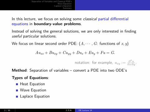
In this lecture, we focus on solving some classical partial differentialequations in boundary-value problems.Instead of solving the general solutions, we are only interested in findinguseful particular solutions.We focus on linear second order PDE: (A, · · · ,G: functions of x, y)
Auxx + Buxy + Cuyy + Dux + Euy + Fu = G.
notation: for example, uxy := ∂2u∂x ∂y .
Method: Separation of variables – convert a PDE into two ODE’sTypes of Equations:
Heat EquationWave EquationLaplace Equation
2 / 50 王奕翔 DE Lecture 14
Separation of Variables and Classical PDE’sWave Equation
Laplace’s EquationSummary
Classification of Linear Second Order PDE
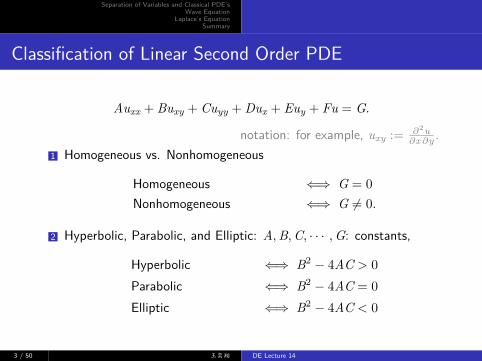
Auxx + Buxy + Cuyy + Dux + Euy + Fu = G.
notation: for example, uxy := ∂2u∂x ∂y .
1 Homogeneous vs. Nonhomogeneous
Homogeneous ⇐⇒ G = 0
Nonhomogeneous ⇐⇒ G ̸= 0.
2 Hyperbolic, Parabolic, and Elliptic: A,B,C, · · · ,G: constants,
Hyperbolic ⇐⇒ B2 − 4AC > 0
Parabolic ⇐⇒ B2 − 4AC = 0
Elliptic ⇐⇒ B2 − 4AC < 0
3 / 50 王奕翔 DE Lecture 14
Separation of Variables and Classical PDE’sWave Equation
Laplace’s EquationSummary
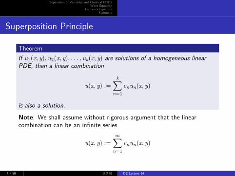
Superposition Principle
TheoremIf u1(x, y), u2(x, y), . . . , uk(x, y) are solutions of a homogeneous linearPDE, then a linear combination
u(x, y) :=k∑
n=1
cnun(x, y)
is also a solution.
Note: We shall assume without rigorous argument that the linearcombination can be an infinite series
u(x, y) :=∞∑
n=1
cnun(x, y)
4 / 50 王奕翔 DE Lecture 14
Separation of Variables and Classical PDE’sWave Equation
Laplace’s EquationSummary
1 Separation of Variables and Classical PDE’s
2 Wave Equation
3 Laplace’s Equation
4 Summary
5 / 50 王奕翔 DE Lecture 14
Separation of Variables and Classical PDE’sWave Equation
Laplace’s EquationSummary
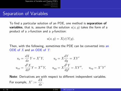
Separation of Variables
To find a particular solution of an PDE, one method is separation ofvariables, that is, assume that the solution u(x, y) takes the form of aproduct of a x-function and a y-function:
u(x, y) = X(x)Y(y).
Then, with the following, sometimes the PDE can be converted into anODE of X and an ODE of Y:
ux =dXdx Y = X ′Y, uy = XdY
dy = XY ′
uxx =d2Xdx2 Y = X ′′Y, uyy = Xd2Y
dy2 = XY ′′, uxy = X ′Y ′
Note: Derivatives are with respect to different independent variables.For example, X ′ :=
dXdx .
6 / 50 王奕翔 DE Lecture 14
Separation of Variables and Classical PDE’sWave Equation
Laplace’s EquationSummary
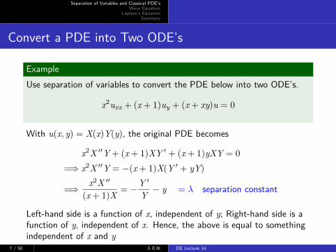
Convert a PDE into Two ODE’s
ExampleUse separation of variables to convert the PDE below into two ODE’s.
x2uxx + (x + 1)uy + (x + xy)u = 0
With u(x, y) = X(x)Y(y), the original PDE becomes
x2X ′′Y + (x + 1)XY ′ + (x + 1)yXY = 0
=⇒ x2X ′′Y = −(x + 1)X(Y ′ + yY)
=⇒ x2X ′′
(x + 1)X = −Y ′
Y − y = λ separation constant
Left-hand side is a function of x, independent of y; Right-hand side is afunction of y, independent of x. Hence, the above is equal to somethingindependent of x and y
7 / 50 王奕翔 DE Lecture 14
Separation of Variables and Classical PDE’sWave Equation
Laplace’s EquationSummary
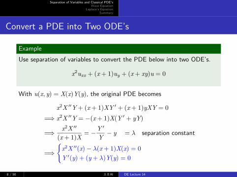
Convert a PDE into Two ODE’s
ExampleUse separation of variables to convert the PDE below into two ODE’s.
x2uxx + (x + 1)uy + (x + xy)u = 0
With u(x, y) = X(x)Y(y), the original PDE becomes
x2X ′′Y + (x + 1)XY ′ + (x + 1)yXY = 0
=⇒ x2X ′′Y = −(x + 1)X(Y ′ + yY)
=⇒ x2X ′′
(x + 1)X = −Y ′
Y − y = λ separation constant
=⇒{
x2X ′′(x)− λ(x + 1)X(x) = 0
Y ′(y) + (y + λ)Y(y) = 0
8 / 50 王奕翔 DE Lecture 14
Separation of Variables and Classical PDE’sWave Equation
Laplace’s EquationSummary
Some Remarks
1 The method of separation of variables can only solve for some linearsecond order PDE’s, not all of them.
2 For the PDE’s considered in this lecture, the method works.
3 The method may work for both homogeneous (G = 0) andnonhomogeneous (G ̸= 0) PDE’s
Auxx + Buxy + Cuyy + Dux + Euy + Fu = G.
9 / 50 王奕翔 DE Lecture 14
Separation of Variables and Classical PDE’sWave Equation
Laplace’s EquationSummary
Three Classical PDE’s
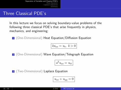
In this lecture we focus on solving boundary-value problems of thefollowing three classical PDE’s that arise frequently in physics,mechanics, and engineering:
1 (One-Dimensional) Heat Equation/Diffusion Equation
kuxx = ut, k > 0
2 (One-Dimensional) Wave Equation/Telegraph Equation
a2uxx = utt
3 (Two-Dimensional) Laplace Equation
uxx + uyy = 0
10 / 50 王奕翔 DE Lecture 14
Separation of Variables and Classical PDE’sWave Equation
Laplace’s EquationSummary
Heat Transfer within a Thin Rod: Heat Equation
variables. If you compare (1)–(3) with the linear form in Theorem 12.1.1 (with t play-ing the part of the symbol y), observe that the heat equation (1) is parabolic, the waveequation (2) is hyperbolic, and Laplace’s equation is elliptic. This observation will beimportant in Chapter 15.
Heat Equation Equation (1) occurs in the theory of heat flow—that is, heattransferred by conduction in a rod or in a thin wire. The function u(x, t) representstemperature at a point x along the rod at some time t. Problems in mechanical vibra-tions often lead to the wave equation (2). For purposes of discussion, a solutionu(x, t) of (2) will represent the displacement of an idealized string. Finally, a solutionu(x, y) of Laplace’s equation (3) can be interpreted as the steady-state (that is, time-independent) temperature distribution throughout a thin, two-dimensional plate.
Even though we have to make many simplifying assumptions, it is worthwhileto see how equations such as (1) and (2) arise.
Suppose a thin circular rod of length L has a cross-sectional area A and coin-cides with the x-axis on the interval [0, L]. See Figure 12.2.1. Let us suppose thefollowing:
• The flow of heat within the rod takes place only in the x-direction.• The lateral, or curved, surface of the rod is insulated; that is, no heat
escapes from this surface.• No heat is being generated within the rod.• The rod is homogeneous; that is, its mass per unit volume r is a constant.• The specific heat g and thermal conductivity K of the material of the rod are
constants.
To derive the partial differential equation satisfied by the temperature u(x, t), weneed two empirical laws of heat conduction:
(i) The quantity of heat Q in an element of mass m is
, (4)
where u is the temperature of the element.
(ii) The rate of heat flow Qt through the cross-section indicated inFigure 12.2.1 is proportional to the area A of the cross section andthe partial derivative with respect to x of the temperature:
. (5)
Since heat flows in the direction of decreasing temperature, the minus sign in (5) isused to ensure that Qt is positive for ux ! 0 (heat flow to the right) and negative forux " 0 (heat flow to the left). If the circular slice of the rod shown in Figure 12.2.1between x and x # $x is very thin, then u(x, t) can be taken as the approximate tem-perature at each point in the interval. Now the mass of the slice is m % r(A $x), andso it follows from (4) that the quantity of heat in it is
. (6)
Furthermore, when heat flows in the positive x-direction, we see from (5) that heatbuilds up in the slice at the net rate
. (7)
By differentiating (6) with respect to t, we see that this net rate is also given by
. (8)
Equating (7) and (8) gives
. (9)K&'
ux(x # $x, t) ( ux(x, t)
$x% ut
Qt % &'A $x ut
(KAux(x, t) ( [(KAux(x # $x, t)] % KA [ux(x # $x, t) ( ux(x, t)]
Q % &'A $x u
Qt % (KAux
Q % &mu
12.2 CLASSICAL PDEs AND BOUNDARY-VALUE PROBLEMS ! 461
x0 x x + !x L
Cross section of area A
FIGURE 12.2.1 One-dimensionalflow of heat
92467_12_ch12_p455-492.qxd 2/16/12 11:41 AM Page 461
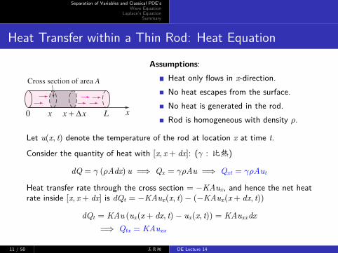
Assumptions:Heat only flows in x-direction.No heat escapes from the surface.No heat is generated in the rod.Rod is homogeneous with density ρ.
Let u(x, t) denote the temperature of the rod at location x at time t.
Consider the quantity of heat with [x, x + dx]: (γ : 比熱)
dQ = γ (ρAdx) u =⇒ Qx = γρAu =⇒ Qxt = γρAut
Heat transfer rate through the cross section = −KAux, and hence the net heatrate inside [x, x + dx] is dQt = −KAux(x, t)− (−KAux(x + dx, t))
dQt = KAu (ux(x + dx, t)− ux(x, t)) = KAuxxdx=⇒ Qtx = KAuxx
11 / 50 王奕翔 DE Lecture 14
Separation of Variables and Classical PDE’sWave Equation
Laplace’s EquationSummary
Heat Transfer within a Thin Rod: Heat Equation
variables. If you compare (1)–(3) with the linear form in Theorem 12.1.1 (with t play-ing the part of the symbol y), observe that the heat equation (1) is parabolic, the waveequation (2) is hyperbolic, and Laplace’s equation is elliptic. This observation will beimportant in Chapter 15.
Heat Equation Equation (1) occurs in the theory of heat flow—that is, heattransferred by conduction in a rod or in a thin wire. The function u(x, t) representstemperature at a point x along the rod at some time t. Problems in mechanical vibra-tions often lead to the wave equation (2). For purposes of discussion, a solutionu(x, t) of (2) will represent the displacement of an idealized string. Finally, a solutionu(x, y) of Laplace’s equation (3) can be interpreted as the steady-state (that is, time-independent) temperature distribution throughout a thin, two-dimensional plate.
Even though we have to make many simplifying assumptions, it is worthwhileto see how equations such as (1) and (2) arise.
Suppose a thin circular rod of length L has a cross-sectional area A and coin-cides with the x-axis on the interval [0, L]. See Figure 12.2.1. Let us suppose thefollowing:
• The flow of heat within the rod takes place only in the x-direction.• The lateral, or curved, surface of the rod is insulated; that is, no heat
escapes from this surface.• No heat is being generated within the rod.• The rod is homogeneous; that is, its mass per unit volume r is a constant.• The specific heat g and thermal conductivity K of the material of the rod are
constants.
To derive the partial differential equation satisfied by the temperature u(x, t), weneed two empirical laws of heat conduction:
(i) The quantity of heat Q in an element of mass m is
, (4)
where u is the temperature of the element.
(ii) The rate of heat flow Qt through the cross-section indicated inFigure 12.2.1 is proportional to the area A of the cross section andthe partial derivative with respect to x of the temperature:
. (5)
Since heat flows in the direction of decreasing temperature, the minus sign in (5) isused to ensure that Qt is positive for ux ! 0 (heat flow to the right) and negative forux " 0 (heat flow to the left). If the circular slice of the rod shown in Figure 12.2.1between x and x # $x is very thin, then u(x, t) can be taken as the approximate tem-perature at each point in the interval. Now the mass of the slice is m % r(A $x), andso it follows from (4) that the quantity of heat in it is
. (6)
Furthermore, when heat flows in the positive x-direction, we see from (5) that heatbuilds up in the slice at the net rate
. (7)
By differentiating (6) with respect to t, we see that this net rate is also given by
. (8)
Equating (7) and (8) gives
. (9)K&'
ux(x # $x, t) ( ux(x, t)
$x% ut
Qt % &'A $x ut
(KAux(x, t) ( [(KAux(x # $x, t)] % KA [ux(x # $x, t) ( ux(x, t)]
Q % &'A $x u
Qt % (KAux
Q % &mu
12.2 CLASSICAL PDEs AND BOUNDARY-VALUE PROBLEMS ! 461
x0 x x + !x L
Cross section of area A
FIGURE 12.2.1 One-dimensionalflow of heat
92467_12_ch12_p455-492.qxd 2/16/12 11:41 AM Page 461
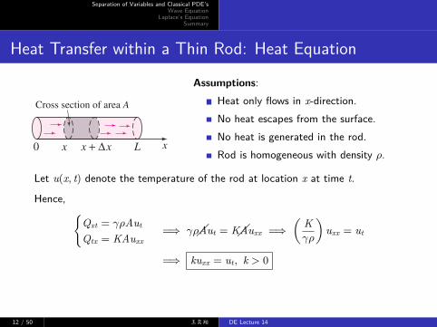
Assumptions:Heat only flows in x-direction.No heat escapes from the surface.No heat is generated in the rod.Rod is homogeneous with density ρ.
Let u(x, t) denote the temperature of the rod at location x at time t.
Hence, {Qxt = γρAut
Qtx = KAuxx=⇒ γρ�Aut = K�Auxx =⇒
(Kγρ
)uxx = ut
=⇒ kuxx = ut, k > 0
12 / 50 王奕翔 DE Lecture 14
Separation of Variables and Classical PDE’sWave Equation
Laplace’s EquationSummary
Heat Equation: Initial and Boundary Conditions
variables. If you compare (1)–(3) with the linear form in Theorem 12.1.1 (with t play-ing the part of the symbol y), observe that the heat equation (1) is parabolic, the waveequation (2) is hyperbolic, and Laplace’s equation is elliptic. This observation will beimportant in Chapter 15.
Heat Equation Equation (1) occurs in the theory of heat flow—that is, heattransferred by conduction in a rod or in a thin wire. The function u(x, t) representstemperature at a point x along the rod at some time t. Problems in mechanical vibra-tions often lead to the wave equation (2). For purposes of discussion, a solutionu(x, t) of (2) will represent the displacement of an idealized string. Finally, a solutionu(x, y) of Laplace’s equation (3) can be interpreted as the steady-state (that is, time-independent) temperature distribution throughout a thin, two-dimensional plate.
Even though we have to make many simplifying assumptions, it is worthwhileto see how equations such as (1) and (2) arise.
Suppose a thin circular rod of length L has a cross-sectional area A and coin-cides with the x-axis on the interval [0, L]. See Figure 12.2.1. Let us suppose thefollowing:
• The flow of heat within the rod takes place only in the x-direction.• The lateral, or curved, surface of the rod is insulated; that is, no heat
escapes from this surface.• No heat is being generated within the rod.• The rod is homogeneous; that is, its mass per unit volume r is a constant.• The specific heat g and thermal conductivity K of the material of the rod are
constants.
To derive the partial differential equation satisfied by the temperature u(x, t), weneed two empirical laws of heat conduction:
(i) The quantity of heat Q in an element of mass m is
, (4)
where u is the temperature of the element.
(ii) The rate of heat flow Qt through the cross-section indicated inFigure 12.2.1 is proportional to the area A of the cross section andthe partial derivative with respect to x of the temperature:
. (5)
Since heat flows in the direction of decreasing temperature, the minus sign in (5) isused to ensure that Qt is positive for ux ! 0 (heat flow to the right) and negative forux " 0 (heat flow to the left). If the circular slice of the rod shown in Figure 12.2.1between x and x # $x is very thin, then u(x, t) can be taken as the approximate tem-perature at each point in the interval. Now the mass of the slice is m % r(A $x), andso it follows from (4) that the quantity of heat in it is
. (6)
Furthermore, when heat flows in the positive x-direction, we see from (5) that heatbuilds up in the slice at the net rate
. (7)
By differentiating (6) with respect to t, we see that this net rate is also given by
. (8)
Equating (7) and (8) gives
. (9)K&'
ux(x # $x, t) ( ux(x, t)
$x% ut
Qt % &'A $x ut
(KAux(x, t) ( [(KAux(x # $x, t)] % KA [ux(x # $x, t) ( ux(x, t)]
Q % &'A $x u
Qt % (KAux
Q % &mu
12.2 CLASSICAL PDEs AND BOUNDARY-VALUE PROBLEMS ! 461
x0 x x + !x L
Cross section of area A
FIGURE 12.2.1 One-dimensionalflow of heat
92467_12_ch12_p455-492.qxd 2/16/12 11:41 AM Page 461
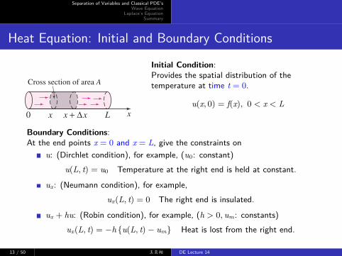
Initial Condition:Provides the spatial distribution of thetemperature at time t = 0.
u(x, 0) = f(x), 0 < x < L
Boundary Conditions:At the end points x = 0 and x = L, give the constraints on
u: (Dirchlet condition), for example, (u0: constant)u(L, t) = u0 Temperature at the right end is held at constant.
ux: (Neumann condition), for example,ux(L, t) = 0 The right end is insulated.
ux + hu: (Robin condition), for example, (h > 0, um: constants)ux(L, t) = −h {u(L, t)− um} Heat is lost from the right end.
13 / 50 王奕翔 DE Lecture 14
Separation of Variables and Classical PDE’sWave Equation
Laplace’s EquationSummary
Heat Equation: Boundary-Value Problems
variables. If you compare (1)–(3) with the linear form in Theorem 12.1.1 (with t play-ing the part of the symbol y), observe that the heat equation (1) is parabolic, the waveequation (2) is hyperbolic, and Laplace’s equation is elliptic. This observation will beimportant in Chapter 15.
Heat Equation Equation (1) occurs in the theory of heat flow—that is, heattransferred by conduction in a rod or in a thin wire. The function u(x, t) representstemperature at a point x along the rod at some time t. Problems in mechanical vibra-tions often lead to the wave equation (2). For purposes of discussion, a solutionu(x, t) of (2) will represent the displacement of an idealized string. Finally, a solutionu(x, y) of Laplace’s equation (3) can be interpreted as the steady-state (that is, time-independent) temperature distribution throughout a thin, two-dimensional plate.
Even though we have to make many simplifying assumptions, it is worthwhileto see how equations such as (1) and (2) arise.
Suppose a thin circular rod of length L has a cross-sectional area A and coin-cides with the x-axis on the interval [0, L]. See Figure 12.2.1. Let us suppose thefollowing:
• The flow of heat within the rod takes place only in the x-direction.• The lateral, or curved, surface of the rod is insulated; that is, no heat
escapes from this surface.• No heat is being generated within the rod.• The rod is homogeneous; that is, its mass per unit volume r is a constant.• The specific heat g and thermal conductivity K of the material of the rod are
constants.
To derive the partial differential equation satisfied by the temperature u(x, t), weneed two empirical laws of heat conduction:
(i) The quantity of heat Q in an element of mass m is
, (4)
where u is the temperature of the element.
(ii) The rate of heat flow Qt through the cross-section indicated inFigure 12.2.1 is proportional to the area A of the cross section andthe partial derivative with respect to x of the temperature:
. (5)
Since heat flows in the direction of decreasing temperature, the minus sign in (5) isused to ensure that Qt is positive for ux ! 0 (heat flow to the right) and negative forux " 0 (heat flow to the left). If the circular slice of the rod shown in Figure 12.2.1between x and x # $x is very thin, then u(x, t) can be taken as the approximate tem-perature at each point in the interval. Now the mass of the slice is m % r(A $x), andso it follows from (4) that the quantity of heat in it is
. (6)
Furthermore, when heat flows in the positive x-direction, we see from (5) that heatbuilds up in the slice at the net rate
. (7)
By differentiating (6) with respect to t, we see that this net rate is also given by
. (8)
Equating (7) and (8) gives
. (9)K&'
ux(x # $x, t) ( ux(x, t)
$x% ut
Qt % &'A $x ut
(KAux(x, t) ( [(KAux(x # $x, t)] % KA [ux(x # $x, t) ( ux(x, t)]
Q % &'A $x u
Qt % (KAux
Q % &mu
12.2 CLASSICAL PDEs AND BOUNDARY-VALUE PROBLEMS ! 461
x0 x x + !x L
Cross section of area A
FIGURE 12.2.1 One-dimensionalflow of heat
92467_12_ch12_p455-492.qxd 2/16/12 11:41 AM Page 461
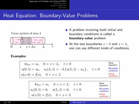
A problem involving both initial andboundary conditions is called aboundary-value problemAt the two boundaries x − 0 and x = L,one can use different kinds of conditions.
Examples:
kuxx = ut, 0 < x < L, t > 0 Heatequation
u(0, t) = u0, ux(L, t) = −h {u(L, t)− um} , t > 0 Boundarycondition
u(x, 0) = f(x), 0 < x < L Initialcondition
kuxx = ut, 0 < x < L, t > 0 Heatequation
ux(0, t) = 0, u(L, t) = 0, t > 0 Boundarycondition
u(x, 0) = f(x), 0 < x < L Initialcondition
14 / 50 王奕翔 DE Lecture 14
Separation of Variables and Classical PDE’sWave Equation
Laplace’s EquationSummary
Dynamics of a String Fixed at Two Ends: Wave Equation462 ! CHAPTER 12 BOUNDARY-VALUE PROBLEMS IN RECTANGULAR COORDINATES
Finally, by taking the limit of (9) as we obtain (1) in the form*
(K!gr)uxx ! ut. It is customary to let k ! K!gr and call this positive constant thethermal diffusivity.
Wave Equation Consider a string of length L, such as a guitar string,stretched taut between two points on the x-axis—say, x ! 0 and x ! L. When thestring starts to vibrate, assume that the motion takes place in the xu-plane in sucha manner that each point on the string moves in a direction perpendicular to the x-axis(transverse vibrations). As is shown in Figure 12.2.2(a), let u(x, t) denote the verticaldisplacement of any point on the string measured from the x-axis for t " 0. We fur-ther assume the following:
• The string is perfectly flexible.• The string is homogeneous; that is, its mass per unit length r is a
constant.• The displacements u are small in comparison to the length of the string.• The slope of the curve is small at all points.• The tension T acts tangent to the string, and its magnitude T is the same at
all points.• The tension is large compared with the force of gravity.• No other external forces act on the string.
Now in Figure 12.2.2(b) the tensions T1 and T2 are tangent to the ends of thecurve on the interval [x, x # $x]. For small u1 and u2 the net vertical force acting onthe corresponding element $s of the string is then
where T ! "T1 " ! "T2 ". Now r $s # r $x is the mass of the string on [x, x # $x],so Newton’s second law gives
or
If the limit is taken as the last equation becomes uxx ! (r!T)utt. This ofcourse is (2) with a2 ! T!r.
Laplace’s Equation Although we shall not present its derivation, Laplace’sequation in two and three dimensions occurs in time-independent problems involv-ing potentials such as electrostatic, gravitational, and velocity in fluid mechanics.Moreover, a solution of Laplace’s equation can also be interpreted as a steady-statetemperature distribution. As illustrated in Figure 12.2.3, a solution u(x, y) of (3)could represent the temperature that varies from point to point—but not with time—of a rectangular plate. Laplace’s equation in two dimensions and in three dimensionsis abbreviated as %2u ! 0, where
are called the two-dimensional Laplacian and the three-dimensional Laplacian,respectively, of a function u.
%2u !&2u&x2 #
&2u&y2 and %2u !
&2u&x2 #
&2u&y2 #
&2u&z2
$x : 0,
ux(x # $x, t) ' ux(x, t)
$x!
(
T ut t.
T [ux(x # $x, t) ' ux(x, t)] ! ( $x ut t
! T [ux(x # $x, t) ' ux(x, t)],† T sin )2 ' T sin )1 # T tan )2 ' T tan )1
$x : 0,
u
!su(x, t)
0 x x + !x L x
x
u
!s
x + !xx
"1
" 2
T1
T2
(a) Segment of string
(b) Enlargement of segment
FIGURE 12.2.2 Flexible stringanchored at x ! 0 and x ! L
100
60
0
120
80
?F–20
180
160
140
20
40
200
220
(x, y)
y
ThermometerTemperature as afunction of positionon the hot plate
W
O
xH
FIGURE 12.2.3 Steady-statetemperatures in a rectangular plate
*The definition of the second partial derivative is †tan u2 ! ux(x # $x, t) and tan u1 ! ux(x, t) are equivalent expressions for slope.
uxx ! lim$x : 0
ux(x # $x, t) ' ux(x, t)$x
.
92467_12_ch12_p455-492.qxd 2/16/12 11:41 AM Page 462
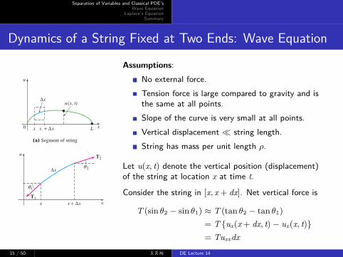
Assumptions:No external force.Tension force is large compared to gravity and isthe same at all points.Slope of the curve is very small at all points.Vertical displacement ≪ string length.String has mass per unit length ρ.
Let u(x, t) denote the vertical position (displacement)of the string at location x at time t.
Consider the string in [x, x + dx]. Net vertical force is
T (sin θ2 − sin θ1) ≈ T (tan θ2 − tan θ1)
= T {ux(x + dx, t)− ux(x, t)}= Tuxxdx
15 / 50 王奕翔 DE Lecture 14
Separation of Variables and Classical PDE’sWave Equation
Laplace’s EquationSummary
Dynamics of a String Fixed at Two Ends: Wave Equation462 ! CHAPTER 12 BOUNDARY-VALUE PROBLEMS IN RECTANGULAR COORDINATES
Finally, by taking the limit of (9) as we obtain (1) in the form*
(K!gr)uxx ! ut. It is customary to let k ! K!gr and call this positive constant thethermal diffusivity.
Wave Equation Consider a string of length L, such as a guitar string,stretched taut between two points on the x-axis—say, x ! 0 and x ! L. When thestring starts to vibrate, assume that the motion takes place in the xu-plane in sucha manner that each point on the string moves in a direction perpendicular to the x-axis(transverse vibrations). As is shown in Figure 12.2.2(a), let u(x, t) denote the verticaldisplacement of any point on the string measured from the x-axis for t " 0. We fur-ther assume the following:
• The string is perfectly flexible.• The string is homogeneous; that is, its mass per unit length r is a
constant.• The displacements u are small in comparison to the length of the string.• The slope of the curve is small at all points.• The tension T acts tangent to the string, and its magnitude T is the same at
all points.• The tension is large compared with the force of gravity.• No other external forces act on the string.
Now in Figure 12.2.2(b) the tensions T1 and T2 are tangent to the ends of thecurve on the interval [x, x # $x]. For small u1 and u2 the net vertical force acting onthe corresponding element $s of the string is then
where T ! "T1 " ! "T2 ". Now r $s # r $x is the mass of the string on [x, x # $x],so Newton’s second law gives
or
If the limit is taken as the last equation becomes uxx ! (r!T)utt. This ofcourse is (2) with a2 ! T!r.
Laplace’s Equation Although we shall not present its derivation, Laplace’sequation in two and three dimensions occurs in time-independent problems involv-ing potentials such as electrostatic, gravitational, and velocity in fluid mechanics.Moreover, a solution of Laplace’s equation can also be interpreted as a steady-statetemperature distribution. As illustrated in Figure 12.2.3, a solution u(x, y) of (3)could represent the temperature that varies from point to point—but not with time—of a rectangular plate. Laplace’s equation in two dimensions and in three dimensionsis abbreviated as %2u ! 0, where
are called the two-dimensional Laplacian and the three-dimensional Laplacian,respectively, of a function u.
%2u !&2u&x2 #
&2u&y2 and %2u !
&2u&x2 #
&2u&y2 #
&2u&z2
$x : 0,
ux(x # $x, t) ' ux(x, t)
$x!
(
T ut t.
T [ux(x # $x, t) ' ux(x, t)] ! ( $x ut t
! T [ux(x # $x, t) ' ux(x, t)],† T sin )2 ' T sin )1 # T tan )2 ' T tan )1
$x : 0,
u
!su(x, t)
0 x x + !x L x
x
u
!s
x + !xx
"1
" 2
T1
T2
(a) Segment of string
(b) Enlargement of segment
FIGURE 12.2.2 Flexible stringanchored at x ! 0 and x ! L
100
60
0
120
80
?F–20
180
160
140
20
40
200
220
(x, y)
y
ThermometerTemperature as afunction of positionon the hot plate
W
O
xH
FIGURE 12.2.3 Steady-statetemperatures in a rectangular plate
*The definition of the second partial derivative is †tan u2 ! ux(x # $x, t) and tan u1 ! ux(x, t) are equivalent expressions for slope.
uxx ! lim$x : 0
ux(x # $x, t) ' ux(x, t)$x
.
92467_12_ch12_p455-492.qxd 2/16/12 11:41 AM Page 462
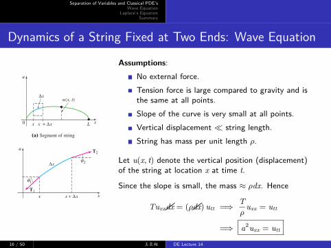
Assumptions:No external force.Tension force is large compared to gravity and isthe same at all points.Slope of the curve is very small at all points.Vertical displacement ≪ string length.String has mass per unit length ρ.
Let u(x, t) denote the vertical position (displacement)of the string at location x at time t.
Since the slope is small, the mass ≈ ρdx. Hence
Tuxx��dx = (ρ��dx) utt =⇒ Tρ
uxx = utt
=⇒ a2uxx = utt
16 / 50 王奕翔 DE Lecture 14
Separation of Variables and Classical PDE’sWave Equation
Laplace’s EquationSummary
Wave Equation: Initial and Boundary Conditions462 ! CHAPTER 12 BOUNDARY-VALUE PROBLEMS IN RECTANGULAR COORDINATES
Finally, by taking the limit of (9) as we obtain (1) in the form*
(K!gr)uxx ! ut. It is customary to let k ! K!gr and call this positive constant thethermal diffusivity.
Wave Equation Consider a string of length L, such as a guitar string,stretched taut between two points on the x-axis—say, x ! 0 and x ! L. When thestring starts to vibrate, assume that the motion takes place in the xu-plane in sucha manner that each point on the string moves in a direction perpendicular to the x-axis(transverse vibrations). As is shown in Figure 12.2.2(a), let u(x, t) denote the verticaldisplacement of any point on the string measured from the x-axis for t " 0. We fur-ther assume the following:
• The string is perfectly flexible.• The string is homogeneous; that is, its mass per unit length r is a
constant.• The displacements u are small in comparison to the length of the string.• The slope of the curve is small at all points.• The tension T acts tangent to the string, and its magnitude T is the same at
all points.• The tension is large compared with the force of gravity.• No other external forces act on the string.
Now in Figure 12.2.2(b) the tensions T1 and T2 are tangent to the ends of thecurve on the interval [x, x # $x]. For small u1 and u2 the net vertical force acting onthe corresponding element $s of the string is then
where T ! "T1 " ! "T2 ". Now r $s # r $x is the mass of the string on [x, x # $x],so Newton’s second law gives
or
If the limit is taken as the last equation becomes uxx ! (r!T)utt. This ofcourse is (2) with a2 ! T!r.
Laplace’s Equation Although we shall not present its derivation, Laplace’sequation in two and three dimensions occurs in time-independent problems involv-ing potentials such as electrostatic, gravitational, and velocity in fluid mechanics.Moreover, a solution of Laplace’s equation can also be interpreted as a steady-statetemperature distribution. As illustrated in Figure 12.2.3, a solution u(x, y) of (3)could represent the temperature that varies from point to point—but not with time—of a rectangular plate. Laplace’s equation in two dimensions and in three dimensionsis abbreviated as %2u ! 0, where
are called the two-dimensional Laplacian and the three-dimensional Laplacian,respectively, of a function u.
%2u !&2u&x2 #
&2u&y2 and %2u !
&2u&x2 #
&2u&y2 #
&2u&z2
$x : 0,
ux(x # $x, t) ' ux(x, t)
$x!
(
T ut t.
T [ux(x # $x, t) ' ux(x, t)] ! ( $x ut t
! T [ux(x # $x, t) ' ux(x, t)],† T sin )2 ' T sin )1 # T tan )2 ' T tan )1
$x : 0,
u
!su(x, t)
0 x x + !x L x
x
u
!s
x + !xx
"1
" 2
T1
T2
(a) Segment of string
(b) Enlargement of segment
FIGURE 12.2.2 Flexible stringanchored at x ! 0 and x ! L
100
60
0
120
80
?F–20
180
160
140
20
40
200
220
(x, y)
y
ThermometerTemperature as afunction of positionon the hot plate
W
O
xH
FIGURE 12.2.3 Steady-statetemperatures in a rectangular plate
*The definition of the second partial derivative is †tan u2 ! ux(x # $x, t) and tan u1 ! ux(x, t) are equivalent expressions for slope.
uxx ! lim$x : 0
ux(x # $x, t) ' ux(x, t)$x
.
92467_12_ch12_p455-492.qxd 2/16/12 11:41 AM Page 462
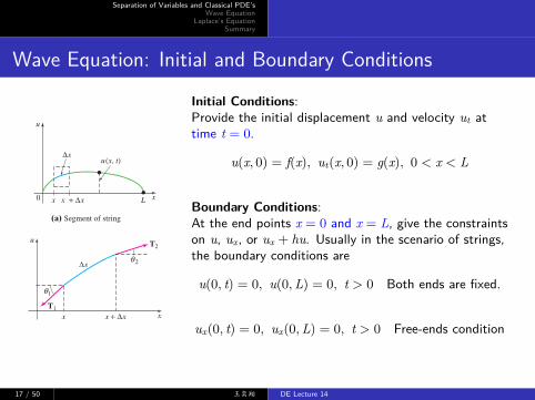
Initial Conditions:Provide the initial displacement u and velocity ut attime t = 0.
u(x, 0) = f(x), ut(x, 0) = g(x), 0 < x < L
Boundary Conditions:At the end points x = 0 and x = L, give the constraintson u, ux, or ux + hu. Usually in the scenario of strings,the boundary conditions are
u(0, t) = 0, u(0,L) = 0, t > 0 Both ends are fixed.
ux(0, t) = 0, ux(0,L) = 0, t > 0 Free-ends condition
17 / 50 王奕翔 DE Lecture 14
Separation of Variables and Classical PDE’sWave Equation
Laplace’s EquationSummary
Wave Equation: Boundary-Value Problems462 ! CHAPTER 12 BOUNDARY-VALUE PROBLEMS IN RECTANGULAR COORDINATES
Finally, by taking the limit of (9) as we obtain (1) in the form*
(K!gr)uxx ! ut. It is customary to let k ! K!gr and call this positive constant thethermal diffusivity.
Wave Equation Consider a string of length L, such as a guitar string,stretched taut between two points on the x-axis—say, x ! 0 and x ! L. When thestring starts to vibrate, assume that the motion takes place in the xu-plane in sucha manner that each point on the string moves in a direction perpendicular to the x-axis(transverse vibrations). As is shown in Figure 12.2.2(a), let u(x, t) denote the verticaldisplacement of any point on the string measured from the x-axis for t " 0. We fur-ther assume the following:
• The string is perfectly flexible.• The string is homogeneous; that is, its mass per unit length r is a
constant.• The displacements u are small in comparison to the length of the string.• The slope of the curve is small at all points.• The tension T acts tangent to the string, and its magnitude T is the same at
all points.• The tension is large compared with the force of gravity.• No other external forces act on the string.
Now in Figure 12.2.2(b) the tensions T1 and T2 are tangent to the ends of thecurve on the interval [x, x # $x]. For small u1 and u2 the net vertical force acting onthe corresponding element $s of the string is then
where T ! "T1 " ! "T2 ". Now r $s # r $x is the mass of the string on [x, x # $x],so Newton’s second law gives
or
If the limit is taken as the last equation becomes uxx ! (r!T)utt. This ofcourse is (2) with a2 ! T!r.
Laplace’s Equation Although we shall not present its derivation, Laplace’sequation in two and three dimensions occurs in time-independent problems involv-ing potentials such as electrostatic, gravitational, and velocity in fluid mechanics.Moreover, a solution of Laplace’s equation can also be interpreted as a steady-statetemperature distribution. As illustrated in Figure 12.2.3, a solution u(x, y) of (3)could represent the temperature that varies from point to point—but not with time—of a rectangular plate. Laplace’s equation in two dimensions and in three dimensionsis abbreviated as %2u ! 0, where
are called the two-dimensional Laplacian and the three-dimensional Laplacian,respectively, of a function u.
%2u !&2u&x2 #
&2u&y2 and %2u !
&2u&x2 #
&2u&y2 #
&2u&z2
$x : 0,
ux(x # $x, t) ' ux(x, t)
$x!
(
T ut t.
T [ux(x # $x, t) ' ux(x, t)] ! ( $x ut t
! T [ux(x # $x, t) ' ux(x, t)],† T sin )2 ' T sin )1 # T tan )2 ' T tan )1
$x : 0,
u
!su(x, t)
0 x x + !x L x
x
u
!s
x + !xx
"1
" 2
T1
T2
(a) Segment of string
(b) Enlargement of segment
FIGURE 12.2.2 Flexible stringanchored at x ! 0 and x ! L
100
60
0
120
80
?F–20
180
160
140
20
40
200
220
(x, y)
y
ThermometerTemperature as afunction of positionon the hot plate
W
O
xH
FIGURE 12.2.3 Steady-statetemperatures in a rectangular plate
*The definition of the second partial derivative is †tan u2 ! ux(x # $x, t) and tan u1 ! ux(x, t) are equivalent expressions for slope.
uxx ! lim$x : 0
ux(x # $x, t) ' ux(x, t)$x
.
92467_12_ch12_p455-492.qxd 2/16/12 11:41 AM Page 462
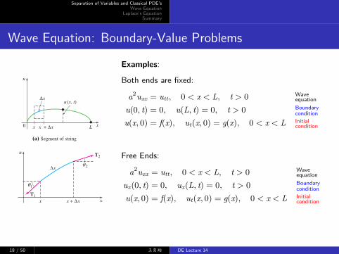
Examples:
Both ends are fixed:
a2uxx = utt, 0 < x < L, t > 0 Waveequation
u(0, t) = 0, u(L, t) = 0, t > 0 Boundarycondition
u(x, 0) = f(x), ut(x, 0) = g(x), 0 < x < L Initialcondition
Free Ends:
a2uxx = utt, 0 < x < L, t > 0 Waveequation
ux(0, t) = 0, ux(L, t) = 0, t > 0 Boundarycondition
u(x, 0) = f(x), ut(x, 0) = g(x), 0 < x < L Initialcondition
18 / 50 王奕翔 DE Lecture 14
Separation of Variables and Classical PDE’sWave Equation
Laplace’s EquationSummary
Laplace’s Equation
462 ! CHAPTER 12 BOUNDARY-VALUE PROBLEMS IN RECTANGULAR COORDINATES
Finally, by taking the limit of (9) as we obtain (1) in the form*
(K!gr)uxx ! ut. It is customary to let k ! K!gr and call this positive constant thethermal diffusivity.
Wave Equation Consider a string of length L, such as a guitar string,stretched taut between two points on the x-axis—say, x ! 0 and x ! L. When thestring starts to vibrate, assume that the motion takes place in the xu-plane in sucha manner that each point on the string moves in a direction perpendicular to the x-axis(transverse vibrations). As is shown in Figure 12.2.2(a), let u(x, t) denote the verticaldisplacement of any point on the string measured from the x-axis for t " 0. We fur-ther assume the following:
• The string is perfectly flexible.• The string is homogeneous; that is, its mass per unit length r is a
constant.• The displacements u are small in comparison to the length of the string.• The slope of the curve is small at all points.• The tension T acts tangent to the string, and its magnitude T is the same at
all points.• The tension is large compared with the force of gravity.• No other external forces act on the string.
Now in Figure 12.2.2(b) the tensions T1 and T2 are tangent to the ends of thecurve on the interval [x, x # $x]. For small u1 and u2 the net vertical force acting onthe corresponding element $s of the string is then
where T ! "T1 " ! "T2 ". Now r $s # r $x is the mass of the string on [x, x # $x],so Newton’s second law gives
or
If the limit is taken as the last equation becomes uxx ! (r!T)utt. This ofcourse is (2) with a2 ! T!r.
Laplace’s Equation Although we shall not present its derivation, Laplace’sequation in two and three dimensions occurs in time-independent problems involv-ing potentials such as electrostatic, gravitational, and velocity in fluid mechanics.Moreover, a solution of Laplace’s equation can also be interpreted as a steady-statetemperature distribution. As illustrated in Figure 12.2.3, a solution u(x, y) of (3)could represent the temperature that varies from point to point—but not with time—of a rectangular plate. Laplace’s equation in two dimensions and in three dimensionsis abbreviated as %2u ! 0, where
are called the two-dimensional Laplacian and the three-dimensional Laplacian,respectively, of a function u.
%2u !&2u&x2 #
&2u&y2 and %2u !
&2u&x2 #
&2u&y2 #
&2u&z2
$x : 0,
ux(x # $x, t) ' ux(x, t)
$x!
(
T ut t.
T [ux(x # $x, t) ' ux(x, t)] ! ( $x ut t
! T [ux(x # $x, t) ' ux(x, t)],† T sin )2 ' T sin )1 # T tan )2 ' T tan )1
$x : 0,
u
!su(x, t)
0 x x + !x L x
x
u
!s
x + !xx
"1
" 2
T1
T2
(a) Segment of string
(b) Enlargement of segment
FIGURE 12.2.2 Flexible stringanchored at x ! 0 and x ! L
100
60
0
120
80
?F–20
180
160
140
20
40
200
220
(x, y)
y
ThermometerTemperature as afunction of positionon the hot plate
W
O
xH
FIGURE 12.2.3 Steady-statetemperatures in a rectangular plate
*The definition of the second partial derivative is †tan u2 ! ux(x # $x, t) and tan u1 ! ux(x, t) are equivalent expressions for slope.
uxx ! lim$x : 0
ux(x # $x, t) ' ux(x, t)$x
.
92467_12_ch12_p455-492.qxd 2/16/12 11:41 AM Page 462
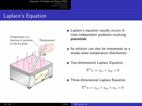
Laplace’s equation usually occurs intime-independent problems involvingpotentials.
Its solution can also be interpreted as asteady-state temperature distribution.
Two-dimensional Laplace Equation
∇2u := uxx + uyy = 0
Three-dimensional Laplace Equation
∇2u := uxx + uyy + uzz = 0
19 / 50 王奕翔 DE Lecture 14
Separation of Variables and Classical PDE’sWave Equation
Laplace’s EquationSummary
Laplace’s Equation: Boundary Conditions
462 ! CHAPTER 12 BOUNDARY-VALUE PROBLEMS IN RECTANGULAR COORDINATES
Finally, by taking the limit of (9) as we obtain (1) in the form*
(K!gr)uxx ! ut. It is customary to let k ! K!gr and call this positive constant thethermal diffusivity.
Wave Equation Consider a string of length L, such as a guitar string,stretched taut between two points on the x-axis—say, x ! 0 and x ! L. When thestring starts to vibrate, assume that the motion takes place in the xu-plane in sucha manner that each point on the string moves in a direction perpendicular to the x-axis(transverse vibrations). As is shown in Figure 12.2.2(a), let u(x, t) denote the verticaldisplacement of any point on the string measured from the x-axis for t " 0. We fur-ther assume the following:
• The string is perfectly flexible.• The string is homogeneous; that is, its mass per unit length r is a
constant.• The displacements u are small in comparison to the length of the string.• The slope of the curve is small at all points.• The tension T acts tangent to the string, and its magnitude T is the same at
all points.• The tension is large compared with the force of gravity.• No other external forces act on the string.
Now in Figure 12.2.2(b) the tensions T1 and T2 are tangent to the ends of thecurve on the interval [x, x # $x]. For small u1 and u2 the net vertical force acting onthe corresponding element $s of the string is then
where T ! "T1 " ! "T2 ". Now r $s # r $x is the mass of the string on [x, x # $x],so Newton’s second law gives
or
If the limit is taken as the last equation becomes uxx ! (r!T)utt. This ofcourse is (2) with a2 ! T!r.
Laplace’s Equation Although we shall not present its derivation, Laplace’sequation in two and three dimensions occurs in time-independent problems involv-ing potentials such as electrostatic, gravitational, and velocity in fluid mechanics.Moreover, a solution of Laplace’s equation can also be interpreted as a steady-statetemperature distribution. As illustrated in Figure 12.2.3, a solution u(x, y) of (3)could represent the temperature that varies from point to point—but not with time—of a rectangular plate. Laplace’s equation in two dimensions and in three dimensionsis abbreviated as %2u ! 0, where
are called the two-dimensional Laplacian and the three-dimensional Laplacian,respectively, of a function u.
%2u !&2u&x2 #
&2u&y2 and %2u !
&2u&x2 #
&2u&y2 #
&2u&z2
$x : 0,
ux(x # $x, t) ' ux(x, t)
$x!
(
T ut t.
T [ux(x # $x, t) ' ux(x, t)] ! ( $x ut t
! T [ux(x # $x, t) ' ux(x, t)],† T sin )2 ' T sin )1 # T tan )2 ' T tan )1
$x : 0,
u
!su(x, t)
0 x x + !x L x
x
u
!s
x + !xx
"1
" 2
T1
T2
(a) Segment of string
(b) Enlargement of segment
FIGURE 12.2.2 Flexible stringanchored at x ! 0 and x ! L
100
60
0
120
80
?F–20
180
160
140
20
40
200
220
(x, y)
y
ThermometerTemperature as afunction of positionon the hot plate
W
O
xH
FIGURE 12.2.3 Steady-statetemperatures in a rectangular plate
*The definition of the second partial derivative is †tan u2 ! ux(x # $x, t) and tan u1 ! ux(x, t) are equivalent expressions for slope.
uxx ! lim$x : 0
ux(x # $x, t) ' ux(x, t)$x
.
92467_12_ch12_p455-492.qxd 2/16/12 11:41 AM Page 462
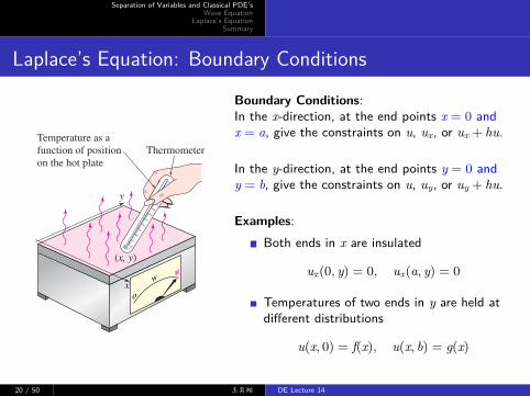
Boundary Conditions:In the x-direction, at the end points x = 0 andx = a, give the constraints on u, ux, or ux + hu.
In the y-direction, at the end points y = 0 andy = b, give the constraints on u, uy, or uy + hu.
Examples:Both ends in x are insulated
ux(0, y) = 0, ux(a, y) = 0
Temperatures of two ends in y are held atdifferent distributions
u(x, 0) = f(x), u(x, b) = g(x)
20 / 50 王奕翔 DE Lecture 14
Separation of Variables and Classical PDE’sWave Equation
Laplace’s EquationSummary
Laplace’s Equation: Boundary-Value Problems
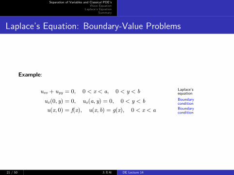
Example:
uxx + uyy = 0, 0 < x < a, 0 < y < b Laplace’sequation
ux(0, y) = 0, ux(a, y) = 0, 0 < y < b Boundarycondition
u(x, 0) = f(x), u(x, b) = g(x), 0 < x < a Boundarycondition
21 / 50 王奕翔 DE Lecture 14
Separation of Variables and Classical PDE’sWave Equation
Laplace’s EquationSummary
Modifications of Heat and Wave Equations
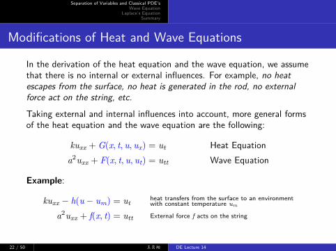
In the derivation of the heat equation and the wave equation, we assumethat there is no internal or external influences. For example, no heatescapes from the surface, no heat is generated in the rod, no externalforce act on the string, etc.Taking external and internal influences into account, more general formsof the heat equation and the wave equation are the following:
kuxx + G(x, t, u, ux) = ut Heat Equationa2uxx + F(x, t, u, ut) = utt Wave Equation
Example:
kuxx − h(u − um) = utheat transfers from the surface to an environmentwith constant temperature um
a2uxx + f(x, t) = utt External force f acts on the string
22 / 50 王奕翔 DE Lecture 14
Separation of Variables and Classical PDE’sWave Equation
Laplace’s EquationSummary
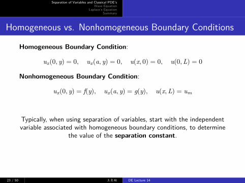
Homogeneous vs. Nonhomogeneous Boundary Conditions
Homogeneous Boundary Condition:
ux(0, y) = 0, ux(a, y) = 0, u(x, 0) = 0, u(0,L) = 0
Nonhomogeneous Boundary Condition:
ux(0, y) = f(y), ux(a, y) = g(y), u(x,L) = um
Typically, when using separation of variables, start with the independentvariable associated with homogeneous boundary conditions, to determine
the value of the separation constant.
23 / 50 王奕翔 DE Lecture 14
Separation of Variables and Classical PDE’sWave Equation
Laplace’s EquationSummary
1 Separation of Variables and Classical PDE’s
2 Wave Equation
3 Laplace’s Equation
4 Summary
24 / 50 王奕翔 DE Lecture 14

Separation of Variables and Classical PDE’sWave Equation
Laplace’s EquationSummary
Wave Equation: a Boundary-Value Problem
Solve u(x, t) : auxx = utt, 0 < x < L, t > 0
subject to : u(0, t) = 0, u(L, t) = 0, t > 0
u(x, 0) = f(x), ut(x, 0) = g(x), 0 < x < L
We focus on solving the above BVP (both ends are fixed).
Step 1: Separation of variables:Assume that the solution u(x, t) = X(x)T(t), X,T ̸= 0. Then,
a2uxx = utt =⇒ a2X ′′T = XT ′′ =⇒ X ′′
X =T ′′
a2T = −λ
=⇒{
X ′′ + λX = 0
T ′′ + a2λT = 0
The 2 homogeneous boundary conditions become X(0) = X(L) = 0.
25 / 50 王奕翔 DE Lecture 14
Separation of Variables and Classical PDE’sWave Equation
Laplace’s EquationSummary
Solve in the x-Dimension and Find λ
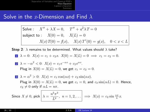
Solve : X ′′ + λX = 0, T ′′ + a2λT = 0
subject to : X(0) = 0, X(L) = 0
X(x)T(0) = f(x), X(x)T ′(0) = g(x), 0 < x < L
Step 2: λ remains to be determined. What values should λ take?1 λ = 0: X(x) = c1 + c2x. X(0) = X(L) = 0 =⇒ c1 = c2 = 0.
2 λ = −α2 < 0: X(x) = c1e−αx + c2eαx.Plug in X(0) = X(L) = 0, we get c1 = c2 = 0.
3 λ = α2 > 0: X(x) = c1 cos(αx) + c2 sin(αx).Plug in X(0) = X(L) = 0, we get c1 = 0, and c2 sin(αL) = 0. Hence,c2 ̸= 0 only if αL = nπ.
Since X ̸= 0, pick λ =n2π2
L2, n = 1, 2, . . . =⇒ X(x) = c2 sin nπ
L x.
26 / 50 王奕翔 DE Lecture 14
Separation of Variables and Classical PDE’sWave Equation
Laplace’s EquationSummary
Solve in t-Dimension and Superposition
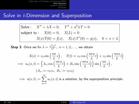
Solve : X ′′ + λX = 0, T ′′ + a2λT = 0
subject to : X(0) = 0, X(L) = 0
X(x)T(0) = f(x), X(x)T ′(0) = g(x), 0 < x < L
Step 3: Once we fix λ = n2π2
L2 , n = 1, 2, . . ., we obtain
X(x) = c2 sin(nπ
L x), T(t) = c3 cos
(nπaL t
)+ c4 sin
(nπaL t
)=⇒ un(x, t) =
{An cos
(nπaL t
)+ Bn sin
(nπaL t
)}sin
(nπL x
),
(An := c2c3, Bn := c2c4)
=⇒ u(x, t) :=∞∑
n=1
un(x, t) is a solution, by the superposition principle.
27 / 50 王奕翔 DE Lecture 14
Separation of Variables and Classical PDE’sWave Equation
Laplace’s EquationSummary
Plug in Initial Condition, Revoke Fourier Series, and Done
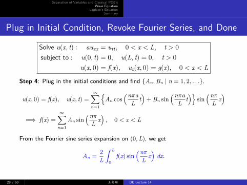
Solve u(x, t) : auxx = utt, 0 < x < L, t > 0
subject to : u(0, t) = 0, u(L, t) = 0, t > 0
u(x, 0) = f(x), ut(x, 0) = g(x), 0 < x < L
Step 4: Plug in the initial conditions and find {An,Bn | n = 1, 2, . . .}.
u(x, 0) = f(x), u(x, t) =∞∑
n=1
{An cos
(nπaL t
)+ Bn sin
(nπaL t
)}sin
(nπL x
)=⇒ f(x) =
∞∑n=1
An sin(nπ
L x), 0 < x < L
From the Fourier sine series expansion on (0,L), we get
An =2
L
∫ L
0
f(x) sin(nπ
L x)
dx.
28 / 50 王奕翔 DE Lecture 14
Separation of Variables and Classical PDE’sWave Equation
Laplace’s EquationSummary
Plug in Initial Condition, Revoke Fourier Series, and Done
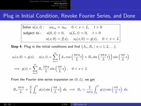
Solve u(x, t) : auxx = utt, 0 < x < L, t > 0
subject to : u(0, t) = 0, u(L, t) = 0, t > 0
u(x, 0) = f(x), ut(x, 0) = g(x), 0 < x < L
Step 4: Plug in the initial conditions and find {An,Bn | n = 1, 2, . . .}.
ut(x, 0) = g(x), u(x, t) =∞∑
n=1
{An cos
(nπaL t
)+ Bn sin
(nπaL t
)}sin
(nπL x
)=⇒ g(x) =
∞∑n=1
BnnπaL sin
(nπL x
), 0 < x < L
From the Fourier sine series expansion on (0,L), we get
BnnπaL =
2
L
∫ L
0
g(x) sin(nπ
L x)
dx. =⇒ Bn =2
nπa
∫ L
0
g(x) sin(nπ
L x)
dx.
29 / 50 王奕翔 DE Lecture 14

Separation of Variables and Classical PDE’sWave Equation
Laplace’s EquationSummary
Final Solution
Solve u(x, t) : auxx = utt, 0 < x < L, t > 0
subject to : u(0, t) = 0, u(L, t) = 0, t > 0
u(x, 0) = f(x), ut(x, 0) = g(x), 0 < x < L
Step 5: The final solution is
u(x, t) =∞∑
n=1
{An cos
(nπaL t
)+ Bn sin
(nπaL t
)}sin
(nπL x
)=
∞∑n=1
Cn sin(nπa
L t + ϕn
)sin
(nπL x
)An =
2
L
∫ L
0
f(x) sin(nπ
L x)
dx, Bn =2
nπa
∫ L
0
g(x) sin(nπ
L x)
dx
Cn =√
A2n + B2n, sinϕn =An
Cn, cosϕn =
Bn
Cn
30 / 50 王奕翔 DE Lecture 14
Separation of Variables and Classical PDE’sWave Equation
Laplace’s EquationSummary
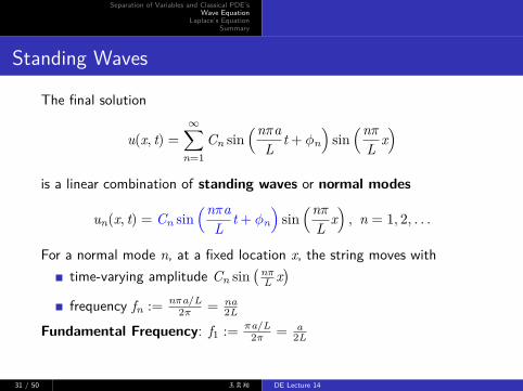
Standing Waves
The final solution
u(x, t) =∞∑
n=1
Cn sin(nπa
L t + ϕn
)sin
(nπL x
)is a linear combination of standing waves or normal modes
un(x, t) = Cn sin(nπa
L t + ϕn
)sin
(nπL x
), n = 1, 2, . . .
For a normal mode n, at a fixed location x, the string moves withtime-varying amplitude Cn sin
(nπL x
)frequency fn := nπa/L
2π = na2L
Fundamental Frequency: f1 := πa/L2π = a
2L
31 / 50 王奕翔 DE Lecture 14
Separation of Variables and Classical PDE’sWave Equation
Laplace’s EquationSummary
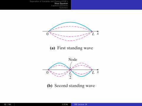
is called the first standing wave, the first normal mode, or the fundamentalmode of vibration. The first three standing waves, or normal modes, are shown inFigure 12.4.2. The dashed graphs represent the standing waves at various values oftime. The points in the interval (0, L), for which sin(np!L)x ! 0, correspond topoints on a standing wave where there is no motion. These points are called nodes.For example, in Figures 12.4.2(b) and 12.4.2(c) we see that the second standingwave has one node at L!2 and the third standing wave has two nodes at L!3 and2L!3. In general, the nth normal mode of vibration has n " 1 nodes.
The frequency
of the first normal mode is called the fundamental frequency or first harmonic andis directly related to the pitch produced by a stringed instrument. It is apparent thatthe greater the tension on the string, the higher the pitch of the sound. Thefrequencies fn of the other normal modes, which are integer multiples of the funda-mental frequency, are called overtones. The second harmonic is the first overtone,and so on.
f1 !a
2L!
12L
BT#
12.4 WAVE EQUATION ! 471
0 L
(a) First standing wave
(b) Second standing wave
(c) Third standing wave
Node
0 LL2
Nodes
0 LL3
2L3
x
x
x
FIGURE 12.4.2 First three standingwaves
FIGURE 12.4.4 Initial displacement in Problem 3
LL/3 2L/3
f (x)
x
1
3. u(0, t) ! 0, u(L, t) ! 0
u(x, 0) given in Figure 12.4.4,$u$t "
t!0! 0
FIGURE 12.4.3 Vibrating elastic bar in Problem 2
x
0 L
u(x, t)
EXERCISES 12.4 Answers to selected odd-numbered problems begin on page ANS-22.
In Problems 1–8 solve the wave equation (1) subject to thegiven conditions.
1.
2.
This problem could describe the longitudinal displace-ment u(x, t) of a vibrating elastic bar. The boundaryconditions at x ! 0 and x ! L are called free-endconditions. See Figure 12.4.3.
u(x, 0) ! x, $u$t "
t!0! 0
$u$x "
x!0! 0, $u
$x "x!L
! 0
u(x, 0) !14
x (L " x), $u$t "
t!0! 0
u(0, t) ! 0, u(L, t) ! 0
4.
5.
6.
7. u(0, t) ! 0, u(L, t) ! 0
8. u(0, t) ! 0, u(1, t) ! 0
u(x, 0) ! 0.01 sin 3px,
9. A string is stretched and secured on the x-axis at x ! 0and x ! p for t % 0. If the transverse vibrations takeplace in a medium that imparts a resistance proportionalto the instantaneous velocity, then the wave equationtakes on the form
$2u$x2 !
$2u$t2 & 2'
$u$t
, 0 ( ' ( 1, t % 0.
$u$t "
t!0! 0
u(x, 0) ! #2hxL
,
2h$1 "xL%,
0 ( x (L2
L2
) x ( L, $u
$t "t!0
! 0
$u$t "
t!0 ! 0u(x, 0) ! 1
6 x(*2 " x2),
u(0, t) ! 0, u(*, t) ! 0
u(x, 0) ! 0, $u$t "
t!0 ! sin x
u(0, t) ! 0, u(*, t) ! 0
u(x, 0) ! 0, $u$t "
t!0! x (L " x)
u(0, t) ! 0, u(L, t) ! 0
aaaaaa.qxd 3/2/12 7:57 AM Page 471
32 / 50 王奕翔 DE Lecture 14
Separation of Variables and Classical PDE’sWave Equation
Laplace’s EquationSummary
1 Separation of Variables and Classical PDE’s
2 Wave Equation
3 Laplace’s Equation
4 Summary
33 / 50 王奕翔 DE Lecture 14
Separation of Variables and Classical PDE’sWave Equation
Laplace’s EquationSummary
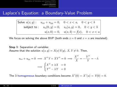
Laplace’s Equation: a Boundary-Value Problem
Solve u(x, y) : uxx + uyy = 0, 0 < x < a, 0 < y < bsubject to : ux(0, y) = 0, ux(a, y) = 0, 0 < y < b
u(x, 0) = 0, u(x, b) = f(x), 0 < x < a
We focus on solving the above BVP (both ends x = 0 and x = a are insulated).
Step 1: Separation of variables:Assume that the solution u(x, y) = X(x)Y(y), X,Y ̸= 0. Then,
uxx + uyy = 0 =⇒ X ′′Y + XY ′′ = 0 =⇒ X ′′
X = −Y ′′
Y = −λ
=⇒{
X ′′ + λX = 0
Y ′′ − λY = 0
The 3 homogeneous boundary conditions become X ′(0) = X ′(a) = Y(0) = 0.
34 / 50 王奕翔 DE Lecture 14
Separation of Variables and Classical PDE’sWave Equation
Laplace’s EquationSummary
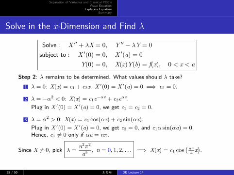
Solve in the x-Dimension and Find λ
Solve : X ′′ + λX = 0, Y ′′ − λY = 0
subject to : X ′(0) = 0, X ′(a) = 0
Y(0) = 0, X(x)Y(b) = f(x), 0 < x < a
Step 2: λ remains to be determined. What values should λ take?1 λ = 0: X(x) = c1 + c2x. X ′(0) = X ′(a) = 0 =⇒ c2 = 0.
2 λ = −α2 < 0: X(x) = c1e−αx + c2eαx.Plug in X ′(0) = X ′(a) = 0, we get c1 = c2 = 0.
3 λ = α2 > 0: X(x) = c1 cos(αx) + c2 sin(αx).Plug in X ′(0) = X ′(a) = 0, we get c2 = 0, and c1α sin(αa) = 0.Hence, c1 ̸= 0 only if αa = nπ.
Since X ̸= 0, pick λ =n2π2
a2, n = 0, 1, 2, . . . =⇒ X(x) = c1 cos
( nπa x
).
35 / 50 王奕翔 DE Lecture 14
Separation of Variables and Classical PDE’sWave Equation
Laplace’s EquationSummary
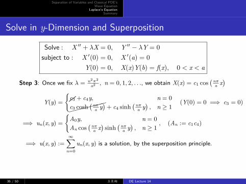
Solve in y-Dimension and Superposition
Solve : X ′′ + λX = 0, Y ′′ − λY = 0
subject to : X ′(0) = 0, X ′(a) = 0
Y(0) = 0, X(x)Y(b) = f(x), 0 < x < a
Step 3: Once we fix λ = n2π2
a2 , n = 0, 1, 2, . . ., we obtain X(x) = c1 cos( nπ
a x)
Y(y) ={��c3 + c4y, n = 0
������c3 cosh( nπ
a y)+ c4 sinh
( nπa y
), n ≥ 1
(Y(0) = 0 =⇒ c3 = 0)
=⇒ un(x, y) ={
A0y, n = 0
An cos( nπ
a x)
sinh( nπ
a y), n ≥ 1
, (An := c1c4)
=⇒ u(x, y) :=∞∑
n=0
un(x, y) is a solution, by the superposition principle.
36 / 50 王奕翔 DE Lecture 14
Separation of Variables and Classical PDE’sWave Equation
Laplace’s EquationSummary
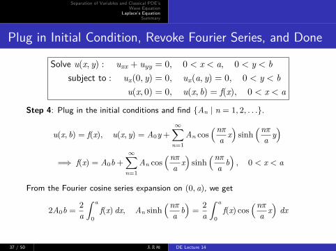
Plug in Initial Condition, Revoke Fourier Series, and Done
Solve u(x, y) : uxx + uyy = 0, 0 < x < a, 0 < y < bsubject to : ux(0, y) = 0, ux(a, y) = 0, 0 < y < b
u(x, 0) = 0, u(x, b) = f(x), 0 < x < a
Step 4: Plug in the initial conditions and find {An | n = 1, 2, . . .}.
u(x, b) = f(x), u(x, y) = A0y +
∞∑n=1
An cos(nπ
a x)
sinh(nπ
a y)
=⇒ f(x) = A0b +
∞∑n=1
An cos(nπ
a x)
sinh(nπ
a b), 0 < x < a
From the Fourier cosine series expansion on (0, a), we get
2A0b =2
a
∫ a
0
f(x) dx, An sinh(nπ
a b)=
2
a
∫ a
0
f(x) cos(nπ
a x)
dx
37 / 50 王奕翔 DE Lecture 14
Separation of Variables and Classical PDE’sWave Equation
Laplace’s EquationSummary
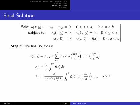
Final Solution
Solve u(x, y) : uxx + uyy = 0, 0 < x < a, 0 < y < bsubject to : ux(0, y) = 0, ux(a, y) = 0, 0 < y < b
u(x, 0) = 0, u(x, b) = f(x), 0 < x < a
Step 5: The final solution is
u(x, y) = A0y +
∞∑n=1
An cos(nπ
a x)
sinh(nπ
a y)
A0 =1
ab
∫ a
0
f(x) dx
An =2
a sinh(nπ
a b) ∫ a
0
f(x) cos(nπ
a x)
dx, n ≥ 1
38 / 50 王奕翔 DE Lecture 14
Separation of Variables and Classical PDE’sWave Equation
Laplace’s EquationSummary
Superposition Principle
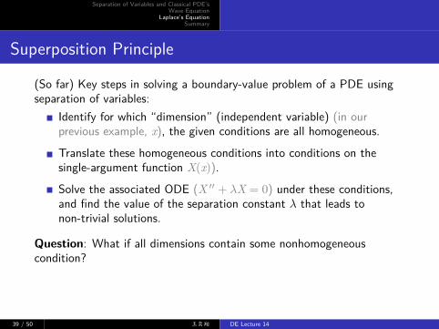
(So far) Key steps in solving a boundary-value problem of a PDE usingseparation of variables:
Identify for which “dimension” (independent variable) (in ourprevious example, x), the given conditions are all homogeneous.Translate these homogeneous conditions into conditions on thesingle-argument function X(x)).Solve the associated ODE (X ′′ + λX = 0) under these conditions,and find the value of the separation constant λ that leads tonon-trivial solutions.
Question: What if all dimensions contain some nonhomogeneouscondition?
39 / 50 王奕翔 DE Lecture 14
Separation of Variables and Classical PDE’sWave Equation
Laplace’s EquationSummary
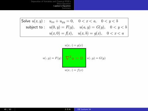
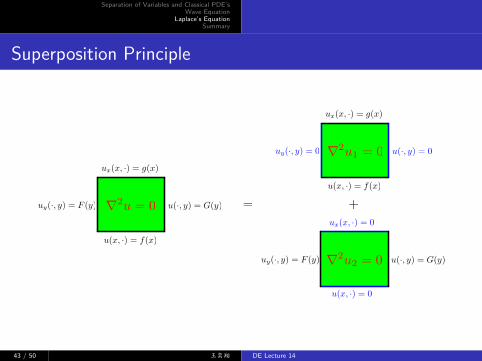
Solve u(x, y) : uxx + uyy = 0, 0 < x < a, 0 < y < bsubject to : u(0, y) = F(y), u(a, y) = G(y), 0 < y < b
u(x, 0) = f(x), u(x, b) = g(x), 0 < x < a
u(·, y) = F (y) u(·, y) = G(y)
u(x, ·) = f(x)
u(x, ·) = g(x)
r2u = 0
40 / 50 王奕翔 DE Lecture 14
Separation of Variables and Classical PDE’sWave Equation
Laplace’s EquationSummary
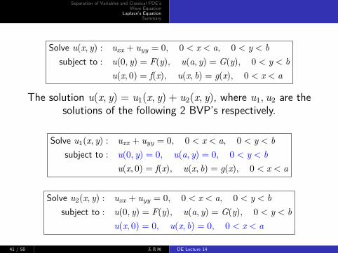
Solve u(x, y) : uxx + uyy = 0, 0 < x < a, 0 < y < bsubject to : u(0, y) = F(y), u(a, y) = G(y), 0 < y < b
u(x, 0) = f(x), u(x, b) = g(x), 0 < x < a
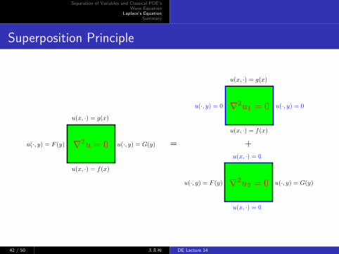
The solution u(x, y) = u1(x, y) + u2(x, y), where u1, u2 are thesolutions of the following 2 BVP’s respectively.
Solve u1(x, y) : uxx + uyy = 0, 0 < x < a, 0 < y < bsubject to : u(0, y) = 0, u(a, y) = 0, 0 < y < b
u(x, 0) = f(x), u(x, b) = g(x), 0 < x < a
Solve u2(x, y) : uxx + uyy = 0, 0 < x < a, 0 < y < bsubject to : u(0, y) = F(y), u(a, y) = G(y), 0 < y < b
u(x, 0) = 0, u(x, b) = 0, 0 < x < a
41 / 50 王奕翔 DE Lecture 14
Separation of Variables and Classical PDE’sWave Equation
Laplace’s EquationSummary
Superposition Principle
u(·, y) = F (y) u(·, y) = G(y)
u(x, ·) = f(x)
u(x, ·) = g(x)
u(x, ·) = f(x)
u(x, ·) = g(x)
u(·, y) = 0 u(·, y) = 0
u(·, y) = F (y) u(·, y) = G(y)
u(x, ·) = 0
u(x, ·) = 0
+r2u = 0
r2u1 = 0
r2u2 = 0
=
42 / 50 王奕翔 DE Lecture 14
Separation of Variables and Classical PDE’sWave Equation
Laplace’s EquationSummary
Superposition Principle
u(·, y) = 0
uy(·, y) = F (y) u(·, y) = G(y)
u(x, ·) = f(x)
u
x
(x, ·) = g(x)
u(x, ·) = f(x)
u
x
(x, ·) = g(x)
uy(·, y) = 0
uy(·, y) = F (y) u(·, y) = G(y)
u
x
(x, ·) = 0
+r2u = 0
r2u1 = 0
r2u2 = 0
=
u(x, ·) = 0
43 / 50 王奕翔 DE Lecture 14
Separation of Variables and Classical PDE’sWave Equation
Laplace’s EquationSummary
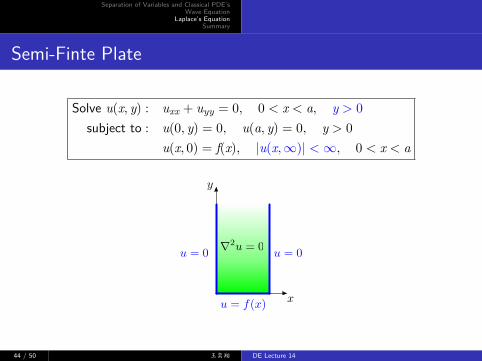
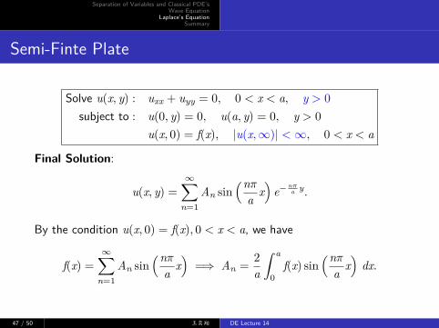
Semi-Finte Plate
Solve u(x, y) : uxx + uyy = 0, 0 < x < a, y > 0
subject to : u(0, y) = 0, u(a, y) = 0, y > 0
u(x, 0) = f(x), |u(x,∞)| < ∞, 0 < x < a
x
u = 0
u = f(x)
y
r2u = 0u = 0
44 / 50 王奕翔 DE Lecture 14
Separation of Variables and Classical PDE’sWave Equation
Laplace’s EquationSummary
Semi-Finte Plate
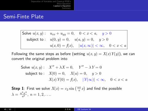
Solve u(x, y) : uxx + uyy = 0, 0 < x < a, y > 0
subject to : u(0, y) = 0, u(a, y) = 0, y > 0
u(x, 0) = f(x), |u(x,∞)| < ∞, 0 < x < a
Following the same steps as before (setting u(x, y) = X(x)Y(y)), we canconvert the original problem into
Solve u(x, y) : X ′′ + λX = 0, Y ′′ − λY = 0
subject to : X(0) = 0, X(a) = 0, y > 0
X(x)Y(0) = f(x), |Y(∞)| < ∞, 0 < x < a
Step 1: First we solve X(x) = c2 sin(nπ
a x)
and find the possibleλ = n2π2
a2 , n = 1, 2, . . ..
45 / 50 王奕翔 DE Lecture 14
Separation of Variables and Classical PDE’sWave Equation
Laplace’s EquationSummary
Semi-Finte Plate
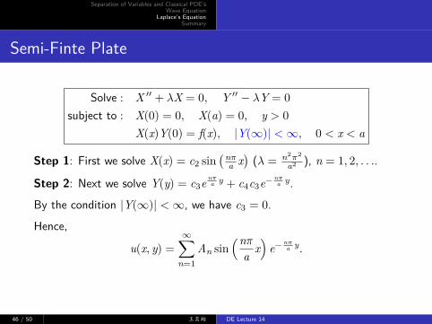
Solve : X ′′ + λX = 0, Y ′′ − λY = 0
subject to : X(0) = 0, X(a) = 0, y > 0
X(x)Y(0) = f(x), |Y(∞)| < ∞, 0 < x < a
Step 1: First we solve X(x) = c2 sin(nπ
a x)
(λ = n2π2
a2 ), n = 1, 2, . . ..
Step 2: Next we solve Y(y) = c3e nπa y + c4c3e− nπ
a y.By the condition |Y(∞)| < ∞, we have c3 = 0.Hence,
u(x, y) =∞∑
n=1
An sin(nπ
a x)
e− nπa y.
46 / 50 王奕翔 DE Lecture 14
Separation of Variables and Classical PDE’sWave Equation
Laplace’s EquationSummary
Semi-Finte Plate
Solve u(x, y) : uxx + uyy = 0, 0 < x < a, y > 0
subject to : u(0, y) = 0, u(a, y) = 0, y > 0
u(x, 0) = f(x), |u(x,∞)| < ∞, 0 < x < a
Final Solution:
u(x, y) =∞∑
n=1
An sin(nπ
a x)
e− nπa y.
By the condition u(x, 0) = f(x), 0 < x < a, we have
f(x) =∞∑
n=1
An sin(nπ
a x)
=⇒ An =2
a
∫ a
0
f(x) sin(nπ
a x)
dx.
47 / 50 王奕翔 DE Lecture 14
Separation of Variables and Classical PDE’sWave Equation
Laplace’s EquationSummary
1 Separation of Variables and Classical PDE’s
2 Wave Equation
3 Laplace’s Equation
4 Summary
48 / 50 王奕翔 DE Lecture 14
Separation of Variables and Classical PDE’sWave Equation
Laplace’s EquationSummary
Short Recap
Method of Separation of Variables: Convert PDE into two ODE’s
Solve the ODE with homogeneous boundary conditions first, todetermine the separation constant
Fourier Series to determine the undetermined coefficients
Heat Equation, Wave Equation, Laplace’s Equation
Superposition Principle
49 / 50 王奕翔 DE Lecture 14
Separation of Variables and Classical PDE’sWave Equation
Laplace’s EquationSummary
Self-Practice Exercises
12-1: 9, 15, 17, 22
12-2: 1, 3, 7, 11
12-4: 3, 7, 9, 11, 14
12-5: 5, 7, 12, 15, 19
50 / 50 王奕翔 DE Lecture 14