chapter 11 probabilistic approaches to ecg …gari/ecgbook/ch11.pdf · this rhythm can degenerate...

P1: Shashi

August 24, 2006 11:53 Chan-Horizon Azuaje˙Book

C H A P T E R 11

Probabilistic Approaches to ECGSegmentation and Feature Extraction

Nicholas P. Hughes

11.1 Introduction

The development of new drugs by the pharmaceutical industry is a costly and lengthyprocess, with the time from concept to final product typically lasting 10 years.Perhaps the most critical stage of this process is the phase one study, where thedrug is administered to humans for the first time. During this stage each subjectis carefully monitored for any unexpected adverse effects which may be broughtabout by the drug. Of particular interest is the ECG of the patient, which providesdetailed information about the state of the patient’s heart.

By examining the ECG signal in detail, it is possible to derive a number of in-formative measurements from the characteristic ECG waveform. These can then beused to assess the medical well-being of the patient, and more importantly, detectany potential side effects of the drug on the cardiac rhythm. The most importantof these measurements is the QT interval. In particular, drug-induced prolongationof the QT interval (so called Long QT Syndrome) can result in a very fast, abnor-mal heart rhythm known as torsade de pointes. This rhythm can degenerate intoventricular fibrillation and hence lead to sudden cardiac death.

In practice, QT interval measurements are carried out manually by speciallytrained ECG analysts. This is an expensive and time-consuming process, which issusceptible to mistakes by the analysts and provides no associated degree of confi-dence (or accuracy) in the measurements. This problem was recently highlighted inthe case of the antihistamine terfenadine, which had the side effect of significantlyprolonging the QT interval in a number of patients. Unfortunately this side effectwas not detected in the clinical trials and only came to light after a large number ofpeople had unexpectedly died while taking the drug [1].

In this chapter we consider the problem of automated ECG interval analysisfrom a probabilistic modeling perspective. In particular, we examine the use of hid-den Markov models for automatically segmenting an ECG signal into its constituentwaveform features. An undecimated wavelet transform is used to provide an infor-mative representation which is both robust to noise and tuned to the morphologicalcharacteristics of the waveform features. Finally we investigate the use of durationconstraints for improving the robustness of the model segmentations.

291

P1: Shashi


292 Probabilistic Approaches to ECG Segmentation and Feature Extraction

11.2 The Electrocardiogram

11.2.1 The ECG Waveform

Each individual heartbeat is comprised of a number of distinct cardiological stages,which in turn give rise to a set of distinct features in the ECG waveform. These fea-tures represent either depolarization (electrical discharging) or repolarization (elec-trical recharging) of the muscle cells in particular regions of the heart.Figure 11.1 shows a human ECG waveform and the associated features. The stan-dard features of the ECG waveform are the P wave, the QRS complex, and the Twave. Additionally a small U wave (following the T wave) is occasionally present.

The cardiac cycle begins with the P wave (the start and end points of whichare referred to as Pon and Poff), which corresponds to the period of atrial depolar-ization in the heart. This is followed by the QRS complex, which is generally themost recognizable feature of an ECG waveform, and corresponds to the period ofventricular depolarization. The start and end points of the QRS complex arereferred to as the Q and J points. The T wave follows the QRS complex and corre-sponds to the period of ventricular repolarization. The end point of the T wave is re-ferred to as Toff and represents the end of the cardiac cycle (presuming the absence ofa U wave).

11.2.2 ECG Interval Analysis

The timing between the onset and offset of particular features of the ECG (referredto as an interval) is of great importance since it provides a measure of the state ofthe heart and can indicate the presence of certain cardiological conditions. Two of

Figure 11.1 A typical human ECG waveform and its associated feature boundaries.

P1: Shashi


11.3 Automated ECG Interval Analysis 293

the most important intervals in the ECG waveform are the QT interval and the PRinterval. The QT interval is defined as the time from the start of the QRS complex tothe end of the T wave (i.e., Toff−Q) and corresponds to the total duration of electricalactivity (both depolarization and repolarization) in the ventricles. Similarly, the PRinterval is defined as the time from the start of the P wave to the start of theQRS complex (i.e., Q−Pon) and corresponds to the time from the onset of atrialdepolarization to the onset of ventricular depolarization.

Changes in the QT interval are currently the gold standard for evaluating theeffects of drugs on ventricular repolarization. In addition, changes in the PR intervalcan indicate the presence of specific cardiological conditions such as atrioventric-ular block [2]. Thus, the accurate measurement and assessment of the QT and PRintervals is of paramount importance in clinical drug trials.

11.2.3 Manual ECG Interval Analysis

Manual ECG interval analysis is typically performed by specialist ECG analysiscompanies known as centralized ECG core laboratories. The expert analysts (or“readers”) employed by these labs are generally a mixture of professional cardiol-ogists and highly trained cardiac technicians.

The accurate measurement of the QT interval is made difficult by the need tolocate the end of the T wave to a high level of precision. In theory, the end of theT wave is defined as the point at which the ECG signal (for the T wave) returnsto the isoelectric baseline. In practice, however, determining this point precisely ischallenging due to the variation in the baseline amplitude, unusual or abnormal Twave morphologies (such as T-U fusions or flat T waves), and the presence of noiseor artifact in the signal.

As a result, T wave offset measurements by expert analysts are inherently sub-jective and the associated QT interval measurements often suffer from a high degreeof interanalyst and intra-analyst variability. There has therefore been much focus onthe problem of developing an automated ECG interval analysis system, which couldprovide robust and consistent measurements, together with an associated degree ofconfidence in each measurement [3].

11.3 Automated ECG Interval Analysis

Standard approaches to ECG segmentation attempt to find the ECG waveformfeature boundaries from a given ECG signal in a number of successive stages [4]. Inthe first stage, a standard QRS detection algorithm (such as the Pan and Tompkinsalgorithm [5]) is used to locate the R peaks in the ECG signal. Given the locationof the R peak in each ECG beat, the next stage in the process is to search forwardsand backwards from this point to estimate the locations of the onset and offsetboundaries for the various ECG features [4].

In common with manual analysis, the accurate determination of the end of the Twave with automated methods is a challenging problem. The standard approach tothis problem is based on the tangent method, which is illustrated in Figure 11.2. Thistechnique, which was first introduced in 1952, locates the end of the T wave as the

P1: Shashi



Figure 11.2 An example of the tangent method for determining the end of the T wave. A tangentto the T wave is computed at the point of maximum (absolute) gradient following the T wave peak,and the intersection of this tangent with the estimated isoelectric baseline gives the T wave offsetlocation.

point of intersection between the (estimated) isoelectric baseline and the tangent tothe downslope of the T wave (or the upslope for inverted T waves) [6]. The tangentitself is computed at the point of maximum (absolute) gradient following the peakof the T wave.

A significant disadvantage of the tangent method is that it is sensitive to theamplitude of the T wave. In particular, large amplitude T waves can cause thetangent to intersect the isoelectric baseline well before the actual end of the T wave.As a result, the automated QT intervals from the tangent method can significantlyunderestimate the actual QT interval value. To overcome this problem, Xu andReddy applied a “nonlinear correction” factor (based on the T wave amplitude) tothe T wave offset determined by the tangent method [7].

In practice, automated QT interval measurements continue to be unreliable inthe presence of noisy waveforms or unusual T wave morphologies. In addition, it isstill the case that automated systems can produce highly unreliable measurementsfor relatively clean ECGs with regular waveform morphologies [8]. As a result, ECGinterval measurements for clinical drug trials are generally performed manually byhuman experts.

11.4 The Probabilistic Modeling Approach

The probabilistic modeling approach to automated ECG interval analysis offers anumber of significant advantages compared with traditional approaches. In partic-ular, probabilistic models provide the following benefits:

P1: Shashi


11.4 The Probabilistic Modeling Approach 295

• The ability to learn from ECG data sets annotated by human experts;• The ability to incorporate prior knowledge about the statistical characteristics

of the ECG waveform features in a principled manner;• The ability to produce confidence measures in the automated ECG interval

measurements.

One of the most powerful features of the probabilistic modeling approach isthe ability to learn a model for ECG segmentation from expert annotated ECGdata. Such data-driven learning allows us to sidestep neatly the problem of havingto specify an explicit rule for determining the end of the T wave in the electro-cardiogram (e.g., the tangent method). Since rule-based approaches are inherentlyunreliable for this particular problem (given the wide range of ECG morphologieswhich can occur in practice), it is much more appropriate to learn the statisticalcharacteristics which define the ECG waveform feature boundaries using measure-ments from expert analysts. Furthermore, this learning approach enables us to buildmodels from ECG data sets which exhibit specific types of waveform morphologies,or from those corresponding to specific patient cohorts [9].

The most appropriate form of probabilistic model to apply to the task of au-tomated ECG interval analysis is a hidden Markov model (HMM). These modelscan be viewed as a form of state space model. Specifically, HMMs make use of adiscrete state space to capture the sequential characteristics of the data. This par-ticular formulation offers an attractive framework for ECG signal modeling, sinceit allows each of the ECG waveform features (i.e., P wave, QRS complex, T wave,and so forth) to be uniquely associated with a particular state in the model. Thus,the model is able to take advantage of the sequence ordering which exists betweenthe different waveform features of normal ECGs.

An additional advantage of utilizing hidden Markov models when consideringprobabilistic approaches to ECG segmentation is that there are efficient algorithmsfor HMM training and testing. Specifically, the parameters of an HMM can beestimated straightforwardly in a supervised manner using a data set of ECG wave-forms together with the corresponding expert measurements of the waveform fea-ture boundaries. Alternatively, if the data set contains only the ECG waveforms(i.e., the associated expert measurements are unavailable), then the EM algorithmcan be used to train the model in an unsupervised manner [10]. Once the model hasbeen trained, the Viterbi algorithm can be used to segment test ECG signals.

A disadvantage of the probabilistic modeling approach is that the segmentationof ECGs typically requires more computing power (for the same level of processingperformance) compared with standard algorithms. For the analysis of 10-second12-lead ECG signals, this is rarely an issue. However, when very large amountsof ECG data must be processed rapidly (e.g., for the analysis of continuous 12-lead digital Holter recordings), it may be necessary to combine both standard(nonprobabilistic) and probabilistic algorithms to achieve an appropriate rate ofsegmentation.

Although the use of hidden Markov models for ECG analysis has been consid-ered previously in the literature [11, 12], many of the issues involved in achieving ahigh level of segmentation accuracy with these models have not previously been dis-cussed in detail. In this chapter, we focus on the core issues which must be addressed

P1: Shashi



when using probabilistic models for automated ECG interval analysis. Specifically,we consider the choice of representation for the ECG signal, and the choice of modelarchitecture for the segmentation.

In the following sections, we describe how wavelet methods (and in particular,the undecimated wavelet transform) can be used to provide an encoding of the ECGwhich is more appropriate for subsequent modeling with HMMs. In addition, wedescribe how “duration constraints” can be incorporated into the HMM frameworksuch that the resulting model provides a more appropriate statistical descriptionof the normal ECG waveform, and hence a greater degree of robustness in thewaveform segmentations.

11.5 Data Collection

In order to develop an automated system for ECG interval analysis, we collecteda data set of over 100 ECG waveforms (sampled at 500 Hz), together with thecorresponding waveform feature boundaries as determined by a group of expertECG analysts. Due to time constraints it was not possible for each expert analystto label every ECG waveform in the data set. Therefore, we chose to distribute thewaveforms at random among the different experts (such that each waveform wasmeasured by one expert only).

For each ECG waveform, the following points were annotated: Pon, Poff, Q, J,and Toff (if a U wave was present, the Uoff point was also annotated). In addition, thepoint corresponding to the start of the next P wave (i.e., the P wave of the followingheartbeat), NPon, was also annotated. During the data collection exercise, we foundthat it was not possible to obtain reliable estimates for the Ton and Uon points, andtherefore these were taken to be the J and Toff points, respectively.

11.6 Introduction to Hidden Markov Modeling

11.6.1 Overview

Since their development in the late 1960s and early 1970s, hidden Markov modelshave proved to be a powerful and flexible class of statistical model for describingmany different kinds of sequential data. The term “sequential” here refers to thefact that there exists a natural ordering inherent in the data itself. This property isparticularly true of time-series data, where the individual data samples are orderedaccording to the particular time point at which they were measured. By incorpo-rating this sequence information into the structure of our model, we can ensurethat the model provides a good description of the data and its associated statisticalproperties.

The utility of hidden Markov models stems from the fact that they offer an ef-fective balance between the core data modeling issues of complexity and tractability.In particular, hidden Markov models are “rich” enough to provide a good statisticaldescription of many different kinds of sequence data, yet they are also sufficientlysimple as to admit efficient algorithms for inference and learning. This trade-offbetween descriptive modeling power and practical ease of use is perhaps the mainreason for the success of hidden Markov models in practice.

P1: Shashi


11.6 Introduction to Hidden Markov Modeling 297

This section presents a thorough review of hidden Markov models and theirassociated algorithms for inference and learning. We begin with a brief descriptionof Markov models in the context of stochastic processes, and then proceed to coverthe topic of hidden Markov models in more depth.

11.6.2 Stochastic Processes and Markov Models

A natural way to describe a stochastic process is in terms of the probability dis-tribution of the random variable under consideration. In particular, for processesthat evolve through time, it is often useful to consider a conditional probabilitydistribution of the form

p(xt | xt1 , xt2 , xt3 , . . .) (11.1)

which defines the probability of obtaining a sample value x at time t given a historyof previous values. If this distribution is time-invariant, such that it is only dependenton the time differences (or “lags”) and not the absolute time values, then the processis said to be strictly stationary.1 In this case, (11.1) can be written in the form:

p(xt | xt−τ1 , xt−τ2 , xt−τ3 , . . .) (11.2)

A special case of interest occurs when this conditional distribution is dependenton only a finite history of previous values, such that:

p(xt | xt−τ1 , xt−τ2 , . . . , xt−τN) (11.3)

which defines an Nth-order Markov process. If we now make the further simpli-fying assumption that the process depends soley on the previous value, then theconditional distribution becomes

p(xt | xt−τ ) (11.4)

This equation defines a first-order Markov process, which is often referred tosimply as a “Markov process” [13]. When dealing with a discrete-time discrete-valued random variable st, this Markov process becomes a Markov chain, with thecorresponding conditional distribution:

P(st | st−1) (11.5)

A Markov model can be used to represent any random variable st which canoccupy one of K possible discrete “states” at each time step and which satisfies theMarkov property

P(st+1 | st, st−1, st−2, . . .) = P(st+1 | st) (11.6)

Equation (11.6) captures the notion that “the future is conditionally indepen-dent of the past given the present.” Thus when evaluating the probability of the

1. A more relaxed definition of stationarity requires that only the first and second moments of the distributionare time-invariant, in which case the process is said to be weakly stationary.

P1: Shashi



system state at a particular time step, we need only consider the state at the previ-ous time step. Statistical models which exploit this Markov property often admitefficient algorithms for computing many practical quantities of interest.

In practice, a Markov model is governed by two distinct parameters: an ini-tial state distribution and a state transition matrix. The initial state distribution π

defines the probabilities of the random variable being in each of the K possible statesat the first time step (i.e., t = 1). Thus, this parameter is simply a K-dimensionalvector, where each element πk gives the corresponding probability P(s1 = k). Thestate transition matrix A defines the probability of the model “transitioning” to aparticular state at the next time step, given its state at the current time step. Thus,this parameter is a K × K matrix, where each element ai j gives the correspondingprobability P(st+1 = j | st = i). If it is possible to transition from any state to anyother state (i.e., ai j �= 0 ∀ i, j), then the model is said to be ergodic [7].

11.6.3 Hidden Markov Models

A hidden Markov model is a probabilistic model which describes the statisticalrelationship between an observable sequence O and an unobservable or “hidden”state sequence S. The hidden state itself is discrete and governed by an underly-ing Markov model. The observation values however may be either continuous ordiscrete in nature.

The key aspect of an HMM is that each observation value is considered to be theresult of an additional stochastic process associated with one of the hidden states.Thus, a hidden Markov model can be viewed as a “doubly embedded stochasticprocess with an underlying stochastic process that is not observable (it is hidden),but can only be observed through another set of stochastic processes that producethe sequence of observations” [10].

More formally, an HMM (with K hidden states) is defined by the followingthree parameters [10]:

• An initial state distribution π ;• A state transition matrix A;• An observation probability distribution bk for each state k.

The first two parameters govern the underlying Markov model which describesthe statistical properties of the hidden states. It is the observation probabilitydistributions2 however which differentiate a hidden Markov model from a stan-dard Markov model. More precisely, the observation probability distribution for agiven state models the probability of a particular observation value when the modeloccupies that particular state.

It is often useful to consider a hidden Markov model from a generative per-spective. That is, we can consider the HMM as providing a bottom-up descriptionof how the observed sequence O is produced or generated. Viewed as a generativemodel, the operation of an HMM is as follows:

2. The observation probability distributions are also known as emission probability distributions.

P1: Shashi



1. Select the initial state k by sampling from the initial state distribution π .2. Generate a observation value from this state by sampling from the associated

observation distribution bk.3. Select the state at the next time step based upon the transition matrix A.4. Return to step 2.

In the standard formulation of a hidden Markov model, the observation values“within” a given state are considered to be independent and identically distributed(i.i.d.). Hence, when an observation value is generated by a particular state at agiven time step, it is generated independently of any previous samples which mayhave been generated from that same state in previous time steps. Thus, conditionedon the state sequence, we can express the likelihood of a sequence of observationsas

p(O1:T | S1:T , λ) =T∏

t=1

p(Ot | St , λ) (11.7)

where λ represents the set of model parameters for the HMM. It is important torecognize that the factorization shown in (11.7) holds only when the observationsare conditioned on the state sequence. Thus, without knowledge of the underlyingstate sequence, we cannot make any independence assumptions about the proba-bility distribution of the observations [i.e., p(O1:T | λ)].

The assumption of statistical independence between successive observations(within a state) is perhaps the greatest weakness of the standard hidden Markovmodel. The validity of this assumption in the context of ECG signal modeling isconsidered in greater detail in Section 11.7.4.

Figure 11.3 shows two different graphical representations of a simple two-state hidden Markov model. The first representation, illustrated in Figure 11.3(a),shows the “architectural” view of an HMM. This form of the model highlights theoverall HMM topology together with the role of the individual model parameters.In particular, the two clear nodes correspond to the two individual hidden states

Figure 11.3 Two different graphical representations of a hidden Markov model. (a) In the standardrepresentation the clear nodes corresponds to specific hidden states in the model, and the shadednodes correspond to the observations which are generated by those hidden states. (b) In the DBNrepresentation each clear node corresponds to the particular state which the model occupies ata given time step, and each shaded node corresponds to the associated observation generated bythat state.

P1: Shashi



Figure 11.4 Alternative ‘‘views’’ of a hidden Markov model. (a) The HMM as a simple Markovmodel in which the states are stochastically related to the observations. (b) The HMM as a formof temporal mixture model in which the individual mixture components obey a sequence ordering(governed by the transition matrix).

in the model, and the two shaded nodes correspond to the observations that aregenerated by those hidden states.

The second representation, illustrated in Figure 11.3(b), shows the HMM as adynamic Bayesian network (DBN) [14]. Here the HMM is shown “unrolled” overa number of time steps. Each clear node3 now corresponds to the particular statewhich the model occupies at a given time step, and each shaded node corresponds tothe associated observation generated by that state. Both graphical representationsserve to illustrate the role of an HMM as a statistical model for sequential data.

Hidden Markov models can also be seen as generalizations of various statisticalmodels [15, 16]. Figure 11.4 shows two such possible “views” of an HMM. Thefirst, shown in Figure 11.4(a), denotes the HMM as a simple Markov model withstochastic observations. This is the view outlined previously in this section. Analternative perspective, however, can be gained by considering the HMM as a formof temporal mixture model, as illustrated in Figure 11.4(b). With a standard (static)mixture model, each data point is considered to have been “generated” by one of theK mixture components independently of the other data points [17]. If we now relaxthe strong assumption of statistical independence between data points and allowthe individual mixture components to possess Markovian “dynamics,” the result isa hidden Markov model (where the hidden state at each time step corresponds tothe particular mixture component which is active at that time step).

More generally, hidden Markov models can be viewed under the general frame-work of probabilistic graphical models [18]. Such models include standard “state-space” models such as hidden Markov models and Kalman filters as special cases,as well as more advanced models such as coupled HMMs [19] and factorialHMMs [20].

From a purely statistical perspective, an HMM defines a joint probability distri-bution over observation sequences Oand hidden state sequences S [i.e., p(O, S | λ)].Given this joint distribution, it is often of interest to find the particular state sequencewhich maximizes the conditional distribution P(S | O, λ). This corresponds to

3. In the “language” of Bayesian networks, a square node represents a discrete value and a circular noderepresents a continuous value. Similarly a clear node represents a hidden (or latent) variable and a shadednode represents an observed variable. Hence in Figure 11.3(b), the hidden states are shown as clear squarenodes, and the observations (which are assumed to be continuous in this example) are shows as shadedcircular nodes.

P1: Shashi



the state sequence which is most likely to have “generated” the given observationsequence, and thus provides an effective means to segment the observation sequenceinto its characteristic features. However, before we can use an HMM for such pur-poses, we must first learn the “optimal” parameters of the model from a given dataset (such that the HMM provides a useful statistical model of the data). We nowconsider the solution to each of these problems in greater detail.

11.6.4 Inference in HMMs

The inference problem for hidden Markov models is typically cast as the problemof determining the single most probable state sequence given the observation data,that is,

S∗ = argmaxS

{P(S | O, λ)} (11.8)

This can be reexpressed using Bayes’ rule as

S∗ = argmaxS

{P (S | O, λ)}

= argmaxS

{p (S, O | λ)

p(O | λ)

}= argmax

S{p (S, O | λ)} (11.9)

Hence it suffices to find the state sequence S∗ which maximizes the joint dis-tribution p(S, O | λ). The solution to this problem is known as the Viterbi al-gorithm [21, 22]. More precisely, the Viterbi algorithm is a dynamic program-ming procedure which takes advantage of the Markov property of the HMM statesequence.

To apply dynamic programming to the HMM inference problem, we must firstdefine the variable δt(i):

δt(i) = maxs1s2···st−1

{p(s1s2 · · · st = i, O1O2 · · · Ot | λ)} (11.10)

This is the likelihood of the most probable state sequence that accounts for thefirst t observations and ends in state i at time t. Now consider computing the valueof the delta variable at the next time step t + 1. We can express this computation as

δt+1(i) = maxs1s2···st

{p(s1s2 · · · st+1 = i, O1O2 · · · Ot+1 | λ)

}= max

j

{max

s1s2···st−1

{p(s1s2 · · · st = j, O1O2 · · · Ot | λ)

}×P(st+1 = i | st = j)

}p(Ot+1 | st+1 = i)

= maxj

{δt( j) a ji

}bi (Ot+1) (11.11)

The key step in developing the recurrence relation for δt+1(i) is to note thatwe can make use of the solutions to the previous subproblems at time step t.

P1: Shashi



In particular, we can compute the most probable state sequence that accounts forthe first t + 1 observations and ends in state i by maximizing over the K previoussolutions [i.e., δt( j)] and the appropriate transition probability (a ji ).

The recursion is initialized for each state i by computing the probability of themodel occupying state i at the first time step and producing the first observationvalue O1 from that particular state, that is,

δ1(i) = πi bi (O1) (11.12)

Equation (11.11) can then be used to compute the value of δt(i) for each statei and for each time step from t = 2 to t = T. Following the final computation att = T, we have

δT(i) = maxs1s2···sT−1

{p(s1s2 · · · sT = i, O1O2 · · · OT | λ)} (11.13)

The optimal value for the hidden state at the final time step is then computedas the particular state which maximizes (11.13)

s∗T = argmax

i

{δT(i)

}(11.14)

Using this knowledge of the optimal state value at the final time step, we can then“work back” to uncover the optimal state value at the previous time step t = T −1.This is given by the particular state argument which maximized δT(s∗

T) as part ofits recursive computation. Based on this value, we can follow a similar procedureto uncover the optimal state value at time step T − 2. This general backtrackingprocedure can be performed successively to uncover the full optimal hidden statesequence S∗.

When computing (11.11) in practice, it is common to record the particular“maximizing” state which maximizes the value of δt+1(i):

ψt+1(i) = argmaxj

{δt( j) a ji

}(11.15)

The back-tracking procedure to uncover the optimal state sequence can then beimplemented as a look-up process using the stored ψ values:

s∗t = ψt+1(s∗

t+1) t = T − 1, T − 2, · · · , 1 (11.16)

Pseudo-code for the Viterbi procedure is shown in Listing 1. Note that in prac-tice, the implementation of the Viterbi algorithm requires the use of a simple “scal-ing” procedure to ensure that the δt(i) values do not under- or overflow [10].

11.6.5 Learning in HMMs

The learning problem in hidden Markov models is concerned with determiningthe optimal model parameters given a particular training data set. If the data setconsists of both the observation sequences and the corresponding hidden state se-quences (which generated the observation sequences), then the HMM parameter

P1: Shashi



Listing 1 Viterbi algorithm

//Initialization:for i = 1 to K

δ1(i) = πi bi (O1)ψ1(i) = 0

end

//Recursion:for t = 2 to T

//Compute delta at time t for each state i//and record “maximizing” predecessor statefor i = 1 to K

δt(i) = max{δt−1( j)a ji bi (Ot)}1≤ j≤K

ψt(i) = argmax{δt−1( j)a ji }1≤ j≤K

endend

//Termination:P∗ = max{δT(i)}

1≤ j≤K

s∗T = argmax{δT(i)}

1≤ j≤K

//Backtracking:for t = T − 1 to 1

s∗t = ψt+1(s∗

t+1)end

estimation problem can be viewed as a supervised learning problem. Conversely, ifthe data set consists of only the observation sequences, then the problem is one ofunsupervised learning. We now consider each of these two cases in turn.

11.6.5.1 Supervised Learning

In the supervised learning case, we can make use of both the observation sequencesand the corresponding hidden state sequences to derive simple estimates for themodel parameters. In particular, we can estimate the initial state distribution byevaluating the fraction of the hidden state sequences which commence in each ofthe given model states at the first time step. More precisely, denoting the totalnumber of hidden state sequences which commence in state i at the first time stepby ninit(i), then we have the following estimator for the ith element of the initialstate distribution:

πi = ninit(i)∑Kk=1 ninit(k)

(11.17)

In a similar manner, we can estimate the transition matrix by evaluating thefraction of particular state transitions over all the hidden state sequences. Moreprecisely, denoting the total number of transitions from state i to state j over allthe hidden state sequences by ntrans(i, j), then we have the following estimator forthe (i, j)th element of the transition matrix:

ai j = ntrans(i, j)∑Kk=1 ntrans(i, k)

(11.18)

P1: Shashi



The exact estimator for the parameters of the observation models depends on thespecific functional form chosen for these models. However, the general estimationprocedure for the observation models is straightforward. For each state i , we simply“extract” all the observations which correspond to that particular state (i.e., thosethat were “generated” by that state) and then fit the observation model to this datain a standard manner.

11.6.5.2 Unsupervised Learning

In the unsupervised learning case, we are provided with a data set of observationsequences only (i.e., we do not have access to the corresponding hidden state se-quences). This makes the learning procedure much more difficult compared withthe supervised case previously described.

Given the data set of observation sequences O = {O1, O2, . . . , O N}, the un-supervised learning problem is typically cast in a maximum likelihood framework.More precisely, we seek the model parameters λ∗ which maximize the probabilityof the data; that is,

λ∗ = argmax{

p (O | λ)}

(11.19)λ

Fortunately, there exists a particularly effective approach to solving (11.19) forhidden Markov models (and many other types of statistical models). This approachis known as the EM algorithm,4 and is a general method for unsupervised learningin the presence of “missing” or incomplete data [23].

We now discuss the application of hidden Markov models to the particularproblem of ECG segmentation.

11.7 Hidden Markov Models for ECG Segmentation

This section presents a detailed analysis of the use of hidden Markov models forsegmenting ECG signals. The general aim of any signal segmentation method is to“partition” a given signal into consecutive regions of interest. In the context of theECG then, the role of segmentation is to determine as accurately as possible theonset and offset boundaries of the various waveform features (e.g., P wave, QRScomplex, T wave, and so forth), such that the ECG interval measurements may becomputed automatically.

In Section 11.7.1, we discuss the different types of hidden Markov model archi-tecture which can be used for ECG segmentation. Following this, we discuss the twodifferent forms of segmentations which can occur when a trained HMM is used tosegment ECG signals in practice. The performance of HMMs for ECG segmentationis then considered in more detail. In particular, we examine a number of differentstate observation models, as well as the use of ECG signal normalization techniques.

4. In the context of hidden Markov models, the EM algorithm is often referred to as the Baum-Welch algorithm.

P1: Shashi


11.7 Hidden Markov Models for ECG Segmentation 305

11.7.1 Overview

The first step in applying hidden Markov models to the task of ECG segmenta-tion is to associate each state in the model with a particular region of the ECG. Asdiscussed previously in Section 11.6.5, this can either be achieved in a supervisedmanner (i.e., using expert measurements) or an unsupervised manner (i.e., usingthe EM algorithm). Although the former approach requires each ECG waveformin the training data set to be associated with expert measurements of the wave-form feature boundaries (i.e., the Pon, Q, Toff points, and so forth), the resultingmodels generally produce more accurate segmentation results compared with theirunsupervised counterparts.

Figure 11.5 shows a variety of different HMM architectures for ECG intervalanalysis. A simple way of associating each HMM state with a region of the ECG isto use individual hidden states to represent the P wave, QRS complex, JT intervaland baseline regions of the ECG, as shown in Figure 11.5(a). In practice, it isadvantageous to partition the single baseline state into multiple baseline states [9],one of which is used to model the baseline region between the end of the P waveand the start of the QRS complex (termed “baseline 1”), and another which is usedto model the baseline region following the end of the T wave (termed “baseline 2”).This model architecture, which is shown in Figure 11.5(b), will be used throughoutthe rest of this chapter.5

Following the choice of model architecture, the next step in training an HMM isto decide upon the specific type of observation model which will be used to capturethe statistical characteristics of the signal samples from each hidden state. Commonchoices for the observation models in an HMM are the Gaussian density, the Gaus-sian mixture model (GMM), and the autoregressive (AR) model. Section 11.7.4 dis-cusses the different types of observation models in the context of ECG segmentation.

Before training a hidden Markov model for ECG segmentation, it is beneficialto consider the use of preprocessing techniques for ECG signal normalization.

11.7.2 ECG Signal Normalization

In many pattern recognition tasks it is advantageous to normalize the raw input dataprior to any subsequent modeling [24]. A particularly simple and effective form ofsignal normalization is a linear rescaling of the signal sample values. In the case ofthe ECG, this procedure can help to normalize the dynamic range of the signal andto stabilize the baseline sections.

A useful form of signal normalization is given by range normalization, whichlinearly scales the signal samples such that the maximum sample value is set to +1and the minimum sample value to −1. This can be achieved in a simple two-stepprocess. First, the signal samples are “amplitude shifted” such that the minimumand maximum sample values are equidistant from zero. Next, the signal samplesare linearly scaled by dividing by the new maximum sample value. These two steps

5. Note that it is also possible to use an “optional” U wave state (following the T wave) to model any U wavesthat may be present in the data, as shown in Figure 11.5(c).

P1: Shashi



Figure 11.5 (a–e) Hidden Markov model architectures for ECG interval analysis.

can be stated mathematically as

x′n = xn −

(xmin + xmax

2

)(11.20)

and

yn = x′n

x′max

(11.21)

P1: Shashi



where xmin and xmax are the minimum and maximum values in the original signal,respectively. The range normalization procedure can be made more robust to thepresence of artefact or “spikes” in the ECG signal by computing the median of theminimum and maximum signal values over a number of different signal segments.Specifically, the ECG signal is divided evenly into a number of contiguous segments,and the minimum and maximum signal values within each segment are computed.The ECG signal is then range normalized (i.e., scaled) to the median of the minimumand maximum values over the given segments.

11.7.3 Types of Model Segmentations

Before considering in detail the results for HMMs applied to the task of ECGsegmentation, it is advantageous to consider first the different types of ECG seg-mentations that can occur in practice. In particular, we can identify two distinctforms of model segmentations when a trained HMM is used to segment a given10-second ECG signal:

• Single-beat segmentations: Here the model correctly infers only one heartbeatwhere there is only one beat present in a particular region of the ECG signal.

• Double-beat segmentations: Here the model incorrectly infers two or moreheartbeats where there is only one beat present in a particular region of theECG signal.

Figure 11.6(a, b) shows examples of single-beat and double-beat segmentations,respectively. In the example of the double-beat segmentation, the model incorrectlyinfers two separate beats in the ECG signal shown. The first beat correctly locatesthe QRS complex but incorrectly locates the end of the T wave (in the region ofbaseline prior to the T wave). The second beat then “locates” another QRS complex(of duration one sample) around the onset of the T wave, but correctly locates theend of the T wave in the ECG signal. The specific reason for the occurrence ofdouble-beat segmentations and a method to alleviate this problem are covered inSection 11.9.

In the case of a single-beat segmentation, the segmentation errors can be eval-uated by simply computing the discrepancy between each individual automatedannotation (e.g., Toff ) and the corresponding expert analyst annotation. In the caseof a double-beat segmentation, however, it is not possible to associate uniquelyeach expert annotation with a corresponding automated annotation. Given this, itis therefore not meaningful to attempt to evaluate a measure of annotation “error”for double-beat segmentations. Thus, a more informative approach is simply to re-port the percentage of single-beat segmentations for a given ECG data set, alongwith the segmentation errors for the single-beat segmentations only.

11.7.4 Performance Evaluation

The technique of cross-validation [24] was used to evaluate the performance ofa hidden Markov model for automated ECG segmentation. In particular, five-fold cross-validation was used. In the first stage, the data set of annotated ECG

P1: Shashi



Figure 11.6 Examples of the two different types of HMM segmentations which can occur in prac-tice: (a) single- and (b) double-beat segmentation.

waveforms was partitioned into five subsets of approximately equal size (in termsof the number of annotated ECG waveforms within each subset). For each “fold”of the cross-validation procedure, a model was trained in a supervised manner usingall the annotated ECG waveforms from four of the five subsets. The trained modelwas then tested on the data from the remaining subset. This procedure was repeatedfor each of the five possible test subsets. Prior to performing cross-validation, thecomplete data set of annotated ECG waveforms was randomly permuted in orderto remove any possible ordering which could affect the results.

As previously stated, for each fold of cross-validation a model was trainedin a supervised manner. The transition matrix was estimated from the trainingwaveform annotations using the supervised estimator given in (11.18). For Gaussianobservation models, the mean and variance of the full set of signal samples werecomputed for each model state. For Gaussian mixture models, a combined MDL

P1: Shashi



and EM algorithm was used to compute the optimal number of mixture componentsand the associated parameter values [25]. For autoregressive6 or AR models, theBurg algorithm [26] was used to infer the model parameters and the optimal modelorder was computed using an MDL criterion.

Following the model training for each fold of cross-validation, the trainedHMM was then used to segment each 10-second ECG signal in the test set. Thesegmentation was performed by using the Viterbi algorithm to infer the most prob-able underlying sequence of hidden states for the given signal. Note that the full10-second ECG signal was processed, as opposed to just the manually annotatedECG beat, in order to more closely match the way an automated system would beused for ECG interval analysis in practice.

Next, for each ECG, the model annotations corresponding to the particular beatwhich had been manually annotated were then extracted. In the case of a single-beat segmentation, the absolute differences between the model annotations andthe associated expert analyst annotations were computed. In the case of a double-beat segmentation, no annotation errors were computed. Once the cross-validationprocedure was complete, the five sets of annotation “errors” were then averaged toproduce the final results.

Table 11.1 shows the cross-validation results for HMMs trained on the raw ECGsignal data. In particular, the table shows the percentage of single-beat segmenta-tions and the annotation errors for different types of HMM observation modelsand with/without range normalization, for ECG leads II and V2.

The results for each lead demonstrate the utility of normalizing the ECG sig-nals (prior to training and testing) with the range normalization method. In eachcase, the percentage of single-beat segmentations produced by an HMM (with aGaussian observation model) is considerably increased when range normalizationis employed. For lead V2, it is notable that the annotation errors (evaluated onthe single-beat segmentations only) for the model with range normalization aregreater than those for the model with no normalization. This is most likely tobe due to the fact that the latter model produces double-beat segmentations forthose waveforms that naturally give rise to larger annotation errors (and hencethese waveforms are excluded from the annotation error computations for thismodel).

The most important aspect of the results is the considerable performance im-provement gained by using autoregressive observation models as opposed to Gaus-sian or Gaussian mixture models. The use of AR observation models enables eachHMM state to capture the statistical dependencies between successive groups ofobservations. In the case of the ECG, this allows the HMM to take account ofthe shape of each of the ECG waveform features. Thus, as expected, these modelslead to a significant performance improvement (in terms of both the percentage ofsingle-beat segmentations and the magnitude of the annotation errors) comparedwith models which assume the observations within each state are i.i.d.

6. In autoregressive modeling, the signal sample at time t is considered to be a linear combination of a numberof previous signal samples plus an additive noise term. Specifically, an AR model of order m is given byxt = ∑m

i=1 ci xt−i + εt, where ci are the AR model coefficients and εt can be viewed as a random residualnoise term at each time step.

P1: Shashi



Table 11.1 Five-Fold Cross-Validation Results for HMMs Trained on the Raw ECG SignalData from Leads II and V2

Lead IIHidden Markov Model % of Single-Beat Mean Absolute Errors (ms)Specification Segmentations Pon Q J Toff

Standard HMMGaussian observation model 5.7% 175.3 108.0 99.0 243.7No normalization

Standard HMMGaussian observation model 69.8% 485.0 35.8 73.8 338.4Range normalization

Standard HMMGMM observation model 57.5% 272.9 48.7 75.6 326.1Range normalization

Standard HMMAR observation model 71.7% 49.2 10.3 12.5 52.8Range normalization

Lead V2

Hidden Markov Model % of Single-Beat Mean Absolute Errors (ms)Specification Segmentations Pon Q J Toff

Standard HMMGaussian observation model 33.6% 211.5 14.5 20.7 31.5No normalization

Standard HMMGaussian observation model 77.9% 293.1 49.2 50.7 278.5Range normalization

Standard HMMGMM observation model 57.4% 255.2 49.9 65.0 249.5Range normalization

Standard HMMAR observation model 87.7% 43.4 5.4 7.6 32.4Range normalization

Despite the advantages offered by AR observation models, the mean annotationerrors for the associated HMMs are still considerably larger than the inter-analystvariability present in the data set annotations. In particular, the T wave offset anno-tation errors for leads II and V2 are 52.8 ms and 32.4 ms, respectively. This “levelof accuracy” is not sufficient to enable the trained model to be used as an effectivemeans for automated ECG interval analysis in practice.

The fundamental problem with developing HMMs based on the raw ECG signaldata is that the state observation models must be flexible enough to capture thestatistical characteristics governing the overall shape of each of the ECG waveformfeatures. Although AR observation models provide a first step in this direction,these models are not ideally suited to representing the waveform features of theECG. In particular, it is unlikely that a single AR model can successfully representthe statistical dependencies across whole waveform features for a range of ECGs.

P1: Shashi


11.8 Wavelet Encoding of the ECG 311

Thus, it may be advantageous to utilize multiple AR models (each with a separatemodel order) to represent the different regions of each ECG waveform feature.

An alternative approach to overcoming the i.i.d. assumption within each HMMstate is to encode information from “neighboring” signal samples into the rep-resentation of the signal itself. More precisely, each individual signal sample istransformed to a vector of transform coefficients which captures (approximately)the shape of the signal within a given region of the sample itself. This newrepresentation can then be used as the basis for training a hidden Markov model,using any of the standard observation models previously described. We now con-sider the utility of this approach for automated ECG interval analysis.

11.8 Wavelet Encoding of the ECG

11.8.1 Wavelet Transforms

Wavelets are a class of functions that possess compact support and form a basisfor all finite energy signals. They are able to capture the nonstationary spectralcharacteristics of a signal by decomposing it over a set of atoms which are localizedin both time and frequency. These atoms are generated by scaling and translating asingle mother wavelet.

The most popular wavelet transform algorithm is the discrete wavelet transform(DWT), which uses the set of dyadic scales (i.e., those based on powers of two) andtranslates of the mother wavelet to form an orthonormal basis for signal analysis.The DWT is therefore most suited to applications such as data compression wherea compact description of a signal is required. An alternative transform is derivedby allowing the translation parameter to vary continuously, whilst restricting thescale parameter to a dyadic scale (thus, the set of time-frequency atoms now formsa frame). This leads to the undecimated wavelet transform (UWT),7 which for asignal s ∈ L2(R), is given by

wυ(τ ) = 1√υ

+∞∫−∞

s(t) ψ∗(

t − τ

υ

)dt υ = 2k, k ∈ Z, τ ∈ R (11.22)

where wυ(τ ) are the UWT coefficients at scale υ and shift τ , and ψ∗ is the complexconjugate of the mother wavelet.

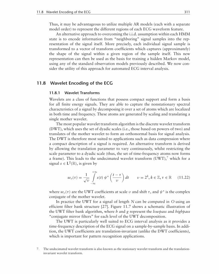
In practice the UWT for a signal of length N can be computed in O using anefficient filter bank structure [27]. Figure 11.7 shows a schematic illustration ofthe UWT filter bank algorithm, where h and g represent the lowpass and highpass“conjugate mirror filters” for each level of the UWT decomposition.

The UWT is particularly well suited to ECG interval analysis as it provides atime-frequency description of the ECG signal on a sample-by-sample basis. In addi-tion, the UWT coefficients are translation-invariant (unlike the DWT coefficients),which is important for pattern recognition applications.

7. The undecimated wavelet transform is also known as the stationary wavelet transform and the translation-invariant wavelet transform.

P1: Shashi



Figure 11.7 Filter bank for the undecimated wavelet transform. At each level k of the transform, theoperators g and h correspond to the highpass and lowpass conjugate mirror filters at that particularlevel.

11.8.2 HMMs with Wavelet-Encoded ECG

In our experiments we found that the Coiflet wavelet with two vanishing mo-ments resulted in the best overall segmentation performance. Figure 11.8 showsthe squared magnitude responses for the lowpass, bandpass, and highpass filtersassociated with this wavelet (which is commonly known as the coifl wavelet).

In order to use the UWT for ECG encoding, the UWT wavelet coefficients fromlevels 1 to 7 were used to form a seven-dimensional encoding for each ECG signal.Table 11.2 shows the five-fold cross-validation results for HMMs trained on ECGwaveforms from leads II and V2 which had been encoded in this manner (usingrange normalization prior to the encoding).

The results presented in Table 11.2 clearly demonstrate the considerable per-formance improvement of HMMs trained with the UWT encoding (albeit at theexpense of a relatively low percentage of single-beat segmentations), comparedwith similar models trained using the raw ECG time series. In particular, the QandToff single-beat segmentation errors of 5.5 ms and 12.4 ms for lead II, and 3.3 msand 9.5 ms for lead V2, are significantly better than the corresponding errors forthe HMM with an autoregressive observation model.

Despite the performance improvement gained from the use of wavelet methodswith hidden Markov models, the models still suffer from the problem of double-beat segmentations. In the following section we consider a modification to theHMM architecture in order to overcome this problem. In particular, we make useof the knowledge that the double-beat segmentations are characterized by the modelinferring a number of states with a duration that is much shorter than the minimumstate duration observed with real ECG signals. This observation leads on to thesubject of duration constraints for hidden Markov models.

11.9 Duration Modeling for Robust Segmentations

A significant limitation of the standard HMM is the manner in which it models statedurations. For a given state i with self-transition coefficient aii , the probability mass

P1: Shashi


11.9 Duration Modeling for Robust Segmentations 313

Figure 11.8 Squared magnitude responses of the highpass, bandpass, and lowpass filters associ-ated with the coifl wavelet (and associated scaling function) over a range of different levels of theundecimated wavelet transform.

P1: Shashi



Table 11.2 Five-Fold Cross-Validation Results for HMMs Trained on the Wavelet-Encoded ECG Signal Data from Leads II and V2

Lead II


Standard HMMGaussian observation model 29.2% 26.1 3.7 5.0 26.8UWT encoding

Standard HMMGMM observation model 26.4% 12.9 5.5 9.6 12.4UWT encoding

Lead V2


Standard HMMGaussian obsevation model 73.0% 20.0 4.1 8.7 15.8UWT encoding

Standard HMMGMM observation model 59.0% 9.9 3.3 5.9 9.5UWT encoding

The encodings are derived from the seven-dimensional coifl wavelet coefficients resulting from alevel 7 UWT decomposition of each ECG signal. In each case range normalization was used priorto the encoding.

function for the state duration d is a geometric distribution, given by

pi (d) = (aii )d−1(1 − aii ) (11.23)

For the waveform features of the ECG signal, this geometric distribution isinappropriate. In particular, the distribution naturally favors state sequences of avery short duration. Conversely, real-world ECG waveform features do not occurfor arbitrarily short durations, and there is typically a minimum duration for each ofthe ECG features. In practice this “mismatch” between the statistical properties ofthe model and those of the ECG results in unreliable “double-beat” segmentations,as discussed previously in Section 11.7.3.

Unfortunately, double-beat segmentations can significantly impact upon the re-liability of the automated QT interval measurements produced by the model. Thus,in order to make use of the model for automated QT interval analysis, the ro-bustness of the segmentation process must be improved. This can be achieved byincorporating duration constraints into the HMM architecture. Each duration con-straint takes the form of a number specifying the minimum duration for a particularstate in the model. For example, the duration constraint for the T wave state is sim-ply the minimum possible duration (in samples) for a T wave. Such values can beestimated in practice by examining the durations of the waveform features for alarge number of annotated ECG waveforms.

Once the duration constraints have been chosen, they are incorporated intothe model in the following manner: For each state k with a minimum duration ofdmin(k), we augment the model with dmin(k) − 1 additional states directly preceding

P1: Shashi


11.9 Duration Modeling for Robust Segmentations 315

Figure 11.9 Graphical illustration of incorporating a duration constraint into an HMM (the dashedbox indicates tied observation distributions).

Table 11.3 Five-Fold Cross-Validation Results for HMMs with Built-In DurationConstraints Trained on the Wavelet Encoded ECG Signal Data from Leads II and V2

Lead II


Duration-constrained HMMGMM observation model 100.0% 8.3 3.5 7.2 12.7UWT encoding

Lead V2


Duration-constrained HMMGMM observation model 100.0% 9.7 3.9 5.5 11.4UWT encoding

the original state k. Each additional state has a self-transition probability of zero,and a probability of one of transitioning to the state to its right. Thus, taken together,these states form a simple left-right Markov chain, where each state in the chain isonly occupied for at most one time sample (during any run through the chain).

The most important feature of this chain is that the parameters of the obser-vation density for each state are identical to the corresponding parameters of theoriginal state k (this is known as “tying”). Thus the observations associated with thedmin states identified with a particular waveform feature are governed by a single setof parameters (which is shared by all dmin states). The overall procedure for incor-porating duration constraints into the HMM architecture is illustrated graphicallyin Figure 11.9.

Table 11.3 shows the five-fold cross-validation results for a hidden Markovmodel with built-in duration constraints. For each fold of the cross-validationprocedure, the minimum state duration dmin(k) was calculated as 80% of theminimum duration present in the annotated training data for each particular state.The set of duration constraints were then incorporated into the HMM architectureand the resulting model was trained in a supervised fashion.

P1: Shashi



The results demonstrate that the duration constrained HMM eliminates theproblem of double-beat segmentations. In addition, the annotation errors for leadsII are of a comparable standard to the best results presented for the single-beatsegmentations only in the previous section.

11.10 Conclusions

In this chapter we have focused on the two core issues in utilizing a probabilisticmodeling approach for the task of automated ECG interval analysis: the choice ofrepresentation for the ECG signal and the choice of model for the segmentation.We have demonstrated that wavelet methods, and in particular the undecimatedwavelet transform, can be used to generate an encoding of the ECG which is tunedto the unique spectral characteristics of the ECG waveform features. With thisrepresentation the performance of the models on new unseen ECG waveforms issignificantly better than similar models trained on the raw time series data. We havealso shown that the robustness of the segmentation process can be improved throughthe use of state duration constraints with hidden Markov models. With these modelsthe robustness of the resulting segmentations is considerably improved.

A key advantage of probabilistic modeling over traditional techniques for ECGsegmentation is the ability of the model to generate a statistical confidence measurein its analysis of a given ECG waveform. As discussed previously in Section 11.3,current automated ECG interval analysis systems are unable to differentiate be-tween normal ECG waveforms (for which the automated annotations are generallyreliable) and abnormal or unusual ECG waveforms (for which the automated an-notations are frequently unreliable). By utilizing a confidence-based approach toautomated ECG interval analysis, however, we can automatically highlight thosewaveforms which are least suitable to analysis by machine (and thus most in needof analysis by a human expert). This strategy therefore provides an effective way tocombine the twin advantages of manual and automated ECG interval analysis [3].

References

[1] Morganroth, J., and H. M. Pyper, “The Use of Electrocardiograms in Clinical DrugDevelopment: Part 1,” Clinical Research Focus, Vol. 12, No. 5, 2001, pp. 17–23.

[2] Houghton, A. R., and D. Gray, Making Sense of the ECG, London, U.K.: Arnold, 1997.[3] Hughes, N. P., and L. Tarassenko, “Automated QT Interval Analysis with Confidence

Measures,” Computers in Cardiology, Vol. 31, 2004.[4] Jane, R., et al., “Evaluation of an Automatic Threshold Based Detector of Waveform

Limits in Holter ECG with QT Database,” Computers in Cardiology, IEEE Press, 1997,pp. 295–298.

[5] Pan, J., and W. J. Tompkins, “A Real-Time QRS Detection Algorithm,” IEEE Trans.Biomed. Eng., Vol. 32, No. 3, 1985, pp. 230–236.

[6] Lepeschkin, E., and B. Surawicz, “The Measurement of the Q-T Interval of the Electro-cardiogram,” Circulation, Vol. VI, September 1952, pp. 378–388.

[7] Xue, Q., and S. Reddy, “Algorithms for Computerized QT Analysis,” Journal of Electro-cardiology, Supplement, Vol. 30, 1998, pp. 181–186.

chapter 11 probabilistic approaches to ecg …gari/ecgbook/ch11.pdf · this rhythm can degenerate...

Documents