chapter 1schwicht/lectures/logic/ws19/log.pdf · chapter 1 logic the main subject of mathematical...
TRANSCRIPT

CHAPTER 1
Logic
The main subject of Mathematical Logic is mathematical proof. In thisintroductory chapter we deal with the basics of formalizing such proofs and,via normalization, analysing their structure. The system we pick for therepresentation of proofs is Gentzen’s natural deduction from (1935). Ourreasons for this choice are twofold. First, as the name says this is a naturalnotion of formal proof, which means that the way proofs are representedcorresponds very much to the way a careful mathematician writing out alldetails of an argument would proceed anyway. Second, formal proofs innatural deduction are closely related (via the so-called Curry-Howard cor-respondence) to terms in typed lambda calculus. This provides us not onlywith a compact notation for logical derivations (which otherwise tend to be-come somewhat unmanagable tree-like structures), but also opens up a routeto applying the computational techniques which underpin lambda calculus.
An underlying theme of this chapter is to bring out the constructivecontent of logic, particularly in regard to the relationship between minimaland classical logic. For us the latter is most appropriately viewed as asubsystem of the former. This approach will reveal some interesting aspectsof proofs, e.g., that it is possible and useful to distinguish beween existentialproofs that actually construct witnessing objects, and others that don’t.
As an example for a non-constructive existence proof, consider the fol-lowing proposition.
There are irrational numbers a, b such that ab is rational.
This can be proved as follows, by cases.
Case√
2√2
is rational. Choose a =√
2 and b =√
2. Then a, b areirrational and by assumption ab is rational.
Case√
2√2
is irrational. Choose a =√
2√2
and b =√
2. Then byassumption a, b are irrational and
ab =(√
2
√2)√2
=(√
2)2
= 2
is rational.
3

4 1. LOGIC
As long as we have not decided whether√
2√2
is rational, we do notknow which numbers a, b we must take. Hence we have an example of anexistence proof which does not provide an instance.
Weyl (1921) gave a somewhat drastic description of this situation:
Ein Existentialsatz – etwa “es gibt eine gerade Zahl” –ist uberhaupt kein Urteil im eigentlichen Sinne, das einenSachverhalt behauptet; Existentialsachverhalte sind eineleere Erfindung der Logiker. “2 ist eine gerade Zahl”, dasist ein wirkliches, einem Sachverhalt Ausdruck gebendesUrteil; “es gibt eine gerade Zahl” ist nur ein aus diesemUrteil gewonnenes Urteilsabstrakt. Bezeichne ich Erkennt-nis als einen wertvollen Schatz, so ist das Urteilsabstraktein Papier, welches das Vorhandensein eines Schatzes an-zeigt, ohne jedoch zu verraten, an welchem Ort. Seineinziger Wert kann darin liegen, daß es mich antreibt, nachdem Schatze zu suchen.
1.1. Natural deduction
The rules of natural deduction come in pairs: we have an introduc-tion and an elimination rule for each of the logical connectives. The re-sulting system is called minimal logic; it was introduced by Kolmogorov(1932), Gentzen (1935) and Johansson (1937). Notice that no negationis yet present. If we go on and require ex-falso-quodlibet for the nullarypropositional symbol ⊥ (“falsum”) we can embed intuitionistic logic withnegation as A → ⊥. To embed classical logic, we need to go further andadd as an axiom schema the principle of indirect proof, also called stabil-ity (∀~x(¬¬R~x→ R~x ) for relation symbols R), but then it is appropriate torestrict to the language based on→, ∀, ⊥ and ∧. The reason for this restric-tion is that we can neither prove ¬¬∃xA→ ∃xA nor ¬¬(A∨B)→ A∨B, forthere are countermodels to both (the former is Markov’s scheme). However,we can prove them for the classical existential quantifier and disjunctiondefined by ¬∀x¬A and ¬A → ¬B → ⊥. Thus we need to make a distinc-tion between two kinds of “exists” and two kinds of “or”: the classical onesare “weak” and the non-classical ones “strong” since they have constructivecontent. In situations where both kinds occur together we must mark thedistinction, and we shall do this by writing a tilde above the weak disjunctionand existence symbols thus ∨, ∃.
1.1.1. Terms and formulas. Let a countably infinite set { vi | i ∈ N }of variables be given; they will be denoted by x, y, z. A first-order languageL then is determined by its signature, which is to mean the following.
1.1. NATURAL DEDUCTION 5
(i) For every natural number n ≥ 0 a (possible empty) set of n-ary rela-tion symbols (or predicate symbols). 0-ary relation symbols are calledpropositional symbols. ⊥ (read “falsum”) is required as a fixed proposi-tional symbol. The language will not, unless stated otherwise, contain= as a primitive. Binary relation symbols can be marked as infix.
(ii) For every natural number n ≥ 0 a (possible empty) set of n-ary functionsymbols. 0-ary function symbols are called constants. Binary functionsymbols can again be marked as infix.
We assume that all these sets of variables, relation and function symbols aredisjoint. L is kept fixed and will only be mentioned when necessary.
Terms are inductively defined as follows.
(i) Every variable is a term.(ii) Every constant is a term.(iii) If t1, . . . , tn are terms and f is an n-ary function symbol with n ≥ 1,
then f(t1, . . . , tn) is a term. (If t, s are terms and ◦ is a binary functionsymbol, then (t ◦ s) is a term.)
From terms one constructs prime formulas, also called atomic formulasor just atoms: If t1, . . . , tn are terms and R is an n-ary relation symbol, thenR(t1, . . . , tn) is a prime formula. (If t, s are terms and ∼ is a binary relationsymbol, then (t ∼ s) is a prime formula.)
Formulas are inductively defined from prime formulas by
(i) Every prime formula is a formula.(ii) If A and B are formulas, then so are (A→ B) (“if A then B”), (A∧B)
(“A and B”) and (A ∨B) (“A or B”).(iii) If A is a formula and x is a variable, then ∀xA (“A holds for all x”)
and ∃xA (“there is an x such that A”) are formulas.
Negation is defined by¬A := (A→ ⊥).
We shall often need to do induction on the height, denoted |A|, offormulas A. This is defined as follows: |P | = 0 for atoms P , |A ◦ B| =max(|A|, |B|) + 1 for binary operators ◦ (i.e., →,∧,∨) and | ◦ A| = |A| + 1for unary operators ◦ (i.e., ∀x, ∃x).
1.1.2. Substitution, free and bound variables. Expressions E , E ′which differ only in the names of bound (occurrences of) variables will beregarded as identical. This is sometimes expressed by saying that E and E ′are α-equal. In other words, we are only interested in expressions “modulorenaming of bound variables”. There are methods of finding unique repre-sentatives for such expressions, e.g., the name-free terms of de Bruijn (1972).For the human reader such representations are less convenient, so we shallstick to the use of bound variables.
6 1. LOGIC
In the definition of “substitution of expression E ′ for variable x in ex-pression E”, either one requires that no variable free in E ′ becomes boundby a variable-binding operator in E , when the free occurrences of x are re-placed by E ′ (also expressed by saying that there must be no “clashes ofvariables”), “E ′ is free for x in E”, or the substitution operation is taken toinvolve a systematic renaming operation for the bound variables, avoidingclashes. Having stated that we are only interested in expressions modulorenaming bound variables, we can without loss of generality assume thatsubstitution is always possible.
Also, it is never a real restriction to assume that distinct quantifieroccurrences are followed by distinct variables, and that the sets of boundand free variables of a formula are disjoint.
Notation. “FV” is used for the (set of) free variables of an expression;so FV(t) is the set of variables free in the term t, FV(A) the set of variablesfree in formula A etc. A formula A is said to be closed if FV(A) = ∅.E [x := t] denotes the result of substituting the term t for the variable
x in the expression E . Similarly, E [~x := ~t ] is the result of simultaneouslysubstituting the terms ~t = t1, . . . , tn for the variables ~x = x1, . . . , xn, respec-tively.
In a given context we shall adopt the following convention. Once aformula has been introduced as A(x), i.e., A with a designated variable x,we write A(t) for A[x := t], and similarly with more variables.
1.1.3. Subformulas. Unless stated otherwise, the notion of subfor-mula will be that defined by Gentzen.
Definition. (Gentzen) subformulas of A are defined by
(a) A is a subformula of A;(b) if B ◦ C is a subformula of A then so are B, C, for ◦ = →,∧,∨;(c) if ∀xB(x) or ∃xB(x) is a subformula of A, then so is B(t).
Definition. The notions of positive, negative, strictly positive subfor-mula are defined in a similar style:
(a) A is a positive and a strictly positive subformula of itself;(b) if B ∧ C or B ∨ C is a positive (negative, strictly positive) subformula
of A, then so are B, C;(c) if ∀xB(x) or ∃xB(x) is a positive (negative, strictly positive) subformula
of A, then so is B(t);(d) if B → C is a positive (negative) subformula of A, then B is a negative
(positive) subformula of A, and C is a positive (negative) subformula ofA;
(e) if B → C is a strictly positive subformula of A, then so is C.

1.1. NATURAL DEDUCTION 7
A strictly positive subformula of A is also called a strictly positive part(s.p.p.) of A. Note that the set of subformulas of A is the union of thepositive and negative subformulas of A.
Example. (P → Q) → R ∧ ∀xS(x) has as s.p.p.’s the whole formula,R ∧ ∀xS(x), R, ∀xS(x), S(t). The positive subformulas are the s.p.p.’s andin addition P ; the negative subformulas are P → Q, Q.
1.1.4. Examples of derivations. To motivate the rules for naturaldeduction, let us start with informal proofs of some simple logical facts.
(A→ B → C)→ (A→ B)→ A→ C.
Informal proof. Assume A → B → C. To show: (A → B) → A → C.So assume A → B. To show: A → C. So finally assume A. To show: C.Using the third assumption twice we have B → C by the first assumption,and B by the second assumption. From B → C and B we then obtainC. Then A → C, cancelling the assumption on A; (A → B) → A → Ccancelling the second assumption; and the result follows by cancelling thefirst assumption. �
∀x(A→ B)→ A→ ∀xB, if x /∈ FV(A).
Informal proof. Assume ∀x(A→ B). To show: A→ ∀xB. So assume A. Toshow: ∀xB. Let x be arbitrary; note that we have not made any assumptionson x. To show: B. We have A → B by the first assumption. Hence alsoB by the second assumption. Hence ∀xB. Hence A → ∀xB, cancelling thesecond assumption. Hence the result, cancelling the first assumption. �
A characteristic feature of these proofs is that assumptions are intro-duced and eliminated again. At any point in time during the proof the freeor “open” assumptions are known, but as the proof progresses, free assump-tions may become cancelled or “closed” because of the implies-introductionrule.
We reserve the word proof for the informal level; a formal representationof a proof will be called a derivation.
An intuitive way to communicate derivations is to view them as labelledtrees each node of which denotes a rule application. The labels of the innernodes are the formulas derived as conclusions at those points, and the labelsof the leaves are formulas or terms. The labels of the nodes immediatelyabove a node k are the premises of the rule application. At the root ofthe tree we have the conclusion (or end formula) of the whole derivation.In natural deduction systems one works with assumptions at leaves of thetree; they can be either open or closed (cancelled). Any of these assump-tions carries a marker . As markers we use assumption variables denotedu, v, w, u0, u1, . . . . The variables of the language previously introduced will

8 1. LOGIC
now often be called object variables, to distinguish them from assumptionvariables. If at a node below an assumption the dependency on this as-sumption is removed (it becomes closed) we record this by writing down theassumption variable. Since the same assumption may be used more thanonce (this was the case in the first example above), the assumption markedwith u (written u : A) may appear many times. Of course we insist thatdistinct assumption formulas must have distinct markers. An inner node ofthe tree is understood as the result of passing from premises to the conclu-sion of a given rule. The label of the node then contains, in addition to theconclusion, also the name of the rule. In some cases the rule binds or closesor cancels an assumption variable u (and hence removes the dependency ofall assumptions u : A thus marked). An application of the ∀-introductionrule similarly binds an object variable x (and hence removes the dependencyon x). In both cases the bound assumption or object variable is added tothe label of the node.
Definition. A formula A is called derivable (in minimal logic), writ-ten ` A, if there is a derivation of A (without free assumptions) usingthe natural deduction rules. A formula B is called derivable from assump-tions A1, . . . , An, if there is a derivation of B with free assumptions amongA1, . . . , An. Let Γ be a (finite or infinite) set of formulas. We write Γ ` B ifthe formula B is derivable from finitely many assumptions A1, . . . , An ∈ Γ.
We now formulate the rules of natural deduction.
1.1.5. Introduction and elimination rules for → and ∀. First wehave an assumption rule, allowing to write down an arbitrary formula Atogether with a marker u:
u : A assumption.
The other rules of natural deduction split into introduction rules (I-rules forshort) and elimination rules (E-rules) for the logical connectives which, forthe time being, are just→ and ∀. For implication→ there is an introductionrule →+ and an elimination rule →− also called modus ponens. The leftpremise A→ B in →− is called the major (or main) premise, and the rightpremise A the minor (or side) premise. Note that with an application of the→+-rule all assumptions above it marked with u : A are cancelled (whichis denoted by putting square brackets around these assumptions), and theu then gets written alongside. There may of course be other uncancelledassumptions v : A of the same formula A, which may get cancelled at a later

1.1. NATURAL DEDUCTION 9
stage.[u : A]
|MB →+uA→ B
|MA→ B
| NA →−B
For the universal quantifier ∀ there is an introduction rule ∀+ (again marked,but now with the bound variable x) and an elimination rule ∀− whose rightpremise is the term t to be substituted. The rule ∀+x with conclusion ∀xAis subject to the following (eigen-)variable condition: the derivation M ofthe premise A must not contain any open assumption having x as a freevariable.
|MA ∀+x∀xA
|M∀xA(x) t
∀−A(t)
We now give derivations of the two example formulas treated informallyabove. Since in many cases the rule used is determined by the conclusion,we suppress in such cases the name of the rule.
u : A→ B → C w : AB → C
v : A→ B w : AB
C →+wA→ C →+v(A→ B)→ A→ C
→+u(A→ B → C)→ (A→ B)→ A→ C
u : ∀x(A→ B) x
A→ B v : AB ∀+x∀xB →+vA→ ∀xB →+u∀x(A→ B)→ A→ ∀xB
Note that the variable condition is satisfied: x is not free in A (and also notfree in ∀x(A→ B)).
1.1.6. Properties of negation. Recall that negation is defined by¬A := (A→ ⊥). The following can easily be derived.
A→ ¬¬A,¬¬¬A→ ¬A.
However, ¬¬A → A is in general not derivable (without stability – we willcome back to this later on).

10 1. LOGIC
Lemma. The following are derivable.
(A→ B)→ ¬B → ¬A,¬(A→ B)→ ¬B,
¬¬(A→ B)→ ¬¬A→ ¬¬B,(⊥ → B)→ (¬¬A→ ¬¬B)→ ¬¬(A→ B),
¬¬∀xA→ ∀x¬¬A.
Derivations are left as an exercise.
1.1.7. Introduction and elimination rules for disjunction ∨, con-junction ∧ and existence ∃. For disjunction the introduction and elimi-nation rules are
|MA ∨+0
A ∨B
|MB ∨+1
A ∨B
|MA ∨B
[u : A]
| NC
[v : B]
| KC ∨−u, v
C
For conjunction we have
|MA
| NB ∧+A ∧B
|MA ∧B
[u : A] [v : B]
| NC ∧− u, v
C
and for the existential quantifier
t
|MA(t)
∃+∃xA(x)
|M∃xA
[u : A]
| NB ∃−x, u (var.cond.)
B
Similar to ∀+x the rule ∃−x, u is subject to an (eigen-)variable condition:in the derivation N the variable x (i) should not occur free in the formulaof any open assumption other than u : A, and (ii) should not occur free inB.
Again, in each of the elimination rules ∨−, ∧− and ∃− the left premiseis called major (or main) premise, and the right premise is called the minor(or side) premise.
It is easy to see that for each of the connectives ∨, ∧, ∃ the rules and thefollowing axioms are equivalent over minimal logic; this is left as an exercise.

1.1. NATURAL DEDUCTION 11
For disjunction the introduction and elimination axioms are
∨+0 : A→ A ∨B,∨+1 : B → A ∨B,∨− : A ∨B → (A→ C)→ (B → C)→ C.
For conjunction we have
∧+ : A→ B → A ∧B, ∧− : A ∧B → (A→ B → C)→ C
and for the existential quantifier
∃+ : A→ ∃xA, ∃− : ∃xA→ ∀x(A→ B)→ B (x /∈ FV(B)).
Remark. All these axioms can be seen as special cases of a generalschema, that of an inductively defined predicate, which is defined by someintroduction rules and one elimination rule.
We collect some easy facts about derivability; B ← A means A→ B.
Lemma. The following are derivable.
(A ∧B → C)↔ (A→ B → C),
(A→ B ∧ C)↔ (A→ B) ∧ (A→ C),
(A ∨B → C)↔ (A→ C) ∧ (B → C),
(A→ B ∨ C)← (A→ B) ∨ (A→ C),
(∀xA→ B)← ∃x(A→ B) if x /∈ FV(B),
(A→ ∀xB)↔ ∀x(A→ B) if x /∈ FV(A),
(∃xA→ B)↔ ∀x(A→ B) if x /∈ FV(B),
(A→ ∃xB)← ∃x(A→ B) if x /∈ FV(A).
Proof. A derivation of the final formula is
u : ∃x(A→ B)x
w : A→ B v : AB
∃xB ∃−x,w∃xB →+vA→ ∃xB →+u∃x(A→ B)→ A→ ∃xB
The variable condition for ∃− is satisfied since the variable x (i) is not freein the formula A of the open assumption v : A, and (ii) is not free in ∃xB.The rest of the proof is left as an exercise. �

12 1. LOGIC
As already mentioned, we distinguish between two kinds of “exists” andtwo kinds of “or”: the “weak” or classical ones and the “strong” or non-classical ones, with constructive content. In the present context both kindsoccur together and hence we must mark the distinction; we shall do this bywriting a tilde above the weak disjunction and existence symbols thus
A ∨ B := ¬A→ ¬B → ⊥, ∃xA := ¬∀x¬A.These weak variants of disjunction and the existential quantifier are nostronger than the proper ones (in fact, they are weaker):
A ∨B → A ∨ B, ∃xA→ ∃xA.This can be seen easily by putting C := ⊥ in ∨− and B := ⊥ in ∃−.
Remark. Since ∃x∃yA unfolds into a rather awkward formula we extend
the ∃-terminology to lists of variables:
∃x1,...,xnA := ∀x1,...,xn(A→ ⊥)→ ⊥.Moreover let
∃x1,...,xn(A1 ∧ . . . ∧Am) := ∀x1,...,xn(A1 → · · · → Am → ⊥)→ ⊥.This allows to stay in the →,∀ part of the language. Notice that ∧ onlymakes sense in this context, i.e., in connection with ∃.
1.1.8. Intuitionistic and classical derivability. In the definition ofderivability in Section 1.1.4 falsity ⊥ plays no role. We may change this andrequire ex-falso-quodlibet axioms, of the form
∀~x(⊥ → R~x )
with R a relation symbol distinct from ⊥. Let Efq denote the set of all suchaxioms. A formula A is called intuitionistically derivable, written `i A, ifEfq ` A. We write Γ `i B for Γ ∪ Efq ` B.
We may even go further and require stability axioms, of the form
∀~x(¬¬R~x→ R~x )
with R again a relation symbol distinct from ⊥. Let Stab denote the set ofall these axioms. A formula A is called classically derivable, written `c A,if Stab ` A. We write Γ `c B for Γ ∪ Stab ` B.
It is easy to see that intuitionistically (i.e., from Efq) we can derive⊥ → A for an arbitrary formula A, using the introduction rules for theconnectives. A similar generalization of the stability axioms is only possiblefor formulas in the language not involving ∨,∃. However, it is still possibleto use the substitutes ∨ and ∃.
Theorem (Stability, or principle of indirect proof).

1.1. NATURAL DEDUCTION 13
(a) ` (¬¬A→ A)→ (¬¬B → B)→ ¬¬(A ∧B)→ A ∧B.(b) ` (¬¬B → B)→ ¬¬(A→ B)→ A→ B.(c) ` (¬¬A→ A)→ ¬¬∀xA→ A.(d) `c ¬¬A→ A for every formula A without ∨, ∃.
Proof. (a) is left as an exercise.(b) For simplicity, in the derivation to be constructed we leave out ap-
plications of →+ at the end.
u : ¬¬B → B
v : ¬¬(A→ B)
u1 : ¬Bu2 : A→ B w : A
B⊥ →+u2¬(A→ B)
⊥ →+u1¬¬BB
(c)
u : ¬¬A→ A
v : ¬¬∀xA
u1 : ¬Au2 : ∀xA x
A⊥ →+u2¬∀xA
⊥ →+u1¬¬AA
(d) Induction on A. The case R~t with R distinct from ⊥ is given by Stab.In the case ⊥ the desired derivation is
v : (⊥ → ⊥)→ ⊥u : ⊥ →+u⊥ → ⊥
⊥In the cases A ∧B, A→ B and ∀xA use (a), (b) and (c), respectively. �
Using stability we can prove some well-known facts about the interactionof weak disjunction and the weak existential quantifier with implication. Wefirst prove a more refined claim, stating to what extent we need to go beyondminimal logic.
Lemma. The following are derivable.
(∃xA→ B)→ ∀x(A→ B) if x /∈ FV(B),(1)
(¬¬B → B)→ ∀x(A→ B)→ ∃xA→ B if x /∈ FV(B),(2)
(⊥ → B[x:=c])→ (A→ ∃xB)→ ∃x(A→ B) if x /∈ FV(A),(3)
∃x(A→ B)→ A→ ∃xB if x /∈ FV(A).(4)

14 1. LOGIC
The last two items can also be seen as simplifying a weakly existentiallyquantified implication whose premise does not contain the quantified variable.In case the conclusion does not contain the quantified variable we have
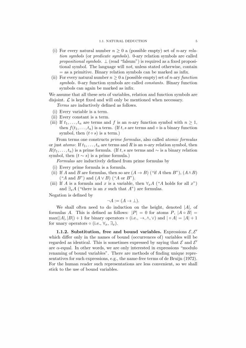
(¬¬B → B)→ ∃x(A→ B)→ ∀xA→ B if x /∈ FV(B),(5)
∀x(¬¬A→ A)→ (∀xA→ B)→ ∃x(A→ B) if x /∈ FV(B).(6)
Proof. (1)
∃xA→ B
u1 : ∀x¬A x¬A A
⊥ →+u1¬∀x¬AB
(2)
¬¬B → B
¬∀x¬A
u2 : ¬B
∀x(A→ B) x
A→ B u1 : AB
⊥ →+u1¬A∀x¬A
⊥ →+u2¬¬BB
(3) Writing B0 for B[x:=c] we have
∀x¬(A→ B) c
¬(A→ B0)
⊥ → B0
A→ ∃xB u2 : A
∃xB
∀x¬(A→ B) x
¬(A→ B)u1 : BA→ B
⊥ →+u1¬B∀x¬B
⊥B0 →+u2
A→ B0
⊥(4)
∃x(A→ B)
∀x¬B x¬B
u1 : A→ B AB
⊥ →+u1¬(A→ B)
∀x¬(A→ B)
⊥
1.1. NATURAL DEDUCTION 15
(5)
¬¬B → B
∃x(A→ B)
u2 : ¬Bu1 : A→ B
∀xA xA
B⊥ →+u1¬(A→ B)
∀x¬(A→ B)
⊥ →+u2¬¬BB
(6) We derive ∀x(⊥ → A) → (∀xA → B) → ∀x¬(A → B) → ¬¬A. WritingAx,Ay for A(x), A(y) we have
∀x¬(Ax→ B) x
¬(Ax→ B)
∀xAx→ B
∀y(⊥ → Ay) y
⊥ → Ayu1 : ¬Ax u2 : Ax
⊥Ay
∀yAyB →+u2
Ax→ B
⊥ →+u1¬¬AxUsing this derivation M we obtain
∀x¬(Ax→ B) x
¬(Ax→ B)
∀xAx→ B
∀x(¬¬Ax→ Ax) x
¬¬Ax→ Ax
|M¬¬Ax
Ax∀xAx
BAx→ B
⊥Since clearly ` (¬¬A→ A)→ ⊥→ A the claim follows. �
Remark. An immediate consequence of (6) is the classical derivability
of the “drinker formula” ∃x(Px → ∀xPx), to be read “in every non-emptybar there is a person such that, if this person drinks, then everybody drinks”.To see this let A := Px and B := ∀xPx in (6).
Corollary.
`c (∃xA→ B)↔ ∀x(A→ B) if x /∈ FV(B) and B without ∨, ∃,
`i (A→ ∃xB)↔ ∃x(A→ B) if x /∈ FV(A),
`c ∃x(A→ B)↔ (∀xA→ B) if x /∈ FV(B) and A,B without ∨,∃.

16 1. LOGIC
There is a similar lemma on weak disjunction:
Lemma. The following are derivable.
(A ∨ B → C)→ (A→ C) ∧ (B → C),(7)
(¬¬C → C)→ (A→ C)→ (B → C)→ A ∨ B → C,(8)
(⊥ → B)→ (A→ B ∨ C)→ (A→ B) ∨ (A→ C),(9)
(A→ B) ∨ (A→ C)→ A→ B ∨ C,(10)
(¬¬C → C)→ (A→ C) ∨ (B → C)→ A→ B → C,(11)
(⊥ → C)→ (A→ B → C)→ (A→ C) ∨ (B → C).(12)
Proof. We only consider (8) and (12); the rest is left as an exercise.(8)
¬¬C → C
¬A→ ¬B → ⊥
u1 : ¬CA→ C u2 : A
C⊥ →+u2¬A
¬B → ⊥
u1 : ¬CB → C u3 : B
C⊥ →+u3¬B
⊥ →+u1¬¬CC
(12)
¬(B → C)
⊥ → C
¬(A→ C)
A→ B → C u1 : AB → C u2 : B
C →+u1A→ C
⊥C →+u2
B → C
⊥The general idea here is to view ∨ as a finitary version of ∃. �
Corollary.
`c (A ∨ B → C)↔ (A→ C) ∧ (B → C) for C without ∨,∃,`i (A→ B ∨ C)↔ (A→ B) ∨ (A→ C),
`c (A→ C) ∨ (B → C)↔ (A→ B → C) for C without ∨, ∃.
The weak existential quantifier ∃ and weak disjunction ∨ satisfy the sameintroduction axioms as the strong ones: this follows from the derivabilityof ∃xA → ∃xA and A ∨ B → A ∨ B (see Section 1.1.7). They also satisfy

1.1. NATURAL DEDUCTION 17
the same elimination axioms, provided one restricts the conclusion to stableformulas. For ∃ this has been proved in (2), and for ∨ in (8).
Therefore when proving a stable goal in minimal logic more proof tech-niques are available than in the general case. For instance, case distinctionon an arbitrary formula A is possible by (8), since A ∨ ¬A is (easily) deriv-able. Another important example is
Lemma. The following is derivable.
∀x¬A ∨ ∃xA.
Proof. Unfolding ∨ and ∃ gives
(∀x(A→ ⊥)→ ⊥)→ ((∀x(A→ ⊥)→ ⊥)︸ ︷︷ ︸∃xA
→ ⊥)→ ⊥. �
It is often helpful to use this lemma in a slightly more general form, forinstancce
∀x,y(A→ B → ⊥) ∨ ∃x,y(A ∧B).
The proof is again immediate, since the right hand side ∃x,y(A ∧B) unfoldsinto the negated left hand side.
1.1.9. Godel-Gentzen translation. Classical derivability Γ `c B wasdefined in Section 1.1.8 by Γ ∪ Stab ` B. This embedding of classical logicinto minimal logic can be expressed in a somewhat different and very explicitform, namely as a syntactic translation A 7→ Ag of formulas such that Ais derivable in classical logic if and only if its translation Ag is derivable inminimal logic.
Definition (Godel-Gentzen translation Ag).
(R~t )g := ¬¬R~t for R distinct from ⊥,⊥g := ⊥,(A ∨B)g := Ag ∨ Bg,
(∃xA)g := ∃xAg,(A ◦B)g := Ag ◦Bg for ◦ = →,∧,(∀xA)g := ∀xAg.
Lemma (Stability of Ag). ` ¬¬Ag → Ag.
Proof. Induction on A.Case R~t with R distinct from ⊥. We must show ¬¬¬¬R~t → ¬¬R~t,
which is a special case of ` ¬¬¬B → ¬B.Case ⊥. Use ` ¬¬⊥ → ⊥.

18 1. LOGIC
Case A ∨ B. We must show ` ¬¬(Ag ∨ Bg) → Ag ∨ Bg, which is aspecial case of ` ¬¬(¬C → ¬D → ⊥)→ ¬C → ¬D → ⊥:
¬¬(¬C → ¬D → ⊥)
u1 : ¬C → ¬D → ⊥ ¬C¬D → ⊥ ¬D
⊥ →+u1¬(¬C → ¬D → ⊥)
⊥Case ∃xA. In this case we must show ` ¬¬∃xAg → ∃xAg, but this is a
special case of ` ¬¬¬B → ¬B, because ∃xAg is the negation ¬∀x¬Ag.Case A ∧ B. We must show ` ¬¬(Ag ∧ Bg) → Ag ∧ Bg. By induction
hypothesis ` ¬¬Ag → Ag and ` ¬¬Bg → Bg. Now use part (a) of thestability theorem in Section 1.1.8.
The cases A → B and ∀xA are similar, using parts (b) and (c) of thestability theorem instead. �
Theorem. (a) Γ `c A implies Γg ` Ag.(b) Γg ` Ag implies Γ `c A for Γ, A without ∨,∃.
Proof. (a) We use induction on Γ `c A. In case of a stability axiom∀~x(¬¬R~x → R~x ) we must derive ∀~x(¬¬¬¬R~x → ¬¬R~x ), which is easy(as above). For the rules →+, →−, ∀+, ∀−, ∧+ and ∧− the claim followsimmediately from the induction hypothesis, using the same rule again. Thisworks because the Godel-Gentzen translation acts as a homomorphism forthese connectives. For the rules ∨+i , ∨−, ∃+ and ∃− the claim follows from
the induction hypothesis and the remark on the elimination rules for ∨, ∃ inSection 1.1.8. For example, in case ∃− the induction hypothesis gives
|M∃xAg
andu : Ag
| NBg
with x /∈ FV(Bg). Now use ` (¬¬Bg → Bg) → ∃xAg → ∀x(Ag → Bg) →Bg. Its premise ¬¬Bg → Bg is derivable by the lemma above.
(b) First note that `c (B ↔ Bg) if B is without ∨,∃. Now assume thatΓ, A are without ∨,∃. From Γg ` Ag we obtain Γ `c A as follows. We argueinformally. Assume Γ. Then Γg by the note, hence Ag because of Γg ` Ag,hence A again by the note. �
1.2. Normalization
A derivation in normal form does not make “detours”, or more precisely,it cannot occur that an elimination rule immediately follows an introductionrule. We use “conversions” to remove such “local maxima” of complexity,thus reducing any given derivation to normal form.

1.2. NORMALIZATION 19
We consider derivations involving →, ∀-rules only, and prove that (i)every such reduction sequence terminates after finitely many steps, and (ii)that the resulting “normal form” is uniquely determined. Uniqueness ofnormal form will be shown by means of an application of Newman’s lemma;we will also introduce and discuss the related notions of confluence, weakconfluence and the Church-Rosser property. Moreover we analyse the shapeof derivations in normal form, and prove the subformula property, which saysthat every formula in a normal derivation is a subformula of the end-formulaor else of an assumption.
We then show that the requirement to give a normal derivation of aderivable formula can sometimes be unrealistic. Following Statman (1978)and Orevkov (1979) we give examples of simple→, ∀-formulas Ci which needderivation height superexponential in i if normal derivations are required,but have non-normal derivations of height linear in i. The non-normalderivations of Ci make use of auxiliary formulas with an i-fold nesting ofimplications and universal quantifiers. This sheds some light on the powerof abstract notions in mathematics: their use can shorten proofs dramati-cally.
1.2.1. The Curry-Howard correspondence. Since natural deduc-tion derivations can be notationally cumbersome, it will be convenient torepresent them as typed “derivation terms”, where the derived formula isthe “type” of the term (and displayed as a superscript). This representa-tion goes under the name of Curry-Howard correspondence. It dates backto Curry (1930) and somewhat later Howard, published only in (1980), whonoted that the types of the combinators used in combinatory logic are ex-actly the Hilbert style axioms for minimal propositional logic. SubsequentlyMartin-Lof (1972) transferred these ideas to a natural deduction settingwhere natural deduction proofs of formulas A now correspond exactly tolambda terms with type A. This representation of natural deduction proofswill henceforth be used consistently.
We give an inductive definition of such derivation terms for the →,∀-rules in Table 1 where for clarity we have written the corresponding deriva-tions to the left. This can be extended to the rules for ∨, ∧ and ∃, but wewill not do this here.
Every derivation term carries a formula as its type. However, we shallusually leave these formulas implicit and write derivation terms withoutthem. Notice that every derivation term can be written uniquely in one ofthe forms
u ~M | λvM | (λvM)N~L,
where u is an assumption variable or assumption constant, v is an assump-tion variable or object variable, and M , N , L are derivation terms or object

20 1. LOGIC
Derivation Term
u : A uA
[u : A]
|MB →+uA→ B
(λuAMB)A→B
|MA→ B
| NA →−B
(MA→BNA)B
|MA ∀+x (with var.cond.)∀xA
(λxMA)∀xA (with var.cond.)
|M∀xA(x) t
∀−A(t)
(M∀xA(x)t)A(t)
Table 1. Derivation terms for → and ∀
terms. Here the final form is not normal: (λvM)N~L is called a β-redex (for“reducible expression”). It can be reduced by a “conversion”. A conversionremoves a detour in a derivation, i.e., an elimination immediately follow-ing an introduction. We consider the following conversions, for derivationswritten in tree notation and also as derivation terms.→-conversion.
[u : A]
|MB →+uA→ B
| NA →−B
7→β
| NA|MB

1.2. NORMALIZATION 21
or written as derivation terms
(λuM(uA)B)A→BNA 7→β M(NA)B.
The reader familiar with λ-calculus should note that this is nothing otherthan β-conversion.∀-conversion.
|MA(x)
∀+x∀xA(x) t∀−
A(t)
7→β|M ′
A(t)
or written as derivation terms
(λxM(x)A(x))∀xA(x)t 7→β M(t).
The closure of the conversion relation 7→β is defined by
(a) If M 7→β M′, then M →M ′.
(b) If M → M ′, then also MN → M ′N , NM → NM ′, λvM → λvM′
(inner reductions).
Therefore M → N means that M reduces in one step to N , i.e., N isobtained from M by replacement of (an occurrence of) a redex M ′ of M bya conversum M ′′ of M ′, i.e., by a single conversion.
Example. Consider assumption variables
x : A→ (B → A)→ A u : A u′ : A
y : A→ B → A v : B → A v′ : B
z : A
Then we have derivation terms
S := λxλyλz(xz(yz))A : (A→ (B → A)→ A)→ (A→ B → A)→ A→ A
K := λuλvu : A→ (B → A)→ A
K ′ := λu′λv′u′ : A→ B → A
By the one step reduction relation we obtain
SKK ′ → (λxλyλz(xz(yz)))(λuλv u)(λu′λv′ u′)→
(λyλz((λuλv u)z(yz)))(λu′λv′ u′) →
(λyλz((λv z)(yz)))(λu′λv′ u′) →
(λyλz z)(λu′λv′ u′) → λz z.
The relation →+ (“properly reduces to”) is the transitive closure of →,and →∗ (“reduces to”) is the reflexive and transitive closure of →. Therelation →∗ is said to be the notion of reduction generated by 7→.

22 1. LOGIC
Lemma (Substitutivity of →).
(a) If M(v)→M ′(v), then M(N)→M ′(N).(b) If N → N ′, then M(N)→∗ M(N ′).
Proof. (a) is proved by induction on M(v)→M ′(v); (b) by inductionon M(v). Notice that the reason for →∗ in (b) is the fact that v may havemany occurrences in M(v). �
1.2.2. Strong normalization. A term M is in normal form, or M isnormal , if M does not contain a redex. M has a normal form if there is anormal N such that M →∗ N . A reduction sequence is a (finite or infinite)sequence M0 → M1 → M2 . . . such that Mi → Mi+1, for all i. Finitereduction sequences are partially ordered under the initial part relation; thecollection of finite reduction sequences starting from a term M forms a tree,the reduction tree of M . The branches of this tree may be identified withthe collection of all infinite and all terminating finite reduction sequences.A term is strongly normalizing if its reduction tree is finite.
We show that every term is strongly normalizing. To this end, define byrecursion on k a relation sn(M,k) between terms M and natural numbersk with the intention that k is an upper bound on the number of reductionsteps up to normal form.
sn(M, 0) := M is in normal form,
sn(M,k + 1) := sn(M ′, k) for all M ′ such that M →M ′.
Clearly a term is strongly normalizing if there is a k such that sn(M,k).We first prove some closure properties of the relation sn, but a word about
notation is crucial here. Whenever we write an applicative term as M ~N :=MN1 . . . Nk the convention is that bracketing to the left operates. That is,
M ~N = (. . . (MN1) . . . Nk).
Lemma (Properties of sn). (a) If sn(M,k), then sn(M,k + 1).(b) If sn(MN, k), then sn(M,k).(c) If sn(Mi, ki) for i = 1 . . . n, then sn(uM1 . . .Mn, k1 + · · ·+ kn).(d) If sn(M,k), then sn(λvM,k).
(e) If sn(M(N)~L, k) and sn(N, l), then sn((λvM(v))N~L, k + l + 1).
Proof. (a) Induction on k. Assume sn(M,k). We show sn(M,k + 1).Let M ′ with M → M ′ be given; because of sn(M,k) we must have k > 0.We have to show sn(M ′, k). Because of sn(M,k) we have sn(M ′, k − 1),hence by induction hypothesis sn(M ′, k).
(b) Induction on k. Assume sn(MN, k). We show sn(M,k). In case k =0 the term MN is normal, hence also M is normal and therefore sn(M, 0).Let k > 0 and M → M ′; we have to show sn(M ′, k − 1). From M →
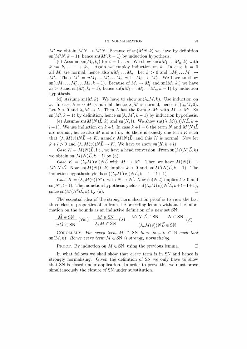
1.2. NORMALIZATION 23
M ′ we obtain MN → M ′N . Because of sn(MN, k) we have by definitionsn(M ′N, k − 1), hence sn(M ′, k − 1) by induction hypothesis.
(c) Assume sn(Mi, ki) for i = 1 . . . n. We show sn(uM1 . . .Mn, k) withk := k1 + · · · + kn. Again we employ induction on k. In case k = 0all Mi are normal, hence also uM1 . . .Mn. Let k > 0 and uM1 . . .Mn →M ′. Then M ′ = uM1 . . .M
′i . . .Mn with Mi → M ′i . We have to show
sn(uM1 . . .M′i . . .Mn, k − 1). Because of Mi → M ′i and sn(Mi, ki) we have
ki > 0 and sn(M ′i , ki − 1), hence sn(uM1 . . .M′i . . .Mn, k − 1) by induction
hypothesis.(d) Assume sn(M,k). We have to show sn(λvM,k). Use induction on
k. In case k = 0 M is normal, hence λvM is normal, hence sn(λvM, 0).Let k > 0 and λvM → L. Then L has the form λvM
′ with M → M ′. Sosn(M ′, k − 1) by definition, hence sn(λvM
′, k − 1) by induction hypothesis.
(e) Assume sn(M(N)~L, k) and sn(N, l). We show sn((λvM(v))N~L, k +
l+ 1). We use induction on k+ l. In case k+ l = 0 the term N and M(N)~Lare normal, hence also M and all Li. So there is exactly one term K such
that (λvM(v))N~L → K, namely M(N)~L, and this K is normal. Now let
k + l > 0 and (λvM(v))N~L→ K. We have to show sn(K, k + l).
Case K = M(N)~L, i.e., we have a head conversion. From sn(M(N)~L, k)
we obtain sn(M(N)~L, k + l) by (a).
Case K = (λvM′(v))N~L with M → M ′. Then we have M(N)~L →
M ′(N)~L. Now sn(M(N)~L, k) implies k > 0 and sn(M ′(N)~L, k − 1). The
induction hypothesis yields sn((λvM′(v))N~L, k − 1 + l + 1).
Case K = (λvM(v))N ′~L with N → N ′. Now sn(N, l) implies l > 0 and
sn(N ′, l−1). The induction hypothesis yields sn((λvM(v))N ′~L, k+l−1+1),
since sn(M(N ′)~L, k) by (a). �
The essential idea of the strong normalization proof is to view the lastthree closure properties of sn from the preceding lemma without the infor-mation on the bounds as an inductive definition of a new set SN:
~M ∈ SN (Var)u ~M ∈ SN
M ∈ SN (λ)λvM ∈ SN
M(N)~L ∈ SN N ∈ SN(β)
(λvM(v))N~L ∈ SN
Corollary. For every term M ∈ SN there is a k ∈ N such thatsn(M,k). Hence every term M ∈ SN is strongly normalizing.
Proof. By induction on M ∈ SN, using the previous lemma. �
In what follows we shall show that every term is in SN and hence isstrongly normalizing. Given the definition of SN we only have to showthat SN is closed under application. In order to prove this we must provesimultaneously the closure of SN under substitution.

24 1. LOGIC
Theorem (Properties of SN). For all formulas A,
(a) for all M(v) ∈ SN, if NA ∈ SN, then M(N) ∈ SN,(b) for all M(x) ∈ SN, M(t) ∈ SN,(c) if M ∈ SN derives A→ B and NA ∈ SN, then MN ∈ SN,(d) if M ∈ SN derives ∀xA, then Mt ∈ SN.
Proof. By course-of-values induction on |A|, with a side induction onM ∈ SN. Let NA ∈ SN. We distinguish cases on the form of M .
Case u ~M by (Var) from ~M ∈ SN. (a) The side induction hypothesis
(a) yields Mi(N) ∈ SN for all Mi from ~M . In case u 6= v we immediately
have u ~M(N) ∈ SN. Otherwise we need N ~M(N) ∈ SN. But this follows bymultiple applications of induction hypothesis (c), since every Mi(N) derivesa subformula of A with smaller height. (b) Similar, and simpler. (c), (d)Use (Var) again.
Case λvM by (λ) from M ∈ SN. (a), (b) Use (λ) again. (c) Our goal is(λvM(v))N ∈ SN. By (β) it suffices to show M(N) ∈ SN and N ∈ SN. Thelatter holds by assumption, and the former by the side induction hypothesis(a). (d) Similar, and simpler.
Case (λwM(w))K~L by (β) from M(K)~L ∈ SN and K ∈ SN. (a) The
side induction hypothesis (a) yields M(N)(K(N))~L(N) ∈ SN and K(N) ∈SN, hence (λwM(N))K(N)~L(N) ∈ SN by (β). (b) Similar, and simpler.(c), (d) Use (β) again. �
Corollary. For every term we have M ∈ SN; in particular every termM is strongly normalizing.
Proof. Induction on the (first) inductive definition of derivation termsM . In cases u and λvM the claim follows from the definition of SN, and incase MN it follows from the preceding theorem. �
Remark. It may well happen that reasonable “simplification” steps onderivations lead to reduction loops. The following example is due to Ekman(1994). Consider the derivation
u : A→ A→ B
v : (A→ B)→ A
u : A→ A→ B w : AA→ B w : A
B →+wA→ B (∗)
AA→ B (∗)
|MA
B

1.2. NORMALIZATION 25
where M is
v : (A→ B)→ A
u : A→ A→ B w : AA→ B w : A
B →+wA→ B
A
Its derivation term is
u(vλw(uww))(vλw(uww)).
Here the following “pruning” simplification can be performed. In betweenthe two occurrences of A → B marked with (∗) no →+ rule is applied.Therefore we may cut out or prune the intermediate part and obtain
u : A→ A→ B w : AA→ B w : A
B →+wA→ B
|MA
B
whose derivation term is
(λw(uww))(vλw(uww)).
But now an →-conversion can be performed, which leads to the derivationwe started with.
1.2.3. Uniqueness of normal forms. We show that normal formsw.r.t. the →,∀-conversions are uniquely determined. This is also expressedby saying that the reduction relation is “confluent”. The proof relies on thefact that the reduction relation terminates, and uses Newman’s lemma toinfer confluence from the (easy to prove) “local confluence”.
A relation → is said to be confluent , or to have the Church-Rosserproperty (CR), if, whenever M0 → M1 and M0 → M2, then there is an M3
such that M1 → M3 and M2 → M3. A relation → is said to be weaklyconfluent , or to have the weak Church-Rosser property (WCR), if, wheneverM0 → M1 and M0 → M2 then there is an M3 such that M1 →∗ M3 andM2 →∗ M3, where →∗ is the reflexive and transitive closure of →.
Lemma (Newman (1942)). Assume that→ is weakly confluent. Then thenormal form w.r.t.→ of a strongly normalizing M is unique. Moreover, if allterms are strongly normalizing w.r.t. →, then the relation →∗ is confluent.
Proof. We write N ← M for M → N , and N ←∗ M for M →∗ N .Call M good if it satisfies the confluence property w.r.t. →∗, i.e., wheneverK ←∗ M →∗ L, then K →∗ N ←∗ L for some N . We show that everystrongly normalizing M is good, by transfinite induction on the well-founded

26 1. LOGIC
M�
��@@@R
M ′ weak conf.M ′′
���∗ @
@@R∗ �
��∗ @
@@R∗
K IH(M ′) ∃N ′ L@@@R∗ �
��∗ �
���
��
∗IH(M ′′)
∃N ′′@@@R∗
∃N
Figure 1. Proof of Newman’s lemma
partial order →+, restricted to all terms occurring in the reduction tree ofM . So let M be given and assume
every M ′ with M →+ M ′ is good.
We must show that M is good, so assume K ←∗ M →∗ L. We may furtherassume that there are M ′,M ′′ such that K ←∗ M ′ ← M → M ′′ →∗ L, forotherwise the claim is trivial. But then the claim follows from the assumedweak confluence and the induction hypothesis for M ′ and M ′′, as shown inFigure 1. �
Proposition. → is weakly confluent.
Proof. Assume N0 ← M → N1. We show that N0 →∗ N ←∗ N1 forsome N , by induction on M . If there are two inner reductions both on thesame subterm, then the claim follows from the induction hypothesis usingsubstitutivity. If they are on distinct subterms, then the subterms do notoverlap and the claim is obvious. It remains to deal with the case of a headreduction together with an inner conversion. This is done in Figure 2, wherefor the lower left arrows we have used substitutivity again. �
Corollary. Normal forms are unique.
Proof. By the proposition → is weakly confluent. From this and thefact that it is strongly normalizing we can infer (using Newman’s lemma)that normal forms are unique. �
1.2.4. The structure of normal derivations. To analyze normalderivations, it will be useful to introduce the notion of a track in a prooftree, which makes sense for non-normal derivations as well.

1.2. NORMALIZATION 27
(λvM(v))N~L���
@@@R
M(N)~L@@@R
(λvM′(v))N~L
���
M ′(N)~L
(λvM(v))N~L�
��@@@R
M(N)~L@@@R∗
(λvM(v))N ′~L�
��M(N ′)~L
(λvM(v))N~L�
��@@@R
M(N)~L@@@R
(λvM(v))N~L′
���
M(N)~L′
Figure 2. Weak concluence of →
Definition. A track of a derivation M is a sequence of formula occur-rences (f.o.) A0, . . . , An such that
(a) A0 is a top f.o. in M ;(b) Ai for i < n is not the minor premise of an instance of →−, and Ai+1 is
directly below Ai;(c) An is either the minor premise of an instance of →−, or the conclusion
of M .
The track of order 0, or main track , in a derivation is the (unique) trackending in the conclusion of the whole derivation. A track of order n + 1is a track ending in the minor premise of an →−-application, with majorpremise belonging to a track of order n.
Lemma. In a derivation each formula occurrence belongs to some track.
Proof. By induction on derivations. �
Now consider a normal derivation M . Since by normality an E-rulecannot have the conclusion of an I-rule as its major premise, the E-ruleshave to precede the I-rules in a track, so the following is obvious: a trackmay be divided into an E-part, say A0, . . . , Ai−1, a minimal formula Ai, andan I-part Ai+1, . . . , An. In the E-part all rules are E-rules; in the I-part allrules are I-rules; Ai is the conclusion of an E-rule and, if i < n, a premiseof an I-rule. Tracks are pieces of branches of the tree with successive f.o.’sin the subformula relationship: either Ai+1 is a subformula of Ai or viceversa. As a result, all formulas in a track A0, . . . , An are subformulas of A0

28 1. LOGIC
or of An; and from this, by induction on the order of tracks, we see thatevery formula in M is a subformula either of an open assumption or of theconclusion. To summarize:
Theorem (Subformula property). In a normal derivation each formulais a subformula of either the end formula or else an assumption formula.
Proof. One proves this for tracks of order n, by induction on n. �
Notice that the minimal formula in a track can be an implication A→ Bor generalization ∀xA. However, we can apply an “η-expansion” and replacethe occurrence of A→ B or ∀xA by
A→ B u : A →−B →+uA→ B
∀xA x∀−A ∀+x∀xA
Repeating this process we obtain a derivation in “long normal form”, all ofwhose minimal formulas are neither implications nor generalizations.
1.2.5. Normal vs. non-normal derivations. Based on work of Stat-man (1978) and in partiular Orevkov (1979) we give examples of →,∀-formulas Ci which need derivation height superexponential in i if normalderivations are required, but have non-normal derivations of height linear ini. The proofs are left as exercises.
We work in a language with a ternary relation symbol R, a constant 0and a unary function symbol S. The intuitive meaning of Ryxz is y+2x = z,and we can express this by means of two (“Horn”-) clauses
Hyp1 := ∀yR(y, 0, Sy),
Hyp2 := ∀y,x,z,z1(Ryxz → Rzxz1 → R(y, Sx, z1)).
Let
Di := ∃zi,zi−1,...,z0(R00zi ∧R0zizi−1 ∧ . . . ∧R0z1z0),
Ci := Hyp1 → Hyp2 → Di.
(for ∧ cf. the remark at the end of Section 1.1.7). Di intuitively means thatthere are numbers zi = 1, zi−1 = 2zi = 2, zi−2 = 2zi−1 = 22, zi−3 = 2zi−2 =
222
and finally z0 = 2i (where 20 := 1, 2n+1 := 22n).To obtain short derivations of Ci we use the following “lifting” formulas:
A0(x) := ∀y∃zRyxz,
Ai+1(x) := ∀y∈Ai ∃z∈AiRyxz,
where ∀z∈AiB abbreviates ∀z(Ai(z)→ B).
Lemma. There are derivations of

1.3. SOUNDNESS AND COMPLETENESS FOR TREE MODELS 29
(a) ∀x(Ai(x)→ Ai(Sx)) from Hyp2 and of(b) Ai(0) from Hyp1 and Hyp2,
both of constant height (i.e., height independent of i).
Proof. Exercise. �
Proposition. There are derivations of Di from Hyp1 and Hyp2 withheight linear in i.
Proof. Exercise. �
Theorem. Every normal derivation of Di from Hyp1, Hyp2 has at least2i nodes.
Proof. Exercise. �
1.3. Soundness and completeness for tree models
It is an obvious question to ask whether the logical rules we have beenconsidering suffice, i.e., whether we have forgotten some necessary rules. Toanswer this question we first have to fix the meaning of a formula, i.e., pro-vide a semantics. This will be done by means of the tree models introducedby Beth (1956). Using this concept of a model we will prove soundness andcompleteness.
1.3.1. Tree models. Consider a finitely branching tree of “possibleworlds”. The worlds are represented as nodes in this tree. They may bethought of as possible states such that all nodes “above” a node k are theways in which k may develop in the future. The worlds are increasing; thatis, if an atomic formula R~t is true in a world k, then R~t is true in all futureworlds k′.
More formally, each tree model is based on a finitely branching tree T . Anode k over a set S is a finite sequence k = 〈a0, a1, . . . , an−1〉 of elements ofS; lh(k) is the length of k. We write k � k′ if k is an initial segment of k′. Atree on S is a set of nodes closed under initial segments. A tree T is finitelybranching if every node in T has finitely many immediate successors. A treeT is infinite if for every n ∈ N there is a node k ∈ T such that lh(k) = n.A branch of a tree T is a linearly ordered subtree of T , and a leaf of T is anode without successors in T . A tree T is complete if every node in T hasan immediate successor, i.e., T has no leaves.
For the proof of the completeness theorem, the full tree over {0, 1}(whose branches constitute Cantor space) will suffice. The nodes will beall the finite sequences of 0’s and 1’s, and the ordering is as above. The rootis the empty sequence and k0 is the sequence k with the element 0 added atthe end; similarly for k1.
For the rest of this section, fix a countable formal language L.

30 1. LOGIC
Definition. Let T be a finitely branching tree. A tree model on T is atriple T = (D, I0, I1) such that
(a) D is a non-empty set;(b) for every n-ary function symbol f (in the underlying language L), I0
assigns to f a map I0(f) : Dn → D;(c) for every n-ary relation symbol R and every node k ∈ T , I1(R, k) ⊆ Dn
is assigned in such a way that monotonicity is preserved:
k � k′ → I1(R, k) ⊆ I1(R, k′).
If n = 0, then I1(R, k) is either true or false. There is no special re-quirement set on I1(⊥, k). (Recall that minimal logic places no particularconstraints on falsum ⊥.) We write RT (~a, k) for ~a ∈ I1(R, k), and |T | todenote the domain D.
It is obvious from the definition that any tree T can be extended toa complete tree T (i.e., without leaves), in which for every leaf k ∈ T allsequences k0, k00, k000, . . . are added to T . For every node k0 . . . 0, wethen add I1(R, k0 . . . 0) := I1(R, k). In the sequel we assume that all treesT are complete.
An assignment (or variable assignment) in D is a map η assigning toevery variable x ∈ dom(η) a value η(x) ∈ D. Finite assignments will bewritten as [x1 := a1, . . . , xn := an] or else as [a1/x1, . . . , an/xn], with distinctx1, . . . , xn. If η is an assignment in D and a ∈ D, let ηax be the assignmentin D mapping x to a and coinciding with η elsewhere:
ηax(y) :=
{η(y) if y 6= x,
a if y = x.
Let a tree model T = (D, I0, I1) and an assignment η in D be given. Wedefine a homomorphic extension of η (denoted by η as well) to terms t whosevariables lie in dom(η) by
η(c) := I0(c),
η(f(t1, . . . , tn)) := I0(f)(η(t1), . . . , η(tn)).
Observe that the extension of η depends on T ; we often write tT [η] for η(t).
Definition. T , k A[η] (T forces A at node k for an assignment η) isdefined inductively. We write k A[η] when it is clear from the context what

1.3. SOUNDNESS AND COMPLETENESS FOR TREE MODELS 31
the underlying model T is, and ∀k′�nkA for ∀k′�k(lh(k′) = lh(k) + n→ A).
k (R~t )[η] := ∃n∀k′�nkRT (~t T [η], k′),
k (A ∨B)[η] := ∃n∀k′�nk(k′ A[η] ∨ k′ B[η]),
k (∃xA)[η] := ∃n∀k′�nk∃a∈|T |(k′ A[ηax]),
k (A→ B)[η] := ∀k′�k(k′ A[η]→ k′ B[η]),
k (A ∧B)[η] := k A[η] ∧ k B[η],
k (∀xA)[η] := ∀a∈|T |(k A[ηax]).
Thus in the atomic, disjunctive and existential cases, the set of k′ whoselength is lh(k) + n acts as a “bar” in the complete tree. Note that the im-plicational case is treated differently, and refers to the “unbounded future”.
In this definition, the logical connectives →,∧,∨, ∀, ∃ on the left handside are part of the object language, whereas the same connectives on theright hand side are to be understood in the usual sense: they belong tothe “metalanguage”. It should always be clear from the context whether aformula is part of the object or the metalanguage.
1.3.2. Covering lemma. It is easily seen (using the definition andmonotonicity) that from k A[η] and k � k′ we can conclude k′ A[η].The converse is true as well:
Lemma (Covering).
∀k′�nk(k′ A[η])→ k A[η].
Proof. Induction on A. We write k A for k A[η].Case R~t. Assume
∀k′�nk(k′ R~t ),
hence by definition
∀k′�nk∃m∀k′′�mk′RT (~t T [η], k′′).
Since T is a finitely branching tree,
∃m∀k′�mkRT (~t T [η], k′).
Hence k R~t.The cases A ∨B and ∃xA are handled similarly.Case A → B. Let k′ A → B for all k′ � k with lh(k′) = lh(k) + n.
We show∀l�k(l A→ l B).
Let l � k and l A. We must show l B. To this end we apply theinduction hypothesis to B and m := max(lh(k) + n, lh(l)). So assume l′ � land lh(l′) = m. It is sufficient to show l′ B. If lh(l′) = lh(l), then l′ = l

32 1. LOGIC
and we are done. If lh(l′) = lh(k) + n > lh(l), then l′ is an extension of l aswell as of k and has length lh(k) +n, and hence l′ A→ B by assumption.Moreover, l′ A, since l′ � l and l A. It follows that l′ B.
The cases A ∧B and ∀xA are easy. �
1.3.3. Soundness.
Lemma (Coincidence). Let T be a tree model, t a term, A a formulaand η, ξ assignments in |T |.(a) If η(x) = ξ(x) for all x ∈ vars(t), then η(t) = ξ(t).(b) If η(x) = ξ(x) for all x ∈ FV(A), then T , k A[η] if and only ifT , k A[ξ].
Proof. Induction on terms and formulas. �
Lemma (Substitution). Let T be a tree model, t, r(x) terms, A(x) aformula and η an assignment in |T |. Then
(a) η(r(t)) = ηη(t)x (r(x)).
(b) T , k A(t)[η] if and only if T , k A(x)[ηη(t)x ].
Proof. Induction on terms and formulas. �
Theorem (Soundness). Let Γ∪{A} be a set of formulas such that Γ ` A.Then, if T is a tree model, k any node and η an assignment in |T |, it followsthat T , k Γ[η] implies T , k A[η].
Proof. Induction on derivations.We begin with the axiom schemes ∨+0 , ∨+1 , ∨−, ∧+, ∧−, ∃+ and ∃−.
k C[η] is abbreviated k C, when η is known from the context.Case ∨+0 : A→ A∨B. We show k A→ A∨B. Assume for k′ � k that
k′ A. Show: k′ A ∨ B. This follows from the definition, since k′ A.The case ∨+1 : B → A ∨B is symmetric.
Case ∨− : A ∨ B → (A → C) → (B → C) → C. We show thatk A ∨ B → (A → C) → (B → C) → C. Assume for k′ � k thatk′ A ∨ B, k′ A → C and k′ B → C (we can safely assume that k′
is the same for all three premises). Show that k′ C. By definition, thereis an n s.t. for all k′′ �n k′, k′′ A or k′′ B. In both cases it followsthat k′′ C, since k′ A → C and k′ B → C. By the covering lemma,k′ C.
The cases ∧+, ∧− are easy.Case ∃+ : A → ∃xA. We show k (A → ∃xA)[η]. Assume k′ � k and
k′ A[η]. We show k′ (∃xA)[η]. Since η = ηη(x)x there is an a ∈ |T |
(namely a := η(x)) such that k′ A[ηax]. Hence, k′ (∃xA)[η].Case ∃− : ∃xA → ∀x(A → B) → B and x /∈ FV(B). We show that
k (∃xA → ∀x(A → B) → B)[η]. Assume that k′ � k and k′ (∃xA)[η]

1.3. SOUNDNESS AND COMPLETENESS FOR TREE MODELS 33
and k′ ∀x(A → B)[η]. We show k′ B[η]. By definition, there isan n such that for all k′′ �n k′ we have a ∈ |T | and k′′ A[ηax]. Fromk′ ∀x(A → B)[η] it follows that k′′ B[ηax], and since x /∈ FV(B), fromthe coincidence lemma, k′′ B[η]. Then, finally, by the covering lemmak′ B[η].
This concludes the treatment of the axioms. We now consider the rules.In case of the assumption rule u : A we have A ∈ Γ and the claim is obvious.
Case →+. Assume k Γ. We show k A → B. Assume k′ � k andk′ A. Our goal is k′ B. We have k′ Γ ∪ {A}. Thus, k′ B byinduction hypothesis.
Case →−. Assume k Γ. The induction hypothesis gives us k A→ Band k A. Hence k B.
Case ∀+. Assume k Γ[η] and x /∈ FV(Γ). We show k (∀xA)[η], i.e.,k A[ηax] for an arbitrary a ∈ |T |. We have
k Γ[ηax] by the coincidence lemma, since x /∈ FV(Γ),
k A[ηax] by induction hypothesis.
Case ∀−. Let k Γ[η]. We show that k A(t)[η]. This follows from
k (∀xA(x))[η] by induction hypothesis,
k A(x)[ηη(t)x ] by definition,
k A(t)[η] by the substitution lemma.
This concludes the proof. �
1.3.4. Counter models. With soundness at hand, it is easy to buildcounter models proving that certain formulas are underivable in minimalor intuitionistic logic. A tree model for intuitionistic logic is a tree modelT = (D, I0, I1) in which I1(⊥, k) is false for all k. This is equivalent tosaying that ⊥ is never forced:
Lemma. Given any tree model T , ⊥T (k) is false at all nodes k if andonly if k 6 ⊥ for all nodes k.
Proof. Clearly if k 6 ⊥ then ⊥ is false at node k. Conversely, suppose⊥T (k′) is false at all nodes k′. We must show ∀k(k 6 ⊥). Let k be given.Then, since ⊥T (k′) is false at all nodes k′, it is certainly false at somek′ �n k, for every n. This means k 6 ⊥ by definition. �

34 1. LOGIC
Therefore by unravelling the implication clause in the forcing definition,one sees that in any tree model for intuitionistic logic,
(k ¬A)↔ ∀k′�k(k′ 6 A),
(k ¬¬A)↔ ∀k′�k(k′ 6 ¬A)
↔ ∀k′�k∃k′′�k′(k′′ A).
As an example we show that 6`i ¬¬P → P . We describe the desiredtree model by means of a diagram below. Next to every node we write allpropositions forced at that node.
•@@��
•P •@@��
•P •@@��
•P ...
This is a tree model because monotonicity clearly holds. Observe also thatI1(⊥, k) is false at all nodes k. Hence this is an intuitionistic tree model, andmoreover 〈〉 6 P . Using the remark above, it is easily seen that 〈〉 ¬¬P .Thus 〈〉 6 (¬¬P → P ) and hence 6`i (¬¬P → P ). The model also shows thatthe Peirce formula ((P → Q) → P ) → P is not derivable in intuitionisticlogic.
As another example we show that the drinker formula ∃x(Px→ ∀xPx)from Section 1.1.8 is intuitionistically underivable, using a quite differenttree model. In this case the underlying tree is the full binary one, i.e., itsnodes are the finite sequences k = 〈i0, i1, . . . , in−1〉 of numbers 0 or 1. Forthe language determined by ⊥ and a unary predicate symbol P considerT := (D, I1) with I1(⊥, k) false, D := N and
I1(P, 〈i0, . . . , in−1〉) := { a ∈ D | i0, . . . , in−1 contains at least a zeros }.
Cleary T is an intuitionistic tree model (monotonicity is easily checked),k 6 ∀xPx for every k, and ∀a,k∃l�k(l Px[x := a]). Therefore
∀a,k(k 6 (Px→ ∀xPx)[x := a])
〈〉 ∀x¬(Px→ ∀xPx).
Hence 6`i ¬∀x¬(Px→ ∀xPx).
1.3.5. Completeness.
Theorem (Completeness). Let Γ ∪ {A} be a set of formulas. Then thefollowing propositions are equivalent.
(a) Γ ` A.

1.3. SOUNDNESS AND COMPLETENESS FOR TREE MODELS 35
(b) Γ A, i.e., for all tree models T , nodes k and assignments η
T , k Γ[η]→ T , k A[η].
Proof. Soundness already gives “(a) implies (b)”. For the other direc-tion we employ a technique due to Harvey Friedman and construct a treemodel T (over the set T01 of all finite 0-1-sequences) whose domain D is theset of all terms of the underlying language, with the property that Γ ` Bis equivalent to T , 〈〉 B[id]. We can assume here that Γ and also A areclosed.
In order to define T , we will need an enumeration A0, A1, A2, . . . of theunderlying language L (assumed countable), in which every formula occursinfinitely often. We also fix an enumeration x0, x1, . . . of distinct variables.Since Γ is countable it can we written Γ =
⋃n Γn with finite sets Γn such
that Γn ⊆ Γn+1. With every node k ∈ T01, we associate a finite set ∆k offormulas and a set Vk of variables, by induction on the length of k.
Let ∆〈〉 := ∅ and V〈〉 := ∅. Take a node k such that lh(k) = n andsuppose that ∆k, Vk are already defined. Write ∆ `n B to mean that thereis a derivation of length ≤ n of B from ∆. We define ∆k0, Vk0 and ∆k1, Vk1as follows:
Case 0. FV(An) 6⊆ Vk. Then let
∆k0 := ∆k1 := ∆k and Vk0 := Vk1 := Vk.
Case 1. FV(An) ⊆ Vk and Γn,∆k 6`n An. Let
∆k0 := ∆k and ∆k1 := ∆k ∪ {An},Vk0 := Vk1 := Vk.
Case 2. FV(An) ⊆ Vk and Γn,∆k `n An = A′n ∨A′′n. Let
∆k0 := ∆k ∪ {An, A′n} and ∆k1 := ∆k ∪ {An, A′′n},Vk0 := Vk1 := Vk.
Case 3. FV(An) ⊆ Vk and Γn,∆k `n An = ∃xA′n(x). Let
∆k0 := ∆k1 := ∆k ∪ {An, A′n(xi)} and Vk0 := Vk1 := Vk ∪ {xi},where xi is the first variable /∈ Vk.
Case 4. FV(An) ⊆ Vk and Γn,∆k `n An, with An neither a disjunctionnor an existentially quantified formula. Let
∆k0 := ∆k1 := ∆k ∪ {An} and Vk0 := Vk1 := Vk.
Obviously FV(∆k) ⊆ Vk, and k � k′ implies that ∆k ⊆ ∆k′ . Noticealso that because of ` ∃x(⊥ → ⊥) and the fact that this formula is repeatedinfinitely often in the given enumeration, for every variable xi there is an msuch that xi ∈ Vk for all k with lh(k) = m.

36 1. LOGIC
We note that
(13) ∀k′�nk (Γ,∆k′ ` B)→ Γ,∆k ` B, provided FV(B) ⊆ Vk.
It is sufficient to show that, for FV(B) ⊆ Vk,
(Γ,∆k0 ` B) ∧ (Γ,∆k1 ` B)→ (Γ,∆k ` B).
In cases 0, 1 and 4, this is obvious. For case 2, the claim follows imme-diately from the axiom schema ∨−. In case 3, we have FV(An) ⊆ Vk andΓn,∆k `n An = ∃xA′n(x). Assume Γ,∆k ∪ {An, A′n(xi)} ` B with xi /∈ Vk,and FV(B) ⊆ Vk. Then xi /∈ FV(∆k ∪ {An, B}), hence Γ,∆k ∪ {An} ` Bby ∃− and therefore Γ,∆k ` B.
Next, we show
(14) Γ,∆k ` B → ∃n∀k′�nk (B ∈ ∆k′), provided FV(B) ⊆ Vk.
Choose n ≥ lh(k) such that B = An and Γn,∆k `n An. For all k′ � k, iflh(k′) = n+ 1 then An ∈ ∆k′ (cf. the cases 2 - 4).
Using the sets ∆k we can define a tree model T as (Ter, I0, I1) whereTer denotes the set of terms of the underlying language, I0(f)(~t ) := f~t and
RT (~t, k) = I1(R, k)(~t ) := (R~t ∈ ∆k).
Obviously, tT [id] = t for all terms t.Now write k B for T , k B[id]. We show:
Claim. Γ,∆k ` B ↔ k B provided FV(B) ⊆ Vk.
The proof is by induction on B.Case R~t. Assume FV(R~t ) ⊆ Vk. The following are equivalent:
Γ,∆k ` R~t,∃n∀k′�nk (R~t ∈ ∆k′) by (14) and (13),
∃n∀k′�nk RT (~t, k′) by definition of T ,
k R~t by definition of , since tT [id] = t.
Case B ∨ C. Assume FV(B ∨ C) ⊆ Vk. For the implication → letΓ,∆k ` B ∨ C. Choose an n ≥ lh(k) such that Γn,∆k `n An = B ∨ C.Then, for all k′ � k s.t. lh(k′) = n,
∆k′0 = ∆k′ ∪ {B ∨ C,B} and ∆k′1 = ∆k′ ∪ {B ∨ C,C},
and therefore by induction hypothesis
k′0 B and k′1 C.

1.3. SOUNDNESS AND COMPLETENESS FOR TREE MODELS 37
Then by definition we have k B ∨C. For the reverse implication ← argueas follows.
k B ∨ C,∃n∀k′�nk(k
′ B ∨ k′ C),
∃n∀k′�nk((Γ,∆k′ ` B) ∨ (Γ,∆k′ ` C)) by induction hypothesis,
∃n∀k′�nk (Γ,∆k′ ` B ∨ C),
Γ,∆k ` B ∨ C by (13).
Case B ∧ C. This is evident.Case B → C. Assume FV(B → C) ⊆ Vk. For → let Γ,∆k ` B → C.
We must show k B → C, i.e.,
∀k′�k(k′ B → k′ C).
Let k′ � k be such that k′ B. By induction hypothesis, it follows thatΓ,∆k′ ` B. Hence Γ,∆k′ ` C follows by assumption. Then again byinduction hypothesis k′ C.
For ← let k B → C, i.e., ∀k′�k(k′ B → k′ C). We show thatΓ,∆k ` B → C, using (13). Choose n ≥ lh(k) such that B = An. For allk′ �m k with m := n− lh(k) we show that Γ,∆k′ ` B → C.
If Γn,∆k′ `n An, then k′ B by induction hypothesis, and k′ Cby assumption. Hence Γ,∆k′ ` C again by induction hypothesis and thusΓ,∆k′ ` B → C.
If Γn,∆k′ 6`n An, then by definition ∆k′1 = ∆k′ ∪ {B}. Hence Γ,∆k′1 `B, and thus k′1 B by induction hypothesis. Now k′1 C by assumption,and finally Γ,∆k′1 ` C by induction hypothesis. From ∆k′1 = ∆k′ ∪ {B} itfollows that Γ,∆k′ ` B → C.
Case ∀xB(x). Assume FV(∀xB(x)) ⊆ Vk. For → let Γ,∆k ` ∀xB(x).Fix a term t. Then Γ,∆k ` B(t). Choose n ≥ lh(k) such that FV(B(t)) ⊆Vk′ for all k′ with lh(k′) = n. Then ∀k′�mk (Γ,∆k′ ` B(t)) with m :=n− lh(k) hence ∀k′�mk (k′ B(t)) by induction hypothesis, hence k B(t)by the covering lemma. This holds for every term t, hence k ∀xB(x).
For ← assume k ∀xB(x). Pick k′ �n k such that Am = ∃x(⊥ → ⊥),for m := lh(k) + n. Then at height m we put some xi into the variablesets: for k′ �n k we have xi /∈ Vk′ but xi ∈ Vk′j . Clearly k′j B(xi),hence Γ,∆k′j ` B(xi) by induction hypothesis, hence (since at this heightwe consider the trivial formula ∃x(⊥ → ⊥)) also Γ,∆k′ ` B(xi). Sincexi /∈ Vk′ we obtain Γ,∆k′ ` ∀xB(x). This holds for all k′ �n k, henceΓ,∆k ` ∀xB(x) by (13).
Case ∃xB(x). Assume FV(∃xB(x)) ⊆ Vk. For → let Γ,∆k ` ∃xB(x).Choose an n ≥ lh(k) such that Γn,∆k `n An = ∃xB(x). Then, for all k′ � k

38 1. LOGIC
with lh(k′) = n
∆k′0 = ∆k′1 = ∆k′ ∪ {∃xB(x), B(xi)}
where xi /∈ Vk′ . Hence by induction hypothesis for B(xi) (applicable sinceFV(B(xi)) ⊆ Vk′j for j = 0, 1)
k′0 B(xi) and k′1 B(xi).
It follows by definition that k ∃xB(x).For ← assume k ∃xB(x). Then ∀k′�nk∃t∈Ter (k′ B(x)[idtx]) for some
n, hence ∀k′�nk∃t∈Ter (k′ B(t)). For each of the finitely many k′ �n k pickan m such that ∀k′′�mk′ (FV(B(tk′)) ⊆ Vk′′). Let m0 be the maximum of allthese m. Then
∀k′′�m0+nk∃t∈Ter ((k′′ B(t)) ∧ FV(B(t)) ⊆ Vk′′).
The induction hypothesis for B(t) yields
∀k′′�m0+nk∃t∈Ter (Γ,∆k′′ ` B(t)),
∀k′′�m0+nk (Γ,∆k′′ ` ∃xB(x)),
Γ,∆k ` ∃xB(x) by (13),
and this completes the proof of the claim.Now we can finish the proof of the completeness theorem by showing
that (b) implies (a). We apply (b) to the tree model T constructed abovefrom Γ, the empty node 〈〉 and the assignment η = id. Then T , 〈〉 Γ[id] bythe claim (since each formula in Γ is derivable from Γ). Hence T , 〈〉 A[id]by (b) and therefore Γ ` A by the claim again. �
Completeness of intuitionistic logic follows as a corollary.
Corollary. Let Γ ∪ {A} be a set of formulas. The following proposi-tions are equivalent.
(a) Γ `i A.(b) Γ,Efq A, i.e., for all tree models T for intuitionistic logic, nodes k
and assignments η
T , k Γ[η]→ T , k A[η]. �
1.4. Soundness and completeness of the classical fragment
We give a proof of completeness of classical logic which relies on theabove completeness proof for minimal logic. This proof is due to UlrichBerger.

1.4. SOUNDNESS AND COMPLETENESS OF THE CLASSICAL FRAGMENT 39
1.4.1. Models. We define the notion of a (classical) model (or moreaccurately, L-model), and what the value of a term and the meaning ofa formula in a model should be. The latter definition is by induction onformulas, where in the quantifier case we need a quantifier in the definition.
For the rest of this section, fix a countable formal language L; we do notmention the dependence on L in the notation. Since we deal with classicallogic, we only consider formulas built without ∨, ∃.
Definition. A model is a triple M = (D, I0, I1) such that
(a) D is a non-empty set;(b) for every n-ary function symbol f , I0 assigns to f a map I0(f) : Dn → D;(c) for every n-ary relation symbol R, I1 assigns to R an n-ary relation on
Dn. In case n = 0, I1(R) is either true or false. We require that I1(⊥)is false.
We write |M| for the carrier set D of M and fM, RM for the inter-pretations I0(f), I1(R) of the function and relation symbols. Assignmentsη and their homomorphic extensions are defined as in Section 1.3.1. Againwe write tM[η] for η(t).
Definition (Validity). For every model M, assignment η in |M| andformula A such that FV(A) ⊆ dom(η) we defineM |= A[η] (read: A is validin M under the assignment η) by induction on A.
M |= (R~t )[η] := RM(~t M[η]),
M |= (A→ B)[η] := ((M |= A[η])→ (M |= B[η])),
M |= (A ∧B)[η] := ((M |= A[η]) ∧ (M |= B[η])),
M |= (∀xA)[η] := ∀a∈|M|(M |= A[ηax]).
Since I1(⊥) is false, we have M 6|= ⊥[η].
1.4.2. Soundness of classical logic.
Lemma (Coincidence). Let M be a model, t a term, A a formula andη, ξ assignments in |M|.(a) If η(x) = ξ(x) for all x ∈ vars(t), then η(t) = ξ(t).(b) If η(x) = ξ(x) for all x ∈ FV(A), then M |= A[η] if and only if M |=
A[ξ].
Proof. Induction on terms and formulas. �
Lemma (Substitution). LetM be a model, t, r(x) terms, A(x) a formulaand η an assignment in |M|. Then
(a) η(r(t)) = ηη(t)x (r(x)).
(b) M |= A(t)[η] if and only if M |= A(x)[ηη(t)x ].

40 1. LOGIC
Proof. Induction on terms and formulas. �
A model M is called classical if ¬¬RM(~a ) → RM(~a ) for all relationsymbols R and all ~a ∈ |M|. We prove that every formula derivable inclassical logic is valid in an arbitrary classical model.
Theorem (Soundness of classical logic). Let Γ∪{A} be a set of formulassuch that Γ `c A. Then, if M is a classical model and η an assignment in|M|, it follows that M |= Γ[η] implies M |= A[η].
Proof. Induction on derivations. We begin with the axioms in Staband the axiom schemes ∧+, ∧−. M |= C[η] is abbreviated M |= C when ηis known from the context.
For the stability axiom ∀~x(¬¬R~x → R~x ) the claim follows from ourassumption that M is classical, i.e., ¬¬RM(~a ) → RM(~a ) for all ~a ∈ |M|.The axioms ∧+, ∧− are clearly valid.
This concludes the treatment of the axioms. We now consider the rules.In case of the assumption rule u : A we have A ∈ Γ and the claim is obvious.
Case →+. Assume M |= Γ. We show M |= (A → B). So assume inaddition M |= A. We must show M |= B. By induction hypothesis (withΓ ∪ {A} instead of Γ) this clearly holds.
Case →−. Assume M |= Γ. We must show M |= B. By inductionhypothesis, M |= (A → B) and M |= A. The claim follows from thedefinition of |=.
Case ∀+. Assume M |= Γ[η] and x /∈ FV(Γ). We show M |= (∀xA)[η],i.e., M |= A[ηax] for an arbitrary a ∈ |M|. We have
M |= Γ[ηax] by the coincidence lemma, since x /∈ FV(Γ),
M |= A[ηax] by induction hypothesis.
Case ∀−. LetM |= Γ[η]. We show thatM |= A(t)[η]. This follows from
M |= (∀xA(x))[η] by induction hypothesis,
M |= A(x)[ηη(t)x ] by definition,
M |= A(t)[η] by the substitution lemma.
This concludes the proof. �
1.4.3. Completeness of classical logic. We give a constructive ana-lysis of the completeness of classical logic by using, in the metatheory below,constructively valid arguments only, mentioning explicitly any assumptionswhich go beyond. When dealing with the classical fragment we of courseneed to restrict to classical models. The only non-constructive principle

1.4. SOUNDNESS AND COMPLETENESS OF THE CLASSICAL FRAGMENT 41
will be the use of the axiom of dependent choice for the weak existentialquantifier
∃xA(0, x)→ ∀n,x(A(n, x)→ ∃yA(n+ 1, y))→ ∃f∀nA(n, fn).
Recall that we only consider formulas without ∨,∃.
Theorem (Completeness of classical logic). Let Γ ∪ {A} be a set offormulas. Assume that for all classical models M and assignments η,
M |= Γ[η]→M |= A[η].
Then there must exist a derivation of A from Γ ∪ Stab.
Proof. Since “there must exist a derivation” expresses the weak ex-istential quantifier in the metalanguage, we need to prove a contradictionfrom the assumption Γ, Stab 6` A.
By the completeness theorem for minimal logic, there must be a treemodel T = (Ter, I0, I1) on the complete binary tree T01 and a node l0 suchthat l0 Γ, Stab and l0 6 A.
Call a node k consistent if k 6 ⊥, and stable if k Stab. We prove
(15) k 6 B → ∃k′�k(k′ ¬B ∧ k′ 6 ⊥) (k stable).
Let k be a stable node, andB a formula (without ∨, ∃). Then Stab ` ¬¬B →B by the stability theorem, and therefore k ¬¬B → B. Hence from k 6 Bwe obtain k 6 ¬¬B. By definition this implies ¬∀k′�k(k′ ¬B → k′ ⊥),which proves (15) (since k′ 6 ⊥ implies k′0 6 ⊥ or k′1 6 ⊥).
Let α be a branch in the underlying tree T01. We define
α A := ∃k∈α(k A),
α is consistent := α 6 ⊥,
α is stable := ∃k∈α(k Stab).
Note that from α ~A and ` ~A → B it follows that α B. To see this,
consider α ~A. Then k ~A for a k ∈ α, since α is linearly ordered. From
` ~A→ B it follows that k B, i.e., α B.A branch α is generic (in the sense that it generates a classical model)
if it is consistent and stable, if in addition for all formulas B
(16) (α B) ∨ (α ¬B),
and if for all formulas ∀~yB(~y ) with B(~y ) not a universal formula
(17) ∀~t∈Ter(α B(~t ))→ α ∀~yB(~y ).
For a branch α, we define a classical model Mα = (Ter, I0, Iα1 ) as
Iα1 (R)(~t ) := ∃k∈αI1(R, k)(~t ) (R 6= ⊥).

42 1. LOGIC
Since ∃ is used in this definition, Mα is stable.We show that for every generic branch α and formula B (without ∨, ∃)
(18) α B ↔Mα |= B.
The proof is by induction on the logical complexity of B.Case R~t with R 6= ⊥. Then (18) holds for all α.Case ⊥. We have α 6 ⊥ since α is consistent.Case B → C. Let α B → C and Mα |= B. We must show that
Mα |= C. Note that α B by induction hypothesis, hence α C, henceMα |= C again by induction hypothesis. Conversely let Mα |= B → C.Clearly (Mα |= B) ∨ (Mα 6|= B). IfMα |= B, thenMα |= C. Hence α Cby induction hypothesis and therefore α B → C. IfMα 6|= B then α 6 Bby induction hypothesis. Hence α ¬B by (16) and therefore α B → C,since α is stable (and ` (¬¬C → C) → ⊥ → C). [Note that for thisargument to be constructively valid one needs to observe that the formulaα B → C is a negation, and therefore one can argue by the case distinctionbased on ∨. This is because, with P1 := Mα |= B, P2 := Mα 6|= B andQ := α B → C, the formula (P1 ∨ P2)→ (P1 → Q)→ (P2 → Q)→ Q isderivable in minimal logic.]
Case B ∧ C. Easy.Case ∀~yB(~y ) (~y not empty) where B(~y ) is not a universal formula. The
following are equivalent.
α ∀~yB(~y ),
∀~t∈Ter(α B(~t )) by (17),
∀~t∈Ter(Mα |= B(~t )) by induction hypothesis,
Mα |= ∀~yB(~y ).
This concludes the proof of (18).Next we show that for every consistent and stable node k there must be
a generic branch containing k:
(19) k 6 ⊥ → k Stab→ ∃α(α generic ∧ k ∈ α).
For the proof, let A0, A1, . . . enumerate all formulas. We define a sequencek = k0 � k1 � k2 . . . of consistent stable nodes by dependent choice. Letk0 := k. Assume that kn is defined. We write An in the form ∀~yB(~y ) (with~y possibly empty) where B is not a universal formula. In case kn ∀~yB(~y )
let kn+1 := kn. Otherwise we have kn 6 B(~t ) for some ~t, and by (15) theremust be a consistent node k′ � kn such that k′ ¬B(~t ). Let kn+1 := k′.Since kn � kn+1, the node kn+1 is stable.
Let α := { l | ∃n(l � kn) }, hence k ∈ α. We show that α is generic.Clearly α is consistent and stable. We now prove both (16) and (17). Let

1.4. SOUNDNESS AND COMPLETENESS OF THE CLASSICAL FRAGMENT 43
C = ∀~yB(~y ) (with ~y possibly empty) where B(~y ) is not a universal for-mula, and choose n such that C = An. In case kn ∀~yB(~y ) we are done.
Otherwise by construction kn+1 ¬B(~t ) for some ~t. For (16) we getkn+1 ¬∀~yB(~y ) since ` ∀~yB(~y )→ B(~t ), and (17) follows from the consis-tency of α. This concludes the proof of (19).
Now we can finalize the completeness proof. Recall that l0 Γ, Stab andl0 6 A. Since l0 6 A and l0 is stable, (15) yields a consistent node k � l0such that k ¬A. Evidently, k is stable as well. By (19) there must be ageneric branch α such that k ∈ α. Since k ¬A it follows that α ¬A,hence Mα |= ¬A by (18). Moreover, α Γ, thus Mα |= Γ by (18). Thiscontradicts our assumption. �
1.4.4. Compactness and Lowenheim-Skolem theorems. Amongthe many important corollaries of the completeness theorem the compactnessand Lowenheim-Skolem theorems stand out as particularly important. A setΓ of formulas is consistent if Γ 6`c ⊥, and satisfiable if there is (in the weaksense) a classical modelM and an assignment η in |M| such thatM |= Γ[η].
Corollary. Let Γ be a set of formulas.
(a) If Γ is consistent, then Γ is satisfiable.(b) (Compactness). If each finite subset of Γ is satisfiable, Γ is satisfiable.
Proof. (a). Assume Γ 6`c ⊥ and that for all classical models M wehaveM 6|= Γ, i.e.,M |= Γ impliesM |= ⊥. Then the completeness theoremyields a contradiction.
(b). Otherwise by the completeness theorem there must be a derivationof ⊥ from Γ∪Stab, hence also from Γ0∪Stab for some finite subset Γ0 ⊆ Γ.This contradicts the assumption that Γ0 is satisfiable. �
Corollary (Lowenheim and Skolem). Let Γ be a set of formulas (weassume that L is countable). If Γ is satisfiable, then Γ is satisfiable in amodel with a countably infinite carrier set.
Proof. Assume that Γ is not satisfiable in a countable model. Thenby the completeness theorem Γ ∪ Stab ` ⊥. Therefore by the soundnesstheorem Γ cannot be satisfiable. �