chapter 1 functions. § 1.1 the slope of a straight line

Chapter 1

Functions

§ 1.1

The Slope of a Straight Line

Definition Example

Equations of Nonvertical Lines: A nonvertical line L has an equation of the form

The number m is called the slope of L and the point (0, b) is called the y-intercept. The equation above is called the slope-intercept equation of L.

For this line, m = 3 and b = -4.

Nonvertical Lines

.bmxy 43 xy

Lines – Positive Slope

EXAMPLEEXAMPLE

The following are graphs of equations of lines that have positive slopes.

Lines – Negative Slope

EXAMPLEEXAMPLE

The following are graphs of equations of lines that have negative slopes.

Interpretation of a Graph

EXAMPLEEXAMPLE

A salesperson’s weekly pay depends on the volume of sales. If she sells x units of goods, then her pay is y = 5x + 60 dollars. Give an interpretation of the slope and the y-intercept of this straight line.

Properties of the Slope of a Nonvertical Line

Properties of the Slope of a Line

Finding Slope and y-intercept of a Line

EXAMPLEEXAMPLE

Find the slope and y-intercept of the line .3

1

xy

Making Equations of Lines

EXAMPLEEXAMPLE

Find an equation of the line that passes through the points (-1/2, 0) and (1, 2).

Making Equations of Lines

EXAMPLEEXAMPLE

Find an equation of the line that passes through the point (2, 0) and is perpendicular to the line y = 2x.

Slope as a Rate of Change

EXAMPLEEXAMPLE

Compute the rate of change of the function over the given intervals.

5.0 ,0, 1 ,0272 xy

§ 1.2

The Slope of a Curve at a Point

Tangent Lines

Definition Example

Tangent Line to a Circle at a Point P: The straight line that touches the circle at just the one point P

Slope of a Curve & Tangent Lines

Definition Example

The Slope of a Curve at a Point P: The slope of the tangent line to the curve at P

(Enlargements)

Slope of a Graph

EXAMPLEEXAMPLE

Estimate the slope of the curve at the designated point P.

The slope of a graph at a point is by definition the slope of the tangent line at that point. The figure above shows that the tangent line at P rises one unit for each unit change in x. Thus the slope of the tangent line at P is

.11

1

in change

in change

x

y

Slope of a Curve: Rate of Change

Interpreting Slope of a Graph

EXAMPLEEXAMPLE

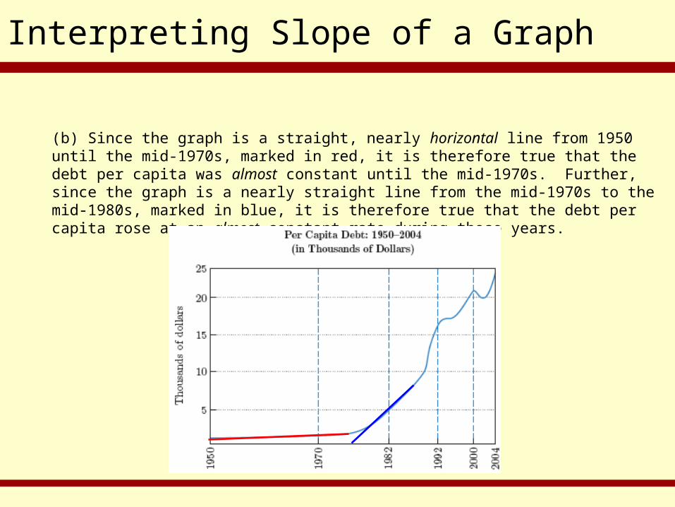
Refer to the figure below to decide whether the following statements about the debt per capita are correct or not. Justify your answers .

(a) The debt per capita rose at a faster rate in 1980 than in 2000.

(b) The debt per capita was almost constant up until the mid-1970s and then rose at an almost constant rate from the mid-1970s to the mid-1980s.


(a) The slope of the graph in 1980 is marked in red and the slope of the graph in 2000 is marked in blue, using tangent lines. It appears that the slope of the red line is the steeper of the two. Therefore, it is true that the debt per capita rose at a faster rate in 1980.


(b) Since the graph is a straight, nearly horizontal line from 1950 until the mid-1970s, marked in red, it is therefore true that the debt per capita was almost constant until the mid-1970s. Further, since the graph is a nearly straight line from the mid-1970s to the mid-1980s, marked in blue, it is therefore true that the debt per capita rose at an almost constant rate during those years.

Equation & Slope of a Tangent Line

EXAMPLEEXAMPLE

Given the slope of the graph of y = x2 at the point (x, y) is 2x. Find the slope of the tangent line to the graph of y = x2 at the point (-0.4, 0.16) and then write the corresponding equation of the tangent line.

§ 1.3

The Derivative

The Derivative

Definition Example

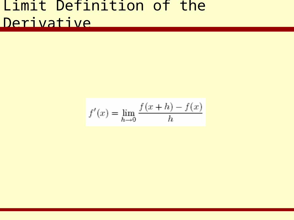
Derivative: The slope formula for a function y = f (x), denoted:

Given the function f (x) = x3, the derivative is

. xfy . 3 2xxf

Differentiation

Definition Example

Differentiation: The process of computing a derivative.

No example will be given at this time since we do not yet know how to compute derivatives. But don’t worry, you’ll soon be able to do basic differentiation in your sleep.

Differentiation Examples

These examples can be summarized by the following rule.


EXAMPLEEXAMPLE

Find the derivative of .1

7 xxf


EXAMPLEEXAMPLE

Find the slope of the curve y = x5 at x = -2.

Equation of the Tangent Line to the Graph of y = f (x) at the point (a, f (a))

Equation of the Tangent Line

EXAMPLEEXAMPLE

Find the equation of the tangent line to the graph of f (x) = 3x at x = 4.

Leibniz Notation for Derivatives

Ultimately, this notation is a better and more effective notation for working with derivatives.

Calculating Derivatives Via the Difference Quotient

The Difference Quotient is

.h

xfhxf

Differentiable

Definition Example

Differentiable: A function f is differentiable at x if

approaches some number as h approaches zero.

The function f (x) = |x| is differentiable for all values of x except x = 0 since the graph of the function has no definite slope when x = 0 (f is nondifferentiable at x = 0) but does have a definite slope (1 or -1) for every other value of x.

h

xfhxf

0

1

2

3

-3 -2 -1 0 1 2 3

Limit Definition of the Derivative

Use TI89 to Graph

I. Slope and tangent lines

1) Graph the function.

2) 2nd Draw 5, then type x value

or graph 2nd calc 6, then type x value.

II. Graph y and y’ at the same time

1) graph the function in y1.

2) Enter y2 = nDerive(y1, x, x), then graph:

y2 = Math nDerive( Vars Yvars y1 then press , x, x) graph

§ 1.4

Limits and the Derivative

Definition of the Limit

Finding Limits

EXAMPLEEXAMPLE

SOLUTIONSOLUTION

Determine whether the limit exists. If it does, compute it.

7lim 3

4

x

x

Let us make a table of values of x approaching 4 and the corresponding values of x3 – 7.

x x3 - 7 x x3 - 7

4.1 61.921 3.9 52.319

4.01 57.481 3.99 56.521

4.001 57.048 3.999 56.952

4.0001 57.005 3.9999 56.995

As x approaches 4, it appears that x3 – 7 approaches 57. In terms of our notation,

.577lim 3

4

x

x

Finding Limits

EXAMPLEEXAMPLE

SOLUTIONSOLUTION

For the following function g(x), determine whether or not exists. If so, give the limit. xgx 3

lim

We can see that as x gets closer and closer to 3, the values of g(x) get closer and closer

to 2. This is true for values of x to both the right and the left of 3.

.2lim3

xgx

Limit Theorems

Finding Limits

EXAMPLEEXAMPLE

Use the limit theorems to compute the following limit.

x

xxx 38

365lim

2

9

Limit Theorems

Finding Limits

EXAMPLEEXAMPLE

Compute the following limit.

x

xxx 38

365lim

2

9

Using Limits to Calculate a Derivative

Limit Calculation of the Derivative

EXAMPLEEXAMPLE

Using limits, apply the three-step method to compute the derivative of the following function:

. 25.02 xxxf

Using Limits to Calculate a Derivative

EXAMPLEEXAMPLE

Use limits to compute the derivative for the function .52

1

xxf 3f

Limits as x Increases Without Bound

EXAMPLEEXAMPLE

Calculate the following limit.

30

10010lim

2

x

xx

§ 1.6

Some Rules for Differentiation

Rules of Differentiation

Differentiation

Differentiate .1

13

xx

xf

EXAMPLEEXAMPLE

Differentiation

Differentiate .1

45

xxxf

EXAMPLEEXAMPLE

The Derivative as a Rate of Change

= Slope of the tangent line at the point (a, f(a))


SOLUTIONSOLUTION

Let S(x) represent the total sales (in thousands of dollars) for month x in the year 2005 at a certain department store. Represent each statement below by an equation involving S or .

EXAMPLEEXAMPLE

S

(a) The sales at the end of January reached $120,560 and were rising at the rate of $1500 per month.

(b) At the end of March, the sales for this month dropped to $80,000 and were falling by about $200 a day (Use 1 month = 30 days).

(a) Since the sales at the end of January (the first month, so x = 1) reached $120,560 and S(x) represents the amount of sales for a given month, we have: S(1) = 120,560. Further, since the rate of change of sales (rate of change means we will use the derivative of S(x)) for the month of January is a positive $1500 per month, we have: .15001 S

(b) At the end of March (the third month, so x = 3), the sales dropped to $80,000. Therefore, sales for the month of March was $80,000. That is: S(3) = 80,000. Additionally, since sales were dropping by $200 per day during March, this means that the rate of change of the function S(x) was (30 days) x (-200 dollars) = -6000 dollars per month. Therefore, we have: .60003 S

§ 1.7

More About Derivatives

Differentiating Various Independent Variables

Find the first derivative.

EXAMPLEEXAMPLE

3221 ttT

Second Derivatives

Find the first and second derivatives.

EXAMPLEEXAMPLE

513 PPf

Second Derivatives Evaluated at a Point

Compute the following.

EXAMPLEEXAMPLE

2

242

2

43

x

xxdx

d

Marginal Cost

Marginal Cost

SOLUTIONSOLUTION

Let C(x) be the cost (in dollars) of manufacturing x bicycles per day in a certain factory. Assume C(50) = 5000 and Estimate the cost of manufacturing 51 bicycles per day.

EXAMPLEEXAMPLE

.4550 C

We will first use the additional cost formula for manufacturing 1 more bicycle per day beyond the cost of producing 50 bicycles per day. We already know it costs $5000 to produce 50 bicycles per day since C(50) = 5000. So we wish to determine how much more, beyond that $5000, it costs to produce 51 bicycles.

aCaCaC 1cost additional

5050150 CCC

45500051 C

504551 C

Therefore, we estimate the cost of manufacturing 51 bicycles to be $5045.

Marginal Revenue & Marginal Profit

Marginal Revenue

SOLUTIONSOLUTION

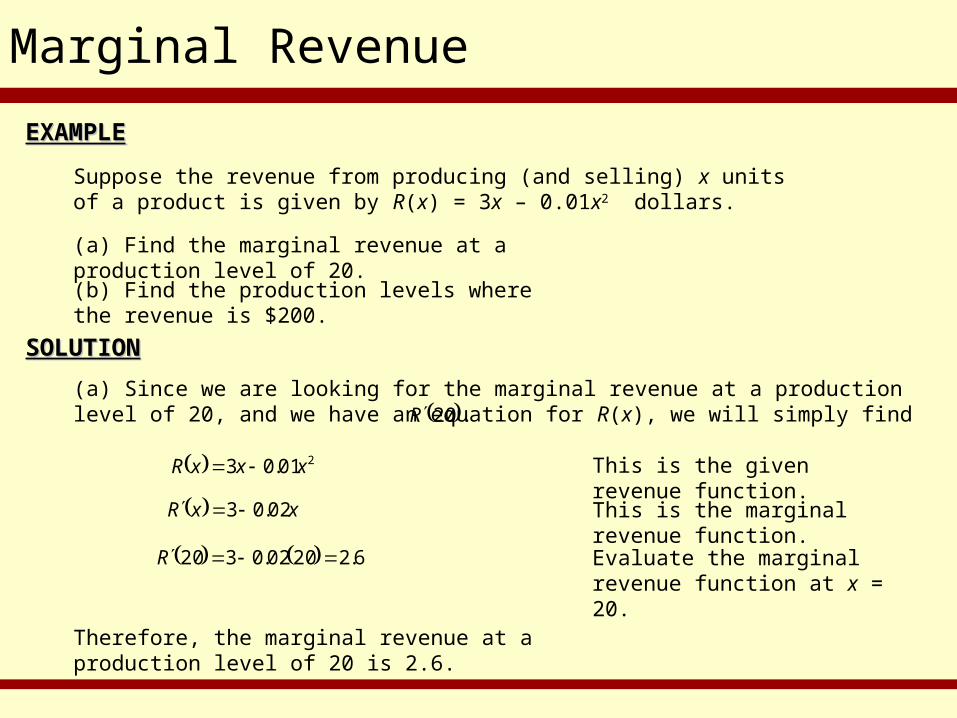
Suppose the revenue from producing (and selling) x units of a product is given by R(x) = 3x – 0.01x2 dollars.

EXAMPLEEXAMPLE

(a) Since we are looking for the marginal revenue at a production level of 20, and we have an equation for R(x), we will simply find

(a) Find the marginal revenue at a production level of 20.

(b) Find the production levels where the revenue is $200.

. 20R

201.03 xxxR This is the given revenue function.

xxR 02.03 This is the marginal revenue function.

6.22002.0320 R Evaluate the marginal revenue function at x = 20.

Therefore, the marginal revenue at a production level of 20 is 2.6.

Marginal Revenue

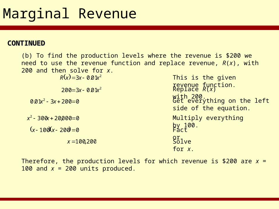
(b) To find the production levels where the revenue is $200 we need to use the revenue function and replace revenue, R(x), with 200 and then solve for x.

201.03 xxxR This is the given revenue function.

Replace R(x) with 200.

Therefore, the production levels for which revenue is $200 are x = 100 and x = 200 units produced.

CONTINUECONTINUEDD

201.03200 xx

Get everything on the left side of the equation.

0200301.0 2 xx

Multiply everything by 100.0000,203002 xx

Factor. 0200100 xx

Solve for x.200 ,100x

§ 1.8


Average Rate of Change

Average Rate of Change

Suppose that f (x) = -6/x. What is the average rate of change of f (x) over the interval 1 to 1.2?

EXAMPLEEXAMPLE

Instantaneous Rate of Change

Instantaneous Rate of Change

Suppose that f (x) = -6/x. What is the (instantaneous) rate of change of f (x) when x = 1?

EXAMPLEEXAMPLE

Average & Instantaneous Rates of Change

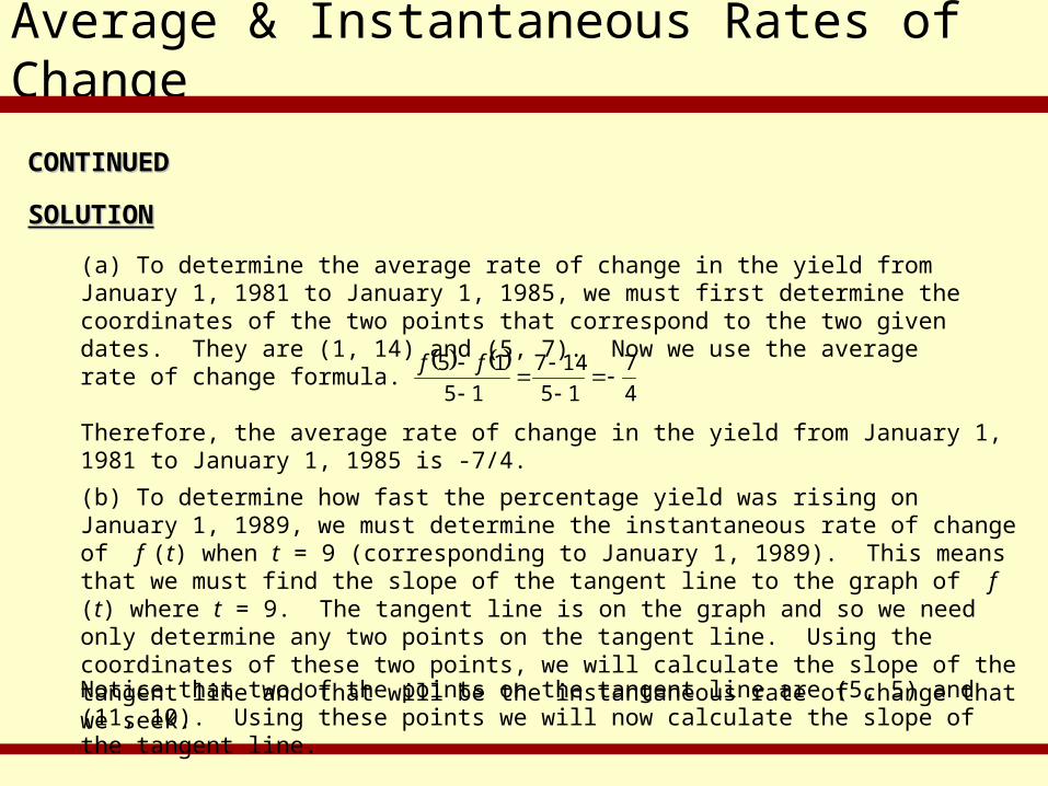
Refer to the figure below, where f (t) is the percentage yield (interest rate) on a 3-month T-bill (U.S. Treasury bill) t years after January 1, 1980.

EXAMPLEEXAMPLE

(a) What was the average rate of change in the yield from January 1, 1981 to January 1, 1985?

(b) How fast was the percentage yield rising on January 1, 1989?

(c) Was the percentage yield rising faster on January 1, 1980 or January 1, 1989?


SOLUTIONSOLUTION

4

7

15

147

15

15

ff

(a) To determine the average rate of change in the yield from January 1, 1981 to January 1, 1985, we must first determine the coordinates of the two points that correspond to the two given dates. They are (1, 14) and (5, 7). Now we use the average rate of change formula.

CONTINUECONTINUEDD

Therefore, the average rate of change in the yield from January 1, 1981 to January 1, 1985 is -7/4.

(b) To determine how fast the percentage yield was rising on January 1, 1989, we must determine the instantaneous rate of change of f (t) when t = 9 (corresponding to January 1, 1989). This means that we must find the slope of the tangent line to the graph of f (t) where t = 9. The tangent line is on the graph and so we need only determine any two points on the tangent line. Using the coordinates of these two points, we will calculate the slope of the tangent line and that will be the instantaneous rate of change that we seek.

Notice that two of the points on the tangent line are (5, 5) and (11, 10). Using these points we will now calculate the slope of the tangent line.


6

5

511

510

CONTINUECONTINUEDD

Therefore, the rate at which the percentage yield was rising on January 1, 1989 was 5/6.

(c) To determine if the percentage yield was rising faster on January 1, 1980 or January 1, 1989, we would need to know the slopes of the tangent lines corresponding to t = 0 (January 1, 1980) and t = 9 (January 1, 1989). Although we already have this information for t = 9 (see part (b)), we do not yet have this information for t = 0. Therefore, we would first need to draw a tangent line to the graph corresponding to t = 0. This is done below.


CONTINUECONTINUEDD

Obviously, finding the coordinates of two points on this tangent line might prove a little difficult. However, notice that the slopes of the two tangent lines (all we’re really interested in are their slopes) are not remotely similar (that is, the tangent lines are not close to being parallel). Therefore, in this circumstance, it would be sufficiently appropriate to notice that the blue tangent line (corresponding to t = 0) has a steeper slope and therefore the rate of change was greater on January 1, 1980 than it was on January 1, 1989.

NOTE: Use this technique of “eye-balling” a graph only when absolutely necessary and only with great care.

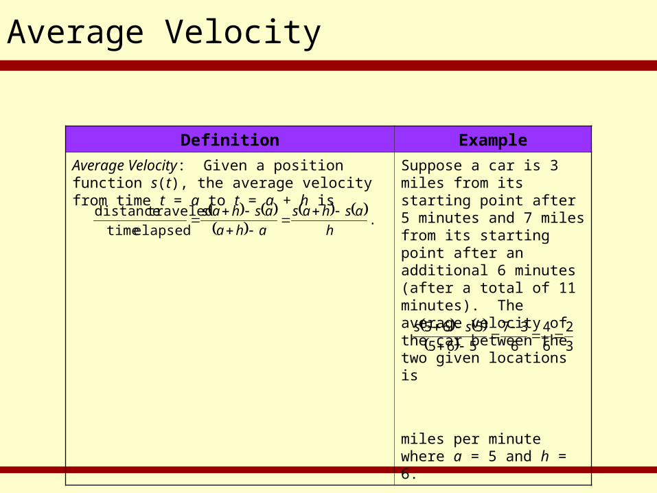
Average Velocity

Definition Example

Average Velocity: Given a position function s(t), the average velocity from time t = a to t = a + h is

Suppose a car is 3 miles from its starting point after 5 minutes and 7 miles from its starting point after an additional 6 minutes (after a total of 11 minutes). The average velocity of the car between the two given locations is

miles per minute where a = 5 and h = 6.

.

elapsed time

traveleddistance

h

ashas

aha

ashas

3

2

6

4

6

37

565

565

ss

Position, Velocity & Acceleration

s(t) is the position function, v(t) is the velocity function, and a(t) is the acceleration function.

Position, Velocity & Acceleration

A toy rocket fired straight up into the air has height s(t) = 160t – 16t2 feet after t seconds.

EXAMPLEEXAMPLE

(a) What is the rocket’s initial velocity (when t = 0)?

(b) What is the velocity after 2 seconds?

(c) What is the acceleration when t = 3?

(d) At what time will the rocket hit the ground?

(e) At what velocity will the rocket be traveling just as it smashes into the ground?

chapter 1 functions. § 1.1 the slope of a straight line

Documents