chapter 1cushman/courses/engs43/chapter1.pdfchapter 1 preliminaries 1.1 introduction objective of...
TRANSCRIPT

Chapter 1
PRELIMINARIES
1.1 Introduction
Objective of the course
Industrial activity having long reached global proportions, our natural sur-roundings have ceased to be considered inexhaustible in their resources andlimitless in their capacity to absorb the impacts of industry. No longer is itsufficient for industry to be concerned by the acquisition of raw materials, itmust be at least equally concerned by their return in modified forms to theenvironment. For example, procurement of a sufficient flow of clean water tofacilitate a chemical process may now be a lesser concern than the disposal ofthe tainted water following the process.
This generally well developed sensitivity of industry to environmental lim-itations did not, however, come easily. From initial ignorance followed by aperiod of intense antagonism between industrial leaders and self-declared envi-ronmentalists, a perception of shared responsibility for the common good hasgradually emerged. Environmental events, from minor accidents to tragic dis-asters, have brought about an inescapable realization of approaching environ-mental limits and have prompted a growing series of governmental regulations.In this context, it is imperative for scientists and engineers to be aware of thepossible environmental effects of their designs and to be prepared to modifytheir plans and activities in order to mitigate or all-together avoid those effects.While pollution avoidance is the ultimate objective, intentional and accidentalreleases of contaminants in the environment will never be eradicated. So, aserious understanding of the physics, chemistry and biology of environmentalpollution is essential.
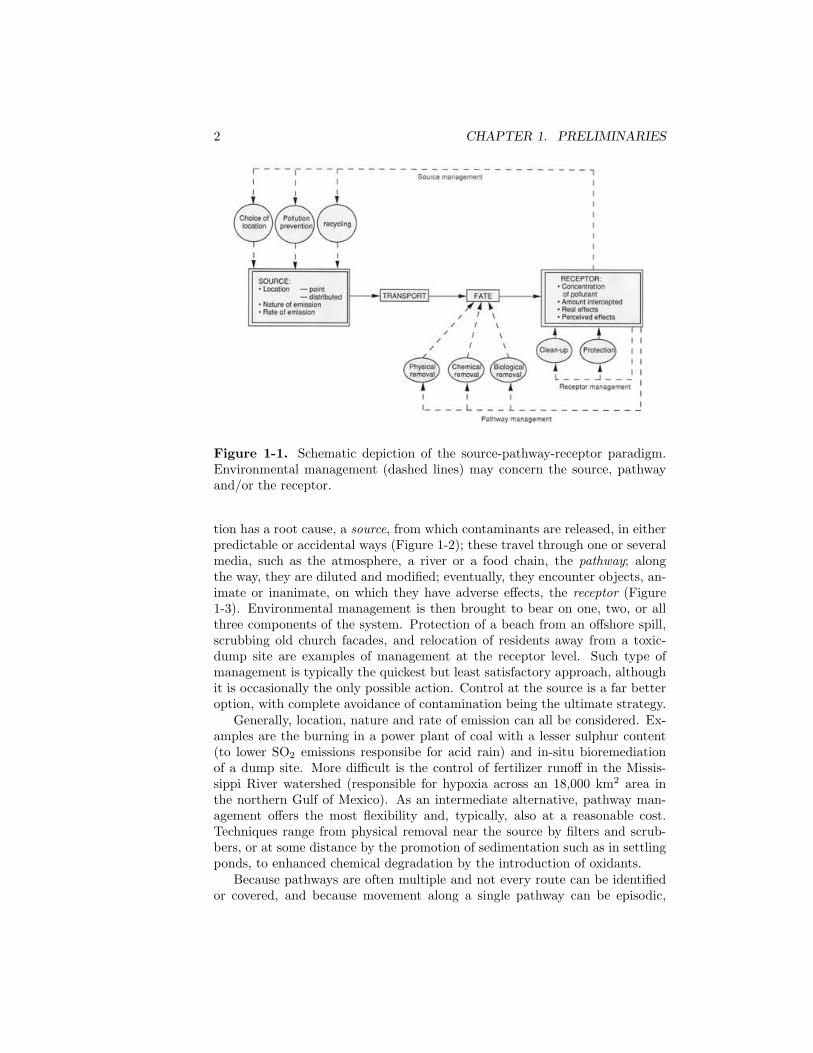
A convenient way to frame an environmental problem resulting from anyindustrial process is the source-pathway-receptor paradigm (Figure 1-1). Pollu-
1
2 CHAPTER 1. PRELIMINARIES
Figure 1-1. Schematic depiction of the source-pathway-receptor paradigm.Environmental management (dashed lines) may concern the source, pathwayand/or the receptor.
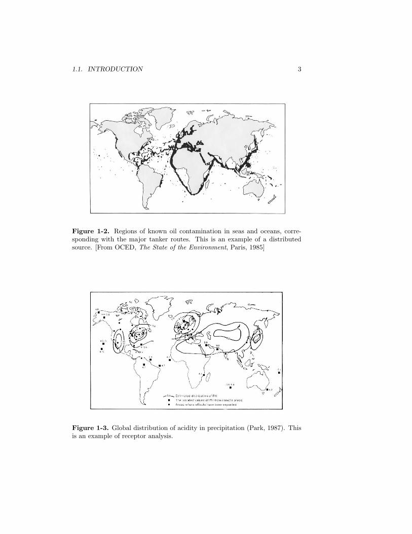
tion has a root cause, a source, from which contaminants are released, in eitherpredictable or accidental ways (Figure 1-2); these travel through one or severalmedia, such as the atmosphere, a river or a food chain, the pathway; alongthe way, they are diluted and modified; eventually, they encounter objects, an-imate or inanimate, on which they have adverse effects, the receptor (Figure1-3). Environmental management is then brought to bear on one, two, or allthree components of the system. Protection of a beach from an offshore spill,scrubbing old church facades, and relocation of residents away from a toxic-dump site are examples of management at the receptor level. Such type ofmanagement is typically the quickest but least satisfactory approach, althoughit is occasionally the only possible action. Control at the source is a far betteroption, with complete avoidance of contamination being the ultimate strategy.
Generally, location, nature and rate of emission can all be considered. Ex-amples are the burning in a power plant of coal with a lesser sulphur content(to lower SO2 emissions responsibe for acid rain) and in-situ bioremediationof a dump site. More difficult is the control of fertilizer runoff in the Missis-sippi River watershed (responsible for hypoxia across an 18,000 km2 area inthe northern Gulf of Mexico). As an intermediate alternative, pathway man-agement offers the most flexibility and, typically, also at a reasonable cost.Techniques range from physical removal near the source by filters and scrub-bers, or at some distance by the promotion of sedimentation such as in settlingponds, to enhanced chemical degradation by the introduction of oxidants.
Because pathways are often multiple and not every route can be identifiedor covered, and because movement along a single pathway can be episodic,
1.1. INTRODUCTION 3
Figure 1-2. Regions of known oil contamination in seas and oceans, corre-sponding with the major tanker routes. This is an example of a distributedsource. [From OCED, The State of the Environment, Paris, 1985]
Figure 1-3. Global distribution of acidity in precipitation (Park, 1987). Thisis an example of receptor analysis.

4 CHAPTER 1. PRELIMINARIES
management must be preceded by a careful analysis of both the transportingmechanisms and the transformations that can occur along the way. Anotherand more important reason to study pathways is to understand or be able toquantify the beneficial effect on a certain receptor following a source reductionsomewhere upstream. It is, indeed, a relatively common problem in environ-mental regulations to formulate policies and new regulations to control sourcesin order to obtain a certain level of amelioration at specified receptors. An ex-ample is the decision whether to regulate more strictly stationary power plantsor road vehicles to obtain the greatest reduction in ozone-induced lung cancersin a certain region with the least economic burden. For this, the pathwaysneed to investigated from each source to relate emission rates to ozone concen-trations over the concerned area. Such pathway analysis is the object of thiscourse in environmental transport and fate. The expression “EnvironmentalTransport and Fate” consists of three key words taken with specific meanings.
The adjective ENVIRONMENTAL refers, obviously, to our planet Earth,which consists of several systems (Figure 1-4). A natural way to distinguishthose systems is by their matter: atmosphere (air, water vapor and other gases),hydrosphere (liquid water in the sea and on land), cryosphere (ice in glaciersand on the sea), lithosphere (soils and rocks), and biosphere (all life forms).Since fluids are the only significant carriers of substances affecting the qualityof our surroundings and since the atmosphere covers 100% and the oceans 71%of the earth’s surface, the adjective ‘environmental’ will be restricted here toinclude only the atmosphere and hydrosphere. [There are important cases,however, that fall outside of this scope such as diffusion of heavy metals in soiland migration of heavy metals up the food chain.]
The noun TRANSPORT addresses the questions: How do things travel?Where do they go? Here, the emphasis is on the motion, and principles ofphysics are invoked to determine the nature of ambient motions. Typical modesof transport are prevailing winds, weather systems, the coastal sea breeze, watercurrents of all kinds, gravitational settling, and buoyant rise. The situation isgreatly complicated by the seasonal, diurnal, tidal and possible other variabilityof the transporting flow as well as by the ubiquitous presence of turbulence inenvironmental fluids.
Finally, the noun FATE refers to: What do substances become? It drawsattention to change and implicates chemistry, biology and, occasionally, nuclearphysics. Typically, a contaminant in the environment ceases to pollute when ithas been digested by biological processes, when it has chemically reacted intoharmless products, when it has decayed by radioactive reactions to levels belowthose harmful, or when it has been diluted to benign levels.
Imagine for a moment that there were no transport process whatsoever;then, contaminant levels would increase without bound right at the source.Quickly, the situation would become intolerable. In particular, we humanswould rapidly suffocate in our own exhaust of carbon dioxide. In a separatethought process, imagine now that there were no change process by which pol-lutants decay; their global concentrations would increase ceaselessly, eventuallyleading again to a scenario of ultimate suffocation. In other words, transport

1.1. INTRODUCTION 5
Figure 1-4. Depiction of the primary media of our environment: atmosphere,surface water, and subsurface (soil and groundwater). Because few substancesare confined to a single medium, exchanges between media must often be con-sidered. [Cartoon from Hemond & Fechner Chemical Fate and Transport in
the Environment, 1994]
and fate processes are vital to our well-being.
In summary, we shall study motions of substances in the air and water onour planet and investigate what happens to them along the way. In a first,preparatory stage, we will develop the physical and mathematical frameworknecessary for subsequent quantitative analyses of specific situations. The for-mulation relies primarily on a mathematical representation of the diffusion pro-cess and on budget statements. Then, in a second part, problems of transportand fate in water will be considered systematically, from rivers and aquifersto lakes, estuaries and the ocean. Finally, the third and last part covers airpollution from small to large scales (local, urban, regional, continental andglobal).
Contamination and pollution
Although most people do not make a distinction between CONTAMINA-TION and POLLUTION, it is helpful to make one in the context of envi-ronmental transport and fate. It is general practice to reserve the word con-tamination for the introduction or presence in the environment of an aliensubstance (or energy level) without implication of any adverse effect. Pollu-tion, by contrast, refers to the potential or actual damage or harm caused bythe presence of an alien substance in the environment. Thus, contaminationcharacterizes the source, while pollution relates to the receptor. It may thushappen that a contaminant does not pollute, such as when it is diluted to be-

6 CHAPTER 1. PRELIMINARIES
nign levels or transformed into harmless substances along the pathway. Viceversa, there exist natural pollutants, such as terpene and other volatile organiccoumpounds (VOCs for short) emanating from pine trees, which can contributeto atmospheric ozone formation. Another example is groundwater arsenic inBangladesh.
TOXICITY is defined as the capacity of a pollutant to cause serious harmto, or even death of, people or animals. Most pollutants are only toxic beyonda certain minimum concentration. An example is Zinc, a heavy metal thatis essential to life functions but becomes toxic at levels significantly elevatedabove natural levels. Other heavy metals, such as Cadmium, are always toxiceven at low concentrations. Therefore, in dealing with toxic or potentially toxicsubstances, it is imperative to define a level of toxicity. A pratical definition isthe dose required to kill just one organism in a given population. Then, effortsmust be made to keep the actual dose below a pre-accepted fraction of thistoxic dose.
In practice, it is generally useful to distinguish between POINT SOURCESand DISTRIBUTED SOURCES. In the case of a point source, we can identifya single location of contaminant release (example: one smokestack, Love Canal,Fukushima reactor No. 1), while we cannot do so for distributed sources (ex-amples: traffic in Los Angeles, agricultural use of pesticides in the Midwest).Because remediation of pollution caused by distributed sources is a much harderproblem, a significantly greater amount of effort over the years has concentratedon remediation of pollution by point sources. But, this fact does not diminishin any way the importance of problems caused by distributed sources. Smogover Los Angeles, acid precipitation over New England lakes, and stratosphericozone depletion are all serious problems caused by distributed sources.
Another useful way of categorizing various kinds of contamination is bytheir source type, as shown in Table 1-1. Note that, as we proceed down thetable, we encounter problems of increasing length scale.
Finally, it is worth noting that pollution is not an additive process. Thecombination of certain substances may occasionally cause a greater harm thanthe sum of their individual effects. This situation is called SYNERGISM. Itsopposite, the case when several contaminants partially negate the effects ofone another, is called AMELIORATIVE INTERACTION. An example of syn-ergism is the dissolution by acid precipitation (caused by the combustion ofsulphur-laden fossil fuels and causing acidification of lakes) of metals fromsoils, where their previous lack of mobility rendered them much less harmful.By contrast, an example of ameliorative interaction is the so-called scavengingof ground-level ozone (where it can cause damage to vegetation) by nitrogendioxide (a bronchial irritant and precursor of nitric acid), up to a certain pointbecause of an existing chemical equilibrium between nitrogen oxides (NOx),oxygen (O2) and ozone (O3) in sunlight.
Scales
Environmental problems change character with their length scale, requiring

1.1. INTRODUCTION 7
SOURCE EXAMPLES OF SUBSTANCE
Individual Cigarette smoke,Leaking septic tank
Corporate Smokestack fumes,Tainted discharge in nearby stream
Urban Auto emissions,Smog-causing chemicals
Regional Agricultural herbicides and pesticides,Major oil spills
Continental Sulfur dioxide causing acid rain,Radioactive fallout from Chernobyl and Fukushima
Global Carbon dioxide from industrial activities,Ozone-destroying chemicals (CFCs)
Table 1-1. One possible classification of pollution sources.
different approaches for their investigation and solution depending on the scaleunder consideration. The shortest scale with which to reckon is the atomic-molecular level; at that level, one considers elementary processes such as nuclearand chemical reactions, and advances in knowledge proceed from the studyof the nature (stoichiometry) and rate (kinetics) of these reactions. The nextshortest scale of interest is the level of a single organism, where one investigates,and occasionally utilizes, biological processes. It is not unusual to have to seeksimplified descriptions of the processes at these lowest levels in order to limitthe scope of the problem under study and so permit investigations at largerscales.
The next scale of interest is the local level, where pollutants no longerappear as distinct units and where their quantity is best measured in termsof concentrations in a continuous fluid. At the local level, the focus is on flowand diffusion in the vicinity of a single source, such as an industrial smokestackor a municipal-waste discharge along a river. One then talks about near-fielddistributions.
At the urban and rural levels, individual sources are no longer separatelyidentified but are represented as a continuously distributed source. The ap-proach consists in aggregating the effects of individual sources by lumping theirnear-field properties. Daily variations may play a significant role.
At the regional and continental levels, the aggregation process is carriedone step further, and one now considers distributions of distributed sources (acity becomes a point source, and a region a continuous distribution of suchsources). The emphasis is on far-field and long-term effects. Spatial and tem-poral variability of the carrying fluid flow usually plays an important role (e.g.,
8 CHAPTER 1. PRELIMINARIES
weather patterns, seasonal aspects).Finally, the largest scale of all is the global level. Since there is no exit from
our terrestrial system, attention is drawn to cumulative aspects and conser-vation laws. At this level, atmospheric, hydrospheric and biological processesare greatly intertwined, and all successful approaches are necessarily interdis-ciplinary. Study of climate change obviously falls in this category.
Scientific approaches
In the face of the many unknowns related to environmental processes, thebest strategy is to work on all possible fronts and to check results obtained withone approach against those obtained with another. Therefore, all traditionalscientific approaches are being utilized.
OBSERVATION: In-situ measurements provide primary data, some ‘harder’(undeniable facts) and some ‘softer’ (indirect and resulting from some under-lying assumptions). Monitoring is essential in numerous situations both todiscern problems and to enforce compliance. Typical limitations are lack ofpast records, spotty coverage, instrumental shortcomings (not everything ismeasurable), and instrumental errors (imprecise data).
EXPERIMENTATION: Generation of data in specific test cases is possible,but only to a very modest extent in environmental studies. Limitations areour fundamental inability to experiment with planet Earth. Exceptions to therule are local tracer-release experiments. Reduced-scale experimentation in thelaboratory can be particularly instructive, especially in the study of chemicalreactions (fate aspects), but such experimentation may be difficult and maynot always be representative of the real world.
THEORY: Derivation of useful formulas can proceed from basic conceptsand ideas, but mathematical analysis requires simplifications, and resulting for-mulas are of limited use in often complex situations. The underlying conceptsand assumptions may also be incorrect.
SIMULATION: The use of computers to simulate complex systems is apractical way to ‘experiment’ (by changing parameters and conditions of theproblem) and is at the present time the most fruitful approach to environmentalstudies. Since it is not possible to make measurements around a facility thathas not yet been constructed, modeling is about the only way to estimatefuture impacts. Limitations reside in the inherent nature of computer modeling,namely the a-priori selection of processes retained in the formalism and thechoice of ways to model these. Thus, models remain very simplified versionsof nature, and their predictions, however realistic they may appear, are notalways correct or accurate.
In addition to the limitations of every single approach, we always have tobe mindful of other, inherent limitations: There will always remain unknownsabout pollution sources (spatial and temporal variability in distributions aswell as variations in levels), and environmental systems (atmosphere, rivers,lakes and oceans) are subject to continuous natural variability (such as diurnal,seasonal and longer climatic variations).

1.2. DEFINITIONS 9
The solution of environmental problems most often calls upon several tra-ditionally separated fields of science. While meteorology, hydraulics, limnology(study of lakes) and oceanography may be invoked for the determination oftransport mechanisms in air and water, geochemistry and biochemistry arenecessary to evaluate the fate processes. Statistics play an essential role in theassessment of problems and the evaluation of remediation strategies, while en-gineering can provide the numerical expertise, propose optimization methods,and lead to the development of new monitoring instruments and remediationtechniques. An interdisciplinary approach and a system outlook are clearlynecessary.
1.2 Definitions
We now proceed with the introduction of concepts and quantities that formthe tools for a quantitative representation of environmental transport-and-fateproblems.
Concentration
The concentration of a substance, such as sulphur dioxide SO2, is definedas the quantity of the substance per unit volume of fluid containing it:
concentration = c =quantity of substance
volume of fluid=
m
V. (1.1)
The ‘quantity’ of the substance is usually taken as the mass of substance inthe volume of fluid considered. In that case, the dimension of c is mass pervolume, or M/L3; the metric units are kg/m3. Sometimes, the quantity maybe expressed in number of atoms (radionuclides) or in mass of one of the com-ponents (e.g., grams of sulphur in a sulphur compound).
When water is the ambient fluid, concentration is often expressed in molesof the substance per liter (1L = 10−3m3) of solution. One mole comprises6.02 × 1023 atoms or molecules of that substance. The advantage of usingmolarity is the ease of translation from chemical reactions at the molecularlevel to mass budgets at the macroscopic scale: one molecule simply becomesone mole. To convert moles into grams, one multiplies by the molecular weightof the substance. [Example: The mass of 1 mole of ammonia (NH3) is 14+3×1= 17 g.]
In air, which is compressible, concentrations may change not because themass of the contaminant varies but because the volume of air containing itis modified by a pressure change. To avoid possible ambiguities (in reportingobservations or in setting maximum permissible values, for instance), it is goodpractice to express concentrations in moles of substance per mole of air, inpartial pressure, or in mass of substance per mass of air. Similarly, in dealingwith soils, which are subject to compaction and a varying level of moisture, it
10 CHAPTER 1. PRELIMINARIES
is preferable to express concentrations in mass of substance per mass of drysoil.
The evaluation of the ratio quantity-per-volume requires the choice of somevolume, over which the count is performed. This automatically translates intoaveraging over this volume. If the volume is chosen too small, irrelevant statis-tical variations arise in the count, which lead to unnecessary and undesirablenoise, while if the volume is chosen too large, information is lost by excessivesmoothing over space. Therefore, the chosen volume should be neither toosmall or too large. In practice, it should be substantially smaller than the do-main under consideration but larger than the small-scale turbulent fluctuationsleft unresolved.
Similarly, the definition of a concentration implicitly requires a temporal av-erage, because of statistical variations (molecular, turbulent, diurnal, seasonal)that are not always pertinent to the problem at hand. Again, the durationimplied by the averaging should be neither too long (at the risk of glossingover significant temporal variations) or too short (with unwanted fluctuationscomplicating the problem).
If there are several constituents or if one substance is present under severalspecies, we introduce one concentration for each:
constituent i → ci =mi
V, i = 1, 2, ...
Flux
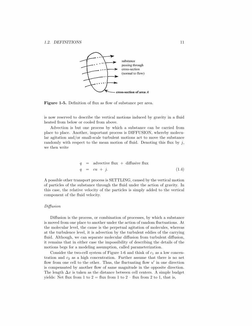
We define the flux of a substance in a particular direction as the quantityof that substance passing through a section perpendicular to that direction perunit area and per unit time (Figure 1-5):
flux = q =quantity that passes through cross-section
cross-sectional area × time duration=
m
A∆t. (1.2)
If the quantity is a mass, then the flux q is a rate of mass per area per time,and its dimensions are ML−2T−1; the metric units are kg/m2s.
Obviously, the amount of substance traversing the cross-section over whichthe count is performed depends on the nature of the transporting process. Ifthis process is the passive entrainment of the substance by the carrying fluid,then the flux can be easily related to the substance concentration and the fluidvelocity, as follows:
q =quantity
volume of fluid×
volume of fluid
area × time= cu, (1.3)
where u is the entraining fluid velocity. [Using (1.1) and (1.2), check the di-mensional consistency of equation (1.3).] This process is called ADVECTION,a term that simply means passive transport by the containing fluid. In FluidMechanics, this process used to be called convection, but the latter designation
1.2. DEFINITIONS 11
Figure 1-5. Definition of flux as flow of substance per area.
is now reserved to describe the vertical motions induced by gravity in a fluidheated from below or cooled from above.
Advection is but one process by which a substance can be carried fromplace to place. Another, important process is DIFFUSION, whereby molecu-lar agitation and/or small-scale turbulent motions act to move the substancerandomly with respect to the mean motion of fluid. Denoting this flux by j,we then write
q = advective flux + diffusive flux
q = cu + j. (1.4)
A possible other transport process is SETTLING, caused by the vertical motionof particles of the substance through the fluid under the action of gravity. Inthis case, the relative velocity of the particles is simply added to the verticalcomponent of the fluid velocity.
Diffusion
Diffusion is the process, or combination of processes, by which a substanceis moved from one place to another under the action of random fluctuations. Atthe molecular level, the cause is the perpetual agitation of molecules, whereasat the turbulence level, it is advection by the turbulent eddies of the carryingfluid. Although, we can separate molecular diffusion from turbulent diffusion,it remains that in either case the impossibility of describing the details of themotions begs for a modeling assumption, called parameterization.
Consider the two-cell system of Figure 1-6 and think of c1 as a low concen-tration and c2 as a high concentration. Further assume that there is no netflow from one cell to the other. Thus, the fluctuating flow u′ in one directionis compensated by another flow of same magnitude in the opposite direction.The length ∆x is taken as the distance between cell centers. A simple budgetyields: Net flux from 1 to 2 = flux from 1 to 2 – flux from 2 to 1, that is,

12 CHAPTER 1. PRELIMINARIES
Figure 1-6. Two-cell system illustrating diffusion as uneven exchange.
j = c1 u′− c2 u′
= − u′∆c,
where ∆c = c2 – c1 is the concentration difference. Multiplying and dividingby ∆x and taking the limit toward infinitely small distances, we obtain:
j = − (u′∆x)∆c
∆x
and then
j = − Ddc
dx, (1.5)
where D is equal to the limit of the product u′∆x as ∆x becomes small and iscalled the diffusion coefficient, or DIFFUSIVITY. [Dimensions are L2T−1, andmetric units are m2/s.]
Thus, we see that the diffusive flux of substance is proportional to thegradient of the concentration. In retrospect, this makes sense; if there wereno difference in concentrations between cells, the flux from one into the otherwould be exactly compensated by the flux in the opposite direction yielding novisible transfer. It is the concentration difference (the gradient) that matters.Further, the greater the concentration difference, the larger the imbalance offluxes, and thus the net flux increases with the gradient.
Equation (1.5) is called Fick’s law of diffusion and is analogous to Fourier’slaw of heat conduction. (Heat flows from hot to cold with a flux equal toa conductivity coefficient times the temperature gradient.) The expression‘Fickian diffusion’ is sometimes used to imply relation (1.5).
Diffusion is ‘down-gradient’, that is the transport is from high to low con-centrations. (In the preceding example with c1 < c2, j is negative and the net

1.3. MASS BALANCE 13
flux is from cell 2 to cell 1.) This implies that the concentration increases on thelow side and decreases on the high side, and the two concentrations will grad-ually become equal. Once they are equal (dc/dx = 0), diffusion stops althoughrandom fluctuations never cease. Therefore, diffusion acts toward homogeniza-tion of the substance, just as heat diffusion tends to render the temperatureuniform.
The pace at which diffusion proceeds depends critically on the value ofthe diffusion coefficient D. This coefficient is inherently the product of twoquantities, a velocity (u′) and a length scale (∆x), measuring respectively themagnitude of the fluctuating motions and their range. For molecular agitation,u′ is the thermal velocity uT of Brownian motion, a function of the temperatureof the medium, and ∆x is the mean free path l between consecutive collisions.So, Dmolecular = uT l. In a turbulent fluid, u′ is the typical eddy orbital velocityu∗, and ∆x is the mean eddy diameter d, yielding Dturbulent = u∗d. Becauseturbulence is typically much stronger than molecular agitation (chiefly becaused ≫ l), Dturbulent is much larger than Dmolecular, and in environmental ap-plications in which turbulence is ubiquitous, attention must always be paidto the turbulence of the containing fluid rather than to molecular diffusion.This situation is quite unfortunate since turbulence is an unsolved problem ofphysics. A particularly acute complication is the fact that the turbulent activ-ity varies enormously in space (smaller-scale turbulence near ground and walls,and larger-scale turbulence in the interior of a system or in a jet).
1.3 Mass Balance
Control-volume budget
Because “everything has to go somewhere”, we should account for the entireamount of any substance in the system. The first question is: What do we doa budget for? The second question is: Where do we perform the budget? Andso, we carefully state which substance we track (e.g. sulphur in all forms orspecifically in the SO2 form) and define a control volume, such as a piece ofequipment, a power plant, a lake, a city, the entire planet, etc. This controlvolume may be almost anything but must be clearly defined, so that we knowunambiguously whether something is inside it or outside it, and it ought to bepractical, so that the resulting budget will yield valuable information.
We treat the control volume as a ‘bulk’ object, i.e. we do not distinguishseparate portions of the system therein and assign a single or ‘mixed’ concen-tration c to the entire volume V of the fluid within the control volume. Ifthis lumping is unsatisfactory, it is then necessary to define a series of smallercontrol volumes and perform a separate budget analysis for each one.
For a single control volume (Figure 1-7), the budget is, naturally:
Accumulation over time = Σ Imports through sides

14 CHAPTER 1. PRELIMINARIES
Figure 1-7. A schematic control volume for a mass budget.
− Σ Exports through sides
+ Σ Interior sources
− Interior decay.
Usually, the budget is written as a rate (that is, per time). The accumulationis then the difference between the amounts present in the control volume atthe later time t+∆t and the earlier time t, divided by the time lapse ∆t:
Accumulation over time =1
∆t[(cV )t+∆t − (cV )t].
In the limit of an infinitesimal time lapse:
Accumulation over time =d
dt(cV )
= Vdc
dt,
since the volume V is unchanging in time. Cases with temporally varyingvolumes can be treated, but these are extremely rare in environmental appli-cations. [Check the dimensions: Volume × concentration (= mass per volume)per time = mass per time.]
For a lumped control volume, we may neglect the diffusive flux, retainingonly advection by the surrounding fluid:
j = 0 → q = cu,
and the sum of imports through the sides (inlets) of the system is:

1.3. MASS BALANCE 15
Σ Imports through sides = Σ qin Ain
= Σ cin uin Ain
= Σ cin Qin,
where the sum covers all inlets, uin is the entering fluid velocity, cin the con-centration of the substance at the entrance location, Ain is the cross-sectionalarea of the inlet, and Qin = uinAin is the entering flux of the carrying fluid.[Check the dimensions of each product cuA: concentration (= mass per lengthcubed) × velocity (= length per time) × area (= length squared) = mass pertime.] Similarly, the sum of exports is expressed as:
Σ Exports through sides = Σ qout Aout
= Σ cout uout Aout
= Σ cout Qout,
with analogous interpretations for the various factors. But, one additionalstatement can be made: The exit concentration must be that of the mixed con-dition inside the volume and thus be the same at all outlets, noted c. Therefore,
Σ Exports through sides = (Σ Qout) c.
There is one exception to this last simplification: Evaporation. If the budgetis written for a body of water exposed to the atmosphere and one of the path-ways by which water leaves the system is evaporation along the surface, theoutgoing flux is one of pure (distilled) water, and the accompanying outgoingconcentration is zero.
In most cases, the carrying fluid can be assumed incompressible and con-served. There is then no loss or gain of fluid volume, and the total volumetricflow rate of entering fluid must be equal to that leaving the system, and wecan write:
Σ Qout = Σ Qin.
The specification of the rate of decay inside the volume requires a knowledgeof the decay mechanism(s) such as chemical reactions. But, in general, therate of decay can be reasonably assumed to be proportional to the amount ofsubstance present in the system. After all, in well mixed conditions, the moremolecules are present, the more chemical reactions occur per unit time. Sincethe total amount of substance present in the system is cV (from the definitionof c), we state:
Interior decay = KcV,
in which K is a constant representing the rate at which decay proceeds. Thedimension of K is one over time, so that the dimension of KcV is again mass
16 CHAPTER 1. PRELIMINARIES
per time. The time 1/K can be interpreted as the ‘lifetime’ of the substancein the control volume.
Finally, the contribution of all sources requires detailed knowledge of themechanism(s) producing the substance in the system. For example, the sub-stance being tracked may be the product of a chemical reaction taking placeinside the control volume. For lack of further specification, we will write fornow:
Σ Interior sources = S,
in which the quantity S is simply the total mass of the substance producedwithin the system per unit time.
Putting it all together, we obtain the following mass budget for the sub-stance under consideration:
Vdc
dt= − (Σ Qout + KV ) c+ Σ Qin cin + S. (1.6)
Typically, the concentration c of the substance in the control volume is un-known, while all other quantities are given, so that (1.6) is the equation gov-erning the evolution of c over time.
Particular cases
a) STEADY STATE: If the system is in equilibrium, the concentration of thesubstance is unchanging with time (there is no accumulation/depletion), i.e.dc/dt = 0. Equation (1.6) then becomes
(Σ Qout + KV ) c = Σ Qin cin + S,
and can be immediately solved for c:
c =Σ Qin cin + S
Σ Qout + KV. (1.7)
b) CONSERVATIVE SUBSTANCE: There is neither source nor decay, i.e.
S = K = 0. Equation (1.6) reduces to
Vdc
dt= − (Σ Qout) c + Σ Qin cin. (1.8)
c) STEADY STATE & CONSERVATIVE SUBSTANCE: dc/dt = S = K = 0and
c =Σ Qin cinΣ Qout
. (1.9)
d) ISOLATED SYSTEM: There is no exchange with the exterior, leaving onlythe internal terms:

1.3. MASS BALANCE 17
Vdc
dt= − KV c + S. (1.10)
If moreover the source S is constant over time and the initial concentrationis c(t = 0) = c0, the solution is
c =S
KV+
(
c0 −S
KV
)
e−Kt, (1.11)
and the concentration varies gradually from its initial value to the ultimatevalue
c∞ =S
KV(1.12)
(higher or lower than c0), which represents an equilibrium. At this equilibrium,the rate of production is balanced by the rate of decay (S = KV c at c = c∞).The decay-rate constant K not only determines the ultimate concentration c∞but also the rapidity at which the system equilibrates. The system is ‘half-waythere’ when
c =1
2(c0 + c∞)
and this occurs at time t50% such that
exp(−Kt50%) =1
2or
t50% =ln 2
K=
0.693
K. (1.13)
As it is evident from the definition of decay-rate coefficient K, the larger K,the quicker the system tends toward equilibrium.
Example (adapted from G.M. Masters, 1997, pp. 10-14)
A bar with an air volume of 500 m3 is ventilated at the rate of 1000 m3/hr(Figure 1-8). When the bar opens at 5pm, its air is pure and 50 smokers enter,each starting to smoke two cigarettes per hour. An individual cigarette emits,among other things, about 1.40 mg of formaldehyde, a toxin that converts tocarbon dioxide at the rate K = 0.40/hr. Estimate the formaldehyde concen-tration at 6pm and 7pm and the steady-state concentration. If the thresholdfor eye irritation is 0.06 mg/m3 at what time does the smoke begin to irritatethe occupants’ eyes?
We solve this problem by determining first the source of formaldehyde
S = 1.4mg
cigarette× 2
cigarettes
smoker× hour× 50 smokers = 140
mg
hour.
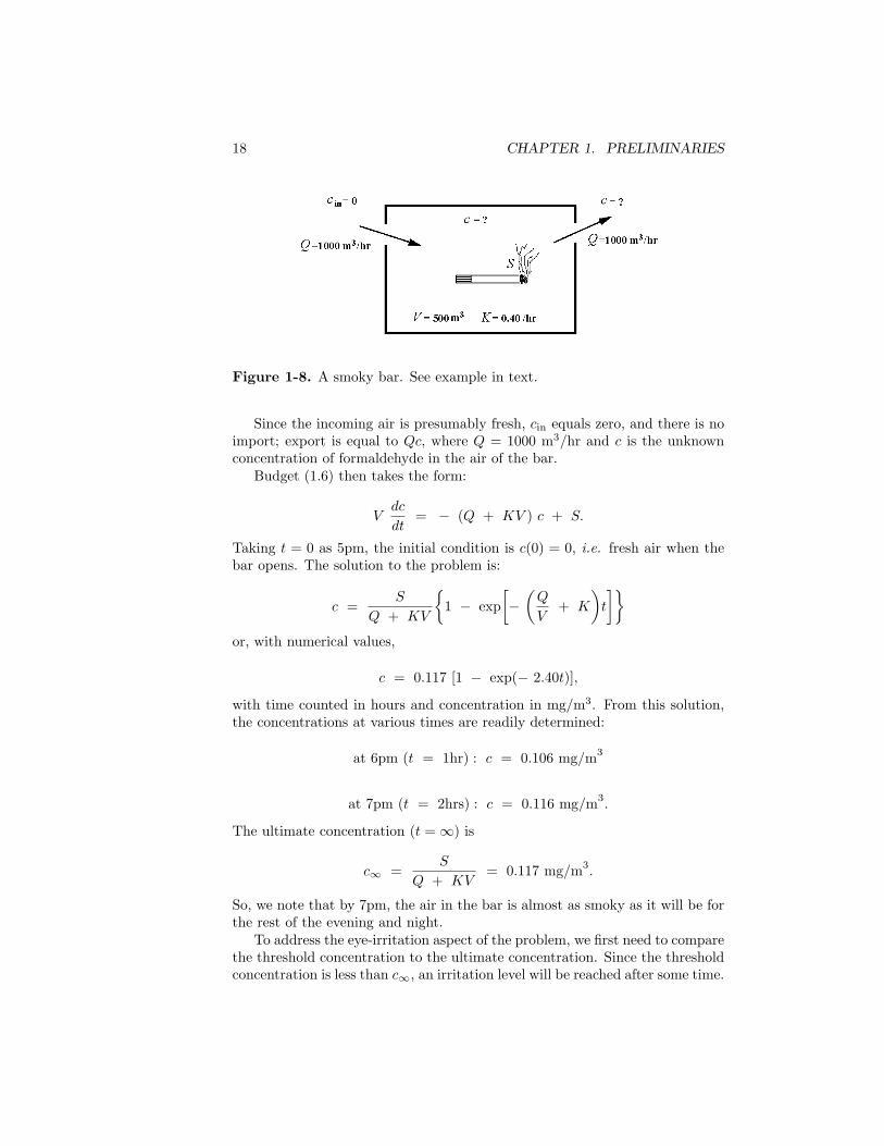
18 CHAPTER 1. PRELIMINARIES
Figure 1-8. A smoky bar. See example in text.
Since the incoming air is presumably fresh, cin equals zero, and there is noimport; export is equal to Qc, where Q = 1000 m3/hr and c is the unknownconcentration of formaldehyde in the air of the bar.
Budget (1.6) then takes the form:
Vdc
dt= − (Q + KV ) c + S.
Taking t = 0 as 5pm, the initial condition is c(0) = 0, i.e. fresh air when thebar opens. The solution to the problem is:
c =S
Q + KV
{
1 − exp
[
−
(
Q
V+ K
)
t
]}
or, with numerical values,
c = 0.117 [1 − exp(− 2.40t)],
with time counted in hours and concentration in mg/m3. From this solution,the concentrations at various times are readily determined:
at 6pm (t = 1hr) : c = 0.106 mg/m3
at 7pm (t = 2hrs) : c = 0.116 mg/m3.
The ultimate concentration (t = ∞) is
c∞ =S
Q + KV= 0.117 mg/m
3.
So, we note that by 7pm, the air in the bar is almost as smoky as it will be forthe rest of the evening and night.
To address the eye-irritation aspect of the problem, we first need to comparethe threshold concentration to the ultimate concentration. Since the thresholdconcentration is less than c∞, an irritation level will be reached after some time.

1.4. ENERGY BALANCE 19
Inverting the preceding solution, we derive the time at which the threshold isreached:
t =−1
2.40ln
(
1 −c
0.117
)
=−1
2.40ln
(
1 −0.06
0.117
)
= 0.301 hour,
that is about 18 minutes after the bar opens!It is instructive to explore what action could be taken to remediate this
situation, that is: What can be done so that the bar occupants do not sufferfrom eye irritation? Following the source-pathway-receptor paradigm, we canthink along three different directions:
• Management at the source: This could mean one of several things, suchas prohibiting the occupants from smoking or redesigning the cigarettes so thatthey no longer emit formaldehyde. A smoking ban is possible, but for businessreasons the bar owner will enforce it only if required by law. Redesigning thecigarette is not practical. As a halfway measure, the bar owner could alsoask that customers not smoke more than a certain number of cigarettes perhour, so that the ultimate concentration S/(Q +KV ) may remain under theeye-irritation threshold. Although this number can be determined (1 cigaretteper hour), it is not practical to impose and, even less, to enforce that smokersabide by this restriction.
• Management at the receptor: This could mean distributing eye googlesto the bar occupants or having them use eye drops to decrease their sensitivityto irritation. Neither is practical.
• Management of the pathway: By elimination, this offers the best hope ofsolution, short of a smoking ban. The goal can be reached in one of two ways,either increasing the ventilation rate or the size of the room. In each case, onecan ask what higher values of Q or V will make the ultimate concentrationS/(Q+KV ) fall below the threshold level of 0.06 mg/m3. For S maintained at140 mg/hr and K at 0.4 /hr, one obtains Q ≥ 2,133 m3/hr for an unchangedroom volume and V ≥ 3,333 m3 for an unchanged ventilation rate. Since it iseasier to increase the ventilation rate by 133% than the room volume by 567%,the first alternative is the better choice.
1.4 Energy Balance
Heat as a pollutant
Low-grade heat (in fluids at temperatures slightly above ambient levels) isa by-product of many industrial processes, especially power generation fromcombustion and nuclear reactions. It is usually released to the environment(atmosphere or nearby river), where it may have adverse effects, such as a
20 CHAPTER 1. PRELIMINARIES
modification of the local weather or killing of fish. Thus, heat may occasionallybe regarded as a pollutant.
Just as we can account for the mass of a pollutant, thermodynamics teachus that we should be able to account for all the energy in the system. Writingan energy budget is particularly well suited to problems involving changes intemperature and permits to track heat as a pollutant.
Control-volume budget
The first law of thermodynamics states that no energy is ever lost. Energycan only be transformed from one form to another or transported to anotherplace. Energy from chemical bonds may be released in the form of heat byexothermic reactions (e.g., combustion). Likewise, endothermic reactions actas heat sinks. While thermal engines can convert substantial amounts of heatinto electromechanical energy (e.g., gas turbine coupled to an electric gener-ator), heat generation by mechanical friction and electrical resistance (jointlycalled dissipation) are generally negligible (from the point of view of the heatbudget). If we restrict our attention to energy only in the form of heat, exother-mic chemical reactions and dissipation appear as sources, while endothermicreactions and production of electromechanical work enter the budget as sinks.Thus, a heat budget for a specific control volume can be written as follows:
Change in heat content of the control volume
= Σ Imports through sides + Σ Heat sources
− Σ Exports through sides − Σ Heat sinks,
where ‘Heat sources’ and ‘Heat sinks’ include all energy transformations be-tween heat and other forms of energy (chemical, potential, kinetic and electri-cal).
The heat content of a fluid is called internal energy and is due to the molecu-lar agitation of its molecules. Since the level of agitation increases with temper-ature, the corresponding amount of energy is taken proportional to temperatureand is expressed as
Internal energy = mCvT,
where m is the mass of fluid (in kg), Cv is its heat capacity (in joules per kgper degree), and T is its absolute temperature (in degrees Kelvin).
If the energy imports and exports consist of fluxes of various fluids at dif-ferent temperatures, we can write:
Σ Imports through sides = Σ min Cv,in Tin
Σ Exports through sides = Σ mout Cv,out Tout,

1.4. ENERGY BALANCE 21
where min and mout are the rates of mass influx and efflux per unit time(m = ρQ = fluid density times volumetric rate). The energy budget is:
Σ mi Cv,i
dTi
dt= Σ min Cv,in Tin − Σ mout Cv,out Tout + S − W,
where the subscript i refers to the various fluids present in the control vol-ume, and S and W represent respectively the heat sources and sinks (workperformed) per unit time.
If the budget is written for a single fluid, and if there is only one exit,the exit temperature may be taken as the uniform temperature within thecontrol volume. With allowance made for imports of the same fluid at varioustemperatures, the energy budget reduces to:
mdT
dt= Σ min Tin − (Σ mout) T +
S − W
Cv
. (1.14)
Recall that m = ρV and m = ρQ, where ρ is the fluid density (a function oftemperature), V is the volume of fluid present inside the control volume, andthe Q’s are the inward and outward volumetric fluxes. If the fluid density isnearly a constant (because despite their significance for the heat budget thedifferences in temperature do not affect the fluid’s density very much), Equation(1.14) can be further simplified:
VdT
dt= Σ Qin Tin − (Σ Qout) T +
S − W
ρCv
. (1.15)
Example (adapted from G.M. Masters, 1997, pp. 21-22)
A coal-fired power plant produces electrical energy with an efficiency of33.3% (Figure 1-9). The electrical power output of the plant is 1000 MW. Theother two thirds of the energy content of the fuel is released to the environ-ment as waste heat. About 15% of this waste heat goes up the smokestack(hot fumes) and the remaining 85% is taken away by cooling water, which isdrawn from a nearby river. The river has an upstream flow of 100 m3/s anda temperature of 20◦C. If the temperature of the cooling water is allowed torise only by 10◦C, what portion of the river flow needs to be diverted to thepower plant? And, what is the river temperature just downstream of where itreceives the warmer water exiting the cooling system?
To solve this problem, let us first determine how much waste heat goesinto the river. If the 1000 MW output represents only one third of the energycontent in the coal, the rate at which energy enters the power plant is
Ptotal = 3 × 1000 MW = 3000 MW.
[Note the use of the letter P since energy per time is power.] The productionof waste heat is obtained by subtraction of the electrical power output.

22 CHAPTER 1. PRELIMINARIES
Figure 1-9. A power plant releasing waste heat to both atmosphere andsurface water. See example in text.
Pwaste heat = 3000 MW − 1000 MW = 2000 MW.
Of this, 15% or 300 MW goes out by the smokestack, leaving 85% or Pwater =1700 MW to be taken up by river water.
At this stage, we write the heat budget for the river water inside the powerplant. An unknown amount Q (in m3/s) enters the plant at temperature 20◦C= 293 K and exits ten degrees warmer, at temperature 30◦C = 303 K. Insidethe plant, this water receives Pwater = 1700 MW. Budget (1.15) takes the form:
0 = Heat content of entering water − Heat content of exiting water
+ Heat from combustion,
or
0 = Q Tin − Q Tout +Pwater
ρCv
,
where Q is the unknown water flux going through the cooling system, Tin =293 K, Tout = 303K, ρ = 1000 kg/m3 is the water density (we ignore its smallchange with temperature), Cv = 4184 J/kg.K is the specific heat of water, andPwater = 1700 MW = 1700 106 J/s. Solving for Q, we obtain
Q =Pwater
ρCv(Tout − Tin)=
1.7 109
1000 × 4184 × 10= 40.63 m3/s.
Because this rate is less than the 100 m3/s available in the river, the plannedcooling system is feasible.
To determine the temperature of the downstream water, we write again anenergy budget but this time for a water volume surrounding the location where
1.4. ENERGY BALANCE 23
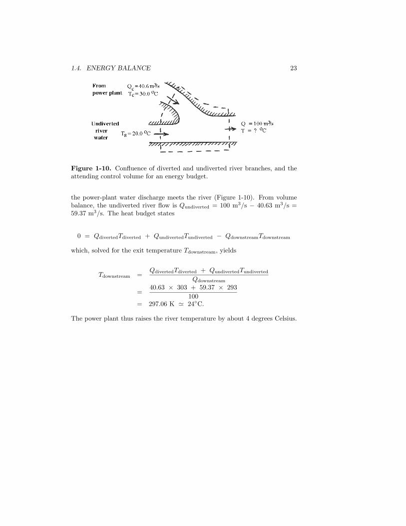
Figure 1-10. Confluence of diverted and undiverted river branches, and theattending control volume for an energy budget.
the power-plant water discharge meets the river (Figure 1-10). From volumebalance, the undiverted river flow is Qundiverted = 100 m3/s − 40.63 m3/s =59.37 m3/s. The heat budget states
0 = QdivertedTdiverted + QundivertedTundiverted − QdownstreamTdownstream
which, solved for the exit temperature Tdownstream, yields
Tdownstream =QdivertedTdiverted + QundivertedTundiverted
Qdownstream
=40.63 × 303 + 59.37 × 293
100= 297.06 K ≃ 24◦C.
The power plant thus raises the river temperature by about 4 degrees Celsius.

24 CHAPTER 1. PRELIMINARIES
Chapter 2
NEXT CHAPTER
THIS IS TO ENSURE THAT CHAPTER 1 ENDS ON AN EVEN PAGE SOTHAT CHAPTER 2 CAN BEGIN ON AN ODD PAGE.
25