Channel State Information Fingerprinting Based Indoor Localization: a Deep

Learning Approach

by

Lingjun Gao

A thesis submitted to the Graduate Faculty ofAuburn University

in partial fulfillment of therequirements for the Degree of

Master of Science

Auburn, AlabamaAugust 1, 2015

Keywords: Channel state information, deep learning, fingerprinting, indoor localization,WiFi

Copyright 2015 by Lingjun Gao

Approved by

Shiwen Mao, McWane Associate Professor of Electrical and Computer EngineeringThaddeus Roppel, Associate Professor of Electrical and Computer Engineering

Jitendra Tugnait, James B. Davis and Alumni Professor

Abstract

With the fast growing demand of location-based services in indoor environments, indoor

positioning based on fingerprinting has attracted a lot of interest due to its high accuracy. In

this thesis, we present a novel deep learning based indoor fingerprinting system using Channel

State Information (CSI), which is termed DeepFi. Based on three hypotheses on CSI, the

DeepFi system architecture includes an off-line training phase and an on-line localization

phase. In the off-line training phase, deep learning is utilized to train all the weights as

fingerprints. Moreover, a greedy learning algorithm is used to train all the weights layer-by-

layer to reduce complexity. In the on-line localization phase, we use a probabilistic method

based on the radial basis function to obtain the estimated location. Experimental results are

presented to confirm that DeepFi can effectively reduce location error compared with three

existing methods in two representative indoor environments.

ii

Acknowledgments

First of all, I would like to express my gratitude to my advisor Prof. Shiwen Mao, who

guided me throughout this thesis research and patiently helped me whenever this is a prob-

lem. I would also like to thank my thesis committee members, Prof. Jitendra Tugnait and

Prof. Thaddeus Roppel for their encouragement and insightful comments on my research.

I also would like to thank my team members, in particular, Xuyu Wang, as well as other

my friends, who gave lots of assistance throughout my thesis work. They not only helped

me to get into this new field, but also worked with me to collect experimental data during

many nights. I could not successfully complete this thesis without their support.

Finally I would like to thank my family for encouraging and supporting me with their

love and best wishes.

This work was supported in part by the US National Science Foundation (NSF) under

grant CNS-1247955, the NSF I/UCRC Broadband Wireless Access & Applications Center

(BWAC) site at Auburn University, and the Wireless Engineering Research and Education

Center (WEREC) at Auburn university.

iii

Table of Contents

Abstract . . . . . . . . . . . . . . . . . . . . . . . . . . . . . . . . . . . . . . . . . . . ii

Acknowledgments . . . . . . . . . . . . . . . . . . . . . . . . . . . . . . . . . . . . . . iii

List of Figures . . . . . . . . . . . . . . . . . . . . . . . . . . . . . . . . . . . . . . . vi

List of Tables . . . . . . . . . . . . . . . . . . . . . . . . . . . . . . . . . . . . . . . . ix

1 Introduction . . . . . . . . . . . . . . . . . . . . . . . . . . . . . . . . . . . . . . 1

1.1 Problem . . . . . . . . . . . . . . . . . . . . . . . . . . . . . . . . . . . . . . 1

1.2 Approach . . . . . . . . . . . . . . . . . . . . . . . . . . . . . . . . . . . . . 3

1.3 Layout . . . . . . . . . . . . . . . . . . . . . . . . . . . . . . . . . . . . . . . 4

2 Background . . . . . . . . . . . . . . . . . . . . . . . . . . . . . . . . . . . . . . 5

2.1 Fingerprinting-based Localization . . . . . . . . . . . . . . . . . . . . . . . . 5

2.2 Ranging-based Localization . . . . . . . . . . . . . . . . . . . . . . . . . . . 12

2.3 AOA-based Localization . . . . . . . . . . . . . . . . . . . . . . . . . . . . . 16

3 Hypotheses and Testbed Implementation . . . . . . . . . . . . . . . . . . . . . . 21

3.1 Channel State Information . . . . . . . . . . . . . . . . . . . . . . . . . . . . 21

3.2 Hypotheses . . . . . . . . . . . . . . . . . . . . . . . . . . . . . . . . . . . . 22

3.2.1 Hypotheses 1 . . . . . . . . . . . . . . . . . . . . . . . . . . . . . . . 22

3.2.2 Hypotheses 2 . . . . . . . . . . . . . . . . . . . . . . . . . . . . . . . 25

3.2.3 Hypotheses 3 . . . . . . . . . . . . . . . . . . . . . . . . . . . . . . . 25

3.3 Experiment Setup . . . . . . . . . . . . . . . . . . . . . . . . . . . . . . . . . 26

3.3.1 Hardware Implementation . . . . . . . . . . . . . . . . . . . . . . . . 26

3.3.2 System Configuration and Development . . . . . . . . . . . . . . . . . 27

3.3.3 Preparation . . . . . . . . . . . . . . . . . . . . . . . . . . . . . . . . 28

3.3.4 Installation . . . . . . . . . . . . . . . . . . . . . . . . . . . . . . . . 29

iv

3.3.5 Execution . . . . . . . . . . . . . . . . . . . . . . . . . . . . . . . . . 31

3.4 Data Processing . . . . . . . . . . . . . . . . . . . . . . . . . . . . . . . . . . 33

3.4.1 Data format . . . . . . . . . . . . . . . . . . . . . . . . . . . . . . . . 33

3.4.2 CSI Figure . . . . . . . . . . . . . . . . . . . . . . . . . . . . . . . . . 34

4 The DeepFi System . . . . . . . . . . . . . . . . . . . . . . . . . . . . . . . . . . 36

4.1 System Architecture . . . . . . . . . . . . . . . . . . . . . . . . . . . . . . . 36

4.2 Weight Training with Deep Learning . . . . . . . . . . . . . . . . . . . . . . 37

4.3 Location Estimation based on Data Fusion . . . . . . . . . . . . . . . . . . 42

5 Experiment Validation . . . . . . . . . . . . . . . . . . . . . . . . . . . . . . . . 46

5.1 Experiment Methodology . . . . . . . . . . . . . . . . . . . . . . . . . . . . . 46

5.1.1 Living Room in a House . . . . . . . . . . . . . . . . . . . . . . . . . 48

5.1.2 Computer Laboratory . . . . . . . . . . . . . . . . . . . . . . . . . . 49

5.1.3 Benchmarks . . . . . . . . . . . . . . . . . . . . . . . . . . . . . . . . 50

5.2 Localization Performance . . . . . . . . . . . . . . . . . . . . . . . . . . . . . 50

5.3 Effect of Different Parameters . . . . . . . . . . . . . . . . . . . . . . . . . . 53

5.3.1 Impact of Different Antennas . . . . . . . . . . . . . . . . . . . . . . 53

5.3.2 Impact of the Number of Packets . . . . . . . . . . . . . . . . . . . . 54

5.3.3 Impact of the Number of Packets per Batch . . . . . . . . . . . . . . 56

5.4 Impact of Varying Propagation Environment . . . . . . . . . . . . . . . . . . 58

5.5 Impact of the Size of Spot . . . . . . . . . . . . . . . . . . . . . . . . . . . . 61

6 Conclusions and Future Work . . . . . . . . . . . . . . . . . . . . . . . . . . . . 64

6.1 Summary . . . . . . . . . . . . . . . . . . . . . . . . . . . . . . . . . . . . . 64

6.2 Future Work . . . . . . . . . . . . . . . . . . . . . . . . . . . . . . . . . . . . 65

Bibliography . . . . . . . . . . . . . . . . . . . . . . . . . . . . . . . . . . . . . . . . 67

v

List of Figures

2.1 The fingerprinting based localization model. . . . . . . . . . . . . . . . . . . . . 6

2.2 The architecture of the Horus system for RSSI based fingerprinting localization. 8

2.3 The architecture of the FIFS system for CSI based fingerprinting localization. . 9

2.4 The architecture of PinLoc system for fingerprinting localization with machine

learning. . . . . . . . . . . . . . . . . . . . . . . . . . . . . . . . . . . . . . . . . 9

2.5 The architecture of zee system based on crowdsourcing localization. . . . . . . . 11

2.6 The architecture of CrowdInside system for Estimating floorplan. . . . . . . . . 12

2.7 The architecture of Travi-Navi system for navigation. . . . . . . . . . . . . . . . 13

2.8 The ranging based localization model. . . . . . . . . . . . . . . . . . . . . . . . 13

2.9 The architecture of FILA system with CSI-based ranging localization. . . . . . . 15

2.10 The architecture of acoustic-based peer assisted localization system. . . . . . . . 15

2.11 The Angle-of-Arrival Algorithm presented in wireless router with two antennas. 17

2.12 Direct path estimation with the MUSIC algorithm. . . . . . . . . . . . . . . . . 17

2.13 Illustration to refine location in CUPID with AOA-based localization. . . . . . . 18

2.14 The architecture of the Arraytrack system implemented on antenna array. . . . 19

vi

2.15 The circular SAR with rotating antenna. . . . . . . . . . . . . . . . . . . . . . . 20

3.1 CDF of the standard deviation of CSI and RSS amplitudes for 150 sampled

locations. . . . . . . . . . . . . . . . . . . . . . . . . . . . . . . . . . . . . . . . 23

3.2 Amplitudes of channel frequency responses of 50 packets measured at three dif-

ferent locations. . . . . . . . . . . . . . . . . . . . . . . . . . . . . . . . . . . . . 23

3.3 CDF of the number of channel frequency responses at 50 different locations. . . 24

3.4 Amplitudes of channel frequency response measured at the three antennas of the

Intel WiFi Link 5300 NIC (each is plotted in a different color) for 50 received

packets. . . . . . . . . . . . . . . . . . . . . . . . . . . . . . . . . . . . . . . . . 24

3.5 The DeepFi Architecture. . . . . . . . . . . . . . . . . . . . . . . . . . . . . . . 27

3.6 The Intel WiFi Link 5300 Network Interface Card. . . . . . . . . . . . . . . . . 28

3.7 The CSI from the three antennas collected from one received packet. . . . . . . 35

4.1 Weight training with deep learning. . . . . . . . . . . . . . . . . . . . . . . . . . 37

5.1 Layout of the living room for training/test positions. . . . . . . . . . . . . . . . 48

5.2 Layout of the laboratory for training/test positions. . . . . . . . . . . . . . . . . 49

5.3 CDF of localization errors in the living room experiment. . . . . . . . . . . . . . 51

5.4 CDF of localization errors in the laboratory experiment. . . . . . . . . . . . . . 52

5.5 CDF of estimated errors for different antennas. . . . . . . . . . . . . . . . . . . 54

5.6 The average execution time for different antennas. . . . . . . . . . . . . . . . . . 55

vii

5.7 The expectation and the standard deviation of estimation error for different num-

ber of packets. . . . . . . . . . . . . . . . . . . . . . . . . . . . . . . . . . . . . 56

5.8 The average execution time of position estimation for different number of packets. 57

5.9 The average running time of position estimation for different number of packets

per batch. . . . . . . . . . . . . . . . . . . . . . . . . . . . . . . . . . . . . . . . 58

5.10 The expectation and the standard deviation of estimated error for different num-

ber of packets per batch. . . . . . . . . . . . . . . . . . . . . . . . . . . . . . . . 59

5.11 CDF of correlation coefficient between 90 CSI values under this environment with

obstacles and 90 CSI values under that without obstacles. . . . . . . . . . . . . 60

5.12 CDF of the correlation coefficients between 90 CSI values when a user moves

around and 90 CSI values without human mobility. . . . . . . . . . . . . . . . . 61

5.13 CDF of correlation coefficient of 90 CSI values between two adjacent points. . . 63

viii

List of Tables

5.1 Mean errors for the Living Room and and Laboratory Experiments. . . . . . . . 50

ix

Acronym List

AGC Automatic Gain Control

AOA Angle of Arrival

AP Access Point

CD Contrastive Divergence

CDF Cumulative Distribution Function

CFR Channel Frequency Response

CSI Channel State Information

CV Coefficient of Variation

FM Frequency Modulation

FPGA Field-Programmable Gate Array

GPS Global Positioning System

GSM Global System for Mobile Communications

IMU Inertial Measurement Units

IWL Intel wireless LAN

LDPL Log Distance Path Loss

LOS Line of Sight

MIMO Multiple-input and multiple-output

ML Maximum Likelihood

NIC Network Interface Card

x

NLOS Non Line of Sight

OFDM Orthogonal Frequency-Division Multiplexing

OS Operating System

PHY Physical

RBM Restricted Boltzmann Machine

RFID Radio-frequency Identification

RSS Received Signal Strength

RSSI Received Signal Strength Indication

SAR Synthetic Aperture Radar

SDR Software Defined Radio

SNR Signal to Noise Ratio

SVD Singular Value Decomposition

TOA Time of Arrival

xi

Chapter 1

Introduction

1.1 Problem

With the proliferation of mobile devices, indoor localization has become an increasingly

important problem. Unlike outdoor localization, such as the Global Positioning System

(GPS), that has line-of-sight (LOS) transmission paths, indoor localization faces a challeng-

ing radio propagation environment, including multipath effect, shadowing, fading and delay

distortion [1,2]. In addition to the high accuracy requirement, an indoor positioning system

should also have a short estimation process time and low complexity for mobile devices.

To this end, fingerprinting-based indoor localization becomes an effective method to satisfy

these requirements, where an enormous amount of measurements are essential to build a

database before real-time position estimation.

Fingerprinting localization usually consists of two basic phases: (i) the off-line phase,

which is also called the training phase, and (ii) the on-line phase, which is also called the

test phase [3]. The training phase is for database construction, when survey data related

to the position marks is collected and pre-processed. In the on-line phase, a mobile device

records real time data and tests it using the database. The test output is then used to

estimate the position of the mobile device, by searching each training point to find the

most closely matched one as the target location. Besides such nearest estimation method,

an alternative matching algorithm is to identify several close points each with a maximum

likelihood probability, and to calculate the estimated position as the weighted average of the

candidate positions.

In the off-line training stage, machine learning methods can be used to train fingerprints

instead of storing all the received signal strength (RSS) data. Such machine learning methods

1

not only reduce the computational complexity, but also obtain the core features in the RSS for

better localization performance. K-nearest-neighbor, neural networks, and support vector

machine, as popular machine learning methods, have been applied for fingerprinting based

indoor localization. K-nearest-neighbor uses the weighted average of K nearest locations

to determine an unknown location with the inverse of the Euclidean distance between the

observed RSS measurement and its K nearest training samples as weights [1]. A limitation

of K-nearest-neighbor is that it needs to store all the RSS training values. Neural networks

utilizes the back-propagation algorithm to train weights, but it only considers one hidden

layer and needs label data as a supervised learning [4]. Support vector machine uses kernel

functions to solve the randomness and incompleteness of the RSS values, which has high

computing complexity [5].

Many existing indoor localization systems use RSS as fingerprints due to its simplicity

and low hardware requirements. For example, the Horus system uses a probabilistic method

for location estimation with RSS data [6]. Such RSS based methods have two disadvantages.

First, RSS values usually have a high variability over time for a fixed location, due to the

multipath effects in indoor environments. Such high variability can introduce large location

error even for a stationary device. Second, RSS values are coarse information, which does

not exploit the subcarriers in an orthogonal frequency-division multiplexing (OFDM) for

richer multipath information. It is now possible to obtain channel state information (CSI)

from some advanced WiFi network interface cards (NIC), which can be used as fingerprints

to improve the performance of indoor localization [7, 8]. For instance, the FIFS scheme

uses the weighted average CSI values over multiple antennas to improve the performance of

RSS-based method [9]. In addition, the PinLoc system also exploits CSI information, while

considering 1× 1 m2 spots for training data [10].

2

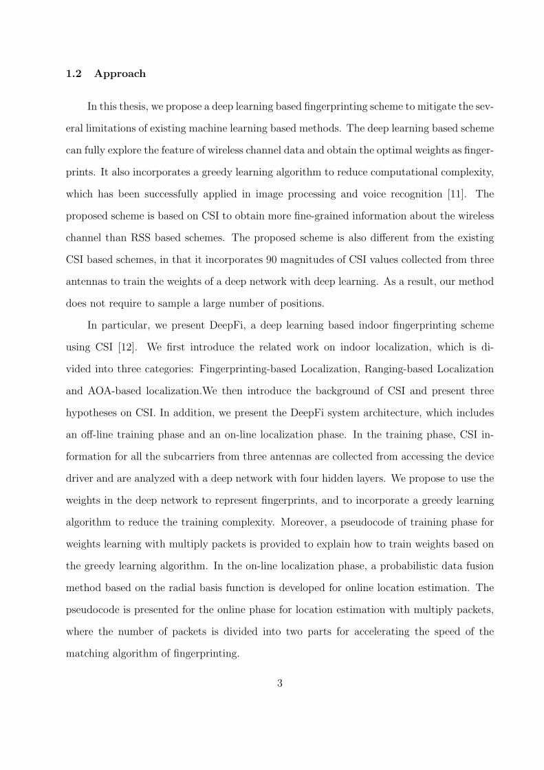
1.2 Approach

In this thesis, we propose a deep learning based fingerprinting scheme to mitigate the sev-

eral limitations of existing machine learning based methods. The deep learning based scheme

can fully explore the feature of wireless channel data and obtain the optimal weights as finger-

prints. It also incorporates a greedy learning algorithm to reduce computational complexity,

which has been successfully applied in image processing and voice recognition [11]. The

proposed scheme is based on CSI to obtain more fine-grained information about the wireless

channel than RSS based schemes. The proposed scheme is also different from the existing

CSI based schemes, in that it incorporates 90 magnitudes of CSI values collected from three

antennas to train the weights of a deep network with deep learning. As a result, our method

does not require to sample a large number of positions.

In particular, we present DeepFi, a deep learning based indoor fingerprinting scheme

using CSI [12]. We first introduce the related work on indoor localization, which is di-

vided into three categories: Fingerprinting-based Localization, Ranging-based Localization

and AOA-based localization.We then introduce the background of CSI and present three

hypotheses on CSI. In addition, we present the DeepFi system architecture, which includes

an off-line training phase and an on-line localization phase. In the training phase, CSI in-

formation for all the subcarriers from three antennas are collected from accessing the device

driver and are analyzed with a deep network with four hidden layers. We propose to use the

weights in the deep network to represent fingerprints, and to incorporate a greedy learning

algorithm to reduce the training complexity. Moreover, a pseudocode of training phase for

weights learning with multiply packets is provided to explain how to train weights based on

the greedy learning algorithm. In the on-line localization phase, a probabilistic data fusion

method based on the radial basis function is developed for online location estimation. The

pseudocode is presented for the online phase for location estimation with multiply packets,

where the number of packets is divided into two parts for accelerating the speed of the

matching algorithm of fingerprinting.

3

The proposed DeepFi scheme is validated with extensive experiments in two repre-

sentative indoor environments, i.e., a living room environment and a computer laboratory

environment. DeepFi is shown to outperform several existing RSSI and CSI based schemes in

both experiments. We also examine the effect of different DeepFi parameters on localization

accuracy, the effect of different environments on CSI properties with replaced obstacles and

human mobility, and the effect of the size of spot on localization accuracy.

1.3 Layout

The remainder of this thesis is organized as follows. We review the background and

recently proposed indoor localization schemes in Chapter 2, where the related work are clas-

sified into three categories. The CSI hypotheses and testbed implementation are described

in Chapter 3. In Chapter 4, we present the proposed DeepFi system. Experimental results

are presented and analyzed in Chapter 5. Chapter 6 concludes this thesis with a discussion

of future work.

4

Chapter 2

Background

There has been a considerable literature on indoor localization [13]. Early indoor loca-

tion service systems include (i) Active Badge equipped mobiles with infrared transmitters

and buildings with several infrared receivers [14], (ii) the Bat system that has a matrix

of RF-ultrasound receivers deployed on the ceiling [15], and (iii) the Cricket system that

equipped buildings with combined RF/ultrasound beacons [16]. All of these schemes achieve

high localization accuracy due to the dedicated infrastructure. Recently, considerable ef-

forts are made on indoor localization systems based on new hardware, with low cost, and

high accuracy. These recent work mainly fall into three categories: Fingerprinting-based,

Ranging-based and AOA-based, which are discussed in this chapter.

2.1 Fingerprinting-based Localization

Fingerprinting-based Localization incorporates a training phase and a test phase to

identify the most matched fingerprint for location estimation [17, 18]. As can be seen in

Fig. 2.1, the offline training phase is focused on preliminary data collection and processing.

A good collection method should carefully select the training points: neither too few, which

reduces the localization accuracy, nor too many, which requires a larger amount of data

collecting work. Then the collected data along with their corresponding positions are sent

to the server, which will train the data before saving it in the training database. Since most

of the raw data without training is chaotic and redundant, it is not an optimal choice for

fingerprints to be saved in the training database. Therefore some localization algorithms

process the raw data and then save the fingerprints for the test phase.

5

P(1)

{x,y}

Fingerprinting

(1)

P(2)

{x,y}

Fingerprinting

(2)

P(3)

{x,y}

Fingerprinting

(3)

P(n)

{x,y}

Fingerprinting

(n)

Training

Database

Fingerprinting

online

Position

Algorithm{x,y}

Offline training

phase

Mobile User Mobile User Location

Online determination

phase

Figure 2.1: The fingerprinting based localization model.

In the online test phase, when the mobile user moves to an unknown place, the finger-

prints corresponding to the current position are sent to the server for localization. Since

the database reserves already known the fingerprints and their corresponding positions, the

position algorithm can estimate the current position via seeking matched fingerprints in the

database. The location with the most matched fingerprints is most likely to be near the

current position. The server finds the optimal current position with a position algorithm,

and then sends the estimated location back to the mobile user.

Recently, there have been quite some efforts on developing various training algorithms.

Different fingerprints are proposed to improve localization accuracy, including WiFi [6], FM

radio [19], RFID [20], acoustic [21], GSM [22], light [23], and magnetism [24]. WiFi-based

fingerprinting is the dominant method because WiFi signal is ubiquitously accessible in

6

most indoor environments. The first work on WiFi fingerprinting is RADAR [3], which

builds fingerprints of RSSI using one or more access points with overlapped coverage of the

area of interest. Instead of raw data set of RSSI, processed data set including the standard

deviation and mean of the corresponding RSSI from each access point is acquired to describe

fingerprints. Therefore RADAR is considered as a deterministic method that uses the K-

nearest neighbor algorithm for position estimation.

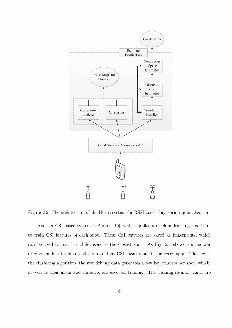
Another RSSI based scheme is Horus [6], which incorporates a probabilistic technique

to improve localization accuracy, where the RSSI of an AP is modeled as a random variable

over time and space. Fig. 2.2 shows the architecture of Horus, whose enhancements are

described as follows. Data collected from access points is first grouped in the clustering

module, which trains data in order to reduce computation in the test phase. Then the

correlation module calculates the average of a batch of correlated samples from collected

data in order to separate these points. In the online test phase, the Discrete Space Estimator

seeks the training point that has the maximum probability to match the realtime test data.

The Continuous Space Estimator take advantage of the continuity of human movement to

further improve localization accuracy.

In addition to using RSSI as fingerprints, channel impulse response of WiFi is considered

as a location-related and stable signature, which utilizes the signal characteristics of wireless

channel for localization. For example, FIFS [9] system exploits CSI information obtained

with the off-the-shelf Intel WiFi Link (IWL) 5300 Network Interface Card (NIC), which can

provide reliable fingerprints for location estimation. Fig. 2.3 shows the FIFS architecture,

which is the combination of two parts: the fingerprint generation block and the position

estimation block. The fingerprint generation block gathers CSI as fingerprints, which is

stored in the fingerprint database after some processing. Then when estimating position in

the online test phase, the localization server searches for the most matched position according

to the similarity between the stored and measured CSI values.

7

Signal Strength Acquisition API

ClusteringCorrelation

modeler

Radio Map and

Clusters

Correlation

Handler

Discrete-

Space

Estimator

Continuous

-Space

Estimator

Localization

Estimate

localization

Figure 2.2: The architecture of the Horus system for RSSI based fingerprinting localization.

Another CSI based system is PinLoc [10], which applies a machine learning algorithm

to train CSI features of each spot. These CSI features are saved as fingerprints, which

can be used to match mobile users to the closest spot. As Fig. 2.4 shows, during war

driving, mobile terminal collects abundant CSI measurements for every spot. Then with

the clustering algorithm, the war driving data generates a few key clusters per spot, which,

as well as their mean and variance, are used for training. The training results, which are

8

Fingerprints

Generation

Collect CSI

Process CSI

Position

Estimation

Positioning

Fingerprints

Mapping

Algorithm

Fingerprints

Database

Localization

Figure 2.3: The architecture of the FIFS system for CSI based fingerprinting localization.

War

Driving

Spot 1 Data

Spot 2 Data

Spot N Data

.

.

.

CFR

Clustering

Algorithm

Spot 1 Cluster 1

Spot 1 Cluster 2

.

.

.

Spot N Cluster 1

Spot N Cluster 2

Spot N Cluster 3

CFR

Classification

Test

Algorithm

Spot

Match

Online Data

Figure 2.4: The architecture of PinLoc system for fingerprinting localization with machinelearning.

reserved in the fingerprint database, are used to match online CSI measurements to estimate

position in the test phase. Although this technique achieves a high localization precision,

it requires large amounts of calibration to build the database via war driving, as well as

manually matching every spot with the corresponding fingerprints.

9

An alternative approach to reducing the burden of war driving is crowdsourcing, where

the fingerprints traced by multiple users are shared and used. The two major steps of crowd-

sourcing are (i) estimation of users trajectories and (ii) construction of the database mapped

from fingerprints to users locations [25], where trajectories of human movement are estimated

through crowdsourced data collected during user movement. Due to the relationship between

users trajectories and fingerprints, the fingerprints collected along with human movement

contribute to tracing users trajectories. Since crowdsourced data requires no prior known

conditions, there is no extra cost for users to trace their movement.

LiFS [26] is one of the crowdsourcing based localization schemes, which utilizes users

trajectories to obtain fingerprints and then builds the mapping between the fingerprints and

the floor plan. Another crowdsourcing scheme Zee [27] utilizes the inertial sensors and par-

ticle filtering to estimate users walking trajectory, and to collect fingerprints with WiFi data

as crowd-sourced measurements in the calibration step. Fig. 2.5 shows that there are mainly

two parts in the Zee system. In the first part is Placement Independent Motion Estimator,

where the motion estimator exploits the mixed data collected from accelerometer, compass

and gyroscope to estimate step counts and moving orientation. The other part combines

WiFi scanner, for collecting time-indexed WiFi information, and augmented particle filter,

which computes the joint probability distribution of users trajectories to perform localization.

On the other hand, one of the crowdsourcing applications is seeking indoor contexts

by constructing users traces. For example, CrowdInside [28] and Walkie-Markie [29] are

proposed to detect the floorplan and build the pathway to obtain the crowdsouced users

fingerprints. Fig. 2.6 shows the CrowdInside system architecture, which consists of three

parts, a data collection module, the motion trace generator, and the floorplan estimation

module. The data collection module gathers hybrid data along with human movement,

including accelerometer, gyroscope, RSSI of WiFi and GPS, which detects the transit from

outdoor to indoor. Then motion trace generator constructs precise user trajectories, which

has high accuracy because the trace is corrected by anchoring signature based on collected

10

Inertial Sensors

Accelerometer

Compass

Gyroscope

Motion Estimator

Step Counter

Heading Offset

Range

Estimation

WiFi Scanner

WiFi

Fingerprinting

Database

Augmented Particle

Filter

Floor Map

time-indexed

WiFi

information

Trajectories

Probability

DistributionLocalization

Figure 2.5: The architecture of zee system based on crowdsourcing localization.

hybrid data. At last the floorplan estimation module creates the building layout, which

distinguishes rooms, corridors, and block areas with the algorithm that flags the layout with

different classified traces and no trace pass areas.

In addition, Jigsaw [30] and Travi-Navi [31] combine the vision and mobility embedded

in smartphones to build user trajectory. Fig. 2.7 shows the three functional parts of Travi-

Navi. The motion engine block combines the Inertial Measurement Units (IMU) such as

accelerometer, gyroscope, and compass to implement step detection, rotation sense and

image capture. Then with WiFi, IMU and images from the previous block, the trace packing

block creates users traces that are reversed in server. The navigation engine block works in

the online phase when recommending route for users. Combined with users position that

is corrected by WiFi and IMU fingerprints, Travi-Navi provides suggested routes to the

destination based on detected shortcuts. Although crowdsourcing based localization does

not require large amounts of calibration, it obtains coarse grained fingerprints, which thus

leading to low localization accuracy.

11

Data Collection Module

Motion Traces Generator

Inertial Sensors

anchoring

signature

Trace

Segmentation

Segmentation

Classification

Shape & Labels

Assignment

Floorplan Estimation

Figure 2.6: The architecture of CrowdInside system for Estimating floorplan.

2.2 Ranging-based Localization

Instead of manually constructing fingerprints, ranging-based localization leverages geo-

metrical models to determine the location of a mobile user by computing distances to at least

three APs. Such schemes are mainly classified into two categories: power-based and time-

based. For power-based approaches, the prevalent log-distance path loss (LDPL) model [32]

is used to estimate the distances based on RSS, where some measurements are utilized to

train the parameters of LDPL model.

12

Motion Engine

Inertial Measurement Units (IMU)

Accelerometer & Compass & Gyroscope

Camera

WiFi Scanner

Step Dection

Image Capture

WiFi

Trace

Packing

Shortcuts

Detection

Navigation

Engine

Localization &

Routes

Instruction

Figure 2.7: The architecture of Travi-Navi system for navigation.

AP1 {X1, Y1}

AP2 {X2, Y2}

Ap3 {X3, Y3}

AP4 {X4, Y4}

AP5 {X5, Y5}

<RSSI, d>

<RSSI, d>

<RSSI, d>

<RSSI, d><RSSI, d>

Figure 2.8: The ranging based localization model.

As show in Fig. 2.8, a simplified power-based localization system deploys APs with

known positions and overlapped coverages. The APs broadcast beacons to their nearby

mobile users who collect RSSI from the APs within range. Due to the assumption that

the path loss when signal propagates in the indoor environment follows the LDPL model,

the distance between an AP and the mobile terminal can be estimated using the RSSI.

When served by three or more APs, the mobile user collects RSSI from three links, which

13

provide three relative distances from the user to the APs. With known positions of APs

and corresponding relative distances, the users position can be estimated with geometric

computations [33].

The LDPL model can be written as

PL = PL(d0) + 10α log

(

d

d0

)

, (2.1)

where PL is the path loss measured in dB and PL(d0) is pass loss at reference distance d,

which is 1 m in the indoor environment; α is the path loss exponent, which is set to 2.6

experimentally.

Increasing attention is attracted on ranging-based localization for its desirable advantage

of easy deployment. Unlike fingerprinting based localization, ranging-based localization has

no requirement for pre-process of fingerprinting, which usually requires enormous work. For

example, EZ [34] is a configuration-free localization scheme without any pre-deployment

effort, which utilizes a genetic algorithm for solving RSS-distance equations to locate mobile

devices.

Due to the effects of multipath fading and shadowing in indoor environments, the path

loss usually does not strictly follow LDPL but requires more consideration of dynamic chan-

nel frequency response. Lim et al. use the LDPL model and the truncated singular value

decomposition (SVD) model to build an RSS-distance map for localization, which is respon-

sive to indoor environmental dynamics [32]

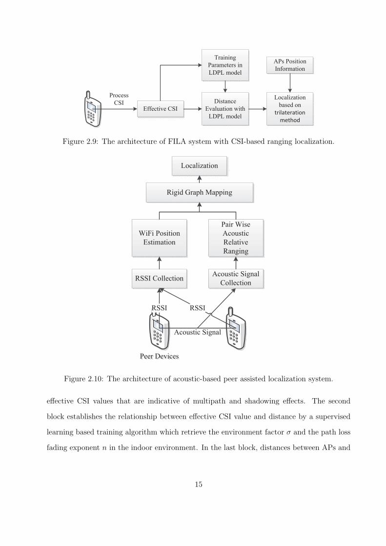
To avoid the instability of RSS due to indoor multipath propagation, CSI-based ranging

is used to improve indoor localization accuracy. For instance, FILA exploits CSI from the

PHY Layer to mitigate the multipath effect in the time domain, and then trains the pa-

rameters of LDPL model to obtain the relationship between the effective CSI and distance,

thus leading to an accurate localization system [35]. FILA consists of three main blocks,

as shown in Fig. 2.9. The first block deals with CSI processing, which as a result produces

14

Effective CSI

Process

CSI

Training

Parameters in

LDPL model

Distance

Evaluation with

LDPL model

Localization

based on

trilateration

method

APs Position

Information

Figure 2.9: The architecture of FILA system with CSI-based ranging localization.

Peer Devices

RSSI CollectionAcoustic Signal

Collection

RSSI RSSI

Acoustic Signal

WiFi Position

Estimation

Pair Wise

Acoustic

Relative

Ranging

Rigid Graph Mapping

Localization

Figure 2.10: The architecture of acoustic-based peer assisted localization system.

effective CSI values that are indicative of multipath and shadowing effects. The second

block establishes the relationship between effective CSI value and distance by a supervised

learning based training algorithm which retrieve the environment factor σ and the path loss

fading exponent n in the indoor environment. In the last block, distances between APs and

15

the user are estimated based on the refined propagation model, and then the mobile user’s

location is obtained via trilateration.

On the other hand, acoustic-based ranging approaches are designed for improving in-

door localization precision. H. Liu et al. propose a peer assisted localization technique based

on smartphones to get accurate distance estimation among peer smartphones from acoustic

ranging [36]. As shown in Fig. 2.10, the peer assisted localization requires two samples, one

is RSSI based on WiFi, which is used to estimate a coarse user location, and the other is

acoustic signal from the peer stations which is used to estimate the precise relative distance.

Then combining distances estimated from both RSSI and acoustic, a mapping algorithm

searches for the optimal position of user by minimizing the sum of RSS Euclidean distances,

which mitigates the error as two faraway points usually do not share a similar WiFi sig-

nal. a In addition, Centour [37] leverages a Bayesian framework to jointly exploit WiFi

measurements and acoustic ranging for localization, where two new acoustic techniques are

proposed for ranging in NLOS and locating a speaker-only device based on estimating dis-

tance differences. Guoguo [38] is an indoor localization system based on smartphone, which

estimates a fine-grained time-of-arrival (TOA) by using beacon signals and implementing

NLOS identification.

2.3 AOA-based Localization

Indoor localization based on angle-of-arrival (AOA) utilizes multiple antennas to esti-

mate the incoming angles and then uses geometric relationships to obtain the location of the

mobile user. This technique is not only with zero start-up cost (i.e., it does not require rich

fingerprinting by training or crowdsourcing), but also with higher accuracy than other tech-

niques such as RF fingerprinting or ranging-based systems. Fig. 2.11 illustrates the simplest

angle-of-arrival estimation algorithm, which utilizes the difference in the phases of arriving

signals to compute the corresponding differential length in form of wavelength. It then esti-

mates the arrival angle based on a geometrical methodology. However, since the real wireless

16

Incoming Signal

Wavelength

Disfference

Half of

Wavelength

Angle of

Incidence

Figure 2.11: The Angle-of-Arrival Algorithm presented in wireless router with two antennas.

−90 −60 −30 0 30 60 90−20

−15

−10

−5

0

Angle (degree)

Mag

nit

ud

e (d

B)

Angle of Direct Path

Figure 2.12: Direct path estimation with the MUSIC algorithm.

signal is affected by multiple paths, a practical angle-of-arrival estimation algorithm, called

MUSIC [39], can be used to distinguish multiple arrival angles. Fig. 2.12 shows an example

result of MUSIC, where each peak corresponds to the arrival angle of each of the multiple

paths. Since the direct path has the strongest energy if LOS is available, the highest peak

indicates the angle of the direct path.

17

a b

ab

Change

of angle

Figure 2.13: Illustration to refine location in CUPID with AOA-based localization.

The challenge of the MUSIC algorithm is how to improve the resolution of the antenna

array. The recently proposed CUPID system [40] uses off-the-shelf Atheros chipsets with

three antennas to obtain CSI for AOA estimation. It can achieve a mean error about 20

degree based on MUSIC. The main idea of CUPID is shown in Fig. 2.13. When the user

moves from position A to B, the three sides of the triangle are measured. Specifically, Da

and Db are estimated by their corresponding signal strength with a path loss model and Pab

is estimated by the IMU with the dead reckoning method. Since the change of angle of the

direct path, which is computed from Da, Db and Pab, cause elimination of the interfering

angles estimated by MUSIC, the user position is finally computed via refining its distance

and the real direct path. However, the main disadvantage of CUPID, which leads to its poor

localization performance with MUSIC, is the low resolution of the antennas array, which

contains only three antennas with the Atheros 9390 chipset.

For obtaining high localization accuracy, the ArrayTrack system [41] implemented with

two WARP FPGA-based software defined radios (SDR) utilizes a rectangular array of 16

antennas to compute the AOA, and then uses spatial smoothing to suppress the effect of

multipath on AOA. Fig. 2.14 shows the architecture of ArrayTrack that consists of two parts,

the AP and the ArrayTrack server. The AP is able to detect packets even with low density

18

Access Point

Diversity Synthesis Algorithm

ArrayTrack Server

AOA Spectrum Generation

Multipath Suppression Algorithm

Maximum Likelihood Estimation for

Localization

Figure 2.14: The architecture of the Arraytrack system implemented on antenna array.

and power signal due to the diversity synthesis algorithm, which enables quick switches be-

tween antenna pairs to enhance received signal strength. On the other hand, the ArrayTrack

server gathers AOA data from multiple antennas, which generates an accurate spectrum to

indicate signal power. Since the direct path is usually overwhelmed by multipath reflec-

tions, the spectrum is further refined by a multipath suppression algorithm by mitigating

the multipath effect without changes on the direct path. Finally ArrayTrack employs maxi-

mum likelihood estimation for localization estimation through combining information from

several near APs each with a likelihood probability associated with the spectrum. However,

this ArrayTrack system requires a large number of antennas (such as 16 antennas), which is

impractical to apply with commodity mobile devices.

On the other hand, some systems, such as LTEye [42], Ubicarse [43], Wi-Vi [44], and

PinIt [45], use Synthetic Aperture Radar (SAR) to mimic an antenna array to improve the

resolution of angles. In other words, the main idea of SAR is to use a moving antenna to

obtain signal snapshots as it moves along its trajectory, and then to utilize these snapshots

19

r Y

Z

X

Antenna

Rotation

Direction

Signal

Direction

Take a Snapshot

Figure 2.15: The circular SAR with rotating antenna.

to mimic a large antenna array with this trajectory. Fig. 2.15 illustrates a circular SAR,

which emulates a circular antenna array as the antenna rotates round a circle. Since both the

snapshots captured at the gray points in the circle trajectory and their accurate positions are

measured in SAR, SAR is able to apply antenna array equations to solve for the multipath

profile. However, the existing limitation of SAR is that it requires extremely precise control

of the speed and its trajectory by employing a moving antenna placed on an iRobot Create

robot.

20

Chapter 3

Hypotheses and Testbed Implementation

3.1 Channel State Information

Thanks to the advanced NICs, such as Intel’s IWL 5300, it is now easier to conduct

channel state measurements than in the recent past when one has to detect hardware records

for physical layer (PHY) information. Now CSI can be retrieved from a laptop by accessing

the device drive. CSI records the channel variation experienced during propagation. Trans-

mitted from a source, a wireless signal may experience abundant impairments caused by,

e.g., the multipath effect, fading, shadowing, and delay distortion. Without CSI, it is hard

to reveal the channel characteristics with only the signal power.

Let ~X and ~Y denote the transmitted and received signal vectors. We have

~Y = CSI · ~X + ~N, (3.1)

where vector ~N is the additive white Gaussian noise and CSI represents the channel’s fre-

quency response, which can be estimated from ~X and ~Y .

The WiFi channel at the 2.4 GHz band can be considered as a narrowband flat fading

channel. The Intel WiFi Link 5300 NIC implements an OFDM system with 48 subcarriers,

30 out of which can be read for CSI information via the device driver. The channel frequency

response CSIi of subcarrier i is a complex value, which is defined by

CSIi = |CSIi| exp {j(∠CSIi)}. (3.2)

21

where |CSIi| and ∠CSIi are the amplitude response and the phase response of subcarrier i,

respectively. In this thesis, the proposed DeepFi framework is based on these 30 subcarriers

(or, CSI values) in the OFDM system, which can reveal completely different properties than

RSSI.

3.2 Hypotheses

We next present three hypotheses about the CSI data, which are validated with the

statistical results through our measurement study.

3.2.1 Hypotheses 1

CSI values are stable at a fixed location but exhibit large variability at adjacent locations.

CSI values reflect channel properties in the frequency domain and exhibit great stability

over time for the same location. Fig. 3.1 plots the CDF of the standard deviations of

normalized CSI and RSS amplitudes for 150 sampled locations. At each location, CSI and

RSS are measured from 50 received packets with the three antennas of Intel WiFi Link 5300

NIC. It can be seen that for CSI, 90% of the standard deviations are blow 10% of the average

value; for RSS, however, 60% of the standard deviations are blow 10% of the average value.

Therefore CSI is much more stable than RSSI. The stability of CSI values is also invariant to

changes in the indoor environment. Our measurements last a long period covering both office

hours and quiet hours. No obvious difference in the stability of CSI for the same location is

found at different times. On the contrary, RSS values usually vary greatly even at the same

position.

On the other hand, another characteristic of CSI is the apparent variability at different

locations. Fig. 3.2 plots the subcarrier amplitudes for 50 back-to-back packet receptions

from three adjacent positions, from which hardly any similar trend can be observed.

22

0 0.2 0.4 0.6 0.8 10

0.1

0.2

0.3

0.4

0.5

0.6

0.7

0.8

0.9

1

Std of Normalized Amplitude of CSI

CD

F

CSIRSS

Figure 3.1: CDF of the standard deviation of CSI and RSS amplitudes for 150 sampledlocations.

0 5 10 15 20 25 300

5

10

15

20

25

30

35

40

Subcarrier (f)

Am

pli

tude (

dB

)

Figure 3.2: Amplitudes of channel frequency responses of 50 packets measured at threedifferent locations.

23

1 2 3 4 5 60

0.2

0.4

0.6

0.8

1

The Number of CSI Clusters

CD

F

Figure 3.3: CDF of the number of channel frequency responses at 50 different locations.

0 5 10 15 20 25 300

5

10

15

20

25

30

35

40

Subcarrier (f)

Am

pli

tude (

dB

)

Figure 3.4: Amplitudes of channel frequency response measured at the three antennas of theIntel WiFi Link 5300 NIC (each is plotted in a different color) for 50 received packets.

24

3.2.2 Hypotheses 2

The multipath effect causes clusters of CSI values from the subcarriers with respect to

the attenuation experienced by the subcarriers.

CSI values reflect channel frequency responses with abundant multipath components

and channel fading. The indoor environment can be viewed as a time-varying channel, and

therefore CSI may change slightly over time. Our study of channel frequency responses show

that there are several dominant clusters of subcarriers for a fixed location, while each cluster

consists of a subset of subcarriers with similar CSI values. Fig. 3.3 presents the distribution

of number of clusters for 50 different locations. As shown in Fig. 3.3, most of the locations

have two or three clusters. We also find that some locations has only one cluster, which

usually means that there is less reflection and diffusion. Some other locations with five or

six clusters may suffer more from the multipath effect.

To detect all possible numbers of clusters, we measure CSI from received packets for

a long period of time at each location. Since a lot of data are needed to train the specific

characteristics in deep learning, more packet transmissions will be helpful to reveal the

comprehensive properties at each spot. In our experiments, 1000 packets are recorded for

training at each location, more than the 60 packets used in FIFS.

3.2.3 Hypotheses 3

The three antennas of the Intel WiFi Link 5300 NIC have different CSI features, which

can be exploited to improve the diversity of training samples.

Intel WiFi Link 5300 is equipped with three antennas. We find that the channel fre-

quency responses of the three antennas are highly different, even for the same packet re-

ception. In Fig. 3.4, signals from the three antennas exhibit very different properties. In

FIFS, CSI from the three antennas are simply accumulated to produce an average value.

In contrast, DeepFi aims to utilize their variability to enhance the training process in deep

learning. The 30 subcarriers can be treated as 30 nodes and used as input data of visible

25

variability for deep learning training. With the three antennas, there are 90 nodes that can

be used as input data for deep learning training. The greatly increased number of nodes for

input data can improve the diversity of training samples, leading to better performance of

localization if reasonable parameters are chosen.

3.3 Experiment Setup

3.3.1 Hardware Implementation

In our experiments, we employ Intel WiFi Link 5300 network interface card (NIC) as

wireless receiver to record channel frequency response (CFR). Unlike other NICs which can

only obtain CFR in the form of RSSI, IWL 5300, which supports the 802.11n standard, allows

us to record channel state information (CSI) between the transmitter and receiver. Equipped

with three antennas, IWL 5300 is able to offer signal strengths and phases of the subcarriers

of a practical OFDM system. The CSI consists of 30 readable groups of subcarriers, each

group is an OFDM subcarrier containing two orthogonal signals in complex form. There

are two operation modes with different bandwidth for IWL 5300. One mode uses 20MHz

channels with 56 groups of subcarriers and the other mode uses 40MHz channels with 114

groups of subcarriers. The 30 readable groups are evenly distributed within these 56 or 114

groups in either modes.

Fig. 3.6 illustrates the platform of IWL 5300, a portable mini NIC with a 2.5 inch size.

In our system, the IWL 5300 is installed in a Dell laptop as shown in Fig. 3.5, which runs a

32-bit Ubuntu Linux Operating System (OS), version 10.04LTS of the Server Edition. This

Linux version has the 2.6.36 kernel, which is then modified by us in order to access to the

CSI records from the NIC. The modified kernel is derived from a released modified firmware,

which is based on Intels close-source firmware and open-source iwlwifi wireless driver. Thanks

to the modified firmware, we can now access the Intel debug mode in which CSI values are

obtained and saved in the laptop. For each received packet, there is an integrated CSI data

26

CSI Process

[ ]1 2 90| | | CSI | | CSI | | CSI |=CSI

Location 1

Data

Deep Learning

Location 2

Data

Location N

Data

Location 2

Weights

Location N

Weights

Location1

Weights

Data FusionTest Location X

Data

Estimated Location

Access PointMobile DeviceSuccessive Packets

Normalization

Online

Offline

Figure 3.5: The DeepFi Architecture.

saved in a file, which will be used for data analysis at the host server when all packets have

been received.

3.3.2 System Configuration and Development

Since IWL 5300 has a limitation on the Intels close-source firmware, we cannot directly

access to the NIC memory for CSI. However, thanks to an open-source iwlwifi wireless

driver, we can enable the debug mode of IWL 5300, which allows the NIC to report CSI to

the main memory. Therefore, we install a new kernel based on the modified iwlwifi driver

on the Linux server OS. Running with the new kernel, the Ubuntu is able to report CSI

through a C program and export CSI as a file. In the next step, the files of saved CSI are

27

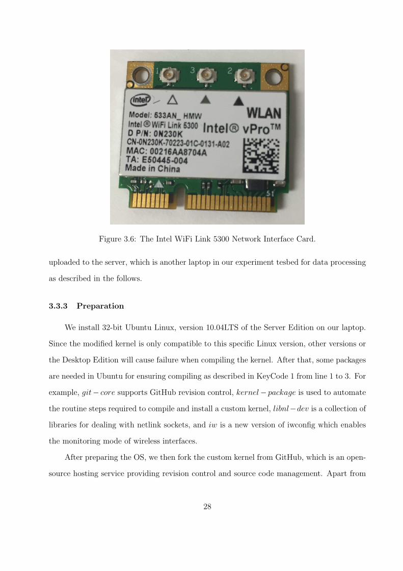
Figure 3.6: The Intel WiFi Link 5300 Network Interface Card.

uploaded to the server, which is another laptop in our experiment tesbed for data processing

as described in the follows.

3.3.3 Preparation

We install 32-bit Ubuntu Linux, version 10.04LTS of the Server Edition on our laptop.

Since the modified kernel is only compatible to this specific Linux version, other versions or

the Desktop Edition will cause failure when compiling the kernel. After that, some packages

are needed in Ubuntu for ensuring compiling as described in KeyCode 1 from line 1 to 3. For

example, git− core supports GitHub revision control, kernel− package is used to automate

the routine steps required to compile and install a custom kernel, libnl−dev is a collection of

libraries for dealing with netlink sockets, and iw is a new version of iwconfig which enables

the monitoring mode of wireless interfaces.

After preparing the OS, we then fork the custom kernel from GitHub, which is an open-

source hosting service providing revision control and source code management. Apart from

28

KeyCode 1: Prepare to Compile the Kernel

1 //install necessary packages;2 sudo apt-get -y install git-core kernel-package fakeroot build-essential ncurses-dev;3 sudo apt-get -y install libnl-dev libssl-dev;4 sudo apt-get -y install iw;5 //fork code from GitHub;6 git clone -b csitool-stable git://github.com/mars920314/linux-80211n-csitool.git;7 git clone git://github.com/mars920314/linux-80211n-csitool-supplementary.git;8 git clone git://github.com/mars920314/hostap-07.git;

the custom kernel, some supplementary files including configuration tools and data reading

scripts are also appended together. We download the latest branch from our account in

Git (https://git-scm.com/) as shown in KeyCode 1 from line 4 to 6. Three branches are

needed. The linux−80211n−csitool includes custom kernel. The linux−80211n−csitool−

supplementary includes custom firmware of iwlwifi. The hostap−07 is one of IEEE802.11

device driver for Linux, which enables a WLAN card to execute all functions of a wireless

AP and 07 stands for a stable version.

3.3.4 Installation

In this step, we first configure the kernel before compile it. Since an optimized kernel

configuration is recommended in the branch, we can directly utilize it instead of the Ubuntu

default configuration under the root path. We change the current directory to linux −

80211n − csitool, the file we have downloaded in the previous step, where the customized

configuration, named .config, is included. We then build the process and choose the feature

of kernel as described in KeyCode 2 (lines 2 and 3). After a long time of compiling, the next

step is to install the customized kernel (line 4 and 5). Then we create a boot option, whose

name is tagged by CSI, and update GRUB, which provides boot management (line 6 and 7).

Second, we install the Linux kernel−headers, which is needed for reading CSI from IWL

5300. We then copy linux− headers at usr/include/ to the root directory, ./usr/include/,

29

KeyCode 2: Install the Kernel

1 //configure and compile the custom kernel;2 cd linux-80211n-csitool;3 make oldconfig;4 make menuconfig;5 //install the kernel;6 make -j3 bzImage modules;7 sudo make install modules install;8 //update GRUB;9 sudo mkinitramfs -o /boot/initrd.img-‘cat include/config/kernel.release‘ ‘catinclude/config/kernel.release‘;

10 sudo update-grub;

KeyCode 3: Install the Linux Kernel-headers

1 //install the Linux kernel-headers;2 make headers install;3 sudo mkdir /usr/src/linux-headers-‘cat include/config/kernel.release‘;4 sudo cp -rf usr/include /usr/src/linux-headers-‘catinclude/config/kernel.release‘/include;

as described in KeyCode 3 (line 2 and 3). After installation, reboot the Ubuntu and choose

the new kernel, whose name is CSI in our laptop.

Third, we have to install the custom firmware which is under the directory linux −

80211n − csitool − supplementary/firmware/. We replace the original firmware named

iwlwifi−5000−2.ucode with the custom firmware named iwlwifi−5000−2.ucode.sigcomm2010

as described in KeyCode 4 (line 2). Considering for future reference, we backup the orig-

inal firmware in advance. Then we compile hostapd, which enables the Host AP mode

for IWL 5300. Since the custom configuration file for compiling hostapd is at linux −

80211n − csitool − supplementary/hostap − config − files/, we copy this configuration

file, named hostap− dotconfig, to the compiling dictionary, hostap− 07/hostapd, and then

compile (line 3 to 5) it. The last step is to compile the tool that logs CSI in directory

linux− 80211n− csitool − supplementary/netlink (line 6 and 7).

30

KeyCode 4: Install the Custom Firmware

1 //install the custom firmware;2 sudo cp /lib/firmware/iwlwifi-5000-2.ucode /lib/firmware/iwlwifi-5000-2.ucode.orig;3 sudo cp iwlwifi-5000-2.ucode.sigcomm2010 /lib/firmware/iwlwifi-5000-2.ucode;4 //compile hostapd;5 cd hostap-07/hostapd;6 cp linux-80211n-csitool-supplementary/hostap-config-files/hostap-dotconfig .config;7 make;8 //compile reading CSI tool;9 cd linux-80211n-csitool-supplementary/netlink;

10 make;

3.3.5 Execution

With the above steps, we have completed installing the required platform for CSI col-

lection. In the next step, we report CSI from the IWL 5300 cards between the laptop and

wireless router.

Before logging CSI, the laptop equipped with IWL 5300 needs to connect to the AP,

i.e., the TP Link wireless router. There are some limitations for setting up the router. First,

since CSI is based on the IEEE 802.11n standard, the wireless mode of router is configured to

support IEEE 802.11n. Second, because we prefer to utilize the 20MHz channel bandwidth

mode of IWL 5300, the channel bandwidth of the router should also be configured to 20MHz.

Third, since the custom firmware has limited bits for code, there is no enough bits for both the

beamforming software path, which is required to measure CSI, and the encryption software

paths, which is required for WEP/NWPA/WPA2/etc. functions. We configure the router

without encryption with security-free connections. The AP’s SSID is set to Auburn314 and

its IP address is 192.168.0.1.

First, the Ubuntu server associates to the router using the bash command. Since we

have modified the NIC driver, we have to prevent some modules from being automatically

loaded by removing these modules, including iwlwifi, mac80211, and cfg80211. We then

reload the custom module iwlwifi that supports CSI reports as described in KeyCode 5

(line 1 and 2). Since IWL 5300 is denoted as wlan1, we configure wlan1 to connect the AP

31

KeyCode 5: Connect to Wireless Router

1 //remove and reload modules;2 sudo rmmod iwlwifi mac80211 cfg80211;3 sudo modprobe iwlwifi connector log=0x01;4 //connect to wireless router;5 Sudo iwconfig wlan1 essid Auburn314;6 Sudo dhclient wlan1;

named Auburn314. We then request the server to automatically assign an IP address to

wlan1 (line 3 and 4).

After connecting to the router, two different terminals are required for logging CSI. One

terminal runs the program that is used to report CSI, the other terminal continuously Pings

the IP address of router. In the first terminal tty1, since the program for logging CSI has

been compiled in folder linux − 80211n − csitool − supplementary/netlink, we run the C

code named log to file and consequently export the CSI file as described in KeyCode 6 (line

1 and 2).

In the second terminal tty2, since the laptop needs to receive packets from the router,

we utilize the Ping command to build sessions between the laptop and router. Each time

the laptop receives a response from the router, the program log to file in tty1 will process

the received packet as well as logging CSI. Since only one CSI data is recorded for each

received packet, we need to continuously receive multiple packets, to collect enough CSI

values for training and location estimation. For example, 1000 packets are collected for each

training point and 100 packets are collected for each test point. In order to achieve successive

collection, we execute a customized Java program to replace the bash command (line 3). The

Java program creates a thread every 50 ms, each thread executes one command, which Pings

the IP address of the router, i.e., 192.168.0.1/24. After recursive Pings, the CSI recorded

from all the packets will be written into a file, which can be read by a customized script for

processing.

32

KeyCode 6: Log CSI

1 //log CSI in tty1;2 cd linux-80211n-csitool-supplementary/netlink;3 sudo ./log to file CSIfile;4 //Ping the IP address of router in tty2;5 Java jar pingjava.jar 192.168.0.1 1000;

3.4 Data Processing

3.4.1 Data format

After collecting the CSI data, we export the measured CSI reports from the mobile

device to the server for processing. The server here is a PC that runs MATLAB to process

the CSI data. First, since the original CSI report is in the format of binary files, we utilize

the mex compiled C program in MATLAB to read the binary CSI data. The unpacked

format of processing result is n structs compacted in a cell. There are n correctly received

CSI packets corresponding to the equal n structs, each of which contains antenna parameters

as well as raw CSI values. Then these parameters are utilized to calculate normalized CSI

values, which are needed via corrected raw CSI values.

In each correctly received packet, not only the CSI value but also antenna parameters

for receiving the packet are saved in the report. The data format is described below.

• T imestamp low is the low 32 bits of the 1 MHz clock in NIC.

• Bfee count counts the number of packet received by the driver. If a packet is lost

between the kernel and user space, Bfee count can detect this error.

• Nrx is the amount of occupied antennas when receiving packets, while Ntx is the

amount of antennas used to transmit packets.

• Rssi is received signal strength indication of input receiving signal whose value is in

format of dB. The suffix a, b and c stand for the values of corresponding antenna a,

33

b and c. In addition, the received signal strength is got by adjusting this value by

automatic gain control value and a constant magnification factor.

• Noise is the thermal noise measured during reception in dB. There is a fact that the

thermal noise might be undefined when NIC works in the monitor mode. Therefore, if

the noise value is -127, which is an initial value without modification, it is replaced by

a hard coding noise floor value, which is -92 as recommended.

• AGC stands for automatic gain control value in dB.

• Perm presents the order of three receive antenna.

• Rate is the transmission bit rate including all occupied antennas. Bit rate can be

modified as needed.

• CSI is the raw CSI values relative to a NIC internal reference. It is a three dimension

matrix of Ntx × Nrx × 30, in which the third dimension with 30 values stand for 30

OFDM subcarriers.

3.4.2 CSI Figure

Instead of raw CSI values in packets, the normalized CSI values represent the actually

received signal by removing the NIC internal reference. We process raw CSI value in MAT-

LAB by dividing it with a noise factor. The noise factor is derived from two parts, one is the

thermal noise, and the other is the quantization error which is divided by Nrx ×Ntx entries.

We then divide the raw CSI by the noise factor to get unit of squared SNR, which is the

normalized CSI value we need.

Fig. 3.7 plots the normalized CSI from three antennas for one received packet. Due to

the complex form signals in OFDM, we calculate the amplitude of each subcarrier. In this

figure, the green line above the rest two lines stands for the CSI of antenna C, which has

the largest RSSI of 44 dB. The rest two antennas has relatively lower RSSI, i.e., 38 dB for

34

5 10 15 20 25 3020

21

22

23

24

25

26

27

28

29

30

Subcarrier Index

SN

R [d

B]

antenna Aantenna Bantenna C

Figure 3.7: The CSI from the three antennas collected from one received packet.

antenna A and 37 dB for antenna B. Since this packet is received in an empty space, its

CSI represent a typical case of LOS reception, in which, as we expect, there is no significant

frequency selective fading observed.

35

Chapter 4

The DeepFi System

4.1 System Architecture

Fig. 3.5 shows the system architecture of DeepFi, which only requires one access point

and one mobile device equipped with an Intel WiFi link 5300 NIC. At the mobile device, raw

CSI values can be read from the modified chipset firmware for received packets. The Intel

WiFi link 5300 NIC has three antennas, each of which can collect CSI data from 30 different

subcarriers. We can thus obtain 90 raw CSI values for each packet reception. Unlike FIFS

that averages over multiple antennas to reduce the received noise, our system uses all CSI

values from the three antennas for indoor fingerprint to exploit diversity of the multiple-

input and multiple-output (MIMO) channel. Since it is hard to use the phases of CSI values

for localization, we only consider the amplitude responses for fingerprinting. On the other

hand, since the input values should be limited in the range (0, 1) for effective deep learning,

we normalize the amplitudes of the 90 CSI values for both the offline and online phases.

In the offline training phase, DeepFi generates feature-based fingerprints, which are

greatly different from the traditional methods that are based on clustering. Feature-based

fingerprints utilize a large number of weights obtained by deep learning to denote different

locations, which effectively describe the characteristics of CSI values for each location. The

feature-based fingerprints server can store the weights for different training locations. In the

online localization phase, the mobile device can estimate its position based on data fusion,

which normalizes the magnitudes of CSI values using weights from different positions to

obtain its estimated location.

36

Neurons

| |CSIuuuuuuv

Normalization

Neurons

Neurons

Neurons

R

| |CSIuuuuuuv

Reconstruction

Neurons

Neurons

Neurons

1W

2W

3W

4W

4

TW

3

TW

2

TW

1

TW

∑

−+ Error

Pretraining

Unrolling

Fine-tuning

Successive Packets

1K

2K

3K

4K

3K

2K

1K

Figure 4.1: Weight training with deep learning.

4.2 Weight Training with Deep Learning

Fig. 4.1 illustrates how to train weights based on deep learning. There are three stages

in the procedure, including pre-training, unrolling, and fine-tuning [46]. In the pre-training

stage, it is a deep network with four hidden layers, where every hidden layer consists of a

different number of neurons. In order to reduce the dimension of CSI data, we assume that

37

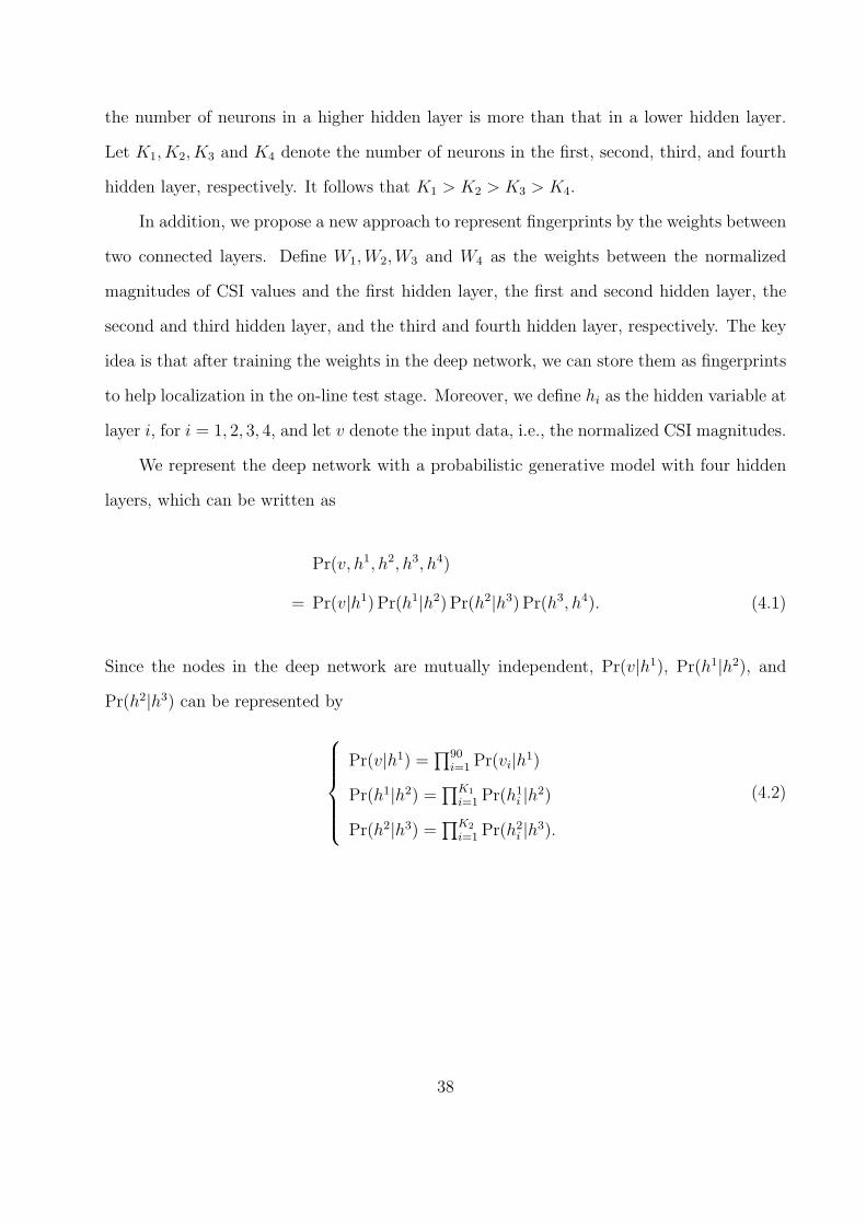
the number of neurons in a higher hidden layer is more than that in a lower hidden layer.

Let K1, K2, K3 and K4 denote the number of neurons in the first, second, third, and fourth

hidden layer, respectively. It follows that K1 > K2 > K3 > K4.

In addition, we propose a new approach to represent fingerprints by the weights between

two connected layers. Define W1,W2,W3 and W4 as the weights between the normalized

magnitudes of CSI values and the first hidden layer, the first and second hidden layer, the

second and third hidden layer, and the third and fourth hidden layer, respectively. The key

idea is that after training the weights in the deep network, we can store them as fingerprints

to help localization in the on-line test stage. Moreover, we define hi as the hidden variable at

layer i, for i = 1, 2, 3, 4, and let v denote the input data, i.e., the normalized CSI magnitudes.

We represent the deep network with a probabilistic generative model with four hidden

layers, which can be written as

Pr(v, h1, h2, h3, h4)

= Pr(v|h1) Pr(h1|h2) Pr(h2|h3) Pr(h3, h4). (4.1)

Since the nodes in the deep network are mutually independent, Pr(v|h1), Pr(h1|h2), and

Pr(h2|h3) can be represented by

Pr(v|h1) =∏

90

i=1Pr(vi|h1)

Pr(h1|h2) =∏K1

i=1Pr(h1

i |h2)

Pr(h2|h3) =∏K2

i=1Pr(h2

i |h3).

(4.2)

38

In (4.2), Pr(vi|h1), Pr(h1

i |h2), and Pr(h2

i |h3) are described by the sigmoid belief network in

the deep network, as

Pr(vi|h1) = 1/(

1 + exp (−b0i −∑K1

j=1W i,j

1h1

j))

Pr(h1

i |h2) = 1/(

1 + exp (−b1i −∑K2

j=1W i,j

2h2

j))

Pr(h2

i |h3) = 1/(

1 + exp (−b2i −∑K3

j=1W i,j

3h3

j))

,

(4.3)

where b0i , b1

i and b2i are the biases for unit i of input data v, unit i of layer 1, and unit i of

layer 2, respectively. On the other hand, the joint distribution Pr(h3, h4) can be expressed as

an Restricted Boltzmann Machine (RBM) with a bipartite undirected graphical model [47],

which is given by

Pr(h3, h4) =1

Zexp(−E(h3, h4)), (4.4)

where

Z =∑

h3

∑

h4

exp(−E(h3, h4)) (4.5)

E(h3, h4) = −K3∑

i=1

b3ih3

i −K4∑

j=1

b4jh3

j −K3∑

i=1

K4∑

j=1

W i,j4h3

ih4

j . (4.6)

In fact, since it is difficult to find the joint distribution Pr(h3, h4), we use the contrastive

divergence (CD) algorithm to approximate it, which is given by

Pr(h3|h4) =∏K3

i=1Pr(h3

i |h4)

Pr(h4|h3) =∏K4

i=1Pr(h4

i |h3),(4.7)

39

where Pr(h3

i |h4), and Pr(h4

i |h3) are described by the sigmoid belief network, as

Pr(h3

i |h4) = 1/(

1 + exp (−b3i −∑K4

j=1W i,j

4h4

j))

Pr(h4

i |h3) = 1/(

1 + exp (−b4i −∑K3

j=1W i,j

4h3

j))

.(4.8)

Finally, the marginal distribution of input data for the deep belief network is given by

Pr(v) =∑

h1

∑

h2

∑

h3

∑

h4

Pr(v, h1, h2, h3, h4). (4.9)

Due to the complex model structure with the large number of neurons and multiple

hidden layers in the deep belief network, it is difficult to obtain the weights using the given

input data with the maximum likelihood method. In DeepFi, we adopt a greedy learning

algorithm using a stack of RBMs to train the deep network in a layer-by-layer manner [47].

This greedy algorithm first estimates the parameters {b0, b1,W1} of the first layer RBM

to model the input data. Then the parameters {b0,W1} of the first layer are frozen, and

we obtain the samples from the conditional probability Pr(h1|v) to train the second layer

RBM (i.e., to estimate the parameters {b1, b2,W2}), and so forth. Finally, we can obtain the

parameters {b3, b4,W4} of the fourth layer RBM with the above greedy learning algorithm.

For the layer i RBM model, we use the CD with 1 step iteration (CD-1) method to

update weights Wi. We first get hi based on the samples from the conditional probabil-

ity Pr(hi|hi−1), and then obtain hi−1 based on the samples from the conditional probabil-

ity Pr(hi−1|hi). Finally we obtain hi using the samples from the conditional probability

Pr(hi|hi−1). Thus, we can update the parameters as follows.

Wi = Wi + α(hi−1hi − hi−1hi)

bi = bi + α(hi − hi)

bi−1 = bi−1 + α(hi−1 − hi−1),

(4.10)

40

Algorithm 7: Training for Weight Learning

1 Input: m packet receptions each with 90 CSI values for each of the N traininglocations;

2 Output: N groups of fingerprints each consisting of eight weight matrices;3 for j = 1 : N do

4 // pretraining;5 for i = 1 : 4 do

6 initialize W i = 0, bi = 0;7 for k = 1 : maxepoch do

8 for t = 1 : m do

9 h0 = v(t);10 Compute Pr(hi|hi−1) based on the sigmoid with input hi−1;11 Sample hi from Pr(hi|hi−1);12 Compute Pr(hi−1|hi) based on the sigmoid with input hi;

13 Sample hi−1 from Pr(hi−1|hi);14 Compute Pr(hi|hi−1) based on the sigmoid with input hi−1;

15 Sample hi from Pr(hi|hi−1);

16 Wi = Wi + α(hi−1hi − hi−1hi);

17 bi = bi + α(hi − hi);

18 bi−1 = bi−1 + α(hi−1 − hi−1);

19 end

20 end

21 end

22 //unrolling;23 for i = 1 : 4 do

24 Compute Pr(hi|hi−1) based on the sigmoid with input hi−1;25 Sample hi from Pr(hi|hi−1);

26 end

27 Set hi = hi;28 for i = 4 : 1 do

29 Compute Pr(hi−1|hi) based on the sigmoid with input hi;

30 Sample hi−1 from Pr(hi−1|hi);31 end

32 //fine-tuning;

33 Obtain the error between input data h0 and reconstructed data h0;34 Update the eight weights using the error with back-propagation;

35 end

where α is the step size. After the pre-training stage, we need to unroll the deep network to

obtain the reconstruction data v using the input data with forward propagation. The error

between the input data and the reconstructed data can be used to adjust all the weights in

different layers with the back-propagation algorithm. This procedure is called fine-tuning.

41

By minimizing the error, we can obtain the optimal weights to represent fingerprints, which

are stored for indoor localization in the on-line stage.

The pseudocode for weight learning with multiply packets is given in Algorithm 7. We

first collect m packet receptions for each of the N training locations, each of which has 90

CSI values, as input data. Let v(t) be the input data from packet t. The output of the

algorithm consists of N groups of fingerpirnts, each of which has eight weight matrices. In

fact, we need to train a deep network for each of the N training locations. The training

phase includes three steps: pretraining, unrolling and fine-tuning. For pretraining, the deep

network with four hidden layers is trained with the greedy learning algorithm. The weight

matrix and bias of every layer are initialized first, and are then iteratively updated with

the CD-1 method for obtaining a near optimal weight, where m packets are trained and

iteratively become output as input of the next hidden layer (lines 4-21).

Once weight training is completed, the input data will be unrolled to obtain the recon-

structed data. First, we use the input data to compute Pr(hi|hi−1) based on the sigmoid

with input hi−1 to obtain the coding output h4, which is a reduced dimension data (lines

23-26). Then, by computing Pr(hi−1|hi) based on the sigmoid with input hi, we can sample

the reconstructed data h0, where the weights of the deep network are only transposed, thus

reducing the time complexity of weight learning (lines 27-31). Once the reconstructed data

h0 if obtained, the unsupervised learning method for the deep network becomes a supervised

learning problem as in the fine-tuning phase. Thus, we compute the error between the input

data v = h0 and reconstructed data h0 to successively update the weight matrix with the

standard back-propagation algorithm (lines 33-34).

4.3 Location Estimation based on Data Fusion

After off-line training, we need to test it with positions that are different from those

used in the training stage. Because the probabilistic methods have better performance than

42

deterministic ones, we use the probability model based on Bayes’ law, which is given by

Pr(Li|v) =Pr(Li) Pr(v|Li)

∑N

i=1Pr(Li) Pr(v|Li)

. (4.11)

In (4.11), Li is reference location i, Pr(Li|v) is the posteriori probability, Pr(Li) is the prior

probability that the mobile device is determined to be at reference location i, and N is the

number of reference locations. In addition, we assume that Pr(Li) is uniformly distributed

in the set {1, 2, · · · , N}, and thus Pr(Li) = 1/N . It follows that

Pr(Li|v) =Pr(v|Li)

1

N∑N

i=1Pr(v|Li)

1

N

=Pr(v|Li)

∑N

i=1Pr(v|Li)

. (4.12)

Based on the deep network model, we define Pr(v|Li) as the radial basis function (RBF)

in the form of a Gaussian function, which is formulated as

Pr(v|Li) = exp

(

−‖v − v‖λσ

)

, (4.13)

where v is the reconstruction input data by using deep learning, σ is the variance of the

input data, λ is the coefficient of variation (CV) of the input data. In fact, we use multiple

packets to estimate the location of a mobile device, thus improving the indoor localization

accuracy. For n packets, we need to compute the average value of RBF, which is given by

Pr(v|Li) =1

n

n∑

i=1

exp

(

−‖vi − vi‖λσ

)

, (4.14)

where vi and vi are the input data and the reconstruction input data for the i packet,

respectively.

43

Algorithm 8: Online Location Estimation

1 Input: n packet receptions each with 90 CSI values, N groups of fingerprints eachwith eight weight matrices and the known training location;

2 Output: estimated location L;3 Compute the variance of CSI values σ;4 Group the n packets into a batches, each with b packets;5 for i = 1 : N do

6 for j = 1 : a do

7 //compute the reconstructed CSI Vj with b packets;

8 Vj = Vj ;9 //where Vj is the matrix with 90 rows and b columns;

10 for k = 1 : 8 do

11 Vj = 1/(1 + exp(−Vj ·Wk));12 end

13 dj =∑b

m=1exp

(

− 1

λσ

∑

90

t=1

√

(V tmj − V tm

j )2)

;

14 //where V tmj is the element at row t and column m in matrix Vj , V

tmj is the

element at row t and column m in matrix Vj ;

15 end

16 Pi =1

n

∑aj=1

dj ;

17 end

18 // Obtain the posterior probability for different locations;19 for i = 1 : N do

20 Pri = Pi/∑a

i=1Pi;

21 end

22 // Compute the estimated location;

23 L =∑N

i=1PriLi ;

Finally, the position of the mobile device can be estimated as a weighted average of all

the reference locations, which is given by

L =N∑

i=1

Pr(Li|v)Li. (4.15)

The pseudocode for online location estimation with multiply packets is presented in

Algorithm 8. The input to the algorithm consists of n packet receptions, each of which has

90 CSI values, and N groups of fingerprints obtained in the off-line training phase, each

of which has eight weight matrices for each known training locations. First, we compute

the variance of the 90 CSI values from each packet. We also group the n packets into a

44

batches, each with b packets, for accelerating the matching algorithm (lines 3-4). To obtain

the posterior probability for different locations, we need to compute the RBF as likelihood

function based on the reconstructed CSI values and input CSI values, where the reconstructed

CSI values are obtained by recursively unrolling the deep network using the input data with

forward propagation. For batch j, the reconstructed CSI values Vj are obtained by iterating

the input data Vj based on the eight weight matrices (lines 10-12). Then the sum of the

RBFs (i.e., the dj’s) is obtained by summing over the 90 CSI values and the b packets in

each batch (line 13). In addition, the expected RBF is computed by averaging over all the

n packets (line 16). Then, we compute the the posteriori probability Pri for every reference

location, thus obtaining the estimated position of the mobile device as the weighted average

of all the reference locations (lines 19-23).

45

Chapter 5

Experiment Validation

5.1 Experiment Methodology

Our experiment testbed is implemented with two major components, the access point,

which is a TP Link router, and the mobile terminal, which is a Dell laptop equipped with

the IWL 5300 NIC. At the mobile device, the IWL 5300 NIC receives wireless signals from

the access point, and then stores raw CSI values in the firmware. In order to read CSI values

from the NIC driver, we install the 32-bit Ubuntu Linux, version 10.04LTS of the Server

Edition on a Dell laptop and modify the kernel of the wireless driver. In the new kernel, raw

CSI values can be transferred to the laptop and can be conveniently read with a C program.

At the access point, the TL router is in charge of continuously transmitting packets

to the mobile device. Since the router needs to respond to a mobile device who requires

localization service, we use Ping to generate the request and response process between the

laptop and the router. Initially, the laptop Pings the router, and then the router returns a

packet to the laptop. In our experiment, we design a Java program to implement continuous

Pings at a rate of 20 times per second. There are two reasons to select this rate. First,

if we run Ping at a lower rate, no enough packets will be available to estimate a mobile

device position. The rate of 20 times per second is suitable for the online phase in DeepFi.

Second, if too many Pings are sent, there may not be enough time for the laptop to process

the received packets. Also, since we need to continuously estimate the device position, it

may cause buffer overflow and packet loss. In addition, after the IWL 5300 NIC receives a

packet, the raw CSI value will be recorded in the hardware in the form of CSI per packet

reception. Since IWL 5300 NIC has three antennas, each of which can collect CSI data from

46

30 different subcarriers, we can obtain 90 raw CSI values for each packet reception, which

are all used for fingerprinting or for estimating the device position.

We experiment with DeepFi and examine both the training phase and the test phase.

During the training phase, CSI values collected at each location are utilized to learn features,

which are then stored as fingerprints. In the test phase, we need to use online data to

match the closest spot with the similar feature stored in the training phase. In fact, a

major challenge in the feature matching is how to distinguish each spot without overlap

or fuzziness. Although CSI features vary for different propagation paths, two spots with a

shorter distance and a similar propagation path may have a similar feature. We examine

the similarity of CSI feature along with spot interval in Section ??, where more details are

discussed. If the training spots we select are too sparse, it is possible to cause fuzziness in

the test phase, resulting in low localization accuracy. For example, a measurement could

hardly match any training spot with high similarity, as it in fact has strong similarity with

many random spots. On the other hand, if we choose dense training spots, it will cost a lot

of efforts on pre-training data collection. Based on our experiments, the distance between

two spots is set to 50 cm, which can maintain the balance between localization accuracy and

pre-process cost.

Since DeepFi fully explores all CSI features to search for the most matched spot, each

packet is able to fit its nearest training spot with high probability. Therefore, in our local-

ization system, only one access point is utilized to implement DeepFi, which can achieve

similar precision as other methods such as Horus and FIFS with two or more access points.

Although DeepFi has high accuracy with a single access point, it needs more time and com-

putation in the offline training phase in order to learn fine-grained features of the spots.

Fortunately, the pre-training process will be performed in the offline phase, while the online

test phase can estimate position quickly. We design a data collection algorithm with two

parts. In the training phase, we continuously collect 500–1000 packets at each spot and the

measurement will lasts for 1 min. When collecting packets in our experiment, the laptop

47

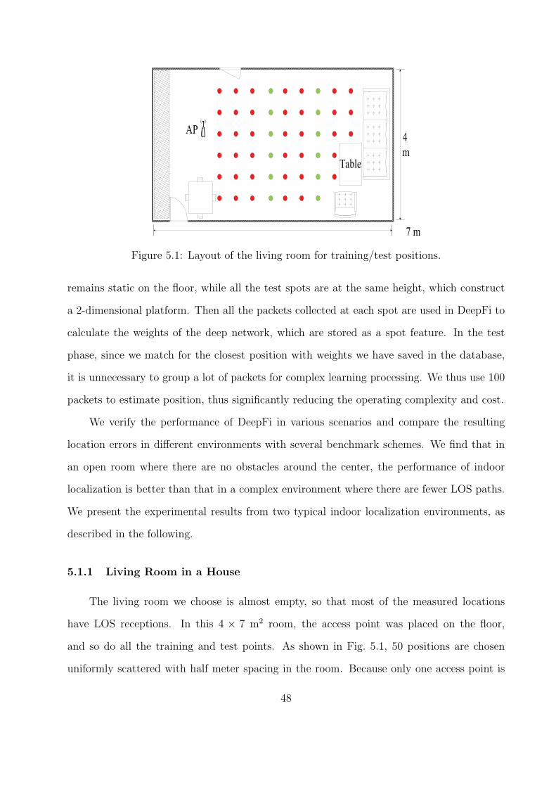
Figure 5.1: Layout of the living room for training/test positions.

remains static on the floor, while all the test spots are at the same height, which construct

a 2-dimensional platform. Then all the packets collected at each spot are used in DeepFi to

calculate the weights of the deep network, which are stored as a spot feature. In the test

phase, since we match for the closest position with weights we have saved in the database,

it is unnecessary to group a lot of packets for complex learning processing. We thus use 100

packets to estimate position, thus significantly reducing the operating complexity and cost.

We verify the performance of DeepFi in various scenarios and compare the resulting

location errors in different environments with several benchmark schemes. We find that in

an open room where there are no obstacles around the center, the performance of indoor

localization is better than that in a complex environment where there are fewer LOS paths.

We present the experimental results from two typical indoor localization environments, as

described in the following.

5.1.1 Living Room in a House

The living room we choose is almost empty, so that most of the measured locations

have LOS receptions. In this 4 × 7 m2 room, the access point was placed on the floor,

and so do all the training and test points. As shown in Fig. 5.1, 50 positions are chosen

uniformly scattered with half meter spacing in the room. Because only one access point is

48

Figure 5.2: Layout of the laboratory for training/test positions.

utilized in our experiment, the access point is placed at one end (rather than the center)

of the room to avoid isotropy. We arbitrarily set 12 positions in two lines as test positions

and use the remaining positions for training (in Fig. 5.1: the training positions are marked

in red and the test positions are marked in green). For each position, we collect CSI data

for nearly 500 packet receptions in 60 seconds. We choose a deep network with structure

K1 = 300, K2 = 150, K3 = 100, and K4 = 50 for the living room environment.

5.1.2 Computer Laboratory

The other test scenario is a computer laboratory in Broun Hall in the campus of Auburn

University. There are many desks and PCs crowded in the 6× 9 m2 room, which block most

of the LOS paths and form a complex radio propagation environment. In this laboratory, 50

training positions and 30 test positions are selected, as shown in Fig. 5.2. The mobile device

will also be put at these locations on the floor, with LOS paths blocked by the desks and

computers. To obtain integrated characteristics of the subcarriers, CSI information for 1000

packet receptions are collected at each location. We choose a deep network with structure

K1 = 500, K2 = 300, K3 = 150, and K4 = 50 for the laboratory environment.

49

Table 5.1: Mean errors for the Living Room and and Laboratory Experiments.

Living Room Laboratory

Method Mean error Std. dev. Mean error Std. dev.(m) (m) (m) (m)

DeepFi 0.9425 0.5630 1.8081 1.3432FIFS 1.2436 0.5705 2.3304 1.0219Horus 1.5449 0.7024 2.5996 1.4573ML 2.1615 1.0416 2.8478 1.5545

5.1.3 Benchmarks

For comparison purpose, we implemented three existing methods, including FIFS [9],

Horus [6], and Maximum Likelihood (ML) [48]. FIFS and Horus are introduced in Chapter 2.

In ML, the maximum likelihood probability is used for location estimation with RSS, where

only one candidate location is used for the estimation result. For a fair comparison, these

schemes use the same measured dataset as in DeepFi to estimate the location of the mobile

device.

The performance metric for the comparison of localization algorithms is the mean sum

error E . Assume the estimated location of an unknown user i is (xi, yi) and the actual

position of the user is (xi, yi). The error of distance estimation is computed as

E =1

N

N∑

i=1

√

(xi − xi)2 + (yi − yi)2. (5.1)

5.2 Localization Performance

We first evaluate the performance of DeepFi under the two representative scenarios.

The mean and standard deviation of the location errors are presented in Table 5.1. In

the living room experiment, the mean distance error is about 0.95 meter for DeepFi with

a single access point. In the computer laboratory scenario, where there exists abundant

multipath and shadowing effect, the mean error is about 1.8 meters across 30 test points.

50

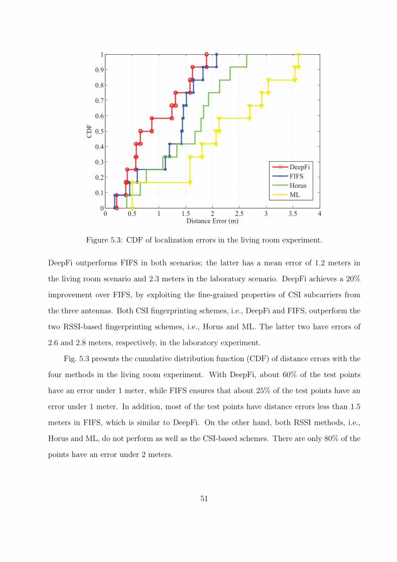
0 0.5 1 1.5 2 2.5 3 3.5 40

0.1

0.2

0.3

0.4

0.5

0.6

0.7

0.8

0.9

1

Distance Error (m)

CD

F

DeepFi

FIFS

Horus

ML

Figure 5.3: CDF of localization errors in the living room experiment.

DeepFi outperforms FIFS in both scenarios; the latter has a mean error of 1.2 meters in

the living room scenario and 2.3 meters in the laboratory scenario. DeepFi achieves a 20%

improvement over FIFS, by exploiting the fine-grained properties of CSI subcarriers from

the three antennas. Both CSI fingerprinting schemes, i.e., DeepFi and FIFS, outperform the

two RSSI-based fingerprinting schemes, i.e., Horus and ML. The latter two have errors of

2.6 and 2.8 meters, respectively, in the laboratory experiment.

Fig. 5.3 presents the cumulative distribution function (CDF) of distance errors with the

four methods in the living room experiment. With DeepFi, about 60% of the test points

have an error under 1 meter, while FIFS ensures that about 25% of the test points have an

error under 1 meter. In addition, most of the test points have distance errors less than 1.5

meters in FIFS, which is similar to DeepFi. On the other hand, both RSSI methods, i.e.,

Horus and ML, do not perform as well as the CSI-based schemes. There are only 80% of the

points have an error under 2 meters.

51

0 1 2 3 4 5 6 70

0.1

0.2

0.3

0.4

0.5

0.6

0.7

0.8

0.9

1

Distance Error (m)

CD

F

DeepFi

FIFS

Horus

ML

Figure 5.4: CDF of localization errors in the laboratory experiment.

Fig. 5.4 plots the CDF of distance errors in the laboratory experiment. In this more

complex propagation environment, DeepFi can achieve a 1.7 meters distance error for over

60% of the test points, which is the most accurate one among the four schemes. Because the

tables obstruct most LOS paths and magnify the multipath effect, the correlation between

signal strength and propagation distance is weak in this scenario. The methods based on

propagation properties, i.e., FIFS, Horus, and ML all have degraded performance than in

the living room scenario. In Fig. 5.4, it is noticed that 70% of the test points have a 3 meters

distance error with FIFS and Horus. Unlike FIFS, DeepFi exploits various CSI subcarriers.

It achieves higher accuracy even with just a single access point. It performs well in this

NLOS environment.

52

5.3 Effect of Different Parameters

5.3.1 Impact of Different Antennas

In order to evaluate the effect of different antennas on DeepFi performance, we consider

two different versions of DeepFi: (i) DeepFi with 90 CSI values from the three antennas as

input data in both phases (3-antenna DeepFi); (ii) DeepFi with only the 30 CSI values from

one of the three antennas in the training phase and estimating the position using 30 CSI

values from the same antenna in the test phase (single antenna DeepFi). In addition, we set

all the other parameters the same as that in the computer laboratory experiments.

In Fig. 5.5, we compare these two schemes for different antennas in the training and

test phases. According to the CDFs of estimation errors for different antennas, it shows that

more than 60% of the test points in the scheme with DeepFi using 90 CSI values from the

three antennas have an estimated error under 1.5 meter, while the other schemes using 30

CSI values from a single antenna have an estimated error under 1.5 meters for fewer than

40% of the test points. In fact, the single antenna scheme has the mean distance error around

2.12 meters for different antennas, while the combined three-antenna scheme has reduced

the mean distance error to about 1.84 meters. Thus, the scheme with 90 CSI values achieves

better localization accuracy than that with 30 CSI values from a single antenna, because the

more environment property of every sampling spot is exploited for location estimation in the

test phase as the amount of CSI values increases from 30 CSI values to 90 CSI values.

Even though the 3-antennas DeepFi scheme achieves a lower mean error, it takes more

time for processing the 90 CSI values as input data for each packet. We evaluate the average

processing time to estimate the device position in the test phase using 100 received packets.

The processing time is measured as the CPU occupation time for the Matlab program running

on a laptop. In Fig. 5.6, we can see that the single antenna schemes take 2.3 seconds on

average to estimate the device position, while the 3-antenna scheme takes around 2.5 seconds

for processing the 100 packets with 90 CSI values per packet as input data to estimate the

53

0 1 2 3 4 5 60

0.1

0.2

0.3

0.4

0.5

0.6

0.7

0.8

0.9

1

Estimated Error (m)

CD

F

Combined three antennasAntenna 1Antenna 2Antenna 3

Figure 5.5: CDF of estimated errors for different antennas.

location. The difference is small, although the latter processes three times input data than

that in the single antenna scheme. Although the 3-antenna DeepFi takes about 10 percent

extra processing time, it can achieve a 15 percent improvement in localization precision. The

latter is generally more important for indoor localization. Considering the tradeoff between

localization precision and time consumption, we select the 3-antenna approach for DeepFi.

5.3.2 Impact of the Number of Packets

In order to study the impact of the number of test packets, we design a specific exper-

iment by utilizing different numbers of packets to evaluate their effect on both localization

accuracy and execution time. In DeepFi, the laptop requests packets from the wireless router

every 50 ms, i.e., at a rate of 20 packets per second. In addition, we assume that a user

randomly moves with the speed of about 1 meter per second, then stays in a 1 meter square

spot for 1 second, moves again, and so forth. Thus 20 packets per second are received for

each test location.

54

Combined Antenna 1 Antenna 2 Antenna 30

0.5

1

1.5

2

2.5

3

Different Antennas

Ave

rage

Exe

cutio

n Ti

me

(s)

Figure 5.6: The average execution time for different antennas.

Fig. 5.7 shows the expectation and the standard deviation of localization error of 90

independent experiments. As the number of test packets is increased, the mean localization

error tends to decrease. For example, the mean estimated localization error is about 1.83

meter for the case of 300 packets, which is better than the error of 1.93 meter for 5 packets.

This is because a large number of test packets provide a stable estimated localization, thus

mitigating the influence of environment noise on CSI values. Another trend is that the

standard deviation of localization error will decrease as the number of packets is increased

due to the fact that as more samples are available, the standard deviation of samples will be

decreased.

In the case of using 5 packets, although it takes less than 1/4 seconds for collecting

them, DeepFi can still achieve a good performance of localization. Apart from reducing the

collecting time, our DeepFi system with 5 packets also simplifies the process of averaging

packets in the test phase, thus significantly reducing the execution time for the online phase.

We compare the average running time of position estimation in the test phase based on

55

5 10 30 100 3000

0.5

1

1.5

2

2.5

The Number of Test Packets

Est

imat

ion

Err

or (m

)

Mean error Standard deviation of error

Figure 5.7: The expectation and the standard deviation of estimation error for differentnumber of packets.

recording CPU occupation time for different packets under 90 independent experiments. In

Fig. 5.8, it can be seen that as the number of packets is increased, the execution time also

increases quickly. This is because our DeepFi system estimates the error of every location by

averaging errors of all packets. For instance, the execution time with 300 packets is around

4.2 seconds, which is about 2.5 times of that with 5 packets (about 1.7 seconds). Therefore,

even though more packets contributes to slightly improving the localization precision, we

prefer to reduce the number of packets for saving collecting and processing time.

5.3.3 Impact of the Number of Packets per Batch

Since deep learning utilizes n packets in the test phase, how to preprocess these packets

is important for DeepFi to reduce the computation complexity. Before the test phase, packets

are divided into several batches, each of which contains a same number of packets. Because

packets are processed in parallel in batches, we can significantly shorten the processing time

56

5 10 30 100 3000

0.5

1

1.5

2

2.5

3

3.5

4

4.5

The Number of Test Packets

Ave

rage

Exe

cutio

n Ti

me

(s)

Figure 5.8: The average execution time of position estimation for different number of packets.

when dealing with a large amount of packets. Here we analyze the impact of the number

of packets per batch. We set 1, 3, 5 and 10 packets per batch for the test phase with 100

collected packets in the experiment. We examine two main effects: the test execution time

and the localization error.

Fig. 5.9 shows that as the number of packets per batch is increased, the average exe-

cution time decreases quickly. If we group 10 packets per batch, 2.3 seconds are needed for

processing 100 packets in the test phase. However, if we decrease the number of packets to 1

packet per batch, which means processing in serial instead of in parallel, it costs 3.5 seconds

to process the same set of packets. Thus, by dividing packets into batches, the computation

time can be effectively reduced. On the other hand, Fig. 5.10 compares the localization

error in the test phase with different numbers of packets per batch. As expected, the four

experiments maintain approximately the same mean and standard deviation of error due to

the fact that the parallel processing based on batches only averages the errors of 100 packets.

57

1 3 5 101.5

2

2.5

3

3.5

4

The Number of Packets per Batch

Ave

rage

Exe

cutio

n Ti

me

(s)

Figure 5.9: The average running time of position estimation for different number of packetsper batch.

Therefore, DeepFi uses 10 packets per batch to reduce the execution time without reducing

localization accuracy.

5.4 Impact of Varying Propagation Environment

Since the CFR changes as the indoor propagation environment varies, we examine the

effect of varying propagation environment on CSI properties through two specific aspects:

replaced obstacles in the room and human mobility. First, because the relative distance

between the transmitter and the obstacle can affect the strength and direction of reflection

of wireless signal, we consider the impact of replaced obstacles at different relative distances.

In the experiment, We place a laptop and a wireless router at two fixed positions, and then

add obstacles at different distances to the router, i.e., at 1 meter, 2 meters, and 3 meters

locations. Then, we calculate and plot the CDF of the correlation coefficient of (i) the 90 CSI

58

1 3 5 100

0.5

1

1.5

2

2.5

The Number of Packets per Batch

Est

imat

ion

Err

or (m

)

Mean error Standard deviation of error

Figure 5.10: The expectation and the standard deviation of estimated error for differentnumber of packets per batch.

values under this cluttered environment and (ii) the 90 CSI values under the obstacle-free

environment.

In Fig. 5.11, we can see that as the distance between the obstacle and the wireless router

is increased, the correlation between the two groups of 90 CSI values becomes stronger, which

means that the obstacle has less impact on wireless signal transmission when it is farther

away. This is due to the fact that when the obstacle is farther from the transmitter, there

is lower possibility that it distorts strong signals such as the LOS signal that the laptop

receives. In addition, more than 80% of the test points have a correlation coefficient greater

than 0.8 when the obstacle is 3 meters away from the wireless router. The high correlation

suggests that the obstacle placed more than 3 meter has no significant impact on the 90 CSI

values the laptop receives. On the other hand, when the obstacle is very close to the router,

the 90 CSI values will slightly change. It leads to a smaller correlation coefficient, which

affects the precision of indoor localization in the test phase based on such CSI properties.

59

−0.8 −0.6 −0.4 −0.2 0 0.2 0.4 0.6 0.8 10

0.1

0.2

0.3

0.4

0.5

0.6

0.7

0.8

0.9

1

Correlation Coefficient

CD

F

Distance = 3 mDistance = 2 mDistance = 1 m

Figure 5.11: CDF of correlation coefficient between 90 CSI values under this environmentwith obstacles and 90 CSI values under that without obstacles.

Therefore, when the obstacle arbitrarily moves in the room, its impact on CSI properties is

acceptable, and high localization precision can still be achieved with DeepFi.

In addition to static obstacles, human mobility is another problem we need to consider

in practical localization. The experiment of human mobility consists of two scenarios: a user

randomly moves (i) near the LOS path, and (ii) near the NLOS path. To demonstrate the

effect of human interference on indoor localization, we also plot the CDF of the correlation

coefficients between (i) the 90 CSI values when a user moves near the LOS path and (ii) the

90 CSI values when a user moves near the NLOS path.

We then present the human mobility experiment results in Fig. 5.12. It can be seen

that there are only fewer than 20% of the test points with a correlation coefficient under

0.7, if a user moves near the LOS path. On the other hand, when a user moves apart from

the LOS path, approximately 20% of the test points has a correlation coefficient under 0.8.

As we can see, the correlation of the two groups of 90 CSI values if a user moves around

the LOS path is weaker than that if a user moves around the reflected path, which is about

60

0.4 0.5 0.6 0.7 0.8 0.9 10

0.1

0.2

0.3

0.4

0.5

0.6

0.7

0.8

0.9

1

Correlation Coefficient

CD

F

Interfere LOSInterfere NLOS

Figure 5.12: CDF of the correlation coefficients between 90 CSI values when a user movesaround and 90 CSI values without human mobility.

2 meter away from the wireless router. In fact, due to the stability of CSI values and high

correlation coefficients for the above two scenarios, the property of the 90 CSI values will

not be significantly affected by human mobility. Therefore, DeepFi can still achieve high

localization accuracy even in a busy environment.

5.5 Impact of the Size of Spot

With DeepFi, a mobile device in the test phase uses 90 CSI values it receives to search

for the most similar training point. Thus, a reasonable localization scheme requires that

each training point possesses unique property of the 90 CSI values. Otherwise, if most of

the points have similar CSI properties, it would be difficult to separate the matched point

and unmatched ones. As a result, these unmatched points, which randomly scatter in the

coverage space, lead to reduce localization accuracy. Therefore, in order to design a suitable

size of spot in our DeepFi system, we study the correlation coefficient of the 90 CSI values

61

between two neighboring points as their interval distance is increased. Our experiment

records many pairs of points with different distances, including 15 cm, 30 cm, 60 cm, and

120 cm. In order to mitigate the effect of the direction of the router on the correlation

coefficient of the 90 CSI values between two points, we equally place the laptop at four

directions facing north, south, west and east.

In Fig. 5.13, it shows that as the size of spot is increased, the correlation coefficient of

the 90 CSI values between two points becomes weaker. In other words, their CSI properties

have less similarity due to the larger size of spots. In fact, as we can see, some points, even

the ones with a shorter space, have low or negative correlation coefficients. This is because

the CFR will change as a user moves over space, as some multipath components may be

blocked at near points and thus some of clusters in received CSI values may be lost. If the

CSI values cannot match the corresponding clusters, the correlation will obviously become

low.

On the other hand, in Fig. 5.13, the performance is acceptable based on the correlation

coefficient for a small spot interval with 30 cm, which means that most test points can match

the training points within the 30 cm range. We thus set the size of the spot for training

points at around 50 cm so that the test point has about 50×√2/2 = 35 cm distance to the

center of the corresponding training point in the spot in the worst case. Otherwise, a larger

size of spot fails to match high similar points because of the scarcity of matched points, while

a smaller size of spot requires redundant pre-training work.

62

−0.5 0 0.5 10

0.1

0.2

0.3

0.4

0.5

0.6

0.7

0.8

0.9

1

Correlation Coefficient

CD

F

15 cm30 cm60 cm120 cm

Figure 5.13: CDF of correlation coefficient of 90 CSI values between two adjacent points.

63

Chapter 6

Conclusions and Future Work

6.1 Summary

We investigated effective indoor localization in this thesis. We first reviewed related

work on indoor localization by classifying the related work into three categories, including

fingerprinting-based, ranging-based, and AOA-based, and discuss each category in detail.

We then presented DeepFi, a deep learning based indoor fingerprinting scheme that uses

CSI information. In DeepFi, CSI information for all the subcarriers from three antennas

are collected from accessing the device driver and analyzed with a deep network with four

hidden layers. Based on three hypotheses on CSI, we proposed to use the weights in the

deep network to represent fingerprints, and incorporated a greedy learning algorithm to train

all the weights layer-by-layer to reduce complexity. In addition, a probabilistic data fusion

method based on the radial basis function was developed for online location estimation. The

proposed DeepFi scheme was validated in two representative indoor environments, and was

found to outperform several existing RSSI and CSI based schemes in both experiments. We

also examined the effect of different parameters including different antennas, the number of

packets, and the number of packets per batch on the DeepFi performance. Finally, we exper-

imented with DeepFi under varying propagation environments, such as obstacles placed at

various locations and human mobility, and found that DeepFi can achieve good performance

under both scenarios.

64

6.2 Future Work

Even though DeepFi can provide high accuracy for indoor localization, there are still

rooms for improvement. In the future, we plan to consider the following three aspects for

performance enhancement.

In this thesis, we train deep network using integrated CSI, including absolute values

and angles, but have not fully utilized the phase information of the CSI data yet. Phase

information can provide at least two applications. First, when the antenna elements are

placed at half of wavelength intervals, the phase difference between two antennas implicitly

indicate the information of signal’s AOA. Second, since the 30 sub-carriers contain 30 pieces

of phase information at different frequency, we can utilize this diversity for training to achieve

better accuracy.

With fingerprinting based localization, we have to create a huge fingerprint database in

the offline phase, where each data unit consists of the CSI and the corresponding position.

Abundant collections are required to prevent underfitting. In the future work, we plan to

apply semi-supervised learning in DeepFi, which makes use of unlabeled data for training.

Instead of labeling all the CSI with exact position, most of data can only have the nearest

position, which can be helpful for feature learning. Since unlabeled data can be collected

when mobile users randomly move around, semi-supervised learning can significantly reduce

the CSI collecting effort in the offline phase.

Another effective method is online machine learning, which we plan to adopt in DeepFi

in the future to reduce the fingerprinting effort. Unlike batch learning, which goes through

the entire training dataset and updates only once, online learning updates the mapping when

processing every new data point. Therefore, instead of completing the training network with

the entire dataset in one shot at the beginning, we can update the mapping when we collect

new data by any mobile user who walks in the room. In order to predict position from which

we have not collected data, we can utilize regression to make a prediction. Therefore, by

65

updating mapping training during walking, we don’t need to collect the entire dataset before

providing the localization service.

66

Bibliography

[1] H. Liu, H. Darabi, P. Banerjee, and L. Jing, “Survey of wireless indoor positioningtechniques and systems,” IEEE Trans. Syst., Man, Cybern. C, vol. 37, no. 6, pp. 1067–1080, Nov. 2007.

[2] X. Wang, S. Mao, S. Pandey, and P. Agrawal, “CA2T: Cooperative antenna arraystechnique for pinpoint indoor localization,” in Proc. MobiSPC 2014, Niagara Falls,Canada, Aug. 2014, pp. 392–399.

[3] P. Bahl and V. N. Padmanabhan, “Radar: An in-building RF-based user location andtracking system,” in Proc. IEEE INFOCOM’00, Tel Aviv, Israel, Mar. 2000, pp. 775–784.

[4] S. Dayekh, “Cooperative localization in mines using fingerprinting and neural networks,”in Proc. IEEE WCNC’10, Sydney, Australia, Apr. 2010, pp. 1–6.

[5] Z. Wu, C. Li, J. Ng, and K. Leung, “Location estimation via support vector regression,”IEEE Trans. Mobile Comput., vol. 6, no. 3, pp. 311–321, Mar. 2007.

[6] M. Youssef and A. Agrawala, “The Horus WLAN location determination system,” inProc. ACM MobiSys’05, Seattle, WA, June 2005, pp. 205–218.

[7] K. Wu, J. Xiao, Y. Yi, D. Chen, X. Luo, and L. Ni, “CSI-based indoor localization,”IEEE Trans. Parallel Distrib. Syst., vol. 24, no. 7, pp. 1300–1309, July 2013.

[8] D. Halperin., W. J. Hu., A. Sheth., and D. Wetherall., “Predictable 802.11 packetdelivery from wireless channel measurements,” in Proc. ACM SIGCOMM’10, NEWDELHI, INDIA, Sept. 2010, pp. 159–170.

[9] J. Xiao, K. Wu., Y. Yi, and L. Ni, “FIFS: Fine-grained indoor fingerprinting system,”in Proc. IEEE ICCCN’ 12, Munich, Germany, Aug. 2012, pp. 1–7.

[10] S. Sen, B. Radunovic, R. R. Choudhury, and T. Minka, “You are facing the Mona Lisa:Spot localization using PHY layer information,” in Proc. ACM MobiSys’12, Low WoodBay, Lake District, United Kingdom, June 2012, pp. 183–196.

[11] A. Krizhevsky, I. Sutskever, and G. Hinton, “ImageNet classification with deep convo-lutional neural networks,” in Proc. Neural Information and Processing Systems 2012,Lake Tahoe, NV, Dec. 2012, pp. 1106–1114.

67

[12] X. Wang, L. Gao, S. Mao, and S. Pandey, “DeepFi: Deep learning for indoor finger-printing using channel state information,” in Proc. IEEE WCNC 2015, New Orlean,LA, Mar. 2015, pp. 1666–1671.

[13] Y. Gu, A. Lo, and I. Niemegeers, “A survey of indoor positioning systems for wirelesspersonal networks,” IEEE communications surveys and tutorials, vol. 11, no. 1, pp.13–32, Jan. 2009.

[14] R. Want, A. Hopper, V. Falco, and J. Gibbons, “The active badge location system,”ACM Transactions on Information Systems, vol. 10, no. 1, pp. 91–102, Jan. 1992.

[15] A. Ward, A. Jones, and A. Hopper, “A new location technique for the active office,”IEEE Personal Communications, vol. 4, no. 5, pp. 42–47, Oct. 1997.

[16] N. Priyantha, A. Chakraborty, and H. Balakrishnan, “The Cricket location-supportsystem,” in Proc. ACM Mobicom’00, Boston, MA, Aug. 2000, pp. 32–43.

[17] M. M. Atia, A. Noureldin, IEEE, and M. J. Korenberg, “Dynamic online-calibratedradio maps for indoor positioning in wireless local area networks,” IEEE Trans. MobileComput., vol. 12, no. 9, pp. 1774–1787, Sept. 2013.

[18] W. Au, C. Feng, S. Valaee, S. Reyes, S. Sorour, S. N. Markowitz, D. Gold, K. Gordon,and M. Eizenman, “Indoor tracking and navigation using received signal strength andcompressive sensing on a mobile device,” IEEE Trans. Mobile Comput., vol. 12, no. 10,pp. 2050–2062, Oct. 2013.

[19] S. Yoon, K. Lee, and I. Rhee, “FM-based indoor localization via automatic ngerprintDB construction and matching,” in Proc. ACM MobiSys’13, Taipei, Taiwan, June 2013,pp. 207–220.

[20] L. M. Ni, Y. Liu, Y. C. Lau, and A. P. Patil, “LANDMARC: indoor location sensingusing active RFID,” Wireless networks, vol. 10, no. 6, pp. 701–710, 2004.

[21] S. P. Tarzia, P. A. Dinda, R. P. Dick, and G. Memik, “Indoor localization withoutinfrastructure using the acoustic background spectrum,” in Proc. ACM MobiSys’11,Washington, DC, June 2011, pp. 155–168.

[22] A. Varshavsky, E. Lara, J. Hightower, A. LaMarca, and V. Otsasonl, “GSM indoorlocalization,” Pervasive and Mobile Computing, vol. 3, no. 6, pp. 698–720, Dec. 2007.

[23] M. Azizyan, I. Constandache, and R. R. Choudhury, “Surroundsense: mobile phonelocalization via ambience ngerprinting,” in Proc. ACM Mobicom’09, Beijing, China,Sept. 2009, pp. 261–272.

[24] J. Chung, M. Donahoe, C. Schmandt, I.-J. Kim, P. Razavai, and M. Wiseman, “Indoorlocation sensing using geo-magnetism,” in Proc. ACM MobiSys’11, Washington, DC,Jun. 2011, pp. 141–154.

68

[25] X. Zhang, C. Wu, and Y. Liu, “Robust trajectory estimation for crowdsourcing-basedmobile applications,” IEEE Trans. Parallel Distrib. Syst., vol. 25, no. 7, pp. 1876–1885,July 2014.

[26] Z. Yang, C. Wu, and Y. Liu, “Locating in ngerprint space: wireless indoor localizationwith little human intervention,” in Proc. ACM Mobicom’12, Istanbul, Turkey, Aug.2012, pp. 269–280.

[27] A. Rai, K. K. Chintalapudi, V. N. Padmanabhan, and R. Sen, “Zee:Zero-effort crowd-sourcing for indoor localization,” in Proc. ACM Mobicom’12, Istanbul, Turkey, Aug.2012, pp. 293–304.

[28] M. Alzantot and M. Youssef, “Crowdinside: Automatic construction of indoor floor-plans,” in Proc. ACM SIGSPATIAL GIS’12, Redondo Beach, CA, Nov. 2012, pp. 99–108.

[29] G. Shen, Z. Chen, P. Zhang, T. Moscibroda, and Y. Zhang, “Walkie-markie: Indoorpathway mapping made easy,” in Proc. USENIX NSDI’13, Seattle, WA, Apr. 2013, pp.269–280.

[30] R. Gao, M. Zhao, T. Ye, F. Ye, Y. Wang, K. Bian, T. Wang, and X. Li, “Jigsaw: Indoorfloor plan reconstruction via mobile crowdsensing,” in Proc. ACM Mobicom’14, Maui,Hawaii, Sept. 2014, pp. 249–260.

[31] Y. Zheng, G. Shen, L. Li, C. Zhao, M. Li, and F. Zhao, “Travi-navi: Self-deployableindoor navigation system,” in Proc. ACM Mobicom’14, Maui, Hawaii, Sept. 2014, pp.471–482.

[32] H. Lim, L. C. Kung, J. C. Hou, and H. Luo, “Zero-conguration indoor localization overIEEE 802.11 wireless infrastructure,” Wireless Networks, vol. 16, no. 2, pp. 405–420,Feb. 2010.

[33] X. Wang, H. Zhou, S. Mao, S. Pandey, P. Agrawal, and D. Bevly, “Mobility improvesLMI-based cooperative indoor localization,” in Proc. IEEE WCNC 2015, New Orlean,LA, Mar. 2015, pp. 2215–222.

[34] K. Chintalapudi, A. P. Iyer, and V. N. Padmanabhan, “Indoor localization without thepain,” in Proc. ACM Mobicom’10, Chicago, Illinois, Sept. 2010, pp. 173–184.

[35] K. Wu, J. Xiao, M. G. Y. Yi, and L. M. Ni, “Fila: Fine-grained indoor localization,” inProc. ACM Infocom’12, Orlando, Florida, Mar. 2012, pp. 2210–2218.

[36] H. Liu, Y. Gan, J. Yang, S. Sidhom, Y. Wang, Y. Chen, and F. Ye, “Push the limit ofWiFi based localization for smartphones,” in Proc. ACM Mobicom’12, Istanbul, Turkey,Aug. 2012, pp. 305–316.

[37] R. Nandakumar, K. K. Chintalapud, and V. N. Padmanabhan, “Centaur: Locatingdevices in an ofce environment,” in Proc. ACM Mobicom’12, Istanbul, Turkey, Aug.2012, pp. 281–292.

69

[38] K. Liu, X. Liu, and X. Li, “Guoguo: Enabling ne-grained indoor localization via smart-phone,” in Proc. ACM MobiSys’13, Taipei, Taiwan, Jun. 2013, pp. 32–43.

[39] R. Schmidt, “Multiple emitter location and signal parameter estimation,” IEEE Trans.Antennas Propag., vol. 34, no. 3, pp. 276–280, Mar. 1986.

[40] S. Sen, K. K. J. Lee, and P. Congdon, “Avoiding multipath to revive inbuilding WiFilocalization,” in Proc. ACM MobiSys’13, Taipei, Taiwan, Jun. 2013, pp. 249–262.

[41] J. Xiong and K. Jamieson, “Arraytrack: A ne-grained indoor location system,” in Proc.ACM NSDI’13, Lombard, IL, Apr. 2013, pp. 71–84.

[42] S. Kumar, E. Hamed, D. Katabi, and L. Li, “LTE radio analytics made easy andaccessible,” in Proc. ACM SIGCOMM’14, Chicago, Illinois, Aug. 2014, pp. 211–222.

[43] S. Kumar, S. Gil, D. Katabi, and D. Rus, “Accurate indoor localization with zerostartup cost,” in Proc. ACM Mobicom’14, Maui, Hawaii, Sept. 2014, pp. 483–494.

[44] J. Wang and D. Katabi, “Dude, where’s my card?: RFID positioning that works withmultipath and non-line of sight,” in Proc. ACM SIGCOMM’13, Hong Kong, China,Aug. 2013, pp. 51–62.

[45] F. FAdib and D. Katabi, “Seeing through walls using WiFi!” in Proc. ACM NSDI’13,Lombard, IL, Apr. 2013, pp. 75–86.

[46] G. Hinton and R. Salakhutdinov, “Reducing the dimensionality of data with neuralnetworks,” Science, vol. 313, no. 5786, pp. 504–507, July 2006.

[47] Y. Bengio, P. Lamblin, D. Popovici, H. Larochelle et al., “Greedy layer-wise trainingof deep networks,” Advances in neural information processing systems, vol. 19, p. 153,2007.

[48] M. Brunato and R. Battiti, “Statistical learning theory for location fingerprinting inwireless LANs,” Elsevier Computer Networks, vol. 47, no. 6, pp. 825–845, Apr. 2005.

70