design of indoor positioning systems based on location...
TRANSCRIPT
DESIGN OF INDOOR POSITIONING SYSTEMS
BASED ON LOCATION FINGERPRINTING
TECHNIQUE
by
Kamol Kaemarungsi
B. Eng., King Mongkut’s Institute of Technology at Ladkrabang,
Thailand, 1994
M. S. in Telecommunications, University of Colorado at Boulder,
1999
Submitted to the Graduate Faculty of
the School of Information Science in partial fulfillment
of the requirements for the degree of
Doctor of Philosophy
University of Pittsburgh
2005
UNIVERSITY OF PITTSBURGH
SCHOOL OF INFORMATION SCIENCE
This dissertation was presented
by
Kamol Kaemarungsi
It was defended on
February 16, 2005
and approved by
Prashant Krishnamurthy, Ph. D., Assistant Professor
Richard Thompson, Ph. D., Professor
Joseph Kabara, Ph. D., Assistant Professor
Ching-Chung Li, Ph. D., Professor
Panos Chrysanthis, Ph. D., Professor
Dissertation Director: Prashant Krishnamurthy, Ph. D., Assistant Professor
ii

Copyright c© by Kamol Kaemarungsi
2005
iii
DESIGN OF INDOOR POSITIONING SYSTEMS BASED ON LOCATION
FINGERPRINTING TECHNIQUE
Kamol Kaemarungsi, PhD
University of Pittsburgh, 2005
Positioning systems enable location-awareness for mobile computers in ubiquitous and per-
vasive wireless computing. By utilizing location information, location-aware computers can
render location-based services possible for mobile users. Indoor positioning systems based
on location fingerprints of wireless local area networks have been suggested as a viable so-
lution where the global positioning system does not work well. Instead of depending on
accurate estimations of angle or distance in order to derive the location with geometry, the
fingerprinting technique associates location-dependent characteristics such as received signal
strength to a location and uses these characteristics to infer the location. The advantage
of this technique is that it is simple to deploy with no specialized hardware required at the
mobile station except the wireless network interface card. Any existing wireless local area
network infrastructure can be reused for this kind of positioning system.
While empirical results and performance studies of such positioning systems are pre-
sented in the literature, analytical models that can be used as a framework for efficiently
designing the positioning systems are not available. This dissertation develops an analytical
model as a design tool and recommends a design guideline for such positioning systems in
order to expedite the deployment process. A system designer can use this framework to
strike a balance between the accuracy, the precision, the location granularity, the number of
access points, and the location spacing. A systematic study is used to analyze the location
fingerprint and discover its unique properties. The location fingerprint based on the received
signal strength is investigated. Both deterministic and probabilistic approaches of location
iv

fingerprint representations are considered. The main objectives of this work are to predict
the performance of such systems using a suitable model and perform sensitivity analyses
that are useful for selecting proper system parameters such as number of access points and
minimum spacing between any two different locations.
Keywords: pattern classification, performance, position location system, system design,
wireless local area network.
v
TABLE OF CONTENTS
PREFACE . . . . . . . . . . . . . . . . . . . . . . . . . . . . . . . . . . . . . . . . . xv
I. INTRODUCTION . . . . . . . . . . . . . . . . . . . . . . . . . . . . . . . . 1
A. INTRODUCTION TO THE STUDY . . . . . . . . . . . . . . . . . . . . . 1
B. BACKGROUND OF INDOOR POSITIONING SYSTEMS . . . . . . . . . 2
C. INDOOR POSITIONING SYSTEMS BASED ON LOCATION FINGER-
PRINTING . . . . . . . . . . . . . . . . . . . . . . . . . . . . . . . . . . . 6
D. APPROACHES AND CONTRIBUTIONS . . . . . . . . . . . . . . . . . . 8
E. ORGANIZATION . . . . . . . . . . . . . . . . . . . . . . . . . . . . . . . . 10
II. LITERATURE REVIEW . . . . . . . . . . . . . . . . . . . . . . . . . . . . 11
A. COMMON COMPONENTS OF INDOOR POSITIONING SYSTEMS . . . 11
B. TAXONOMY OF INDOOR POSITIONING SYSTEMS . . . . . . . . . . . 13
1. Sensing Technologies . . . . . . . . . . . . . . . . . . . . . . . . . . . . . 13
2. Measurement Techniques . . . . . . . . . . . . . . . . . . . . . . . . . . 14
3. Location System Properties . . . . . . . . . . . . . . . . . . . . . . . . . 17
C. RELATED INDOOR POSITIONING SYSTEMS . . . . . . . . . . . . . . . 17
D. INDOOR POSITIONING SYSTEMS USING WIRELESS LANS AND LO-
CATION FINGERPRINTING . . . . . . . . . . . . . . . . . . . . . . . . . 20
1. Indoor Environment . . . . . . . . . . . . . . . . . . . . . . . . . . . . . 21
2. Location Fingerprint . . . . . . . . . . . . . . . . . . . . . . . . . . . . . 22
3. Location Estimation Algorithm . . . . . . . . . . . . . . . . . . . . . . . 25
a. Nearest Neighbor Methods . . . . . . . . . . . . . . . . . . . . . . . . 26
b. Neural Network Methods . . . . . . . . . . . . . . . . . . . . . . . . 29
vi
c. Probabilistic Methods . . . . . . . . . . . . . . . . . . . . . . . . . . 31
d. Support Vector Machine Methods . . . . . . . . . . . . . . . . . . . . 33
4. Summary of Existing Indoor Positioning Performance . . . . . . . . . . 35
E. CONCLUSIONS . . . . . . . . . . . . . . . . . . . . . . . . . . . . . . . . . 37
III. PROPERTIES OF RECEIVED SIGNAL STRENGTH . . . . . . . . . 40
A. MEASUREMENT SETUP . . . . . . . . . . . . . . . . . . . . . . . . . . . 40
1. Experimental Design . . . . . . . . . . . . . . . . . . . . . . . . . . . . . 42
B. COLLECTING MEASUREMENT OF RECEIVED SIGNAL STRENGTH 49
1. User’s Effect . . . . . . . . . . . . . . . . . . . . . . . . . . . . . . . . . 49
a. User’s Body . . . . . . . . . . . . . . . . . . . . . . . . . . . . . . . . 49
b. User’s Orientation . . . . . . . . . . . . . . . . . . . . . . . . . . . . 50
2. Make of Wireless Card . . . . . . . . . . . . . . . . . . . . . . . . . . . . 51
a. Impact of Quantization of RSS Values by Wireless Cards . . . . . . . 56
C. STATISTICAL PROPERTIES OF RECEIVED SIGNAL STRENGTH . . 58
1. Distribution of the Received Signal Strength . . . . . . . . . . . . . . . . 58
2. Standard Deviation of the Received Signal Strength . . . . . . . . . . . 63
3. Stationarity of the Received Signal Strength . . . . . . . . . . . . . . . . 64
4. Time Dependency . . . . . . . . . . . . . . . . . . . . . . . . . . . . . . 67
a. Temporal Received Signal Strength Outage . . . . . . . . . . . . . . 70
5. Interference and Independence . . . . . . . . . . . . . . . . . . . . . . . 70
6. Required Number of Samples . . . . . . . . . . . . . . . . . . . . . . . . 72
D. CAUSES OF ERROR IN LOCATION DETECTION . . . . . . . . . . . . 73
1. Randomness of Received Signal Strength Patterns . . . . . . . . . . . . 74
2. Separation of Location Fingerprints . . . . . . . . . . . . . . . . . . . . 75
3. Separation by Path Loss in Signal Propagation . . . . . . . . . . . . . . 80
E. SUMMARY OF ANALYSIS RESULTS . . . . . . . . . . . . . . . . . . . . 82
F. IMPLICATION ON MODELING OF LOCATION FINGERPRINT . . . . 84
G. CONCLUSIONS . . . . . . . . . . . . . . . . . . . . . . . . . . . . . . . . . 85
IV. MODELING OF THE POSITIONING SYSTEM . . . . . . . . . . . . . 87
A. MODEL FROM PATTERN CLASSIFICATION . . . . . . . . . . . . . . . 88
vii
1. Probabilistic Approach with Lognormal Assumption . . . . . . . . . . . 90
2. Euclidean Distance with Lognormal Assumption and Identity Covariance 94
B. PROBABILITY OF RETURNING THE CORRECT LOCATION . . . . . 99
1. Alternate Calculation of Probability with the Euclidean Distance . . . . 101
2. Extension to Multi-Location Systems . . . . . . . . . . . . . . . . . . . . 103
C. PERFORMANCE EVALUATION . . . . . . . . . . . . . . . . . . . . . . . 105
1. System Model Setup . . . . . . . . . . . . . . . . . . . . . . . . . . . . . 105
2. Results of the Probability of Returning the Correct Location for a Single
Neighbor . . . . . . . . . . . . . . . . . . . . . . . . . . . . . . . . . . . 108
3. Results of the Probability of Returning the Correct Location for Multiple
Neighbors . . . . . . . . . . . . . . . . . . . . . . . . . . . . . . . . . . . 111
D. ERROR DISTANCE DISTRIBUTION . . . . . . . . . . . . . . . . . . . . 112
E. GOODNESS OF ANALYTICAL AND SIMULATION MODELS . . . . . . 115
1. Missing Signals . . . . . . . . . . . . . . . . . . . . . . . . . . . . . . . . 116
2. Non Uniform Grid Spacing . . . . . . . . . . . . . . . . . . . . . . . . . 117
3. Continuity of Real Location . . . . . . . . . . . . . . . . . . . . . . . . . 118
F. CONCLUSIONS . . . . . . . . . . . . . . . . . . . . . . . . . . . . . . . . . 119
V. SYSTEM DESIGN AND DEPLOYMENT . . . . . . . . . . . . . . . . . 120
A. HIGH LEVEL SYSTEM DESIGN . . . . . . . . . . . . . . . . . . . . . . . 120
1. System Design Issues . . . . . . . . . . . . . . . . . . . . . . . . . . . . 121
B. LOW LEVEL SYSTEM DESIGN . . . . . . . . . . . . . . . . . . . . . . . 124
1. Algorithm Selection . . . . . . . . . . . . . . . . . . . . . . . . . . . . . 124
a. Performance Comparison of Different Positioning Algorithms . . . . . 126
2. Performance Achieving Design . . . . . . . . . . . . . . . . . . . . . . . 128
a. Design Examples Using Proposed System Model . . . . . . . . . . . . 129
C. PROTOTYPE OF INDOOR POSITIONING SYSTEM . . . . . . . . . . . 132
1. Performance Evaluation of Prototype . . . . . . . . . . . . . . . . . . . 134
2. Performance Improvement Guidelines for Prototype System . . . . . . . 138
D. HIGH LEVEL DESIGN GUIDELINES . . . . . . . . . . . . . . . . . . . . 139
1. Design Decision Guidelines . . . . . . . . . . . . . . . . . . . . . . . . . 139
viii
E. CONCLUSIONS . . . . . . . . . . . . . . . . . . . . . . . . . . . . . . . . . 139
VI. CONCLUSIONS AND FUTURE WORK . . . . . . . . . . . . . . . . . . 141
A. CONTRIBUTIONS . . . . . . . . . . . . . . . . . . . . . . . . . . . . . . . 142
B. FUTURE RESEARCH WORK . . . . . . . . . . . . . . . . . . . . . . . . 143
APPENDIX A. FIGURES OF RECEIVED SIGNAL STRENGTH DIS-
TRIBUTION . . . . . . . . . . . . . . . . . . . . . . . . . . . . . . . . . . . . 145
APPENDIX B. TABLES OF STANDARD DEVIATION . . . . . . . . . . . 150
APPENDIX C. TABLES OF VARIANCE AND COVARIANCE . . . . . . 153
APPENDIX D. TABLES OF CORRELATION COEFFICIENT . . . . . . . 154
APPENDIX E. FIGURES OF CORRELOGRAMS . . . . . . . . . . . . . . . 161
APPENDIX F. SUMMARY STATISTICS WITH DIFFERENT NUMBER
OF SAMPLES . . . . . . . . . . . . . . . . . . . . . . . . . . . . . . . . . . . 163
APPENDIX G. FLOWCHARTS OF INDOOR POSITIONING PROTO-
TYPE . . . . . . . . . . . . . . . . . . . . . . . . . . . . . . . . . . . . . . . . 168
APPENDIX H. LOCATION FINGERPRINTS OF PROTOTYPE’S EX-
PERIMENT . . . . . . . . . . . . . . . . . . . . . . . . . . . . . . . . . . . . 171
BIBLIOGRAPHY . . . . . . . . . . . . . . . . . . . . . . . . . . . . . . . . . . . . 173
ix
LIST OF TABLES
1 Summary of location stack . . . . . . . . . . . . . . . . . . . . . . . . . . . 13
2 Properties of location systems . . . . . . . . . . . . . . . . . . . . . . . . . 18
3 Parameter comparison of indoor positioning systems . . . . . . . . . . . . . 35
4 Performance comparison of indoor positioning systems . . . . . . . . . . . . 36
5 Factors that affect RSS fingerprint . . . . . . . . . . . . . . . . . . . . . . . 43
6 Measurable access points on 4th floor in Information Science building . . . 45
7 Access points in Hillman library . . . . . . . . . . . . . . . . . . . . . . . . 48
8 Experimental design and measurement factors . . . . . . . . . . . . . . . . 48
9 Sample mean of RSS (dBm) with different orientations . . . . . . . . . . . . 51
10 List of WLAN cards . . . . . . . . . . . . . . . . . . . . . . . . . . . . . . . 52
11 Measurable RSS range of WLAN cards . . . . . . . . . . . . . . . . . . . . 53
12 Statistics of RSS Measured from Two Lucent Gold Cards . . . . . . . . . . 55
13 Mean of RSS with user over short duration of 5 minutes . . . . . . . . . . . 65
14 Variance of RSS with user over short duration of 5 minutes . . . . . . . . . 65
15 Mean and standard deviation of RSS with user . . . . . . . . . . . . . . . . 66
16 Time dependency of RSS (dBm) from SIS410 with users presence . . . . . . 67
17 Interpretation of correlation coefficient . . . . . . . . . . . . . . . . . . . . . 71
18 Sample statistics in dBm of two different locations . . . . . . . . . . . . . . 76
19 Parameters of central chi-squared distribution . . . . . . . . . . . . . . . . . 96
20 Parameters of non-central chi-squared distribution . . . . . . . . . . . . . . 97
21 RSS fingerprints of indoor location . . . . . . . . . . . . . . . . . . . . . . . 108
22 Comparison of off-line phase and on-line phase . . . . . . . . . . . . . . . . 125
x
23 System design of the prototype . . . . . . . . . . . . . . . . . . . . . . . . . 133
24 Recommended values for location system parameters . . . . . . . . . . . . . 139
25 System design checklist . . . . . . . . . . . . . . . . . . . . . . . . . . . . . 140
26 Standard Deviation from Scenario 1 . . . . . . . . . . . . . . . . . . . . . . 150
27 Standard Deviation from Scenario 2 Part I . . . . . . . . . . . . . . . . . . 151
28 Standard Deviation from Scenario 2 Part II . . . . . . . . . . . . . . . . . . 152
29 Estimated Variance and Covariance in Scenario 1 . . . . . . . . . . . . . . . 153
30 Correlation Coefficient from Scenario 1 . . . . . . . . . . . . . . . . . . . . 154
31 Correlation Coefficient Scenario 2 (Ch.1 and Ch.6) . . . . . . . . . . . . . . 155
32 Correlation Coefficient Scenario 2 (Ch.1 and Ch.11) . . . . . . . . . . . . . 156
33 Correlation Coefficient Scenario 2 (Ch.6 and Ch.11) . . . . . . . . . . . . . 157
34 Correlation Coefficient Scenario 2: Interference Effect . . . . . . . . . . . . 158
35 Correlation Coefficient Scenario 2: Interference Effect . . . . . . . . . . . . 159
36 Correlation Coefficient Scenario 2: Interference Effect . . . . . . . . . . . . 160
37 Summary Statistics of SIS410’s RSS at Location 20 . . . . . . . . . . . . . . 163
38 Summary Statistics of SIS401’s RSS at Location 2 . . . . . . . . . . . . . . 164
39 Summary Statistics of SIS501’s RSS at Location 2 . . . . . . . . . . . . . . 164
40 Summary Statistics of hlg-a-card1’s RSS at Location 1 . . . . . . . . . . . . 165
41 Summary Statistics of hlg-b-card1’s RSS at Location 47 . . . . . . . . . . . 165
42 Summary Statistics of hl2-a-card1’s RSS at Location 33 . . . . . . . . . . . 166
43 Summary Statistics of hl2-b-card1’s RSS at Location 5 . . . . . . . . . . . . 166
44 Summary Statistics of hl4-a-card1’s RSS at Location 13 . . . . . . . . . . . 167
45 Summary Statistics of hl4-b-card1’s RSS at Location 25 . . . . . . . . . . . 167
46 Location Fingerprint of 28 Locations in SIS Building . . . . . . . . . . . . . 172
xi
LIST OF FIGURES
1 Input & Output Relationship of the Research . . . . . . . . . . . . . . . . . 8
2 A functional block diagram of positioning system . . . . . . . . . . . . . . . 12
3 A taxonomy of positioning systems . . . . . . . . . . . . . . . . . . . . . . . 15
4 An example of neuron with non-linear activation function . . . . . . . . . . 29
5 Fourth floor of the IS building with AP’s locations . . . . . . . . . . . . . . 44
6 Location of access points on the 4th floor of IS building . . . . . . . . . . . 46
7 First floor of the Hillman library with APs’ location . . . . . . . . . . . . . 47
8 Effect of user’s body on histograms of the same RSS (SIS410) . . . . . . . . 50
9 Comparing mean RSS of different vendors . . . . . . . . . . . . . . . . . . . 54
10 Comparing standard deviation of different vendors . . . . . . . . . . . . . . 54
11 Resolution of Location Fingerprint . . . . . . . . . . . . . . . . . . . . . . . 56
12 Quatization of RSS . . . . . . . . . . . . . . . . . . . . . . . . . . . . . . . 57
13 Comparing Skewness of different vendors . . . . . . . . . . . . . . . . . . . 60
14 Samples of RSS distribution over five minutes and 26 days . . . . . . . . . . 62
15 Average RSS vs. skewness from three APs in Scenario 1 . . . . . . . . . . . 62
16 Average RSS vs. skewness from six APs in Scenario 2 . . . . . . . . . . . . 62
17 Relationship between RSS and its standard deviation from Scenario 1 . . . 64
18 Relationship between RSS and its standard deviation from Scenario 2 . . . 64
19 Correlograms of RSS within the same hour . . . . . . . . . . . . . . . . . . 66
20 Time series of RSS from three APs . . . . . . . . . . . . . . . . . . . . . . . 67
21 Sample mean of RSS over 24 hours at three different days . . . . . . . . . . 69
22 Sample variance of RSS over 24 hours at three different days . . . . . . . . 69
xii
23 Skewness of RSS over 24 hours at three different days . . . . . . . . . . . . 70
24 Unique property of RSS’s distribution measured from typical WLAN card . 74
25 RSS fingerprints with two elements . . . . . . . . . . . . . . . . . . . . . . . 76
26 Two clusters with frequency of RSS fingerprints with two RSS elements . . 77
27 Separation problem of two locations in Scenario 1 with SIS410 and SIS501 . 78
28 Separation problem of two locations in Scenario 1 with SIS401 and SIS501 . 79
29 RSS fingerprints with three elements . . . . . . . . . . . . . . . . . . . . . . 80
30 Path loss propagation of SIS401 in Scenario 1 . . . . . . . . . . . . . . . . . 81
31 Path loss propagation of hl2-b-card1 in Scenario 2 . . . . . . . . . . . . . . 81
32 PDF of central chi-squared distribution . . . . . . . . . . . . . . . . . . . . 96
33 PDF of non-central chi-squared distribution . . . . . . . . . . . . . . . . . . 97
34 Comparison of the PDFs of central and non-central chi-squared distributions 98
35 Central and non-central chi-squared PDFs with large standard deviation . . 98
36 Effect of Mahalanobis distance on probability . . . . . . . . . . . . . . . . . 100
37 A grid space for an indoor positioning system . . . . . . . . . . . . . . . . . 106
38 Effect of number of access points on probability . . . . . . . . . . . . . . . . 109
39 Effect of RSS standard deviation on probability . . . . . . . . . . . . . . . . 109
40 Effect of path loss exponent on probability . . . . . . . . . . . . . . . . . . 110
41 Effect of grid spacing on probability . . . . . . . . . . . . . . . . . . . . . . 110
42 Effect of RSS standard deviation on probability . . . . . . . . . . . . . . . . 111
43 Effect of path loss exponential probability . . . . . . . . . . . . . . . . . . . 112
44 Effect of grid spacing on probability . . . . . . . . . . . . . . . . . . . . . . 112
45 A grid space for an indoor positioning system with 49 locations . . . . . . . 114
46 Comparison of error distance distributions using simulation . . . . . . . . . 115
47 A uniform grid space of 25 positions . . . . . . . . . . . . . . . . . . . . . . 117
48 Location fingerprints of a uniform grid space of 25 positions . . . . . . . . . 118
49 Comparison of average cumulative distribution of error distance . . . . . . . 127
50 Effect of grid spacing on the probability of returning correct location . . . . 130
51 Effect of number of access point on the error distance distribution . . . . . 131
52 Locations of eight access points around the grid of 25 locations . . . . . . . 132
xiii
53 Positions in Prototype System . . . . . . . . . . . . . . . . . . . . . . . . . 134
54 Error distance distribution (CDF) of prototype . . . . . . . . . . . . . . . . 135
55 Analytical prediction of precision on effect of grid spacing . . . . . . . . . . 136
56 Error distance distribution (CDF) of simulation . . . . . . . . . . . . . . . . 137
57 Error distance distribution (PDF) of prototype . . . . . . . . . . . . . . . . 138
58 Error distance distribution (PDF) of prototype . . . . . . . . . . . . . . . . 138
59 Distribution of AP: SIS410 . . . . . . . . . . . . . . . . . . . . . . . . . . . 145
60 Distribution of AP: SIS401 . . . . . . . . . . . . . . . . . . . . . . . . . . . 146
61 Distribution of AP: SIS501 . . . . . . . . . . . . . . . . . . . . . . . . . . . 146
62 Distribution of AP: hl2-b-card1 (4115) . . . . . . . . . . . . . . . . . . . . . 147
63 Distribution of AP: hl4-a-card1 (F5FC) . . . . . . . . . . . . . . . . . . . . 147
64 Distribution of AP: hl4-b-card1 (F23E) . . . . . . . . . . . . . . . . . . . . 148
65 Distribution of AP: hlg-a-card1 (F261) . . . . . . . . . . . . . . . . . . . . . 148
66 Distribution of AP: hlg-b-card1 (F616) . . . . . . . . . . . . . . . . . . . . 149
67 Distribution of AP: hl2-a-card1 (F618) . . . . . . . . . . . . . . . . . . . . . 149
68 Correlogram of Cisco Card at Location 1 over 5 minutes on 1 Dec 04 . . . . 161
69 Correlogram of D-Link Card at Location 1 over 5 minutes on 1 Dec 04 . . . 161
70 Correlogram of Lucent Gold Card at Location 1 over 5 minutes on 1 Dec 04 162
71 Correlogram of Lucent Silver Card at Location 1 over 5 minutes on 1 Dec 04 162
72 Correlogram of Proxim Card at Location 1 over 5 minutes on 1 Dec 04 . . . 162
73 Correlogram of SMC Card at Location 1 over 5 minutes on 1 Dec 04 . . . . 162
74 Flowchart of Off-line Prototype. . . . . . . . . . . . . . . . . . . . . . . . . 169
75 Flowchart of On-line Prototype. . . . . . . . . . . . . . . . . . . . . . . . . 170
xiv

PREFACE
I would like to dedicate this dissertation to my parents, my wife, and my brother. It has been
a long journey for me and they always give me love and encouragement. I would like to thank
my wife, Saowaphak, who has always been there for me. I am indebted to my advisor Dr.
Prashant Krishnamurthy for his continuous guidance, support and encouragement. Without
his patient, valuable suggestions, and comments, I would not be working on this exciting
research topic. Special thanks are due to all my dissertation committee who spent their
valuable time to help me improve this work. I wish to thanks all my fellow students at the
telecommunications program who provide interesting comments. I gratefully acknowledge
the financial support from the following entities: the National Electronics and Computer
Technology Center of Thailand, the Thai Government, the Telecommunications Program,
the School of Information Science, the Link-to-Learn Project, the Common Wealth of Penn-
sylvania, and the National Science Foundation. In addition, I express my appreciation to
the Microsoft Corporation for their Windows XP’s Driver Development Kit, the Carnegie
Mellon University for the donation of wireless access points and cards, and Anand Balachan-
dran who developed Wireless Research API (WRAPI) of the University of California at San
Diego.
xv
I. INTRODUCTION
A. INTRODUCTION TO THE STUDY
Location awareness is one of the key capabilities in context-aware1 computing. Context-aware
computing is one of the building blocks towards the realization of a ubiquitous2 and perva-
sive3 wireless computing environment or smart space where several computers are embedded
within an indoor environment [2]. Location information can provide additional context for
location-aware mobile stations. The meaning and the relevance of data can be interpreted
differently as the mobile station’s location changes with time [4]. Therefore, indoor location
determination for mobile stations imposes a significant challenge for the success of ubiquitous
and pervasive wireless computing.
Location discovery or location determination refers to a process used to obtain location
information of a mobile station (MS) with respect to a set of reference positions within a pre-
defined space. In the literature, this process is usually termed differently as radiolocation [4],
position location [5], geolocation [6], location sensing [7], or localization [8]. This dissertation
will primarily use position location but all of these terms are used interchangeably through-
out the document. A system deployed to determine or estimate the location of an entity
is called a position location system or positioning system. The term positioning system will
be used to represent the system throughout this document. A wireless indoor positioning
1“Context refers to the physical and social situation in which computational devices are embedded. Onegoal of context-aware computing is to acquire and utilize information about the context of a device to provideservices that are appropriate to the particular people, place, time, events, etc.” [1]
2“Ubiquitous computing enhances computer use by making many computers available throughout thephysical environment, while making them effectively invisible to the user.” [2]
3“Pervasive Computing is a term for the strongly emerging trend toward: 1) Numerous, casually acces-sible, often invisible computing devices, 2) Frequently mobile or imbedded in the environment, and 3)Con-nected to an increasingly ubiquitous network structure.” [3]
1
system refers to a wireless network infrastructure that provides indoor location information
to any requesting end user. A set of coordinates or reference points within the predefined
space is typically used to indicate the physical location of the entity. For instance, the global
positioning system (GPS) uses the latitude, longitude, and altitude as the coordinates of an
entity on the Earth’s surface. On the other hand, an indoor positioning system may combine
a floor number, a room number, and other reference objects to represent an entity’s position.
Note that the term position and location are used interchangeably even though the first term
has a smaller scope than the second term.
The applications of indoor location information are not limited to tracking the location
of users and objects in both emergency and normal situations. Concierge services enable
users to become aware of nearest supporting facilities. For example, in an office automation
system a document can be automatically printed to the closest printer near a mobile user.
If a person wearing a location device is not present at his desk, an incoming phone call can
be forwarded to the nearest telephone set [2]. In the field of robotics, a robot can navigate
by itself using the assistance of an indoor positioning system [8]. Smart home applications
such as multimedia appliances that forward multimedia stream to the nearest video screen
can be achieved with a home positioning system [9]. These examples are just some emerging
location related applications.
First, this chapter presents the background of indoor positioning systems, identifies the
challenges of such systems, and briefly describes indoor positioning systems based on lo-
cation fingerprints. Next, the assumptions of study, the overview of approaches, and the
contributions are presented. Finally, the organization of this dissertation is outlined.
B. BACKGROUND OF INDOOR POSITIONING SYSTEMS
The success of outdoor positioning and applications based on the global positioning system
(GPS) provides an incentive to the research and development of indoor positioning systems.
Unfortunately, the GPS system cannot be used effectively inside buildings and in dense
urban areas due to its weak signal reception when there are no lines-of-sight from a MS to
2
at least three GPS satellites [10]. As a result, indoor positioning systems require alternative
means to detect the MS’s location without relying on the direct radio frequency (RF) signal
from GPS satellites. Infrared, RF, and ultra sound signals are major technologies used
for indoor positioning systems. Different types of sensors4 are required to detect these
electromagnetic signals which have characteristics depending on each location. For instance,
a photo-diode detector is commonly used as a sensor to detect infrared signals. A sensing
process converts these signals into a measurable metric such as distance or angle for later
location determination [6]. Then, the measurable metrics are processed by a positioning
algorithm to estimate the MS’s position [6]. Unlike outdoor areas, the indoor environment
imposes different challenges on location discovery due to the dense multipath5 effect and
building material dependent propagation effect. Thus, an in-depth understanding of indoor
radio propagation for positioning is crucial for efficient design and deployment.
Concurrently, there has been an increasing deployment of wireless local area networks
(WLANs) by many individuals and organizations inside their homes, offices, buildings, and
campuses. The popularity of WLANs opens a new opportunity for location-based services.
The WLAN infrastructure can be applied to provide indoor location service without deploy-
ing additional equipment [13]. A wireless network interface card which has the ability to
measure RF signals can be considered as a kind of sensor device. Location-aware applica-
tions for indoor systems are potentially new emerging value-added services for WLANs and
can possibly become a prevalent and successful technology of the future.
Indoor positioning is an emerging technology that lacks theoretical and analytical back-
ground. Pahlavan et al [6] recognize the need for fundamental study of the characterization
of indoor radio propagation and its impact on the accuracy of such systems. A framework
for system design and performance evaluation is required for the success and the growth of
this technology. Krishnamurthy [4] identifies four areas of challenges in position location in
mobile environment which are performance, cost and complexity, security, and application
4“Sensor is a device that responds to physical stimulus (as heat, light, sound, pressure, magnetism, or aparticular motion) and transmits resulting impulse (as for measurement or operating a control)” [11]
5Multipath is a radio frequency’s phenomenon that is the result of radio signals traveling through multiplereflective paths from a transmitter to a receiver [12]. The received signal’s amplitude, phase, and angle ofarrival can fluctuate due to the multipath effect. These signal fluctuations are termed as multipath fadingin wireless mobile communications.
3
requirements. These issues are summarized as follows.
• Performance: The most important performance metric is the accuracy of the location
information. This is usually reported as an error distance between the estimated location
and the actual mobile location. The report of accuracy should include the confidence
interval or percentage of successful location detection which is called the location preci-
sion. Other essential performance metrics are delay, capacity, coverage, and scalability
of the positioning system. The delay metric refers to the time taken between sensing
of the location to reporting the information. The capacity metric measures the number
of location estimations that a system can process per unit time. The coverage metric
reports the boundary of a space that location information can be estimated. Scalability
is a metric that suggests how well the system performs when it operates with a larger
number of location requests and a larger coverage. All of these performance metrics
depend on the choice of sensing technologies, characteristics of the radio channel and
environment, the bandwidth of sensing signal, system’s infrastructure capabilities, posi-
tioning algorithm, and complexity of signal processing techniques employed to estimate
the location information.
• Cost and Complexity: The cost incurred by a positioning system can come from the
cost of extra infrastructure, additional bandwidth, fault tolerance and reliability, and
nature of deployed technology. The cost may include installation and survey time during
the deployment period. If a positioning system can reuse an existing communication
infrastructure, some part of infrastructure, equipment, and bandwidth can be saved. For
instance, in an in-band positioning system, the existing communication signals can also
be used for location sensing. After the system becomes operational, the extra power
consumption at each mobile can be considered as a cost for the positioning system [14].
The complexity of the signal processing and algorithms used to estimate the location is
another issue that needs to be balanced with the performance of positioning systems.
Trade-offs between the system complexity and the accuracy affects the overall cost of the
system.
• Application Requirements: The major application requirements for the location in-
formation are the granularity, the performance, and the availability. These requirements
4
are different from one application to another. First, the granularity can be subdivided
into temporal granularity and spatial granularity. Temporal granularity determines the
rate at which the location information is requested while spatial granularity determines
the level of detail of location information. Second, the performance requirements can in-
clude any combination of performance metrics discussed above. For example, a concierge
service may not require high accuracy but needs a short delay response. Finally, based
on the type of applications, the location information may be required at different entities
within a wireless network either at the MS itself or at a node within the backhaul net-
work. For example, user tracking may require position information at a centralized server
within the fixed network. Based on the entity that estimates the location information,
there are two approaches for location systems: self-positioning and remote-positioning [4].
The difference between these two approaches will be discussed in Chapter II. Moreover,
the design of positioning systems must take into account issues such as the processing
limitations and the constrained battery life of the MS. Besides the three major require-
ments above, privacy concerns may prevent the availability of the location information
at the centralized node inside the fixed network.
• Security: Location information should be made available only to those with authorized
access. This issue represents the privacy concern of mobile users who do not want to
reveal their location or be tracked. It is closely related to how the system determines the
location information and the type of application. A system similar to the GPS where
each GPS device derives its own position from the GPS satellites can completely secure
the user location information. On the other hand, a location tracking such as the E-911
system [15] with the main purpose to capture the user location can be abused by unau-
thorized groups if there is no security protection in place. Therefore, the location system
should have a security protocol embedded within the system to protect the location in-
formation. Unfortunately, the security of the system is limited by the location sensing
technique. For instance, a positioning system that reuses the communication signals for
the purpose of location detection cannot completely secure the MS’s privacy because of
its active nature.
5
C. INDOOR POSITIONING SYSTEMS BASED ON LOCATION
FINGERPRINTING
The demonstration of a positioning system using existing WLAN infrastructure and location
fingerprinting technique such as the RADAR system [13] shows a promising future for indoor
positioning systems. Utilizing the radio frequency (RF) that is readily available by the
widely adopted WLANs, radio frequency based positioning systems can complement the
data networking service with user positioning and tracking capabilities [13]. The location
fingerprinting refers to a technique that exploits the relationship between any measurable
physical stimulus and a specific location. In the RADAR case, the RF received signal strength
is the stimulus. This type of positioning system does not require specialized hardware other
than the common wireless network interfaces with received signal strength measurement
capability; thus, it is relatively simple to deploy compared to other techniques. Unlike
outdoor counterpart systems which can use angle of arrival (AOA) and time difference of
arrival (TDOA) techniques effectively, indoor positioning systems encounter the problem of
non-line-of-sight and the dense multipath effect that render these two techniques ineffective
or complex for practical implementation [13]. It is also difficult for a MS to always see
three or more access points or base stations in indoor environment, which is essential for
triangulation by AOA and TDOA. Location fingerprinting can also be implemented as a
software-based positioning system which can reduce complexity and cost. Any existing
WLAN infrastructure can be reused for this positioning system. Such positioning systems
are viewed as the most effective and feasible solution for the indoor environment [13, 16, 17],
and have thus become the main focus of this dissertation. Generally, the deployment of
fingerprinting based positioning systems can be divided into two phases.
First, in the off-line or calibration phase, the location fingerprints are collected by per-
forming a site-survey of the received signal strength (RSS) from multiple access points (APs).
The entire area is covered by a rectangular grid of points. The distance between two closest
physical positions is called grid spacing and usually reported in meters or feet. However,
some points may be omitted due to inaccessibility. The RSS is measured with enough sta-
tistics to create a database or a table of RSS patterns on the predetermined points of the
6
grid. The database of RSS patterns is called a radio map in [18]. The vector of RSS values
at a point on the grid is called the location fingerprint of that point.
Second, in the on-line phase, a MS will report a sample measured vector of RSSs from
different APs to a central server (or a group of APs will collect the RSS measurements from
a MS and send it to the server). The server uses a positioning algorithm to estimate the
location of the MS and reports the estimate back to the MS (or the application requesting the
position information). The most common algorithm used to estimate the location computes
the Euclidean distance between the sample measured RSS vector and each fingerprint in
the database. The coordinates associated with the fingerprint that provides the smallest
Euclidean distance is returned as the estimate of the position. Other advanced algorithms
such as neural networks [19] and Bayesian modeling [20] have been introduced for indoor
positioning systems to determine the relationship between samples of RSS and the location
fingerprint in the radio map. A summary of recent development of indoor positioning systems
is discussed in the next chapter.
It is clear from the above discussion that the designer should not start out to do the
site survey without proper system design objectives and guideline. Only a few guidelines
are provided in [21] for the practical deployment of location fingerprinting techniques such
as collecting fingerprints every 3 to 5 meters and installing at least 3 access points. The
other performance improvement suggestion in [21] is that if the performance is not sufficient,
collecting more fingerprints in the location in between previous location fingerprints may
help.
It is a problem of choice as to how many access points are required for the system and
what the minimum distance between physical positions on the grid should be in order to
provide a good position resolution and best system performance. The system parameters
and factors that improve the accuracy and the precision performance are still not clear. This
study shows in a later chapter that increasing the number of positions in the database by
reducing the grid spacing can improve the spatial granularity and the accuracy performance,
but may degrade the precision performance. For large indoor environments with multiple
floors, we need a cost/time effective approach to deploy the positioning system. So far there
is no literature that focuses on investigating an analytical model for this kind of system.
7
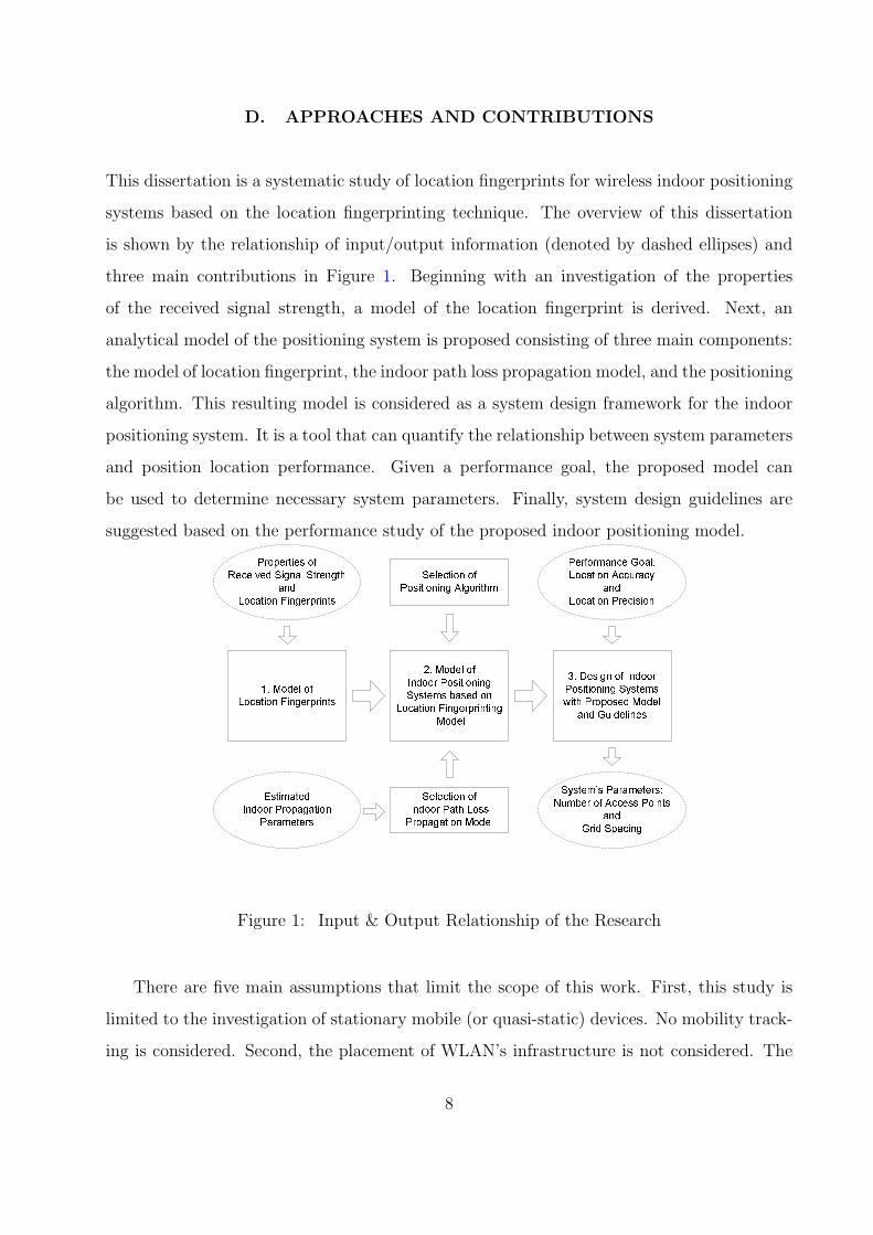
D. APPROACHES AND CONTRIBUTIONS
This dissertation is a systematic study of location fingerprints for wireless indoor positioning
systems based on the location fingerprinting technique. The overview of this dissertation
is shown by the relationship of input/output information (denoted by dashed ellipses) and
three main contributions in Figure 1. Beginning with an investigation of the properties
of the received signal strength, a model of the location fingerprint is derived. Next, an
analytical model of the positioning system is proposed consisting of three main components:
the model of location fingerprint, the indoor path loss propagation model, and the positioning
algorithm. This resulting model is considered as a system design framework for the indoor
positioning system. It is a tool that can quantify the relationship between system parameters
and position location performance. Given a performance goal, the proposed model can
be used to determine necessary system parameters. Finally, system design guidelines are
suggested based on the performance study of the proposed indoor positioning model.Properties ofReceived Signal StrengthandLocation FingerprintsEstimatedIndoor PropagationParameters
Performance Goal:Location AccuracyandLocation PrecisionSystem’s Parameters:Number of Access PointsandGrid Spacing
1. Model ofLocation Fingerprints 2. Model ofIndoor PositioningSystems based onLocation Fingerprinting Model 3. Design of IndoorPositioning Systemswith Proposed Modeland GuidelinesSelection ofPositioning AlgorithmSelection ofIndoor Path LossPropagation Model
Figure 1: Input & Output Relationship of the Research
There are five main assumptions that limit the scope of this work. First, this study is
limited to the investigation of stationary mobile (or quasi-static) devices. No mobility track-
ing is considered. Second, the placement of WLAN’s infrastructure is not considered. The
8
indoor positioning is assumed to be overlaid on top of existing infrastructure. Therefore, the
performance of the positioning system depends on the placement of WLAN infrastructure.
Third, the optimum placement of WLAN’s access points to support indoor positioning is
not included in the scope of current study. Fourth, this study does not consider the search
of an optimal positioning algorithm, but assumes generic algorithms as baseline (such as
the Euclidean distance technique). Finally, hybrid approaches that combine multiple sensor
technologies is beyond the scope of this thesis.
Starting with an analysis of the IEEE 802.11b WLAN’s received signal strength from
measurement experiments, this study performs an extensive data analysis of the location fin-
gerprint in order to understand its underlying features. Properties of the location fingerprints
are investigated in detail. In particular, the distribution of the RSS is considered (whether it
can be approximated by a Gaussian or lognormal distribution). Instead of proposing a new
algorithm or system to supersede existing algorithms or systems, this research provides theo-
retical understanding and concrete recommendations on how to design the indoor positioning
system.
To ensure the success of indoor positioning systems based on location fingerprints, a
theoretical model that can be used as a tool to sufficiently analyze the system is required.
A theoretical framework for analyzing wireless indoor positioning systems based on location
fingerprinting is thus proposed here. A mathematical model is developed to support the
framework by applying the findings of location fingerprints’ properties.
Currently, there are no clear guidelines on how to choose the minimum distance between
physical positions or minimum grid spacing. Moreover, it is not clear how many access points
need to be “heard” at a given location for a given accuracy. A set of system parameters
is identified in this dissertation to aid the designer’s decision before the actual deployment
of the positioning system. A set of guidelines based on an analytical model are developed
so that one could convert a set of performance requirements into a set of system design
parameters. The main goal is to study the accuracy and the precision performance metrics
and suggest a performance evaluation methodology. The result of system analysis can be
applied to streamline the surveying phase such as determining the optimal grid spacing in
order to efficiently deploy the positioning system in indoor areas. The following is the list of
9
contributions:
• Study and characterization of the unique properties of the received signal strength pattern
in location fingerprints through a extensive measurement campaign.
• Proposed a mathematical model for performance analysis of indoor positioning systems
based on location fingerprints using WLANs.
• Identified system parameters used for designing indoor positioning system such as the
grid spacing and the number of access points. Quantified the impact of these system
parameters on the performance of indoor positioning system.
• Recommended design guidelines to facilitate the deployment of indoor positioning system
based on location fingerprinting technique.
• Developed a prototype of software-based indoor positioning system to validate the pro-
posed model.
E. ORGANIZATION
Chapter II reviews the indoor positioning system and provides the justification of the direc-
tion of this research. Chapter III reports on our detailed investigation of the properties of
indoor positioning systems based on the WLAN’s received signal strength. The results in
Chapter III are applied to Chapter IV to model the location fingerprint and the positioning
system. In Chapter V, a set of design guidelines is recommended and the results of indoor
positioning prototype are compared with the results from th proposed model. Finally, the
conclusion and discussion of the future work is presented in Chapter VI.
10
II. LITERATURE REVIEW
This chapter reviews the literature on wireless indoor positioning systems, as a means of pro-
viding an intellectual background for the present research. First in Section II.A, the common
components of indoor positioning systems are described. Then, Section II.B discusses dif-
ferent means to classify indoor positioning systems. Then in Section II.C, related indoor
positioning systems that employ different technologies and techniques are briefly discussed
besides radio frequency based WLANs. Finally, Section II.D reviews all relevant literature
of indoor positioning systems based on location fingerprinting.
A. COMMON COMPONENTS OF INDOOR POSITIONING SYSTEMS
A basic functional block diagram of wireless positioning system is suggested by Pahlavan
et al [6]. It consists of a number of location sensing devices, a positioning algorithm, and
a display system. Figure 2 from [6] illustrates these components and their relationships.
First, the location sensing devices detect the signals transmitted by or received at known
reference points using sensing technologies such as microwave radio frequency (RF), infrared,
or ultrasound. The sensing technique – which can be based on time, direction (angle),
frequency, or signal strength level – converts the sensed signal into location metrics that
are time of arrival (TOA), angle of arrival (AOA), carrier signal phase of arrival (POA), or
received-signal-strength (RSS) [6]. Given a set of known reference points, the relative position
of the mobile station can be derived from the distance or the direction of these location
metrics. Alternatively, the signal characteristics such as RSS at a particular location can form
a pattern unique to that location. Then, the positioning algorithm processes the location
11
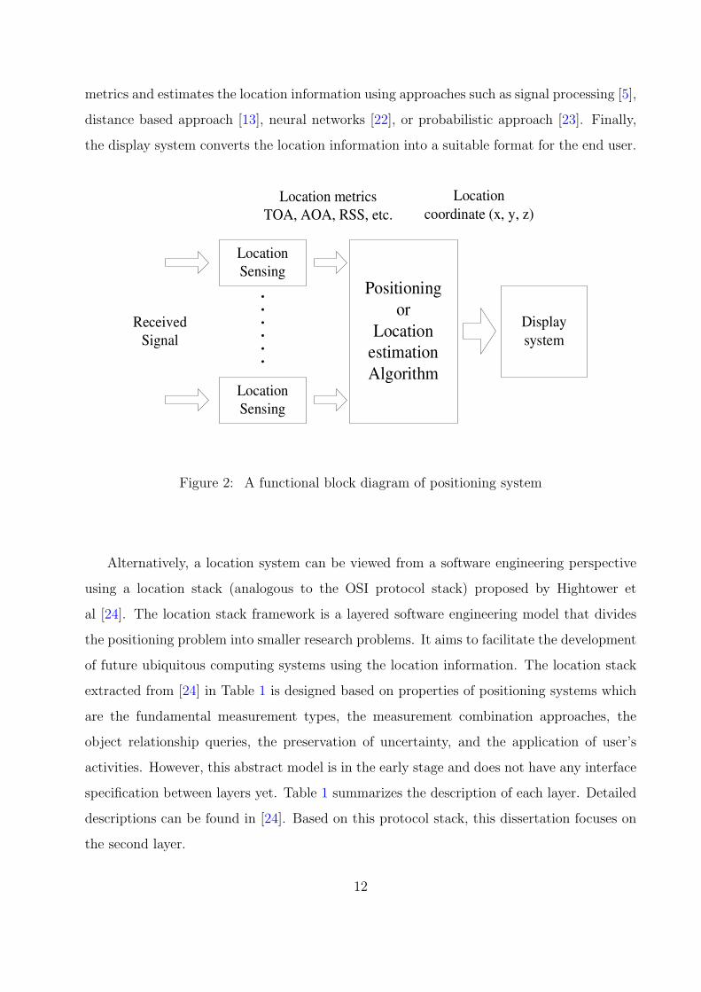
metrics and estimates the location information using approaches such as signal processing [5],
distance based approach [13], neural networks [22], or probabilistic approach [23]. Finally,
the display system converts the location information into a suitable format for the end user.
Location
Sensing
Location
Sensing
Received
Signal
Positioning
or
Location
estimation
Algorithm
Location metrics
TOA, AOA, RSS, etc.
Display
system
Location
coordinate (x, y, z)
Figure 2: A functional block diagram of positioning system
Alternatively, a location system can be viewed from a software engineering perspective
using a location stack (analogous to the OSI protocol stack) proposed by Hightower et
al [24]. The location stack framework is a layered software engineering model that divides
the positioning problem into smaller research problems. It aims to facilitate the development
of future ubiquitous computing systems using the location information. The location stack
extracted from [24] in Table 1 is designed based on properties of positioning systems which
are the fundamental measurement types, the measurement combination approaches, the
object relationship queries, the preservation of uncertainty, and the application of user’s
activities. However, this abstract model is in the early stage and does not have any interface
specification between layers yet. Table 1 summarizes the description of each layer. Detailed
descriptions can be found in [24]. Based on this protocol stack, this dissertation focuses on
the second layer.
12
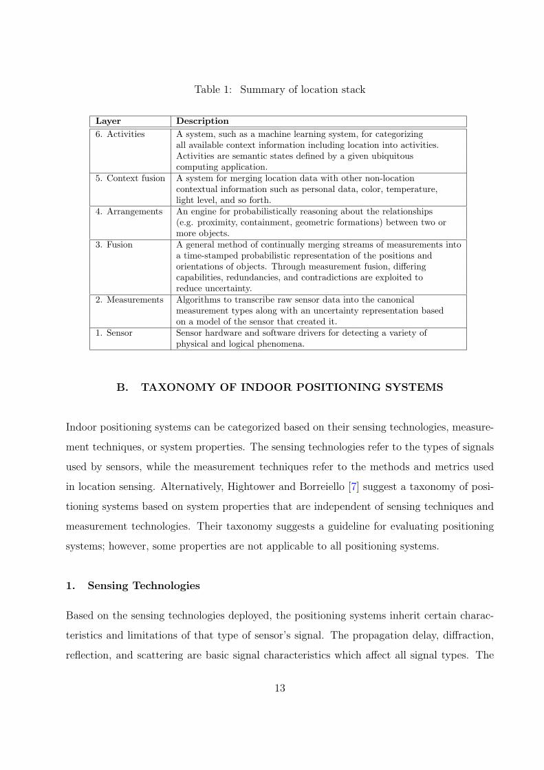
Table 1: Summary of location stack
Layer Description6. Activities A system, such as a machine learning system, for categorizing
all available context information including location into activities.Activities are semantic states defined by a given ubiquitouscomputing application.
5. Context fusion A system for merging location data with other non-locationcontextual information such as personal data, color, temperature,light level, and so forth.
4. Arrangements An engine for probabilistically reasoning about the relationships(e.g. proximity, containment, geometric formations) between two ormore objects.
3. Fusion A general method of continually merging streams of measurements intoa time-stamped probabilistic representation of the positions andorientations of objects. Through measurement fusion, differingcapabilities, redundancies, and contradictions are exploited toreduce uncertainty.
2. Measurements Algorithms to transcribe raw sensor data into the canonicalmeasurement types along with an uncertainty representation basedon a model of the sensor that created it.
1. Sensor Sensor hardware and software drivers for detecting a variety ofphysical and logical phenomena.
B. TAXONOMY OF INDOOR POSITIONING SYSTEMS
Indoor positioning systems can be categorized based on their sensing technologies, measure-
ment techniques, or system properties. The sensing technologies refer to the types of signals
used by sensors, while the measurement techniques refer to the methods and metrics used
in location sensing. Alternatively, Hightower and Borreiello [7] suggest a taxonomy of posi-
tioning systems based on system properties that are independent of sensing techniques and
measurement technologies. Their taxonomy suggests a guideline for evaluating positioning
systems; however, some properties are not applicable to all positioning systems.
1. Sensing Technologies
Based on the sensing technologies deployed, the positioning systems inherit certain charac-
teristics and limitations of that type of sensor’s signal. The propagation delay, diffraction,
reflection, and scattering are basic signal characteristics which affect all signal types. The
13
effective range, available bandwidth, regulatory constraints, interference, power constraints,
safety, and cost are technology limitations [14]. The wireless signals commonly used for
indoor positioning systems are infrared, radio frequency, and ultrasound. Note that other
technologies such as laser ranging, scene analysis, and inertial based systems are also possible
for indoor positioning system, but are beyond the scope of this study. Brief descriptions of
the three major sensing technologies are as follows [14]:
• Infrared: The infrared signal has the same properties as visible light. It cannot pass
through walls or obstructions; therefore, it has a rather limited range in indoor environ-
ments. However, the propagation speed is high, approximately 3 × 10⁸ m/s. Thus, it
requires a more sophisticated circuitry than ultrasound signals. Indoor lighting interferes
with this type of signal and causes problems in accurate sensing. It generally has a range
of around 5 m. The infrared devices are usually small in size compared to ultrasound
devices [25].
• Radio frequency: The radio frequency (RF) signal can penetrate most indoor building
material; therefore, it has an excellent range in indoor environments. The propagation
speed is also high, approximately 3 × 10⁸ m/s. There are unlicensed frequencies avail-
able freely for use. This type of signal has the longest range compared to infrared and
ultrasound.
• Ultrasound: Although ultrasound operates at low frequency bands (typical 40 kHz) com-
pared to the other two signaling technologies, it possesses a good precision for location
sensing at a slow propagation speed of sound (343 m/s). The advantages of ultrasound
devices are their simplicity and that they are inexpensive. However, ultrasound does
not penetrate walls but reflects off most of the indoor obstructions. It has a short range
around 3 m to 10 m but has a 1 cm resolution of distance measurement. The operating
temperature influences the performance of ultrasound.
2. Measurement Techniques
Besides the sensing technologies, wireless positioning systems can be categorized by mea-
surement techniques used to derive the position of mobile stations. The major categories are
14
based on the measurement of distance, angle, location pattern or fingerprint, and any combi-
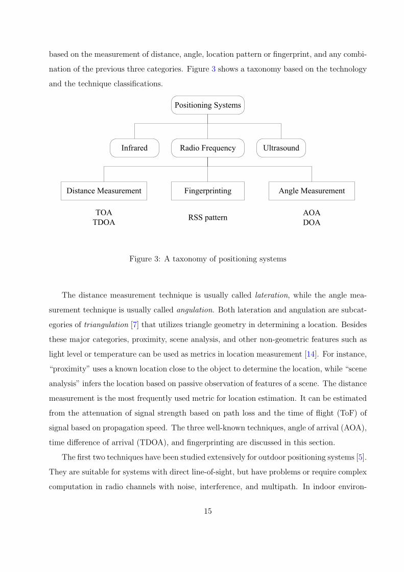
nation of the previous three categories. Figure 3 shows a taxonomy based on the technology
and the technique classifications.
Figure 3: A taxonomy of positioning systems
The distance measurement technique is usually called lateration, while the angle mea-
surement technique is usually called angulation. Both lateration and angulation are subcat-
egories of triangulation [7] that utilizes triangle geometry in determining a location. Besides
these major categories, proximity, scene analysis, and other non-geometric features such as
light level or temperature can be used as metrics in location measurement [14]. For instance,
“proximity” uses a known location close to the object to determine the location, while “scene
analysis” infers the location based on passive observation of features of a scene. The distance
measurement is the most frequently used metric for location estimation. It can be estimated
from the attenuation of signal strength based on path loss and the time of flight (ToF) of
signal based on propagation speed. The three well-known techniques, angle of arrival (AOA),
time difference of arrival (TDOA), and fingerprinting are discussed in this section.
The first two techniques have been studied extensively for outdoor positioning systems [5].
They are suitable for systems with direct line-of-sight, but have problems or require complex
computation in radio channels with noise, interference, and multipath. In indoor environ-
15
ments, the mobile station is surrounded by scattering objects which results in multiple angles
of the signal reception. On the other hand, the distance between transmitter and receiver is
usually shorter than the time resolution that can be measured by the system. Therefore, the
AOA and TDOA approaches are impractical for indoor environments. The fingerprinting
technique has gained more attention lately due to its simplicity compared to the first two for
indoor positioning systems. The descriptions of each measurement techniques are as follows.
• Distance Measurement Based on Time Delay: Time of arrival (TOA) and time difference
of arrival (TDOA) techniques rely on the precision of timing between the signal trans-
mitter and the receiver in order to use the propagation delay or time of flight (ToF) to
calculate the distance between transmitter and receiver. Therefore, a precise synchro-
nization is also very important in such systems. By combining at least three distances
from three reference positions, triangulation can be used to estimate the mobile station’s
location. This type of technique will require a high accuracy clock in the communica-
tion system. TDOA is more practical [5]. Example of location-sensing systems that
use time of flight are GPS [7], the Active Bats [26], and the Cricket [27]. Besides these
time delay-based techniques, the distance between transmitter and receiver can also be
determined from signal strength attenuation and direct distance measurement (such as
dead reckoning).
• Angle Measurement: Angle of arrival (AOA) or direction of arrival (DOA) techniques
locate the mobile station by determining the angle of incident signals. Using simple geo-
metric relationships, the location estimate can be calculated by the intersection of two
lines of bearing (LOBs) which are formed by a radial line from transmitter to receiver [5].
In a two-dimensional plane, at least two reference points are required for location esti-
mation. However, this technique requires the uses of directional antennas and antenna
arrays to measure the angle of incidence. Thus, it is difficult to measure the AOA at the
mobile station.
• Fingerprinting or Location Pattern Matching: This technique generally requires only
measurement of received signal strength or other non-geometric features at several loca-
tions to form a database of location fingerprints. To estimate the mobile location, the
system needs to first measure the received signal strength at particular locations and
16
then search for the pattern or fingerprint with the closest match in the database. This
technique does not require the mobile station to see at least three base stations or access
points in order to determine the location. The disadvantage of this technique is that it
is very time-consuming to perform an exhaustive data collection for a wide area network
such as in outdoor positioning systems.
3. Location System Properties
A set of properties which are independent of sensing technologies and measurement tech-
niques can be used to classify indoor positioning systems. Table 2 lists system properties
based on the survey of location systems in [7]. These properties viewed as another taxonomy
can be used to characterize or evaluate positioning systems [7]. An additional property is
added based on the type of services that positioning systems can provide [28].
C. RELATED INDOOR POSITIONING SYSTEMS
Excellent comprehensive surveys of positioning systems can be found in [7] and with a special
focus on indoor positioning systems in [14]. Therefore, this section will not delve into greater
details of each of the forerunners of indoor positioning systems. A subset of these systems
is reviewed as examples. The major characteristics of these systems are summarized.
• The Active Badge location system [25] is one of the first generation of indoor positioning
systems. A central server determines user’s locations using sensors to pick up periodically
transmitted or on demand signals from infrared badges attached to the mobile user. The
infrared signal of each user has a unique identifier. The location determination is based
on the proximity of the badge and the cellular-based sensor; therefore, only symbolic
location information at room-sized granularity is available. This system has limited
range and the infrared signal is susceptible to interference from sunlight and fluorescent
lights [7].
• The second location system called Active Bat [26] improves the accuracy over Active
17

Table 2: Properties of location systems
Property DescriptionPhysical Position v.s. Symbolic Location - Physical position or abstract reference is
based on analytic labeling or coordinationsuch as latitude, longitude, and altitude.- Symbolic location or real world referenceis based on proximity of known objects orabstract ideas of location
Absolute or Relative Referencing - Absolute referencing systems share singleor unified reference grid.- Relative referencing systems have their ownframe of reference grid for each locator.
Remote or Local Computation - Remote computing systems estimate location(Network- or Mobile-based) of mobile station by network of location
systems or backhaul positioning server. Thisis also called network-based system.- Local computing systems estimate their ownlocation, e.g. self-positioning. This is alsocalled mobile-based system.
Network- or Mobile-Assisted This indicates the sensing side which is doneseparately from the location computation side.
Recognition Capability Some positioning systems inherit recognitioncapability that can classify or identifylocated objects such as global ID or naming.
Accuracy and Precision - Location accuracy is usually reported inmeters as an error distance in the estimatedlocation that deviates from the correctlocation.- Location precision is usually reported inpercentage of correct estimation at certainaccuracy.
Cost and Time - Cost of deploying a location system consistsof the installation cost, infrastructure cost,user terminal or device cost, and time cost.- Time to deploy the system: installation time,and time to estimate the location.
Scalability The scope of space, time, frequency, andcomplexity of positioning system may limit thescalability.
Security and Privacy - Security prevents unauthorized use of locationinformation.- Privacy ensures anonymity of the user.
Service Categories Mobile location-based applications can beclassified as either business-to-consumer (B2C)or business-to-business (B2B) [28].
18
Badge by utilizing both radio and ultrasound signals. The distance measured (used
in lateration computation at a centralized controller) is calculated from the time-of-
flight of the ultrasound signal. The location system consists of a set of ceiling-mounted
receivers that detect the ultrasound signal from the Active Bat tag that responds to
an RF request packet from the centralized controller. The ceiling-mounted receivers,
which are connected to the centralized controller via a wired serial network, calculate
the distance measurement starting from the time they receive a reset signal in wired
network to the time they receive ultrasound pulse from the mobile “Bat”. The accuracy
and the precision are quite impressive at 9 cm for 95% of locations.
• The SpotON ad hoc location system [29] is another positioning system that uses distance-
based measurement, but the distance is derived from signal strength attenuation instead
of time-of-flight. The system designers combine the ideas of ad hoc networking and
object localization together. Each object to be located is attached with an RF tag. Ad
hoc lateration is performed using the estimated inter-tag distance instead of the distance
from known sensors or base stations. Therefore, the system could provide both relative
and absolute referencing. A dynamic cluster of tags enables any participating node to
exploit correlation of multiple measurements and improves the location accuracy as the
tags’ cluster becomes denser [29].
• Cricket location-support system [27] is a location-based system designed with four objec-
tives: privacy, decentralization, low cost, and room-sized granularity. The system is said
to be independent of data network technology. It has no centralized server; therefore, the
mobile device has to calculate its own location using both ultrasound and RF technolo-
gies. The mobile device measures the ultrasound signal in order to calculate the range
with TDOA techniques while the RF signal is used for synchronization and to identify
the period of the ultrasound signal. Each room is equipped with a beacon that transmits
an RF pulse with a unique ID for that particular room. This mobile-based approach
ensures its privacy. However, there are potential errors from RF beacon interference that
cause confusion between two adjacent rooms.
• PinPoint’s 3D-iD local positioning system [30] is an indoor RF-based commercial product.
It determines the location of a tag by continuously broadcasting a signal from an array
19
of antennas at known cells’ positions. Upon receiving a signal, the tag will immediately
retransmit the message by shifting to it another radio frequency and encoding it with its
own ID. The system controller measures multiple distances from the array of antennas
using RF round-trip time and performs multilateration. The signal from a transmitter
cell (called cell controller) is a spread-spectrum signal operating at 2.4 GHz with 40 MHz
bandwidth, while the tag transmits a response signal at 5.78 GHz. The system has a
30 m range and 1 m to 3 m accuracy. This system requires several cell controllers per
building and has expensive hardware.
These pioneer works in this area have some disadvantages such as the limitation of the
infrared or ultrasound sensing signals that cannot penetrate the walls and floors which are
common inside most buildings. The cost of sensor infrastructure installation and badges or
tags for most of these systems becomes significant for a building with a lot of small rooms
or offices. Notice that the angular or direction-based measurement was not used in any of
these systems due to the dense multipath effect inside buildings. However, these position-
ing systems have only demonstrated their success empirically, and they all lack theoretical
explanation of their system and performance.
D. INDOOR POSITIONING SYSTEMS USING WIRELESS LANS AND
LOCATION FINGERPRINTING
This section reviews relevant RF-based indoor positioning systems which can be used to
locate stationary objects and track mobile users. The impressive growth of IEEE 802.11
wireless LANs (WLANs) in recent years suggests an interesting future for the location fin-
gerprinting technique. This type of positioning system can be overlaid on top of any existing
WLAN; therefore, it can save the cost of dedicated infrastructure. Moreover, it utilizes ra-
dio frequency signals which can penetrate most of the indoor materials resulting in a larger
range and reducing the number of required access points for positioning purposes. Because
the RSS can be measured by all WLAN network interface cards, no dedicated tag or badge is
required for some of the current laptops and PDAs with built-in IEEE 802.11 interface. The
20
system is quite flexible because system designers can select whether to have a centralized
positioning server or let the mobile determine its own position. However, the fingerprinting
technique requires a training phase (off-line phase) to collect location fingerprints for all
positions in the operating area, before the actual deployment (on-line phase).
After a number of empirical and feasibility studies such as in [13, 31], recent develop-
ment has been focused on improvement of location estimation algorithms and system per-
formance [8, 23, 22, 18]. Popular machine learning techniques such as neural network and
support vector machines (SVMs) have been introduced to improve the performance with
RSS fingerprinting.
The following discussion is divided according to the positioning system components out-
lined in Section II.A. First, the effects of the environment on the RF signals such as the
radio channel and the user’s presence are discussed. Second, the common form of location
fingerprint and its relationship with physical position are explained. Third, a number of lo-
cation estimation algorithms are reviewed. Finally, the performance of existing positioning
systems are compared.
1. Indoor Environment
The indoor environment has unique properties that influence the radio frequency signals
used by the sensors of positioning systems. The prominent phenomena is the multipath
effect which dominates how the received signals behave for all wireless receivers. Although
there are several studies on indoor radio propagation and modeling, this section discusses only
the studies focused on indoor positioning systems. The study in [32] at the Carnegie Mellon
University showed the results of their fixed WLAN station measurement inside an office
building. Different periods of measurement were performed to determine the distribution
of WLAN received signal strength. Their conclusion pointed out that since the mean, the
median, and the mode of the data collected at a single location were very close together, the
distribution was lognormal. Besides the distribution, the relationship between the range and
the standard deviation shows linear dependence and a larger transmitter-receiver distances
corresponds to a larger range of standard deviation. Their study also briefly mentioned the
21
effect of time of day where they showed that there are negligible differences between different
times of day on their received signal data. However, most of their results and conclusions
are questionable, based on our exhaustive studies discussed in Chapter III.
Another study in [8] also briefly discusses the distribution of received signal strength.
Although their duration of measurement is rather short compared to the study at Carnegie
Mellon, the results contradict the traditional belief of lognormally distributed of received
signal strength. The authors in [8] pointed out that most measured signal distributions are
multi-modal1 with a dominant mode2 and asymmetric3.
Another important factor that affects the received signal is the user’s body which could
block the signal path during the operation. Water, which has a resonance frequency at
2.4GHz and is a significant part inside the human body, greatly attenuates the WLAN
signal strength [8, 18]. In some location-based applications such as in robotics and other
non-human related service, the effect of user’s presence should be neglected. The RADAR
system in [13] suggested that the user’s orientation affected average received signal strength
for the access point blocked by the user. Therefore, the orientation should be included in
the location information. The human being’s movement inside the building creates random
effects of radio propagation inside the building [31]. The other uncontrollable factors, which
are the temperature, air movement, and interference from other devices operating in the
same frequency, also cause the received signal at any particular location to fluctuate over
time [31]. However, in the literature, there is no good characterization of the properties of
the RSS with the indoor positioning applications in mind.
2. Location Fingerprint
A location fingerprint based on RF characteristics such as RSS is the basis for representing a
unique position or location. It is created under the assumption that each position or location
inside a building has a unique RF signature [6]. Generally, a fingerprint F is labeled with a
location information L. The location fingerprints and their labels (e.g. location information)
1Mode is the most likely value that has the highest probability in a set of observations. There may bemore than one mode in any set of observations and it is called multi-modal [33].
2Example of a distribution with a dominant mode is shown in lower right sub-graph of Figure 14.3Asymmetric distribution is a distribution that has different shape on both side of its mode.
22
are maintained in database and used during the on-line phase to estimate the location. The
label and fingerprint are usually denoted as a tuple of (L,F). The measurement dataset
collected during the off-line phase is called a training set4.
Battiti et al [22] point out that the location information L for indoor location can be
recorded in two forms as either a tuple of coordinates or an indicator variable. The tuple
of real coordinates can vary from one dimension to five dimensions which includes the three
dimension space and two orientation variables expressed in spherical coordinates [22]. For
instance, a location information of a two-dimension system with an orientation could be
expressed as a triplet L = {(x, y, d) | x, y ∈ R2, d ∈ {North,East,South,West}}. In the case
of the indicator variable, the scope of location covers a wider area such as a room. The
indicator variable reports only a rough granularity whether the object is inside or outside
the area. An example is given by [22] as L = {−1, 1}. Indoor location systems that use
coordinates are said to be solving a regression problem, while the systems that use indicator
variables are said to be solving decision or classification problems.
It is commonly acknowledged that the RSS is the simplest and most effective RF signature
for location fingerprints because it is readily available in all WLAN interface cards. The RSS
was found by [13] to be more location-dependent than the signal-to-noise ratio (SNR) because
the noise component is rather random in nature. However, the RSS itself fluctuates over time
for each access point and location. Each RSS element can be considered as a random variable;
therefore, it can be captured by recording its descriptive statistics parameters, approximating
its distribution, or maintaining the whole measurement dataset. These approaches of RSS
representation result in different procedures for location estimation algorithms in the next
subsection. Regardless of the approach, the location fingerprint is usually denoted as an array
or vector of signal strength (random variables) received at any position in the location-based
service area. The size of the vector is determined by the number of access points that can
be heard.
To create a basis fingerprint such as in [13, 31], a number of samples of vectors of
signal strength are collected over a window of time for each position. This basis is called
a prototype [34]. Then, the average RSS of each access point is calculated and recorded as
4according to the learning theory [22]
23
an element in the location fingerprint. For an area that can receive signals from N access
points, the location fingerprint can be expressed as a vector of average RSS elements ρi:
F = (ρ1, ρ2, . . . , ρN)T . (II.1)
Extra fingerprint information such as standard deviation for each RSS element, which is
suggested in [31], may be added into the location fingerprint as another vector of standard
deviations:
D = (σ1, σ2, . . . , σN)T . (II.2)
An alternative approach to location fingerprints is investigated by [8, 23] in which the
probability distribution is estimated for the RSS signature at a given location. The location
fingerprint becomes a conditional probability distribution of the form P (F | L) where F de-
notes the observation vector of RSS and L denotes the location information. The conditional
probability P (F | L) is called the likelihood function because it provides the probability or
probability density of the occurrence of the RSS vector given the known location informa-
tion [23]. With this form of location fingerprint, the Bayes’ rule can be used to estimate the
location. Details of Bayesian algorithms for location estimation are discussed in the next
subsection.
The examples of location fingerprinting explained above suggest that there are two ways
to model the relationship or dependency between the location information and the RSS
signature. The first way where the location information is tied to the constant value of
average RSS vector is called deterministic approach. The second way where the probabilistic
dependency is exploited is called the probabilistic approach.
Besides the basis location fingerprint, the samples of location fingerprint measured during
the on-line phase is also important for the system that tracks the mobile object. The time
interval and number of samples should be selected appropriately to represent the location
fingerprint for the mobile application.
A step in statistical analysis method called preprocessing [35] is another important issue
needed to be considered because it can impact the estimation of dependency between location
fingerprint and the location information easier. The preprocessing refers to a step that cleans
the raw data (in this case the training set) before any further operations or analysis. The
24
cleaning may consist of encoding, dimensionality reduction (reduce unnecessary elements),
feature extraction/selection, clustering [35], and outlier elimination [31]. Roos et al point
out that the preprocessing enables faster location estimation and reduces the noise from the
training data. The process that creates the basis of location fingerprint discussed above
could be considered as a part of preprocessing [23]
3. Location Estimation Algorithm
Location estimation algorithms or positioning algorithms are procedures that exploit depen-
dency between location information and location fingerprint basis in order to determine a
position or location from samples of RSS signals. The examples of simple location estimation
algorithms are strongest base station selection method and random selection method. The
strongest base station selection assumes that the current user’s position is closer to the base
station that has the strongest signal strength, while the random selection reports the user’s
position at random from a set of known positions [13]. It is obvious that these two algo-
rithms may not provide satisfactory results. More complex algorithms can take advantage of
the dependency between RSS fingerprint and location information and could provide better
accuracy, precision, and granularity of the location information.
From a machine learning perspective, the positioning algorithms are pattern classifiers
because they are procedures that can automatically separate samples of patterns into dif-
ferent classes [23]. Each class is referred to as a class of RSS patterns that comes from the
same location or position. The algorithms estimate the location or position from samples
of RSS vectors by learning from previous examples of location-dependent RSS fingerprints
or signatures. The previous RSS data or training set are used to calibrate estimator models
that can automatically relate location fingerprints and location information.
In the literature, positioning algorithms can be classified into deterministic and proba-
bilistic types based on the approaches that model the relationship between location finger-
prints and location information as discussed in previous subsection. The deterministic type
of algorithms are those that based on the nearest neighbor classifiers and neural network
classifiers. The probabilistic type of algorithms are those that are based on the Bayesian in-
25
ference and statistical learning theory such as support vector machines (SVMs). The major
algorithms for indoor positioning systems are discussed below.
a. Nearest Neighbor Methods The nearest neighbor methods are deterministic algo-
rithms because they require only a set of constant location fingerprints which includes mean
vectors and standard deviation vectors of RSS. In order to determine the location, a form
of discriminant function is commonly used to classify a sample of RSS fingerprint into a
position. These nearest neighbor methods are also called case-based methods [23] because
they classify each position into a case or class.
The mean or average RSS vector is a center of a mass which represents each class of
location fingerprint. The basic algorithm for the nearest neighbor classifier is that it selects
the class or case based on the closeness of a sample fingerprint to the center of the mass of
that particular location fingerprint. Suppose that a set of l location fingerprints is denoted
by {F1,F2, . . . ,Fl} exist and each fingerprint has a one-to-one mapping to a set of positions
{L1,L2, . . . ,Ll}. A sample of an RSS fingerprint measured during an on-line phase is denoted
as S which can be another mean or average RSS vector of a small window of RSS samples.
Assuming that an indoor positioning system only considers the average RSS from N access
points as a location fingerprint, the sample of RSS vector is S = (s1, s2, . . . , sN)T and each
location fingerprint i in the database can be expressed as Fi = (ρi1, ρ
i2, . . . , ρ
iN)T .
The simplest closeness metric is a distance measurement in signal space denoted as the
Dist(·) function [31]. Thus, the simple procedure of nearest neighbor algorithm is expressed
as picking the fingerprint j that has the shortest signal distance:
Dist(S,Fj) ≤ Dist(S,Fk),∀k 6= j. (II.3)
A generalized weighted distance Lp summarized by [16] can be used to calculate different
forms of distance in signal space as:
Lp =1
N
(N∑
i=1
1
wi
|si − ρi|p)1/p
, (II.4)
where N is the number of access points, wi is a weighting factor (wi ≤ 1), and p is the norm
parameter starting from 1. The weighting factor wi is a bias parameter that can demote
26
or promote an important RSS component in the fingerprint [16]. Either number of signal
samples or standard deviation of RSS fingerprint can be used as the weighting factor [16].
The Euclidean distance is a well known distance metric used in [13, 16, 31] to classify the
positions. For the Euclidean distance, Equation II.4 has p = 2 and all wi = 1. Different
distance measurements (such as Manhattan distance5) are also possible where p 6= 2 [16].
A modification to the nearest neighbor classifier using an additional information of stan-
dard deviation fingerprint was studied in [31]. This modification allows a special class called
non-classifiable pattern which cannot be associated with any position in the database. This
occurs when a sample fingerprint lies outside a region of two standard deviations on each
side of a mean RSS. Assume that the standard deviation vector for each location fingerprint
i is denoted as Di = (σi1, σ
i2, . . . , σ
iN)T . Additional criteria for fingerprint classification are
expressed mathematically with sample vector S and fingerprint Fi as [31]:
ρi1 − 2σi
1 ≤ s1 ≤ ρi1 + 2σi
1,
ρi2 − 2σi
2 ≤ s2 ≤ ρi2 + 2σi
2,
......
...
ρiN − 2σi
2 ≤ sN ≤ ρiN + 2σi
N . (II.5)
Since, there are non-classifiable patterns, the average error distance (the actual distance
between the correct position and incorrect position) is smaller [31].
A better minimum distance classifier, which so far has not been applied to any positioning
algorithm, is the Mahalanobis distance [34]. The Mahalanobis distance has three advantages
over the Euclidean distance: automatically accounting for the scaling of the coordinate
axes, correcting for correlation between different features, and enabling both non-linear and
linear decision boundaries [34]. These advantages are useful when the statistical properties
of the location fingerprint are explicitly considered [34] as shown in the comparison of the
Euclidean distance and Mahalanobis distance in Chapter V. In fact, the Euclidean distance
is a special case of the Mahalanobis distance when all the RSS signal components in the
5Manhattan distance is defined as a distance between two points measured along axes at right angles [36].In a two-dimensional plane with first point at (x1, y1) and second point at (x2, y2), the distance is |x1−x2|+|y1 − y2|.
27
location fingerprint are uncorrelated and their variances are the same in all directions [34].
However, the disadvantage of the Mahalanobis distance is that the covariance matrix for
the location fingerprint must be determined. Given a template or location fingerprint vector
F , a sample vector S, and a covariance metric of location fingerprint C, the Mahalanobis
distance Lm can be calculated as the square root of
L2m = (S − F)TC−1(S − F). (II.6)
Thus far, the discussion of the distance metrics is limited to determining the closest
location fingerprint. In practice, the actual location is not limited to the locations within
the radio map and there can be more than one closest location fingerprints. This provides
a reason to modify to the nearest neighbor method by using k nearest neighbors instead of
only the closest one [13, 16] or weighted k nearest neighbors [22, 16] where the wi factors
in Equation II.4 are used. The final estimated position is an averaging of those k nearest
neighbors’ coordinates. The reason for using this scheme is that averaging of coordinates
probably results in a closer estimate to the correct location. Bahl and Padmanabhan [13]
reported that for small k there is small improvement over the single nearest neighbor ap-
proach, while for large k the location estimation error performance is increased. Phongsak et
al [16] reported that for k > 8 the performance became worse. There is still room for further
improvement on the nearest neighbor methods. A multidimensional search algorithm such
as R-Tree, X-Tree, and optimal k-nearest neighbor search are among possible improvements
to the positioning algorithm suggested by [13].
The nearest neighbor methods which use distance measures as discriminant functions can
be classified as a subset of statistical approaches in pattern recognition [37]. The separation
of location fingerprints is done via either linear or non-linear decision boundaries which,
according to [38], are determined by the probability distributions of the patterns belong to
each location fingerprint. However, very little in the research of indoor positioning system
has been done to characterize the probability distributions of the location fingerprints. Typical
performance of the nearest neighbor methods is based on the error in classification or how
well different location fingerprints can be separated. The nearest neighbor methods are fast
to deploy and require almost no training or tuning of positioning algorithms. Although the
28
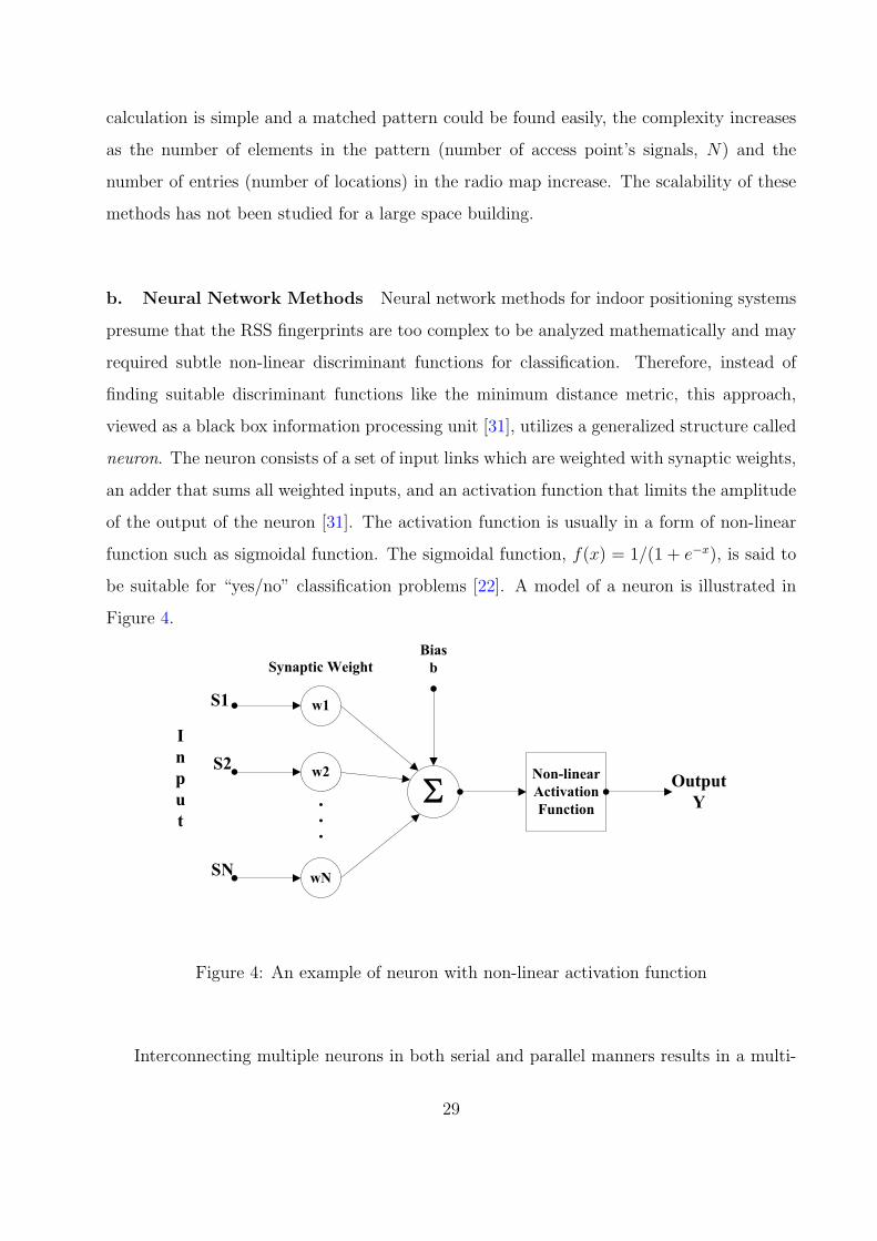
calculation is simple and a matched pattern could be found easily, the complexity increases
as the number of elements in the pattern (number of access point’s signals, N) and the
number of entries (number of locations) in the radio map increase. The scalability of these
methods has not been studied for a large space building.
b. Neural Network Methods Neural network methods for indoor positioning systems
presume that the RSS fingerprints are too complex to be analyzed mathematically and may
required subtle non-linear discriminant functions for classification. Therefore, instead of
finding suitable discriminant functions like the minimum distance metric, this approach,
viewed as a black box information processing unit [31], utilizes a generalized structure called
neuron. The neuron consists of a set of input links which are weighted with synaptic weights,
an adder that sums all weighted inputs, and an activation function that limits the amplitude
of the output of the neuron [31]. The activation function is usually in a form of non-linear
function such as sigmoidal function. The sigmoidal function, f(x) = 1/(1 + e−x), is said to
be suitable for “yes/no” classification problems [22]. A model of a neuron is illustrated in
Figure 4.
Figure 4: An example of neuron with non-linear activation function
Interconnecting multiple neurons in both serial and parallel manners results in a multi-
29
layer perceptron6 (MLP) neural network [22] in which signals travel sequentially from the
input layer to output layer and from the output of one neuron to the input of another
neuron. The layers in the middle between input and output layers are usually called hidden
layers. A simple feed-forward and fully connected neural network which consists of one
hidden layer was used to determine locations in [31]. The inputs consist of three features
each representing the RSS from three access points. The hidden layer is composed of 20
neurons and the output layer has 19 nodes corresponding to 19 positions on their map.
Battiti et al [40] also implemented a MLP neural network with one hidden layer that uses
the sigmoidal function and the output layer that uses an identity function (f(x) = x). The
final architecture used in [40] was 3→8→2 which refers to three inputs, eight hidden units
and two outputs of 2-D coordinates for 194 measurement points.
Each MLP neural network can be trained with samples of labeled location fingerprints in
order to iteratively calculate all synaptic weights inside the neurons. The training process is
interactive for each input sample of a location fingerprint in which the synaptic weights are
tuned so that the output is the correct position. A training technique called one-step-secant
(OSS) algorithm was used in [40] to iteratively adjust all synaptic weights with second-
derivative information. On the other hand, the error back-propagation algorithm is another
iterative algorithm that was used in [31] to find the synaptic weights. In a sense, these
training processes automatically create complex boundaries for location fingerprint classes.
As a flexible model, the MLP neural network requires no a priori knowledge of any
environment parameters such as the location of access point and building characteristics
(path loss exponent) [40]. The accuracy and the precision performance of [31, 40] was
reported to be better than nearest neighbor method, but not very significantly. For instance,
the results in [40] reported that the average error distance (accuracy performance) for MLP
neural network was 1.82 m while the average error distance for k-nearest neighbors was 1.81
m. The disadvantage of neural networks lies in their slow training time and may require
a large training set to get accurate location estimation. The problem of over-training or
over-fitting also occurred when the number of training iterations was larger than 3,000 and
6The perceptron is a type of artificial neural network invented by Frank Rosenblatt [39]. It consists ofone or more layers of artificial neurons.
30
resulted in poor location estimation performance [40]. Moreover, the error performance of
neural networks cannot be calculated analytically due to their complexity. Only measurement
test results can be done for data that was not in the training set.
Although neural network methods seem to be different from the statistical approach of the
nearest neighbor methods, the neural network methods have their equivalent counterparts in
statistical pattern recognition approach [37]. In other words, the neural networks also create
decision boundaries like nearest neighbor methods. For instance, a perceptron is similar
to a linear discriminant function and the multilayer perceptron methods are equivalent to
either non-linear discriminant analysis or a posteriori probability estimation [37]. Since the
neural networks avoid characterization of the statistics of the location fingerprints, they
rarely provide any insight information on the underlying mechanism of indoor positioning
systems.
c. Probabilistic Methods Instead of representing the location fingerprints with proto-
types or vectors of mean RSS as in the nearest neighbor approach, the probabilistic approach
models the location fingerprint with conditional probability and utilizes the Bayesian infer-
ence concept to estimate location [8, 23, 18]. This approach presumes a priori knowledge of
the probability distribution of the user’s location which is analytically shown to provide bet-
ter location accuracy than a deterministic approach as in the nearest neighbor methods [41].
The a priori location distribution allows the positioning system to maintain personalized
user location profiles as additional information [23] and can enhance the location tracking
application [8]. However, Battiti et al [22] point out that in order to create the conditional
probability this approach needs additional knowledge of the signal propagation model. The
knowledge could be in a form of empirical distributions of RSS at each location based on
measured training sets or in the form of a radio propagation model with estimated radio
parameters [22] without using any training set.
For each location coordinate L, we can estimate a conditional probability density func-
tion or the likelihood function P (F|L) from a training set consisting of samples of location
fingerprints and their labels. Roos et al [23] suggest two methods for estimating the like-
lihood function: the kernel method and the histogram method. Given n samples of RSS
31
from an access point at a location which is a one dimensional example, the kernel method
imposes a probability mass such as a Gaussian distribution on each sample of RSS values.
As a kernel function, each Gaussian distribution has a mean value ρ which equals to one of
n RSS samples and a proper standard deviation σ which is an arbitrary adjustable kernel
width. Then, the resulting likelihood function of a sample RSS s given a location L is an
equally weighted sum of all n Gaussian kernel functions:
P (s|L) =1
n
n∑i=1
[1√2πσ
exp
(−(s− ρ)2
2σ2
)]. (II.7)
From Equation II.7, the kernel width σ will have a smoothing effect on the probability
density estimation if its value is large. To extend this kernel method to multiple dimen-
sions or multiple access points, Roos et al make an independence assumption and multiply
all conditional probabilities together as P (F|L) = P (s1|L)P (s2|L) · · ·P (sN |L). They also
pointed out that the limiting case of a Gaussian kernel with kernel width approaching zero
is equivalent to the Euclidean nearest neighbor method [23].
On the other hand, the histogram method estimates the continuous density functions
by using discretized density functions. The histogram is essentially a fixed set of bins that
counts the frequency of occurrence of RSS samples that fall within a range of each bin. The
bin’s range is calculated from an adjustable number of bins and the known values of minimum
and maximum RSS values. Simple equal-width bins of 3, 7 and 27 were reported in [23].
The larger the number of bins, the better the histogram can approximate the probability
density function of RSS.
A slightly more sophisticated way to determine the P (F|L) is presented in [8] where
the authors calculate two different conditional probabilities from two different histograms
and multiply them together. The first conditional probability represents the frequency of
an access point’s observations given a location L. In other words, this probability indicates
how often the system can find the signal from that access point. The second conditional
probability represents the distribution of RSS from that access point given the same location.
Each location is assumed to have a priori probability P (L) which initially could be equally
likely for every location in set L. Then, the location estimation algorithms based on the
probabilistic approach apply the Bayes’ rule in order to find a posteriori distribution of that
32
location which is the conditional probability of the location L given the location fingerprint
F as:
P (L|F) =P (F|L)P (L)
P (F)=
P (F|L)P (L)∑k∈L P (F|Lk)P (Lk)
. (II.8)
According to Equation II.8, the probabilistic approach classifies the location fingerprints
according to the maximum estimated posterior probability; that is, it selects the location
fingerprint according the likelihood functions. For instance, in the case of two location
fingerprints, the Bayes decision rule will select position A (LA) over position B (LB) to
provide the smallest probability of error [38] when:
P (LA|F) > P (LB|F) (II.9)
P (F|LA)P (LA) > P (F|LB)P (LB). (II.10)
Since probabilistic methods have additional information on the location distribution,
they can provide better performance on location estimation. The disadvantages of this
model are that it may require a large training set to precisely estimate the conditional
probability distribution. Once again, these probabilistic methods require explicit knowledge
of the probability distributions of the location fingerprints. This emphasizes the need to
characterize of the WLAN’s received signal strength and the location fingerprints in greater
detail. Because the probabilistic methods incorporate some information of radio propagation,
they could provide insight on the underlying mechanism of indoor positioning.
d. Support Vector Machine Methods Recently, the support vector machines (SVMs)
technique was introduced as a non-parametric supervised classifier for approaching the indoor
positioning problem in [22]. The SVMs algorithm has its roots in statistical learning theory
introduced by Vapnik [42] in which it combines techniques of statistics, machine learning,
and neural networks together. To estimate the dependency between the RSS fingerprint
and the location from observations, this approach does not require detailed properties of the
dependency such as the propagation model as in the probabilistic method. The strength
of SVMs algorithm lies in its ability to generalize classification which minimizes the test
error or the classification error for the data after the training period. In other words, the
learning machine could be trained correctly by learning from a small training set and creating
33
sufficient structure for data classification without memorizing or over fitting the training
samples [22].
The fundamental concept of SVMs algorithm is based on the Structural Risk Minimiza-
tion (SRM) principle that tries to minimize the bound on an expected risk functional or
generalization error [22]. The risk functional is defined as an expected value of a loss func-
tion. The loss function is a measure of how much the function used to approximate the
pattern mapping differs from the real pattern mapping. The overall risk function is showed
to be bounded by the empirical risk function and Vapnik-Chervonenkis (VC) confidence
interval.
The problem of RSS fingerprint classification could be considered as a non-linear classifier
case. Here we explain the classification operation of SVMs without getting into too much of
the mathematical details. First, the vectors of location fingerprints are mapped into a higher
dimensional space called feature space [22] by using a function called kernel of the SVM to
perform vector transformation. There are a variety of SVMs kernel functions to choose from
such as polynomial functions, radial basis functions (RBF), Sigmoid kernel, and Analysis of
Variance (ANOVA) kernel [22]. Note that Battiti et al select a Radial Basis Function (RBF)
as the kernel of the SVM in [22]. Finally, the SVMs algorithm creates an optimal separating
hyperplane7 or decision surface in that feature space and uses the hyperplane to perform
classification. The separating hyperplane is not unique in general and is optimal when it has
a largest possible distance from the closest training point or a maximal margin. Support
vectors are the training vectors that are necessary to define the hyperplanes [22]; hence, the
support vector machine is the learning algorithm (machines) based on support vectors.
Although it is novel and the most sophisticated technique used successfully in the field
of pattern recognition, the performance of this technique for indoor positioning does not
differ very much from the other techniques. For the regression problem, it has comparable
performance to the weighted k nearest neighbors method. The result of error distance for
weighted k nearest neighbors was 3.93 m at 75% while the result error distance for SVMs
was 3.96 m at 75% in [22]. The SVMs algorithm is more suitable to solve classification
7“A hyperplane is any codimension-1 vector subspace of a vector space. Equivalently, a hyperplane Vin a vector space W is any subspace such that W/V is one-dimensional. Equivalently, a hyperplane is thelinear transformation kernel of any nonzero linear map from the vector space to the underlying field.” [43]
34
problems, i.e. to determine if the area is inside or outside a room [22]. The performance
of the positioning systems depends on acceptance error rather than the classification error
or mean square error in previous three methods [37]. To improve the classifier performance,
a proper kernel of the SVMs and its parameters must be selected appropriately since there
are several kernel functions to choose from. From the theoretical modeling perspective of
this study, the SVMs may be too complex to provide useful information on designing a
positioning system.
4. Summary of Existing Indoor Positioning Performance
This subsection briefly summarizes performance of existing indoor positioning system based
on location fingerprints and WLANs. The major performance metrics studied by all systems
are positioning accuracy which is a form of error measurement. As mentioned in Chapter I
and listed in Table 2, the accuracy of the location information is usually reported as an
error distance between the estimated location and the actual mobile location. However, the
report of accuracy should include the confidence interval or percentage of successful location
detection which is called the location precision. Recent research on positioning algorithms
has attracted a number of research groups to enhance these two performance with different
pattern recognition tools as discussed above. The system parameters of exiting systems are
summarized in Table 3 and the best reported performance of these systems are listed in
Table 4.
Table 3: Parameter comparison of indoor positioning systems
System Spacing Positions Samples/Pos. APs Orient. Env.RADAR [13] Nonuniform 70 80 ( 1
4 sec/samp.) 3 4 HallwaySaha et al [31] Min. 3.12m 19 1200 3 N/A 1-floorRoos et al [23] Uniform 2m 155 40 10 N/A 1-floorBattiti et at [22] N/A 257 N/A 6 N/A 1-floorLadd et al [8] 3m 11 1307 packets 5 2 HallwayPrasithsangaree et al [16] 1.5m, 3m 60 40 2-7 4 1-floorYoussef et al [18] 1.5m 110 300 4 N/A HallwayXiang et al [17] N/A 100 300 (2sec/samp.) 5 4 1-floor
Although the accuracy and the precision performance vary from one system to another
in Table 4, the differences among them are not very significant. It is easier to compare the
35
Table 4: Performance comparison of indoor positioning systems
System Algorithm Type Accuracy and PrecisionRADAR [13] Nearest Neighbor within 7 feet, 38%Saha et al [31] Nearest Neighbor & Neural Network no specified accuracy, 90%Roos et al [23] Bayesian best within 8.28 feet, 90%Battiti et at [22] SVMs, Bayesian, Neural Network all within 16-17 feet, 90%
& Weighted k Nearest NeighborLadd et al [8] Bayesian within 5 feet, 77%Prasithsangaree et al [16] Weighted k-Nearest Neighbor 25 feet at 75% & 40 feet at 95%Youssef et al [18] Bayesian within 7 feet, more than 90%Xiang et al [17] Bayesian with RSS distribution model within 6 feet, 90% (static device)
performance if one of these metrics is fixed, i.e. at the same precision, say 90% , the system
that reports smallest accuracy is the best. Note that these two performance metrics are
closely dependent. When we want to increase the accuracy (shorten deviated distance), the
precision performance has to be decreased (decrease the reliability percentage) [44]. On the
other hand, decreasing the accuracy (lengthen deviated distance) can increase the precision
performance (increase the reliability percentage). Interestingly, the results in [22] reported
a similar average accuracy performance within 3 m with all four positioning algorithms. It
is important to point out that each system has different parameter settings; therefore, com-
parison results summarized here may not be fair. Intuitively, we expect that a system that
has higher number of access points to perform better due to the higher dimension of the
location fingerprint vectors which result in better pattern separability. Moreover, a system
that has the positions only in the hallway may perform better because there are lesser num-
bers of positions in the system to be confused with. However, these two hypotheses were not
confirmed in the comparison above. These observations show a lack of unified performance
comparison methodology and a need for theoretical explanation of the relationship between
the indoor positioning performance and system parameters.
Besides these two performance metrics, other performance metrics which are delay, ca-
pacity, coverage, and scalability discussed in Section I.B are not considered by most of the
current studies. However, the computational complexity of the off-line or learning phase and
on-line or estimation phase of three positioning approaches (weighted k nearest neighbors,
36
Bayesian probabilistic approach, and multilayer preceptron neural network) are analyzed
by [22]. Concurrently, WLAN location determination via clustering and probability distri-
bution [18] is a study that tries to improve the positioning accuracy and reduces the com-
putational requirement in location estimation of positioning algorithms. Youssef et al [18]
proposed the Joint Clustering (JC) technique that uses clustering of locations sharing a com-
mon set of access points to reduce the computational complexity. However, their scheme is
still based on the probabilistic approach with Bayesian inference discussed above.
Unrelated to the previous discussion on pattern recognition, sensor fusion techniques
allow the positioning system to exploit redundancies and contradictions to reduce overall
location uncertainty [24]. This technique helps improve accuracy and precision of positioning
systems. An example is presented in [8] where the system combines multiple independent
observations to gain a better estimate from the positioning algorithm. A Hidden Markov
Model (HMM), which is used in [8] to track the user, increases the accuracy and the precision
performance. Utilizing only one of the location sensing techniques usually yields limited
system performance and high uncertainty of location information. The hybrid approach,
which consists of two or more sensing techniques and technologies, can also improve the
accuracy and the precision performance of indoor positioning systems. An example of a
hybrid system is discussed in [5] when AOA and TDOA are combined.
E. CONCLUSIONS
Although there are research studies that report on the time series of WLAN received signal
strength [13, 32, 31] and the unique dependency of signal strength and location for indoor
positioning system, there are surprisingly no studies of the pattern of location fingerprint.
Few properties are known of the location fingerprint such as its distribution even though
they are necessary for pattern classification. Two research groups tried to point out the
distribution of RSS, but their results were contradictory. One group suggested a lognormally
distributed RSS while another showed asymmetric distributions with multi-modal properties.
However, their environments were different. This study investigates the pattern of received
37
signal strength or the location fingerprint in greater detail as a part of the contribution.
On the improvement of performance of positioning systems, the research community has
been emphasizing the machine learning approach such as neural networks and support vector
machines. However, these two approaches are quite complex and require careful selection
of learning machine parameters. Since both neural networks and support vector machines
are non-parametric classifiers [45], they do not assume any knowledge of the distributions
of the location fingerprints. Both approaches are considered as black boxes that cannot
provide insight on how to improve the positioning systems beyond the complexity of their
generic learning machines. Thus, this study limits the scope of study to the nearest neighbor
and probabilistic approaches. The nearest neighbor is the simplest non-parametric classifier
that can be analyzed while the probabilistic approach is a parametric classifier that assume
some knowledge of the distribution of the location fingerprints. For instance, the Euclidean
distance technique implicitly assumes that classified patterns are Gaussian with symmetric
variance on each element in the patterns. On the other hand, the probabilistic approach
intrinsically maintains distributions of the location fingerprints via either histogram or para-
metric estimation.
The design of indoor positioning systems requires an analytical model that can explain
the relationship between the system performance and system parameters. The adoption of
location-based services in the future will require an efficient and effective design methodology
for indoor positioning systems. The design area of indoor positioning has not been consid-
ered at all in any literature. There is no simple way to predict the performance of indoor
positioning without actually performing a real measurement to test the positioning algorithm.
Therefore, this study proposes a model of location fingerprints which can be incorporated
into an analytical model for study of indoor positioning systems.
Depending on the positioning algorithm, the impact of database searching performance
should also be investigated. This aspect is not emphasized very much among the existing
positioning system studies. In particularly, the nearest neighbor methods can become inef-
ficient when the number of positions in radio map becomes huge for large sized buildings.
This issue influences the complexity and scalability performance of the indoor positioning
system.
38

Finally, there is still a lack of a standard framework for comparing different positioning
systems in the community [23]. Some did provide the precision in percentages while others
only report the average accuracy in meters. The minimum distance separation, the number of
positions, and coverage area from different papers are also different and makes the comparison
among them difficult.
39
III. PROPERTIES OF RECEIVED SIGNAL STRENGTH
As described previously, initial data analysis is extremely important for location fingerprint-
ing. In this chapter, we investigate the properties of the received signal strength (RSS) values
as reported by IEEE 802.11b wireless network interface cards (NICs). This analysis of the
RSS values is needed to understand the underlying features of location-dependent RSS pat-
terns and location fingerprints. Although there is extensive knowledge available regarding
radio frequency (RF) phenomena and properties of the received signal in indoor environ-
ments (such as the distance dependence property [46]), such knowledge is aimed towards
other applications, in particular communications capability and receiver design, making it
limited for positioning applications. An understanding of the properties of the RSS values
for location fingerprinting can assist in improving the design of positioning algorithms and in
deployment of indoor positioning systems. A set of mathematical assumptions is proposed
at the end of this chapter based on the results of this analyses. These assumptions will be
used in the later chapters for developing models and providing deployment guidelines.
A. MEASUREMENT SETUP
An IBM A22m laptop computer equipped with a Lucent Orinoco WLAN card and a client
manager software were primarily used to collect samples of RSS from access points (APs)
at the University of Pittsburgh. The WLAN card is plugged into a PCMCIA slot on the
right side of the laptop. The client manager software is a site-survey tool from Lucent [47]
which provides link quality and AP monitoring capabilities. This software monitors IEEE
802.11b radio frequency channels which operate in the 2.4 GHz band. Note that this radio
40
spectrum is shared by other equipment in the industrial, scientific, and medical (ISM) band
such as Bluetooth. The number of non-overlapping channels for IEEE 802.11b is three [48]
and they are re-used when more than three access points are needed in any area. The
information available to the user from the client manager software includes the AP’s name,
AP’s medium access control (MAC) address, received signal (dBm), noise (dBm), signal-to-
noise ratio (SNR in dB) and channel number.
The measurement reported in subsequent sections is done by taking logs of RSS measure-
ments from APs “visible” to a mobile client over a certain period of time. For a particular
location, vectors of RSS are formed based on measurable signals from APs during the mea-
surement time. This study assumes that the client manager software provides the same
information as a query from a positioning software accessing a network interface card. The
RSS values reported by most WLAN cards are in integral steps of 1 dBm. Note that all
possible RSS values cannot be represented by a set of integer values [49]. The received signal
sensitivity of a particular make of WLAN card limits the measurable range of the RSS. For
instance, a Lucent Orinoco WLAN card has its receiver sensitivity between -93 dBm and 0
dBm [47]. The smallest signal value that most standard 802.11 cards can receive and report
corresponds to around -96 dBm [49]. The highest typical value of the RSS found in our
experiment using Lucent’s Orinoco card is approximately -30 dBm at one meter from any
AP. According to [49], the maximum signal level reported by most standard 802.11 cards is
-10 dBm even though the actual received signal strength can be higher.
Because the client manager software is proprietary for the Lucent Orinoco card, measure-
ment experiments using this software implies limited control over the setting of the sampling
period and choice of WLAN cards. To obtain the RSS for different wireless network cards,
in this study we used a small program that captures RSS data based on available example
code from Microsoft’s Windows XP driver development kit (DDK) [50] and the University
of California at San Diego’s Wireless Research API (WRAPI) [51]. The program utilizes
Windows XP’s Network Device Interface Specification (NDIS) version 5.1. It is a kernel
layer standard API which defines the interface between the network interface card and the
medium access control (MAC) protocol driver. A WIN32 API called DeviceIoControl allows
any user’s application to query Microsoft’s object identifier (OID) such as OID 802 11 RSSI
41
to obtain received signal strength indication (RSSI) on a wireless network card. The RSSI
returned by Windows’s miniport driver is measured in dBm and has typical values between
-10 and -200 [52].
1. Experimental Design
Different factors that affect the indoor RSS are the user’s presence/absence, his/her orien-
tation, time of day, building types and material, distance from transmitter, and make of
wireless cards. These factors are considered because they certainly affect the WLAN’s RSS
as shown in this chapter. These factors are by no means exhaustive. Other possible factors
are antenna orientation, directionality and type but they are not considered here (we only
consider omnidirectional antennas). A number of experiments that vary these different fac-
tors are performed and the results are analyzed to identify the statistical properties of RSS
patterns. The results are applied to model indoor location fingerprints in the next chapter.
Table 5 lists two groups of the factors and the options used in the subsequent studies.
The groups are divided according to the factors’ effects. Note that this study performs
measurements using a quasi-static laptop only. While we are aware of the effect of WLAN’s
mobility it is beyond the scope of current study. Our assumption here is that typical usage
of WLANs occurs under stationary conditions. The movement of the mobile station causes
fluctuation of the received signal strength which is called small-scale fading [12]. Larger
fluctuations of RSS values has been exploited to infer the movement of the mobile station
in [53].
The first factor (proximity of user to mobile) is considered because there are different
location-services applications that may or may not cater to a human user. When a user is
equipped with a mobile terminal and faces different directions, the study in [13] reports that
different user orientations can cause a change in the location fingerprint at the same location.
Our study confirms this observation through the second factor. The third factor considers
the make of wireless cards which could have different chipsets and hardware implementation.
Some vendors have a better hardware design than others.
Because of changes in environment over time (such as movement and number of people)
42
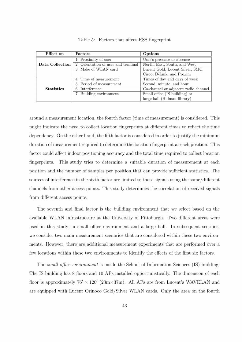
Table 5: Factors that affect RSS fingerprint
Effect on Factors Options1. Proximity of user User’s presence or absence
Data Collection 2. Orientation of user and terminal North, East, South, and West3. Make of WLAN card Lucent Gold, Lucent Silver, SMC,
Cisco, D-Link, and Proxim4. Time of measurement Times of day and days of week5. Period of measurement Second, minute, and hour
Statistics 6. Interference Co-channel or adjacent radio channel7. Building environment Small office (IS building) or
large hall (Hillman library)
around a measurement location, the fourth factor (time of measurement) is considered. This
might indicate the need to collect location fingerprints at different times to reflect the time
dependency. On the other hand, the fifth factor is considered in order to justify the minimum
duration of measurement required to determine the location fingerprint at each position. This
factor could affect indoor positioning accuracy and the total time required to collect location
fingerprints. This study tries to determine a suitable duration of measurement at each
position and the number of samples per position that can provide sufficient statistics. The
sources of interference in the sixth factor are limited to those signals using the same/different
channels from other access points. This study determines the correlation of received signals
from different access points.
The seventh and final factor is the building environment that we select based on the
available WLAN infrastructure at the University of Pittsburgh. Two different areas were
used in this study: a small office environment and a large hall. In subsequent sections,
we consider two main measurement scenarios that are considered within these two environ-
ments. However, there are additional measurement experiments that are performed over a
few locations within these two environments to identify the effects of the first six factors.
The small office environment is inside the School of Information Sciences (IS) building.
The IS building has 8 floors and 10 APs installed opportunistically. The dimension of each
floor is approximately 76′ × 120′ (23m×37m). All APs are from Lucent’s WAVELAN and
are equipped with Lucent Orinoco Gold/Silver WLAN cards. Only the area on the fourth
43
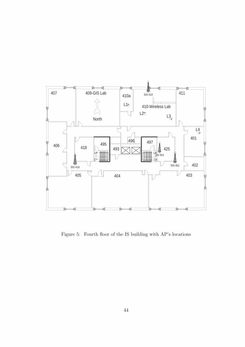
UP
DN
UP
DN
405 404 403
402
406
407
401
411
425 418 493
496 495 497
409-GIS Lab
410-Wireless Lab
410a
L1
L2
SIS 410
SIS 418 SIS 401
SIS 501
North
z
z
z
z
L3
L4
Figure 5: Fourth floor of the IS building with AP’s locations
44
floor is used for this experiment. Locations of access points that have strong signals on the
fourth floor are shown in Figure 5. The operating frequencies and the last sixteen bits of the
MAC addresses of these access points are listed in Table 6. Note that SIS501 AP is located
on the fifth floor and no AP is located on the third floor.
Table 6: Measurable access points on 4th floor in Information Science building
Access Point Name Location Frequency Channel MAC AddressSIS401 Fourth Floor 11 xxxxxxxxE6F7SIS410 Fourth Floor 6 xxxxxxxx886BSIS418 Fourth Floor 1 xxxxxxxxE6E8SIS501 Fifth Floor 6 xxxxxxxxE6EE
For the measurement of the small office environment, we defined a small area as a grid
of 25 locations where 20 of them were placed inside the room 410 and five of them were
placed along the corridor as shown by dots in Fig. 6. The minimum distance between two
locations or grid spacing was fixed at one meter because RSS patterns could overlap more
than a larger distance. Location fingerprints were collected at each location for a period of
five minutes at a rate of four samples per second. This resulted in 25 points × 3 APs = 75
RSS distributions. The user’s orientation was limited to the north direction only.
The large hall environment is inside the Hillman library building. This building has
five floors including a ground floor. The dimension of each floor is approximately 197′ ×197′ (60m×60m). APs are installed to provide wireless access to students who use the
library. There are six APs located throughout the building and all APs are from Enterasys’s
RoamAbout. There are two APs each on the ground floor, the second floor, and the fourth
floor. The APs placed on different floors are marked in Figure 7 of the first floor. The
building is divided into two wings with three elevators and two stairways in the center of the
building as showed in Figure 7. Two additional stairwells are located near the center-edge
of each wing.
All measurements were done inside the area of the first floor where there is a large open
space (denoted by dashed lines) that shares the ceiling with the second floor. Figure 7 also
shows the locations of measurement with small arrows. Signals from all six AP’s can be
detected on this floor, but their coverage is not complete throughout the floor. The access
45
UPDN UPDN405 404 403402406407
401411
425418 493 496495 497409-GIS Lab 410-Wireless LabSIS410
SIS418 SIS501 SIS401North
Figure 6: Location of access points on the 4th floor of IS building
46
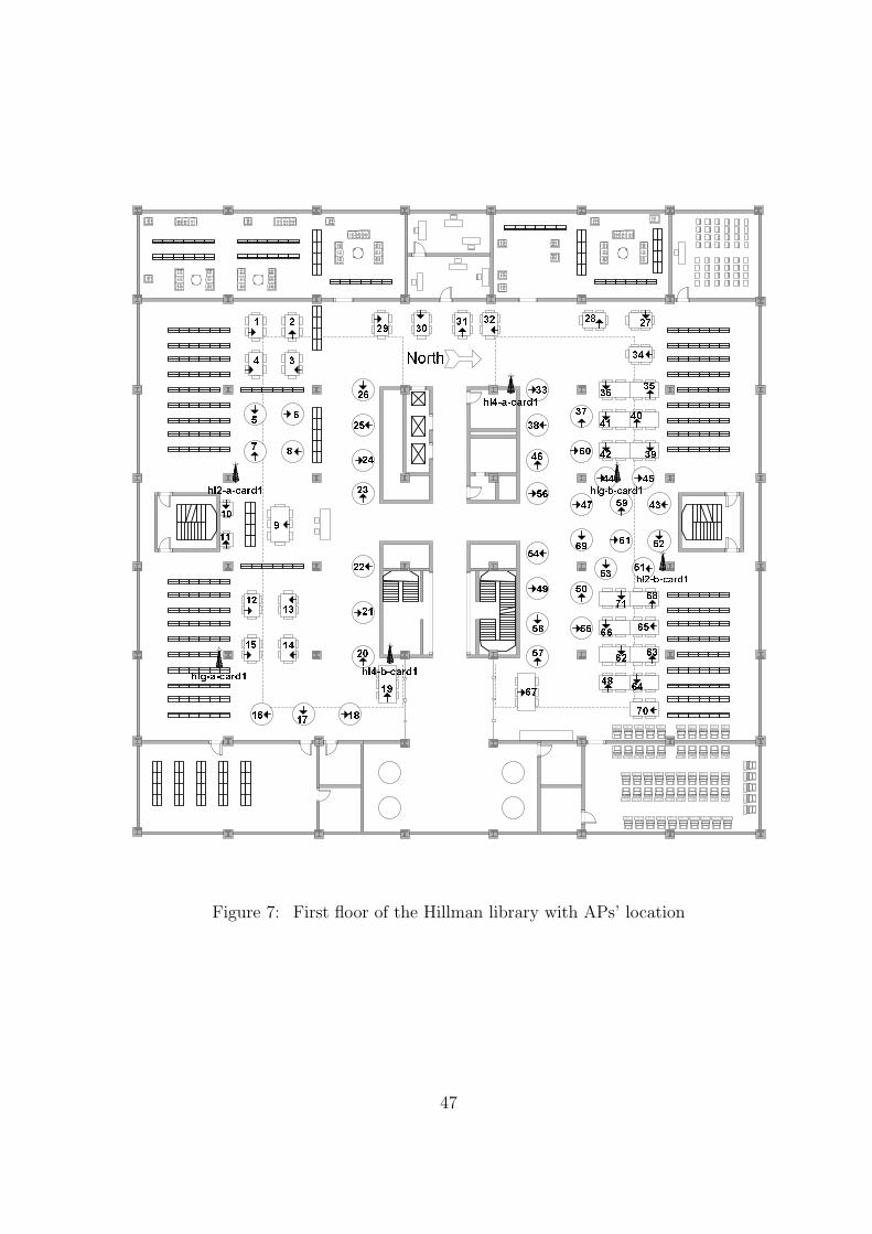
North hl4-a-card1hl4-b-card1hlg-a-card1
hlg-b-card1hl2-b-card1hl2-a-card11 2345 67 891011 12 13141516 17 18 1920212223242526 29 30 31 32 272833 3435363738 39404142 4344 4546 6160
4849 50 51 525354 55565758 5969 62 6364656667 687047 71
Figure 7: First floor of the Hillman library with APs’ location
47
point names and their corresponding operating frequencies are summarized in Table 7.
Table 7: Access points in Hillman library
Access Point Name Location Frequency Channel MAC Addresshlg-a-card1 Ground Floor 1 xxxxxxxxF261hlg-b-card1 Ground Floor 11 xxxxxxxxF616hl2-a-card1 Second Floor 11 xxxxxxxxF618hl2-b-card1 Second Floor 6 xxxxxxxx4115hl4-a-card1 Fourth Floor 1 xxxxxxxxF5FChl4-b-card1 Fourth Floor 6 xxxxxxxxF23E
Table 8: Experimental design and measurement factors
Factors Scenario 1 Scenario 2Building Type 4th Fl. IS building 1st Fl. Hillman Library
Proximity of Laptop User Presence PresenceUser and Terminal Orientation North only Dependent on location
Time of Measurement Afternoon to evening Afternoon to eveningSpan of Measurement 1 day 32 days
Period of Measurement per Location 5 minutes 1 hourSampling Period 0.25 second 1 second
Number of Locations 25 71Distance between Locations Uniform 1 meter Non-uniform, 2 meters or more
Client Card Vendor Lucent Orinoco Gold Lucent Orinoco GoldAccess Point Vendor Lucent WAVELAN Enterasys RoamAbout
Software Tool Lucent client manager Lucent client manager
Based on the two environments described above, Table 8 summarizes the measurement
scenarios used to collect most of the RSS data used in subsequent analyses. Both scenarios
have a user operating the laptop during all period of measurement. Because of limited control
over the client manager software, the number of data points collected at each location vary
from one location to another. Note that the distance between different locations in Scenario
2 varied according to locations of reading tables inside the library. The measurement in
Scenario 2 is performed over a period of one hour causing a large span of measurement over
several days due to the three-hour limitation of the laptop’s battery.
According to Table 5, we group the factors studied into those that affect the data collec-
tion and those that affect the statistics of the RSS. The organization in the next two sections
will follow these two categories. Section III.B investigates the first three factors in Table 5
48
that cause changes to the received signal strength and its average value. These factors should
be taken into account when collecting location fingerprints. The rest of the factors will be
discussed along with statistical properties of the RSS in Section III.C.
B. COLLECTING MEASUREMENT OF RECEIVED SIGNAL STRENGTH
1. User’s Effect
For indoor positioning systems based on a WLAN infrastructure, users typically carry laptops
or work near devices equipped with WLAN interface cards. The effect of the user’s presence
close to WLAN antennas plays an important role on the mean and the spread of RSS values
(variance). An observation was made in [13] that the user’s orientation can cause a variation
in RSS level up to 5 dBm. However, no analysis of the data was provided nor were there
measurements when no user is present during the measurement.
a. User’s Body To study the effect of the user’s body, we performed measurement of
the signal from SIS410 at location L1 inside the room IS 410a in Figure 5. The distance
between the transmitter (AP) and the receiver (MS) is approximately 7m and the MS does
not have a clear line-of-sight to the AP. The data were recorded for two hours. During the
first hour, the user was present, while no user was present in the second hour. The results
are shown as plots of histograms from both hours in Figure 8.
Figure 8-a and 8-b depict the difference between two histograms at the same measurement
position. The user’s body influences the RSS distribution by spreading the range of RSS
values by a significant amount. The standard deviation is reduced from approximately 3.00
dBm to 0.68 dBm when the user is absent. An explanation of this effect is that the user is
acting like a reflector or scatterer of the signal and causes the received signal to fluctuate
more than otherwise. The mean increases from -71.6 dBm to -70.4 dBm without the user’s
body. Clearly, it is essential to collect data based on the type of location application. When
a positioning system is supposed to cater to real users, it is essential to have a user present
49
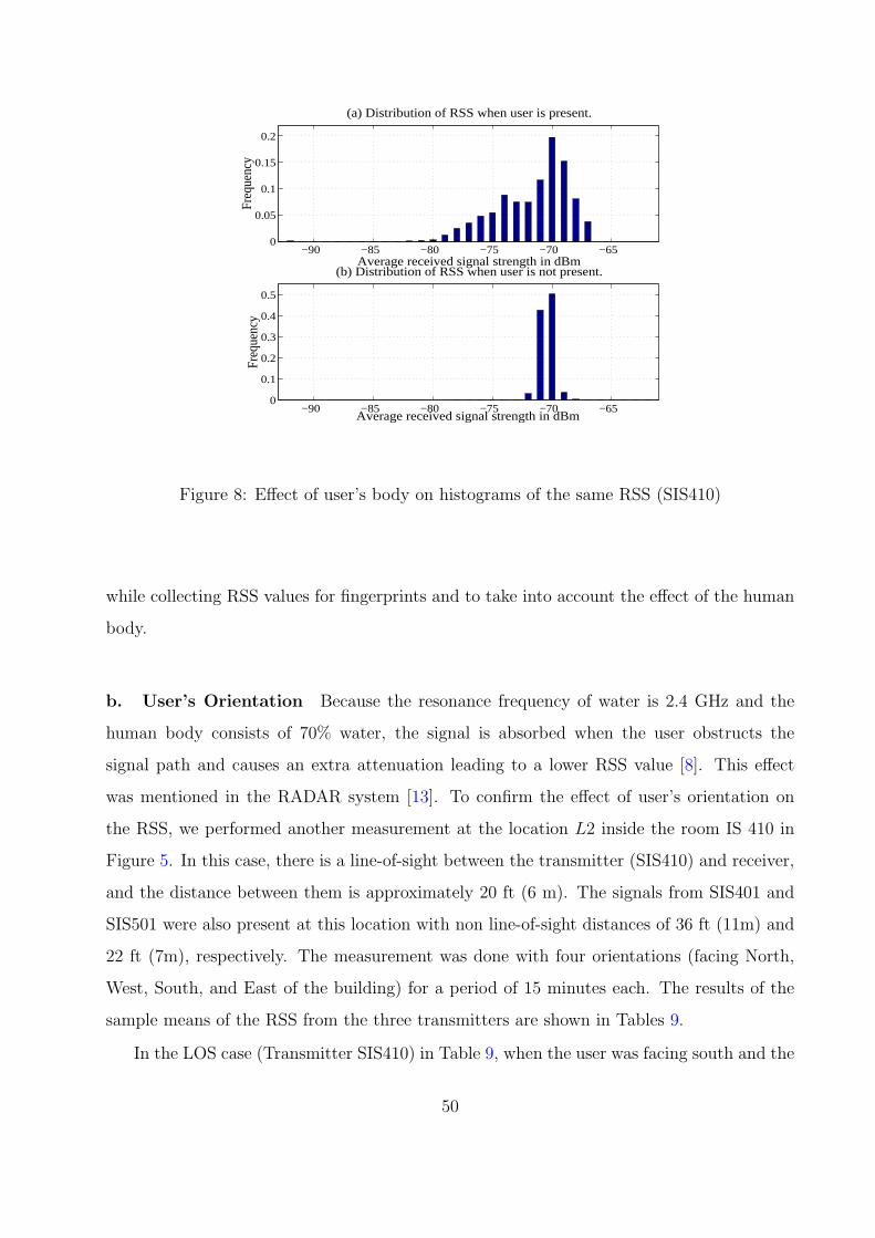
−90 −85 −80 −75 −70 −650
0.05
0.1
0.15
0.2
Average received signal strength in dBmF
requ
ency
(a) Distribution of RSS when user is present.
−90 −85 −80 −75 −70 −650
0.1
0.2
0.3
0.4
0.5
Average received signal strength in dBm
Fre
quen
cy
(b) Distribution of RSS when user is not present.
Figure 8: Effect of user’s body on histograms of the same RSS (SIS410)
while collecting RSS values for fingerprints and to take into account the effect of the human
body.
b. User’s Orientation Because the resonance frequency of water is 2.4 GHz and the
human body consists of 70% water, the signal is absorbed when the user obstructs the
signal path and causes an extra attenuation leading to a lower RSS value [8]. This effect
was mentioned in the RADAR system [13]. To confirm the effect of user’s orientation on
the RSS, we performed another measurement at the location L2 inside the room IS 410 in
Figure 5. In this case, there is a line-of-sight between the transmitter (SIS410) and receiver,
and the distance between them is approximately 20 ft (6 m). The signals from SIS401 and
SIS501 were also present at this location with non line-of-sight distances of 36 ft (11m) and
22 ft (7m), respectively. The measurement was done with four orientations (facing North,
West, South, and East of the building) for a period of 15 minutes each. The results of the
sample means of the RSS from the three transmitters are shown in Tables 9.
In the LOS case (Transmitter SIS410) in Table 9, when the user was facing south and the
50
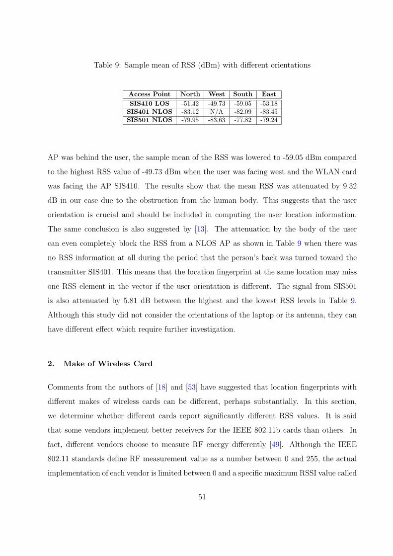
Table 9: Sample mean of RSS (dBm) with different orientations
Access Point North West South EastSIS410 LOS -51.42 -49.73 -59.05 -53.18
SIS401 NLOS -83.12 N/A -82.09 -83.45SIS501 NLOS -79.95 -83.63 -77.82 -79.24
AP was behind the user, the sample mean of the RSS was lowered to -59.05 dBm compared
to the highest RSS value of -49.73 dBm when the user was facing west and the WLAN card
was facing the AP SIS410. The results show that the mean RSS was attenuated by 9.32
dB in our case due to the obstruction from the human body. This suggests that the user
orientation is crucial and should be included in computing the user location information.
The same conclusion is also suggested by [13]. The attenuation by the body of the user
can even completely block the RSS from a NLOS AP as shown in Table 9 when there was
no RSS information at all during the period that the person’s back was turned toward the
transmitter SIS401. This means that the location fingerprint at the same location may miss
one RSS element in the vector if the user orientation is different. The signal from SIS501
is also attenuated by 5.81 dB between the highest and the lowest RSS levels in Table 9.
Although this study did not consider the orientations of the laptop or its antenna, they can
have different effect which require further investigation.
2. Make of Wireless Card
Comments from the authors of [18] and [53] have suggested that location fingerprints with
different makes of wireless cards can be different, perhaps substantially. In this section,
we determine whether different cards report significantly different RSS values. It is said
that some vendors implement better receivers for the IEEE 802.11b cards than others. In
fact, different vendors choose to measure RF energy differently [49]. Although the IEEE
802.11 standards define RF measurement value as a number between 0 and 255, the actual
implementation of each vendor is limited between 0 and a specific maximum RSSI value called
51
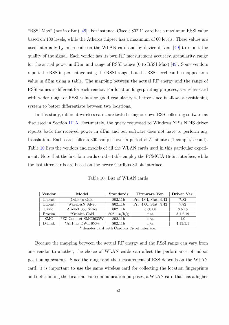
“RSSI Max” (not in dBm) [49]. For instance, Cisco’s 802.11 card has a maximum RSSI value
based on 100 levels, while the Atheros chipset has a maximum of 60 levels. These values are
used internally by microcode on the WLAN card and by device drivers [49] to report the
quality of the signal. Each vendor has its own RF measurement accuracy, granularity, range
for the actual power in dBm, and range of RSSI values (0 to RSSI Max) [49]. Some vendors
report the RSS in percentage using the RSSI range, but the RSSI level can be mapped to a
value in dBm using a table. The mapping between the actual RF energy and the range of
RSSI values is different for each vendor. For location fingerprinting purposes, a wireless card
with wider range of RSSI values or good granularity is better since it allows a positioning
system to better differentiate between two locations.
In this study, different wireless cards are tested using our own RSS collecting software as
discussed in Section III.A. Fortunately, the query requested to Windows XP’s NDIS driver
reports back the received power in dBm and our software does not have to perform any
translation. Each card collects 300 samples over a period of 5 minutes (1 sample/second).
Table 10 lists the vendors and models of all the WLAN cards used in this particular experi-
ment. Note that the first four cards on the table employ the PCMCIA 16-bit interface, while
the last three cards are based on the newer Cardbus 32-bit interface.
Table 10: List of WLAN cards
Vendor Model Standards Firmware Ver. Driver Ver.Lucent Orinoco Gold 802.11b Pri. 4.04, Stat. 9.42 7.82Lucent WaveLAN Silver 802.11b Pri. 4.00, Stat. 9.42 7.82Cisco Aironet 350 Series 802.11b 5.60.08 8.6.16
Proxim *Orinico Gold 802.11a/b/g n/a 3.1.2.19SMC *EZ Connect SMC2635W 802.11b n/a 1.0
D-Link *AirPlus DWL-650+ 802.11b n/a 4.15.5.1* denotes card with Cardbus 32-bit interface.
Because the mapping between the actual RF energy and the RSSI range can vary from
one vendor to another, the choice of WLAN cards can affect the performance of indoor
positioning systems. Since the range and the measurement of RSS depends on the WLAN
card, it is important to use the same wireless card for collecting the location fingerprints
and determining the location. For communication purposes, a WLAN card that has a higher
52
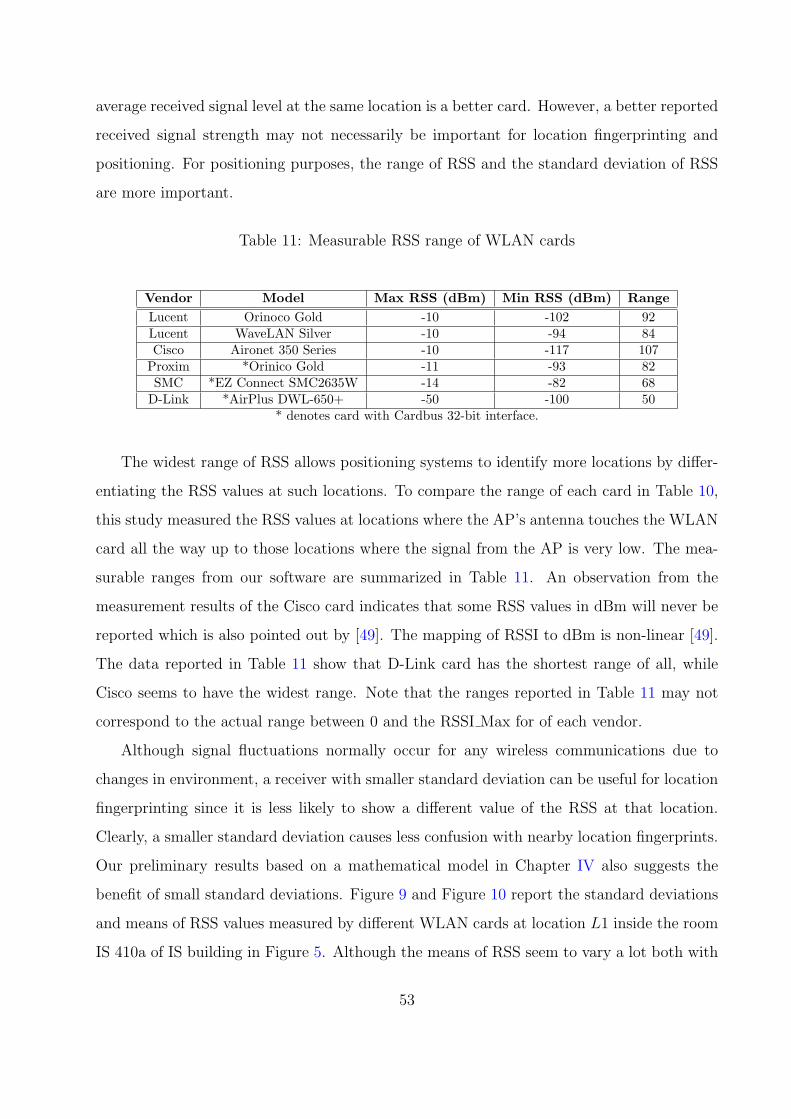
average received signal level at the same location is a better card. However, a better reported
received signal strength may not necessarily be important for location fingerprinting and
positioning. For positioning purposes, the range of RSS and the standard deviation of RSS
are more important.
Table 11: Measurable RSS range of WLAN cards
Vendor Model Max RSS (dBm) Min RSS (dBm) RangeLucent Orinoco Gold -10 -102 92Lucent WaveLAN Silver -10 -94 84Cisco Aironet 350 Series -10 -117 107
Proxim *Orinico Gold -11 -93 82SMC *EZ Connect SMC2635W -14 -82 68
D-Link *AirPlus DWL-650+ -50 -100 50* denotes card with Cardbus 32-bit interface.
The widest range of RSS allows positioning systems to identify more locations by differ-
entiating the RSS values at such locations. To compare the range of each card in Table 10,
this study measured the RSS values at locations where the AP’s antenna touches the WLAN
card all the way up to those locations where the signal from the AP is very low. The mea-
surable ranges from our software are summarized in Table 11. An observation from the
measurement results of the Cisco card indicates that some RSS values in dBm will never be
reported which is also pointed out by [49]. The mapping of RSSI to dBm is non-linear [49].
The data reported in Table 11 show that D-Link card has the shortest range of all, while
Cisco seems to have the widest range. Note that the ranges reported in Table 11 may not
correspond to the actual range between 0 and the RSSI Max for of each vendor.
Although signal fluctuations normally occur for any wireless communications due to
changes in environment, a receiver with smaller standard deviation can be useful for location
fingerprinting since it is less likely to show a different value of the RSS at that location.
Clearly, a smaller standard deviation causes less confusion with nearby location fingerprints.
Our preliminary results based on a mathematical model in Chapter IV also suggests the
benefit of small standard deviations. Figure 9 and Figure 10 report the standard deviations
and means of RSS values measured by different WLAN cards at location L1 inside the room
IS 410a of IS building in Figure 5. Although the means of RSS seem to vary a lot both with
53
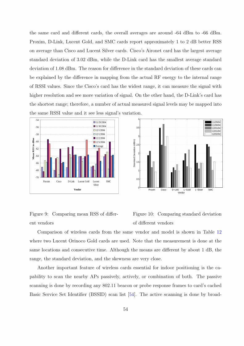
the same card and different cards, the overall averages are around -64 dBm to -66 dBm.
Proxim, D-Link, Lucent Gold, and SMC cards report approximately 1 to 2 dB better RSS
on average than Cisco and Lucent Silver cards. Cisco’s Aironet card has the largest average
standard deviation of 3.02 dBm, while the D-Link card has the smallest average standard
deviation of 1.08 dBm. The reason for difference in the standard deviation of these cards can
be explained by the difference in mapping from the actual RF energy to the internal range
of RSSI values. Since the Cisco’s card has the widest range, it can measure the signal with
higher resolution and see more variation of signal. On the other hand, the D-Link’s card has
the shortest range; therefore, a number of actual measured signal levels may be mapped into
the same RSSI value and it see less signal’s variation.
-70
-68
-66
-64
-62
-60
-58
-56
-54
Proxim Cisco D-Link Lucent Gold LucentSilver
SMC
Vendor
Mea
n R
SS
in
dB
m
11/29/2004
11/30/2004
12/1/2004
12/1/2004
12/2/2004
12/5/2004
Average
Figure 9: Comparing mean RSS of differ-
ent vendors
Proxim Cisco D−Link L−Gold L−Silver SMC0
0.5
1
1.5
2
2.5
3
3.5
4
Vendor
Sta
nd
ard
De
via
tion
(d
Bm
)
11/29/0411/30/0412/01/0412/01/0412/02/04
Figure 10: Comparing standard deviation
of different vendors
Comparison of wireless cards from the same vendor and model is shown in Table 12
where two Lucent Orinoco Gold cards are used. Note that the measurement is done at the
same locations and consecutive time. Although the means are different by about 1 dB, the
range, the standard deviation, and the skewness are very close.
Another important feature of wireless cards essential for indoor positioning is the ca-
pability to scan the nearby APs passively, actively, or combination of both. The passive
scanning is done by recording any 802.11 beacon or probe response frames to card’s cached
Basic Service Set Identifier (BSSID) scan list [54]. The active scanning is done by broad-
54
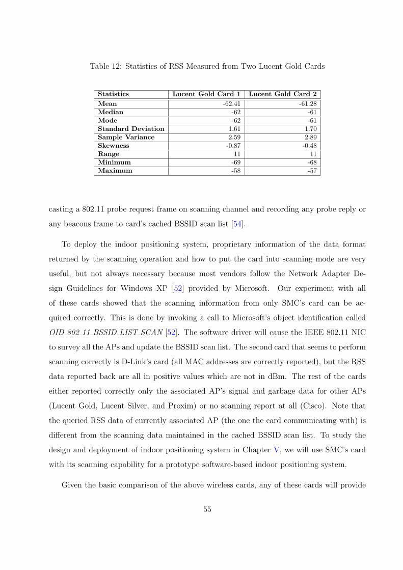
Table 12: Statistics of RSS Measured from Two Lucent Gold Cards
Statistics Lucent Gold Card 1 Lucent Gold Card 2Mean -62.41 -61.28Median -62 -61Mode -62 -61Standard Deviation 1.61 1.70Sample Variance 2.59 2.89Skewness -0.87 -0.48Range 11 11Minimum -69 -68Maximum -58 -57
casting a 802.11 probe request frame on scanning channel and recording any probe reply or
any beacons frame to card’s cached BSSID scan list [54].
To deploy the indoor positioning system, proprietary information of the data format
returned by the scanning operation and how to put the card into scanning mode are very
useful, but not always necessary because most vendors follow the Network Adapter De-
sign Guidelines for Windows XP [52] provided by Microsoft. Our experiment with all
of these cards showed that the scanning information from only SMC’s card can be ac-
quired correctly. This is done by invoking a call to Microsoft’s object identification called
OID 802 11 BSSID LIST SCAN [52]. The software driver will cause the IEEE 802.11 NIC
to survey all the APs and update the BSSID scan list. The second card that seems to perform
scanning correctly is D-Link’s card (all MAC addresses are correctly reported), but the RSS
data reported back are all in positive values which are not in dBm. The rest of the cards
either reported correctly only the associated AP’s signal and garbage data for other APs
(Lucent Gold, Lucent Silver, and Proxim) or no scanning report at all (Cisco). Note that
the queried RSS data of currently associated AP (the one the card communicating with) is
different from the scanning data maintained in the cached BSSID scan list. To study the
design and deployment of indoor positioning system in Chapter V, we will use SMC’s card
with its scanning capability for a prototype software-based indoor positioning system.
Given the basic comparison of the above wireless cards, any of these cards will provide
55
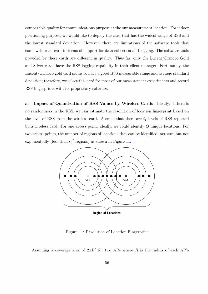
comparable quality for communications purpose at the our measurement location. For indoor
positioning purpose, we would like to deploy the card that has the widest range of RSS and
the lowest standard deviation. However, there are limitations of the software tools that
come with each card in terms of support for data collection and logging. The software tools
provided by these cards are different in quality. Thus far, only the Lucent/Orinoco Gold
and Silver cards have the RSS logging capability in their client manager. Fortunately, the
Lucent/Orinoco gold card seems to have a good RSS measurable range and average standard
deviation; therefore, we select this card for most of our measurement experiments and record
RSS fingerprints with its proprietary software.
a. Impact of Quantization of RSS Values by Wireless Cards Ideally, if there is
no randomness in the RSS, we can estimate the resolution of location fingerprint based on
the level of RSS from the wireless card. Assume that there are Q levels of RSS reported
by a wireless card. For one access point, ideally, we could identify Q unique locations. For
two access points, the number of regions of locations that can be identified increases but not
exponentially (less than Q2 regions) as shown in Figure 11.
AP1 AP2
Region of Locations
Figure 11: Resolution of Location Fingerprint
Assuming a coverage area of 2πR2 for two APs where R is the radius of each AP’s
56
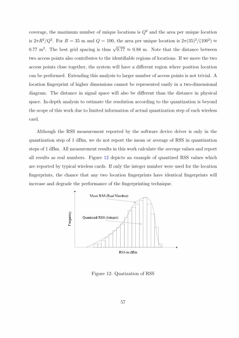
coverage, the maximum number of unique locations is Q2 and the area per unique location
is 2πR2/Q2. For R = 35 m and Q = 100, the area per unique location is 2π(35)2/(1002) ≈0.77 m2. The best grid spacing is thus
√0.77 ≈ 0.88 m. Note that the distance between
two access points also contributes to the identifiable regions of locations. If we move the two
access points close together, the system will have a different region where position location
can be performed. Extending this analysis to larger number of access points is not trivial. A
location fingerprint of higher dimensions cannot be represented easily in a two-dimensional
diagram. The distance in signal space will also be different than the distance in physical
space. In-depth analysis to estimate the resolution according to the quantization is beyond
the scope of this work due to limited information of actual quantization step of each wireless
card.
Although the RSS measurement reported by the software device driver is only in the
quantization step of 1 dBm, we do not report the mean or average of RSS in quantization
steps of 1 dBm. All measurement results in this work calculate the average values and report
all results as real numbers. Figure 12 depicts an example of quantized RSS values which
are reported by typical wireless cards. If only the integer number were used for the location
fingerprints, the chance that any two location fingerprints have identical fingerprints will
increase and degrade the performance of the fingerprinting technique.Mean RSS (Real Number)Quantized RSS (Integer) RSS in dBmFrequencyFigure 12: Quatization of RSS
57
C. STATISTICAL PROPERTIES OF RECEIVED SIGNAL STRENGTH
Changes to the signal due to propagation indoors is difficult to predict because of the dense
environment and propagation effects such as reflection, diffraction, and scattering [46]. The
multipath fading effect, which is the result of either constructive or destructive combination
of multiple signal copies at the receiver, causes the received signal to fluctuate around a mean
value at a particular location. The received signal is usually modeled by the combined effects
of large-scale fading and small-scale fading [12]. The large-scale-fading component describes
the signal attenuation as the signal travels over a distance and is absorbed by material such
as walls and floors along the way to the receiver. This component predicts the mean of
the RSS and usually has a lognormal distribution [12]. On the other hand, the small scale-
fading component explains the dramatic fluctuation of the signal due to multipath fading.
If there is no line-of-sight (LOS) component, the small-scale-fading is often modeled with
a Rayleigh distribution. Such scenarios are commonly called non-line-of-sight (NLOS). If
there is a line-of-sight component, the small-scale-fading is typically modeled by a Rician
distribution. Note that when the RSS is measured, the measurement averages out the small-
scale-fading effects. Although these radio propagation models have been studied extensively
in the literature, they are focused on their impact on receiver design and coverage. There is
still a lack of the necessary understanding of the properties of RSSs from the perspective of
indoor positioning systems.
1. Distribution of the Received Signal Strength
Traditionally, the average RSS is believed to be lognormally distributed according the large-
scale fading model [12]. The mean value is generally predictable and believed to follow one of
several standardized path loss models discussed in [46]. However, there are some conflicting
conclusions regarding the RSS distribution measured at the software level by the wireless
NIC for indoor radio propagation in [32] and [8]. Moreover, the standard deviation and the
stationarity of the RSS are not understood very well.
The results in [32] were based on a five second sampling period over a long duration of five
58
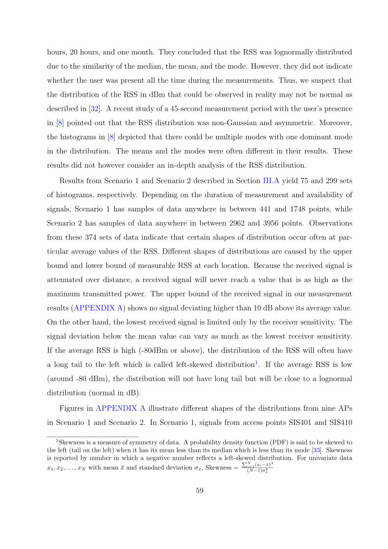
hours, 20 hours, and one month. They concluded that the RSS was lognormally distributed
due to the similarity of the median, the mean, and the mode. However, they did not indicate
whether the user was present all the time during the measurements. Thus, we suspect that
the distribution of the RSS in dBm that could be observed in reality may not be normal as
described in [32]. A recent study of a 45-second measurement period with the user’s presence
in [8] pointed out that the RSS distribution was non-Gaussian and asymmetric. Moreover,
the histograms in [8] depicted that there could be multiple modes with one dominant mode
in the distribution. The means and the modes were often different in their results. These
results did not however consider an in-depth analysis of the RSS distribution.
Results from Scenario 1 and Scenario 2 described in Section III.A yield 75 and 299 sets
of histograms, respectively. Depending on the duration of measurement and availability of
signals, Scenario 1 has samples of data anywhere in between 441 and 1748 points, while
Scenario 2 has samples of data anywhere in between 2962 and 3956 points. Observations
from these 374 sets of data indicate that certain shapes of distribution occur often at par-
ticular average values of the RSS. Different shapes of distributions are caused by the upper
bound and lower bound of measurable RSS at each location. Because the received signal is
attenuated over distance, a received signal will never reach a value that is as high as the
maximum transmitted power. The upper bound of the received signal in our measurement
results (APPENDIX A) shows no signal deviating higher than 10 dB above its average value.
On the other hand, the lowest received signal is limited only by the receiver sensitivity. The
signal deviation below the mean value can vary as much as the lowest receiver sensitivity.
If the average RSS is high (-80dBm or above), the distribution of the RSS will often have
a long tail to the left which is called left-skewed distribution1. If the average RSS is low
(around -80 dBm), the distribution will not have long tail but will be close to a lognormal
distribution (normal in dB).
Figures in APPENDIX A illustrate different shapes of the distributions from nine APs
in Scenario 1 and Scenario 2. In Scenario 1, signals from access points SIS401 and SIS410
1Skewness is a measure of symmetry of data. A probability density function (PDF) is said to be skewed tothe left (tail on the left) when it has its mean less than its median which is less than its mode [33]. Skewnessis reported by number in which a negative number reflects a left-skewed distribution. For univariate datax1, x2, . . . , xN with mean x̄ and standard deviation σx, Skewness =
PNi=1(xi−x̄)3
(N−1)σ3x
59
are stronger on average than those from SIS501 which is located a floor higher. Signals
from both SIS401 in Figure 60 and SIS410 in Figure 59 have larger deviations, primarily
to the left side, while distributions of signals from SIS501 are almost symmetric as seen
in Figure 61. In Scenario 2, similar shapes with long left tails are seen in Figure 62 and
Figure 66. Almost symmetric shapes of the histogram are observed in Figure 64, Figure 63,
Figure 65, and Figure 67. Note that histograms with multiple modes rarely occurred in both
scenarios which is in contrast to the results in [8]. Signals measured with different makes of
cards at the same location on majority also exhibit left-skewness as shown in Figure 13.
Proxim Cisco D−Link L−Gold L−Silver SMC−3
−2.5
−2
−1.5
−1
−0.5
0
0.5
1
Vendor
Ske
wne
ss
11/29/0411/30/0412/01/0412/01/0412/02/0412/05/04
Figure 13: Comparing Skewness of different vendors
To determine whether the data is significantly left-skewed, we compare skewness of each
data set with its standard error of skewness. The standard error of skewness can be estimated
by√
6N
where N is the number of data points [55]. If an absolute value of skewness is larger
than two standard errors of skewness, the data set is considered to be significantly skewed.
The distributions tended to be left-skewed in most measurement results from both scenarios.
In Scenario 1, we observed that 64 out of 75 histograms were significantly left-skewed, while
7 histograms were symmetric and 4 histograms were significantly right-skewed. In Scenario
2, we found that 191 out of 299 histograms were significantly left-skewed, while 51 of the
60
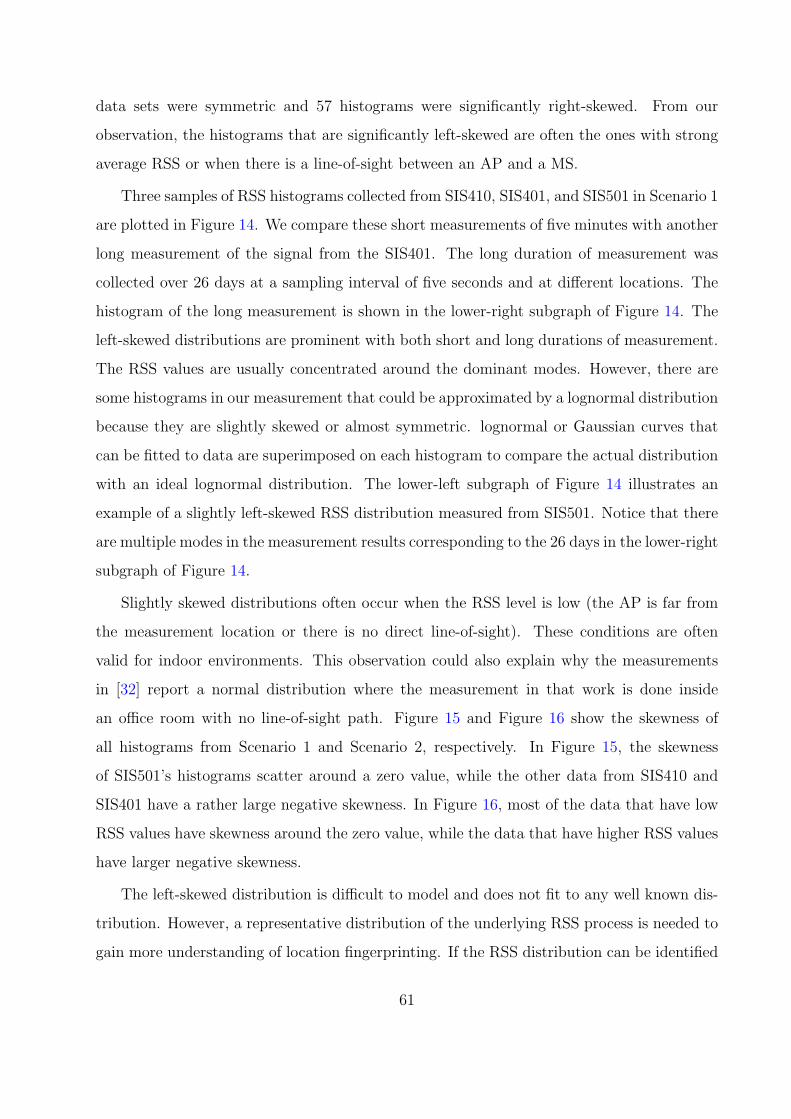
data sets were symmetric and 57 histograms were significantly right-skewed. From our
observation, the histograms that are significantly left-skewed are often the ones with strong
average RSS or when there is a line-of-sight between an AP and a MS.
Three samples of RSS histograms collected from SIS410, SIS401, and SIS501 in Scenario 1
are plotted in Figure 14. We compare these short measurements of five minutes with another
long measurement of the signal from the SIS401. The long duration of measurement was
collected over 26 days at a sampling interval of five seconds and at different locations. The
histogram of the long measurement is shown in the lower-right subgraph of Figure 14. The
left-skewed distributions are prominent with both short and long durations of measurement.
The RSS values are usually concentrated around the dominant modes. However, there are
some histograms in our measurement that could be approximated by a lognormal distribution
because they are slightly skewed or almost symmetric. lognormal or Gaussian curves that
can be fitted to data are superimposed on each histogram to compare the actual distribution
with an ideal lognormal distribution. The lower-left subgraph of Figure 14 illustrates an
example of a slightly left-skewed RSS distribution measured from SIS501. Notice that there
are multiple modes in the measurement results corresponding to the 26 days in the lower-right
subgraph of Figure 14.
Slightly skewed distributions often occur when the RSS level is low (the AP is far from
the measurement location or there is no direct line-of-sight). These conditions are often
valid for indoor environments. This observation could also explain why the measurements
in [32] report a normal distribution where the measurement in that work is done inside
an office room with no line-of-sight path. Figure 15 and Figure 16 show the skewness of
all histograms from Scenario 1 and Scenario 2, respectively. In Figure 15, the skewness
of SIS501’s histograms scatter around a zero value, while the other data from SIS410 and
SIS401 have a rather large negative skewness. In Figure 16, most of the data that have low
RSS values have skewness around the zero value, while the data that have higher RSS values
have larger negative skewness.
The left-skewed distribution is difficult to model and does not fit to any well known dis-
tribution. However, a representative distribution of the underlying RSS process is needed to
gain more understanding of location fingerprinting. If the RSS distribution can be identified
61
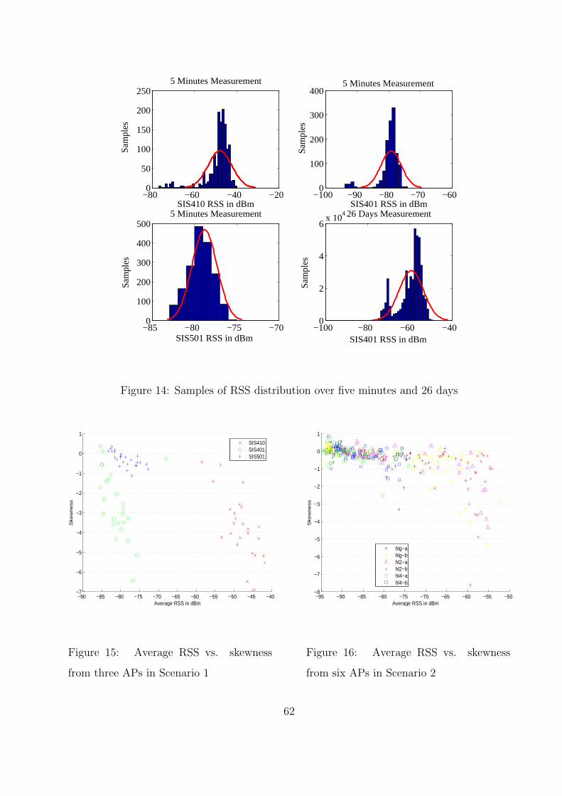
−80 −60 −40 −200
50
100
150
200
250
SIS410 RSS in dBm
Sam
ples
5 Minutes Measurement
−100 −90 −80 −70 −600
100
200
300
400
SIS401 RSS in dBm
Sam
ples
5 Minutes Measurement
−85 −80 −75 −700
100
200
300
400
500
SIS501 RSS in dBm
Sam
ples
5 Minutes Measurement
−100 −80 −60 −400
2
4
6x 10
4
SIS401 RSS in dBm
Sam
ples
26 Days Measurement
Figure 14: Samples of RSS distribution over five minutes and 26 days
−90 −85 −80 −75 −70 −65 −60 −55 −50 −45 −40−7
−6
−5
−4
−3
−2
−1
0
1
Average RSS in dBm
Ske
wn
ess
SIS410SIS401SIS501
Figure 15: Average RSS vs. skewness
from three APs in Scenario 1
−95 −90 −85 −80 −75 −70 −65 −60 −55 −50−8
−7
−6
−5
−4
−3
−2
−1
0
1
Average RSS in dBm
Ske
wn
ess
hlg−ahlg−bhl2−ahl2−bhl4−ahl4−b
Figure 16: Average RSS vs. skewness
from six APs in Scenario 2
62
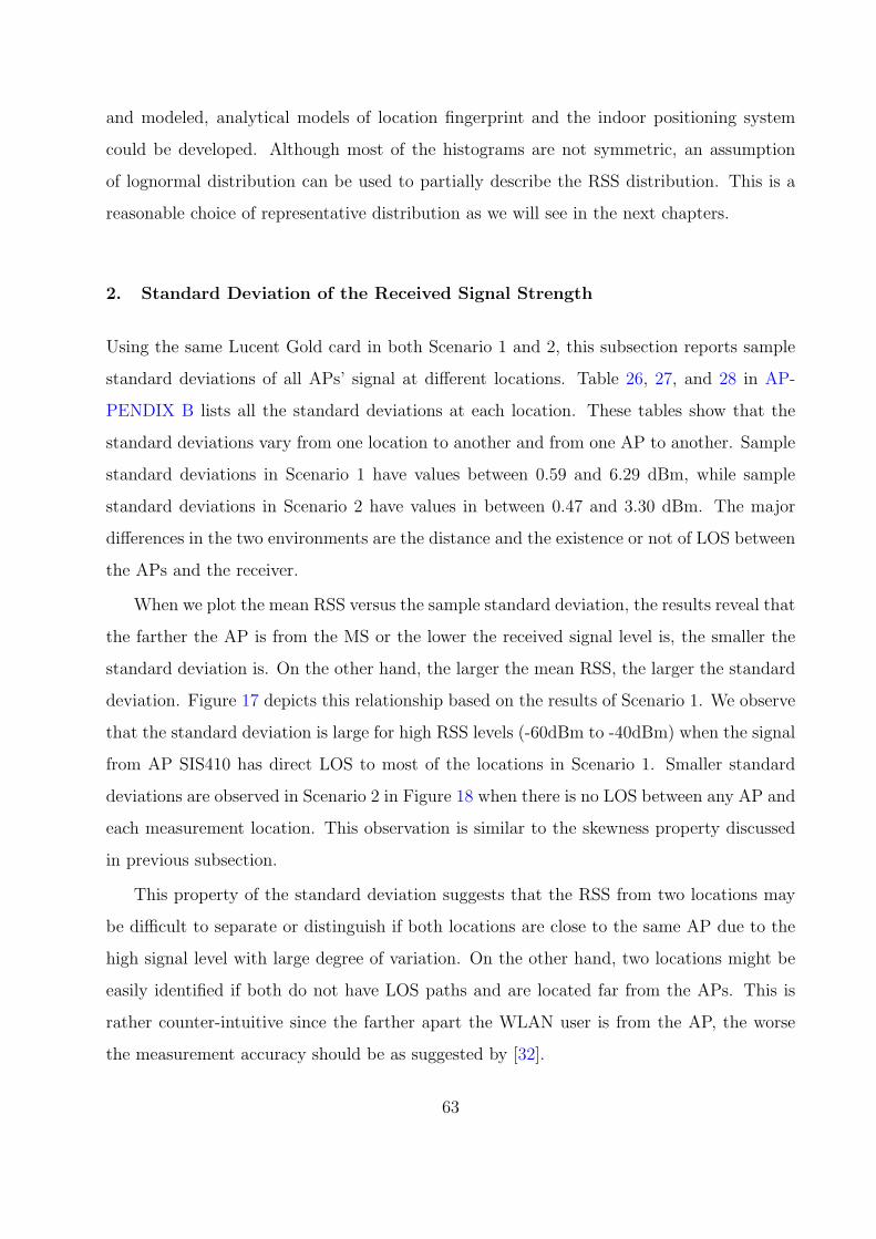
and modeled, analytical models of location fingerprint and the indoor positioning system
could be developed. Although most of the histograms are not symmetric, an assumption
of lognormal distribution can be used to partially describe the RSS distribution. This is a
reasonable choice of representative distribution as we will see in the next chapters.
2. Standard Deviation of the Received Signal Strength
Using the same Lucent Gold card in both Scenario 1 and 2, this subsection reports sample
standard deviations of all APs’ signal at different locations. Table 26, 27, and 28 in AP-
PENDIX B lists all the standard deviations at each location. These tables show that the
standard deviations vary from one location to another and from one AP to another. Sample
standard deviations in Scenario 1 have values between 0.59 and 6.29 dBm, while sample
standard deviations in Scenario 2 have values in between 0.47 and 3.30 dBm. The major
differences in the two environments are the distance and the existence or not of LOS between
the APs and the receiver.
When we plot the mean RSS versus the sample standard deviation, the results reveal that
the farther the AP is from the MS or the lower the received signal level is, the smaller the
standard deviation is. On the other hand, the larger the mean RSS, the larger the standard
deviation. Figure 17 depicts this relationship based on the results of Scenario 1. We observe
that the standard deviation is large for high RSS levels (-60dBm to -40dBm) when the signal
from AP SIS410 has direct LOS to most of the locations in Scenario 1. Smaller standard
deviations are observed in Scenario 2 in Figure 18 when there is no LOS between any AP and
each measurement location. This observation is similar to the skewness property discussed
in previous subsection.
This property of the standard deviation suggests that the RSS from two locations may
be difficult to separate or distinguish if both locations are close to the same AP due to the
high signal level with large degree of variation. On the other hand, two locations might be
easily identified if both do not have LOS paths and are located far from the APs. This is
rather counter-intuitive since the farther apart the WLAN user is from the AP, the worse
the measurement accuracy should be as suggested by [32].
63
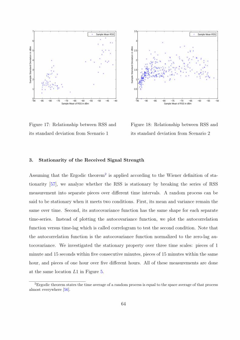
−90 −85 −80 −75 −70 −65 −60 −55 −50 −45 −400
1
2
3
4
5
6
7
Sample Mean of RSS in dBm
Sa
mp
le S
tan
da
rd D
evi
atio
n in
dB
m
Sample Mean RSS
Figure 17: Relationship between RSS and
its standard deviation from Scenario 1
−95 −90 −85 −80 −75 −70 −65 −60 −55 −500
0.5
1
1.5
2
2.5
3
3.5
Sample Mean of RSS in dBm
Sa
mp
le S
tan
da
rd D
evi
atio
n in
dB
m
Sample Mean RSS
Figure 18: Relationship between RSS and
its standard deviation from Scenario 2
3. Stationarity of the Received Signal Strength
Assuming that the Ergodic theorem2 is applied according to the Wiener definition of sta-
tionarity [57], we analyze whether the RSS is stationary by breaking the series of RSS
measurement into separate pieces over different time intervals. A random process can be
said to be stationary when it meets two conditions. First, its mean and variance remain the
same over time. Second, its autocovariance function has the same shape for each separate
time-series. Instead of plotting the autocovariance function, we plot the autocorrelation
function versus time-lag which is called correlogram to test the second condition. Note that
the autocorrelation function is the autocovariance function normalized to the zero-lag au-
tocovariance. We investigated the stationary property over three time scales: pieces of 1
minute and 15 seconds within five consecutive minutes, pieces of 15 minutes within the same
hour, and pieces of one hour over five different hours. All of these measurements are done
at the same location L1 in Figure 5.
2Ergodic theorem states the time average of a random process is equal to the space average of that processalmost everywhere [56].
64
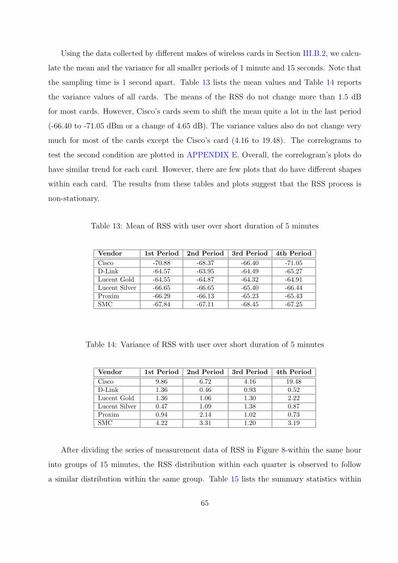
Using the data collected by different makes of wireless cards in Section III.B.2, we calcu-
late the mean and the variance for all smaller periods of 1 minute and 15 seconds. Note that
the sampling time is 1 second apart. Table 13 lists the mean values and Table 14 reports
the variance values of all cards. The means of the RSS do not change more than 1.5 dB
for most cards. However, Cisco’s cards seem to shift the mean quite a lot in the last period
(-66.40 to -71.05 dBm or a change of 4.65 dB). The variance values also do not change very
much for most of the cards except the Cisco’s card (4.16 to 19.48). The correlograms to
test the second condition are plotted in APPENDIX E. Overall, the correlogram’s plots do
have similar trend for each card. However, there are few plots that do have different shapes
within each card. The results from these tables and plots suggest that the RSS process is
non-stationary.
Table 13: Mean of RSS with user over short duration of 5 minutes
Vendor 1st Period 2nd Period 3rd Period 4th PeriodCisco -70.88 -68.37 -66.40 -71.05D-Link -64.57 -63.95 -64.49 -65.27Lucent Gold -64.55 -64.87 -64.32 -64.91Lucent Silver -66.65 -66.65 -65.40 -66.44Proxim -66.29 -66.13 -65.23 -65.43SMC -67.84 -67.11 -68.45 -67.25
Table 14: Variance of RSS with user over short duration of 5 minutes
Vendor 1st Period 2nd Period 3rd Period 4th PeriodCisco 9.86 6.72 4.16 19.48D-Link 1.36 0.46 0.93 0.52Lucent Gold 1.36 1.06 1.30 2.22Lucent Silver 0.47 1.09 1.38 0.87Proxim 0.94 2.14 1.02 0.73SMC 4.22 3.31 1.20 3.19
After dividing the series of measurement data of RSS in Figure 8-within the same hour
into groups of 15 minutes, the RSS distribution within each quarter is observed to follow
a similar distribution within the same group. Table 15 lists the summary statistics within
65
each quarter-hour. These results suggest that the RSS distribution may be stationary or
time independent since the means are very close (less than 2 dB difference) and the sample
variances of each quarter are on the same order. The correlograms in Figure 19 depict the
same shapes for each quarter indicating that the second condition is also met for this time
scale.
Table 15: Mean and standard deviation of RSS with user
Statistics 1st Qtr. 2nd Qtr. 3rd Qtr. 4th Qtr.Mean -71.71 -72.33 -71.82 -70.48
Standard Deviation 2.95 3.20 2.96 2.56Sample Variance 8.72 10.27 8.77 6.54
0 5 10 15 20−0.5
0
0.5
1
Time lag in second
Aut
ocor
rela
tion
Correlogram of 1st Quarter
0 5 10 15 20−0.5
0
0.5
1
Time lag in second
Aut
ocor
rela
tion
Correlogram of 2nd Quarter
0 5 10 15 20−0.5
0
0.5
1
Time lag in second
Aut
ocor
rela
tion
Correlogram of 3rd Quarter
0 5 10 15 20−0.5
0
0.5
1
Time lag in second
Aut
ocor
rela
tion
Correlogram of 4th Quarter
Figure 19: Correlograms of RSS within the same hour
The one-hour time scale study was made for a signal measured at L1 over different times
of day. Table 16 shows a consistent mean, but inconsistent variance values of the RSS.
Therefore, the test for the first condition for stationarity fails at this time scale and we
conclude that the RSS random process is non-stationary.
Another result indicating the non stationary property of the RSS is shown in Figure 20.
The measurement was recorded over a period of one hour from three access point at location
66
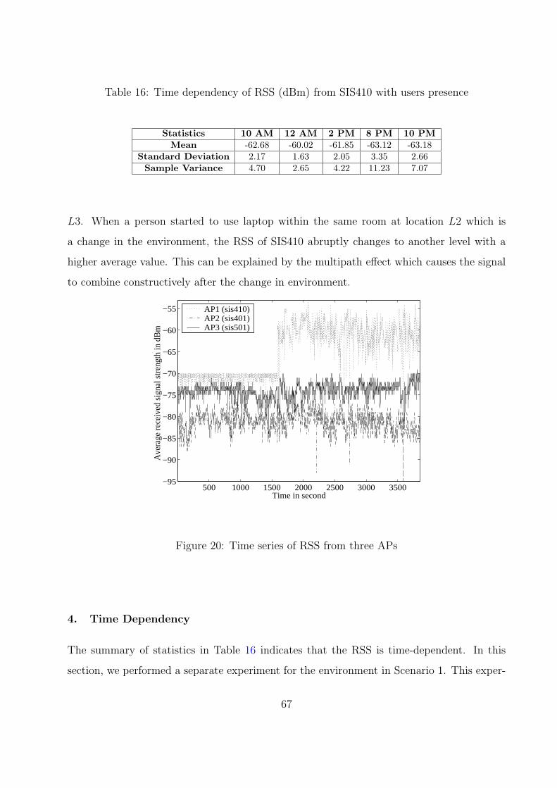
Table 16: Time dependency of RSS (dBm) from SIS410 with users presence
Statistics 10 AM 12 AM 2 PM 8 PM 10 PMMean -62.68 -60.02 -61.85 -63.12 -63.18
Standard Deviation 2.17 1.63 2.05 3.35 2.66Sample Variance 4.70 2.65 4.22 11.23 7.07
L3. When a person started to use laptop within the same room at location L2 which is
a change in the environment, the RSS of SIS410 abruptly changes to another level with a
higher average value. This can be explained by the multipath effect which causes the signal
to combine constructively after the change in environment.
500 1000 1500 2000 2500 3000 3500−95
−90
−85
−80
−75
−70
−65
−60
−55
Time in second
Ave
rage
rec
eive
d si
gnal
str
engt
h in
dB
m
AP1 (sis410)AP2 (sis401)AP3 (sis501)
Figure 20: Time series of RSS from three APs
4. Time Dependency
The summary of statistics in Table 16 indicates that the RSS is time-dependent. In this
section, we performed a separate experiment for the environment in Scenario 1. This exper-
67
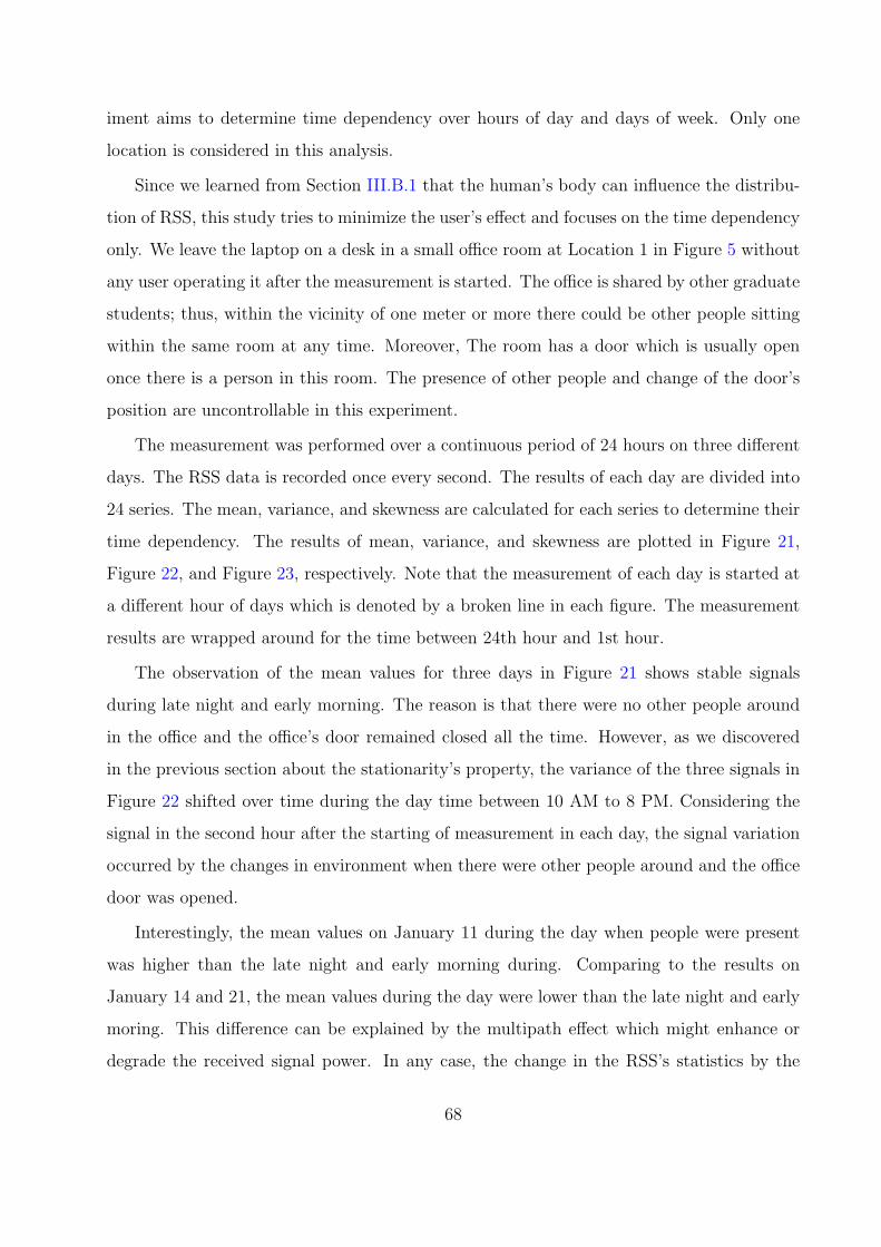
iment aims to determine time dependency over hours of day and days of week. Only one
location is considered in this analysis.
Since we learned from Section III.B.1 that the human’s body can influence the distribu-
tion of RSS, this study tries to minimize the user’s effect and focuses on the time dependency
only. We leave the laptop on a desk in a small office room at Location 1 in Figure 5 without
any user operating it after the measurement is started. The office is shared by other graduate
students; thus, within the vicinity of one meter or more there could be other people sitting
within the same room at any time. Moreover, The room has a door which is usually open
once there is a person in this room. The presence of other people and change of the door’s
position are uncontrollable in this experiment.
The measurement was performed over a continuous period of 24 hours on three different
days. The RSS data is recorded once every second. The results of each day are divided into
24 series. The mean, variance, and skewness are calculated for each series to determine their
time dependency. The results of mean, variance, and skewness are plotted in Figure 21,
Figure 22, and Figure 23, respectively. Note that the measurement of each day is started at
a different hour of days which is denoted by a broken line in each figure. The measurement
results are wrapped around for the time between 24th hour and 1st hour.
The observation of the mean values for three days in Figure 21 shows stable signals
during late night and early morning. The reason is that there were no other people around
in the office and the office’s door remained closed all the time. However, as we discovered
in the previous section about the stationarity’s property, the variance of the three signals in
Figure 22 shifted over time during the day time between 10 AM to 8 PM. Considering the
signal in the second hour after the starting of measurement in each day, the signal variation
occurred by the changes in environment when there were other people around and the office
door was opened.
Interestingly, the mean values on January 11 during the day when people were present
was higher than the late night and early morning during. Comparing to the results on
January 14 and 21, the mean values during the day were lower than the late night and early
moring. This difference can be explained by the multipath effect which might enhance or
degrade the received signal power. In any case, the change in the RSS’s statistics by the
68
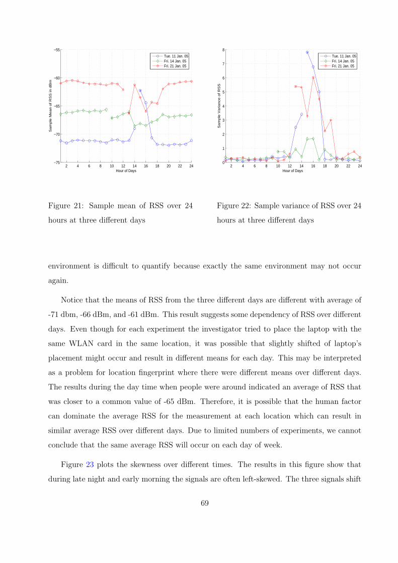
2 4 6 8 10 12 14 16 18 20 22 24−75
−70
−65
−60
−55
Hour of Days
Sa
mp
le M
ea
n o
f R
SS
in d
Bm
Tue. 11 Jan. 05Fri. 14 Jan. 05Fri. 21 Jan. 05
Figure 21: Sample mean of RSS over 24
hours at three different days
2 4 6 8 10 12 14 16 18 20 22 240
1
2
3
4
5
6
7
8
Hour of Days
Sa
mple
Variance
of R
SS
Tue. 11 Jan. 05Fri. 14 Jan. 05Fri. 21 Jan. 05
Figure 22: Sample variance of RSS over 24
hours at three different days
environment is difficult to quantify because exactly the same environment may not occur
again.
Notice that the means of RSS from the three different days are different with average of
-71 dbm, -66 dBm, and -61 dBm. This result suggests some dependency of RSS over different
days. Even though for each experiment the investigator tried to place the laptop with the
same WLAN card in the same location, it was possible that slightly shifted of laptop’s
placement might occur and result in different means for each day. This may be interpreted
as a problem for location fingerprint where there were different means over different days.
The results during the day time when people were around indicated an average of RSS that
was closer to a common value of -65 dBm. Therefore, it is possible that the human factor
can dominate the average RSS for the measurement at each location which can result in
similar average RSS over different days. Due to limited numbers of experiments, we cannot
conclude that the same average RSS will occur on each day of week.
Figure 23 plots the skewness over different times. The results in this figure show that
during late night and early morning the signals are often left-skewed. The three signals shift
69
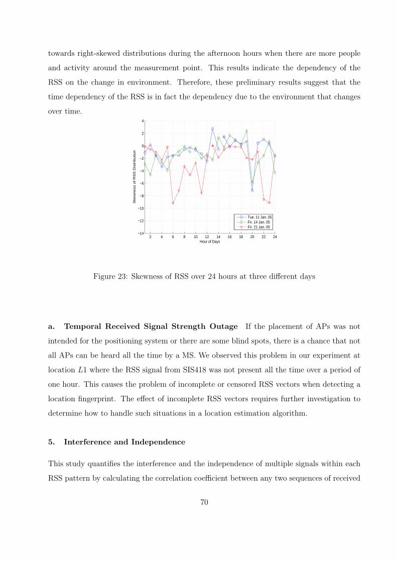
towards right-skewed distributions during the afternoon hours when there are more people
and activity around the measurement point. This results indicate the dependency of the
RSS on the change in environment. Therefore, these preliminary results suggest that the
time dependency of the RSS is in fact the dependency due to the environment that changes
over time.
2 4 6 8 10 12 14 16 18 20 22 24−14
−12
−10
−8
−6
−4
−2
0
2
4
Hour of Days
Ske
wn
ess
of R
SS
Dis
trib
utio
n
Tue. 11 Jan. 05Fri. 14 Jan. 05Fri. 21 Jan. 05
Figure 23: Skewness of RSS over 24 hours at three different days
a. Temporal Received Signal Strength Outage If the placement of APs was not
intended for the positioning system or there are some blind spots, there is a chance that not
all APs can be heard all the time by a MS. We observed this problem in our experiment at
location L1 where the RSS signal from SIS418 was not present all the time over a period of
one hour. This causes the problem of incomplete or censored RSS vectors when detecting a
location fingerprint. The effect of incomplete RSS vectors requires further investigation to
determine how to handle such situations in a location estimation algorithm.
5. Interference and Independence
This study quantifies the interference and the independence of multiple signals within each
RSS pattern by calculating the correlation coefficient between any two sequences of received
70
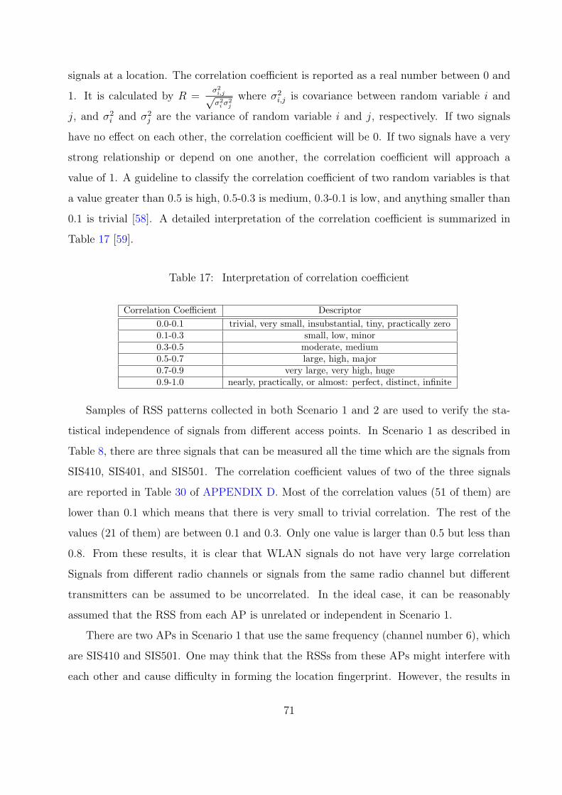
signals at a location. The correlation coefficient is reported as a real number between 0 and
1. It is calculated by R =σ2
i,j√σ2
i σ2j
where σ2i,j is covariance between random variable i and
j, and σ2i and σ2
j are the variance of random variable i and j, respectively. If two signals
have no effect on each other, the correlation coefficient will be 0. If two signals have a very
strong relationship or depend on one another, the correlation coefficient will approach a
value of 1. A guideline to classify the correlation coefficient of two random variables is that
a value greater than 0.5 is high, 0.5-0.3 is medium, 0.3-0.1 is low, and anything smaller than
0.1 is trivial [58]. A detailed interpretation of the correlation coefficient is summarized in
Table 17 [59].
Table 17: Interpretation of correlation coefficient
Correlation Coefficient Descriptor0.0-0.1 trivial, very small, insubstantial, tiny, practically zero0.1-0.3 small, low, minor0.3-0.5 moderate, medium0.5-0.7 large, high, major0.7-0.9 very large, very high, huge0.9-1.0 nearly, practically, or almost: perfect, distinct, infinite
Samples of RSS patterns collected in both Scenario 1 and 2 are used to verify the sta-
tistical independence of signals from different access points. In Scenario 1 as described in
Table 8, there are three signals that can be measured all the time which are the signals from
SIS410, SIS401, and SIS501. The correlation coefficient values of two of the three signals
are reported in Table 30 of APPENDIX D. Most of the correlation values (51 of them) are
lower than 0.1 which means that there is very small to trivial correlation. The rest of the
values (21 of them) are between 0.1 and 0.3. Only one value is larger than 0.5 but less than
0.8. From these results, it is clear that WLAN signals do not have very large correlation
Signals from different radio channels or signals from the same radio channel but different
transmitters can be assumed to be uncorrelated. In the ideal case, it can be reasonably
assumed that the RSS from each AP is unrelated or independent in Scenario 1.
There are two APs in Scenario 1 that use the same frequency (channel number 6), which
are SIS410 and SIS501. One may think that the RSSs from these APs might interfere with
each other and cause difficulty in forming the location fingerprint. However, the results in
71
the third column of Table 30 of APPENDIX D indicate that both RSSs have only low to tiny
correlation. The signals do not interfere with each other. Therefore, access points using the
same radio frequency do not have any significant impact on the location fingerprint. This
could be explained by the collision avoidance mechanism of the IEEE 802.11b [48] which
enables a clear signal reception.
In Scenario 2, there are six signals available inside a large hall environment as described
in Table 8. Because the area in this scenario is larger than the first one, not all signals
can be measured at every location. Table 31, Table 32, and Table 33 of APPENDIX D
summarize the correlation coefficients for the access points with radio channels 1 and 6, 1
and 11, and 6 and 11, respectively. Table 34, Table 35, and Table 36 of APPENDIX D report
the correlation coefficients for those access points using the same radio channel. Only four
correlation coefficients from these six tables are in between 0.5 and 0.3, while 90 of them are
in between 0.3 and 0.1 and 175 of them are less than 0.1. These results suggest that there
is moderate to very small correlation between any received signal pair. Once again, these
results can lead to the reasonable assumption that the RSS from each AP is unrelated or
independent in Scenario 2.
6. Required Number of Samples
Collecting enough statistics for creating location fingerprints is the key to achieving good
performance with any indoor positioning system (either distance based or probabilistic ap-
proach). If the positioning system requires only the mean values to create fingerprints, a
small number of samples is sufficient since the mean is relatively constant. Ideally, we would
like to have as many samples as possible. In the literature, a small number on the order
of 20 samples per location and orientation is used with acceptable location determination
performance in RADAR [13]. Larger numbers of samples are required for the probabilistic
approach to create accurate histograms. Youssef et al [60] and Xiang et al [17] recorded 300
samples per location and orientation.
The duration of data collection in the literature are different due to the sampling period.
For instance, RADAR [13] used a 0.25-second sampling period, while Xiang et al [17] used
72
a two-second sampling period. The sampling period is limited by either the software or the
hardware. The software’s limits depend on how often can a device driver be accessed and
how often the BSSID scan list is updated. Some wireless cards have the capability to scan for
APs’ signal in the background [52]. Our prototype software-based indoor positioning system
in Chapter V limits our access to the scanning function to one second. The hardware’s limits
depend on how the vendor implements the scanning cycle and the amount of the channel
dwelling time. Clearly, it is difficult to obtain these limits because the information may be
proprietary for each vendor. However, Microsoft specifies that a scanning query must be
returned within two seconds after the query command is initiated [52].
To study the required number of samples, we randomly select sets of RSS measurement
data from all access points in both scenarios. Then, we calculate summary statistics of
each AP with different numbers of samples ranging from 30, 50, 100, 150, 200, 300, and the
maximum amount of collected data. Assuming that the maximum amount of collected data
represents the most accurate distribution of RSS at that location, we compare the summary
statistics of each number of samples. APPENDIX F lists the tables of these statistics. By
inspection, it is true that only small numbers of samples (30 and 50) would be sufficient for
a location fingerprint based on the mean values only. If we approximate the distribution of
RSS using the lognormal distribution, the distribution can be completely described by the
mean and the variance. Therefore, the convergence of standard deviation can be used as
a condition to stop collecting new samples. From the tables in APPENDIX F, a number
between 150 and 200 should be sufficient.
D. CAUSES OF ERROR IN LOCATION DETECTION
The randomness of RSS is the major cause of error in in any indoor positioning system that
uses the RSS for location inference. If there was no randomness in the RSS and its location
fingerprint, every indoor positioning systems of this type will have no location detection error
(excellent accuracy and precision performance). In this section, we investigate the causes
of error in identifying any indoor locations. First, we discuss the error based on the results
73
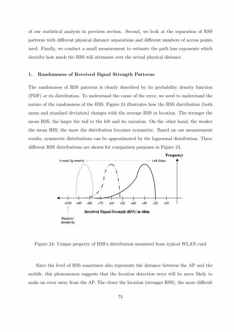
of our statistical analysis in previous section. Second, we look at the separation of RSS
patterns with different physical distance separations and different numbers of access points
used. Finally, we conduct a small measurement to estimate the path loss exponents which
describe how much the RSS will attenuate over the actual physical distance.
1. Randomness of Received Signal Strength Patterns
The randomness of RSS patterns is clearly described by its probability density function
(PDF) or its distribution. To understand the cause of the error, we need to understand the
nature of the randomness of the RSS. Figure 24 illustrates how the RSS distribution (both
mean and standard deviation) changes with the average RSS or location. The stronger the
mean RSS, the larger the tail to the left and its variation. On the other hand, the weaker
the mean RSS, the more the distribution becomes symmetric. Based on our measurement
results, symmetric distributions can be approximated by the lognormal distribution. Three
different RSS distributions are shown for comparison purposes in Figure 24.
Received Signal Strength (RSS) in dBm -10-20-30-40-50-60-70-80-90-100FrequencyLeft-SkewAlmost Symmetric
ReceiverSensitivityFigure 24: Unique property of RSS’s distribution measured from typical WLAN card
Since the level of RSS sometimes also represents the distance between the AP and the
mobile, this phenomenon suggests that the location detection error will be more likely to
make an error away from the AP. The closer the location (stronger RSS), the more difficult
74
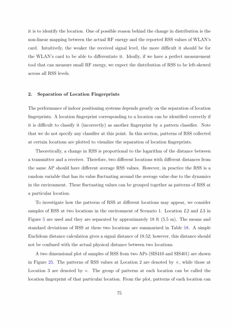
it is to identify the location. One of possible reason behind the change in distribution is the
non-linear mapping between the actual RF energy and the reported RSS values of WLAN’s
card. Intuitively, the weaker the received signal level, the more difficult it should be for
the WLAN’s card to be able to differentiate it. Ideally, if we have a perfect measurement
tool that can measure small RF energy, we expect the distribution of RSS to be left-skewed
across all RSS levels.
2. Separation of Location Fingerprints
The performance of indoor positioning systems depends greatly on the separation of location
fingerprints. A location fingerprint corresponding to a location can be identified correctly if
it is difficult to classify it (incorrectly) as another fingerprint by a pattern classifier. Note
that we do not specify any classifier at this point. In this section, patterns of RSS collected
at certain locations are plotted to visualize the separation of location fingerprints.
Theoretically, a change in RSS is proportional to the logarithm of the distance between
a transmitter and a receiver. Therefore, two different locations with different distances from
the same AP should have different average RSS values. However, in practice the RSS is a
random variable that has its value fluctuating around the average value due to the dynamics
in the environment. These fluctuating values can be grouped together as patterns of RSS at
a particular location.
To investigate how the patterns of RSS at different locations may appear, we consider
samples of RSS at two locations in the environment of Scenario 1. Location L2 and L3 in
Figure 5 are used and they are separated by approximately 18 ft (5.5 m). The means and
standard deviations of RSS at these two locations are summarized in Table 18. A simple
Euclidean distance calculation gives a signal distance of 18.52; however, this distance should
not be confused with the actual physical distance between two locations.
A two dimensional plot of samples of RSS from two APs (SIS410 and SIS401) are shown
in Figure 25. The patterns of RSS values at Location 2 are denoted by ×, while those at
Location 3 are denoted by ◦. The group of patterns at each location can be called the
location fingerprint of that particular location. From the plot, patterns of each location can
75
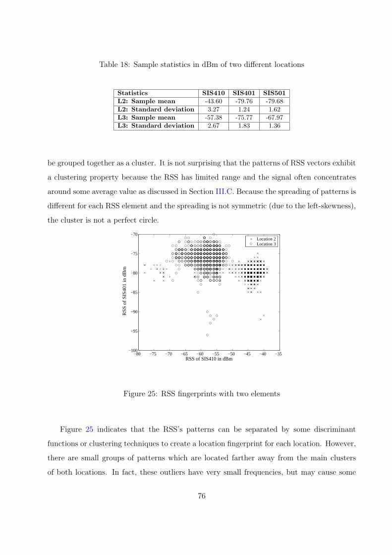
Table 18: Sample statistics in dBm of two different locations
Statistics SIS410 SIS401 SIS501L2: Sample mean -43.60 -79.76 -79.68L2: Standard deviation 3.27 1.24 1.62L3: Sample mean -57.38 -75.77 -67.97L3: Standard deviation 2.67 1.83 1.36
be grouped together as a cluster. It is not surprising that the patterns of RSS vectors exhibit
a clustering property because the RSS has limited range and the signal often concentrates
around some average value as discussed in Section III.C. Because the spreading of patterns is
different for each RSS element and the spreading is not symmetric (due to the left-skewness),
the cluster is not a perfect circle.
−80 −75 −70 −65 −60 −55 −50 −45 −40 −35−100
−95
−90
−85
−80
−75
−70
RSS of SIS410 in dBm
RS
S o
f S
IS4
01
in d
Bm
Location 2Location 3
Figure 25: RSS fingerprints with two elements
Figure 25 indicates that the RSS’s patterns can be separated by some discriminant
functions or clustering techniques to create a location fingerprint for each location. However,
there are small groups of patterns which are located farther away from the main clusters
of both locations. In fact, these outliers have very small frequencies, but may cause some
76
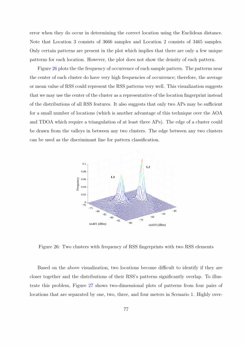
error when they do occur in determining the correct location using the Euclidean distance.
Note that Location 3 consists of 3666 samples and Location 2 consists of 3465 samples.
Only certain patterns are present in the plot which implies that there are only a few unique
patterns for each location. However, the plot does not show the density of each pattern.
Figure 26 plots the the frequency of occurrence of each sample pattern. The patterns near
the center of each cluster do have very high frequencies of occurrence; therefore, the average
or mean value of RSS could represent the RSS patterns very well. This visualization suggests
that we may use the center of the cluster as a representative of the location fingerprint instead
of the distributions of all RSS features. It also suggests that only two APs may be sufficient
for a small number of locations (which is another advantage of this technique over the AOA
and TDOA which require a triangulation of at least three APs). The edge of a cluster could
be drawn from the valleys in between any two clusters. The edge between any two clusters
can be used as the discriminant line for pattern classification.
−80−70
−60−50
−40
−95−90
−85−80
−75−70
0
0.02
0.04
0.06
0.08
0.1
sis410 (dBm)sis401 (dBm)
Fre
quen
cy L3
L2
Figure 26: Two clusters with frequency of RSS fingerprints with two RSS elements
Based on the above visualization, two locations become difficult to identify if they are
closer together and the distributions of their RSS’s patterns significantly overlap. To illus-
trate this problem, Figure 27 shows two-dimensional plots of patterns from four pairs of
locations that are separated by one, two, three, and four meters in Scenario 1. Highly over-
77
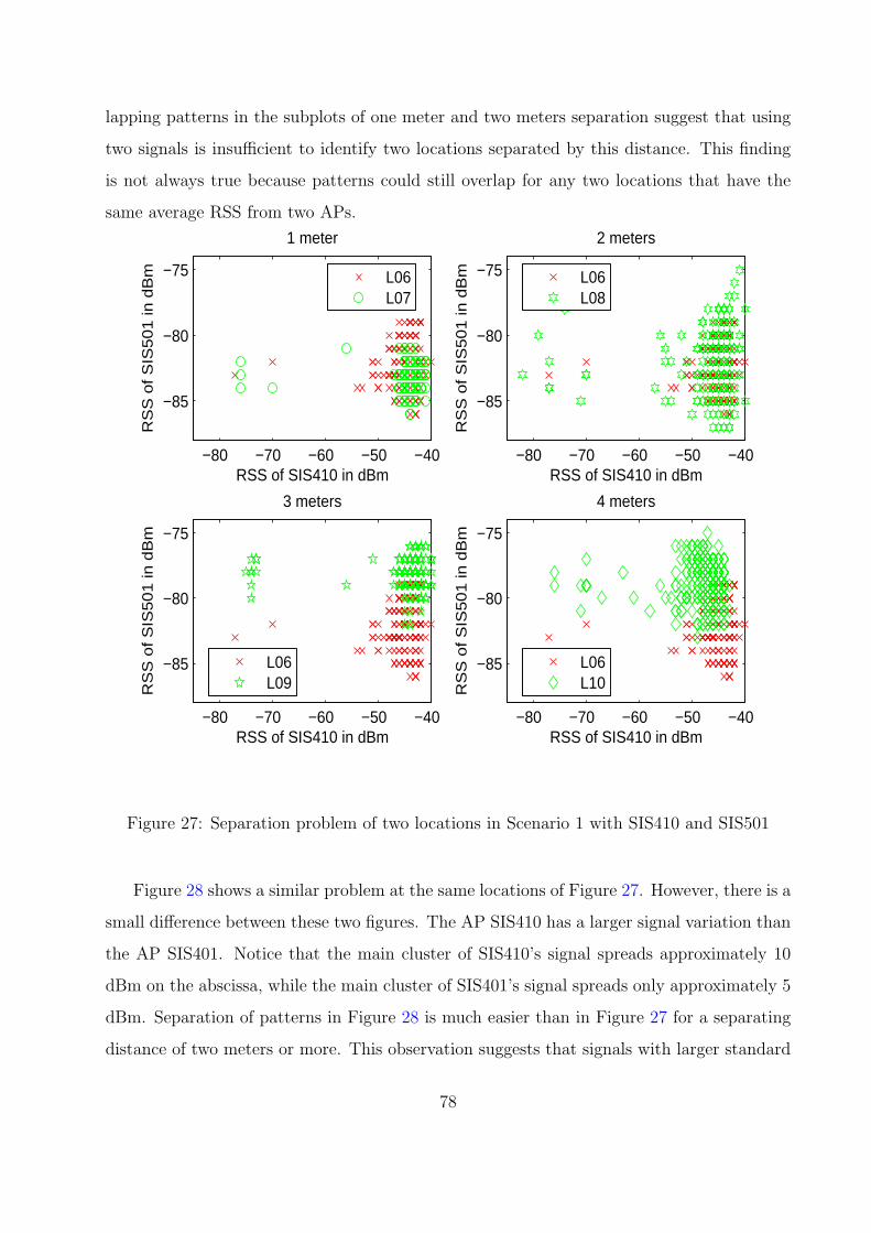
lapping patterns in the subplots of one meter and two meters separation suggest that using
two signals is insufficient to identify two locations separated by this distance. This finding
is not always true because patterns could still overlap for any two locations that have the
same average RSS from two APs.
−80 −70 −60 −50 −40
−85
−80
−75
RSS of SIS410 in dBm
RS
S o
f S
IS5
01
in d
Bm
1 meter
L06L07
−80 −70 −60 −50 −40
−85
−80
−75
RSS of SIS410 in dBmR
SS
of S
IS5
01
in d
Bm
2 meters
L06L08
−80 −70 −60 −50 −40
−85
−80
−75
RSS of SIS410 in dBm
RS
S o
f S
IS5
01
in d
Bm
3 meters
L06L09
−80 −70 −60 −50 −40
−85
−80
−75
RSS of SIS410 in dBm
RS
S o
f S
IS5
01
in d
Bm
4 meters
L06L10
Figure 27: Separation problem of two locations in Scenario 1 with SIS410 and SIS501
Figure 28 shows a similar problem at the same locations of Figure 27. However, there is a
small difference between these two figures. The AP SIS410 has a larger signal variation than
the AP SIS401. Notice that the main cluster of SIS410’s signal spreads approximately 10
dBm on the abscissa, while the main cluster of SIS401’s signal spreads only approximately 5
dBm. Separation of patterns in Figure 28 is much easier than in Figure 27 for a separating
distance of two meters or more. This observation suggests that signals with larger standard
78
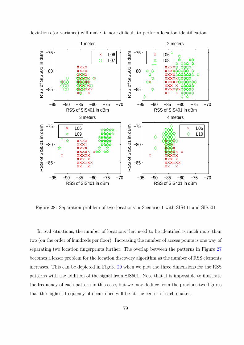
deviations (or variance) will make it more difficult to perform location identification.
−95 −90 −85 −80 −75 −70
−85
−80
−75
RSS of SIS401 in dBm
RS
S o
f S
IS5
01
in d
Bm
1 meter
L06L07
−95 −90 −85 −80 −75 −70
−85
−80
−75
RSS of SIS401 in dBm
RS
S o
f S
IS5
01
in d
Bm
2 meters
L06L08
−95 −90 −85 −80 −75 −70
−85
−80
−75
RSS of SIS401 in dBm
RS
S o
f S
IS5
01
in d
Bm
3 meters
L06L09
−95 −90 −85 −80 −75 −70
−85
−80
−75
RSS of SIS401 in dBm
RS
S o
f S
IS5
01
in d
Bm
4 meters
L06L10
Figure 28: Separation problem of two locations in Scenario 1 with SIS401 and SIS501
In real situations, the number of locations that need to be identified is much more than
two (on the order of hundreds per floor). Increasing the number of access points is one way of
separating two location fingerprints further. The overlap between the patterns in Figure 27
becomes a lesser problem for the location discovery algorithm as the number of RSS elements
increases. This can be depicted in Figure 29 when we plot the three dimensions for the RSS
patterns with the addition of the signal from SIS501. Note that it is impossible to illustrate
the frequency of each pattern in this case, but we may deduce from the previous two figures
that the highest frequency of occurrence will be at the center of each cluster.
79
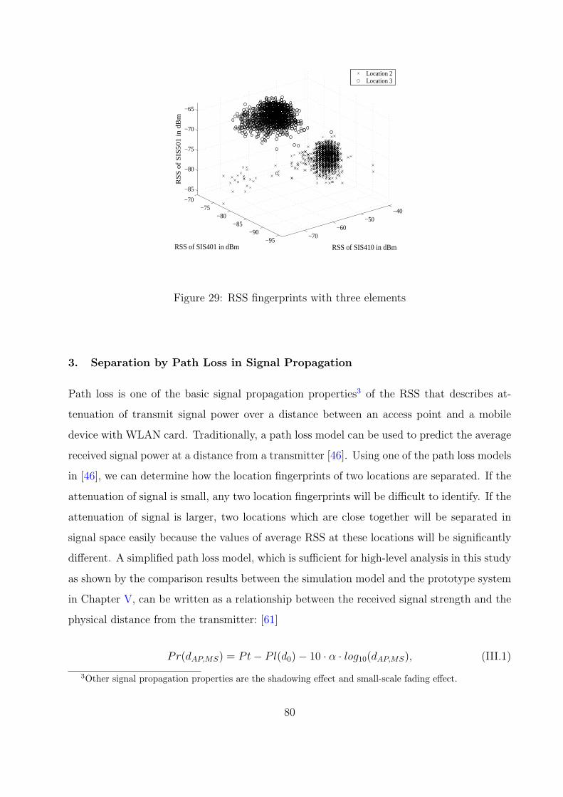
−70−60
−50−40
−95−90
−85−80
−75−70
−85
−80
−75
−70
−65
RSS of SIS410 in dBmRSS of SIS401 in dBm
RS
S o
f S
IS5
01
in d
Bm
Location 2Location 3
Figure 29: RSS fingerprints with three elements
3. Separation by Path Loss in Signal Propagation
Path loss is one of the basic signal propagation properties3 of the RSS that describes at-
tenuation of transmit signal power over a distance between an access point and a mobile
device with WLAN card. Traditionally, a path loss model can be used to predict the average
received signal power at a distance from a transmitter [46]. Using one of the path loss models
in [46], we can determine how the location fingerprints of two locations are separated. If the
attenuation of signal is small, any two location fingerprints will be difficult to identify. If the
attenuation of signal is larger, two locations which are close together will be separated in
signal space easily because the values of average RSS at these locations will be significantly
different. A simplified path loss model, which is sufficient for high-level analysis in this study
as shown by the comparison results between the simulation model and the prototype system
in Chapter V, can be written as a relationship between the received signal strength and the
physical distance from the transmitter: [61]
Pr(dAP,MS) = Pt− Pl(d0)− 10 · α · log10(dAP,MS), (III.1)
3Other signal propagation properties are the shadowing effect and small-scale fading effect.
80
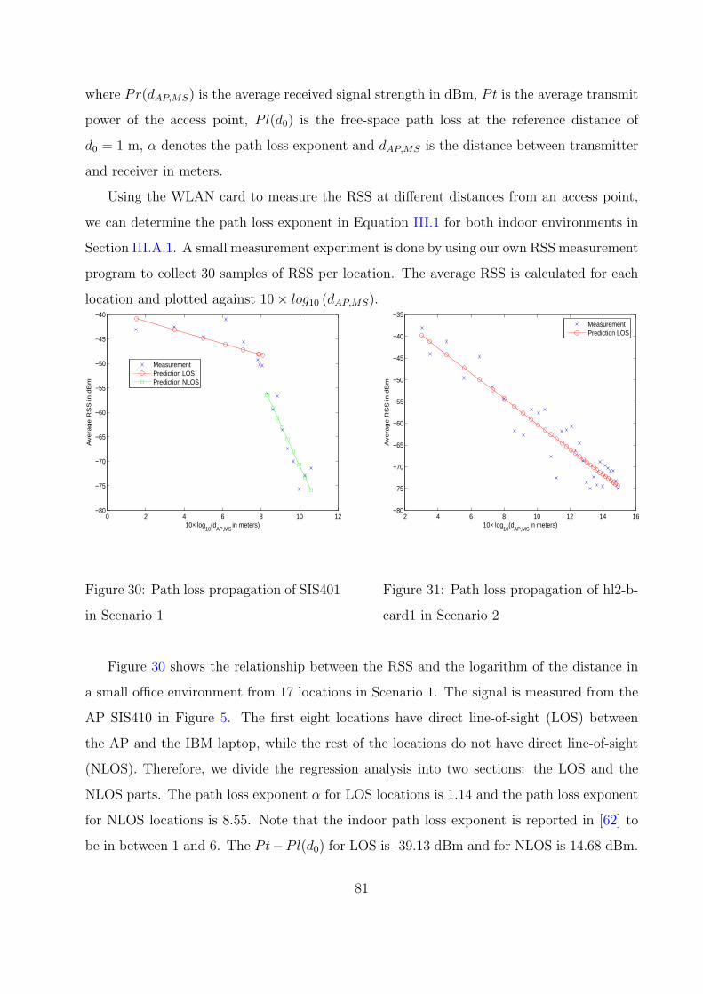
where Pr(dAP,MS) is the average received signal strength in dBm, Pt is the average transmit
power of the access point, Pl(d0) is the free-space path loss at the reference distance of
d0 = 1 m, α denotes the path loss exponent and dAP,MS is the distance between transmitter
and receiver in meters.
Using the WLAN card to measure the RSS at different distances from an access point,
we can determine the path loss exponent in Equation III.1 for both indoor environments in
Section III.A.1. A small measurement experiment is done by using our own RSS measurement
program to collect 30 samples of RSS per location. The average RSS is calculated for each
location and plotted against 10× log10 (dAP,MS).
0 2 4 6 8 10 12−80
−75
−70
−65
−60
−55
−50
−45
−40
10× log10
(dAP,MS
in meters)
Ave
rag
e R
SS
in d
Bm
MeasurementPrediction LOSPrediction NLOS
Figure 30: Path loss propagation of SIS401
in Scenario 1
2 4 6 8 10 12 14 16−80
−75
−70
−65
−60
−55
−50
−45
−40
−35
10× log10
(dAP,MS
in meters)
Ave
rag
e R
SS
in d
Bm
MeasurementPrediction LOS
Figure 31: Path loss propagation of hl2-b-
card1 in Scenario 2
Figure 30 shows the relationship between the RSS and the logarithm of the distance in
a small office environment from 17 locations in Scenario 1. The signal is measured from the
AP SIS410 in Figure 5. The first eight locations have direct line-of-sight (LOS) between
the AP and the IBM laptop, while the rest of the locations do not have direct line-of-sight
(NLOS). Therefore, we divide the regression analysis into two sections: the LOS and the
NLOS parts. The path loss exponent α for LOS locations is 1.14 and the path loss exponent
for NLOS locations is 8.55. Note that the indoor path loss exponent is reported in [62] to
be in between 1 and 6. The Pt−Pl(d0) for LOS is -39.13 dBm and for NLOS is 14.68 dBm.
81
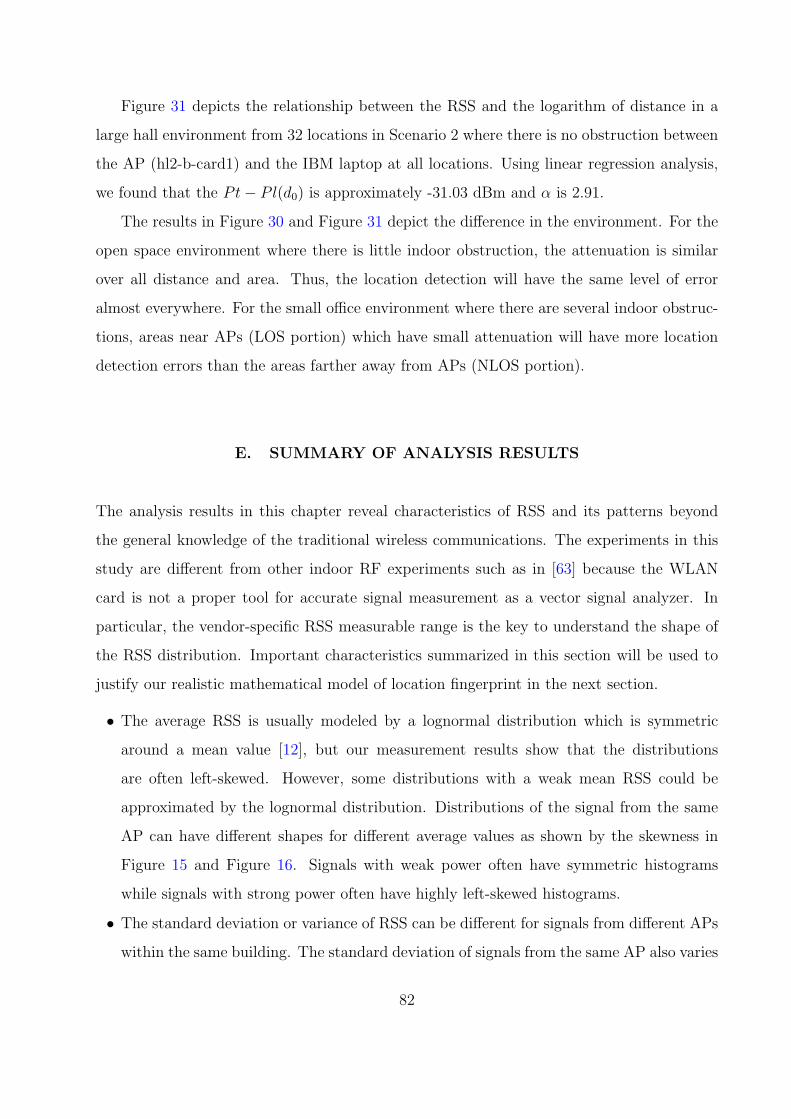
Figure 31 depicts the relationship between the RSS and the logarithm of distance in a
large hall environment from 32 locations in Scenario 2 where there is no obstruction between
the AP (hl2-b-card1) and the IBM laptop at all locations. Using linear regression analysis,
we found that the Pt− Pl(d0) is approximately -31.03 dBm and α is 2.91.
The results in Figure 30 and Figure 31 depict the difference in the environment. For the
open space environment where there is little indoor obstruction, the attenuation is similar
over all distance and area. Thus, the location detection will have the same level of error
almost everywhere. For the small office environment where there are several indoor obstruc-
tions, areas near APs (LOS portion) which have small attenuation will have more location
detection errors than the areas farther away from APs (NLOS portion).
E. SUMMARY OF ANALYSIS RESULTS
The analysis results in this chapter reveal characteristics of RSS and its patterns beyond
the general knowledge of the traditional wireless communications. The experiments in this
study are different from other indoor RF experiments such as in [63] because the WLAN
card is not a proper tool for accurate signal measurement as a vector signal analyzer. In
particular, the vendor-specific RSS measurable range is the key to understand the shape of
the RSS distribution. Important characteristics summarized in this section will be used to
justify our realistic mathematical model of location fingerprint in the next section.
• The average RSS is usually modeled by a lognormal distribution which is symmetric
around a mean value [12], but our measurement results show that the distributions
are often left-skewed. However, some distributions with a weak mean RSS could be
approximated by the lognormal distribution. Distributions of the signal from the same
AP can have different shapes for different average values as shown by the skewness in
Figure 15 and Figure 16. Signals with weak power often have symmetric histograms
while signals with strong power often have highly left-skewed histograms.
• The standard deviation or variance of RSS can be different for signals from different APs
within the same building. The standard deviation of signals from the same AP also varies
82
with the location as shown in APPENDIX B. The measurement results suggest that the
signal from APs at locations with direct line-of-sight (LOS) often has a large standard
deviation. On the other hand, the signal at non-line-of-sight (NLOS) locations often has
smaller standard deviations. In large building environments such as in Scenario 2, the
average of the standard deviation4 is smaller than in small building environments such
as in Scenario 1. We found that in Scenario 2 the average standard deviation of signals
from all APs are close together, while in Scenario 1 the average standard deviations are
quite different.
• When we consider the RSS at a location as a random process, we found that the random
process is typically non-stationary. Although the mean usually stays around the same
value, the variance could shift over long periods of time such as different hours of the day.
Moreover, the autocorrelation (autocovariance) function does not have the same shape
for each separate time-series. Changes in environment such as a human’s movement or
furniture relocation could also change the mean RSS. These non-stationary properties
indicate the difficulty in modeling RSS fingerprints for indoor positioning systems.
• Signals from different APs within the range of reception can be considered as independent
because the correlation coefficient between any pair of signals is often small or trivial.
The interference between the signals using the same radio frequency does not have any
strong correlation, thus the interference by the co-channel signals may have little effect
on the formation of the location fingerprint. The independence of signals is most likely
a result of the collision avoidance mechanism of the medium access control protocol in
802.11.
• The RSS patterns for a given location usually cluster around one or more values near
center of patterns that have high frequency of occurrence as shown in Figure 26. This
confirms that a vector of average values of RSS can be used to represent a location
fingerprint or a vector of means as done by RADAR system [13].
• There are two ways to improve the separation of RSS patterns: increase the distance
between two locations or add additional access points into the pattern consideration.
4Although average of standard deviation should not be calculated as a summary statistics, this studydoes so in order to find a representative value to model the whole scenario.
83
F. IMPLICATION ON MODELING OF LOCATION FINGERPRINT
To model the indoor positioning system based on location fingerprints, we need basic math-
ematical assumptions for location fingerprints. This section lists the set of assumptions that
are derived from the above analyses. These assumptions are proposed for their mathematical
tractability while still reflecting real RSS patterns to the extent possible.
• First of all, we assume that the random RSS is a stationary process. This is done to
eliminate time dependency properties of the RSS. We have seen that the mean is mostly
invariant over time. While the standard deviation will affect the performance, using
larger standard deviations will keep our performance results conservative.
• Each RSS element ρi in the location fingerprint F = (ρ1, ρ2, . . . , ρN)T is assumed to
be a lognormally distributed random variable which can be described by a mean and
a variance. Although measurement results show that the majority of RSS distributions
are non-symmetric and left-skewed, there are no well-known left-skewed distributions
available in the literature. Thus, it is difficult to construct mathematical analysis based
on a left-skewed distribution. When each RSS is assumed to be a lognormally distrib-
uted random variable, the location fingerprint becomes a multivariate lognormal random
variable or vector of N random variables from N APs. We will see in the next chapters
that this assumption gives a reasonable approximation of the performance.
• The (sample) mean ρn of each RSS (lognormally distribution) is assumed to be constant
for each location and corresponding fingerprint.
• The (sample) standard deviation σi of each RSS (lognormal distribution) is assumed to
be constant for each AP’s signal but can be different from one AP to another AP, σi 6= σj.
This assumption will cause our model to have less error in location detection because we
did not model the location-dependent standard deviation as described in Figure 24. For
further simplification, we also assume that the sample standard deviation is identical for
all locations and all APs in order to study the effect of one variable for the whole system.
• All AP’s signals are assumed to be independent. However, the correlation between each
pair of AP’s signal can be represented by a covariance σij in a covariance matrix C which
84
is constant and does not shift over time for all locations, C = E{(S −F)(S −F)T}. This
can be used to capture the small effects of correlation.
• The location fingerprint vector F is the vector of the true mean of the multivariate
Gaussian random variable S or sample RSS pattern which is measured during the on-
line phase, ρi = E{si} from access point i. We assume that the mean vectors do not
shift over time.
G. CONCLUSIONS
We presented an initial analysis of the RSS values reported by an 802.11b NIC commonly
used in indoor location systems based on location fingerprinting. We pointed out that the
user’s presence should be taken into account when collecting the location fingerprint. In
some cases, the RSS value from one AP may be missing from the RSS vector just because
of the user’s orientation. The effect of user’s orientation is significant and the orientation
should be recorded in the database. The make of the wireless card which has a better range
and smaller signal variation should be selected for indoor positioning systems. The same
wireless card should be used for fingerprint collection and location detection.
We also analyzed the statistical properties of the RSS and we found that the RSS process
is non-stationary. The mean and the variance of the RSS could be shifted by a change in
environment which is uncontrollable as shown in Figure 20. The distribution of the RSS is not
lognormal or Gaussian, it is often left-skewed and the standard deviation varies according
to the signal level. We also considered the time dependency and the outage of the RSS.
However, more data analysis would require to make concrete conclusion about the time
dependency and temporal outage of RSS. It is clear from our measurement that signals
from multiple APs are mostly independent and the interference from the AP using the same
frequency does not have a significant impact on the RSS pattern. The visual presentations
of the RSS pattern in Section III.D.2 shows that the fingerprint can be grouped together as
a set of clusters. More than one cluster may represent one location. Since the RSS pattern
at a particular location may have more than one cluster, using a simple Euclidean distance
85
as in [13] to determine the location may classify some patterns into a wrong location easily.
This causes the poor performance of the Euclidean distance technique. The next chapter will
consider modeling the distribution of the RSS and understanding how it impacts position
location.
86
IV. MODELING OF THE POSITIONING SYSTEM
The review of literature in Chapter II pointed out that there was little interest in finding
theoretical explanations for the performance of indoor positioning systems. This study real-
izes the necessity of a mathematical framework that can be used to explain, model and/or
predict the performance of indoor positioning systems based on the location fingerprinting
technique. In particular, efficiently designing such systems requires a more detailed under-
standing of the relationship between system parameters and the system performance. Using
the results from extensive measurements in Chapter III, this chapter develops a model that
closely approximates a real positioning system. This chapter presents the analysis of indoor
positioning systems using this model and focuses on how we can describe the indoor posi-
tioning system based on location fingerprinting technique. The discussion of both analytical
and simulation models in this chapter will serve as a framework for providing a set of design
guidelines in Chapter V.
First, Section IV.A starts with the basic analysis of classification of location fingerprints
which is a form of a statistical decision problem (deciding which RSS pattern belongs to
which locations). We point out the difficulty of modeling the classification of real location
fingerprints. Then, we apply assumptions from the previous chapter to model the location
fingerprints and the system as a whole to understand the performance. In Section IV.B,
we describe the expressions that can be used to approximate the precision performance of
indoor positioning system. Then, with mathematically tractable assumptions, we present
a performance evaluation of an indoor positioning system based on the Euclidean distance
algorithm in Section IV.C. The exact probability of returning the correct location for a
simplified two-location system is derived. We extend the results to approximate the same
probability for a system with a larger number of locations. Because the analysis is limited
87
to the probability which is a form of location precision, we suggest the use of a simulation
model in Section IV.D to plot the error distance distribution to enable the estimation of both
accuracy and precision performance. Finally, we discuss the limitations of our analytical and
simulation tools and compare them with a real system in Section IV.E.
A. MODEL FROM PATTERN CLASSIFICATION
Assume we have a simple indoor positioning system with only two locations denoted as k
and l. The locations are separated by an actual physical distance of d meters. The location
fingerprint corresponding to each location can be described using unknown distributions
with a mean vector F and a covariance matrix C. The description of the mean vector
and covariance matrix are explained in Chapter II. With N access points serving these two
locations, the mean vectors and the covariance matrices (Fk, Fl, Ck, and Cl) have dimensions
of [N × 1] and [N ×N ], respectively.
During the online (location determination) phase, the positioning system determines
the probability of whether a sample RSS vector S belongs to one of the two locations. If
the sample RSS vector S has a higher probability of belonging to one location than another
location, the system will report the location with larger probability as the estimated location.
The probability density functions (PDF) for the sample RSS vector S when it is measured
at location k and l are denoted as p(S|Fk) and p(S|Fl), respectively. These two PDFs are
likelihood functions and the ratio of these two functions is called likelihood ratio, p(S|Fk)p(S|Fl)
.
The likelihood ratio can be used to determine if the sample is more likely to belong to one
of the two locations.
To determine whether the location detection is correct or not, the likelihood ratio is
compared with a threshold. This threshold is the ratio between a priori probabilities p(Fk)
and p(Fl). The a priori probability is the probability that a mobile device may dwell in any
one of these two locations. The threshold is defined as(
p(Fl)p(Fk)
)[34].
Note that we assume a zero-one or symmetric loss function1 here. For indoor positioning
1Loss function specifies the loss associated with the decision of a classifier when choosing one pattern
88
with two locations, it is reasonable to assume the zero-one loss function because choosing the
correct location incurs no loss and choosing any incorrect locations incurs the same loss. The
comparison of the likelihood ratio and the threshold is a Bayes minimum error classifier [34]:
(p(S|Fk)
p(S|Fl)
)>
(p(Fl)
p(Fk)
). (IV.1)
The location accuracy performance can be derived from the probability that the position-
ing algorithm misclassifies one location fingerprint for another. For a two-location system,
the accuracy can be calculated from two error probabilities: the probability of misclassifying
a pattern as belonging to fingerprint k when it comes from l, p(p(S|Fk)p(S|Fl)
> p(Fl)p(Fk)
|Fl), and the
probability of misclassifying a pattern as belonging to fingerprint l when it comes from k,
p(p(S|Fk)p(S|Fl)
< p(Fl)p(Fk)
|Fk). Using these two probabilities, the probability of returning the correct
location is [34]:
Pc = 1−Pe
= 1−[p(Fk)p
(p(S|Fk)
p(S|Fl)<
p(Fl)
p(Fk)|Fk
)+ p(Fl)p
(p(S|Fk)
p(S|Fl)>
p(Fl)
p(Fk)|Fl
)].(IV.2)
We have learned from the previous chapter that most of the PDFs of the RSS cannot
be characterized by any well-known or standardized distribution. The RSS’s distribution
often exhibits left-skewness and varies according to its average value or its location. It be-
comes even more difficult to find the joint probability density function for the N -variate
RSS random variable (even if the distributions are assumed to be independent). There-
fore, the probability in Equation IV.2 cannot be determined if we do not use well-known
distributions. Fortunately, a portion of the analysis results in Section III.C.1 suggests that
we could approximate some of the RSS distribution with a lognormal distribution (normal
distribution in dBm). This enables us to model the indoor location fingerprint with the
nice mathematical structure of the normal or Gaussian distribution. The elements inside
the sample RSS vector S = [s1, s2, . . . , sN ]T , the mean vector F = [ρ1, ρ2, . . . , ρN ]T and the
covariance matrix C of the location fingerprint can have the following assumptions based on
our analysis in Section III.F.
(k) over another pattern (l). Zero-one loss function Lkl is defined as 1 when k 6= l and 0 when k = l. Thepositive loss represents a true loss while the zero loss represents a gain [34].
89
• The random variables si (in dBm) for all i are mutually independent.
• The random variables si are lognormally (or Gaussian in dBm) distributed.
• The true mean of the random variable si or E{si} is denoted as ρi (in dBm).
• The (sample) standard deviation of all the random variables si is assumed to be identical
and denoted by σ (in dBm). The variance on the diagonal of covariance matrix are all
σ2.
• Since the random variables si are mutually independent, the covariance elements in the
off-diagonal of the covariance matrix are all zeroes.
Note that the comparison of the probabilities that a sample vector S belongs to one of
the location fingerprints is the key mechanism used by positioning systems with probabilistic
approach discussed in Chapter II. In practice, the real RSS distribution is estimated or
collected with histograms. The performance of the probabilistic approach using the real RSS
distribution will be better than our model here owing to the asymmetry in the distributions
as discussed in Chapter III.
1. Probabilistic Approach with Lognormal Assumption
The system model of indoor positioning with the simplified assumptions becomes a system
of a Bayes classifier for normal patterns [34]. We can derive the probability of returning
a correct location for the two-location positioning system by starting from two probability
density functions of the sample RSS vector S. The PDFs of S when it is measured at location
k and l can be written as [34]:
p(S|Fk) =1
2πN/2|Ck|1/2· e[− 1
2(S−Fk)T C−1
k (S−Fk)], and (IV.3)
p(S|Fl) =1
2πN/2|Cl|1/2· e[− 1
2(S−Fl)
T C−1l (S−Fl)]. (IV.4)
Equation IV.3 and Equation IV.4 are likelihood functions. We can apply the logarithm
function to simplify the analysis of the exponential form of the likelihood ratio as [34]:
ln
(p(S|Fk)
p(S|Fl)
)=
[−1
2(S − Fk)
TC−1k (S − Fk)
]+ ln
( |Cl|−1/2
|Ck|−1/2
)
−[−1
2(S − Fl)
TC−1l (S − Fl)
]. (IV.5)
90
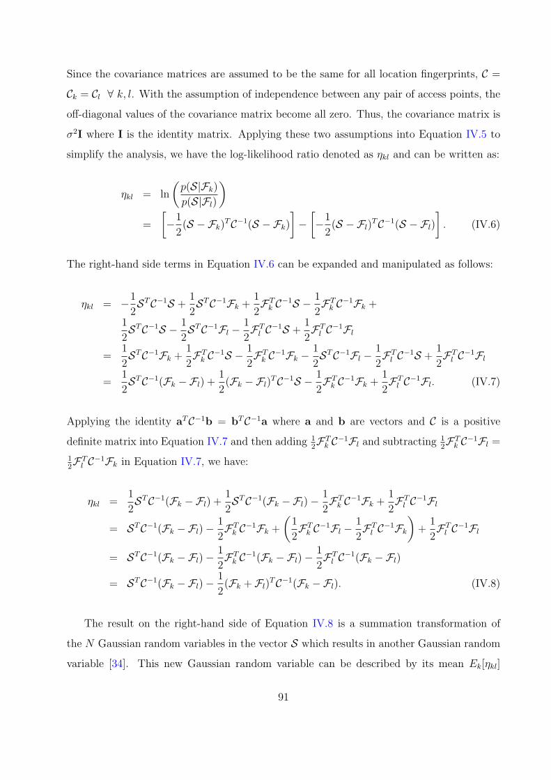
Since the covariance matrices are assumed to be the same for all location fingerprints, C =
Ck = Cl ∀ k, l. With the assumption of independence between any pair of access points, the
off-diagonal values of the covariance matrix become all zero. Thus, the covariance matrix is
σ2I where I is the identity matrix. Applying these two assumptions into Equation IV.5 to
simplify the analysis, we have the log-likelihood ratio denoted as ηkl and can be written as:
ηkl = ln
(p(S|Fk)
p(S|Fl)
)
=
[−1
2(S − Fk)
TC−1(S − Fk)
]−
[−1
2(S − Fl)
TC−1(S − Fl)
]. (IV.6)
The right-hand side terms in Equation IV.6 can be expanded and manipulated as follows:
ηkl = −1
2STC−1S +
1
2STC−1Fk +
1
2FT
k C−1S − 1
2FT
k C−1Fk +
1
2STC−1S − 1
2STC−1Fl − 1
2FT
l C−1S +1
2FT
l C−1Fl
=1
2STC−1Fk +
1
2FT
k C−1S − 1
2FT
k C−1Fk − 1
2STC−1Fl − 1
2FT
l C−1S +1
2FT
l C−1Fl
=1
2STC−1(Fk −Fl) +
1
2(Fk −Fl)
TC−1S − 1
2FT
k C−1Fk +1
2FT
l C−1Fl. (IV.7)
Applying the identity aTC−1b = bTC−1a where a and b are vectors and C is a positive
definite matrix into Equation IV.7 and then adding 12FT
k C−1Fl and subtracting 12FT
k C−1Fl =
12FT
l C−1Fk in Equation IV.7, we have:
ηkl =1
2STC−1(Fk −Fl) +
1
2STC−1(Fk −Fl)− 1
2FT
k C−1Fk +1
2FT
l C−1Fl
= STC−1(Fk −Fl)− 1
2FT
k C−1Fk +
(1
2FT
k C−1Fl − 1
2FT
l C−1Fk
)+
1
2FT
l C−1Fl
= STC−1(Fk −Fl)− 1
2FT
k C−1(Fk −Fl)− 1
2FT
l C−1(Fk −Fl)
= STC−1(Fk −Fl)− 1
2(Fk + Fl)
TC−1(Fk −Fl). (IV.8)
The result on the right-hand side of Equation IV.8 is a summation transformation of
the N Gaussian random variables in the vector S which results in another Gaussian random
variable [34]. This new Gaussian random variable can be described by its mean Ek[ηkl]
91
and its variance V ark[ηkl] with respect to the location fingerprint Fk. The mean of the
log-likelihood ratio is [34]:
Ek[ηkl] = Ek[ST ]C−1(Fk −Fl)− 1
2(Fk + Fl)
TC−1(Fk −Fl)
= FTk C−1(Fk −Fl)− 1
2(Fk + Fl)
TC−1(Fk −Fl)
=1
2(Fk −Fl)
TC−1(Fk −Fl). (IV.9)
The variance of the log-likelihood ratio is [34]:
V ark[ηkl] = Ek[(ηkl − Ek[ηkl])2]
= Ek[(STC−1(Fk −Fl)−FT
k C−1(Fk −Fl))2
]
= Ek[(S − Fk)TC−1(Fk −Fl)(S − Fk)
TC−1(Fk −Fl)]
= Ek[(Fk −Fl)TC−1(S − Fk)(S − Fk)
TC−1(Fk −Fl)]
= (Fk −Fl)TC−1(Fk −Fl). (IV.10)
Note that the last line is the result of the covariance matrix expression which is C = Ek[(S −Fk)(S−Fk)
T ]. The common term (Fk−Fl)TC−1(Fk−Fl) in both the mean and the variance is
similar to Equation II.6 described in Chapter II. This term is called the Mahalanobis distance
between the two densities of the location fingerprints p(S|Fk) and p(S|Fl). If we denote the
Mahalanobis distance as Hkl = (Fk − Fl)TC−1(Fk − Fl), the mean and the variance of the
log-likelihood ratio ηkl when the pattern S corresponds to the location fingerprint Fk are [34]:
Ek[ηkl] =1
2Hkl, and (IV.11)
V ark[ηkl] = Hkl. (IV.12)
The total probability of error for a two-location system can be derived from two condi-
tional distributions that compare between log-likelihood ratio ηkl and the logarithm of the
threshold denoted as γ = ln(
p(Fl)p(Fk)
). First, the distribution of p(ηkl > γ|Fk) isN (
12Hkl, Hkl
))
when the sample RSS vector S comes from fingerprint Fk [34]. Second, the distribution of
92
p(ηkl < γ|Fl) is N (−12Hkl, Hkl
)) when the sample RSS vector S comes from fingerprint
Fl [34]. These two probabilities can be calculated as:
p(ηkl > γ|Fk) =
∫ ∞
γ
1√2πHkl
exp
[−(ηkl + 1
2Hkl)
2
2Hkl
]
= 1− Φ
(γ + 1
2Hkl√
Hkl
), (IV.13)
and
p(ηkl < γ|Fl) =
∫ γ
−∞
1√2πHkl
exp
[−(ηkl − 1
2Hkl)
2
2Hkl
]
= Φ
(γ − 1
2Hkl√
Hkl
), (IV.14)
where Φ is defined as:
Φ(η) =
∫ η
−∞
1√2π
exp(−y2
2)dy. (IV.15)
Substituting the results from Equation IV.13 and Equation IV.14 into Equation IV.2, we
have:
Pc = 1− Pe = 1− p(Fk)Φ
(γ − 1
2Hkl√
Hkl
)+ p(Fl)
[1− Φ
(γ + 1
2Hkl√
Hkl
)]. (IV.16)
When assuming that a priori probabilities are equal for every location p(Fk) = p(Fl), ∀ k, l,
the logarithm of the threshold γ = ln( p(Fl)p(Fk)
) = ln(1) becomes zero and for the two-location
system p(Fk) = p(Fl) = 12. The probability of returning the correct location can be calcu-
lated by:
Pc = 1−Pe = 1− 1
2Φ
(−1
2
√Hkl
)− 1
2
[1− Φ
(1
2
√Hkl
)](IV.17)
For a positioning system with more than two locations, the positioning algorithm based
on the probabilistic approach has to calculate the discriminant function according to the
Bayes’s decision rule for all location fingerprints: dl(S) = p(S|Fl)p(Fl), l = 1, 2, . . . ,M.
By taking the natural logarithm of this decision function and substituting Equation IV.4
into the decision function, we have a decision function that minimizes the average cost of
missclassification:
dl(S) = ln p(Fl)− N
2ln 2π − 1
2ln |C| − 1
2
[(S − Fl)
TC−1(S − Fl)]
(IV.18)
93
Since we assume that all locations are equally likely, the a priori probabilities p(Fl) are equal
and can be dropped from consideration. Moreover, the second and the third terms on the
right-hand side of Equation IV.18 do not depend on the location in this model and they can
be dropped from our consideration. The last term is the Mahalanobis distance between a
sample pattern and a location fingerprint that is used to determine the estimated location.
Dl(S) =[(S − Fl)
TC−1(S − Fl)]
(IV.19)
This result indicates that the Mahalanobis distance could be used as an alternative to the
Euclidean distance to determine the location in indoor positioning systems. The improve-
ment provided by the Mahalanobis distance lies in its use of the covariance matrix to adjust
the distance metric. Thus far, the Mahalanobis distance has not been used by any indoor po-
sitioning systems based on location fingerprint technique. We will show in the next chapter
that the Mahalanobis distance can be used to improve the performance of indoor positioning
systems.
2. Euclidean Distance with Lognormal Assumption and Identity Covariance
The above analysis of the probability of returning the correct location degenerates into
the Euclidean distance based system when identity covariance matrices are assumed for
all location fingerprints. Given a location fingerprint vector Fl = [ρ1, ρ2, . . . , ρN ]T for l =
1, 2, . . . , L where L is the total number of locations, a sample RSS vector S = [s1, s2, . . . , sN ]T ,
and the identity covariance matrix C = I(N×N), Equation IV.19 is reduced to the square of
Euclidean distance:
D2E,l(S) =
[(S − Fl)
T I−1(S − Fl)]
= ([s1, s2, . . . , sN ]− [ρ1, ρ2, . . . , ρN ])× ([s1, s2, . . . , sN ]− [ρ1, ρ2, . . . , ρN ])T
=N∑
i=1
(si − ρi)2 =
N∑i=1
q2i . (IV.20)
The smallest such distance among all locations is used to indicate the estimated location by
the positioning algorithm.
94
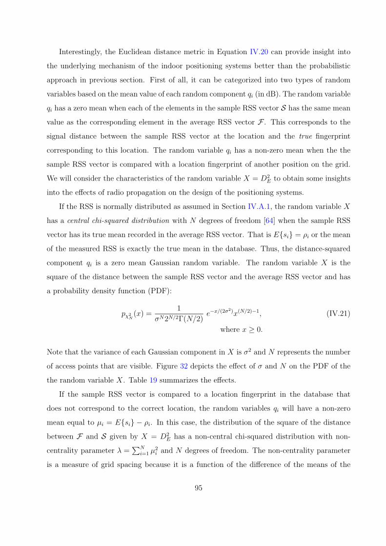
Interestingly, the Euclidean distance metric in Equation IV.20 can provide insight into
the underlying mechanism of the indoor positioning systems better than the probabilistic
approach in previous section. First of all, it can be categorized into two types of random
variables based on the mean value of each random component qi (in dB). The random variable
qi has a zero mean when each of the elements in the sample RSS vector S has the same mean
value as the corresponding element in the average RSS vector F . This corresponds to the
signal distance between the sample RSS vector at the location and the true fingerprint
corresponding to this location. The random variable qi has a non-zero mean when the the
sample RSS vector is compared with a location fingerprint of another position on the grid.
We will consider the characteristics of the random variable X = D2E to obtain some insights
into the effects of radio propagation on the design of the positioning systems.
If the RSS is normally distributed as assumed in Section IV.A.1, the random variable X
has a central chi-squared distribution with N degrees of freedom [64] when the sample RSS
vector has its true mean recorded in the average RSS vector. That is E{si} = ρi or the mean
of the measured RSS is exactly the true mean in the database. Thus, the distance-squared
component qi is a zero mean Gaussian random variable. The random variable X is the
square of the distance between the sample RSS vector and the average RSS vector and has
a probability density function (PDF):
pχ2N(x) =
1
σN2N/2Γ(N/2)e−x/(2σ2)x(N/2)−1, (IV.21)
where x ≥ 0.
Note that the variance of each Gaussian component in X is σ2 and N represents the number
of access points that are visible. Figure 32 depicts the effect of σ and N on the PDF of the
the random variable X. Table 19 summarizes the effects.
If the sample RSS vector is compared to a location fingerprint in the database that
does not correspond to the correct location, the random variables qi will have a non-zero
mean equal to µi = E{si} − ρi. In this case, the distribution of the square of the distance
between F and S given by X = D2E has a non-central chi-squared distribution with non-
centrality parameter λ =∑N
i=1 µ2i and N degrees of freedom. The non-centrality parameter
is a measure of grid spacing because it is a function of the difference of the means of the
95
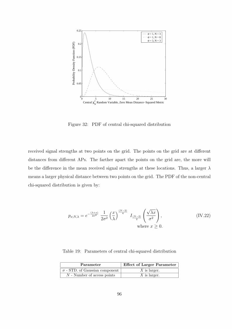
0 5 10 15 20 25 300
0.05
0.1
0.15
0.2
0.25
Central χN2 Random Variable, Zero Mean Distance−Squared Metric
Pro
babi
lity
Den
sity
Fun
ctio
n (P
DF
)
σ = 1, N = 3σ = 1, N = 8σ = 3, N = 3
Figure 32: PDF of central chi-squared distribution
received signal strengths at two points on the grid. The points on the grid are at different
distances from different APs. The farther apart the points on the grid are, the more will
be the difference in the mean received signal strengths at these locations. Thus, a larger λ
means a larger physical distance between two points on the grid. The PDF of the non-central
chi-squared distribution is given by:
px;N,λ = e−(λ+x)
2σ21
2σ2
(x
λ
) (N−2)4
I (N−2)2
(√λx
σ2
), (IV.22)
where x ≥ 0.
Table 19: Parameters of central chi-squared distribution
Parameter Effect of Larger Parameterσ - STD. of Gaussian component X is larger.
N - Number of access points X is larger.
96
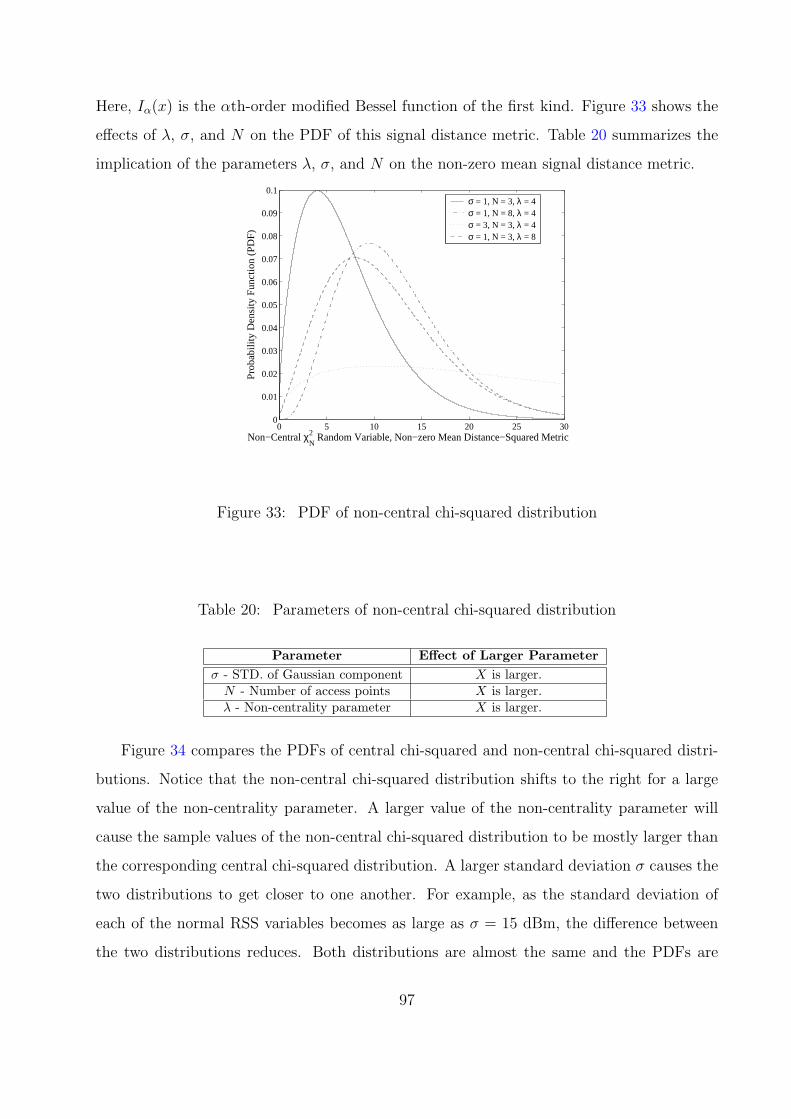
Here, Iα(x) is the αth-order modified Bessel function of the first kind. Figure 33 shows the
effects of λ, σ, and N on the PDF of this signal distance metric. Table 20 summarizes the
implication of the parameters λ, σ, and N on the non-zero mean signal distance metric.
0 5 10 15 20 25 300
0.01
0.02
0.03
0.04
0.05
0.06
0.07
0.08
0.09
0.1
Non−Central χN2 Random Variable, Non−zero Mean Distance−Squared Metric
Pro
ba
bili
ty D
en
sity
Fu
nct
ion
(P
DF
)
σ = 1, N = 3, λ = 4σ = 1, N = 8, λ = 4σ = 3, N = 3, λ = 4σ = 1, N = 3, λ = 8
Figure 33: PDF of non-central chi-squared distribution
Table 20: Parameters of non-central chi-squared distribution
Parameter Effect of Larger Parameterσ - STD. of Gaussian component X is larger.
N - Number of access points X is larger.λ - Non-centrality parameter X is larger.
Figure 34 compares the PDFs of central chi-squared and non-central chi-squared distri-
butions. Notice that the non-central chi-squared distribution shifts to the right for a large
value of the non-centrality parameter. A larger value of the non-centrality parameter will
cause the sample values of the non-central chi-squared distribution to be mostly larger than
the corresponding central chi-squared distribution. A larger standard deviation σ causes the
two distributions to get closer to one another. For example, as the standard deviation of
each of the normal RSS variables becomes as large as σ = 15 dBm, the difference between
the two distributions reduces. Both distributions are almost the same and the PDFs are
97
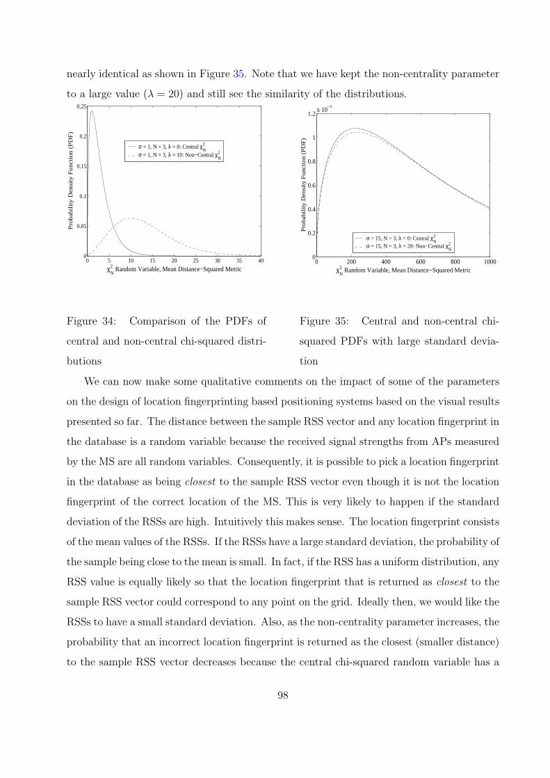
nearly identical as shown in Figure 35. Note that we have kept the non-centrality parameter
to a large value (λ = 20) and still see the similarity of the distributions.
0 5 10 15 20 25 30 35 400
0.05
0.1
0.15
0.2
0.25
χN2 Random Variable, Mean Distance−Squared Metric
Pro
ba
bili
ty D
en
sity
Fu
nct
ion
(P
DF
)
σ = 1, N = 3, λ = 0: Central χN2
σ = 1, N = 3, λ = 10: Non−Central χN2
Figure 34: Comparison of the PDFs of
central and non-central chi-squared distri-
butions
0 200 400 600 800 10000
0.2
0.4
0.6
0.8
1
1.2x 10
−3
χN2 Random Variable, Mean Distance−Squared Metric
Pro
ba
bili
ty D
en
sity
Fu
nct
ion
(P
DF
)
σ = 15, N = 3, λ = 0: Central χN2
σ = 15, N = 3, λ = 20: Non−Central χN2
Figure 35: Central and non-central chi-
squared PDFs with large standard devia-
tion
We can now make some qualitative comments on the impact of some of the parameters
on the design of location fingerprinting based positioning systems based on the visual results
presented so far. The distance between the sample RSS vector and any location fingerprint in
the database is a random variable because the received signal strengths from APs measured
by the MS are all random variables. Consequently, it is possible to pick a location fingerprint
in the database as being closest to the sample RSS vector even though it is not the location
fingerprint of the correct location of the MS. This is very likely to happen if the standard
deviation of the RSSs are high. Intuitively this makes sense. The location fingerprint consists
of the mean values of the RSSs. If the RSSs have a large standard deviation, the probability of
the sample being close to the mean is small. In fact, if the RSS has a uniform distribution, any
RSS value is equally likely so that the location fingerprint that is returned as closest to the
sample RSS vector could correspond to any point on the grid. Ideally then, we would like the
RSSs to have a small standard deviation. Also, as the non-centrality parameter increases, the
probability that an incorrect location fingerprint is returned as the closest (smaller distance)
to the sample RSS vector decreases because the central chi-squared random variable has a
98
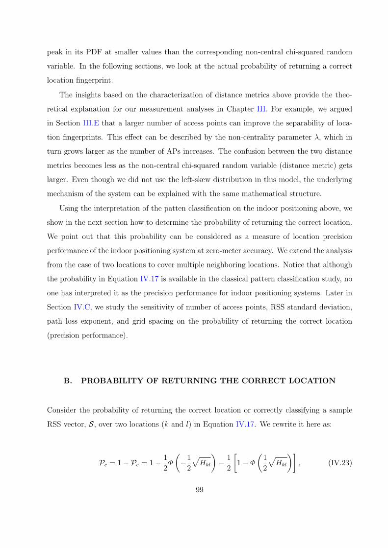
peak in its PDF at smaller values than the corresponding non-central chi-squared random
variable. In the following sections, we look at the actual probability of returning a correct
location fingerprint.
The insights based on the characterization of distance metrics above provide the theo-
retical explanation for our measurement analyses in Chapter III. For example, we argued
in Section III.E that a larger number of access points can improve the separability of loca-
tion fingerprints. This effect can be described by the non-centrality parameter λ, which in
turn grows larger as the number of APs increases. The confusion between the two distance
metrics becomes less as the non-central chi-squared random variable (distance metric) gets
larger. Even though we did not use the left-skew distribution in this model, the underlying
mechanism of the system can be explained with the same mathematical structure.
Using the interpretation of the patten classification on the indoor positioning above, we
show in the next section how to determine the probability of returning the correct location.
We point out that this probability can be considered as a measure of location precision
performance of the indoor positioning system at zero-meter accuracy. We extend the analysis
from the case of two locations to cover multiple neighboring locations. Notice that although
the probability in Equation IV.17 is available in the classical pattern classification study, no
one has interpreted it as the precision performance for indoor positioning systems. Later in
Section IV.C, we study the sensitivity of number of access points, RSS standard deviation,
path loss exponent, and grid spacing on the probability of returning the correct location
(precision performance).
B. PROBABILITY OF RETURNING THE CORRECT LOCATION
Consider the probability of returning the correct location or correctly classifying a sample
RSS vector, S, over two locations (k and l) in Equation IV.17. We rewrite it here as:
Pc = 1−Pe = 1− 1
2Φ
(−1
2
√Hkl
)− 1
2
[1− Φ
(1
2
√Hkl
)], (IV.23)
99
where, Hkl = (Fk − Fl)TC−1(Fk − Fl) is the Mahalanobis distance between the two distri-
bution of location fingerprint Fk and Fl. The relationship between the probability Pc and
the Mahalanobis distance is plotted in Figure 36. We can see that the performance improve-
ment of classification is very significant for the Mahalanobis distance between 1 and 11. To
maintain a high precision performance for any indoor positioning system, we need to ensure
that the Mahalanobis distance between any two location fingerprints is as large as possible.
0 2 4 6 8 10 12 14 16 18 200.55
0.6
0.65
0.7
0.75
0.8
0.85
0.9
0.95
1
Mahalanobis Distance in Signal Space (Hkl
)
Pro
babi
lity
of R
etur
ning
the
Cor
rect
Loc
atio
n (P
c)
Figure 36: Effect of Mahalanobis distance on probability
We observe that the calculation of the probability does not depend on the sample RSS
vector S at all. Only the mean vectors and the covariance matrix are needed. It is obvious
that the separation of location fingerprints (mean vectors) and the magnitude of variance
of the RSS (or standard deviation of RSS) are the two main factors that dominate the
performance of indoor positioning systems. To improve the accuracy performance, we would
like to have the mean vectors located as far apart as possible in the signal space and have
the magnitude of the variance to be as small as possible. However, to gain detailed insight
on how to improve the precision performance, we consider an alternative calculation of the
the precision performance in the next subsection. The results of Equation IV.17 and the
100
alternative calculation are extended to describe the positioning system with more than two
locations in Section IV.B.2.
1. Alternate Calculation of Probability with the Euclidean Distance
Here we present an alternative approach to interpret and calculate the probability of return-
ing the correct location. With this alternative interpretation, it is more obvious than the
probabilistic approach, how the number of access points will affect the system performance.
The analysis here provides more insight to better improve the precision performance. The
derivation of the probability is based on the use of two chi-squared distance metrics discussed
in Section IV.A.2.
Although it is tempting to directly compare the central chi-squared random variable to
the non-central chi-squared random variable, we cannot do so directly due to the dependency
of the two random variables which are transformations of the same random vector S (the
sample RSS vector). However, we can perform the following analysis to determine the
probability of returning the correct fingerprint as the estimate of the location when a MS
reports a sample RSS vector.
Let A be the square of the distance between the sample RSS vector S = (s1, s2, ..., sN)T
and the average RSS vector of the true location F = (ρ1, ρ2, ..., ρN)T . Let B be the
square of the distance between the sample RSS vector S and the location fingerprint F ′ =
(ρ′1, ρ′2, .., ρ
′N)T of a neighboring point on the grid. We then denote {A < B} = {A ≤ B}
as the event that the distance between the sample RSS vector and the correct location
fingerprint is smaller than the distance between the sample RSS vector and the incorrect
neighboring location fingerprint. We can determine the probability of this event. Firstly, we
evaluate {A ≤ B} as follows:
A ≤ B
⇒N∑
i=1
(si − ρi)2 ≤
N∑i=1
(si − ρ′i)2
⇒N∑
i=1
(si − ρi)2 −
N∑i=1
(si − ρ′i)2 ≤ 0
101
⇒N∑
i=1
(s2i − 2siρi + ρ2
i )−N∑
i=1
(s2i − 2siρ
′i + ρ
′2i ) ≤ 0
⇒ 2N∑
i=1
si(ρ′i − ρi) +
N∑i=1
(ρ2i − ρ
′2i ) ≤ 0
⇒ 2N∑
i=1
siβi +N∑
i=1
Γi ≤ 0, (IV.24)
where Γi = (ρ2i − ρ
′2i ) and βi = (ρ′i − ρi).
To determine the probability of the event in Equation IV.24, we first apply the properties
of the sum of multiple independent Gaussian random variables [65]. The left-hand side of
Equation IV.24, θ = 2∑N
i=1 siβi +∑N
i=1 Γi, is a new Gaussian random variable when all si
are Gaussian. The random variable θ has following mean and variance
µθ = 2N∑
i=1
ρiβi +N∑
i=1
Γi,
σ2θ =
N∑i=1
(2βiσi)2. (IV.25)
Therefore, the probability that the system returns the correct location when it compares
just two location fingerprints to the sample RSS vector is given by:
Pr{θ ≤ 0} =
∫ 0
−∞
1√2πσθ
e− (θ−µθ)2
2σ2θ dθ
=1
2
2√π
∫ − µθ√2σθ
−∞e−t2dt
=1
2+
1
2erf
( −µθ√2σθ
). (IV.26)
Note that the result in Equation IV.26 is equivalent to the result of Equation IV.17 and is
a special case of Equation IV.16. Our mathematical analysis described thus far does not
explain why the probabilistic approach is better than the Euclidean distance approach as
concluded in the literature. The superiority of the probabilistic approach as discussed in
Chapter II is due to its ability to capture the actual distribution of RSS. In this model, we
assume a simplified mathematical model of Gaussian distribution; thus, the benefit of the
real distribution is not present.
102
From Equation IV.25 and Equation IV.26, we observe that the mean and variance of the
new distribution are influenced by two parameters of the positioning system: the number
of access points N and the standard deviation σi of the normally distributed RSS variables.
This insight provide more details than the one given previously by Equation IV.17. The
parameters βi and Γi do not have any explicit meaning but are related to the non-centrality
parameter λ discussed earlier. That is, they both depend on the difference between the
mean RSS at the two locations that is determined by the path loss of the signal. In turn,
the path loss of the signal depends on the site and the physical distances of the locations
from the N access points and indirectly to the physical distance between the locations. As
observed in Chapter III, in certain location area with NLOS the path loss exponent is quite
large, small physical distance separation between any two locations will result in large mean
RSS vector separation in signal space. This observation suggests that in a large path loss
exponent environment the positioning system can operate with better precision. We evaluate
the effects of these parameters (N and σ) together with the grid spacing (g) and the path
loss exponent (α) on the precision performance in Section IV.C.
2. Extension to Multi-Location Systems
In a real positioning system, the database contains several entries depending on the size of
the office floor and the grid spacing. The positioning system makes comparisons between
the sample RSS vector and all of these location fingerprints. The database may be arranged
hierarchically. In the first phase, the APs seen by the MS are matched. Then the location
fingerprints corresponding to these APs alone are compared with the sample RSS vector. In
any case, each comparison depends on the same sample RSS vector. Therefore, to be able
to calculate the probability of returning a correct location, we will need to know the joint
probability density function (PDF) of all random variables of the form p(S|F1,F2, . . . ,Fl)
for subsituting in Equation IV.1 or the complex form of θ in Equation IV.26. Deriving an
analytical model can be quite cumbersome where there may be tens or hundreds of location
fingerprints being compared.
To simplify our analysis, we consider a model with only a simple approximation of the
103
probability of returning the correct location system. Without loss of generality, we use the
Euclidean distance approach for our explanation. The result described next is applicable to
the probabilistic approach since the calculation of the probability of returning the correct
location in Equation IV.17 and Equation IV.26 are equivalent.
Let θk =∑N
i=1(si − ρi)2 − ∑N
i=1(si − ρ′k,i)2 be the comparison variable. The variable
θk compares the distance between the sample RSS vector S and (a) the correct location
fingerprint F and (b) the k-th incorrect location fingerprint F ′k. The index k runs from 1 to
K excluding the correct location denoted by the index c. The variable K corresponds to the
number of entries in the database. Then, we can write the probability of correct decision as:
Prob{Correct Estimation} = Pc
= P {θ1 ≤ 0, · · · , θc−1 ≤ 0, θc+1 ≤ 0, · · · , θK ≤ 0} (IV.27)
Under the assumptions stated in Section IV.A, the sampled RSS vector can be viewed as a
fingerprint vector that has Gaussian noise adding to it around the mean of each RSS element.
This is analogous to a signal constellation used in traditional digital signal modulation
representation. To compute this probability, we need the joint distribution of the random
variables θk. Alternatively, we can evaluate an approximation to the probability of returning
a correct location Pc by using the union bound technique [66]. In this case, the RSS elements
from multiple access points may not form a regular grid. We can also not represent them
in only two dimensions like Quadrature Amplitude Modulation (QAM). Determining the
union bound becomes cumbersome as well. To avoid the cumbersome calculation of the
joint distribution or union bound, we make the assumption that they are independent. In
such a case:
Prob{Correct Estimation} = Pc =K∏
k=1k 6=c
Pr{θk ≤ 0}. (IV.28)
Equation IV.28 is an approximation to the probability of returning the correct location for
an indoor location system when the correct position is c and there are K location fingerprint
entries in the database. While this assumption is not correct, we compare the results of this
assumption with simulation results to see how close the results are. As we shall see, the
assumption of independence provides a reasonable approximation.
104
When there are a large number of locations or K is large, a simpler approximation can
be calculated with the Pr{θk ≤ 0} of the nearest neighboring fingerprints of any correct
location. For a 2-D grid of positions, the largest number of nearest neighbor fingerprints is
eight. Assuming that the set of nearest neighboring fingerprints is denoted as Mn, The Pc
and Pe can be approximated as:
Pc ≈∏
j∈Mn
Pr{θj ≤ 0}, and (IV.29)
Pe ≈ 1−∏
j∈Mn
Pr{θj ≤ 0}. (IV.30)
C. PERFORMANCE EVALUATION
The major performance metrics of interest for indoor positioning systems are the accuracy
and the precision in estimating a location. In this section, we investigate how the path
loss and RSS characteristics influence the precision. As a measure of precision at zero-
meter accuracy, we look at the probability of making a correct estimation of the location.
A better measure of accuracy and precision is the distribution of the error in the location
estimate which will be presented in Section IV.D. We use Equation IV.28 as the analytical
approximation of the measure of precision and also compare this with simulations. We use
a simple grid in this work as described below.
1. System Model Setup
Figure 37 illustrates an indoor positioning system with L2 = 25 points on the grid. The
grid at the center is labeled with a ? and is assumed to be the current position of the
mobile station reporting the sample RSS vector. The neighboring positions with location
fingerprints recorded in the database during the site-survey are labeled with ◦. There are 8
neighboring positions in this system. The total number of positions within this system and
in the database is K = 9. The outer most positions are labeled with 2 and reserved for
placing access points only.
105
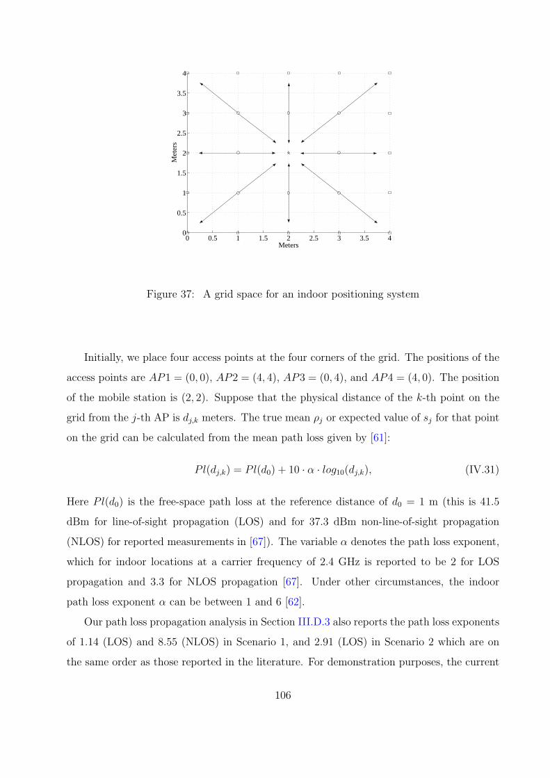
0 0.5 1 1.5 2 2.5 3 3.5 40
0.5
1
1.5
2
2.5
3
3.5
4
Meters
Met
ers
Figure 37: A grid space for an indoor positioning system
Initially, we place four access points at the four corners of the grid. The positions of the
access points are AP1 = (0, 0), AP2 = (4, 4), AP3 = (0, 4), and AP4 = (4, 0). The position
of the mobile station is (2, 2). Suppose that the physical distance of the k-th point on the
grid from the j-th AP is dj,k meters. The true mean ρj or expected value of sj for that point
on the grid can be calculated from the mean path loss given by [61]:
Pl(dj,k) = Pl(d0) + 10 · α · log10(dj,k), (IV.31)
Here Pl(d0) is the free-space path loss at the reference distance of d0 = 1 m (this is 41.5
dBm for line-of-sight propagation (LOS) and for 37.3 dBm non-line-of-sight propagation
(NLOS) for reported measurements in [67]). The variable α denotes the path loss exponent,
which for indoor locations at a carrier frequency of 2.4 GHz is reported to be 2 for LOS
propagation and 3.3 for NLOS propagation [67]. Under other circumstances, the indoor
path loss exponent α can be between 1 and 6 [62].
Our path loss propagation analysis in Section III.D.3 also reports the path loss exponents
of 1.14 (LOS) and 8.55 (NLOS) in Scenario 1, and 2.91 (LOS) in Scenario 2 which are on
the same order as those reported in the literature. For demonstration purposes, the current
106
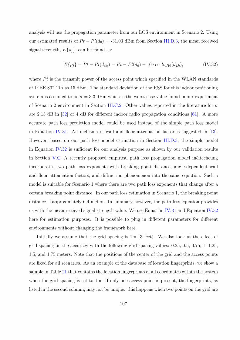
analysis will use the propagation parameter from our LOS environment in Scenario 2. Using
our estimated results of Pt− Pl(d0) = -31.03 dBm from Section III.D.3, the mean received
signal strength, E{ρj}, can be found as:
E{ρj} = Pt− Pl(dj,k) = Pt− Pl(d0)− 10 · α · log10(dj,k), (IV.32)
where Pt is the transmit power of the access point which specified in the WLAN standards
of IEEE 802.11b as 15 dBm. The standard deviation of the RSS for this indoor positioning
system is assumed to be σ = 3.3 dBm which is the worst case value found in our experiment
of Scenario 2 environment in Section III.C.2. Other values reported in the literature for σ
are 2.13 dB in [32] or 4 dB for different indoor radio propagation conditions [61]. A more
accurate path loss prediction model could be used instead of the simple path loss model
in Equation IV.31. An inclusion of wall and floor attenuation factor is suggested in [13].
However, based on our path loss model estimation in Section III.D.3, the simple model
in Equation IV.32 is sufficient for our analysis purpose as shown by our validation results
in Section V.C. A recently proposed empirical path loss propagation model inc̃itecheung
incorporates two path loss exponents with breaking point distance, angle-dependent wall
and floor attenuation factors, and diffraction phenomenon into the same equation. Such a
model is suitable for Scenario 1 where there are two path loss exponents that change after a
certain breaking point distance. In our path loss estimation in Scenario 1, the breaking point
distance is approximately 6.4 meters. In summary however, the path loss equation provides
us with the mean received signal strength value. We use Equation IV.31 and Equation IV.32
here for estimation purposes. It is possible to plug in different parameters for different
environments without changing the framework here.
Initially we assume that the grid spacing is 1m (3 feet). We also look at the effect of
grid spacing on the accuracy with the following grid spacing values: 0.25, 0.5, 0.75, 1, 1.25,
1.5, and 1.75 meters. Note that the positions of the center of the grid and the access points
are fixed for all scenarios. As an example of the database of location fingerprints, we show a
sample in Table 21 that contains the location fingerprints of all coordinates within the system
when the grid spacing is set to 1m. If only one access point is present, the fingerprints, as
listed in the second column, may not be unique. this happens when two points on the grid are
107
at the same distance from the access point. Additional access points make the fingerprints
unique.
Table 21: RSS fingerprints of indoor location
Access Point AP1 (dBm) AP2 (dBm) AP3 (dBm) AP4 (dBm)Coordinate (0,0) (4,4) (0,4) (4,0)
(2,2) -44.1700 -44.1700 -44.1700 -44.1700(1,1) -35.4100 -49.2942 -45.5800 -45.5800(1,2) -41.2000 -47.2379 -41.2000 -47.2379(1,3) -45.5800 -45.5800 -35.4100 -49.2942(2,1) -41.2000 -47.2379 -47.2379 -41.2000(2,3) -47.2379 -41.2000 -41.2000 -47.2379(3,1) -45.5800 -45.5800 -49.2942 -35.4100(3,2) -47.2379 -41.2000 -47.2379 -41.2000(3,3) -49.2942 -35.4100 -45.5800 -45.5800
2. Results of the Probability of Returning the Correct Location for a Single
Neighbor
Based on the model above, we calculate the precision at zero-meter accuracy in terms of
the probability of returning the correct position. Initially we consider only one neighboring
point on the grid (we compare the location fingerprints at the positions (2,2) and (2,1)). For
this, we can simply use the analytical expression from Equation IV.26.
We first look at the impact of the number of access points deployed by varying this
number from one to 16 according to the system in Figure 37. The first four access points
are installed at the four corners and the rest are located at the following coordinates: AP5
= (2,0), AP6 = (4,2), AP7 = (2,4), AP8 = (0,2), AP9 = (1,0), AP10 = (4,1), AP11
= (3,4), AP12 = (0,3), AP13 = (3,0), AP14 = (4,3), AP15 = (1,4), and AP16 = (0,1).
Figure 38 shows the results of using Equation IV.26 when the number of access points
increases. The label “Ana” indicates calculation from the analytical equations discussed
earlier. A higher number of access points improves the precision but the probability does
not increase significantly for N > 5. We also see that a larger standard deviation of the
RSS results in poorer precision especially for a smaller number of APs. For instance, if the
standard deviation of the RSS changes from 1 to 4, the probability of returning the correct
108
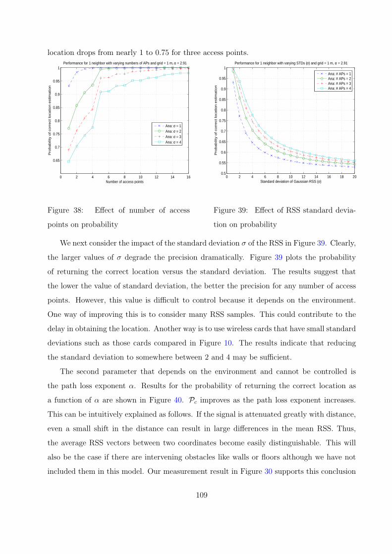
location drops from nearly 1 to 0.75 for three access points.
0 2 4 6 8 10 12 14 16
0.65
0.7
0.75
0.8
0.85
0.9
0.95
1
Number of access points
Pro
babili
ty o
f co
rrect
loca
tion
est
ima
tion
Performance for 1 neighbor with varying numbers of APs and grid = 1 m, α = 2.91
Ana: σ = 1Ana: σ = 2Ana: σ = 3Ana: σ = 4
Figure 38: Effect of number of access
points on probability
0 2 4 6 8 10 12 14 16 18 200.5
0.55
0.6
0.65
0.7
0.75
0.8
0.85
0.9
0.95
1
Standard deviation of Gaussian RSS (σ)
Pro
bab
ility
of co
rrect
loca
tion
est
imatio
n
Performance for 1 neighbor with varying STDs (σ) and grid = 1 m, α = 2.91
Ana: # APs = 1Ana: # APs = 2Ana: # APs = 3Ana: # APs = 4
Figure 39: Effect of RSS standard devia-
tion on probability
We next consider the impact of the standard deviation σ of the RSS in Figure 39. Clearly,
the larger values of σ degrade the precision dramatically. Figure 39 plots the probability
of returning the correct location versus the standard deviation. The results suggest that
the lower the value of standard deviation, the better the precision for any number of access
points. However, this value is difficult to control because it depends on the environment.
One way of improving this is to consider many RSS samples. This could contribute to the
delay in obtaining the location. Another way is to use wireless cards that have small standard
deviations such as those cards compared in Figure 10. The results indicate that reducing
the standard deviation to somewhere between 2 and 4 may be sufficient.
The second parameter that depends on the environment and cannot be controlled is
the path loss exponent α. Results for the probability of returning the correct location as
a function of α are shown in Figure 40. Pc improves as the path loss exponent increases.
This can be intuitively explained as follows. If the signal is attenuated greatly with distance,
even a small shift in the distance can result in large differences in the mean RSS. Thus,
the average RSS vectors between two coordinates become easily distinguishable. This will
also be the case if there are intervening obstacles like walls or floors although we have not
included them in this model. Our measurement result in Figure 30 supports this conclusion
109
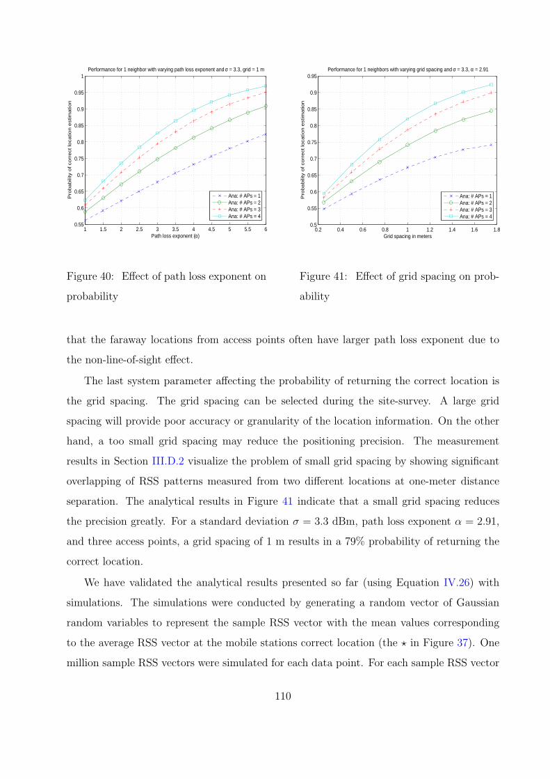
1 1.5 2 2.5 3 3.5 4 4.5 5 5.5 60.55
0.6
0.65
0.7
0.75
0.8
0.85
0.9
0.95
1
Path loss exponent (α)
Pro
babili
ty o
f co
rrect
loca
tion e
stim
atio
nPerformance for 1 neighbor with varying path loss exponent and σ = 3.3, grid = 1 m
Ana: # APs = 1Ana: # APs = 2Ana: # APs = 3Ana: # APs = 4
Figure 40: Effect of path loss exponent on
probability
0.2 0.4 0.6 0.8 1 1.2 1.4 1.6 1.80.5
0.55
0.6
0.65
0.7
0.75
0.8
0.85
0.9
0.95
Grid spacing in meters
Pro
ba
bili
ty o
f co
rre
ct lo
catio
n e
stim
atio
n
Performance for 1 neighbors with varying grid spacing and σ = 3.3, α = 2.91
Ana: # APs = 1Ana: # APs = 2Ana: # APs = 3Ana: # APs = 4
Figure 41: Effect of grid spacing on prob-
ability
that the faraway locations from access points often have larger path loss exponent due to
the non-line-of-sight effect.
The last system parameter affecting the probability of returning the correct location is
the grid spacing. The grid spacing can be selected during the site-survey. A large grid
spacing will provide poor accuracy or granularity of the location information. On the other
hand, a too small grid spacing may reduce the positioning precision. The measurement
results in Section III.D.2 visualize the problem of small grid spacing by showing significant
overlapping of RSS patterns measured from two different locations at one-meter distance
separation. The analytical results in Figure 41 indicate that a small grid spacing reduces
the precision greatly. For a standard deviation σ = 3.3 dBm, path loss exponent α = 2.91,
and three access points, a grid spacing of 1 m results in a 79% probability of returning the
correct location.
We have validated the analytical results presented so far (using Equation IV.26) with
simulations. The simulations were conducted by generating a random vector of Gaussian
random variables to represent the sample RSS vector with the mean values corresponding
to the average RSS vector at the mobile stations correct location (the ? in Figure 37). One
million sample RSS vectors were simulated for each data point. For each sample RSS vector
110
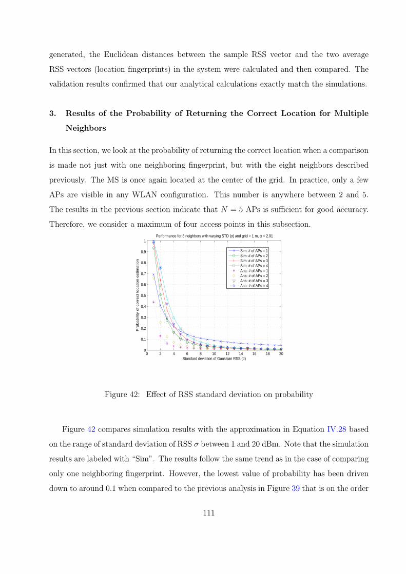
generated, the Euclidean distances between the sample RSS vector and the two average
RSS vectors (location fingerprints) in the system were calculated and then compared. The
validation results confirmed that our analytical calculations exactly match the simulations.
3. Results of the Probability of Returning the Correct Location for Multiple
Neighbors
In this section, we look at the probability of returning the correct location when a comparison
is made not just with one neighboring fingerprint, but with the eight neighbors described
previously. The MS is once again located at the center of the grid. In practice, only a few
APs are visible in any WLAN configuration. This number is anywhere between 2 and 5.
The results in the previous section indicate that N = 5 APs is sufficient for good accuracy.
Therefore, we consider a maximum of four access points in this subsection.
0 2 4 6 8 10 12 14 16 18 200
0.1
0.2
0.3
0.4
0.5
0.6
0.7
0.8
0.9
1Performance for 8 neighbors with varying STD (σ) and grid = 1 m, α = 2.91
Standard deviation of Gaussian RSS (σ)
Pro
babili
ty o
f co
rrect
loca
tion e
stim
atio
n
Sim: # of APs = 1Sim: # of APs = 2Sim: # of APs = 3Sim: # of APs = 4Ana: # of APs = 1Ana: # of APs = 2Ana: # of APs = 3Ana: # of APs = 4
Figure 42: Effect of RSS standard deviation on probability
Figure 42 compares simulation results with the approximation in Equation IV.28 based
on the range of standard deviation of RSS σ between 1 and 20 dBm. Note that the simulation
results are labeled with “Sim”. The results follow the same trend as in the case of comparing
only one neighboring fingerprint. However, the lowest value of probability has been driven
down to around 0.1 when compared to the previous analysis in Figure 39 that is on the order
111
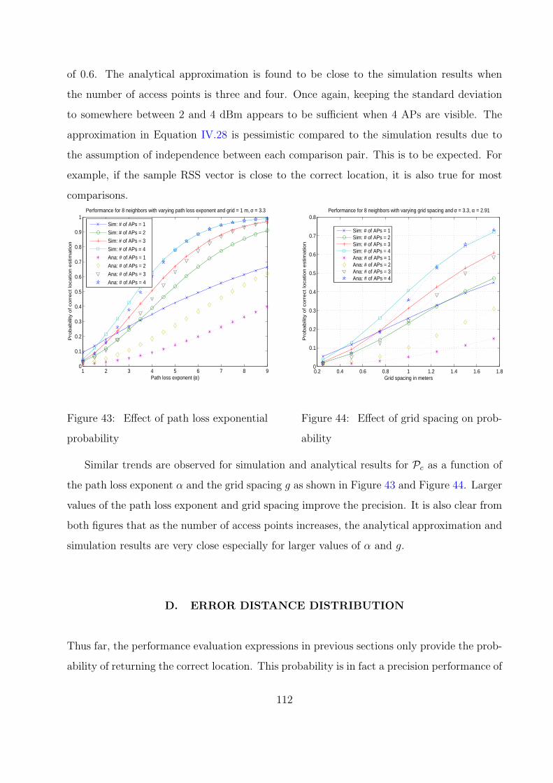
of 0.6. The analytical approximation is found to be close to the simulation results when
the number of access points is three and four. Once again, keeping the standard deviation
to somewhere between 2 and 4 dBm appears to be sufficient when 4 APs are visible. The
approximation in Equation IV.28 is pessimistic compared to the simulation results due to
the assumption of independence between each comparison pair. This is to be expected. For
example, if the sample RSS vector is close to the correct location, it is also true for most
comparisons.
1 2 3 4 5 6 7 8 90
0.1
0.2
0.3
0.4
0.5
0.6
0.7
0.8
0.9
1Performance for 8 neighbors with varying path loss exponent and grid = 1 m, σ = 3.3
Path loss exponent (α)
Pro
bab
ility
of
corr
ect
loca
tion
est
imatio
n
Sim: # of APs = 1
Sim: # of APs = 2
Sim: # of APs = 3
Sim: # of APs = 4
Ana: # of APs = 1
Ana: # of APs = 2
Ana: # of APs = 3
Ana: # of APs = 4
Figure 43: Effect of path loss exponential
probability
0.2 0.4 0.6 0.8 1 1.2 1.4 1.6 1.80
0.1
0.2
0.3
0.4
0.5
0.6
0.7
0.8Performance for 8 neighbors with varying grid spacing and σ = 3.3, α = 2.91
Grid spacing in meters
Pro
ba
bili
ty o
f co
rrect
loca
tion
est
ima
tion
Sim: # of APs = 1Sim: # of APs = 2Sim: # of APs = 3Sim: # of APs = 4Ana: # of APs = 1Ana: # of APs = 2Ana: # of APs = 3Ana: # of APs = 4
Figure 44: Effect of grid spacing on prob-
ability
Similar trends are observed for simulation and analytical results for Pc as a function of
the path loss exponent α and the grid spacing g as shown in Figure 43 and Figure 44. Larger
values of the path loss exponent and grid spacing improve the precision. It is also clear from
both figures that as the number of access points increases, the analytical approximation and
simulation results are very close especially for larger values of α and g.
D. ERROR DISTANCE DISTRIBUTION
Thus far, the performance evaluation expressions in previous sections only provide the prob-
ability of returning the correct location. This probability is in fact a precision performance of
112
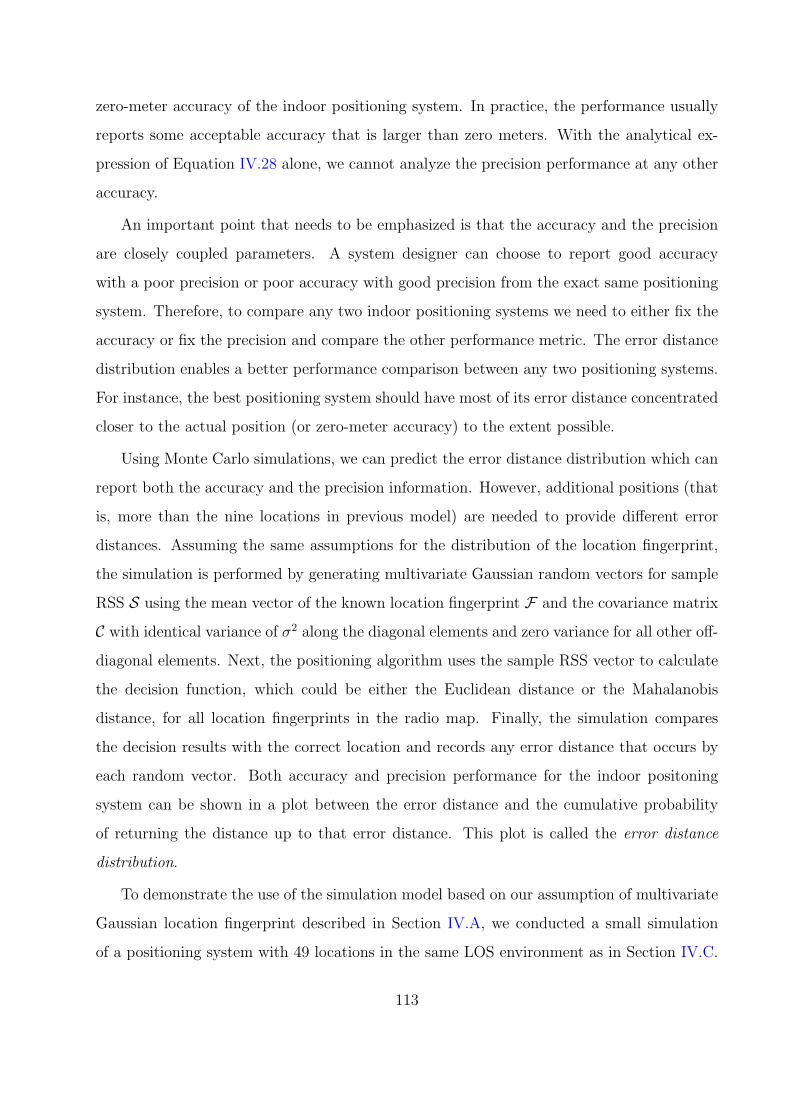
zero-meter accuracy of the indoor positioning system. In practice, the performance usually
reports some acceptable accuracy that is larger than zero meters. With the analytical ex-
pression of Equation IV.28 alone, we cannot analyze the precision performance at any other
accuracy.
An important point that needs to be emphasized is that the accuracy and the precision
are closely coupled parameters. A system designer can choose to report good accuracy
with a poor precision or poor accuracy with good precision from the exact same positioning
system. Therefore, to compare any two indoor positioning systems we need to either fix the
accuracy or fix the precision and compare the other performance metric. The error distance
distribution enables a better performance comparison between any two positioning systems.
For instance, the best positioning system should have most of its error distance concentrated
closer to the actual position (or zero-meter accuracy) to the extent possible.
Using Monte Carlo simulations, we can predict the error distance distribution which can
report both the accuracy and the precision information. However, additional positions (that
is, more than the nine locations in previous model) are needed to provide different error
distances. Assuming the same assumptions for the distribution of the location fingerprint,
the simulation is performed by generating multivariate Gaussian random vectors for sample
RSS S using the mean vector of the known location fingerprint F and the covariance matrix
C with identical variance of σ2 along the diagonal elements and zero variance for all other off-
diagonal elements. Next, the positioning algorithm uses the sample RSS vector to calculate
the decision function, which could be either the Euclidean distance or the Mahalanobis
distance, for all location fingerprints in the radio map. Finally, the simulation compares
the decision results with the correct location and records any error distance that occurs by
each random vector. Both accuracy and precision performance for the indoor positoning
system can be shown in a plot between the error distance and the cumulative probability
of returning the distance up to that error distance. This plot is called the error distance
distribution.
To demonstrate the use of the simulation model based on our assumption of multivariate
Gaussian location fingerprint described in Section IV.A, we conducted a small simulation
of a positioning system with 49 locations in the same LOS environment as in Section IV.C.
113
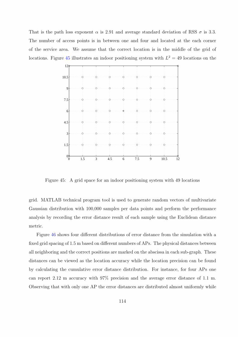
That is the path loss exponent α is 2.91 and average standard deviation of RSS σ is 3.3.
The number of access points is in between one and four and located at the each corner
of the service area. We assume that the correct location is in the middle of the grid of
locations. Figure 45 illustrates an indoor positioning system with L2 = 49 locations on the
0 1.5 3 4.5 6 7.5 9 10.5 120
1.5
3
4.5
6
7.5
9
10.5
12
Figure 45: A grid space for an indoor positioning system with 49 locations
grid. MATLAB technical program tool is used to generate random vectors of multivariate
Gaussian distribution with 100,000 samples per data points and perform the performance
analysis by recording the error distance result of each sample using the Euclidean distance
metric.
Figure 46 shows four different distributions of error distance from the simulation with a
fixed grid spacing of 1.5 m based on different numbers of APs. The physical distances between
all neighboring and the correct positions are marked on the abscissa in each sub-graph. These
distances can be viewed as the location accuracy while the location precision can be found
by calculating the cumulative error distance distribution. For instance, for four APs one
can report 2.12 m accuracy with 97% precision and the average error distance of 1.1 m.
Observing that with only one AP the error distances are distributed almost uniformly while
114
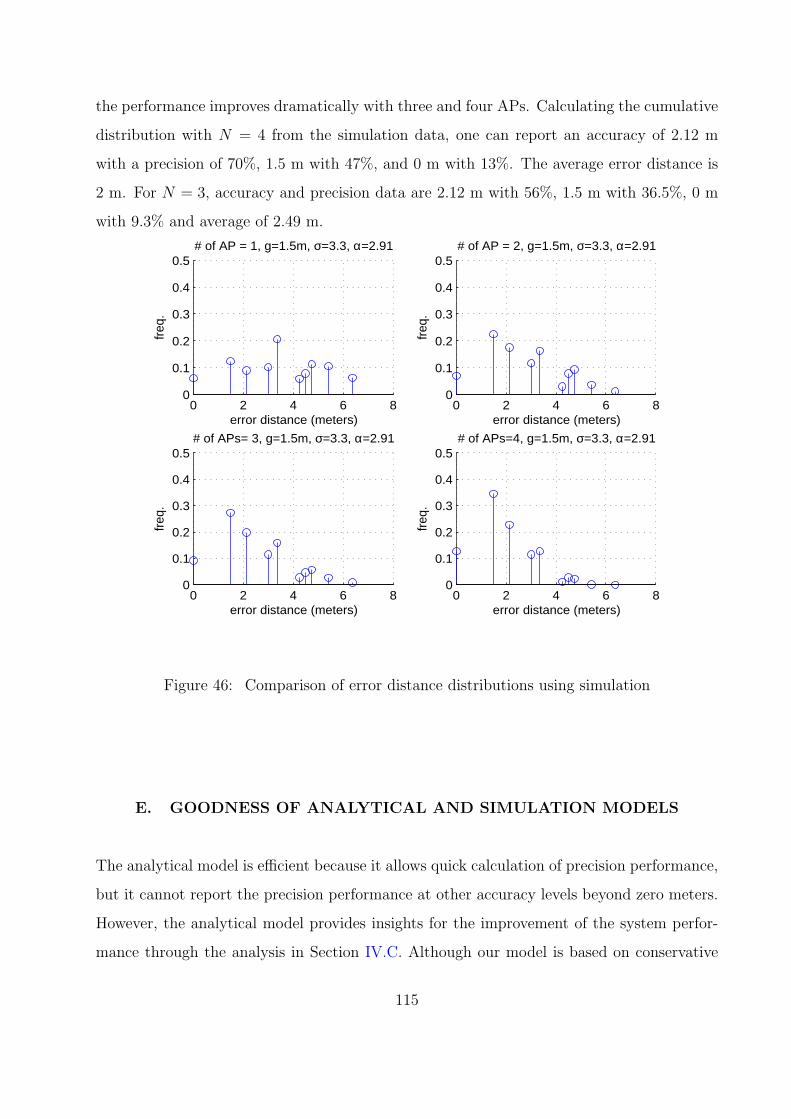
the performance improves dramatically with three and four APs. Calculating the cumulative
distribution with N = 4 from the simulation data, one can report an accuracy of 2.12 m
with a precision of 70%, 1.5 m with 47%, and 0 m with 13%. The average error distance is
2 m. For N = 3, accuracy and precision data are 2.12 m with 56%, 1.5 m with 36.5%, 0 m
with 9.3% and average of 2.49 m.
0 2 4 6 80
0.1
0.2
0.3
0.4
0.5
error distance (meters)
freq
.
# of AP = 1, g=1.5m, σ=3.3, α=2.91
0 2 4 6 80
0.1
0.2
0.3
0.4
0.5
error distance (meters)fr
eq.
# of AP = 2, g=1.5m, σ=3.3, α=2.91
0 2 4 6 80
0.1
0.2
0.3
0.4
0.5
error distance (meters)
freq
.
# of APs= 3, g=1.5m, σ=3.3, α=2.91
0 2 4 6 80
0.1
0.2
0.3
0.4
0.5
error distance (meters)
freq
.# of APs=4, g=1.5m, σ=3.3, α=2.91
Figure 46: Comparison of error distance distributions using simulation
E. GOODNESS OF ANALYTICAL AND SIMULATION MODELS
The analytical model is efficient because it allows quick calculation of precision performance,
but it cannot report the precision performance at other accuracy levels beyond zero meters.
However, the analytical model provides insights for the improvement of the system perfor-
mance through the analysis in Section IV.C. Although our model is based on conservative
115
assumptions, it provides a framework for further creating more complex mathematical mod-
els and representations of indoor positioning system. For instance, we could use different
values for the standard deviation of the RSS value from each access point.
The simulation model is another tool which provides more insights on the distribution of
the error distance. It enables a system designer to approximate both precision and accuracy
performance other than the precision at zero-meter. One advantage of the simulation model
is that it can incorporate non-standardized distributions to model location fingerprint for
analysis of indoor positioning performance. We will demonstrate this point in the next
Chapter. However, the disadvantage of the simulation model is that it may require more
time than the analytical approach. In both cases, our models require a good approximation of
the actual environment parameters such as the path loss exponent, the standard deviation
of the RSS in that environment, and a good prediction of the location fingerprints. The
goodness of our system analysis will depend greatly on the system parameters and the
location fingerprint prediction.
In comparing our mathematical model to a real system, we can identify three major
differences based on the infrastructure, the survey, and the real position. The following
subsections discuss these difference and argues the goodness of our models.
1. Missing Signals
First, in real systems, the access points are installed opportunistically and a MS may not
receive signals from all access points in the building. A subset of access points may be present
in the MS’s view at a particular time. Our measurements in Chapter III indicate that some
APs are never seen for significant durations of time at a location, but suddenly become visible
at other times because of the environmental changes especially in multi-floor environments.
This affects the performance of positioning systems, but we have not incorporated this in
the mathematical model.
This limitation is due to the time dependent property of the RSS, which is difficult to
model. Note that our model assumes a stationary random process. The missing RSS could
occur both during the off-line phase and online phase of the indoor positioning system. To
116
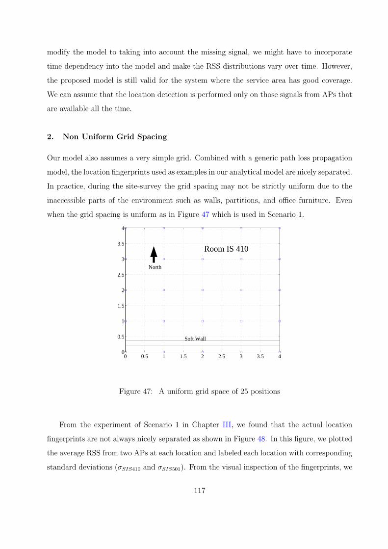
modify the model to taking into account the missing signal, we might have to incorporate
time dependency into the model and make the RSS distributions vary over time. However,
the proposed model is still valid for the system where the service area has good coverage.
We can assume that the location detection is performed only on those signals from APs that
are available all the time.
2. Non Uniform Grid Spacing
Our model also assumes a very simple grid. Combined with a generic path loss propagation
model, the location fingerprints used as examples in our analytical model are nicely separated.
In practice, during the site-survey the grid spacing may not be strictly uniform due to the
inaccessible parts of the environment such as walls, partitions, and office furniture. Even
when the grid spacing is uniform as in Figure 47 which is used in Scenario 1.
0 0.5 1 1.5 2 2.5 3 3.5 40
0.5
1
1.5
2
2.5
3
3.5
4
Soft Wall
North
Room IS 410
Figure 47: A uniform grid space of 25 positions
From the experiment of Scenario 1 in Chapter III, we found that the actual location
fingerprints are not always nicely separated as shown in Figure 48. In this figure, we plotted
the average RSS from two APs at each location and labeled each location with corresponding
standard deviations (σSIS410 and σSIS501). From the visual inspection of the fingerprints, we
117
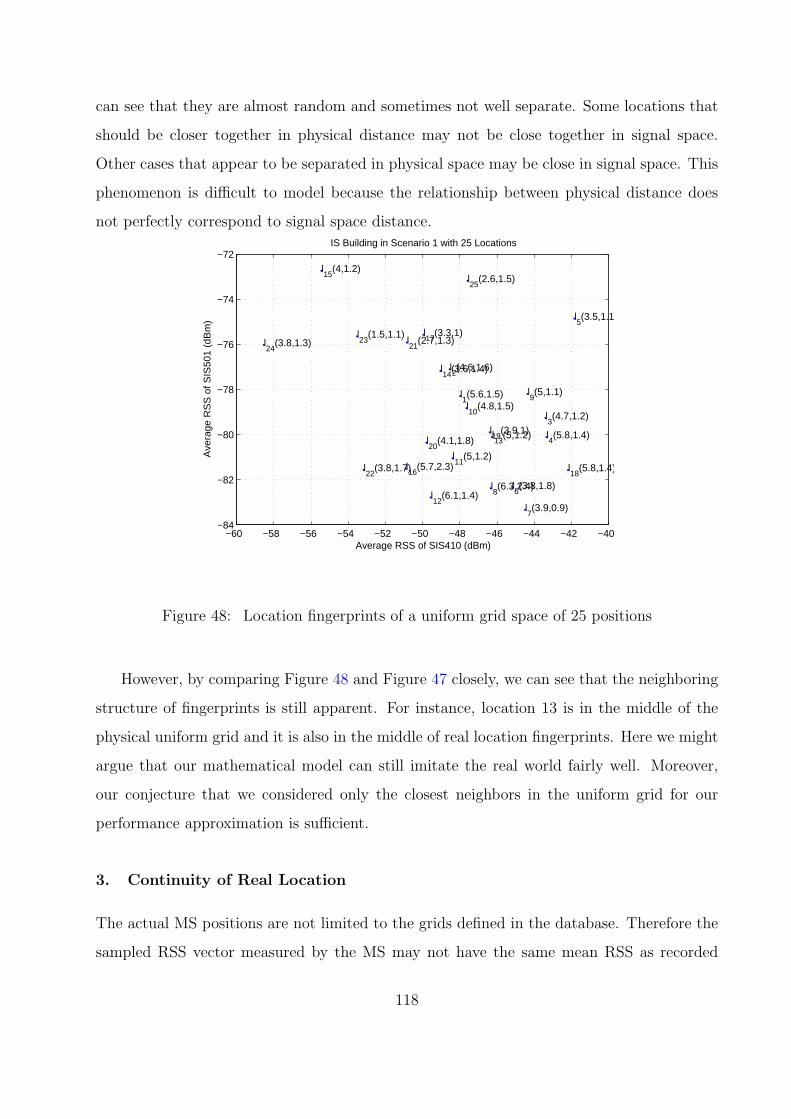
can see that they are almost random and sometimes not well separate. Some locations that
should be closer together in physical distance may not be close together in signal space.
Other cases that appear to be separated in physical space may be close in signal space. This
phenomenon is difficult to model because the relationship between physical distance does
not perfectly correspond to signal space distance.
−60 −58 −56 −54 −52 −50 −48 −46 −44 −42 −40−84
−82
−80
−78
−76
−74
−72
Average RSS of SIS410 (dBm)
Ave
rage
RS
S o
f SIS
501
(dB
m)
IS Building in Scenario 1 with 25 Locations
l1(5.6,1.5)
l2(4.6,1.6)
l3(4.7,1.2)
l4(5.8,1.4)
l5(3.5,1.1)
l6(3.8,1.8)
l7(3.9,0.9)
l8(6.3,2.4)
l9(5,1.1)
l10
(4.8,1.5)
l11
(5,1.2)
l12
(6.1,1.4)
l13
(5,1.2)
l14
(3.6,1.4)
l15
(4,1.2)
l16
(5.7,2.3)
l17
(3.3,1)
l18
(5.8,1.4)
l19
(3.9,1)l20
(4.1,1.8)
l21
(2.7,1.3)
l22
(3.8,1.7)
l23
(1.5,1.1)l24
(3.8,1.3)
l25
(2.6,1.5)
Figure 48: Location fingerprints of a uniform grid space of 25 positions
However, by comparing Figure 48 and Figure 47 closely, we can see that the neighboring
structure of fingerprints is still apparent. For instance, location 13 is in the middle of the
physical uniform grid and it is also in the middle of real location fingerprints. Here we might
argue that our mathematical model can still imitate the real world fairly well. Moreover,
our conjecture that we considered only the closest neighbors in the uniform grid for our
performance approximation is sufficient.
3. Continuity of Real Location
The actual MS positions are not limited to the grids defined in the database. Therefore the
sampled RSS vector measured by the MS may not have the same mean RSS as recorded
118
in the database. This is actually not the problem specific only to the analytical model.
The real indoor positioning system also does not record continuous positions. A real system
also reports the closest location on the grid that the mobile device is at. To imitate the
real system, we could change the model to allow the sample RSS vectors to be generated
based on the mean of locations that are not on the predefined grid. Then, we could simulate
the system to find the error distance distribution. It can be expected that some of the
error distances could be cut into half of the grid spacing because the error distance now
corresponds to a location in the middle of two calibrated locations. However, the precision
reported at zero-meter error distance will be less or none. We believe this is not a significant
limitation of the model since the random variation of the RSS implies that any position
not on a calibrated grid point will likely have a fingerprint that is very close to or almost
identical to those of one of the neighboring grid points.
F. CONCLUSIONS
By looking at the system from the distance comparison approach, this chapter provides a
framework for theoretical explanation and insights about the indoor positioning system.
Equivalent analysis could be done based on the probabilistic approach. Similar results
could be obtained from both approaches because of our simplified mathematical structure
(Gaussian assumption). Given a set of system parameters and radio propagation charac-
teristics, which are the number of access points, the grid spacing, the path loss exponent,
and standard deviation of RSS, the accuracy of the positioning system can be determined
in terms of the probability of returning the correct location with the model presented in
this chapter. The analysis results could lead to a guideline on the parameters to consider in
designing and deploying an indoor positioning system. Monte Carlo simulation of location
fingerprints can be used to create error distance distributions which form a valuable tool to
compare different indoor positioning systems. We will explore the design and deployment of
indoor positioning in the next chapter using the knowledge gained from previous and current
chapters.
119

V. SYSTEM DESIGN AND DEPLOYMENT
While prototypes and commercialized products of WLAN based indoor positioning systems
have been available for quite some time, each system has its own design choice with little
benchmarking and no research focusing on system performance, design and deployment
issues. The study in this chapter discusses design trade-off and performance improvement
conditions. First, Section V.A points out a number of high level design and deployment’s
choices which we derive from experience in the literature and our own measurement analysis
results. Second, Section V.B discusses low level design issues which include the selection of
positioning algorithms and the performance of positioning system. Utilizing our proposed
model, we demonstrate the use of our model to justify the performance improvement which
in turn could provide guideline to improve real system. Third, we summarize a set of design
guidelines in Section V.D which consists of a design checklist and performance improvement
recommendations. Finally, we present our own software-based indoor positioning prototype
based on the Euclidean distance algorithm in Section V.C. We use this prototype to consider
our design decision and validate our model presented in previous chapters.
A. HIGH LEVEL SYSTEM DESIGN
This section identifies a set of design decisions which are relevant to location fingerprinting
types of systems. The top level issues that a designer should consider are application, com-
plexity, performance, and security. These issues will dictate where a system component (such
as sensing point and positioning algorithm) should be placed within the indoor positioning
systems. The result of the discussion in this section is a design checklist which is shown in
120
Section V.D.
1. System Design Issues
The following list briefly describes the design considerations for indoor positioning system.
A system designer must decide or determine these issues before implementing and deploying
the actual positioning system.
Type of Applications is the first design decision that must be determined. The location
fingerprinting technique is generally aimed to provide locating and tracking services to
users inside buildings [13]. Thus far, the best accuracy performance result of such systems
(summarized in Table 4) is still on the order of a few meters of actual location. Due
to the randomness of the RSS as discussed in Chapter III, the WLAN based indoor
positioning systems will not be able to provide centimeter-level accuracy. Therefore,
this kind of positioning system is suitable for the applications that require one or more
meters of accuracy. Fortunately, there are a number of emerging location-based services
for this level of accuracy for indoor environment such as location determination for home
automation [68].
Size of service area influences how many locations are needed to be calibrated. The area
size affects the time required to collect the location fingerprint, and how many access
points are necessary to cover the service area. We also have to make sure that every
location in the service area has sufficient number of different AP’s signals for positioning
purposes.
Location resolution and grid spacing can be determined based on the type of services
the positioning system will provide. Some applications are sufficiently served with an
accuracy commensurate with the size of an office room size (i.e. 5 m.), while other
applications require an order of a couple meters of location granularity (i.e. cubicle size
of 3 m × 3m). Collecting too dense location fingerprints can lead to wasting of time and
effort without gaining improvement in performance. The decision on these parameters
can dictate how scalable the fingerprinting system will be for that particular choice of
grid spacing. We can use the proposed model in Chapter IV to determine suitable grid
121
spacing to meet any required performance goal.
Number of locations depends greatly on the size of service area, the grid spacing and the
actual floor plan. Furniture and inaccessible areas will reduce the number of locations
to perform the fingerprint collection. To decide on number of locations, the help of floor
plan and the results of previous two decisions are required.
Number of access points is the key to improving the performance as we pointed out
in our mathematical description in Chapter IV. Our proposed model in Chapter IV can
help a system designer to estimate the number of access point that could achieve required
performance goal. For indoor positioning purposes, we just need the beacon signal from
the access points for location detection. The access point does not require to be fully
connected to the internet [21]. Fortunately, the price of IEEE 802.11b access points has
been coming down to less than a hundred dollars. Increasing the number of APs does not
cost very much. Although the number of non-overlapping frequencies of IEEE 802.11b
is limited, we can place them close together without much worry about the interference
if data communications is not the main service. Moving access points around to improve
the signal in the area can be easily accomplished as well.
Number of users is another issue that must be considered because it can contributes signif-
icant traffic and work load on the WLAN network infrastructure and positioning server.
For example, if the number of users is large, the location sensing function should be on
the mobile devices rather than on the access points.
User’s Orientation Consideration should be included in the radio map; however, prac-
tical implementation and feasibility of the deployment may force the system designer to
avoid the inclusion of orientation. An example commercial software [21] instructs the user
to turn around 360 degree at each location during the collection of location fingerprints
which takes around 20 seconds. This shows an example of averaging out the fingerprint
across all orientations. If the orientation is decided to be included, the designer must also
decide how many orientations should be included. The more the number of orientations
the larger the number of data must be collected for all combinations of locations and
orientations.
Environment parameters such as the path loss exponent and standard deviation of RSS
122
should be determined by conducting a small site survey. They are required if we want
to predict the performance of positioning system without laborious measurements.
Number of samples for location fingerprinting influences the performance of the sys-
tem. We discussed this number in Chapter III. This number should be determined and
tuned to achieve the required performance goal. Our model did not include this issue
and assume that the statistics in any given location fingerprint from the path loss model
is sufficient.
Fingerprint collection is the most time consuming procedure in WLAN based indoor
positioning system. Without assistance of any signal propagation model to create the
location fingerprint, the measurement period and the number of required samples should
be selected such that the system can be efficiently deployed over large areas. There is a
tradeoff between the performance and the time required to collect the fingerprints. The
shortest data collection period per location should be used to scale the deployment of
such systems as the number of points required to collected is multiplied per area.
Number of samples for detecting location: As pointed out by [13], the average value
of multiple samples could improve the performance of location detection slightly. They
indicated that 3 samples provided almost as good as 20 samples in their experiment.
However, in our model and prototype above we use only one sample to detect the location.
Location sensing side can be determined by the application, required security and pri-
vacy, and the complexity limitation. Both mobile devices (client-side) and access points
(network-side) can transmit beacon signals and perform RSS measurement. Note that
The accuracy performance seems not to be significantly affected by the decision of where
to put the location sensing due to very little asymmetry of signal strength measurement
in [13]. This little impact on accuracy performance is true if the hardware comes from
the same vendor on both the client-side and network-side. For user locating and tracking
applications, it is a logical decision to have a WLAN network perform location sensing.
If the number of users for particular application becomes larger, the location sensing
function should be distributed to the mobile devices to reduce the load and complexity
on a positioning server and access points in network. If the location-based service is in
the form of a resource locator, all the location sensing can be done at the client-side. The
123
client-side RSS measurement can provide more security and privacy for the user. The
system will be more complex for the network-side measurement because the system will
require the cooperation and synchronization of all mobile devices and access points [13].
Positioning calculation side is the issue that may limited by the computing power and
energy of the mobile device. For applications of home and small office with small number
of mobile devices or user locating and tracking applications, the positioning calculation
is more suitable to be done at a centralized server [68]. In some application like resource
locator, location calculation can be done on the mobile devices with necessary information
pre-loaded on the mobile device themselves.
B. LOW LEVEL SYSTEM DESIGN
1. Algorithm Selection
Comparison of WLAN based positioning algorithms was presented in [22], but little dis-
cussion was made regarding their implication on design decisions of the positioning sys-
tem. In [22], the authors estimated the complexity of the off-line phase, the on-line phase
and Vapnik-Chervonenkis dimension1 for weighted k nearest neighbors, probabilistic ap-
proach, neural networks, and statistical learning theory approach or support vector machines
(SVMs). The Vapnik-Chervonenkis dimension is generally used to compare learning algo-
rithms under statistical learning theory. Our scope of study does not include the neural
network and statistical learning theory; therefore, the VC dimension will not be considered
here. This work will only consider design implications of the distance based approach and
probabilistic approach. The Euclidean and the Mahalanobis distance will be analyzed for
the distance based approach, while the probabilistic approach is based on the algorithm used
by [18].
Given an equal set of R training patterns for all algorithms, we estimate the complexity
1Vapnik-Chervonenkis dimension is a measure of any machine learning algorithm on its ability to classifypatterns [42]. It is defined as the maximum number of points that can be arranged so that the machinelearning algorithm can separate them.
124
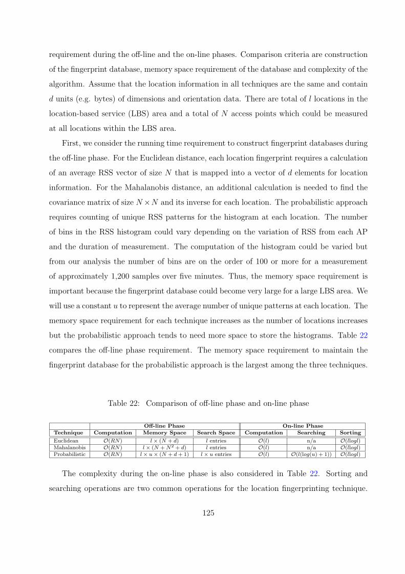
requirement during the off-line and the on-line phases. Comparison criteria are construction
of the fingerprint database, memory space requirement of the database and complexity of the
algorithm. Assume that the location information in all techniques are the same and contain
d units (e.g. bytes) of dimensions and orientation data. There are total of l locations in the
location-based service (LBS) area and a total of N access points which could be measured
at all locations within the LBS area.
First, we consider the running time requirement to construct fingerprint databases during
the off-line phase. For the Euclidean distance, each location fingerprint requires a calculation
of an average RSS vector of size N that is mapped into a vector of d elements for location
information. For the Mahalanobis distance, an additional calculation is needed to find the
covariance matrix of size N×N and its inverse for each location. The probabilistic approach
requires counting of unique RSS patterns for the histogram at each location. The number
of bins in the RSS histogram could vary depending on the variation of RSS from each AP
and the duration of measurement. The computation of the histogram could be varied but
from our analysis the number of bins are on the order of 100 or more for a measurement
of approximately 1,200 samples over five minutes. Thus, the memory space requirement is
important because the fingerprint database could become very large for a large LBS area. We
will use a constant u to represent the average number of unique patterns at each location. The
memory space requirement for each technique increases as the number of locations increases
but the probabilistic approach tends to need more space to store the histograms. Table 22
compares the off-line phase requirement. The memory space requirement to maintain the
fingerprint database for the probabilistic approach is the largest among the three techniques.
Table 22: Comparison of off-line phase and on-line phase
Off-line Phase On-line PhaseTechnique Computation Memory Space Search Space Computation Searching Sorting
Euclidean O(RN) l× (N + d) l entries O(l) n/a O(llogl)Mahalanobis O(RN) l × (N + N2 + d) l entries O(l) n/a O(llogl)Probabilistic O(RN) l× u× (N + d + 1) l× u entries O(l) O(l(log(u) + 1)) O(llogl)
The complexity during the on-line phase is also considered in Table 22. Sorting and
searching operations are two common operations for the location fingerprinting technique.
125
For the Euclidean and the Mahalanobis distances, distance calculations for all locations are
done first. The estimated complexity is shown under the computation column. Then, a
sorting is used to determine the location with the smallest distance. We assume that a
quick sort algorithm is used. For the probabilistic approach, first, the searching (assume
a binary search) for a matching RSS pattern is performed first over the histogram bins in
each location. Next, the posterior probability calculation may be required for all locations.
Finally, a sorting is used to determine the location with the maximum likelihood probability.
The probabilistic approach could require more time to find all matching patterns than the
other two schemes.
Based on the analysis above, the distance based approach requires less memory space to
keep the radio map. The shorter search time of the distance based approach is also another
advantage. However, the probabilistic approach can provide better accuracy and precision
performance because of the extra information in its radio map. Note that in practice the
probabilistic approach require larger number of training samples (R) in order to accurately
approximate the real distribution of location fingerprints; thus, it will take more time to
perform the off-line phase. These issues on design’s tradeoff were not considered previously in
the literature because most of the mobile devices used in the prototypes were powerful laptop
computers. These issues will become important if the radio map and computation are placed
on mobile devices with limited power and computation capabilities. This design decision on
performance tradeoffs should be considered when the computation and the maintaining of
radio map are on the mobile device itself. If a positioning server on the network-side is
dedicated for maintaining the radio map and performing location calculations, the memory
space and computation capability may not be an important design decision.
a. Performance Comparison of Different Positioning Algorithms We analyze
trade-offs of positioning algorithms on the performance by using real location fingerprints
from 25 locations in Scenario 1 of Chapter III. Three APs’ signals (SIS410, SIS401, and
SIS501) were recorded in each fingerprint. We created three different fingerprint databases
or radio maps for the following algorithms: Euclidean distance, Mahalanobis distance, and
probabilistic approach with histogram. The radio map of Euclidean distance contains only
126
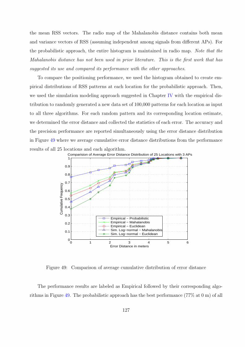
the mean RSS vectors. The radio map of the Mahalanobis distance contains both mean
and variance vectors of RSS (assuming independent among signals from different APs). For
the probabilistic approach, the entire histogram is maintained in radio map. Note that the
Mahalanobis distance has not been used in prior literature. This is the first work that has
suggested its use and compared its performance with the other approaches.
To compare the positioning performance, we used the histogram obtained to create em-
pirical distributions of RSS patterns at each location for the probabilistic approach. Then,
we used the simulation modeling approach suggested in Chapter IV with the empirical dis-
tribution to randomly generated a new data set of 100,000 patterns for each location as input
to all three algorithms. For each random pattern and its corresponding location estimate,
we determined the error distance and collected the statistics of each error. The accuracy and
the precision performance are reported simultaneously using the error distance distribution
in Figure 49 where we average cumulative error distance distributions from the performance
results of all 25 locations and each algorithm.
0 1 2 3 4 5 60
0.1
0.2
0.3
0.4
0.5
0.6
0.7
0.8
0.9
1
Error Distance in meters
Cum
ulat
ive
Freq
uenc
y
Comparision of Average Error Distance Distribution of 25 Locations with 3 APs
Empirical − ProbabilisticEmpirical − MahalanobisEmpirical − EuclideanSim. Log−normal − MahalanobisSim. Log−normal − Euclidean
Figure 49: Comparison of average cumulative distribution of error distance
The performance results are labeled as Empirical followed by their corresponding algo-
rithms in Figure 49. The probabilistic approach has the best performance (77% at 0 m) of all
127
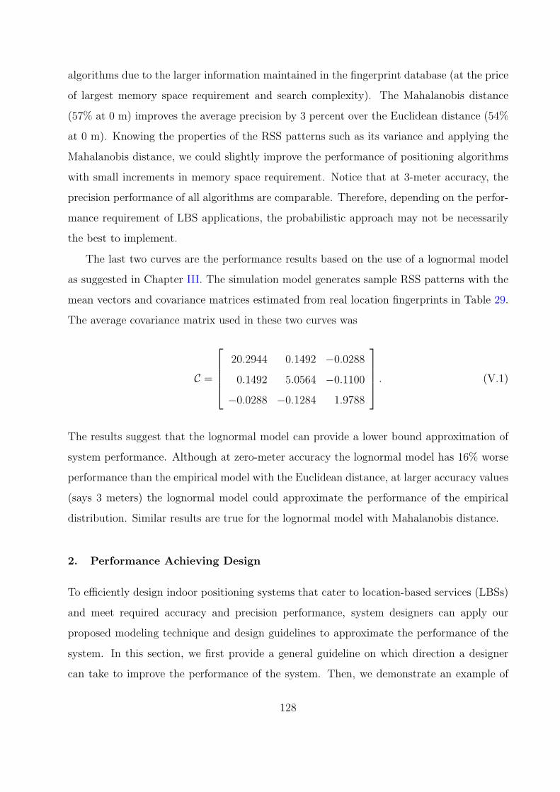
algorithms due to the larger information maintained in the fingerprint database (at the price
of largest memory space requirement and search complexity). The Mahalanobis distance
(57% at 0 m) improves the average precision by 3 percent over the Euclidean distance (54%
at 0 m). Knowing the properties of the RSS patterns such as its variance and applying the
Mahalanobis distance, we could slightly improve the performance of positioning algorithms
with small increments in memory space requirement. Notice that at 3-meter accuracy, the
precision performance of all algorithms are comparable. Therefore, depending on the perfor-
mance requirement of LBS applications, the probabilistic approach may not be necessarily
the best to implement.
The last two curves are the performance results based on the use of a lognormal model
as suggested in Chapter III. The simulation model generates sample RSS patterns with the
mean vectors and covariance matrices estimated from real location fingerprints in Table 29.
The average covariance matrix used in these two curves was
C =
20.2944 0.1492 −0.0288
0.1492 5.0564 −0.1100
−0.0288 −0.1284 1.9788
. (V.1)
The results suggest that the lognormal model can provide a lower bound approximation of
system performance. Although at zero-meter accuracy the lognormal model has 16% worse
performance than the empirical model with the Euclidean distance, at larger accuracy values
(says 3 meters) the lognormal model could approximate the performance of the empirical
distribution. Similar results are true for the lognormal model with Mahalanobis distance.
2. Performance Achieving Design
To efficiently design indoor positioning systems that cater to location-based services (LBSs)
and meet required accuracy and precision performance, system designers can apply our
proposed modeling technique and design guidelines to approximate the performance of the
system. In this section, we first provide a general guideline on which direction a designer
can take to improve the performance of the system. Then, we demonstrate an example of
128
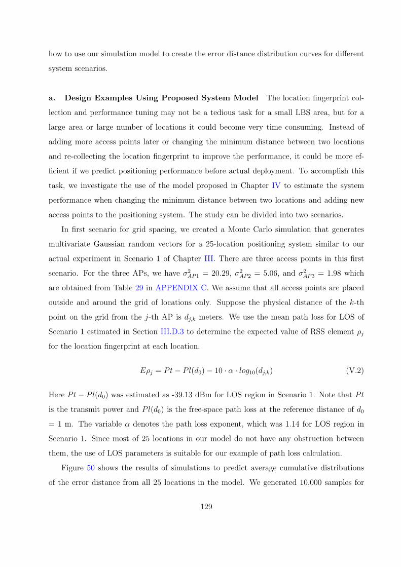
how to use our simulation model to create the error distance distribution curves for different
system scenarios.
a. Design Examples Using Proposed System Model The location fingerprint col-
lection and performance tuning may not be a tedious task for a small LBS area, but for a
large area or large number of locations it could become very time consuming. Instead of
adding more access points later or changing the minimum distance between two locations
and re-collecting the location fingerprint to improve the performance, it could be more ef-
ficient if we predict positioning performance before actual deployment. To accomplish this
task, we investigate the use of the model proposed in Chapter IV to estimate the system
performance when changing the minimum distance between two locations and adding new
access points to the positioning system. The study can be divided into two scenarios.
In first scenario for grid spacing, we created a Monte Carlo simulation that generates
multivariate Gaussian random vectors for a 25-location positioning system similar to our
actual experiment in Scenario 1 of Chapter III. There are three access points in this first
scenario. For the three APs, we have σ2AP1 = 20.29, σ2
AP2 = 5.06, and σ2AP3 = 1.98 which
are obtained from Table 29 in APPENDIX C. We assume that all access points are placed
outside and around the grid of locations only. Suppose the physical distance of the k-th
point on the grid from the j-th AP is dj,k meters. We use the mean path loss for LOS of
Scenario 1 estimated in Section III.D.3 to determine the expected value of RSS element ρj
for the location fingerprint at each location.
Eρj = Pt− Pl(d0)− 10 · α · log10(dj,k) (V.2)
Here Pt− Pl(d0) was estimated as -39.13 dBm for LOS region in Scenario 1. Note that Pt
is the transmit power and Pl(d0) is the free-space path loss at the reference distance of d0
= 1 m. The variable α denotes the path loss exponent, which was 1.14 for LOS region in
Scenario 1. Since most of 25 locations in our model do not have any obstruction between
them, the use of LOS parameters is suitable for our example of path loss calculation.
Figure 50 shows the results of simulations to predict average cumulative distributions
of the error distance from all 25 locations in the model. We generated 10,000 samples for
129
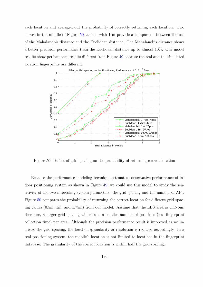
each location and averaged out the probability of correctly returning each location. Two
curves in the middle of Figure 50 labeled with 1 m provide a comparison between the use
of the Mahalanobis distance and the Euclidean distance. The Mahalanobis distance shows
a better precision performance than the Euclidean distance up to almost 10%. Our model
results show performance results different from Figure 49 because the real and the simulated
location fingerprints are different.
0 1 2 3 4 5 60
0.1
0.2
0.3
0.4
0.5
0.6
0.7
0.8
0.9
1
Error Distance in Meters
Cum
ulat
ive
Fre
quen
cy
Effect of Gridspacing on the Positioning Performance of 5x5 m2 Area
Mahalanobis, 1.75m, 4posEuclidean, 1.75m, 4posMahalanobis, 1m, 25posEuclidean, 1m, 25posMahalanobis, 0.5m, 100posEuclidean, 0.5m, 100pos
Figure 50: Effect of grid spacing on the probability of returning correct location
Because the performance modeling technique estimates conservative performance of in-
door positioning system as shown in Figure 49, we could use this model to study the sen-
sitivity of the two interesting system parameters: the grid spacing and the number of APs.
Figure 50 compares the probability of returning the correct location for different grid spac-
ing values (0.5m, 1m, and 1.75m) from our model. Assume that the LBS area is 5m×5m;
therefore, a larger grid spacing will result in smaller number of positions (less fingerprint
collection time) per area. Although the precision performance result is improved as we in-
crease the grid spacing, the location granularity or resolution is reduced accordingly. In a
real positioning system, the mobile’s location is not limited to locations in the fingerprint
database. The granularity of the correct location is within half the grid spacing.
130
As we pointed out earlier, additional access points in the RSS pattern add dimensions
and improve separability among the location fingerprints. There is a diminishing return
on the increment of number of access points [69]. However, this diminishing return also
depends on the number of the locations in the area needed to be identified. A larger number
of locations can affect the number of required APs. Depending on the choice of using existing
access points or installing extra access points for positioning purposes, the location of the
access point could improve the performance of the system. The AP that is far away from
the LBS area and has small signal variation can improve the precision performance better
than the one with larger signal variation.
0 1 2 3 4 5 60
0.1
0.2
0.3
0.4
0.5
0.6
0.7
0.8
0.9
1
Error Distance in meters
Cum
ulat
ive
Fre
quen
cy
Model of 25 locations in area of 5× 5 m2
1 AP with σ2 = 20.29
2 APs with σ2 = 5.06
3 APs with σ2 = 1.98
4 APs with σ2 = 20.29
5 APs with σ2 = 5.06
6 APs with σ2 = 1.98
7 APs with σ2 = 5.06
8 APs with σ2 = 1.98
Figure 51: Effect of number of access point on the error distance distribution
Figure 51 illustrates the performance improvement to the model of 25 locations when the
number of APs is increased while the grid spacing is fixed at 1 m. In this second scenario of
increasing number of access points, we used the same number of samples as the first scenario
in Figure 50 (10,000 samples) per location and average out the the probability of correctly
returning each location. In this scenario, we assume that the 4th to 6th APs have the same
variance as the 1st to 3rd APs which are 20.29, 5.06, and 1.98, respectively. The 7th and
the 8th APs have the same covariance matrix as the 2nd and the 3rd APs which is 5.06 and
131
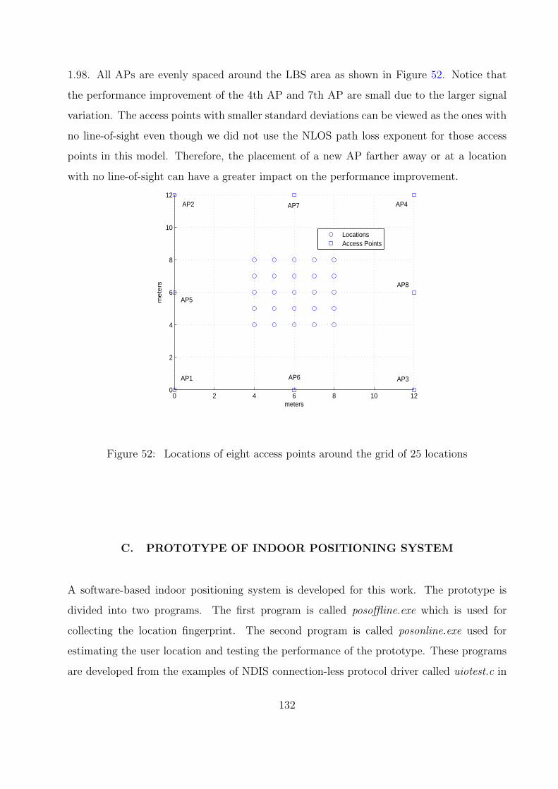
1.98. All APs are evenly spaced around the LBS area as shown in Figure 52. Notice that
the performance improvement of the 4th AP and 7th AP are small due to the larger signal
variation. The access points with smaller standard deviations can be viewed as the ones with
no line-of-sight even though we did not use the NLOS path loss exponent for those access
points in this model. Therefore, the placement of a new AP farther away or at a location
with no line-of-sight can have a greater impact on the performance improvement.
0 2 4 6 8 10 120
2
4
6
8
10
12
meters
me
ters
LocationsAccess Points
AP1
AP8
AP6
AP5
AP3
AP2 AP7 AP4
Figure 52: Locations of eight access points around the grid of 25 locations
C. PROTOTYPE OF INDOOR POSITIONING SYSTEM
A software-based indoor positioning system is developed for this work. The prototype is
divided into two programs. The first program is called posoffline.exe which is used for
collecting the location fingerprint. The second program is called posonline.exe used for
estimating the user location and testing the performance of the prototype. These programs
are developed from the examples of NDIS connection-less protocol driver called uiotest.c in
132
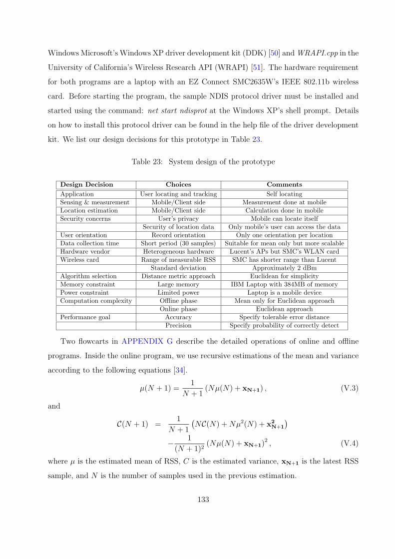
Windows Microsoft’s Windows XP driver development kit (DDK) [50] and WRAPI.cpp in the
University of California’s Wireless Research API (WRAPI) [51]. The hardware requirement
for both programs are a laptop with an EZ Connect SMC2635W’s IEEE 802.11b wireless
card. Before starting the program, the sample NDIS protocol driver must be installed and
started using the command: net start ndisprot at the Windows XP’s shell prompt. Details
on how to install this protocol driver can be found in the help file of the driver development
kit. We list our design decisions for this prototype in Table 23.
Table 23: System design of the prototype
Design Decision Choices CommentsApplication User locating and tracking Self locatingSensing & measurement Mobile/Client side Measurement done at mobileLocation estimation Mobile/Client side Calculation done in mobileSecurity concerns User’s privacy Mobile can locate itself
Security of location data Only mobile’s user can access the dataUser orientation Record orientation Only one orientation per locationData collection time Short period (30 samples) Suitable for mean only but more scalableHardware vendor Heterogeneous hardware Lucent’s APs but SMC’s WLAN cardWireless card Range of measurable RSS SMC has shorter range than Lucent
Standard deviation Approximately 2 dBmAlgorithm selection Distance metric approach Euclidean for simplicityMemory constraint Large memory IBM Laptop with 384MB of memoryPower constraint Limited power Laptop is a mobile deviceComputation complexity Offline phase Mean only for Euclidean approach
Online phase Euclidean approachPerformance goal Accuracy Specify tolerable error distance
Precision Specify probability of correctly detect
Two flowcarts in APPENDIX G describe the detailed operations of online and offline
programs. Inside the online program, we use recursive estimations of the mean and variance
according to the following equations [34].
µ(N + 1) =1
N + 1(Nµ(N) + xN+1) , (V.3)
and
C(N + 1) =1
N + 1
(NC(N) + Nµ2(N) + x2
N+1
)
− 1
(N + 1)2(Nµ(N) + xN+1)
2 , (V.4)
where µ is the estimated mean of RSS, C is the estimated variance, xN+1 is the latest RSS
sample, and N is the number of samples used in the previous estimation.
133
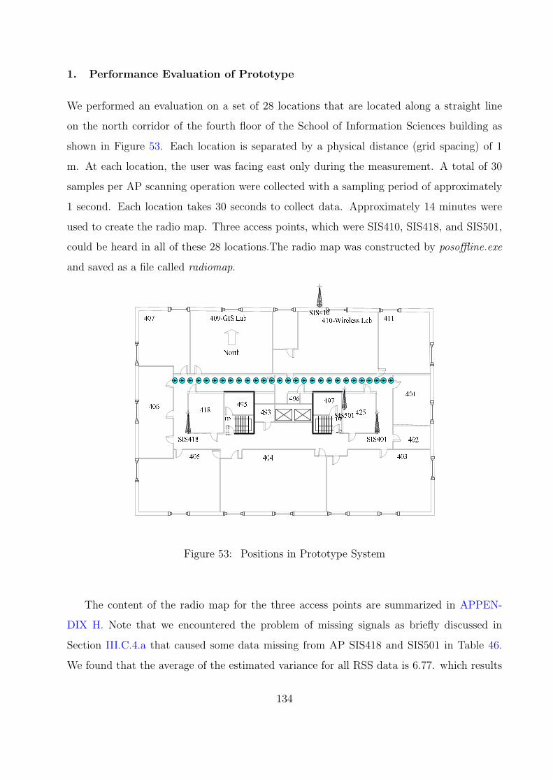
1. Performance Evaluation of Prototype
We performed an evaluation on a set of 28 locations that are located along a straight line
on the north corridor of the fourth floor of the School of Information Sciences building as
shown in Figure 53. Each location is separated by a physical distance (grid spacing) of 1
m. At each location, the user was facing east only during the measurement. A total of 30
samples per AP scanning operation were collected with a sampling period of approximately
1 second. Each location takes 30 seconds to collect data. Approximately 14 minutes were
used to create the radio map. Three access points, which were SIS410, SIS418, and SIS501,
could be heard in all of these 28 locations.The radio map was constructed by posoffline.exe
and saved as a file called radiomap.
UPDN UPDN405 404 403402406407
401411
425418 493 496495 497409-GIS Lab 410-Wireless LabSIS410
SIS418 SIS501 SIS401North
Figure 53: Positions in Prototype System
The content of the radio map for the three access points are summarized in APPEN-
DIX H. Note that we encountered the problem of missing signals as briefly discussed in
Section III.C.4.a that caused some data missing from AP SIS418 and SIS501 in Table 46.
We found that the average of the estimated variance for all RSS data is 6.77. which results
134
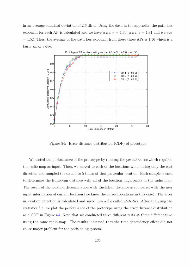
in an average standard deviation of 2.6 dBm. Using the data in the appendix, the path loss
exponent for each AP is calculated and we have αSIS410 = 1.36, αSIS418 = 1.81 and αSIS501
= 1.52. Thus, the average of the path loss exponent from these three APs is 1.56 which is a
fairly small value.
0 5 10 15 20 25 300.2
0.3
0.4
0.5
0.6
0.7
0.8
0.9
1
Error Distance in Meters
Cum
ulat
ive
Den
sity
Fun
ctio
n (C
DF
)
Prototype of 28 locations with gs = 1 m, APs = 3, σ = 2.6, α = 1.56
Test 1 (2 Feb 05)Test 2 (7 Feb 05)Test 3 (7 Feb 05)
Figure 54: Error distance distribution (CDF) of prototype
We tested the performance of the prototype by running the posonline.exe which required
the radio map as input. Then, we moved to each of the locations while facing only the east
direction and sampled the data 4 to 5 times at that particular location. Each sample is used
to determine the Euclidean distance with all of the location fingerprints in the radio map.
The result of the location determination with Euclidean distance is compared with the user
input information of current location (we knew the correct locations in this case). The error
in location detection is calculated and saved into a file called statistics. After analyzing the
statistics file, we plot the performance of the prototype using the error distance distribution
as a CDF in Figure 54. Note that we conducted three different tests at three different time
using the same radio map. The results indicated that the time dependency effect did not
cause major problem for the positioning system.
135
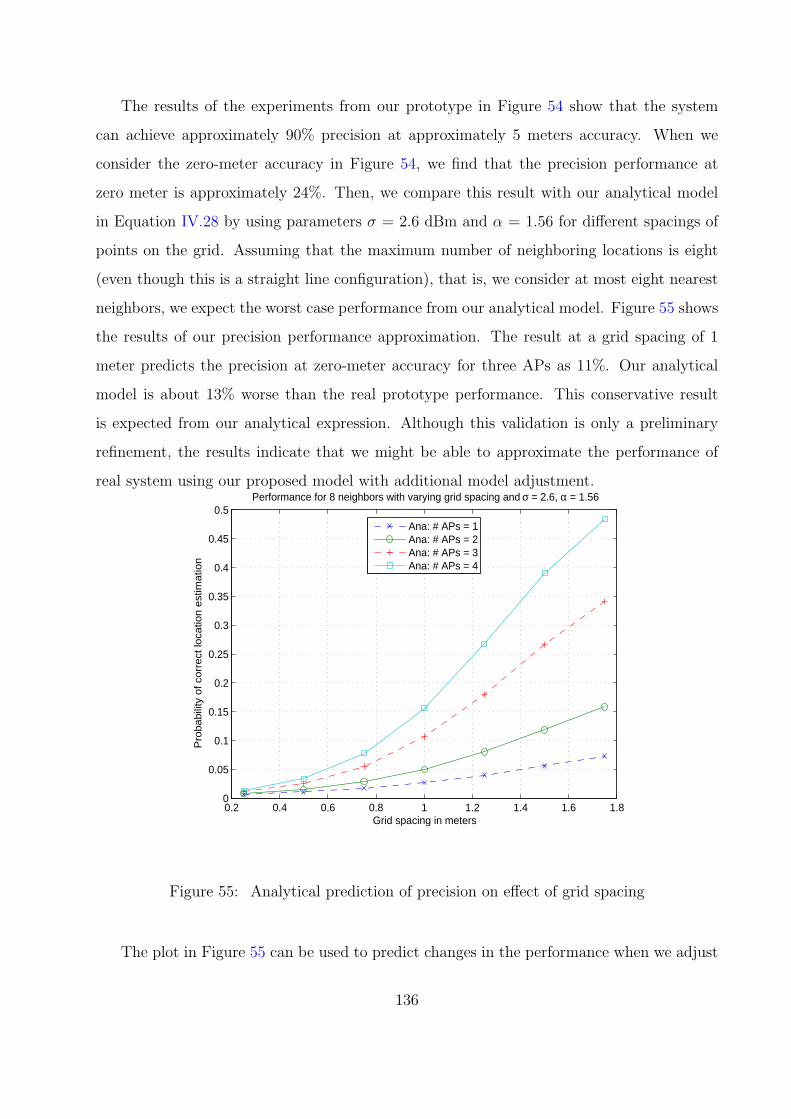
The results of the experiments from our prototype in Figure 54 show that the system
can achieve approximately 90% precision at approximately 5 meters accuracy. When we
consider the zero-meter accuracy in Figure 54, we find that the precision performance at
zero meter is approximately 24%. Then, we compare this result with our analytical model
in Equation IV.28 by using parameters σ = 2.6 dBm and α = 1.56 for different spacings of
points on the grid. Assuming that the maximum number of neighboring locations is eight
(even though this is a straight line configuration), that is, we consider at most eight nearest
neighbors, we expect the worst case performance from our analytical model. Figure 55 shows
the results of our precision performance approximation. The result at a grid spacing of 1
meter predicts the precision at zero-meter accuracy for three APs as 11%. Our analytical
model is about 13% worse than the real prototype performance. This conservative result
is expected from our analytical expression. Although this validation is only a preliminary
refinement, the results indicate that we might be able to approximate the performance of
real system using our proposed model with additional model adjustment.
0.2 0.4 0.6 0.8 1 1.2 1.4 1.6 1.80
0.05
0.1
0.15
0.2
0.25
0.3
0.35
0.4
0.45
0.5
Grid spacing in meters
Pro
babi
lity
of c
orre
ct lo
catio
n es
timat
ion
Performance for 8 neighbors with varying grid spacing and σ = 2.6, α = 1.56
Ana: # APs = 1Ana: # APs = 2Ana: # APs = 3Ana: # APs = 4
Figure 55: Analytical prediction of precision on effect of grid spacing
The plot in Figure 55 can be used to predict changes in the performance when we adjust
136
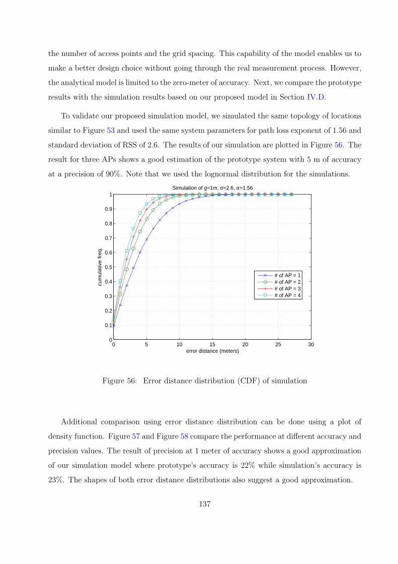
the number of access points and the grid spacing. This capability of the model enables us to
make a better design choice without going through the real measurement process. However,
the analytical model is limited to the zero-meter of accuracy. Next, we compare the prototype
results with the simulation results based on our proposed model in Section IV.D.
To validate our proposed simulation model, we simulated the same topology of locations
similar to Figure 53 and used the same system parameters for path loss exponent of 1.56 and
standard deviation of RSS of 2.6. The results of our simulation are plotted in Figure 56. The
result for three APs shows a good estimation of the prototype system with 5 m of accuracy
at a precision of 90%. Note that we used the lognormal distribution for the simulations.
0 5 10 15 20 25 300
0.1
0.2
0.3
0.4
0.5
0.6
0.7
0.8
0.9
1
error distance (meters)
cum
ulat
ive
freq
.
Simulation of g=1m, σ=2.6, α=1.56
# of AP = 1# of AP = 2# of AP = 3# of AP = 4
Figure 56: Error distance distribution (CDF) of simulation
Additional comparison using error distance distribution can be done using a plot of
density function. Figure 57 and Figure 58 compare the performance at different accuracy and
precision values. The result of precision at 1 meter of accuracy shows a good approximation
of our simulation model where prototype’s accuracy is 22% while simulation’s accuracy is
23%. The shapes of both error distance distributions also suggest a good approximation.
137
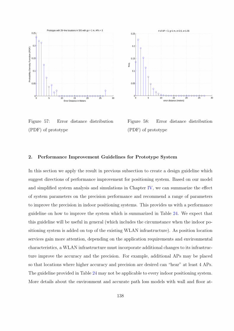
0 5 10 15 20 25 300
0.05
0.1
0.15
0.2
0.25
Error Distance in Meters
Pro
ba
bili
ty D
en
sity
Fu
nct
ion
(P
DF
)Prototype with 28−line locations in SIS with gs = 1 m, APs = 3
Figure 57: Error distance distribution
(PDF) of prototype
0 5 10 15 20 25 300
0.05
0.1
0.15
0.2
0.25
error distance (meters)
fre
q.
# of AP = 3, g=1 m, σ=2.6, α=1.56
Figure 58: Error distance distribution
(PDF) of prototype
2. Performance Improvement Guidelines for Prototype System
In this section we apply the result in previous subsection to create a design guideline which
suggest directions of performance improvement for positioning system. Based on our model
and simplified system analysis and simulations in Chapter IV, we can summarize the effect
of system parameters on the precision performance and recommend a range of parameters
to improve the precision in indoor positioning systems. This provides us with a performance
guideline on how to improve the system which is summarized in Table 24. We expect that
this guideline will be useful in general (which includes the circumstance when the indoor po-
sitioning system is added on top of the existing WLAN infrastructure). As position location
services gain more attention, depending on the application requirements and environmental
characteristics, a WLAN infrastructure must incorporate additional changes to its infrastruc-
ture improve the accuracy and the precision. For example, additional APs may be placed
so that locations where higher accuracy and precision are desired can “hear” at least 4 APs.
The guideline provided in Table 24 may not be applicable to every indoor positioning system.
More details about the environment and accurate path loss models with wall and floor at-
138

tenuation could result in a more realistic recommendation for the deployment process using
our framework proposed here.
Table 24: Recommended values for location system parameters
Parameters Value Increased Desired Rangeσ - STD. of Gaussian component precision decreases & accuracy decrease σ < 3
N - Number of access points precision increases & accuracy increase N ≥ 4α - Path loss exponent precision increases & accuracy increase α > 3.5
(better in NLOS area)g - grid spacing precision increases & accuracy decrease g > 1.25 meter
D. HIGH LEVEL DESIGN GUIDELINES
1. Design Decision Guidelines
Table 25 summarizes all design decisions in SectionV.A. The table provides brief comments
on each design choice which can help decide during the high level design phase. We demon-
strated the use this design guideline to assist the development of the prototype of software-
based indoor positioning system in the previous section. This table serves as a first step of
our set of design guidelines.
E. CONCLUSIONS
This chapter is the most crucial contribution for the indoor positioning system because the
currently deployment of indoor positioning based on location fingerprinting is expected to
be very time-consuming for the off-line phase. That is the system designer must perform the
data collection first and then test for the positioning performance. If we could predict the
performance of the system without exhaustive real measurement and testing, the deployment
of this system will be much easier and faster. A system design guideline given in this chapter
is the final contribution of this research.
139
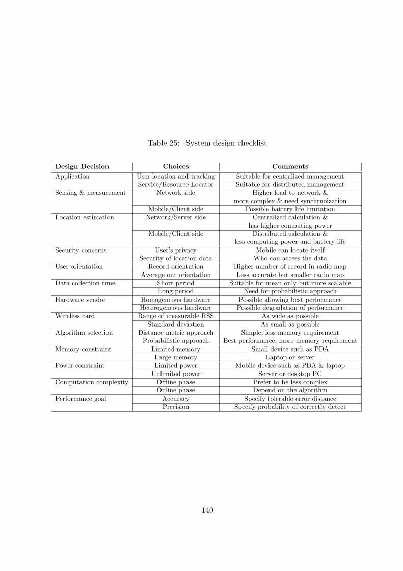
Table 25: System design checklist
Design Decision Choices CommentsApplication User location and tracking Suitable for centralized management
Service/Resource Locator Suitable for distributed managementSensing & measurement Network side Higher load to network &
more complex & need synchrnoizationMobile/Client side Possible battery life limitation
Location estimation Network/Server side Centralized calculation &has higher computing power
Mobile/Client side Distributed calculation &less computing power and battery life
Security concerns User’s privacy Mobile can locate itselfSecurity of location data Who can access the data
User orientation Record orientation Higher number of record in radio mapAverage out orientation Less accurate but smaller radio map
Data collection time Short period Suitable for mean only but more scalableLong period Need for probabilistic approach
Hardware vendor Homogeneous hardware Possible allowing best performanceHeterogeneous hardware Possible degradation of performance
Wireless card Range of measurable RSS As wide as possibleStandard deviation As small as possible
Algorithm selection Distance metric approach Simple, less memory requirementProbabilistic approach Best performance, more memory requirement
Memory constraint Limited memory Small device such as PDALarge memory Laptop or server
Power constraint Limited power Mobile device such as PDA & laptopUnlimited power Server or desktop PC
Computation complexity Offline phase Prefer to be less complexOnline phase Depend on the algorithm
Performance goal Accuracy Specify tolerable error distancePrecision Specify probability of correctly detect
140
VI. CONCLUSIONS AND FUTURE WORK
While empirical results and performance studies of positioning systems based on location
fingerprinting have been presented in the literature, analytical models that can be used
as a framework for efficiently designing the positioning systems are not available. This
dissertation has developed an analytical model as a design tool and recommends a set of
design guidelines for such positioning systems in order to expedite the deployment process.
A system designer can use this framework to strike a balance between the accuracy, the
precision, the location granularity, the number of access points, and the location spacing.
The location fingerprint based on the received signal strength was investigated extensively
in Chapter III. A systematic study was used to analyze the location fingerprint and discover
its unique properties. We found that the RSS is random, with primarily a left-skewed
distribution irrespective of the make of the WLAN card. In some cases, it is possible to
approximate the RSS as being normally distributed. We also found that while the RSS
random process is non-stationary, the mean is more or less constant and could be used
as the fingerprint of a location. Based on exhaustive measurements, we analyzed these and
other properties of the RSS and came up with a mathematically tractable set of assumptions
that enable us to create a model to predict the performance of the system in Chapter III. In
Chapter IV, we used these assumptions to develop a model that can be used with analytical
expressions to determine the probability of correctly estimating the position location of a
mobile device with a single RSS sample vector (precision at zero-meter accuracy). We also
suggested the use of simulation model to predict the distribution of distance error in the
estimate of the position.
We applied the system model proposed in Chapter IV to create a design framework as
discussed in Chapter V. The design framework and guideline suggested in Chapter V provides
141
insights on how to efficiently deploy the indoor positioning system. Accuracy and precision
are the two major performance metrics in this study. Given a set of performance requirements
such as X meters of accuracy and Y % of precision and radio propagation parameters such as
α path loss exponent, the design framework can provide necessary system design guidelines
such as the necessary number of access points and the minimum distance between two closest
positions that can achieve those requirements.
The sensitivity analysis among the system parameters and the performance metrics were
done using the proposed model as showed in Chapter IV. For instance, our study found that
increasing the number of access points could improve the performance of the system, but
there is a diminishing return on the improvement up to certain number of access points. The
effect of radio propagation represented by path loss model suggests that a higher attenuation
in the environment may actually improve the separation of the location fingerprints. The
minimum distance between two adjacent positions also effects the positioning performance.
If two positions are nicely separated, the likelihood that two location fingerprints will be
confused with each other is small. On the other hand, too small a spacing between any
two physical locations will not improve the system performance much. This is due to the
randomness of RSS patterns induced by the ever changing indoor environment. Given the
average standard deviation of the location fingerprints, a designer could identify the minimum
distance separation between two positions that could achieve required performance criteria
as showed in Section V.C.1.
A. CONTRIBUTIONS
This section list the major contribution of this thesis:
I. Extensive measurement analyses of RSS were presented where we confirmed several prop-
erties of the RSS. We used visualization to understand the RSS and its patterns in a
greater detail. We summarized the key properties of the RSS and used it to support
our mathematical model. Although we found that the distribution of RSS has a unique
left-skew property, some distributions could be approximated as lognormal. Because the
142

randomness of the RSS is the cause of difficulty in location determination, we learn that
there are ways to mitigate its effect such as separating the locations apart and increasing
the number of access points.
II. We proposed both analytical and simulation models which are based on assumptions
that are backed by our extensive measurement campaign. We interpreted the underlying
mechanism of indoor positioning system based on location fingerprint using the distance
based approach. We identified major parameters that contribute to the performance of
indoor positioning system based on location fingerprinting.
III. We provided an example of a design guideline which will be useful for approximating the
performance of indoor positioning without doing the real measurement evaluation of the
whole system.
IV. We developed a prototype of indoor positioning system which runs on Windows XP and
is easy to use. It was used to validate our analytical model. We found that our analytical
model could provide sufficient performance approximation to a real system.
B. FUTURE RESEARCH WORK
The research in this thesis provides a ground work for the future study of efficient design
of indoor positioning systems. For instance, we could consider an analytical model that can
approximate the precision performance at any other accuracy performance beyond the zero-
meter accuracy. The non-standard left-skew distribution of RSS could be modeled by the
combination of two different Gaussian distributions to provide a more accurate mathematical
model. The problem of WLAN access point placement which is aimed to provide indoor
positioning system has not been explored in great detail.
The proposed framework still has limitations. First, it did not model the time depen-
dency of the location fingerprints. Thus, the future research study should address this issue.
Second, the indoor positioning system in this study depends greatly on existing infrastructure
of WLAN which has its main purpose for communications. The design guidelines provided
by this study may create a conflict to the design of WLAN. A possible research topic based
143
on the placement of access points to provide both communications and position location ser-
vice should be explored in the future. Third, the relationship between the grid spacing and
the quantization of the wireless cards still requires further investigation. It might be pos-
sible to estimate the number of unique locations in indoor positioning system based on the
knowledge of quantization level of a wireless card and the number of access points. Fourth,
to improve the performance of the system we need to find a solution to deal with those
incomplete or missing data during the off-line and the on-line phases. Fifth, the movement
of user has not been considered in this study. The consideration of location fingerprints of
slow mobility could provide an additional level of understanding of location fingerprinting
systems.
Three more interesting research paths are possible. First, the unified performance evalu-
ation methodology for all indoor positioning system based on location fingerprint is needed
to allow a fair comparison among variety of emerging indoor positioning systems. So far, the
accuracy and the precision are the only performance metrics used for comparison. Second,
a study of the indoor positioning system on with multi-floor and three-dimensional coordi-
nates is not available. The impact of multiple floors is not yet known. Finally, there is a
possible improvement of the location fingerprinting technique with the recent introduction of
multicarrier modulation called orthogonal frequency division multiplexing (OFDM) which is
used by IEEE 802.11a [70] and g [71]. This new modulation technique opens an opportunity
for the location fingerprint to exploit the fingerprint in frequency domain, based on the as-
sumption that frequency selective fading effect might be dependent on the location as well.
However, to the best of our knowledge, there is currently no software device driver that can
collect the received signal levels of multiple carriers from IEEE 802.11a NIC. To prove the
earlier assumption, we could use an electrical network analyzer to measure the dependency
between the frequency selective radio channel and the location. The major benefit from this
new scheme is that location fingerprinting could possibly be done with high accuracy and
precision using only one WLAN access point.
144
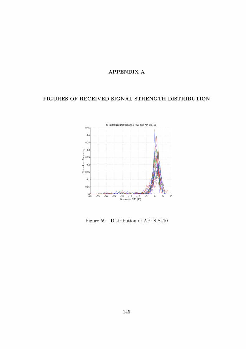
APPENDIX A
FIGURES OF RECEIVED SIGNAL STRENGTH DISTRIBUTION
−40 −35 −30 −25 −20 −15 −10 −5 0 5 100
0.05
0.1
0.15
0.2
0.25
0.3
0.35
0.4
0.45
Normalized RSS (dB)
No
rma
lize
d F
req
ue
ncy
25 Normalized Distributions of RSS from AP: SIS410
Figure 59: Distribution of AP: SIS410
145
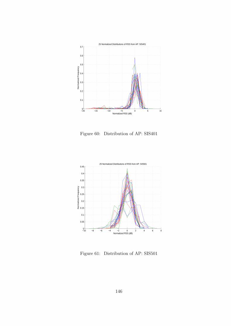
−20 −15 −10 −5 0 5 100
0.1
0.2
0.3
0.4
0.5
0.6
0.7
Normalized RSS (dB)
No
rma
lize
d F
req
ue
ncy
25 Normalized Distributions of RSS from AP: SIS401
Figure 60: Distribution of AP: SIS401
−10 −8 −6 −4 −2 0 2 4 6 80
0.05
0.1
0.15
0.2
0.25
0.3
0.35
0.4
0.45
Normalized RSS (dB)
No
rma
lize
d F
req
ue
ncy
25 Normalized Distributions of RSS from AP: SIS501
Figure 61: Distribution of AP: SIS501
146
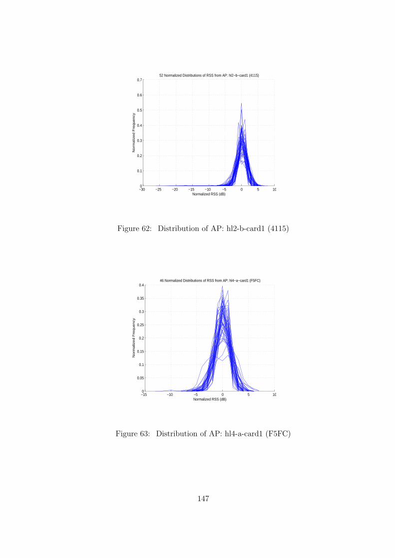
−30 −25 −20 −15 −10 −5 0 5 100
0.1
0.2
0.3
0.4
0.5
0.6
0.7
Normalized RSS (dB)
No
rma
lize
d F
req
ue
ncy
52 Normalized Distributions of RSS from AP: hl2−b−card1 (4115)
Figure 62: Distribution of AP: hl2-b-card1 (4115)
−15 −10 −5 0 5 100
0.05
0.1
0.15
0.2
0.25
0.3
0.35
0.4
Normalized RSS (dB)
No
rma
lize
d F
req
ue
ncy
46 Normalized Distributions of RSS from AP: hl4−a−card1 (F5FC)
Figure 63: Distribution of AP: hl4-a-card1 (F5FC)
147
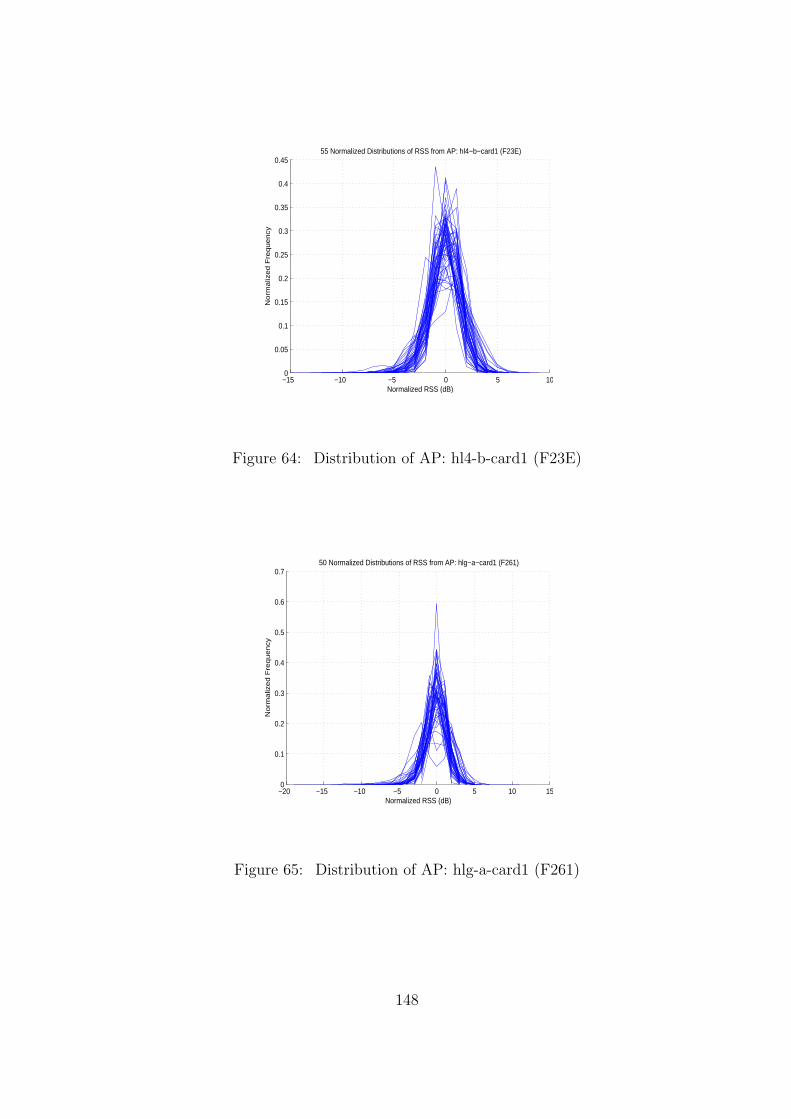
−15 −10 −5 0 5 100
0.05
0.1
0.15
0.2
0.25
0.3
0.35
0.4
0.45
Normalized RSS (dB)
No
rma
lize
d F
req
ue
ncy
55 Normalized Distributions of RSS from AP: hl4−b−card1 (F23E)
Figure 64: Distribution of AP: hl4-b-card1 (F23E)
−20 −15 −10 −5 0 5 10 150
0.1
0.2
0.3
0.4
0.5
0.6
0.7
Normalized RSS (dB)
No
rma
lize
d F
req
ue
ncy
50 Normalized Distributions of RSS from AP: hlg−a−card1 (F261)
Figure 65: Distribution of AP: hlg-a-card1 (F261)
148
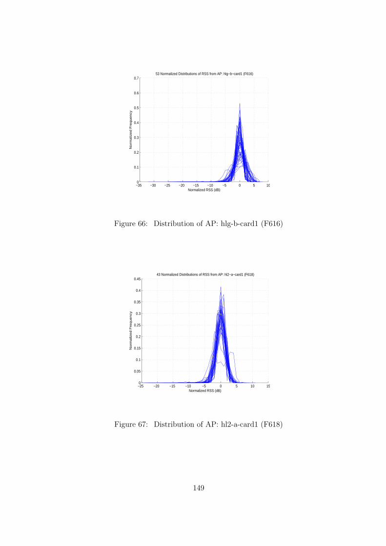
−35 −30 −25 −20 −15 −10 −5 0 5 100
0.1
0.2
0.3
0.4
0.5
0.6
0.7
Normalized RSS (dB)
No
rma
lize
d F
req
ue
ncy
53 Normalized Distributions of RSS from AP: hlg−b−card1 (F616)
Figure 66: Distribution of AP: hlg-b-card1 (F616)
−25 −20 −15 −10 −5 0 5 10 150
0.05
0.1
0.15
0.2
0.25
0.3
0.35
0.4
0.45
Normalized RSS (dB)
No
rma
lize
d F
req
ue
ncy
43 Normalized Distributions of RSS from AP: hl2−a−card1 (F618)
Figure 67: Distribution of AP: hl2-a-card1 (F618)
149
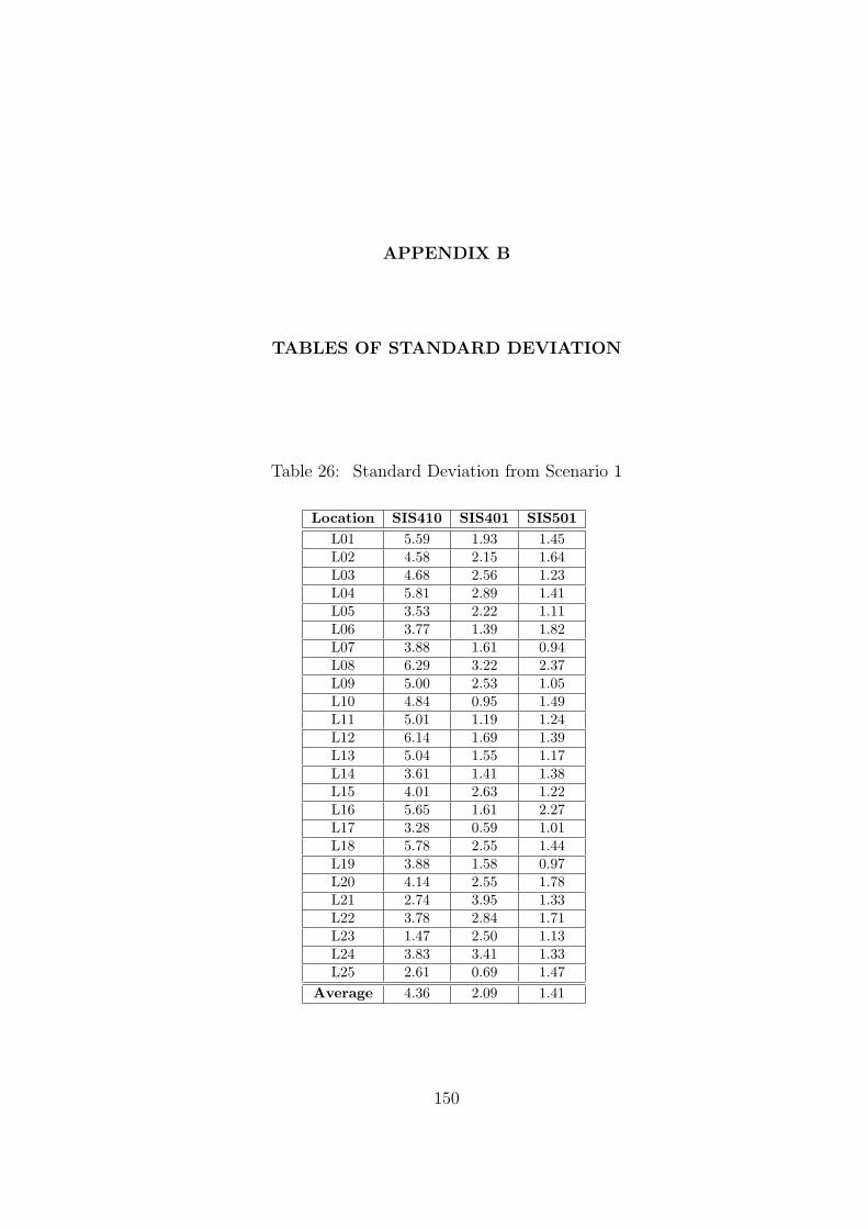
APPENDIX B
TABLES OF STANDARD DEVIATION
Table 26: Standard Deviation from Scenario 1
Location SIS410 SIS401 SIS501L01 5.59 1.93 1.45L02 4.58 2.15 1.64L03 4.68 2.56 1.23L04 5.81 2.89 1.41L05 3.53 2.22 1.11L06 3.77 1.39 1.82L07 3.88 1.61 0.94L08 6.29 3.22 2.37L09 5.00 2.53 1.05L10 4.84 0.95 1.49L11 5.01 1.19 1.24L12 6.14 1.69 1.39L13 5.04 1.55 1.17L14 3.61 1.41 1.38L15 4.01 2.63 1.22L16 5.65 1.61 2.27L17 3.28 0.59 1.01L18 5.78 2.55 1.44L19 3.88 1.58 0.97L20 4.14 2.55 1.78L21 2.74 3.95 1.33L22 3.78 2.84 1.71L23 1.47 2.50 1.13L24 3.83 3.41 1.33L25 2.61 0.69 1.47
Average 4.36 2.09 1.41
150
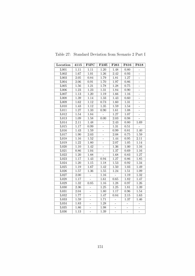
Table 27: Standard Deviation from Scenario 2 Part I
Location 4115 F5FC F23E F261 F616 F618L001 1.11 1.11 1.20 1.48 0.80 -L002 1.67 1.01 1.26 2.42 0.93 -L003 2.05 0.84 1.79 1.81 1.27 -L004 2.06 0.91 1.70 1.97 0.86 -L005 1.56 1.21 1.78 1.28 0.75 -L006 1.23 1.23 1.31 1.84 0.90 -L007 1.13 1.20 1.19 1.66 1.16 -L008 1.39 1.14 1.33 1.43 0.60 -L009 1.62 1.12 0.73 1.60 1.31 -L010 1.43 1.12 1.35 1.59 1.54 -L011 1.27 1.33 0.90 1.61 1.08 -L012 1.54 1.84 - 1.27 1.07 -L013 1.09 1.58 0.00 2.03 0.98 -L014 2.11 1.48 - 2.43 0.80 1.69L015 1.17 0.99 - 1.31 0.51 -L016 1.43 1.59 - 0.99 0.81 1.40L017 1.90 2.03 - 2.08 0.75 1.59L018 1.16 1.52 - 1.44 0.95 2.11L019 1.22 1.80 - 2.07 1.05 1.14L020 1.10 1.42 - 1.36 1.00 1.16L021 0.86 1.04 - 1.37 0.69 1.16L022 1.20 1.88 - 1.68 0.83 1.27L023 1.17 1.43 0.94 1.27 0.86 1.85L024 1.20 1.15 1.18 1.53 0.92 1.34L025 1.19 1.67 1.42 1.50 1.03 1.49L026 1.57 1.36 1.55 1.24 1.51 1.09L027 2.00 - 1.16 - 1.19 1.32L028 1.17 - 1.61 0.65 1.82 1.47L029 1.32 0.85 1.16 1.28 0.97 1.26L030 2.36 - 1.25 1.25 1.81 1.39L031 2.04 - 1.80 1.17 0.96 1.54L032 1.77 - 1.47 0.84 2.15 1.63L033 1.59 - 1.71 - 1.37 1.46L034 1.83 - 1.28 - - -L035 1.86 - 1.98 - - -L036 1.13 - 1.39 - - -
151
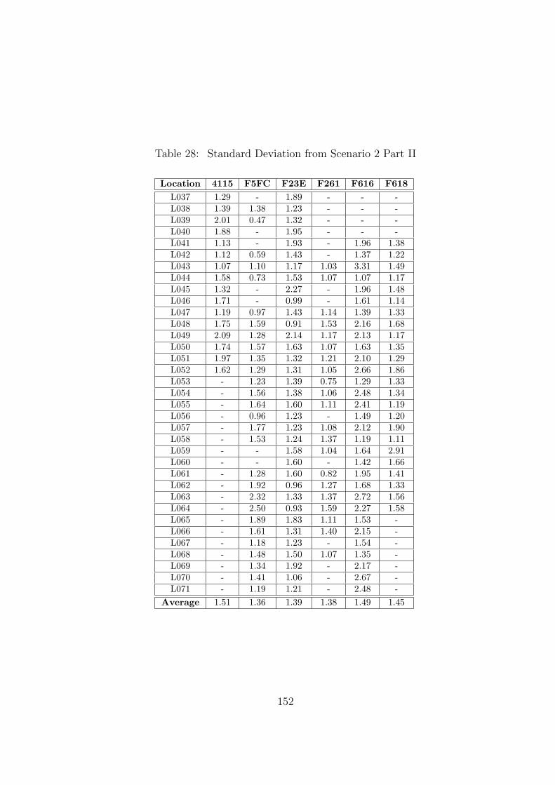
Table 28: Standard Deviation from Scenario 2 Part II
Location 4115 F5FC F23E F261 F616 F618L037 1.29 - 1.89 - - -L038 1.39 1.38 1.23 - - -L039 2.01 0.47 1.32 - - -L040 1.88 - 1.95 - - -L041 1.13 - 1.93 - 1.96 1.38L042 1.12 0.59 1.43 - 1.37 1.22L043 1.07 1.10 1.17 1.03 3.31 1.49L044 1.58 0.73 1.53 1.07 1.07 1.17L045 1.32 - 2.27 - 1.96 1.48L046 1.71 - 0.99 - 1.61 1.14L047 1.19 0.97 1.43 1.14 1.39 1.33L048 1.75 1.59 0.91 1.53 2.16 1.68L049 2.09 1.28 2.14 1.17 2.13 1.17L050 1.74 1.57 1.63 1.07 1.63 1.35L051 1.97 1.35 1.32 1.21 2.10 1.29L052 1.62 1.29 1.31 1.05 2.66 1.86L053 - 1.23 1.39 0.75 1.29 1.33L054 - 1.56 1.38 1.06 2.48 1.34L055 - 1.64 1.60 1.11 2.41 1.19L056 - 0.96 1.23 - 1.49 1.20L057 - 1.77 1.23 1.08 2.12 1.90L058 - 1.53 1.24 1.37 1.19 1.11L059 - - 1.58 1.04 1.64 2.91L060 - - 1.60 - 1.42 1.66L061 - 1.28 1.60 0.82 1.95 1.41L062 - 1.92 0.96 1.27 1.68 1.33L063 - 2.32 1.33 1.37 2.72 1.56L064 - 2.50 0.93 1.59 2.27 1.58L065 - 1.89 1.83 1.11 1.53 -L066 - 1.61 1.31 1.40 2.15 -L067 - 1.18 1.23 - 1.54 -L068 - 1.48 1.50 1.07 1.35 -L069 - 1.34 1.92 - 2.17 -L070 - 1.41 1.06 - 2.67 -L071 - 1.19 1.21 - 2.48 -
Average 1.51 1.36 1.39 1.38 1.49 1.45
152
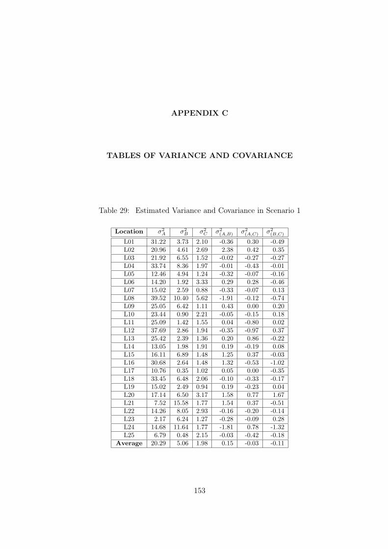
APPENDIX C
TABLES OF VARIANCE AND COVARIANCE
Table 29: Estimated Variance and Covariance in Scenario 1
Location σ2A σ2
B σ2C σ2
(A,B) σ2(A,C) σ2
(B,C)
L01 31.22 3.73 2.10 -0.36 0.30 -0.49L02 20.96 4.61 2.69 2.38 0.42 0.35L03 21.92 6.55 1.52 -0.02 -0.27 -0.27L04 33.74 8.36 1.97 -0.01 -0.43 -0.01L05 12.46 4.94 1.24 -0.32 -0.07 -0.16L06 14.20 1.92 3.33 0.29 0.28 -0.46L07 15.02 2.59 0.88 -0.33 -0.07 0.13L08 39.52 10.40 5.62 -1.91 -0.12 -0.74L09 25.05 6.42 1.11 0.43 0.00 0.20L10 23.44 0.90 2.21 -0.05 -0.15 0.18L11 25.09 1.42 1.55 0.04 -0.80 0.02L12 37.69 2.86 1.94 -0.35 -0.97 0.37L13 25.42 2.39 1.36 0.20 0.86 -0.22L14 13.05 1.98 1.91 0.19 -0.19 0.08L15 16.11 6.89 1.48 1.25 0.37 -0.03L16 30.68 2.64 1.48 1.32 -0.53 -1.02L17 10.76 0.35 1.02 0.05 0.00 -0.35L18 33.45 6.48 2.06 -0.10 -0.33 -0.17L19 15.02 2.49 0.94 0.19 -0.23 0.04L20 17.14 6.50 3.17 1.58 0.77 1.67L21 7.52 15.58 1.77 1.54 0.37 -0.51L22 14.26 8.05 2.93 -0.16 -0.20 -0.14L23 2.17 6.24 1.27 -0.28 -0.09 0.28L24 14.68 11.64 1.77 -1.81 0.78 -1.32L25 6.79 0.48 2.15 -0.03 -0.42 -0.18
Average 20.29 5.06 1.98 0.15 -0.03 -0.11
153
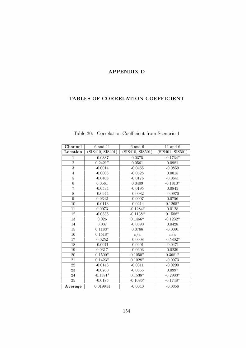
APPENDIX D
TABLES OF CORRELATION COEFFICIENT
Table 30: Correlation Coefficient from Scenario 1
Channel 6 and 11 6 and 6 11 and 6Location (SIS410, SIS401) (SIS410, SIS501) (SIS401, SIS501)
1 -0.0337 0.0375 -0.1734*2 0.2421* 0.0561 0.09813 -0.0014 -0.0465 -0.08594 -0.0003 -0.0528 0.00155 -0.0408 -0.0176 -0.06416 0.0561 0.0409 -0.1810*7 -0.0534 -0.0195 0.08458 -0.0944 -0.0082 -0.09709 0.0342 -0.0007 0.075610 -0.0113 -0.0214 0.1265*11 0.0073 -0.1284* 0.012812 -0.0336 -0.1138* 0.1588*13 0.026 0.1466* -0.1232*14 0.037 -0.0390 0.042815 0.1183* 0.0766 -0.009116 0.1518* n/a n/a17 0.0252 -0.0008 -0.5802*18 -0.0071 -0.0401 -0.047119 0.0317 -0.0603 0.023920 0.1500* 0.1050* 0.3681*21 0.1423* 0.1028* -0.097322 -0.0148 -0.0311 -0.029023 -0.0760 -0.0555 0.099724 -0.1381* 0.1538* -0.2903*25 -0.0185 -0.1086* -0.1748*
Average 0.019944 -0.0040 -0.0358
154
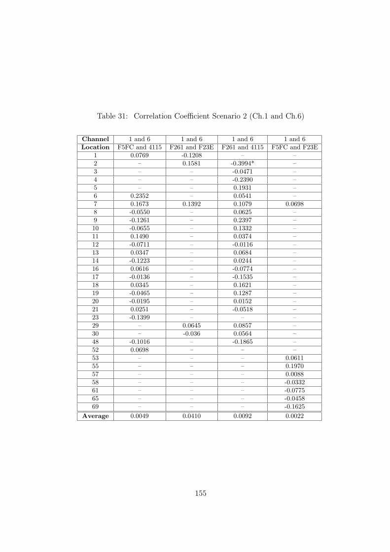
Table 31: Correlation Coefficient Scenario 2 (Ch.1 and Ch.6)
Channel 1 and 6 1 and 6 1 and 6 1 and 6Location F5FC and 4115 F261 and F23E F261 and 4115 F5FC and F23E
1 0.0769 -0.1208 – –2 – 0.1581 -0.3994* –3 – – -0.0471 –4 – – -0.2390 –5 – – 0.1931 –6 0.2352 – 0.0541 –7 0.1673 0.1392 0.1079 0.06988 -0.0550 – 0.0625 –9 -0.1261 – 0.2397 –10 -0.0655 – 0.1332 –11 0.1490 – 0.0374 –12 -0.0711 – -0.0116 –13 0.0347 – 0.0684 –14 -0.1223 – 0.0244 –16 0.0616 – -0.0774 –17 -0.0136 – -0.1535 –18 0.0345 – 0.1621 –19 -0.0465 – 0.1287 –20 -0.0195 – 0.0152 –21 0.0251 – -0.0518 –23 -0.1399 – – –29 – 0.0645 0.0857 –30 – -0.036 0.0564 –48 -0.1016 – -0.1865 –52 0.0698 – – –53 – – – 0.061155 – – – 0.197057 – – – 0.008858 – – – -0.033261 – – – -0.077565 – – – -0.045869 – – – -0.1625
Average 0.0049 0.0410 0.0092 0.0022
155
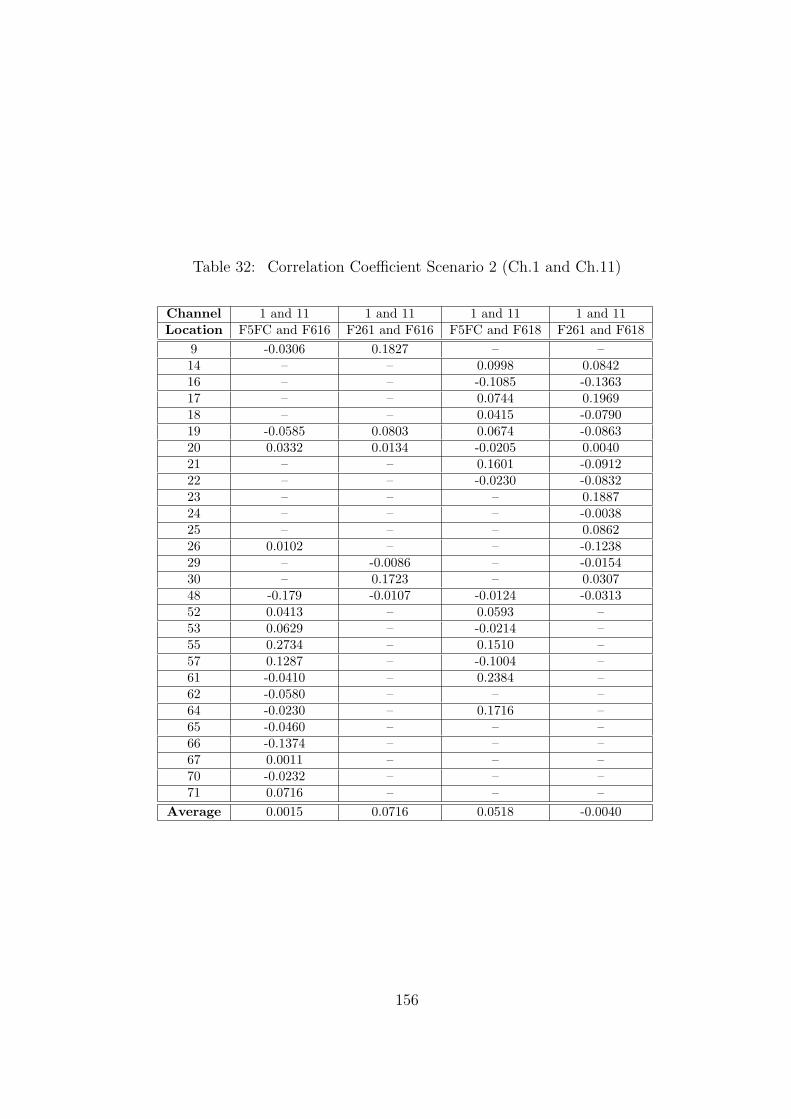
Table 32: Correlation Coefficient Scenario 2 (Ch.1 and Ch.11)
Channel 1 and 11 1 and 11 1 and 11 1 and 11Location F5FC and F616 F261 and F616 F5FC and F618 F261 and F618
9 -0.0306 0.1827 – –14 – – 0.0998 0.084216 – – -0.1085 -0.136317 – – 0.0744 0.196918 – – 0.0415 -0.079019 -0.0585 0.0803 0.0674 -0.086320 0.0332 0.0134 -0.0205 0.004021 – – 0.1601 -0.091222 – – -0.0230 -0.083223 – – – 0.188724 – – – -0.003825 – – – 0.086226 0.0102 – – -0.123829 – -0.0086 – -0.015430 – 0.1723 – 0.030748 -0.179 -0.0107 -0.0124 -0.031352 0.0413 – 0.0593 –53 0.0629 – -0.0214 –55 0.2734 – 0.1510 –57 0.1287 – -0.1004 –61 -0.0410 – 0.2384 –62 -0.0580 – – –64 -0.0230 – 0.1716 –65 -0.0460 – – –66 -0.1374 – – –67 0.0011 – – –70 -0.0232 – – –71 0.0716 – – –
Average 0.0015 0.0716 0.0518 -0.0040
156
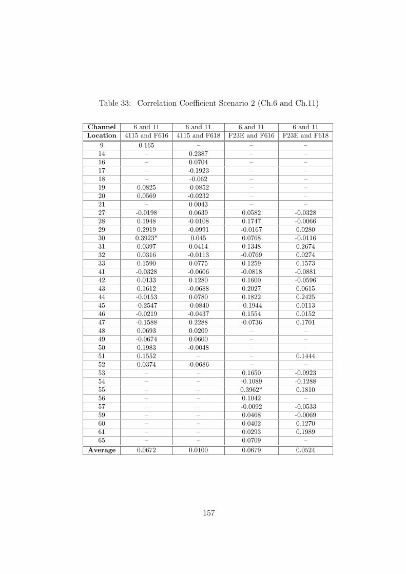
Table 33: Correlation Coefficient Scenario 2 (Ch.6 and Ch.11)
Channel 6 and 11 6 and 11 6 and 11 6 and 11Location 4115 and F616 4115 and F618 F23E and F616 F23E and F618
9 0.165 – – –14 – 0.2387 – –16 – 0.0704 – –17 – -0.1923 – –18 – -0.062 – –19 0.0825 -0.0852 – –20 0.0569 -0.0232 – –21 – 0.0043 – –27 -0.0198 0.0639 0.0582 -0.032828 0.1948 -0.0108 0.1747 -0.006629 0.2919 -0.0991 -0.0167 0.028030 0.3923* 0.045 0.0768 -0.011631 0.0397 0.0414 0.1348 0.267432 0.0316 -0.0113 -0.0769 0.027433 0.1590 0.0775 0.1259 0.157341 -0.0328 -0.0606 -0.0818 -0.088142 0.0133 0.1280 0.1600 -0.059643 0.1612 -0.0688 0.2027 0.061544 -0.0153 0.0780 0.1822 0.242545 -0.2547 -0.0840 -0.1944 0.011346 -0.0219 -0.0437 0.1554 0.015247 -0.1588 0.2288 -0.0736 0.170148 0.0693 0.0209 – –49 -0.0674 0.0600 – –50 0.1983 -0.0048 – –51 0.1552 – – 0.144452 0.0374 -0.0686 – –53 – – 0.1650 -0.092354 – – -0.1089 -0.128855 – – 0.3962* 0.181056 – – 0.1042 –57 – – -0.0092 -0.053359 – – 0.0468 -0.006960 – – 0.0402 0.127061 – – 0.0293 0.198965 – – 0.0709 –
Average 0.0672 0.0100 0.0679 0.0524
157
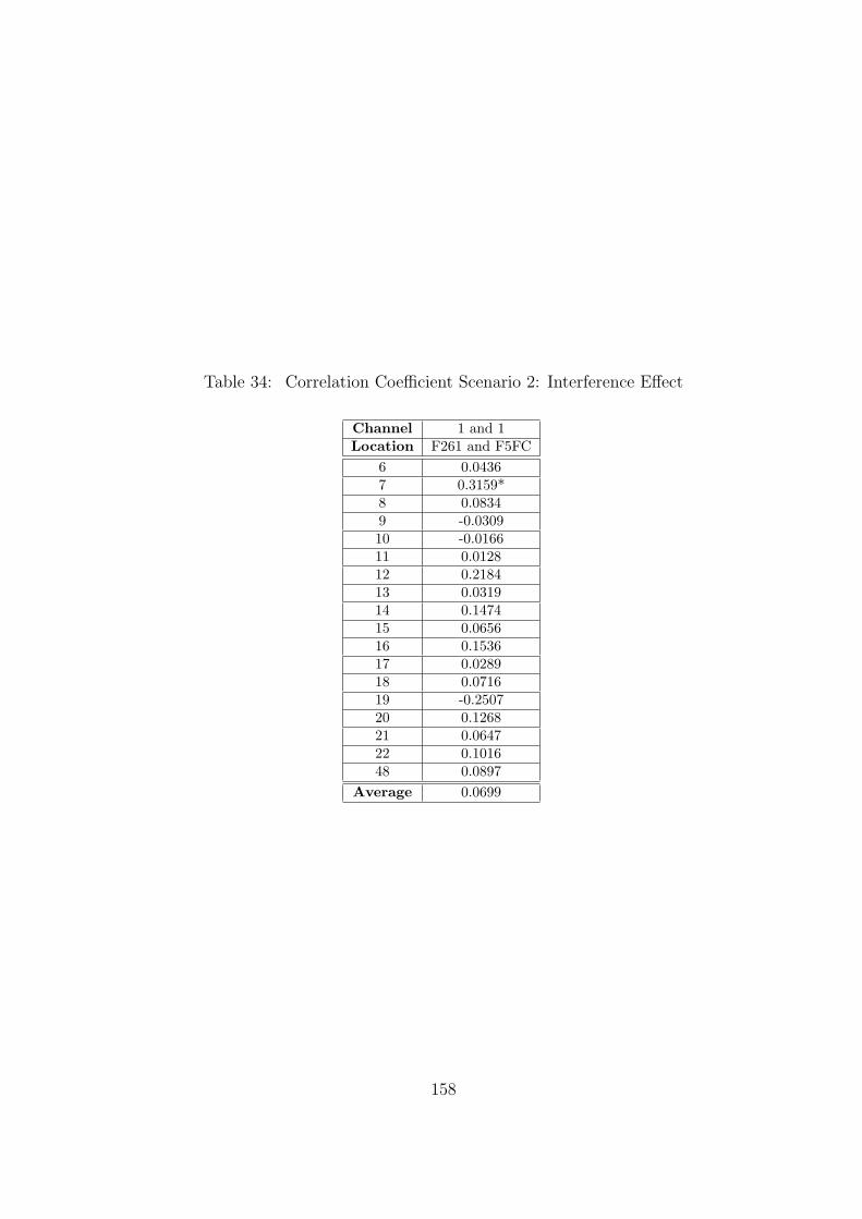
Table 34: Correlation Coefficient Scenario 2: Interference Effect
Channel 1 and 1Location F261 and F5FC
6 0.04367 0.3159*8 0.08349 -0.030910 -0.016611 0.012812 0.218413 0.031914 0.147415 0.065616 0.153617 0.028918 0.071619 -0.250720 0.126821 0.064722 0.101648 0.0897
Average 0.0699
158
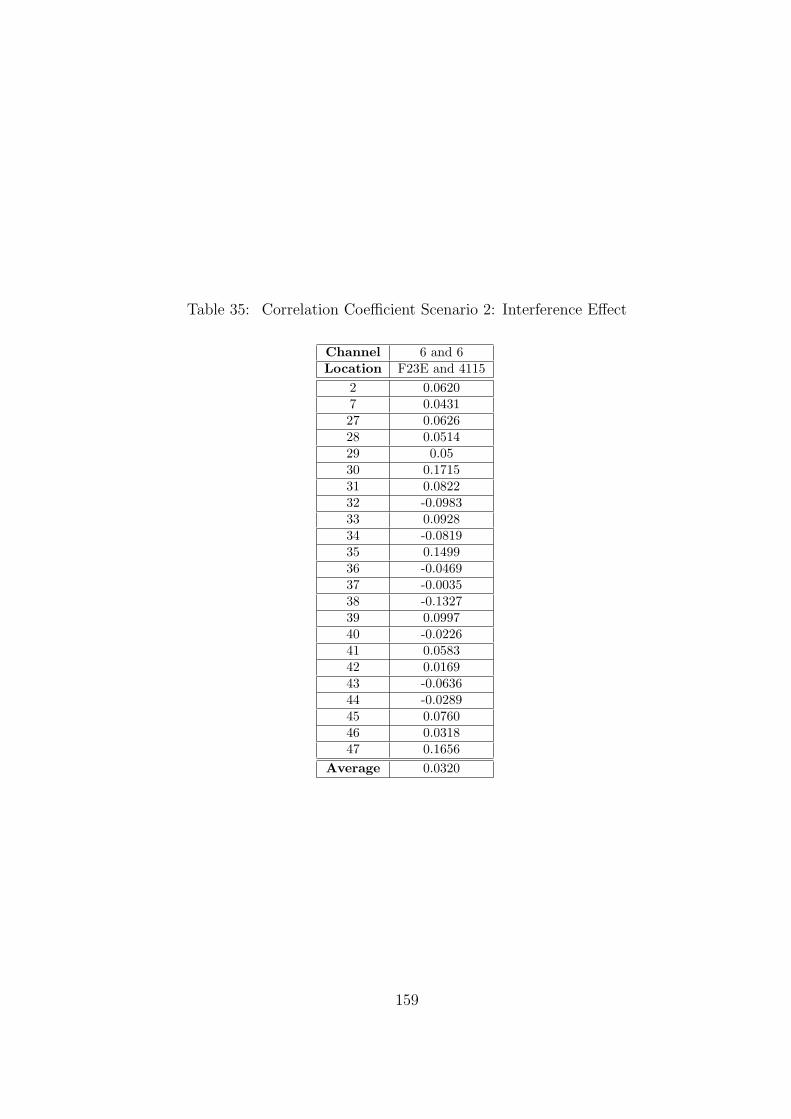
Table 35: Correlation Coefficient Scenario 2: Interference Effect
Channel 6 and 6Location F23E and 4115
2 0.06207 0.043127 0.062628 0.051429 0.0530 0.171531 0.082232 -0.098333 0.092834 -0.081935 0.149936 -0.046937 -0.003538 -0.132739 0.099740 -0.022641 0.058342 0.016943 -0.063644 -0.028945 0.076046 0.031847 0.1656
Average 0.0320
159
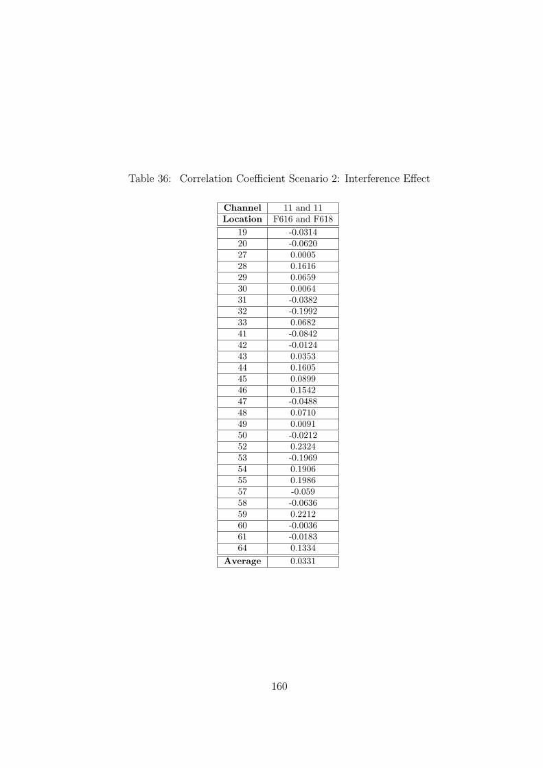
Table 36: Correlation Coefficient Scenario 2: Interference Effect
Channel 11 and 11Location F616 and F618
19 -0.031420 -0.062027 0.000528 0.161629 0.065930 0.006431 -0.038232 -0.199233 0.068241 -0.084242 -0.012443 0.035344 0.160545 0.089946 0.154247 -0.048848 0.071049 0.009150 -0.021252 0.232453 -0.196954 0.190655 0.198657 -0.05958 -0.063659 0.221260 -0.003661 -0.018364 0.1334
Average 0.0331
160
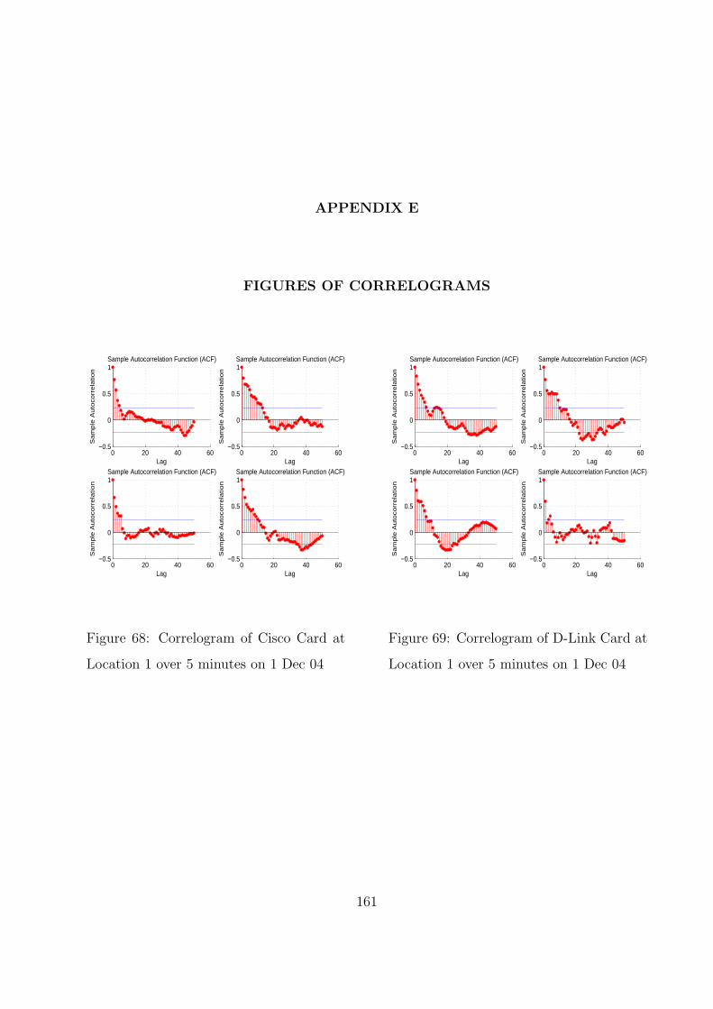
APPENDIX E
FIGURES OF CORRELOGRAMS
0 20 40 60−0.5
0
0.5
1
Lag
Sa
mp
le A
uto
corr
ela
tion
Sample Autocorrelation Function (ACF)
0 20 40 60−0.5
0
0.5
1
Lag
Sa
mp
le A
uto
corr
ela
tion
Sample Autocorrelation Function (ACF)
0 20 40 60−0.5
0
0.5
1
Lag
Sa
mp
le A
uto
corr
ela
tion
Sample Autocorrelation Function (ACF)
0 20 40 60−0.5
0
0.5
1
Lag
Sa
mp
le A
uto
corr
ela
tion
Sample Autocorrelation Function (ACF)
Figure 68: Correlogram of Cisco Card at
Location 1 over 5 minutes on 1 Dec 04
0 20 40 60−0.5
0
0.5
1
Lag
Sa
mp
le A
uto
corr
ela
tion
Sample Autocorrelation Function (ACF)
0 20 40 60−0.5
0
0.5
1
Lag
Sa
mp
le A
uto
corr
ela
tion
Sample Autocorrelation Function (ACF)
0 20 40 60−0.5
0
0.5
1
Lag
Sa
mp
le A
uto
corr
ela
tion
Sample Autocorrelation Function (ACF)
0 20 40 60−0.5
0
0.5
1
Lag
Sa
mp
le A
uto
corr
ela
tion
Sample Autocorrelation Function (ACF)
Figure 69: Correlogram of D-Link Card at
Location 1 over 5 minutes on 1 Dec 04
161
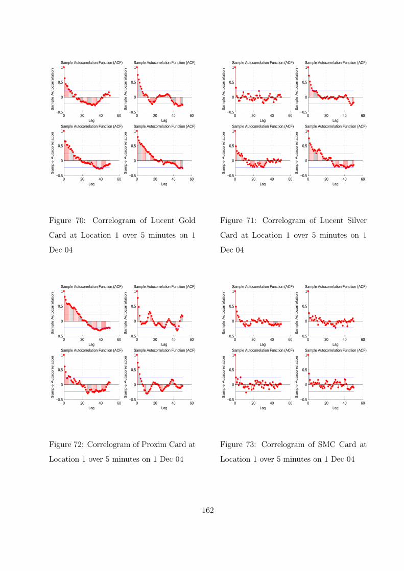
0 20 40 60−0.5
0
0.5
1
Lag
Sa
mp
le A
uto
corr
ela
tion
Sample Autocorrelation Function (ACF)
0 20 40 60−0.5
0
0.5
1
LagS
am
ple
Au
toco
rre
latio
n
Sample Autocorrelation Function (ACF)
0 20 40 60−0.5
0
0.5
1
Lag
Sa
mp
le A
uto
corr
ela
tion
Sample Autocorrelation Function (ACF)
0 20 40 60−0.5
0
0.5
1
Lag
Sa
mp
le A
uto
corr
ela
tion
Sample Autocorrelation Function (ACF)
Figure 70: Correlogram of Lucent Gold
Card at Location 1 over 5 minutes on 1
Dec 04
0 20 40 60−0.5
0
0.5
1
Lag
Sa
mp
le A
uto
corr
ela
tion
Sample Autocorrelation Function (ACF)
0 20 40 60−0.5
0
0.5
1
Lag
Sa
mp
le A
uto
corr
ela
tion
Sample Autocorrelation Function (ACF)
0 20 40 60−0.5
0
0.5
1
Lag
Sa
mp
le A
uto
corr
ela
tion
Sample Autocorrelation Function (ACF)
0 20 40 60−0.5
0
0.5
1
Lag
Sa
mp
le A
uto
corr
ela
tion
Sample Autocorrelation Function (ACF)
Figure 71: Correlogram of Lucent Silver
Card at Location 1 over 5 minutes on 1
Dec 04
0 20 40 60−0.5
0
0.5
1
Lag
Sa
mp
le A
uto
corr
ela
tion
Sample Autocorrelation Function (ACF)
0 20 40 60−0.5
0
0.5
1
Lag
Sa
mp
le A
uto
corr
ela
tion
Sample Autocorrelation Function (ACF)
0 20 40 60−0.5
0
0.5
1
Lag
Sa
mp
le A
uto
corr
ela
tion
Sample Autocorrelation Function (ACF)
0 20 40 60−0.5
0
0.5
1
Lag
Sa
mp
le A
uto
corr
ela
tion
Sample Autocorrelation Function (ACF)
Figure 72: Correlogram of Proxim Card at
Location 1 over 5 minutes on 1 Dec 04
0 20 40 60−0.5
0
0.5
1
Lag
Sa
mp
le A
uto
corr
ela
tion
Sample Autocorrelation Function (ACF)
0 20 40 60−0.5
0
0.5
1
Lag
Sa
mp
le A
uto
corr
ela
tion
Sample Autocorrelation Function (ACF)
0 20 40 60−0.5
0
0.5
1
Lag
Sa
mp
le A
uto
corr
ela
tion
Sample Autocorrelation Function (ACF)
0 20 40 60−0.5
0
0.5
1
Lag
Sa
mp
le A
uto
corr
ela
tion
Sample Autocorrelation Function (ACF)
Figure 73: Correlogram of SMC Card at
Location 1 over 5 minutes on 1 Dec 04
162
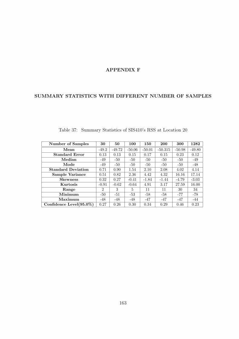
APPENDIX F
SUMMARY STATISTICS WITH DIFFERENT NUMBER OF SAMPLES
Table 37: Summary Statistics of SIS410’s RSS at Location 20
Number of Samples 30 50 100 150 200 300 1282Mean -49.2 -49.72 -50.06 -50.01 -50.315 -50.98 -49.80
Standard Error 0.13 0.13 0.15 0.17 0.15 0.23 0.12Median -49 -50 -50 -50 -50 -50 -49Mode -49 -50 -50 -50 -50 -50 -48
Standard Deviation 0.71 0.90 1.54 2.10 2.08 4.02 4.14Sample Variance 0.51 0.82 2.36 4.42 4.32 16.16 17.14
Skewness 0.32 0.27 -0.41 -1.84 -1.44 -4.79 -3.03Kurtosis -0.91 -0.62 -0.64 4.91 3.17 27.59 16.00Range 2 3 5 11 11 30 34
Minimum -50 -51 -53 -58 -58 -77 -78Maximum -48 -48 -48 -47 -47 -47 -44
Confidence Level(95.0%) 0.27 0.26 0.30 0.34 0.29 0.46 0.23
163
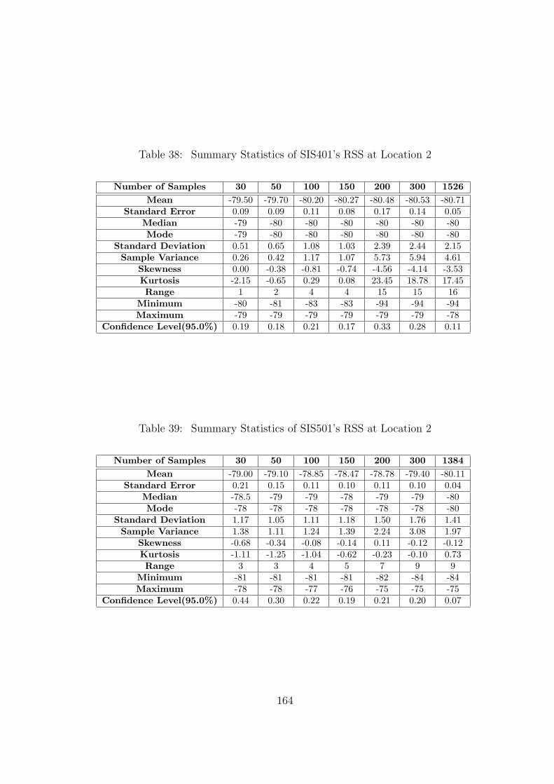
Table 38: Summary Statistics of SIS401’s RSS at Location 2
Number of Samples 30 50 100 150 200 300 1526Mean -79.50 -79.70 -80.20 -80.27 -80.48 -80.53 -80.71
Standard Error 0.09 0.09 0.11 0.08 0.17 0.14 0.05Median -79 -80 -80 -80 -80 -80 -80Mode -79 -80 -80 -80 -80 -80 -80
Standard Deviation 0.51 0.65 1.08 1.03 2.39 2.44 2.15Sample Variance 0.26 0.42 1.17 1.07 5.73 5.94 4.61
Skewness 0.00 -0.38 -0.81 -0.74 -4.56 -4.14 -3.53Kurtosis -2.15 -0.65 0.29 0.08 23.45 18.78 17.45Range 1 2 4 4 15 15 16
Minimum -80 -81 -83 -83 -94 -94 -94Maximum -79 -79 -79 -79 -79 -79 -78
Confidence Level(95.0%) 0.19 0.18 0.21 0.17 0.33 0.28 0.11
Table 39: Summary Statistics of SIS501’s RSS at Location 2
Number of Samples 30 50 100 150 200 300 1384Mean -79.00 -79.10 -78.85 -78.47 -78.78 -79.40 -80.11
Standard Error 0.21 0.15 0.11 0.10 0.11 0.10 0.04Median -78.5 -79 -79 -78 -79 -79 -80Mode -78 -78 -78 -78 -78 -78 -80
Standard Deviation 1.17 1.05 1.11 1.18 1.50 1.76 1.41Sample Variance 1.38 1.11 1.24 1.39 2.24 3.08 1.97
Skewness -0.68 -0.34 -0.08 -0.14 0.11 -0.12 -0.12Kurtosis -1.11 -1.25 -1.04 -0.62 -0.23 -0.10 0.73Range 3 3 4 5 7 9 9
Minimum -81 -81 -81 -81 -82 -84 -84Maximum -78 -78 -77 -76 -75 -75 -75
Confidence Level(95.0%) 0.44 0.30 0.22 0.19 0.21 0.20 0.07
164
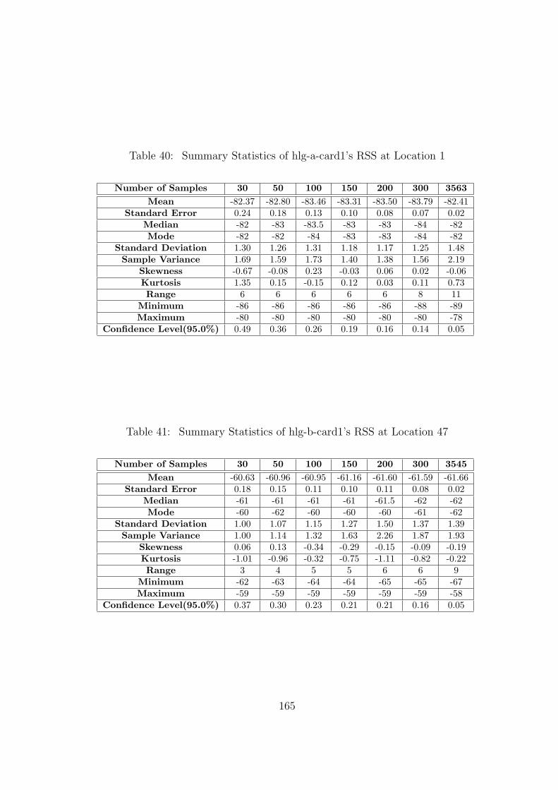
Table 40: Summary Statistics of hlg-a-card1’s RSS at Location 1
Number of Samples 30 50 100 150 200 300 3563Mean -82.37 -82.80 -83.46 -83.31 -83.50 -83.79 -82.41
Standard Error 0.24 0.18 0.13 0.10 0.08 0.07 0.02Median -82 -83 -83.5 -83 -83 -84 -82Mode -82 -82 -84 -83 -83 -84 -82
Standard Deviation 1.30 1.26 1.31 1.18 1.17 1.25 1.48Sample Variance 1.69 1.59 1.73 1.40 1.38 1.56 2.19
Skewness -0.67 -0.08 0.23 -0.03 0.06 0.02 -0.06Kurtosis 1.35 0.15 -0.15 0.12 0.03 0.11 0.73Range 6 6 6 6 6 8 11
Minimum -86 -86 -86 -86 -86 -88 -89Maximum -80 -80 -80 -80 -80 -80 -78
Confidence Level(95.0%) 0.49 0.36 0.26 0.19 0.16 0.14 0.05
Table 41: Summary Statistics of hlg-b-card1’s RSS at Location 47
Number of Samples 30 50 100 150 200 300 3545Mean -60.63 -60.96 -60.95 -61.16 -61.60 -61.59 -61.66
Standard Error 0.18 0.15 0.11 0.10 0.11 0.08 0.02Median -61 -61 -61 -61 -61.5 -62 -62Mode -60 -62 -60 -60 -60 -61 -62
Standard Deviation 1.00 1.07 1.15 1.27 1.50 1.37 1.39Sample Variance 1.00 1.14 1.32 1.63 2.26 1.87 1.93
Skewness 0.06 0.13 -0.34 -0.29 -0.15 -0.09 -0.19Kurtosis -1.01 -0.96 -0.32 -0.75 -1.11 -0.82 -0.22Range 3 4 5 5 6 6 9
Minimum -62 -63 -64 -64 -65 -65 -67Maximum -59 -59 -59 -59 -59 -59 -58
Confidence Level(95.0%) 0.37 0.30 0.23 0.21 0.21 0.16 0.05
165
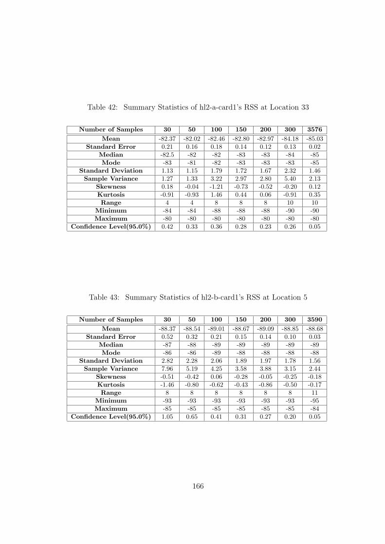
Table 42: Summary Statistics of hl2-a-card1’s RSS at Location 33
Number of Samples 30 50 100 150 200 300 3576Mean -82.37 -82.02 -82.46 -82.80 -82.97 -84.18 -85.03
Standard Error 0.21 0.16 0.18 0.14 0.12 0.13 0.02Median -82.5 -82 -82 -83 -83 -84 -85Mode -83 -81 -82 -83 -83 -83 -85
Standard Deviation 1.13 1.15 1.79 1.72 1.67 2.32 1.46Sample Variance 1.27 1.33 3.22 2.97 2.80 5.40 2.13
Skewness 0.18 -0.04 -1.21 -0.73 -0.52 -0.20 0.12Kurtosis -0.91 -0.93 1.46 0.44 0.06 -0.91 0.35Range 4 4 8 8 8 10 10
Minimum -84 -84 -88 -88 -88 -90 -90Maximum -80 -80 -80 -80 -80 -80 -80
Confidence Level(95.0%) 0.42 0.33 0.36 0.28 0.23 0.26 0.05
Table 43: Summary Statistics of hl2-b-card1’s RSS at Location 5
Number of Samples 30 50 100 150 200 300 3590Mean -88.37 -88.54 -89.01 -88.67 -89.09 -88.85 -88.68
Standard Error 0.52 0.32 0.21 0.15 0.14 0.10 0.03Median -87 -88 -89 -89 -89 -89 -89Mode -86 -86 -89 -88 -88 -88 -88
Standard Deviation 2.82 2.28 2.06 1.89 1.97 1.78 1.56Sample Variance 7.96 5.19 4.25 3.58 3.88 3.15 2.44
Skewness -0.51 -0.42 0.06 -0.28 -0.05 -0.25 -0.18Kurtosis -1.46 -0.80 -0.62 -0.43 -0.86 -0.50 -0.17Range 8 8 8 8 8 8 11
Minimum -93 -93 -93 -93 -93 -93 -95Maximum -85 -85 -85 -85 -85 -85 -84
Confidence Level(95.0%) 1.05 0.65 0.41 0.31 0.27 0.20 0.05
166
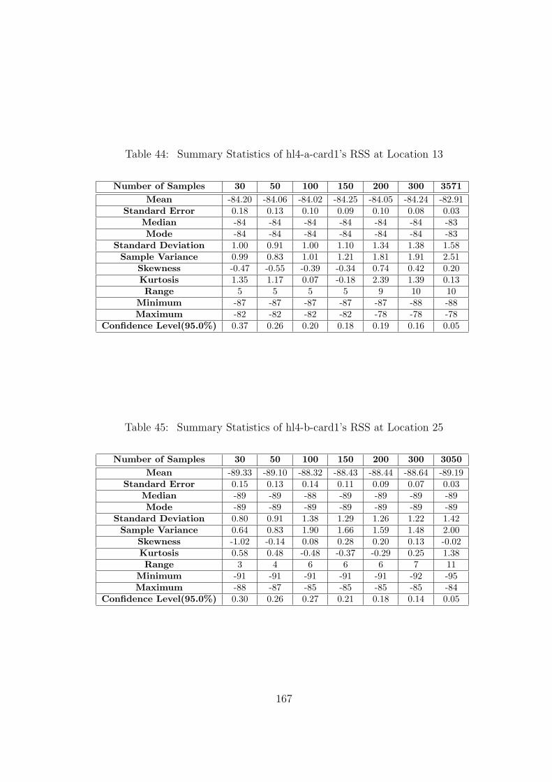
Table 44: Summary Statistics of hl4-a-card1’s RSS at Location 13
Number of Samples 30 50 100 150 200 300 3571Mean -84.20 -84.06 -84.02 -84.25 -84.05 -84.24 -82.91
Standard Error 0.18 0.13 0.10 0.09 0.10 0.08 0.03Median -84 -84 -84 -84 -84 -84 -83Mode -84 -84 -84 -84 -84 -84 -83
Standard Deviation 1.00 0.91 1.00 1.10 1.34 1.38 1.58Sample Variance 0.99 0.83 1.01 1.21 1.81 1.91 2.51
Skewness -0.47 -0.55 -0.39 -0.34 0.74 0.42 0.20Kurtosis 1.35 1.17 0.07 -0.18 2.39 1.39 0.13Range 5 5 5 5 9 10 10
Minimum -87 -87 -87 -87 -87 -88 -88Maximum -82 -82 -82 -82 -78 -78 -78
Confidence Level(95.0%) 0.37 0.26 0.20 0.18 0.19 0.16 0.05
Table 45: Summary Statistics of hl4-b-card1’s RSS at Location 25
Number of Samples 30 50 100 150 200 300 3050Mean -89.33 -89.10 -88.32 -88.43 -88.44 -88.64 -89.19
Standard Error 0.15 0.13 0.14 0.11 0.09 0.07 0.03Median -89 -89 -88 -89 -89 -89 -89Mode -89 -89 -89 -89 -89 -89 -89
Standard Deviation 0.80 0.91 1.38 1.29 1.26 1.22 1.42Sample Variance 0.64 0.83 1.90 1.66 1.59 1.48 2.00
Skewness -1.02 -0.14 0.08 0.28 0.20 0.13 -0.02Kurtosis 0.58 0.48 -0.48 -0.37 -0.29 0.25 1.38Range 3 4 6 6 6 7 11
Minimum -91 -91 -91 -91 -91 -92 -95Maximum -88 -87 -85 -85 -85 -85 -84
Confidence Level(95.0%) 0.30 0.26 0.27 0.21 0.18 0.14 0.05
167

APPENDIX G
FLOWCHARTS OF INDOOR POSITIONING PROTOTYPE
168
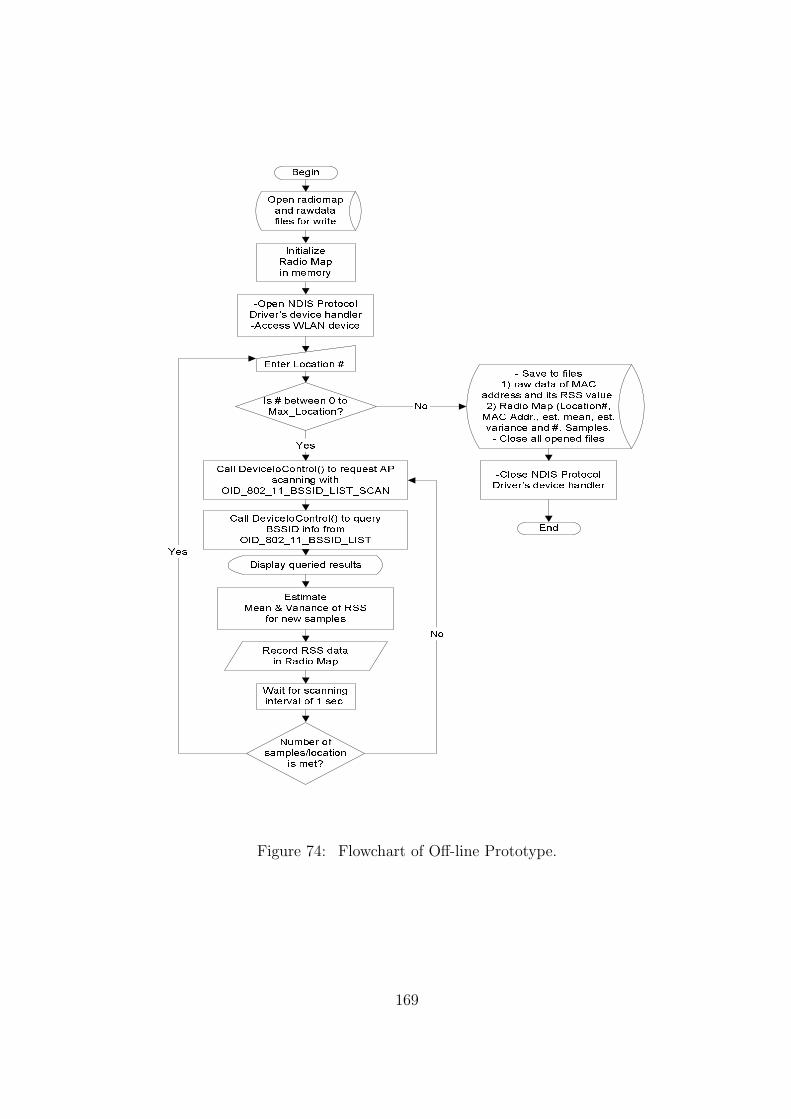
BeginEnter Location #.Call DeviceIoControl() to request APscanning withOID_802_11_BSSID_LIST_SCANEstimateMean & Variance of RSSfor new samplesNumber ofsamples/locationis met?
- Save to files1) raw data of MACaddress and its RSS value.2) Radio Map (Location#,MAC Addr., est. mean, est.variance and #. Samples.- Close all opened filesIs # between 0 toMax_Location?Open radiomapand rawdatafiles for write-Open NDIS ProtocolDriver’s device handler-Access WLAN device
Wait for scanninginterval of 1 sec.Call DeviceIoControl() to queryBSSID info fromOID_802_11_BSSID_LISTDisplay queried resultsRecord RSS datain Radio Map
YesNoYes
No End-Close NDIS ProtocolDriver’s device handlerInitializeRadio Mapin memory
Figure 74: Flowchart of Off-line Prototype.
169
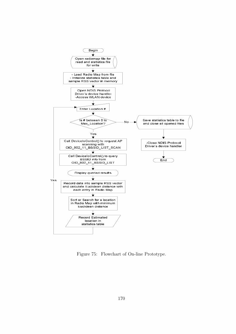
BeginEnter Location #.Call DeviceIoControl() to request APscanning withOID_802_11_BSSID_LIST_SCANRecord data into sample RSS vectorand calculate Euclidean distance witheach entry in Radio Map
Save statistics table to fileand close all opened filesIs # between 0 toMax_Location?Open radiomap file forread and statistics filefor write-Open NDIS ProtocolDriver’s device handler-Access WLAN device
Call DeviceIoControl() to queryBSSID info fromOID_802_11_BSSID_LISTDisplay queried resultsRecord Estimatedlocation instatistics table
YesYes
No- Load Radio Map from file- Initialize statistics table andsample RSS vector in memory
End-Close NDIS ProtocolDriver’s device handlerSort or Search for a locationin Radio Map with minimumEuclidean distance
Figure 75: Flowchart of On-line Prototype.
170

APPENDIX H
LOCATION FINGERPRINTS OF PROTOTYPE’S EXPERIMENT
171
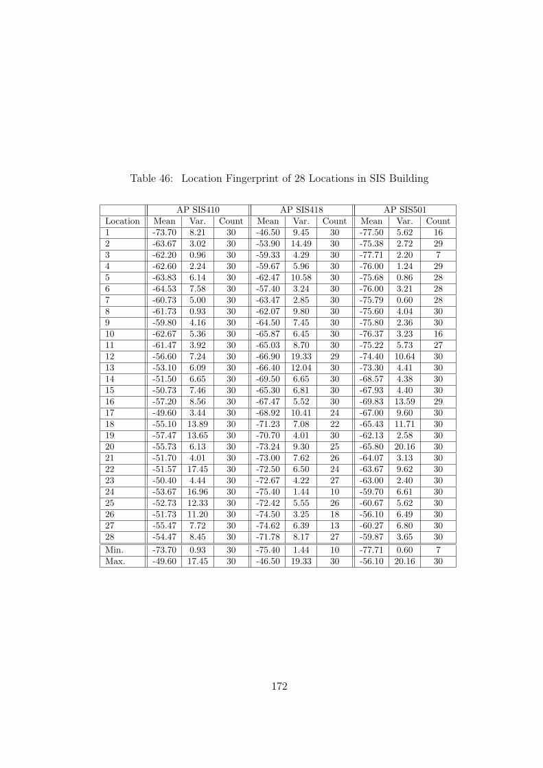
Table 46: Location Fingerprint of 28 Locations in SIS Building
AP SIS410 AP SIS418 AP SIS501Location Mean Var. Count Mean Var. Count Mean Var. Count1 -73.70 8.21 30 -46.50 9.45 30 -77.50 5.62 162 -63.67 3.02 30 -53.90 14.49 30 -75.38 2.72 293 -62.20 0.96 30 -59.33 4.29 30 -77.71 2.20 74 -62.60 2.24 30 -59.67 5.96 30 -76.00 1.24 295 -63.83 6.14 30 -62.47 10.58 30 -75.68 0.86 286 -64.53 7.58 30 -57.40 3.24 30 -76.00 3.21 287 -60.73 5.00 30 -63.47 2.85 30 -75.79 0.60 288 -61.73 0.93 30 -62.07 9.80 30 -75.60 4.04 309 -59.80 4.16 30 -64.50 7.45 30 -75.80 2.36 3010 -62.67 5.36 30 -65.87 6.45 30 -76.37 3.23 1611 -61.47 3.92 30 -65.03 8.70 30 -75.22 5.73 2712 -56.60 7.24 30 -66.90 19.33 29 -74.40 10.64 3013 -53.10 6.09 30 -66.40 12.04 30 -73.30 4.41 3014 -51.50 6.65 30 -69.50 6.65 30 -68.57 4.38 3015 -50.73 7.46 30 -65.30 6.81 30 -67.93 4.40 3016 -57.20 8.56 30 -67.47 5.52 30 -69.83 13.59 2917 -49.60 3.44 30 -68.92 10.41 24 -67.00 9.60 3018 -55.10 13.89 30 -71.23 7.08 22 -65.43 11.71 3019 -57.47 13.65 30 -70.70 4.01 30 -62.13 2.58 3020 -55.73 6.13 30 -73.24 9.30 25 -65.80 20.16 3021 -51.70 4.01 30 -73.00 7.62 26 -64.07 3.13 3022 -51.57 17.45 30 -72.50 6.50 24 -63.67 9.62 3023 -50.40 4.44 30 -72.67 4.22 27 -63.00 2.40 3024 -53.67 16.96 30 -75.40 1.44 10 -59.70 6.61 3025 -52.73 12.33 30 -72.42 5.55 26 -60.67 5.62 3026 -51.73 11.20 30 -74.50 3.25 18 -56.10 6.49 3027 -55.47 7.72 30 -74.62 6.39 13 -60.27 6.80 3028 -54.47 8.45 30 -71.78 8.17 27 -59.87 3.65 30Min. -73.70 0.93 30 -75.40 1.44 10 -77.71 0.60 7Max. -49.60 17.45 30 -46.50 19.33 30 -56.10 20.16 30
172
BIBLIOGRAPHY
[1] T. P. Moran and P. Dourish, “Introduction to this special issue on context-aware com-puting,” Human-Computer Interaction, vol. 16, no. 2,3,& 4, pp. 87–95, 2001.
[2] M. Weiser, “Some computer science issues in ubiquitous computing,” Communicationsof the ACM, vol. 36, no. 7, pp. 75–84, July 1993.
[3] “Pervasive computing 2001: Major IT industry conference,” WebPage, InformationTechnology Laboratory, National Institute of Standards and Technology (NIST), May2001. [Online]. Available: http://www.nist.gov/pc2001/
[4] P. Krishnamurthy, “Position location in mobile environments,” in Proc. NSF Workshopon Context-Aware Mobile Database Management (CAMM), Providence, RI, Jan. 2002.
[5] T. S. Rappaport, J. H. Reed, and B. D. Woerner, “Position location using wirelesscommunications on highways of the future,” IEEE Commun. Mag., vol. 34, no. 10, pp.33–41, Oct. 1996.
[6] K. Pahlavan, X. Li, and J. P. Makela, “Indoor geolocation science and technology,”IEEE Commun. Mag., vol. 40, no. 2, pp. 112–118, Feb. 2002.
[7] J. Hightower and G. Borriello, “Location systems for ubiquitous computing,” IEEEComputer, vol. 34, no. 8, pp. 57–66, Aug. 2001.
[8] A. M. Ladd, K. E. Bekris, G. Marceau, A. Rudys, L. E. Kavraki, and D. S. Wallach,“Robotics-based location sensing using wireless ethernet,” in Proc. ACM InternationalConference on Mobile Computing and Networking (MOBICOM’02), 2002, pp. 227–238.
[9] I. Ramani, R. Bharadwaja, and P. V. Rangan, “Location tracking for media appliancesin wireless home networks,” in Proc. International Conference on Multimedia and Expo(ICME’03), July 2003, pp. 769–772.
[10] G. M. Djuknic and R. E. Richton, “Geolocation and assisted GPS,” IEEE Computer,vol. 34, no. 2, pp. 123–125, Feb. 2001.
[11] Merriam-Webster, Merriam-Webster’s Collegiate Dictionary, 11st ed. Springfield, MA:Merriam-Webster Inc., July 2003.
173
[12] B. Sklar, “Rayleigh fading channels in mobile digital communication systems: I. char-acterization,” IEEE Commun. Mag., vol. 35, no. 7, pp. 90–100, July 1997.
[13] P. Bahl and V. N. Padmanabhan, “RADAR: an in-building RF-based user locationand tracking system,” in Proc. IEEE Nineteenth Annual Joint Conference of the IEEEComputer and Communications Societies (INFOCOM’00), Tel Aviv, Israel, Mar. 2000,pp. 775–784.
[14] J. A. Tauber, “Location systems for pervasive computing,” Area Exam Report, Massa-chusetts Institute of Technology, Aug. 2002.
[15] M. J. Meyer and et al., “Wireless enhanced 9-1-1 service – making it a reality,” BellLabs Technical Journal, 1996, autumn.
[16] P. Prasithsangaree, P. Krishnamurthy, and P. K. Chrysanthis, “On indoor positionlocation with wireless LANs,” in Proc. IEEE International Symposium on Personal,Indoor, and Mobile Radio Communications (PIMRC’02), Lisbon, Portugal, Sept. 2002.
[17] Z. Xiang, S. Song, J. Chen, H. Wang, J. Huang, and X. Gao, “A wireless LAN-basedindoor positioning technology,” IBM Journal of Research and Development, vol. 48, no.5/6, pp. 617–626, Sept./Nov. 2004.
[18] M. A. Youssef, A. Agrawala, and A. U. Shankar, “WLAN location determination viaclustering and probability distributions,” in Proc. IEEE International Conference onPervasive Computing and Communications (PerCom’03), Dallas-Fort Worth, TX, Mar.23–26, 2003, pp. 23–26.
[19] A. Smailagic and D. Kogan, “Location sensing and privacy in a context-aware computingenvironment,” IEEE Wireless Commun. Mag., vol. 9, no. 5, pp. 1536–1284, Oct. 2002.
[20] P. Castro, P. Chiu, T. Kremenek, and R. Muntz, “A probabilistic room location ser-vice for wireless networked environments,” in Proc. ACM International Conference onUbiquitous Computing (UbiComp’01), Atlanta, GA, Sept. 2001.
[21] Ekahau Positioning Engine 2.1, User Guide, Ekahau, Inc., 2003. [Online]. Available:http://www.ekahau.com
[22] R. Battiti, M. Brunato, and A. Villani, “Statistical learning theory for locationfingerprinting in wireless lans,” Technical Report, Oct. 2002. [Online]. Available:http://rtm.science.unitn.it/∼battiti/archive/86.pdf
[23] T. Roos, P. Myllymaki, H. Tirri, P. Misikangas, and J. Sievanen, “A probabilistic ap-proach to wlan user location estimation,” International Journal of Wireless InformationNetworks, vol. 9, no. 3, pp. 155–164, July 2002.
[24] J. Hightower, B. Brumitt, and G. Borriello, “The location stack: A layered modelfor location in ubiquitous computing,” in Proc. IEEE Workshop on Mobile ComputingSystems & Applications (WMCSA’02), Callicoon, NY, June 2002, pp. 22–28.
174
[25] R. Want, A. Hopper, V. Falcao, and J. Gibbons, “The active badge location system,”ACM Transactions on Information Systems, vol. 40, no. 1, pp. 91–102, Jan. 1992.
[26] A. Harter, A. Hopper, P. Steggles, A. Ward, and P. Webster, “The anatomy of a context-aware application,” in Proc. ACM International Conference on Mobile Computing andNetworking (MOBICOM’99), Seattle, WA, Aug. 1999.
[27] N. B. Priyantha, A. Chakraborty, and H. Balakrishnan, “The cricket location-supportsystem,” in Proc. ACM International Conference on Mobile Computing and Networking(MOBICOM’00), Boston, MA, Aug. 2000, pp. 32–43.
[28] V. Zeimpekis, G. M. Giaglis, and G. Lekakos, “A taxonomy of indoor and outdoorpositioning techniques for mobile location services,” Journal of ACM Special InterestGroup on Electronic Commerce, vol. 3, pp. 19–27, 2002.
[29] J. Hightower, R. Want, and G. Borriello, “SpotON: An indoor 3D locationsensing technology based on RF signal strength,” University of Washington,Seattle, WA, Techical Report UW CSE 2000-02-02, Feb. 2000. [Online]. Avail-able: http://seattle.intel-research.net/people/jhightower/pubs/hightower2000indoor/hightower2000indoor.pdf
[30] J. Werb and C. Lanzl, “Designing a positioning system for finding things and peopleindoors,” IEEE Spectr., vol. 35, no. 9, pp. 71–78, Sept. 1998.
[31] S. Saha, K. Chaudhuri, D. Sanghi, and P. Bhagwat, “Location determination of a mobiledevice using ieee 802.11b access point signals,” in Proc. IEEE Wireless Communicationsand Networking Conference (WCNC’03), New Orleans, LA, Mar. 2003, pp. 1987–1992.
[32] J. Small, A. Smailagic, and D. P. Siewiorek, “Determining user location for contextaware computing through the use of a wireless lan infrastructure,” Online, Dec. 2000.[Online]. Available: http://www-2.cs.cmu.edu/∼aura/docdir/small00.pdf
[33] R. Jain, The Art of Computer Systems Performance Analysis: Techniques for Experi-mental Design, Measurement, Simulation, and Modeling. New York, NY: John Wiley& Sons, 1991.
[34] J. T. Tou and R. C. Gonzalez, Pattern Recognition Principles, 2nd ed. Reading, MA:Addison-Wesley, 1974.
[35] M. Pardo and G. Sberveglieri, “Learning from data: A tutorial with emphasis on modernpattern recognition methods,” IEEE Sensors J., vol. 2, no. 3, pp. 203–217, June 2002.
[36] P. E. Black, “Dictionary of algorithms and data structures,” Information TechnologyLaboratory, National Institute of Standards and Technology (NIST), 2005.
[37] A. K. Jain, R. P. W. Duin, and J. Mao, “Statistical pattern recognition: A review,”IEEE Trans. Pattern Anal. Machine Intell., vol. 22, no. 1, pp. 4–37, Jan. 2000.
175
[38] R. O. Duda, P. E. Hart, and D. G. Stork, Pattern Classification, 2nd ed. New York,NY: Wiley-Interscience, 2000.
[39] F. Rosenblatt, “The perceptron: A probabilistic model for information storage and or-ganization in the brain,” Cornell Aeronautical Laboratory, Psychological Review, vol. 65,no. 6, pp. 386–408, 1958.
[40] R. Battiti, “Location-aware computing: a neural network model for determininglocation in wireless lans,” Universita degli Studi di Trento, Tech. Rep. DIT-0083, Feb.2002. [Online]. Available: http://rtm.science.unitn.it/∼battiti/archive/83.pdf
[41] M. A. Youssef and A. Agrawala, “On the optimality of WLAN location determinationsystems,” University of Maryland, College Park, MD, Technical Report CS-TR 4459,Mar. 2003. [Online]. Available: http://www.cs.umd.edu/∼moustafa/papers/opt tr.pdf
[42] V. N. Vapnik, Statistical Learning Theory. New York, NY: John Wiley & Sons, Sept.1998.
[43] E. W. Weisstein, “Hyperplane,” Webpage, From MathWorld–A Wolfram WebResource. [Online]. Available: http://mathworld.wolfram.com/Hyperplane.html
[44] M. Siebert, D. Bultmann, and M. Vorobjova, “On the reliability of location basednetworking,” in Proc. 1st Workshop on Positioning, Navigation and Communication(WPNC’04). Hannover, Germany: Shaker Verlag GmbH, Mar. 2004, pp. 107–112.
[45] K. Fukunaka, Introduction to Statistical Pattern Recognition, 2nd ed. San Diego, CA:Academic Press, 1990.
[46] K. Pahlavan and P. Krishnamurth, Principles of Wireless Networks: A Unified Ap-proach. Upper Saddle River, NJ: Prentice Hall PTR, Dec. 2001.
[47] A. S. Inc., “Agere product brief: WaveLAN 802.11b chip set,” Online, Feb. 2003.[Online]. Available: http://www.agere.com/client/docs/PB03025.pdf
[48] Wireless LAN Medium Access Control (MAC) and Physical Layer (PHY) Specifications,IEEE Std. 802.11, 1997.
[49] J. Bardwell, “Converting signal strength percentage to dBm values,” White Paper, Nov.2002.
[50] “Windows XP driver development kit,” Software Development Kits, MicrosoftCorporation, 2003. [Online]. Available: http://www.microsoft.com/whdc/devtools/ddk/default.mspx
[51] A. Balachandran, “Wireless research API (WRAPI),” Online Resource, Sept. 2002.[Online]. Available: http://ramp.ucsd.edu/pawn/wrapi/
176
[52] “IEEE 802.11 network adapter design guideline for windows XP,” White Paper, Mi-crosoft Corporation, May 2003.
[53] J. Krumm and E. Horvitz, “LOCADIO: Inferring motion and location from Wi-Fi signalstrengths,” in Proc. ACM International Conference on Mobile and Ubiquitous Systems:Networking and Services (MOBIQUITOUS’04), Boston, MA, Aug. 2004.
[54] “The microsoft developer network (msdn) library,” Web-Page, Microsoft Corporation, Nov. 2004. [Online]. Avail-able: http://msdn.microsoft.com/library/default.asp?url=/library/en-us/network/hh/network/213 802.11 bb61b6ee-e9ab-4f03-aee3-c932fe2ea2a9.xml.asp
[55] B. G. Tabachnick and L. S. Fidell, Using multivariate statistics, 3rd ed. New York,NY: Harper Collins, Mar. 1996.
[56] K. S. Shanmugan and A. M. Breipohl, Random Signals: Detection, Estimation and DataAnalysis. New York, NY: John Wiley & Sons, May 1988.
[57] J. M. Gottman, Time-series Analysis: A Comprehensive Introduction for Social Scien-tists. New York, NY: Cambridge University Press, 1981.
[58] J. Cohen, Statistical Power Analysis for the Behavioral Sciences, 2nd ed. Hillsdale,NJ: Lawrence Erlbaum Associates, 1988.
[59] W. G. Hopkins, “A new view of stastistics: Sportsci,” WebPage, 2004. [Online].Available: http://www.sportsci.org/resource/stats/index.html
[60] M. A. Yousief, “HORUS: A WLAN-based indoor location determination system,” Ph.D.dissertation, University of Maryland, College Park, MD, 2004.
[61] T. S. Rappaport, Wireless Communications: Principles and Practice, 1st ed. UpperSaddle River, NJ: Prentice Hall PTR, 1996.
[62] S. Y. Seidel and T. S. Rappaport, “914 MHz path loss prediction models for indoorwireless communications in multifloored buildings,” IEEE Trans. Antennas Propagat.,vol. 40, no. 2, Feb. 1992.
[63] H. Hashemi, “Impulse response modeling of indoor radio propagation channels,” IEEEJ. Select. Areas Commun., vol. 11, no. 7, pp. 967–978, Sept. 1993.
[64] N. L. Johnson, S. Kotz, and N. Balakrishnan, Continuous Univariate Distributions,2nd ed. New York, NY: John Wiley & Sons, 1995, vol. 1-2.
[65] A. Leon-Garcia, Probability and Random Processes for Electrical Engineering. Reading,MA: Addison Wesley, 1994.
[66] J. G. Proakis, Digital Communications, 3rd ed. New York, NY: McGraw-Hill, 1995.
177
[67] G. J. M. Janssen and R. Prasad, “Propagation measurements in an indoor radio en-vironment at 2.4 ghz, 4.75 ghz and 11.5 ghz,” in Proc. IEEE Vehicular TechnologyConference (VTC’92), Denver, CO, May 1992, pp. 617–620.
[68] C.-L. Wu, L.-C. Fu, and F.-L. Lian, “WLAN location determination in e-Home viasupport vector classification,” in Proc. IEEE International Conference on Networking,Sensing & Control, Taipei, Taiwan, Mar. 2004, pp. 1026–1031.
[69] K. Kaemarungsi and P. Krishnarmurthy, “Modeling of indoor positioning system basedon location fingerprinting,” in Proc. IEEE Twenty-third Annual Joint Conference of theIEEE Computer and Communications Societies (INFOCOM’04), Hong Kong, China,Mar. 2004, pp. 1012–1022.
[70] Part 11: Wireless LAN Medium Access Control (MAC) and Physical Layer (PHY)Specifications: High-speed Physical Layer in the 5 GHz Band, IEEE Std. 802.11a, 1999.
[71] Part 11: Wireless LAN Medium Access Control (MAC) and Physical Layer (PHY)specifications: Amendment 4: Further Higher Data Rate Extension in the 2.4 GHzBand, IEEE Std. 802.11g, 2003.
178