changes in column inventories of carbon and oxygen in the atlantic

Biogeosciences, 9, 4819–4833, 2012www.biogeosciences.net/9/4819/2012/doi:10.5194/bg-9-4819-2012© Author(s) 2012. CC Attribution 3.0 License.

Biogeosciences

Changes in column inventories of carbon and oxygen in theAtlantic Ocean

T. Tanhua1 and R. F. Keeling2

1Department of Marine Biogeochemistry, GEOMAR Helmholtz Centre for Ocean Research Kiel, Kiel, Germany2Geosciences Research Division, Scripps Institution of Oceanography, University of California San Diego,La Jolla, CA, USA

Correspondence to:T. Tanhua ([email protected])

Received: 15 June 2012 – Published in Biogeosciences Discuss.: 3 July 2012Revised: 25 October 2012 – Accepted: 9 November 2012 – Published: 26 November 2012

Abstract. Increasing concentrations of dissolved inorganiccarbon (DIC) in the interior ocean are expected as a di-rect consequence of increasing concentrations of CO2 in theatmosphere. This extra DIC is often referred to as anthro-pogenic carbon (Cant), and its inventory, or increase rate, inthe interior ocean has previously been estimated by a multi-tude of observational approaches. Each of these methods isassociated with hard to test assumptions since Cant cannot bedirectly observed. Results from a simpler concept with fewerassumptions applied to the Atlantic Ocean are reported onhere using two large data collections of carbon relevant bot-tle data. The change in column inventory on decadal timescales, i.e. the storage rate, of DIC, respiration compensatedDIC and oxygen is calculated for the Atlantic Ocean. We re-port storage rates and the confidence intervals of the meantrend at the 95 % level (CI), reflecting the mean trend butnot considering potential biasing effects of the spatial andtemporal sampling. For the whole Atlantic Ocean the meantrends for DIC and oxygen are non-zero at the 95 % confi-dence level: DIC: 0.86 (CI: 0.72–1.00) and oxygen:−0.24(CI: −0.41–(−0.07)) mol m−2 yr−1. For oxygen, the wholeAtlantic trend is dominated by the subpolar North Atlantic,whereas for other regions the O2 trends are not significant.The storage rates are similar to changes found by other stud-ies, although with large uncertainty. For the subpolar NorthAtlantic the storage rates show significant temporal and re-gional variation of all variables. This seems to be due tovariations in the prevalence of subsurface water masses withdifferent DIC and oxygen concentrations leading to some-times different signs of storage rates for DIC compared topublished Cant estimates. This study suggest that accurate as-

sessment of the uptake of CO2 by the oceans will require ac-counting not only for processes that influence Cant but alsoadditional processes that modify CO2 storage.

1 Introduction

The ocean has stored a large fraction of the CO2 emitted byhuman activities over the last few hundred years, i.e. the an-thropogenic CO2 (Cant). A major scientific challenge todayis to assess the oceanic sink and storage of CO2. It is there-fore relevant to monitor the storage rate of dissolved inor-ganic carbon (DIC) in the ocean and to assess its sensitivity to(climate-induced) changes in circulation and biology. Muchof prior work has focused on determining the total oceanicuptake of CO2 in the ocean due to increasing atmosphericCO2 concentrations, i.e. changes related to the thermody-namic air–sea disequilibrium driven by atmospheric changes(i.e. Cant). Changes in oceanic CO2 content due to changesin the ocean carbon cycle driven by other internal ocean fac-tors that impact air–sea exchange of CO2, such as changesin circulation or productivity/respiration, are most often notconsidered. Over long time scales and over large areas, theCant component has so far been dominating over the changesin DIC due to increase in the concentration of Cant, althoughon smaller spatial and temporal scales the natural variabilitycan dominate.

Decadal storage rates of ocean dissolved inorganic carbon(DIC) can be assessed by comparing direct measurements ofthe carbonate system and related variables obtained from thesame stations or along the same section; this is often referred

Published by Copernicus Publications on behalf of the European Geosciences Union.

4820 T. Tanhua and R. F. Keeling: Changes in column inventories of carbon and oxygen

to as “repeat hydrography”. It has been shown that the stor-age rates calculated from repeat hydrography can be scaled toencompass the full Cant inventory in the North Atlantic by as-suming steady state circulation and transient steady state be-havior of the anthropogenic carbon (e.g. Tanhua et al., 2007;Gammon et al., 1982), and that the Cant concentration in thesurface ocean is, to a first approximation, exponentially in-creasing. In principle, the change in DIC concentration be-tween repeat measurements (i.e.1DIC) at a specific loca-tion and depth in the ocean can be assumed to represent theanthropogenic component, which can be integrated over thewater column to assess the storage rate of anthropogenic car-bon. However, a direct comparison of the DIC fields usu-ally show large variability, i.e. a patchy image, of the decadalchange in DIC (or any other property) concentrations due tospatial and temporal variability in the ocean such as eddiesand variable location of ocean fronts (e.g. Wanninkhof et al.,2010).

A common approach to estimate Cant involves combiningDIC data with dissolved O2 or nutrient data to reduce vari-ability due to internal ocean processes such as changes inremineralization. The variable effect on DIC is assumed to becaptured from other tracers assuming fixed elemental ratios(C/N, C/P, C/O, i.e. Redfield ratios). A related approach usesmultiple linear regressions (MLRs) where relations betweena number of relevant properties, such as nutrients, oxygenand salinity are used to determine the DIC concentration ofthe sample. The use of MLR has the capacity to compensatefor some of the small scale variability in the ocean and theresult is usually relatively smooth fields of1DIC. A varia-tion of the MLR method was suggested by Friis et al. (2005)in which the MLR coefficients for both the cruise are sub-tracted from each other and then directly used for the cal-culation of the1DIC. This approach is known as extendedMRL (eMLR). Wanninkhof et al. (2010) finds significant bi-ases and various amount of scatter in the1DIC fields de-pending on the method applied to a section through the At-lantic Ocean, indicating that the correct choice of methodol-ogy is critical. A thorough analysis of potential biases in theMLR method is provided by Levine et al. (2008), where par-ticularly potential biases in the deep water formation regionswere pointed out.

Furthermore, estimates of Cant that use O2 as a compo-nent of tracer combination are subject to an easily understoodbias. The integration of the tracer combination over the col-umn to yield the change in the inventory of Cant yields a sumof terms, one for inventory of each of the components, in-cluding the O2 inventory. Globally, the change in O2 inven-tory, however, is largely controlled by air–sea exchanges ofO2 (Keeling and Garcia, 2002). Thus a combined tracer thatincludes O2 will be sensitive not just to processes drivinglong-term uptake of CO2 by the oceans, but also processesdriving long-term changes in O2 (Keeling, 2005; Yool et al.,2010). Recent studies suggest that the change in global oceanO2 inventory is decreasing at the level of∼ 50 Tmol yr−1 due

to warming and increased ocean stratification (Keeling et al.,2010; Helm et al., 2011), which is significant compared toestimated global ocean CO2 uptake of∼ 200 Tmol yr−1. Atracer combination that uses O2 therefore cannot yield a reli-able estimate of ocean CO2 uptake unless it is combined withindependent estimates of the changes in ocean O2 inventory(Keeling et al., 2010). Estimates of Cant that include potentialtemperature as a correlating variable will be similarly sensi-tive to changes in ocean heat content (Levitus et al., 2012).

Related problems have been documented locally. For in-stance, time series data from the DYFAMED site in the West-ern Mediterranean Sea show increasing DIC concentrationswith time for almost all depths (Touratier and Goyet, 2009),but the authors conclude that the Cant concentration is de-creasing based on a particular method to calculate the Cantconcentration. Similarly, Wakita et al. (2010) present mea-sured DIC concentrations on a time-series station from theNW Pacific Ocean (stations KNOT and K2), and concludethat the Cant concentration has a significant increasing trendwith time although the DIC concentrations do not show sucha trend. The reason for this discrepancy is often changes incirculation, i.e. another water mass with different preformedconcentrations, ventilation etc. becomes more dominate ata certain location, or the thicknesses of the water mass atone location are varying with time. Other reasons might bechanges to any one of the following processes, or a combina-tion thereof: remineralization-depth, biological production,oxygen concentrations (Keeling et al., 2010), Redfield ratios(Riebesell et al., 2007), dominating phytoplankton species(Cermeno et al., 2008), or stratification. A review of someimportant such “secondary” mechanisms are discussed inSabine and Tanhua (2010). The conclusions of Tourtatier andGoyet (2009) and Wakita et al. (2010), for instance, demon-strate that the DIC inventory of a water parcel do not neces-sary follow the trend in the inventory of Cant.

Methods to determine Cant uptake, whether from transienttracers or decadal budgets, also suffer from an additional fun-damental limitation. If the ocean circulation is not steady, orother changes in biogeochemical cycling are occurring, theneven a perfect determination of Cant (assuming measurementlimitations could be overcome), is not sufficient because Cantis then no longer a complete measure of the uptake of CO2by the oceans. Additional contributions to the air–sea ex-change of CO2 due to non-steady biology or ocean circula-tion also need to be quantified. It is fundamentally a matter ofthe question being asked: Are we primarily interested in thechange of Cantwith time, i.e. the excess CO2 in the ocean thatis a direct consequence of increasing atmospheric CO2 con-centrations, or are we interested to know the actual change ofthe inorganic carbon pool in the ocean due all processes? Ifthe goal is to quantify the impact of the ocean on the globaltrend in atmospheric CO2, then the answer is clear: all pro-cesses contributing to air–sea exchange must be accountedfor. To achieve this goal, it is therefore not sufficient simplyto improve methods for determining Cant. What is needed is

Biogeosciences, 9, 4819–4833, 2012 www.biogeosciences.net/9/4819/2012/

T. Tanhua and R. F. Keeling: Changes in column inventories of carbon and oxygen 4821

a method that can determine the ocean CO2 uptake from allprocesses.

Conceptually, there is actually a simple method availablefor determining the total uptake of CO2 by the oceans. Onesimply measures DIC with sufficient accuracy and coverageto establish the total inventory of DIC in the global ocean,and then one tracks this over time through repeat hydrogra-phy. Although the DIC inventory can vary due to several pro-cesses, including any imbalance globally in the productionof destruction of organic carbon, or in the global rate of theprecipitation or dissolution of calcium carbonate, these pro-cesses are currently dwarfed globally by the changes causedby uptake of CO2 from the atmosphere. A measurement ofchanges in the DIC inventory, with small corrections appliedto account for organic carbon or carbonate effects (e.g. basedon alkalinity or dissolved organic carbon measurements),would effectively determine the CO2 uptake by all processes.

The principle difficulty with this method is that it requiresdetecting trends in the inventory of DIC against the back-ground variability, not by using correlating tracers, but sim-ply by having sufficiently high coverage. We are not aware ofany attempt to date to apply this method. Over the past fewdecades, however, a large increase in the coverage of DICmeasurements has been realized in certain ocean regions.As a first step, we focus here on the feasibility of trackingchanges in the DIC column inventory of the upper 2000 mof the water column in the Atlantic Ocean over the past fewdecades. Our study takes advantage of major new data assetsincluding the GLODAP (Key et al., 2004) and CARINA (Keyet al., 2010) data collections, which together provide an un-precedented coverage in time and space. Our study exploresnot just the changes in DIC inventory, but also changes indissolved O2, and in a combination of dissolved O2 and DICthat compensates for changes due to photosynthesis and res-piration, which we call abiological DIC, or DICabio. Changesin dissolved O2 are of interest in relation to recent studiessuggesting that O2 levels in the ocean may be declining dueto increasing ocean stratification, and DICabio is of interestbecause of its potential close relationship to Cant.

The change in DIC column inventory is a function of theair–sea flux, the convergence or divergence of DIC, the netchange in organic carbon in the water column, and the netformation or dissolution of carbonate. Similarly, the changein oxygen column inventory is a function of the air–sea flux,convergence or divergence of oxygen, and the net change inorganic carbon in the water column. The convergence anddivergence terms will, obviously, become less important thelarger the scale. In this study we focus on relating observedchanges in column inventory of DIC and oxygen to the air–sea flux component and the convergence/divergence terms ofthese relations. We are assuming no change in organic carbonconcentrations and CaCO3 since these are presumably negli-gible and we are not aware of any observational evidence forthe contrary.

2 Methods

2.1 Data

This study uses data contained in the data products for theAtlantic Ocean within GLODAP (Global Ocean Data Anal-ysis Project,http://cdiac.ornl.gov/oceans/glodap/index.html;Key et al., 2004) and CARINA (CARbon IN the Atlantic,http://cdiac.ornl.gov/oceans/CARINA; Key et al., 2010).These products contain carbon relevant data from 48 and98 cruises for the Atlantic Ocean, respectively. Both dataproducts have gone through rigorous quality control pro-cedures to assure the highest possible quality and internalconsistency (e.g. Stendardo et al., 2009; Pierrot et al., 2010).Together these data collections form the most comprehensiveand consistent data set for carbon related water propertiesever gathered for the ocean to date. The combination ofthese products is suitable for assessments of oceanic carboninventories and uptake rates. However, there are a few knowndeficits to the GLODAP data, and a few duplications withCARINA. Thus the GLODAP data were modified in thefollowing manner: (1) Cruise 45 (TTONAS1–7) DIC andAlkalinity data are adjusted accordingly to Tanhua and Wal-lace (2005). (2) Cruise 23 (OACES93) was overcorrectedfor oxygen in GLODAP; therefore, oxygen is adjusted by−7.5 umol kg−1 as suggested by Sabine et al. (2005). (3)Cruise 24 (3230CHITHER21–2) is adjusted for alkalinityby −8 umol kg−1 (Velo et al., 2009). (4) GLODAP cruises2, 3, and 29 are also available in both data collections,but with additional data in CARINA. To avoid using thesame cruise twice, duplicate cruises are excluded from theGLODAP Atlantic data. Furthermore, we did not use anyof the GEOSECS data in our calculation because of thelarge and variable biases in DIC for this data set, up to27 umol kg−1 (e.g. Peng and Wanninkhof, 2010).

The property AOU (apparent oxygen utilization) is calcu-lated as the difference between measured oxygen concentra-tion and the calculated saturation of oxygen at the tempera-ture and salinity of the sample using the solubility of Weiss(1970). We use AOU to separate changes in oxygen concen-tration due to change in heat content or salinity (changes thatwill change the equilibrium concentration of oxygen) fromchanges due to ventilation/circulation or respiration. Further-more, AOU is less sensitive to seasonal variations than dis-solved O2 because it compensates for seasonality in mixedlayer temperature, and non-linearity issues in the oxygensolubility is less of an issue if AOU is used. The propertyDICabio refers to dissolved inorganic carbon that has beencorrected for dissolution of organic matter according to

DICabio = DIC − 0.69× AOU. (1)

The factor 0.69 is the ratio C/−O2 for remineralization oforganic matter as suggested by Anderson and Sarmiento(1994). The relation in Eq. (1) neglects the effects of dis-solution/formation of calcium carbonate, i.e. changes in

www.biogeosciences.net/9/4819/2012/ Biogeosciences, 9, 4819–4833, 2012

http://cdiac.ornl.gov/oceans/glodap/index.html

http://cdiac.ornl.gov/oceans/CARINA


alkalinity, assuming that changes in alkalinity over the shorttime periods in question are negligible. The storage rate ofDICabio thus reflect changes in DIC not due to respiration oforganic matter, and thus may better reflect changes in Cantthan the storage rate of DIC does. Different choices for cal-culating DICabio are possible, potentially the most promis-ing would be the use of phosphate since this nutrient is con-served in the ocean (e.g. Sabine et al., 1999). However, thelow dynamically range of phosphate (phosphate is roughly170 times less sensitive to remineralization than oxygen is(Anderson and Sarmiento, 1994)), the lower accuracy, andthe lower frequency of phosphate measurements vs. oxygenmeasurements (e.g. Tanhua et al., 2010) makes this choiceless attractive for observational studies.

In a study where the contribution of anthropogenic car-bon was considered, Kortzinger et al. (2001) found a slightlyhigher ratio (0.75). This is similar to the factor “a” in theTrOCA method (0.78) found by Touratier et al. (2007) thatalso considers mineralization of organic matter in the alka-linity budget. The uncertainty in the C/−O2 ratio introducesuncertainty in the calculation of1DICabio, particularly forareas where we find large storage rates of AOU, see Sect. 3.1.

2.2 Storage rate calculations

As the first step in the analysis, stations with measurementsof DIC and oxygen from the surface to at least 2000 m depthwith sufficient vertical resolution to allow for reasonable in-terpolation the data were identified in the combined CA-RINA/GLODAP data collections. For these stations we ver-tically interpolated the data using a piecewise hermite inter-polating polynomial routine. The maximum vertical distanceover which interpolation was allowed was 65 m in the top100 m, 205 m between 90 and 300 m depth, 405 m between300 and 750 m depth, 505 m between 750 and 1500 m depth,and 705 m below 1500 m depth. If the distance between twosamples exceeds these definitions, the column inventory wasnot calculated. These limits represent a delicate balance be-tween a rigorous definition that tend to exclude a large frac-tion of the stations due to too sparse vertical sampling anda too generous definition that risk creating bad interpolationvalues in sharp gradients, thus biasing the column inventoryestimate. The column inventory was calculated by integratingthe interpolated concentration profile from the surface downto 2000 m depth for DIC, DICabio, oxygen and AOU for eachone of the stations. At this stage we converted the gravimet-ric units reported in CARINA/GLODAP to volumetric unitsso that:

column inventory=

2000∫0

C × rho dz (2)

whereC is the vertically interpolated concentration in gravi-metric units, and rho is the density at in situT , P . We thenlocated stations sampled within 100 km of each other and

calculated the difference between the column inventories ofthe stations in the pair. There are inherent uncertainties incalculating column inventories (see Sect. 2.3); however, thescatter in storage rate for station pairs decreases with timebetween the repeats, i.e. the signal to noise ratio improveswith increasing time between repeats. We found that a mini-mum time between repeats of a station of 6 yr was a reason-able minimum time for this study. With the combined CA-RINA/GLODAP data set, 1204 station pairs in the AtlanticOcean qualify for being repeat stations. If we increase themaximum allowed distance between stations to 200 km, wefind 6757 station pairs but with significant more noise in theresult, i.e. 200 km distance is generally too large for consid-ering them being a repeat station. The storage rate was calcu-lated as the difference in column inventory of a station pairdivided by the time in years between the repeats of this sta-tion so that the unit of storage rate is mol m−2 yr−1.

For most regions there are only small changes in the prop-erty fields below 2000 m depth on decadal time-scales, thusanalytical uncertainties and data-biases tend to the dominatesignal merely introducing noise in the data with little ad-ditional contribution. In addition, by always calculating thestorage rate over 2000 m water column, the different sta-tions pairs can easily be compared to each other. Changesin DIC and oxygen below 2000 m depth were therefore ne-glected. Another issue is changes in column inventories dueto changes in season, i.e. one could expect the column in-ventory of oxygen and DIC should be different in summerthan in winter, everything else being constant. Thus, if the re-peat stations are occupied during different seasons, the stor-age rate calculation might be affected. In order to investi-gate the effect of sampling during different seasons we con-ducted one analysis based on the number of months differ-ence in the sampling for the station pair, and one analysiswhere the top 200 m of the water column, (assuming that thisis where the seasonal signal can be detected) was excluded.Sampling during different time of the year has only a small,and mostly insignificant, effect of the storage rate calcula-tion. This seems to be mainly due to the surface mixed layeraffected by seasonality being relatively small in comparisonto the 2000 m of water column we are analyzing, and that theseasonal changes are relatively small. All station pairs wereincluded in the analysis independent of the time of year thestations were sampled, realizing that this could potentiallybias the analysis or at least increase the scatter in the data,but with the benefit of having significantly more data avail-able for the analysis. A filter was applied to the storage ratesin order to remove outliers (see Sect. 2.3), i.e. storage rateestimates more than 5 standard deviations from the mean ofall storage rates were removed from the analysis, assumingthat those suffered from interpolation errors, biased measure-ments or some other problem. Figure 1 shows the time spanof the station pairs that we have used for this study; for ar-eas in the North Atlantic we have also calculated the storagerates for different time periods, see Sect. 3.3.



0 100 200 3001980

1990

2000

2010region A

Yea

r

0 100 200 3001980

1990

2000

2010region B

0 100 200 3001980

1990

2000

2010region C

Yea

r

0 100 200 3001980

1990

2000

2010region D

0 50 1001980

1990

2000

2010region E

Yea

r

0 50 1001980

1990

2000

2010region F

0 10 20 301980

1990

2000

2010region G

Station pair No

Yea

r

0 500 1000 15001980

1990

2000

2010All data

Station pair No

Fig. 1. Distribution of the time span for which the various stationpairs were sampled. The different panels shows the different geo-graphical areas (see Fig. 2). The time between the first and secondrepeat of a station are filled in, sorted by the time of the first cruise.

The Atlantic Ocean was divided into 7 areas in order to re-solve differences in the storage rate for different areas: (a) thewestern basin of the subpolar North Atlantic, (b) the easternbasin of the subpolar North Atlantic, (c) the western basinin the subtropical North Atlantic, (d) the eastern basin of thesubtropical North Atlantic, (e) the tropical Atlantic between15◦ N/S, (f) the western basin of the South Atlantic, and (g)the eastern basin of the South Atlantic (e.g. Fig. 2). No dis-tinction was made between subpolar and subtropical SouthAtlantic due to limited number of data in the South Atlantic,but due regional differences in storage rates we sub-dividedregions A and B into a northern and southern part. The stationpairs that we have used for the calculation of storage rates areunevenly distributed through the regions, potentially causingspatial bias in estimates of average storage rates. In order toreduce the biasing effects, we divided the Atlantic in 2◦

× 2◦

bins (separated by odd latitudes and even longitudes), cal-culated the arithmetic mean of the storage rates in each bin,and finally averaged the bins in order to calculate the averagestorage rate for the regions. The mean storage rates for eachbin were used to calculate the 95 % confidence interval (CI)of the mean (Table 1). Bins with no data were not included in

the calculation of average storage rates or confidence inter-vals, i.e. we did not attempt to interpolate our data to coverareas without any data, see Sect. 2.3 for a discussion on po-tential biases.

2.3 Sources of uncertainties

We now consider several sources of uncertainty in the storagerate estimates related to either: (1) the calculation of storagerates for a station pair, or (2) for calculating average storagerates (and their uncertainty) for a region; these will be dis-cussed separately below.

2.3.1 Uncertainty in storage rate for a station pair

One source of random uncertainty is related to sharp verti-cal gradients of properties in the ocean. These are typicallyfound in the upper ocean and the gradients tend to be morepronounced at low latitudes than in high latitudes. For in-stance, the concentration of DIC or oxygen can change by50–100 µmol kg−1 within less than 100 m depth. The inter-polation of bottle measurements over such gradients is sen-sitive to the vertical distance between the measurements andthe steepness of the gradient, see discussion in Sect. 2.2. Sim-ilarly, internal waves in the ocean are abundant in the oceanand frequently move the gradient of properties up or downwith tens of meters, often within hours or days. Thus, de-pending on the timing of the particularly station, internalwave action will produce random noise in the column in-ventory. The magnitude of these uncertainties are difficultto assess, but a “worst case scenario” where the gradient ismiss-interpolated (or moved up/down by internal wave ac-tion) over a 40 m interval to yield a bias of 50 µmol kg−1

would result in a 2 mol m−2 bias in the column inventory (i.e.0.2 mol m−2 yr−1 for cruises 10 yr apart). Another source ofuncertainty in the column inventories are biases and randomerrors in the measurements. The originators of the internallyconsistent data collections used in this study (GLODAP andCARINA) have attempted to remove any systematic bias inthe measurements. There is however a “limit of making anadjustment to the original data” that is 4 µmol kg−1 for DICand 1 % for oxygen (e.g. Tanhua et al., 2010). A “worst casescenario” would be if the two cruises in a station pair are bothbiased in different directions. For example, if the propertyvalues are biased by 3 µmol kg−1 for both cruises (in differ-ent directions) over the whole 2000 m of water column, thiswould result in a bias in the inventory change of 12 mol m−2.Random errors in the same range (i.e. 4 µmol kg−1 for DICand 1 % for oxygen) due to analytical uncertainties can beexpected. In the deep water column where gradients aresmall, the vertical distances between samples are typicallymore than 100 m. If, for instance, one measurement is offby 6 µmol kg−1 and this influences the interpolation over200 m, it translates to a bias in the column inventory of about



Table 1.Averaged storage rates of DIC, DICabio, Oxygen and AOU for the 7 regions (see Figs. 2–5) and for the whole Atlantic as describedin the text. The top row of each cell gives the average storage rates of the 2◦

× 2◦ bins within each region; the bottom line in each cell givesthe 95 % confidence interval. The number of samples (i.e. station pairs,N ) for each area is indicated in the left column.

Region DIC DICabio Oxygen AOUmol m−2 yr−1 mol m−2 yr−1 mol m−2 yr−1 mol m−2 yr−1

A – subpolar NW 0.97 0.63 −0.80 0.49N = 226 0.62–1.31 0.15–1.12 −1.36 –(−0.23) 0.13–0.85

A – north 0.57 −0.07 −1.67 0.96N = 201 0.15–0.99 −0.58–0.43 −2.20–(−1.15) 0.56–1.35

A – south 1.43 1.47 0.12 −0.05N = 25 0.95–1.91 0.89–2.05 −0.46–0.91 −0.57–0.45

B – subpolar NE 0.91 0.40 −0.94 0.78N = 256 0.63–1.19 0.06–0.73 −1.39–(−0.48) 0.45–1.12

B – North 0.44 −0.42 −1.96 1.29N = 166 −0.04–0.92 −0.84–0.00 −2.61–(−1.31) 0.73–1.85

B – South 1.12 0.77 −0.47 0.56N = 90 0.80–1.45 0.42–1.11 −0.96–0.01 0.15–0.97

C – subtropical NW 0.91 0.77 −0.12 0.19N = 267 0.63–1.20 0.46–1.08 −0.63–0.39 −0.15–0.53

D – subtropical NE 0.89 0.79 −0.08 0.07N = 240 0.66–1.12 0.54–1.04 −0.37–0.22 −0.26–0.39

E – tropics 0.35 0.56 0.30 −0.28N = 99 0.00–0.69 0.23–0.88 −0.08–0.68 −0.66–0.10

F – SW Atlantic 0.30 0.32 0.00 −0.02N = 100 −0.20–0.80 −0.07–0.70 −0.28–0.28 −0.36–0.32

G – SE Atlantic 1.98 2.04 −0.32 0.01N = 27 1.38–2.60 1.47–2.61 −0.70–0.06 −0.30–0.33

The whole Atlantic 0.86 0.73 −0.24 0.18N = 1204 0.72–1.00 0.59–0.87 −0.41–(−0.07) 0.04–0.32

0.8 mol m−2 (assuming the samples above and below are ac-curate).

2.3.2 Uncertainty in the storage rate for a region

In this study, we are comparing pointwise changes in col-umn inventories which means that we are sensitive to oceanvariability such as eddies, shifts in fronts and water massesin our analysis. If these shifts are happening on short timescales they can bias the analysis, but if they are more per-manent shifts in water mass distribution, etc. they representchanges that we do want to explore in this study. Our ap-proach involves two-point comparisons at many locationsand for many different time intervals, and thereby involvesboth temporal and spatial averaging. In fact, one difficultyin presenting the storage rates is that the station pairs coverboth different time spans and regions. The confidence inter-vals presented in this study are based solely on the storagerates for 2◦×2◦ bins that have been sampled. However, large

areas of the Atlantic Ocean do not have any data (e.g. Fig. 2)so that there is a distinct possibility that our average valuesare biased in either direction. The samples are clearly not ran-domly distributed (both in time and space), making it difficultto assign rigorous confidence limits. The magnitude of thesepotential biases is difficult to assess, but it is safe to assumethat the confidence intervals we present are lower limits. Fig-ures 2–6 and 11 present the storage rates for all station pairsand illustrate the spatial and temporal variability in storagerates.

3 Results

It is interesting to note that from the more than 14 000stations available for the Atlantic Ocean in the CA-RINA/GLODAP data collection only results in∼ 1200 sta-tion pairs. Apart from stations being too far apart from eachother, a large fraction of the stations do not have sufficient



−2

−1.5

−1

−0.5

0

0.5

1

1.5

2

2.5

3

DIC storage rate [mol m−2 year−1]

DIC storage rate

80oW 60o 40o 20o 0o 20oE

50oS

25o

0o

25o

50oN

A B

C D

E

F G

−2 0 20

50

100whole Atlantic

[mol m−2 year−1]

0

2

4Region A

0

2

4 0

2

4Region B

0

5

10

0

10

20Region C

0

10

20Region D

0

5

10Region E

0

5

10Region F

−2 0 20

2

4

6Region G


Fig. 2. Change in column inventory between two repeats of the same position, i.e. the storage rate (mol m−2 yr−1) for DIC in the AtlanticOcean. Left side panel: the average of storage rates for each location is shown with the color-coded marker; the sizes of the markers are madeproportionally larger depending on the number of repeats at each position. The 2000 m isobath is marked with a gray thin line. Right handpanels: histograms of the distribution of storage rates in 2◦

× 2◦ bins (see text) for the 7 regions and for the sum of all the regions; note thatfor regions A and B, we show the southern (lower panel) and northern (upper panel) sub-regions separately (thin black lines on the map).The average value and the 95 % confidence intervals are marked with red vertical lines.

vertical resolution to make meaningful vertical interpolationof the profiles. The insufficient vertical resolution for sev-eral of the profiles (particularly in the upper ocean) will mostlikely also affect attempts to interpolate any property over theentire basin for calculating inventories of, for instance, an-thropogenic carbon. The storage rates and CIs for all regionsand variables are listed in Table 1 and graphical represen-tations of the spatial distribution of storage rates are shownin Figs. 2–5. In these figures all data that pass the criteriafor a valid repeat measurement mentioned above are plotted;bluish colors for decreasing and green or reddish colors forincreasing column inventories. Figure 6 represent the con-densed information from Figs. 2–5, also listed in Table 1. Adifferent view of the distribution of the storage rates is pro-vided by the histograms in the right hand panel of Figs. 2–5,where the 95 % confidence interval and the mean are indi-cated with vertical red lines.

It is evident from the maps in Figs. 2–5 that a bipolar dis-tribution, i.e. non-Gaussian, of storage rates is present in sev-eral regions. Particularly, the northern parts of regions A andB in the SPNA (i.e. the Irminger, Labrador, and northern Ice-land Seas) are different from the southern parts of those re-gions. This is reflecting regional differences in storage rates,

and will be discussed in more detail below. We are thereforepresenting the average storage rates and confidence intervalsfor the northern and southern parts of regions A and B sepa-rately.

3.1 DIC and DICabio storage rates

Changes in the column inventory per year, i.e. the storagerate, of DIC and DICabio for the Atlantic Ocean, are viewedin Figs. 2 and 3 and are listed in Table 1. The mean DIC andDICabio storage rates for the whole Atlantic are positive sothat, as expected, there is an increase in the column inventoryof DIC with time. For the whole Atlantic, the average stor-age rates for DIC and DICabio are 0.86 (CI: 0.72–1.00) and0.73 CI: (0.59–0.87) mol m−2 yr−1, respectively. The 95 %confidence interval of the mean DIC and DICabio storagerates indicates a positive storage rate in all regions, exceptregion F, the southwest Atlantic, and the northern portionsof regions A and B. The DIC average storage rate is around0.9 mol m−2 yr−1 for the North Atlantic (regions A to D), al-though with regional differences, and somewhat lower for thetropical and southwest Atlantic, whereas the southeast At-lantic shows a large increase in DIC.



−2

−1.5

−1

−0.5

0

0.5

1

1.5

2

2.5

3

DICabio

storage rate [mol m−2 year−1]

DICabio

storage rate

80oW 60o 40o 20o 0o 20oE

50oS

25o

0o

25o

50oN

A B

C D

E

F G

−2 0 20

50

100whole Atlantic


0

2

4Region A

0

2

4 0

5Region B

0

5

10

0

10

20Region C

0

10

20Region D

0

10

20Region E

0

5

10Region F

−2 0 20

5

10Region G


Fig. 3.Same as Fig. 2 but for storage rates (mol m−2 yr−1) of DICabio.

−5

−4

−3

−2

−1

0

1

2

3

4

5

Oxygen storage rate [mol m−2 year−1]

Oxygen storage rate

80oW 60o 40o 20o 0o 20oE

50oS

25o

0o

25o

50oN

A B

C D

E

F G

−5 0 50

50

100whole Atlantic


0

5

10Region A

0

2

4 0

2

4Region B

0

5

0

10

20Region C

0

10

20Region D

0

5

10Region E

0

10

20Region F

−5 0 50

5

10Region G


Fig. 4.Same as Fig. 2 but for storage rates (mol m−2 yr−1) of oxygen.



−3

−2.5

−2

−1.5

−1

−0.5

0

0.5

1

1.5

2

2.5

3

AOU storage rate [mol m−2 year−1]

AOU storage rate

80oW 60o 40o 20o 0o 20oE

50oS

25o

0o

25o

50oN

A B

C D

E

F G

−2 0 20

50

100whole Atlantic


0

2

4Region A

0

5 0

2

4Region B

0

5

10

0

5

10

15Region C

0

5

10

15Region D

0

5

10Region E

0

5

10

15Region F

−2 0 20

5

10Region G


Fig. 5.Same as Fig. 2 but for storage rates (mol m−2 yr−1) of AOU.

A−n B−n A−s B−s C D E F G All−3

−2

−1

0

1

2

3

Regions

stor

age

rate

[m

ol m

−2 y

−1 ]

Storage Rates

DICDIC

abio

oxygen−AOU

Fig. 6. Graphical representation of the storage rates for DIC,DICabio, oxygen and AOU for the 9 regions (regions C–G and thenorthern and southern sub-regions for A and B) as well as the wholeAtlantic Ocean. The vertical error bars represent the 95 % confi-dence interval of the data.

The averaged DIC and DICabio storage rates for the north-ern North Atlantic (regions A and B) are generally some-what smaller (Table 1) than reported storage rates of anthro-pogenic carbon in this area (e.g. Sabine and Tanhua, 2010).

Perfect agreement is not expected, however, because otherpublished methods tend to implicitly correct for changes DICcaused by biological activity and circulation in order to cal-culate the “anthropogenic carbon”, see Sect. 4, below. An-other obvious reason for these differences is that our methodonly evaluates the changes in the water column above 2000 mdepth, whereas the published literature generally analyzesthe whole water column. For the North Atlantic a significantamount of anthropogenic carbon has penetrated the watercolumn deeper than 2000 m depth (e.g. Tanhua et al., 2007;Sabine and Tanhua, 2010; Perez et al., 2010). This bias canprobably be up to about 0.5 mol m−2 yr−1, but must vary spa-tially depending on the presence of recently ventilated deepwater. There are also significant differences in storage ratesDIC and DICabio between the northern and southern parts ofregions A and B (Figs. 2 and 3); the storage rates are gen-erally higher in the south and for stations pairs with a largetime span (i.e. time between repeats). The DICabio storagerates are lower than the DIC storage rates for regions A andB, see Sect. 3.

For the subtropical North Atlantic (regions C and D)we find DIC and DICabio storage rates of about 0.9 and0.8 mol m−2 yr−1, respectively. This is comparable to, andwithin the uncertainty of, previously published results us-ing various approaches to calculate the storage rates of Cant:in general, the eMLR based estimate by (Wanninkhof et al.,2010; Peng and Wanninkhof, 2010) are in the lower range ofthe storage rates in this study, whereas slightly higher storage



rates are found by Tanhua et al. (2007), see also Sabine andTanhua (2010). The tropical region (region E) has relativelylow storage rates of DIC and DICabio (Table 1), in agreementwith the low inventory of Cant (e.g. Lee et al., 2003) in thetropical Atlantic, although significant spatial variability hasbeen noted for the tropical Atlantic (Schneider et al., 2012).

In the southwest Atlantic (region F) we find stor-age rates of DIC and DICabio insignificantly larger thanthe “no change” condition, i.e. the storage rates are in-significantly different from zero, Table 1. However, (Wan-ninkhof et al., 2010) found find high storage rates of Cant(0.76 mol m−2 yr−1) in the Southwest Atlantic along theWOCE section A16, i.e. in region F. Similarly, Rıos etal. (2012) also finds high (0.92± 0.13 mol m−2 yr−1) stor-age rates of Cant for the southwest Atlantic Ocean. For thesoutheast Atlantic, region G in Fig. 1, we find the highestinventory rate of DIC and DICabio of all our areas in the At-lantic (Table 1). This is in contrast to the results presentedby Murata et al. (2008) who found an inventory rate of only0.43–0.49 mol m−2 yr−1, (although for Cant) partly using thesame data as in this study (i.e. the repeats of WOCE sectionA10 in 1993 and 2003). Note that the previously publishedresults are assessing the change in Cant, so that a differencecan be expected.

The well-known pattern of Cant column inventory, i.e.high values in the subpolar North Atlantic (SPNA), lowin the tropics and intermediate values in the subtropics ofboth hemispheres, are not well reflected in our maps ofDIC and DICabio storage rates (Figs. 2 and 3). Interestingly,we find relatively low DICabio storage rates in the subpolarNorth Atlantic, a region where large positive storage rateshave been reported for Cant (e.g. Friis et al., 2005; Perezet al., 2008, 2010). The difference between storage rates ofDIC and DICabio in this region would be even large if weadopt the higher C/-O2 ratio of Kortzinger et al. (2001),i.e. the DICabio storage rate for region A-north would be−0.15 mol m−2 yr−1 rather than−0.07 mol m−2 yr−1. In thisdata set, there are signs of higher than average increase ofDIC and DICabio off the Iberian Peninsula, in the southeastAtlantic, off Florida and close to the Charlie-Gibbs FractureZone, and possibly in the northwest subtropical Atlantic.

4 Oxygen and AOU storage rates

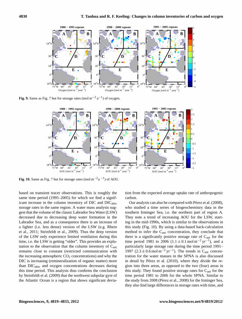
For oxygen and AOU a somewhat different picture emerges(Figs. 4 and 5). For the Atlantic Ocean as a whole there is anegative storage rate of oxygen; the average of all our datais −0.24 (CI:−0.41–(−0.07)) mol m−2 yr−1, and a positivestorage rate of AOU; 0.18 (CI: 0.004–0.32) mol m−2 yr−1.The storage rates of oxygen and AOU are significantly dif-ferent from zero for regions A and B only, as well for theaverage over all regions. Particularly, significant decrease inoxygen (and increase in AOU) column inventories are ob-served in the Labrador Sea, the Irminger Sea and in the north-

ern part of the Iceland Basin. The change in AOU, and theconfidence interval of the change, is somewhat smaller thanthat for oxygen indicting that some of variability is tied tochanges in solubility, mostly due to changes in temperatureof the water. This solubility component of the O2 changesmust be closely tied to the change in the inventory of heat.For instance, out-gassing of oxygen due to a warming oceanwill not cause any direct changes in AOU, i.e. changes inAOU are indicative of air-sea O2 fluxes driven by biology orcirculation. For the regions outside of SPNA, no significantchange in the column inventory of oxygen or AOU can bedetected with this method.

4.1 Temporal variations

In order to identify any temporal trends in storage rates,the data on storage rates for three different time periods areevaluated. Station pairs where both repeats are conductedin the any of the time-periods 1980–1995, 1990–2000, or1995–2005 were identified. This required discarding addi-tional pairs done more than 15 (or 10) yr apart, which furtherincreases the uncertainty of the storage rates for each area(i.e. decreases the number of available samples). Since theresulting coverage is very sparse in most regions, we focuson the two northernmost regions (A – the western part of theSPNA, and B – the eastern portion of the SPNA) where moredata is available, and where significant changes in deep wa-ter formation has occurred over time (e.g. Rhein et al., 2011).The data for the 3 time periods are displayed in Figs. 7 to 10for DIC, DICabio, oxygen and AOU, respectively. In Fig. 11the information for regions A and B is condensed.

It can be noted that, as expected, significant spatial vari-ations are present, even within each region, but that someinteresting patterns can be recognized. For the first time slice(1980–1995) an increase in oxygen, DIC and DICabio can beobserved for both regions (i.e. positive storage rates), partic-ular for region B, although only a limited number of stationpairs are available to confirm this trend. During the1990s theconditions are significantly different with negative storagerates of oxygen and close to neutral storage rates of DIC.During the last time slice (1995–2005) again a different pic-ture emerges with different patterns for the western and theeastern domain. For region A, the storage rate for oxygenis continuously negative whereas the DIC positive; region Bshow positive storage rates of DIC but neutral oxygen storagerates. It is clear that there are both temporal and spatial vari-ability in the storage rates of DIC and oxygen in the NorthAtlantic subpolar gyre, particularly for the northern part ofthe region.

5 Discussion

Based on estimates of the total storage of anthropogenic car-bon in the world ocean, the globally averaged storage rate for



−2

−1.5

−1

−0.5

0

0.5

1

1.5

2

2.5

3

DIC [mol m−2 year−1]

1995 − 2005 repeats

75oW 60o 45o 30o 15o 0o 18oS

0o

18o

36o

54oN

A B

C D

E


1990 − 2000 repeats

75oW 60o 45o 30o 15o 0o 18oS

0o

18o

36o

54oN

A B

C D

E


1980 − 1995 repeats

75oW 60o 45o 30o 15o 0o 18oS

0o

18o

36o

54oN

A B

C D

E

Fig. 7.Storage rates for DIC for three different time periods. Left panel – storage rates for repeats where both cruises were conducted between1980 and 1995; middle panel – both repeats were conducted between 1990 and 2000; right panel – both repeats were conducted between1995 and 2005. The 2000 m isobath is marked with a gray thin line.

DICabio


1990 − 2000 repeats

75oW 60o 45o 30o 15o 0o 18oS

0o

18o

36o

54oN

A B

C D

E

DICabio


1980 − 1995 repeats

75oW 60o 45o 30o 15o 0o 18oS

0o

18o

36o

54oN

A B

C D

E

−2

−1.5

−1

−0.5

0

0.5

1

1.5

2

2.5

3

DICabio


1995 − 2005 repeats

75oW 60o 45o 30o 15o 0o 18oS

0o

18o

36o

54oN

A B

C D

E

Fig. 8.Same as Fig. 7 but for storage rates (mol m−2 a−1) of DICabio.

Cant has been increasing from roughly 0.2 mol m−2 yr−1 in1960 to 0.6 mol m−2 yr−1 in 2007 (Khatiwala et al., 2009).The storage rate is expected to show significant regionalvariability assuming that the regional pattern of storage rateis similar to that of the total storage, see for instance theAtlantic Ocean map of Cant column inventory in Lee etal. (2003). However, there are a few important differencesbetween this study and the calculation by Lee et al. (2003).Most importantly this study reports on the change in DICand DICabio which is not equal to the change in Cant so thattemporal changes in the storage rate of DIC which is not evi-dent by observing the total storage of Cant becomes relevant.Changes in DICabio should be largely conserved in the oceaninterior as it compensates for respiration, but could changein surface water due to either air–sea exchange of CO2 orO2. Changes in column inventory of DICabio will thereforelargely reflect a combination of the effects of long-term CO2and O2 exchange with the atmosphere, with the CO2 effectpresumably dominating as a result of the uptake of anthro-

pogenic CO2. The regional patterns of storage rate of DICand DICabio in this analysis is significantly different than thewell-known distribution of column inventory of Cant in theAtlantic Ocean. In general, a mixed pattern of positive andnegative storage rates are found in each region. The picturegenerally gets somewhat less patchy when considering onlyshorter time-periods, Figs. 6–9. Since this method of calcu-lating storage rates does not account for small-scale temporaland spatial variability due to, for instance eddies and move-ments of oceanic fronts, larger variability in the storage rateis expected than from methods that do compensate for this,such as MLR based approaches. The larger scatter also reflectthe additional difficulties in determining inventory changesfor the total amount of DIC rather than the anthropogenicperturbation (Cant), see discussion below.

It is interesting to compare our result with the results pre-sented by Steinfedt et al. (2009) who observed only a weakincrease in the Cant column inventory (2 %) in the LabradorSea and Irminger Sea during the 1997–2003 time period



−5

−4

−3

−2

−1

0

1

2

3

4

5

Oxygen [mol m−2 year−1]

1995 − 2005 repeats

75oW 60o 45o 30o 15o 0o 18oS

0o

18o

36o

54oN

A B

C D

E


1990 − 2000 repeats

75oW 60o 45o 30o 15o 0o 18oS

0o

18o

36o

54oN

A B

C D

E


1980 − 1995 repeats

75oW 60o 45o 30o 15o 0o 18oS

0o

18o

36o

54oN

A B

C D

E

Fig. 9.Same as Fig. 7 but for storage rates (mol m−2 a−1) of oxygen.

AOU [mol m−2 year−1]

1980 − 1995 repeats

75oW 60o 45o 30o 15o 0o 18oS

0o

18o

36o

54oN

A B

C D

E


1990 − 2000 repeats

75oW 60o 45o 30o 15o 0o 18oS

0o

18o

36o

54oN

A B

C D

E

−3

−2.5

−2

−1.5

−1

−0.5

0

0.5

1

1.5

2

2.5

3


1995 − 2005 repeats

75oW 60o 45o 30o 15o 0o 18oS

0o

18o

36o

54oN

A B

C D

E

Fig. 10.Same as Fig. 7 but for storage rates (mol m−2a−1) of AOU.

based on transient tracer observations. This is roughly thesame time period (1995–2005) for which we find a signif-icant increase in the column inventory of DIC and DICabiostorage rates in the same region. A water mass analysis sug-gest that the volume of the classic Labrador Sea Water (LSW)decreased due to decreasing deep water formation in theLabrador Sea, and as a consequence there is an increase ofa lighter (i.e. less dense) version of the LSW (e.g. Rheinet al., 2011; Steinfeldt et al., 2009). Thus the deep versionof the LSW only experience limited ventilation during thistime, i.e. the LSW is getting “older”. This provides an expla-nation to the observation that the column inventory of Cantremains close to constant (restricted communication withthe increasing atmospheric CO2 concentrations) and why theDIC is increasing (remineralization of organic matter) morethan DICabio and oxygen concentrations decreases duringthis time period. This analysis thus confirms the conclusionby Steinfeldt et al. (2009) that the northwest subpolar gyre ofthe Atlantic Ocean is a region that shows significant devia-

tion from the expected average uptake rate of anthropogeniccarbon.

Our analysis can also be compared with Perez et al. (2008),who studied a time series of biogeochemistry data in thesouthern Irminger Sea, i.e. the northern part of region A.They note a trend of increasing AOU for the LSW, start-ing in the mid-1990s, which is similar to the observations inthis study (Fig. 10). By using a data-based back-calculationmethod to infer the Cant concentration, they conclude thatthere is a significantly positive storage rate of Cant for thetime period 1981 to 2006 (1.1± 0.1 mol m−2 yr−1), and aparticularly large storage rate during the time period 1991–1997 (2.3± 0.6 mol m−2 yr−1). The trends in Cant concen-tration for the water masses in the SPNA is also discussedin detail by Perez et al. (2010), where they divide the re-gion into three areas, as opposed to the two (four) areas inthis study. They found positive storage rates for Cant for thetime period 1981 to 2006 for the whole SPNA. Similar tothe study from 2008 (Perez et al., 2008) for the Irminger Sea,they also find large differences in storage rates with time, and



1980−1995 1990−2000 1995−2005−4

−3

−2

−1

0

1

2

3

4

stor

age

rate

[m

ol m

−2 y

−1 ]

Region A

DICDIC

abio

oxygen−AOU

1980−1995 1990−2000 1995−2005

Region B

DICDIC

abio

oxygen−AOU

Fig. 11. Storage rates for DIC, DICabio, AOU and oxygen for re-gions A and B for three time periods (1980–1995, 1990–2000, and1995–2005), see Figs. 6–9. Note that negative AOU is plotted andthat the markers are slightly offset for clarity. The error-bars the95 % confidence interval of the variation of storage rates within eacharea calculated from the values of the 2◦

× 2◦ bins (see text).

correlate this to the North Atlantic Oscillation (NAO) and theformation rate of Labrador Sea Water. They find particularlyhigh storage rates during the period 1991 to 1998 (i.e. duringthe time of intense formation of LSW) for the Irminger Seaand the Iceland Basin, whereas the East North Atlantic Basinseem to have a more linear increase of storage rate for Cant(0.77± 0.03 mol m−2 yr−1) (Perez et al., 2008, 2010). Thisoverlaps with the time period (1990–2000) where we findslightly negative storage rates for DIC and DICabio. However,since the analysis in this study is only covering the upper2000 m of the water column, storage changes in the deeperpart of the water column remains unaccounted for. For thisregion, with active deep water formation and significant ad-vection of overflow water, the deeper parts might indeed beimportant and is a source of error in this comparison. Signif-icant temporal variations inT , S and dissolved O2 occurredin the SPNA during the last∼ 60 yr are also reported by vanAken et al. (2011) who conclude that the long-term varia-tions of the intermediate water mass properties in the SPNAare related to meteorological forcing of the Labrador Sea.Significant changes in the SPNA salinity balance has beenobserved during the last half century (Curry and Mauritzen,2005) which can be consistent with varying dominance ofdifferent water masses. Based on this analysis it seems thatthese long-term variations also affect the inventory of DIC inthe SPNA.

The storage rates of DIC and DICabio in the southern partsof regions A and B are significantly higher than for the north-ern parts, and conform better to published estimates of Cantin the region. For instance, a recent study by McGrath etal. (2012) found storage rates of Cant in the Rockall Troughof 1.2 mol m−2 a−1 for the layer between 200 and 2000 m.The oxygen and AOU storage rates are close to neutral in thesouthern parts of regions A and B, i.e. similar to other areasfurther south in the Atlantic.

A detailed study of the temporal evolution of the inorganiccarbon content in the SPNA is out of scope for this study. Itis, however, interesting to point out the diverging trends ofCant and DIC found in this region may relate to varying con-vection activity and water mass distribution. It seems that theinventory of DIC decreases at the same time as the inven-tory of Cant increases. An explanation for this can be pro-vided by changes in water mass distribution in the SPNA.For instance, the DIC concentration of LSW is in the orderof 2160 µmol kg−1, whereas the DIC concentration of theMediterranean Sea Overflow Water (in the Gulf of Cadiz)is in the order of 2200 µmol kg−1, even though both watermasses have relatively high, and somewhat similar concen-tration of Cant. These two water masses are both present inthe SPNA and variability in the relative presence of thesetwo water masses will change the column inventory of DICin a way that is not necessarily reflected in storage of Cant.

Recently, Stendardo and Gruber (2012) used a long-termdata set for dissolved oxygen in the North Atlantic Ocean toassess any trends over the past 49 yr. She finds a complexpattern of temporal changes in oxygen concentrations; theupper water masses have generally lost oxygen, particularlyin the eastern and northern Atlantic, whereas deeper layershave generally gained oxygen, particularly in the southwest-ern part of the North Atlantic. The results are based on ob-served changes in oxygen concentration for different densityintervals (i.e. water masses). In a more detailed study focus-ing of repeats of the A2 sections (i.e. a zonal section acrossthe Atlantic Ocean at∼ 47◦ N), Stendardo (2011) concludesthat the oxygen concentrations show strong inter-annual vari-ability with a tendency towards oxygen loss over time. Theresults presented in this study are, in general, supporting theresults of Stendardo (2011) with particularly large losses ofoxygen in the northern part of the North Atlantic. However,the results are difficult to compare direct as this study is fo-cusing on the changes in column inventory rather than theconcentration in various water masses.

6 Concluding remarks

A simple method associated with few assumptions to con-strain the ocean storage rate of dissolved inorganic carbon(DIC), respiration corrected DIC (DICabio), oxygen, and ap-parent oxygen utilization (AOU) has been demonstrated. Bycalculating the difference in the column inventory of theseproperties down to 2000 m depth over the whole AtlanticOcean for a large number of repeat stations we find gen-erally find increase in DIC and a decrease of oxygen. Thetrends reported in this analysis supports other studies thathave reported on increasing concentrations of inorganic car-bon in the ocean based on more complicated schemes, andproviding some support for the general trend of ocean de-oxygenation. The degree of uncertainty in calculating trendsin interior ocean properties with this method demonstratesthe importance of small scale spatial and temporal variability



in the ocean. One important aspect of this analysis is thatvariations in water mass prevalence have a large influenceon inventories of interior ocean properties so that the totalDIC inventory can decrease in an area even if the inventoryof Cant significantly increases. This has implications for bal-ancing the global carbon budget that do not distinguish be-tween “anthropogenic carbon” and “natural carbon”. From aglobal perspective it is the overall increasing or decreasinginventory of carbon in the ocean that matters to balance thebudget.

Acknowledgements.The research leading to these results wassupported through EU FP7 project CARBOCHANGE “Changesin carbon uptake and emissions by oceans in a changing climate”which received funding from the European Community’s SeventhFramework Programme under grant agreement no. 264879. Wethank Mark Lenz for useful discussions on statistics. This work wascarried out in part while RFK was on sabbatical leave at the LeibnizInstitute of Marine Sciences in Kiel, supported by the HumboldtFoundation and the Cluster of Excellence “FutureOcean”.

Edited by: F. Joos

References

Anderson, L. A. and Sarmiento, J. L.: Redfield ratios of rem-ineralization determined by nutrient data analysis, Global Bio-geochem. Cy., 8, 65–80, 1994.

Cermeno, P., Dutkiewicz, S., Harris, R. P., Follows, M., Schofield,O., and Falkowski, P. G.: The role of nutricline depth in regulat-ing the ocean carbon cycle, P. Natl. Acad. Sci. USA, 105, 20344–20349,doi:10.1073/pnas.0811302106, 2008.

Curry, R. and Mauritzen, C.: Dilution of the Northern North At-lantic Ocean in Recent Decades, Science, 308, 1772–1774,doi:10.1126/science.1109477, 2005.

Friis, K., Kortzinger, A., Patsch, J., and Wallace, D. W. R.:On the temporal increase of anthropogenic CO2 in the sub-polar North Atlantic, Deep-Sea Res. Part I, 52, 681–698,doi:10.1016/j.dsr.2004.11.017, 2005.

Gammon, R. H., Cline, J., and Wisegarver, D. P.: Chluorofluo-romethanes in the Northeast Pacific Ocean: Measured Verti-cal Distribution and Application as Transient Tracers of UpperOcean Mixing, J. Geophys. Res., 87, 9441–9454, 1982.

Helm, K. P., Bindoff, N. L., and Church, J. A.: Observed decreasesin oxygen content of the global ocean, Geophys. Res. Lett., 38,L23602,doi:10.1029/2011gl049513, 2011.

Keeling, R. F.: Comment on “The Ocean Sink for AnthropogenicCO2”, Science, 308, 1743c, 2005.

Keeling, R. F. and Garcia, H. E.: The change in oceanic O-2 inven-tory associated with recent global warming, P. Natl. Acad. Sci.USA, 99, 7848–7853, 2002.

Keeling, R. F., Kortzinger, A., and Gruber, N.: Ocean Deoxygena-tion in a Warming World, Annual Review of Marine Science, 2,199–229,doi:10.1146/annurev.marine.010908.163855, 2010.

Key, R. M., Kozyr, A., Sabine, C. L., Lee, K., Wanninkhof, R.,Bullister, J. L., Feely, R. A., Millero, F. J., Mordy, C., and Peng,T. H.: A global ocean carbon climatology: Results from Global

Data Analysis Project (GLODAP), Global Biogeochem. Cy., 18,GB4031, doi:1029/2004GB002247, 2004.

Key, R. M., Tanhua, T., Olsen, A., Hoppema, M., Jutterstrom, S.,Schirnick, C., van Heuven, S., Kozyr, A., Lin, X., Velo, A., Wal-lace, D. W. R., and Mintrop, L.: The CARINA data synthesisproject: introduction and overview, Earth Syst. Sci. Data, 2, 105–121,doi:10.5194/essd-2-105-2010, 2010.

Khatiwala, S., Primeau, F., and Hall, T.: Reconstruction of the his-tory of anthropogenic CO2 concentrations in the ocean, Nature,462, 346–349,doi:10.1038/nature08526, 2009.

Kortzinger, A., Hedges, J. I., and Quay, P. D.: Redfield ratios revis-ited: Removing the biasing effect of anthropogenic CO2, Limnol.Oceanogr., 46, 964–970, 2001.

Lee, K., Choi, S.-D., Park, G.-H., Wanninkhof, R., Peng, T. H.,Key, R. M., Sabine, C. L., Feely, R. A., Bullister, J. L., Millero,F. J., and Kozyr, A.: An updated anthropogenic CO2 inven-tory in the Atlantic Ocean, Global Biogeochem. Cy., 17, 1116,doi:10.1029/2003GB002067, 2003.

Levine, N. M., Doney, S. C., Wanninkhof, R., Lindsay, K., andFung, I. Y.: Impact of ocean carbon system variability on the de-tection of temporal increases in anthropogenic CO2, J. Geophys.Res., 113, C03019,doi:10.1029/2007JC004153, 2008.

Levitus, S., Antonov, J. I., Boyer, T. P., Baranova, O. K., Garcia, H.E., Locarnini, R. A., Mishonov, A. V., Reagan, J. R., Seidov, D.,Yarosh, E. S., and Zweng, M. M.: World ocean heat content andthermosteric sea level change (0–2000 m), 1955–2010, Geophys.Res. Lett., 39, L10603,doi:10.1029/2012gl051106, 2012.

McGrath, T., Kivimae, C., Tanhua, T., Cave, R. R., and Mc-Govern, E.: Inorganic carbon and pH levels in the Rock-all Trough 1991–2010, Deep-Sea Res. Part I, 68, 79–91,doi:10.1016/j.dsr.2012.05.011, 2012.

Murata, A., Kumamoto, Y., Sasaki, K., Watanabe, S., and Fuka-sawa, M.: Decadal increases of anthropogenic CO2 in the sub-tropical South Atlantic Ocean along 30 degrees S, J. Geophys.Res., 113, C06007,doi:10.1029/2007JC004424, 2008.

Peng, T.-H. and Wanninkhof, R.: Increase in anthropogenic CO2 inthe Atlantic Ocean in the last two decades, Deep-Sea Res. Part I,57, 755–770,doi:10.1016/j.dsr.2010.03.008, 2010.

Perez, F. F., Vazquez-Rodrıguez, M., Louarn, E., Padın, X. A.,Mercier, H., and Rıos, A. F.: Temporal variability of the an-thropogenic CO2 storage in the Irminger Sea, Biogeosciences,5, 1669–1679,doi:10.5194/bg-5-1669-2008, 2008.

Perez, F. F., Vazquez-Rodrıguez, M., Mercier, H., Velo, A., Lher-minier, P., and Rıos, A. F.: Trends of anthropogenic CO2 storagein North Atlantic water masses, Biogeosciences, 7, 1789–1807,doi:10.5194/bg-7-1789-2010, 2010.

Pierrot, D., Brown, P., Van Heuven, S., Tanhua, T., Schuster,U., Wanninkhof, R., and Key, R. M.: CARINA TCO2 datain the Atlantic Ocean, Earth Syst. Sci. Data, 2, 177–187,doi:10.5194/essd-2-177-2010, 2010.

Rhein, M., Kieke, D., Huttl-Kabus, S., Roessler, A., Mertens, C.,Meissner, R., Klein, B., Boning, C. W., and Yashayaev, I.: Deepwater formation, the subpolar gyre, and the meridional overturn-ing circulation in the subpolar North Atlantic, Deep-Sea Res. PartII, 58, 1819–1832,doi:10.1016/j.dsr2.2010.10.061, 2011.

Riebesell, U., Schulz, K. G., Bellerby, R. G. J., Botros, M.,Fritsche, P., Meyerhofer, M., Neill, C., Nondal, G., Oschlies,A., Wohlers, J., and Zollner, E.: Enhanced biological carbonconsumption in a high CO2 ocean, Nature, 450, 545–548,


http://dx.doi.org/10.1073/pnas.0811302106

http://dx.doi.org/10.1126/science.1109477

http://dx.doi.org/10.1016/j.dsr.2004.11.017

http://dx.doi.org/10.1029/2011gl049513

http://dx.doi.org/10.1146/annurev.marine.010908.163855

http://dx.doi.org/10.5194/essd-2-105-2010

http://dx.doi.org/10.1038/nature08526

http://dx.doi.org/10.1029/2003GB002067

http://dx.doi.org/10.1029/2007JC004153

http://dx.doi.org/10.1029/2012gl051106


http://dx.doi.org/10.1029/2007JC004424


http://dx.doi.org/10.5194/bg-5-1669-2008

http://dx.doi.org/10.5194/bg-7-1789-2010


http://dx.doi.org/10.1016/j.dsr2.2010.10.061


doi:10.1038/nature06267, 2007.Rıos, A. F., Velo, A., Pardo, P. C., Hoppema, M., and Perez, F. F.:

An update of anthropogenic CO2 storage rates in the westernSouth Atlantic basin and the role of Antarctic Bottom Water, J.Mar. Systems, 94, 197–203,doi:10.1016/j.jmarsys.2011.11.023,2012.

Sabine, C. L. and Tanhua, T.: Estimation of Anthropogenic CO2Inventories in the Ocean, Annual Reviews of Marine Sciences,2, 175–198,doi:10.1146/annurev-marine-120308-080947, 2010.

Sabine, C. L., Key, R. M., Johnson, K. M., Millero, F. J., Pois-son, A., Sarmiento, J. L., Wallace, D. W. R., and Winn, C. D.:Anthropogenic CO2 inventory of the Indian Ocean, Global Bio-geochem. Cy., 13, 179–198, 1999.

Sabine, C. L., Key, R. M., Kozyr, A., Feely, R. A., Wanninkhof,R., Millero, F., Peng, T. H., Bullister, J., and Lee, K.: GlobalOcean data analysis project (GLODAP): Results and data,ORNL/CDIAC-145, NDP-083, 2005.

Schneider, A., Tanhua, T., Kortzinger, A., and Wallace, D. W.R.: An evaluation of tracer fields and anthropogenic car-bon in the equatorial and the tropical North Atlantic, Deep-Sea Res. Part I: Oceanographic Research Papers, 67, 85–97,doi:10.1016/j.dsr.2012.05.007, 2012.

Steinfeldt, R., Rhein, M., Bullister, J. L., and Tanhua, T.: Inven-tory changes in anthropogenic carbon from 1997–2003 in the At-lantic Ocean between 20 degrees S and 65 degrees N, Global Bio-geochem. Cy., 23, GB3010,doi:10.1029/2008GB003311, 2009.

Stendardo, I.: Interannual to decadal variability and trends of theoceanic oxygen content in the North Atlantic, PhD, Institute ofBiogeochemistry and Pollutant Dynamics, ETH, Zurich, 185 pp.,2011.

Stendardo, I., and Gruber, N.: Oxygen trends over five decadesin the North Atlantic, J. Geophys. Res., 117, C11004,doi:10.1029/2012jc007909, 2012.

Stendardo, I., Gruber, N., and Kortzinger, A.: CARINA oxygendata in the Atlantic Ocean, Earth Syst. Sci. Data, 1, 87–100,doi:10.5194/essd-1-87-2009, 2009.

Tanhua, T. and Wallace, D. W. R.: Consistency of TTO-NAS Inor-ganic Carbon Data with modern measurements, Geophys. Res.Lett., 32, L14618,doi:10.1029/2005GL023248, 2005.

Tanhua, T., Kortzinger, A., Friis, K., Waugh, D. W., and Wallace, D.W. R.: An estimate of anthropogenic CO2 inventory from decadalchanges in ocean carbon content, P. Natl. Acad. Sci. USA., 104,3037–3042,doi:10.1073/pnas.0606574104, 2007.

Tanhua, T., van Heuven, S., Key, R. M., Velo, A., Olsen, A.,and Schirnick, C.: Quality control procedures and methodsof the CARINA database, Earth Syst. Sci. Data, 2, 35–49,doi:10.5194/essd-2-35-2010, 2010.

Touratier, F. and Goyet, C.: Decadal evolution of anthropogenicCO2 in the northwestern Mediterranean Sea from the mid-1990s to the mid-2000s, Deep-Sea Res. Part I, 56, 1708–1716,doi:10.1016/j.dsr.2009.05.015, 2009.

Touratier, F., Azouzi, L., and Goyet, C.: CFC-11, Delta C-14 and H-3 tracers as a means to assess anthropogenic CO2 concentrationsin the ocean, Tellus B, 59, 318–325, 2007.

van Aken, H. M., Femke de Jong, M., and Yashayaev, I.: Decadaland multi-decadal variability of Labrador Sea Water in the north-western North Atlantic Ocean derived from tracer distributions:Heat budget, ventilation, and advection, Deep-Sea Res. Part I,58, 505–523,doi:10.1016/j.dsr.2011.02.008, 2011.

Velo, A., Perez, F. F., Brown, P., Tanhua, T., Schuster, U., and Key,R. M.: CARINA alkalinity data in the Atlantic Ocean, Earth Syst.Sci. Data, 1, 45–61,doi:10.5194/essd-1-45-2009, 2009.

Wakita, M., Watanabe, S., Murata, A., Tsurushima, N., and Honda,M.: Decadal change of dissolved inorganic carbon in the sub-arctic western North Pacific Ocean, Tellus B, 62, 608–620,doi:10.1111/j.1600-0889.2010.00476.x, 2010.

Wanninkhof, R., Doney, S. C., Bullister, J. L., Levine, N. M.,Warner, M., and Gruber, N.: Detecting anthropogenic CO2changes in the interior Atlantic Ocean between 1989 and 2005, J.Geophys. Res., 115, C11028,doi:10.1029/2010JC006251, 2010.

Weiss, R.: Solubility of Nitrogen, Oxygen and Argon in water andseawater, Deep-Sea Res., 17, 721–735, 1970.

Yool, A., Oschlies, A., Nurser, A. J. G., and Gruber, N.: A model-based assessment of the TrOCA approach for estimating an-thropogenic carbon in the ocean, Biogeosciences, 7, 723–751,doi:10.5194/bg-7-723-2010, 2010.


http://dx.doi.org/10.1038/nature06267

http://dx.doi.org/10.1016/j.jmarsys.2011.11.023

http://dx.doi.org/10.1146/annurev-marine-120308-080947


http://dx.doi.org/10.1029/2008GB003311

http://dx.doi.org/10.1029/2012jc007909


http://dx.doi.org/10.1029/2005GL023248

http://dx.doi.org/10.1073/pnas.0606574104





http://dx.doi.org/10.1111/j.1600-0889.2010.00476.x

http://dx.doi.org/10.1029/2010JC006251

http://dx.doi.org/10.5194/bg-7-723-2010

changes in column inventories of carbon and oxygen in the atlantic

Documents