Chalmers Publication Library

On the Required Number of Antennas in a Point-to-Point Large-but-Finite MIMOSystem: Outage-Limited Scenario

This document has been downloaded from Chalmers Publication Library (CPL). It is the author´s

version of a work that was accepted for publication in:

IEEE Transactions on Communications (ISSN: 0090-6778)

Citation for the published paper:Makki, B. ; Svensson, T. ; Eriksson, T. et al. (2016) "On the Required Number of Antennasin a Point-to-Point Large-but-Finite MIMO System: Outage-Limited Scenario". IEEETransactions on Communications

Downloaded from: http://publications.lib.chalmers.se/publication/234013

Notice: Changes introduced as a result of publishing processes such as copy-editing and

formatting may not be reflected in this document. For a definitive version of this work, please refer

to the published source. Please note that access to the published version might require a

subscription.

Chalmers Publication Library (CPL) offers the possibility of retrieving research publications produced at ChalmersUniversity of Technology. It covers all types of publications: articles, dissertations, licentiate theses, masters theses,conference papers, reports etc. Since 2006 it is the official tool for Chalmers official publication statistics. To ensure thatChalmers research results are disseminated as widely as possible, an Open Access Policy has been adopted.The CPL service is administrated and maintained by Chalmers Library.

(article starts on next page)

1

On the Required Number of Antennas in aPoint-to-Point Large-but-Finite MIMO System:

Outage-Limited ScenarioBehrooz Makki, Tommy Svensson, Thomas Eriksson and Mohamed-Slim Alouini, Fellow, IEEE

Abstract—This paper investigates the performance of the point-to-point multiple-input-multiple-output (MIMO) systems in thepresence of a large but finite numbers of antennas at the trans-mitters and/or receivers. Considering the cases with and withouthybrid automatic repeat request (HARQ) feedback, we determinethe minimum numbers of the transmit/receive antennas whicharerequired to satisfy different outage probability constraints. Ourresults are obtained for different fading conditions and the effectof the power amplifiers efficiency/feedback error probability onthe performance of the MIMO-HARQ systems is analyzed. Then,we use some recent results on the achievable rates of finite block-length codes, to analyze the effect of the codewords lengthson the system performance. Moreover, we derive closed-formexpressions for the asymptotic performance of the MIMO-HARQsystems when the number of antennas increases. Our analyticaland numerical results show that different outage requirementscan be satisfied with relatively few transmit/receive antennas.

I. I NTRODUCTION

The next generation of wireless networks must provide datastreams for everyone everywhere at any time. Particularly,the data rates should be orders of magnitude higher thanthose in the current systems; a demand that creates seriouspower concerns because the data rate scales with power mono-tonically. The problem becomes even more important whenwe remember that currently the wireless network contributes∼ 2% of global CO2 emissions and its energy consumption isexpected to increase16− 20% every year [1].

To address the demands, the main strategy persuaded inthe last few years is the networkdensification[2]. One ofthe promising techniques to densify the network is to usemany antennas at the transmit and/or receive terminals. Thisapproach is referred to as massive or large multiple-input-multiple-output (MIMO) in the literature.

In general, the more antennas the transmitter and/or thereceiver are equipped with, the better the data rate/link re-liability. Particularly, the capacity increases and the requireduplink/downlink transmit power decreases with the numberof antennas. Thus, the trend is towards asymptotically highnumber of antennas. This is specially because millimeter wave

Behrooz Makki, Tommy Svensson and Thomas Eriksson are with ChalmersUniversity of Technology, Gothenburg, Sweden, Email:behrooz.makki,tommy.svensson, thomase@chalmers.se. Mohamed-Slim Alouini is with theKing Abdullah University of Science and Technology (KAUST), Thuwal,Makkah Province, Saudi Arabia, Email: slim.alouini@kaust.edu.sa

Part of this work has been accepted for presentation at the IEEE ICUWB2015.

The research leading to these results received funding fromthe EuropeanCommission H2020 programme under grant agreementn671650 (5G PPPmmMAGIC project), and from the Swedish Governmental Agencyfor Inno-vation Systems (VINNOVA) within the VINN Excellence CenterChase.

communication [3], [4], which is indeed expected to be im-plemented in the next generation of wireless networks, makesit possible to assemble many antennas at the transmit/receiveterminals. However, large MIMO implies challenges such ashardware impairments and signal processing complexity whichmay limit the number of antennas in practice. Also, one ofthe main bottlenecks of large MIMO is the channel stateinformation (CSI) acquisition, specifically at the transmitter.Therefore, it is interesting to use efficient feedback schemessuch as hybrid automatic repeat request (HARQ) whose feed-back overhead does not scale with the number of antennas.

The performance of HARQ protocols in single-input-single-output (SISO) and MIMO systems is studied in, e.g., [5]–[8] and [9]–[20], respectively. MIMO transmission with manyantennas is advocated in [21], [22] where the time-divisionduplex (TDD)-based training is utilized for CSI feedback1.Also, [23]–[29] introduce TDD-based schemes for large sys-tems. Particularly, [29] studies the required number of antennasin TDD-based multi-cellular systems with pilot contaminationbeing the major issue. Here, different precoders are designedsuch that the network sum throughput is optimized. In themeantime, frequency division duplex (FDD)-based massiveMIMO has recently attracted attentions and low-overhead CSIacquisition methods were proposed [30]–[32]. Consideringim-perfect CSI, [33] derives lower bounds for the uplink achiev-able rate of the MIMO setups with large but finite number ofantennas. Then, [34] (resp. [35]) studies the zero-forcingbasedTDD (resp. TDD/FDD) systems under the assumption thatthe number of transmit antennas and the single-antenna usersare asymptotically large while their ratio remains bounded.Finally, [39] derives approximate expressions for the mutualinformation of MIMO systems with large number of transmitand/or receive antennas, and evaluates the effect of quantizedfeedback/scheduling on the system performance (For detailedreview of the literature on massive MIMO, see [36]–[38]).

To summarize, a large part of the literature on the point-to-point and multi-user large MIMO is based on the assumptionof asymptotically many antennas. Then, a natural questionis how many transmit/receive antennas do we require inpractice to satisfy different quality-of-service requirements.The interesting answer this paper establishes is relatively few,for a large range of outage probabilities. Moreover, the results

1The results of [21]–[38] are mostly on multi-user MIMO networks, asopposed to our work on point-to-point systems. However, because many ofthe analytical results in [21]–[38] are applicable in point-to-point systems aswell, these works are cited.

2

of [5]–[39] are mainly obtained under the assumption that theinstantaneous achievable rate of a user is given bylog(1 + x)with x standing for the user’s instantaneous received signal-to-interference-and-noise ratio (SINR). This is an appropriateassumption in the cases with long codewords. However, it isalso interesting to analyze the system performance in the caseswith codewords of finite length wherelog(1 + x) is not anappropriate approximation for the achievable rates.

Here, we study the outage-limited performance of point-to-point MIMO systems in the cases with large but finitenumber of antennas. Using the fundamental results of [39] onthe mutual information of MIMO setups, we derive closed-form expressions for the required number of transmit and/orreceive antennas satisfying various outage probability require-ments (Theorem 1). The results are obtained for differentfading conditions and in the cases with or without HARQ.Furthermore, we analyze the effect of the power amplifiers(PAs) efficiency (Section IV.A), erroneous feedback (SectionIV.C) and spatial/temporal correlations (Sections V.B, V.C) onthe system performance and study the outage probability inthe cases with adaptive power allocation between the HARQretransmissions (Theorem 3). Then, we use the recent resultsof [40], [41] on the achievable rates of finite block-lengthcodes to analyze the outage probability in the cases withshort packets and erroneous feedback (Section IV.C). Finally,we study the asymptotic performance of MIMO systems.Particularly, denoting the outage probability and the numberof transmit and receive antennas byPr(Outage), Nt andNr,

respectively, we derive closed-form expressions for the nor-malized outage factor which is defined asΓ = − log(Pr(Outage))

NtNr

when the number of transmit and/or receive antennas increases(Theorem 2).

As opposed to [5]–[20], we consider large MIMO setupsand determine the required number of antennas in outage-limited conditions. Also, the paper is different from [21]–[39]because we study the outage-limited scenarios in point-to-point systems, implement HARQ and the number of antennasis considered to be finite. The differences in the problemformulation and the channel model makes the problem solvedin this paper completely different from the ones in [5]–[39], leading to different analytical/numerical results,as wellas to different conclusions. Finally, our discussions on theasymptotic outage performance of the MIMO setups, finiteblock-length analysis and the effect of PAs on the performanceof MIMO-HARQ schemes have not been presented before.

Our analytical and numerical results indicate that:• Different quality-of-service requirements can be satisfied

with relatively few transmit/receive antennas. For in-stance, consider a SIMO (S: single) setup without HARQand transmission signal-to-noise ratio (SNR)5 dB. Then,with the data rate of 3 nats-per-channel use (npcu), theoutage probabilities10−3, 10−4 and10−5 are guaranteedwith 16, 18 and 20 receive antennas, respectively (Fig.5a). Also, the implementation of HARQ reduces therequired number of antennas significantly (Fig. 3).

• At moderate/high SNRs, the required number of transmit(resp. receive) antennas scales with(Q−1(θ))2, 1

MT, and

1(log(φ))2 linearly, if the number of receive (resp. transmit)

antennas is fixed. Here,M is the maximum numberof HARQ retransmission rounds,T is the number ofchannel realizations experienced in each round,φ denotesthe SNR, θ is the outage probability constraint andQ−1(.) represents the inverse GaussianQ-function. Thesescaling laws are changed drastically, if the numbers of thetransmit and receive antennas are adapted simultaneously(see Theorem 1 and its following discussions for details).

• For different fading conditions, the normalized outagefactorΓ = − log(Pr(Outage))

NtNrconverges to constant values,

unless the number of receive antennas grows large whilethe number of transmit antennas is fixed (see Theorem2). Also, for every given number of transmit/receiveantennas, the normalized outage factor increases withMT linearly.

• There are mappings between the performance of MIMO-HARQ systems in quasi-static, slow- and fast-fadingconditions, in the sense that with proper scaling ofthe channel parameters the same outage probability isachieved in these conditions. This point provides anappropriate connection between the papers consideringone of these fading models.

• Adaptive power allocation between the HARQ retrans-missions leads to marginal antenna requirement reduc-tion, while the system performance is remarkably affectedby the inefficiency of the PAs. Also, the spatial correlationbetween the antennas increases the required number ofantennas while, for a large range of correlation condi-tions, the same scaling rules hold for the uncorrelatedand correlated fading scenarios.

• Finally, with low number of antennas the system per-formance is considerably affected by the feedback errorprobability. However, the effect of erroneous feedbackdecreases with the number of antennas. Moreover, fora given number of nats per codeword, increasing thenumber of antennas can effectively reduce the requiredcodeword length leading to low data transmission delay.

Notations. In the following, we denote the determinant,the Hermitian and the(i, j)-th element of the matrixXby |X|, Xh and X[i, j], respectively. Also,E[·] is the ex-pectation operator,

⊗

denotes the Kronecker product and

Q(x) = 1√2π

∫∞x

e−u2

2 du is the GaussianQ-function. Then,⌈x⌉ denotes the smallest integer number larger than or equalto x, and thearg function is used to indicate the solution ofan equation. Finally,Q−1(·) andW (·) represent the inverseQ-function and the Lambert W function, respectively.

II. SYSTEM MODEL

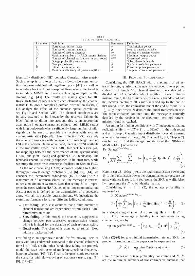
Table 1 summarizes the set of parameters used throughoutthe paper. We consider a point-to-point MIMO setup withNt transmit antennas andNr receive antennas. We study theblock-fading conditions where the channel coefficients remainconstant during the channel coherence time and then change toother values based on their probability density function (PDF).In this way, the received signal is given by

Y = HX + Z,Z ∈ CNr×1, (1)

where H ∈ CNr×Nt is the fading matrix,X ∈ CNt×1 is thetransmitted signal andZ ∈ CNr×1 denotes the independent and

3

Table ITHE DEFINITION OF PARAMETERS.

Parameter Definition Parameter DefinitionΓ Normalized outage factor φ Transmission powerNt Number of transmit antennas µ Mean of a random variableNr Number of receive antennas σ2 Variance of a random variableM Maximum number of HARQ retransmissions φmax Maximum output powerT Number of channel realizations in each roundφcons Consumed powerθ Outage probability constraint L Sub-codewords lengthq Nats per codeword β Spatial correlation parameterR Initial transmission rate ϑ Power amplifier parameterǫ Maximum efficiency of power amplifier ν Temporal correlation parameter

identically distributed (IID) complex Gaussian noise matrix.Such a setup is of interest in, e.g., side-to-side communica-tion between vehicles/buildings/lamp posts [42], as well asin wireless backhaul point-to-point links where the trend isto introduce MIMO and thereby achieving multiple parallelstreams, e.g., [43]. The results are mainly given for IIDRayleigh-fading channels where each element of the channelmatrix H follows a complex Gaussian distributionCN (0, 1)(To analyze the effect of the antennas spatial correlation,see Fig. 9 and Section V.B). The channel coefficients areinitially assumed to be known by the receiver. Taking theblock-fading condition into account, this is an appropriateassumption in outage-constrained point-to-point MIMO setupswith long codewords where sufficiently large number of pilotsignals can be used to provide the receiver with accuratechannel estimation [5]–[20]. Then, in Section IV.C, we studythe other extreme case with codewords of finite length and noCSI at the receiver. On the other hand, there is no CSI availableat the transmitter except the HARQ feedback bits (see [44]for mappings between the performance of the systems usingHARQ and joint HARQ and quantized CSI feedback). Thefeedback channel is initially supposed to be error-free, whilewe study the cases with erroneous feedback in Section IV.C.

As the most promising HARQ approach leading to highestthroughput/lowest outage probability [5], [6], [9], [14],weconsider the incremental redundancy (INR) HARQ with amaximum ofM retransmissions, i.e., the message is retrans-mitted a maximum ofM times. Note that settingM = 1 repre-sents the cases without HARQ, i.e., open-loop communication.Also, a packet is defined as the transmission of a codewordalong with all its possible retransmissions. We investigate thesystem performance for three different fading conditions:

• Fast-fading. Here, it is assumed that a finite number ofchannel realizations are experienced within each HARQretransmission round.

• Slow-fading. In this model, the channel is supposed tochange between two successive retransmission rounds,while it is fixed for the duration of each retransmission.

• Quasi-static. The channel is assumed to remain fixedwithin a packet period.

Fast-fading is an appropriate model for fast-moving users orusers with long codewords compared to the channel coherencetime [14], [45]. On the other hand, slow-fading can properlymodel the cases with users of moderate speeds or frequency-hopping schemes [10]–[12]. Finally, the quasi-static representsthe scenarios with slow-moving or stationary users, e.g., [5],[9], [17]–[20].

III. PROBLEM FORMULATION

Considering the INR HARQ with a maximum ofM re-transmissions,q information nats are encoded into aparentcodeword of lengthML channel uses and the codeword isdivided intoM sub-codewords of lengthL. In each retrans-mission round, the transmitter sends a new sub-codeword andthe receiver combines all signals received up to the end ofthat round. Thus, the equivalent rate at the end of roundm isq

mL= R

mnpcu whereR denotes the initial transmission rate.

The retransmissions continue until the message is correctlydecoded by the receiver or the maximum permitted retrans-mission round is reached.

Assuming fast-fading conditions withT independent fadingrealizationsH((m− 1)T + 1), . . . , H(mT ) in themth roundand an isotropic Gaussian input distribution over all transmitantennas, the results of, e.g., [46, Chapter 15], [47, Chapter 7],can be used to find the outage probability of the INR-basedMIMO-HARQ scheme asPr(Outage)Fast-fading=

Pr

1

MT

M∑

n=1

nT∑

t=(n−1)T+1

log

∣

∣

∣

∣

INr +φ

NtH(t)H(t)h

∣

∣

∣

∣

≤ R

M

.

(2)

Here,φ (in dB, 10 log10 φ) is the total transmission power andφNt

is the transmission power per transmit antenna (because thenoise variance is set to 1,φ represents the SNR as well). Also,INr represents theNr ×Nr identity matrix.

ConsideringT = 1 in (2), the outage probability isrephrased as

Pr(Outage)Slow-fading=

Pr

(

1

M

M∑

n=1

log

∣

∣

∣

∣

INr +φ

NtH(n)H(n)h

∣

∣

∣

∣

≤ R

M

)

, (3)

in a slow-fading channel. Also, settingH(t) = H, ∀t =1, . . . ,MT, the outage probability in a quasi-static fadingchannel is given by

Pr(Outage)Quasi-static= Pr

(

log

∣

∣

∣

∣

INr +φ

NtHHh

∣

∣

∣

∣

≤ R

M

)

.

(4)

Using (2)-(4) for given initial transmission rate and SNR, theproblem formulation of the paper can be expressed as

Nt, Nr = argminNt,Nr

Pr(Outage) ≤ θ. (5)

Here, θ denotes an outage probability constraint andNt, Nr

are the minimum numbers of transmit/receive antennas that

4

are required to satisfy the outage probability constraint.In thefollowing, we solve (5) in the cases where one of the transmitor receive antennas is given, or there is a relationship betweenthe number of transmit and receive antennas. Particularly,westudy (5) in four distinct cases:

• Case 1:Nr is large butNt is given.• Case 2:Nr is given butNt is large.• Case 3: BothNt andNr are large and the transmission

SNR is low.• Case 4: BothNt andNr are large and the transmission

SNR is high.It is worth noting that the three first cases are commonly ofinterest in large MIMO systems. However, for the complete-ness of the discussions, we consider Case 4 as well. Moreover,in harmony with the literature [34], [35]2, we analyze Cases3-4 under the assumption

Nt

Nr= K, (6)

with K being a constant. However, as seen in the following,it is straightforward to extend the results of the paper to thecases with other relations between the numbers of antennas.

The basis of our analyses comes from the well-establishedresults of [39] which approximate the instantaneous mutualinformation of MIMO setups by equivalent Gaussian variables.Then, we use the results to derive the minimum numberof transmit/receive antennas in outage-constrained conditions(Theorem 1), define and analyze the normalized outage factor(Theorem 2), study the effect of imperfect power amplifiers(Section IV.A), derive outage-optimized power allocationbe-tween the HARQ retransmissions (Theorem 3), and performfinite block-length analysis of MIMO-HARQ systems witherroneous feedback (Section IV.C).

Finally, we should mention that, as (5) is a non-convexproblem, there is no guarantee that the globally optimalparameters are determined by any method, except exhaustivesearch algorithms. However, as we show in Section V, ourapproximation schemes lead to very close results to the onesobtained by exhaustive search.

IV. PERFORMANCEANALYSIS

To solve (5), let us first introduce Lemma 1. The lemmais of interest because it represents the outage probabilityasa function of the number of antennas, and simplifies theperformance analysis remarkably.

Lemma 1: Considering Cases 1-4, the outage probability ofthe INR-based MIMO-HARQ system is given by

Pr(Outage)Fast-fading= Q(√

MT (µ− RM

)

σ

)

, (i)

Pr(Outage)Slow-fading= Q(√

M(µ− RM

)

σ

)

, (ii)

Pr(Outage)Quasi-static= Q(

µ− RM

σ

)

, (iii)

(7)

where for different casesµ andσ are given in (8).Proof. The proof is based on (2)-(4) and [39, Theorems 1-

3], where considering Cases 1-4 the random variableZ(t) =log |INr+

φNt

H(t)H(t)h| converges in distribution to a Gaussian

2In [34], [35], which study multi-user MIMO setups,Nt and Nr aresupposed to follow (6) while, as opposed to our work, they areconsidered tobe asymptotically large.

random variableY ∼ N (µ, σ2) which, depending on thenumbers of antennas, has the following characteristics

(µ, σ2) =

(

Nt log(

1 + NrφNt

)

, NtNr

)

, if Case 1(

Nr log (1 + φ) , Nrφ2

Nt(1+φ)2

)

, if Case 2(

Nrφ,NrNtφ2)

, if Case 3(

µ, σ2)

, if Case 4

µ = Nmin log

(

φ

Nt

)

+Nmin

(

Nmax−Nmin∑

i=1

1

i− γ

)

+

Nmin−1∑

i=1

i

Nmax− i, γ = 0.5772 . . .

σ2 =

Nmin−1∑

i=1

i

(Nmax−Nmin + i)2+Nmin

(

π2

6−

Nmax−1∑

i=1

1

i2

)

,

Nmax.= max(Nt, Nr), Nmin

.= min(Nt, Nr). (8)

In this way, from (2) and for different cases, the outageprobability in fast-fading condition is given by

Pr(Outage)Fast-fading= Pr

(

Z ≤ R

M

)

, Z.=

1

MT

MT∑

t=1

Z(t),

(9)

where, becauseZ is the average ofMT independent Gaus-sian random variablesY ∼ N (µ, σ2), we have Z ∼N (µ, 1

MTσ2). Consequently, using the cumulative distribution

function (CDF) of Gaussian random variables, the outageprobability in fast-fading condition is given by (7.i). Thesamearguments can be applied to derive (7.ii-iii) in slow-fading andquasi-static conditions.

The advantage of Lemma 1 is that, as seen in the follow-ing, it replaces the complicated optimization problem (5) byfinding the solution of very simple equations with no need forderivatives or other optimization techniques. Then, as we showin Section V, in all cases the derived analytical results matchwith the ones found via simulations with very high accuracy.Moreover, Lemma 1 leads to the following corollaries:

1) For Cases 1-4, using INR MIMO-HARQ in the quasi-static, slow- and fast-fading channels leads to scalingthe variance of the equivalent random variable by1, MandMT , respectively. That is, using HARQ, there existsmappings between the quasi-static, the slow- and the fast-fading conditions in the sense that with proper scaling ofσ in (7) they lead to the same outage probability.

2) With asymptotically large numbers of transmit and/orreceive antennas, the optimal data rate which leads tozero outage probability and maximum throughput is givenby R = µ − ω, ω → 0, with µ derived in (8); Interest-ingly, the result is independent of the fading condition.Also, with asymptotically high number of antennas andR = µ − ω, ω → 0, no HARQ is needed because themessage is decoded in the first round (with probability1).

3) Finally, using (7), we can map the MIMO-HARQ sys-tem into an equivalent SISO-HARQ setup whose fadingfollows N (µ, σ2) with µ andσ given in (8) for differentcases.

5

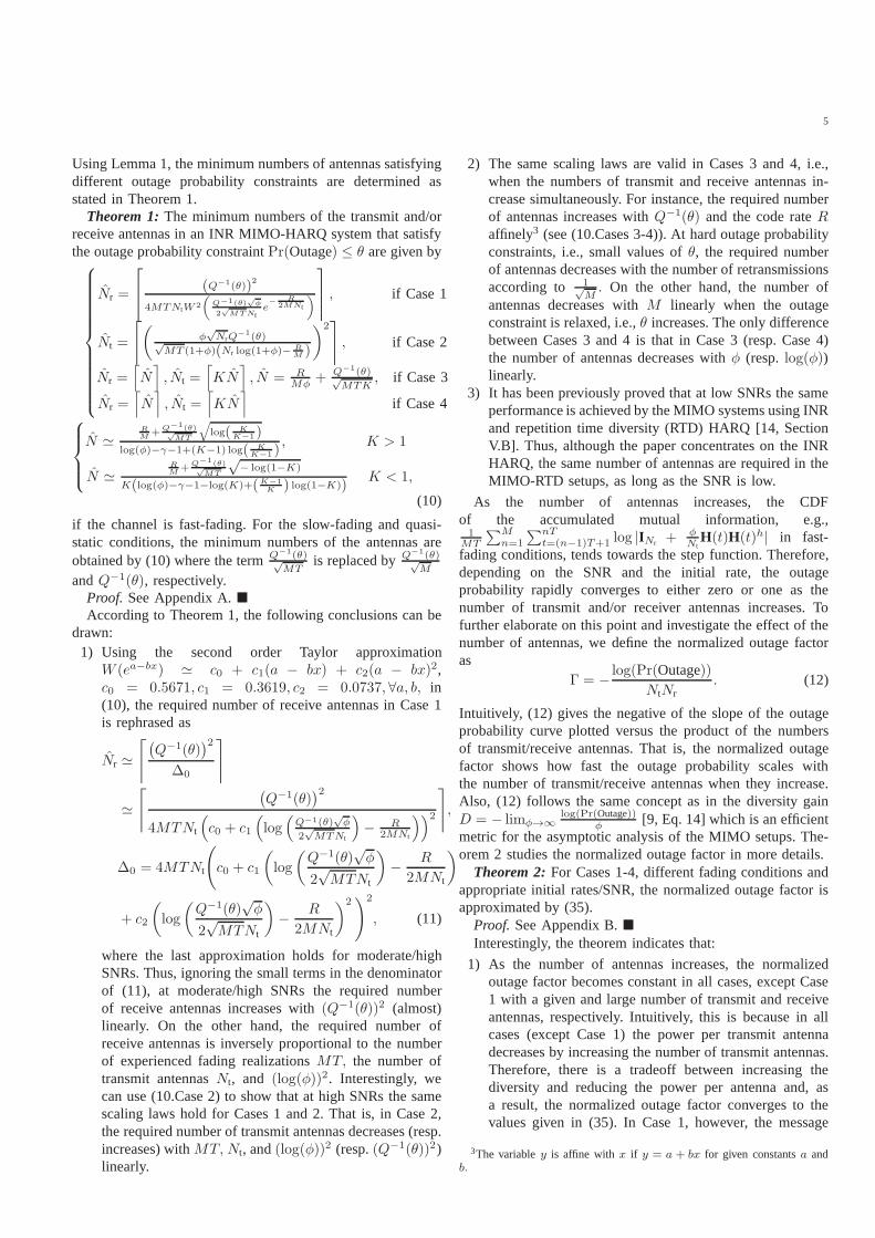
Using Lemma 1, the minimum numbers of antennas satisfyingdifferent outage probability constraints are determined asstated in Theorem 1.

Theorem 1: The minimum numbers of the transmit and/orreceive antennas in an INR MIMO-HARQ system that satisfythe outage probability constraintPr(Outage) ≤ θ are given by

Nr =

(Q−1(θ))2

4MTNtW 2

(

Q−1(θ)√

φ

2√

MTNte−

R2MNt

)

, if Case 1

Nt =

⌈

(

φ√NrQ

−1(θ)√MT (1+φ)(Nr log(1+φ)− R

M )

)2⌉

, if Case 2

Nr =⌈

N⌉

, Nt =⌈

KN⌉

, N = RMφ

+ Q−1(θ)√MTK

, if Case 3

Nr =⌈

N⌉

, Nt =⌈

KN⌉

if Case 4

N ≃RM

+Q−1(θ)√

MT

√

log( KK−1 )

log(φ)−γ−1+(K−1) log( KK−1 )

, K > 1

N ≃RM

+Q−1(θ)√

MT

√− log(1−K)

K(log(φ)−γ−1−log(K)+(K−1K ) log(1−K))

K < 1,

(10)

if the channel is fast-fading. For the slow-fading and quasi-static conditions, the minimum numbers of the antennas areobtained by (10) where the termQ

−1(θ)√MT

is replaced byQ−1(θ)√M

andQ−1(θ), respectively.Proof. See Appendix A.According to Theorem 1, the following conclusions can be

drawn:1) Using the second order Taylor approximation

W (ea−bx) ≃ c0 + c1(a − bx) + c2(a − bx)2,c0 = 0.5671, c1 = 0.3619, c2 = 0.0737, ∀a, b, in(10), the required number of receive antennas in Case 1is rephrased as

Nr ≃⌈

(

Q−1(θ))2

∆0

⌉

≃⌈

(

Q−1(θ))2

4MTNt

(

c0 + c1

(

log(

Q−1(θ)√φ

2√MTNt

)

− R2MNt

))2

⌉

,

∆0 = 4MTNt

(

c0 + c1

(

log

(

Q−1(θ)√φ

2√MTNt

)

− R

2MNt

)

+ c2

(

log

(

Q−1(θ)√φ

2√MTNt

)

− R

2MNt

)2)2

, (11)

where the last approximation holds for moderate/highSNRs. Thus, ignoring the small terms in the denominatorof (11), at moderate/high SNRs the required numberof receive antennas increases with(Q−1(θ))2 (almost)linearly. On the other hand, the required number ofreceive antennas is inversely proportional to the numberof experienced fading realizationsMT, the number oftransmit antennasNt, and (log(φ))2. Interestingly, wecan use (10.Case 2) to show that at high SNRs the samescaling laws hold for Cases 1 and 2. That is, in Case 2,the required number of transmit antennas decreases (resp.increases) withMT, Nt, and(log(φ))2 (resp.(Q−1(θ))2)linearly.

2) The same scaling laws are valid in Cases 3 and 4, i.e.,when the numbers of transmit and receive antennas in-crease simultaneously. For instance, the required numberof antennas increases withQ−1(θ) and the code rateRaffinely3 (see (10.Cases 3-4)). At hard outage probabilityconstraints, i.e., small values ofθ, the required numberof antennas decreases with the number of retransmissionsaccording to 1√

M. On the other hand, the number of

antennas decreases withM linearly when the outageconstraint is relaxed, i.e.,θ increases. The only differencebetween Cases 3 and 4 is that in Case 3 (resp. Case 4)the number of antennas decreases withφ (resp.log(φ))linearly.

3) It has been previously proved that at low SNRs the sameperformance is achieved by the MIMO systems using INRand repetition time diversity (RTD) HARQ [14, SectionV.B]. Thus, although the paper concentrates on the INRHARQ, the same number of antennas are required in theMIMO-RTD setups, as long as the SNR is low.

As the number of antennas increases, the CDFof the accumulated mutual information, e.g.,1

MT

∑Mn=1

∑nTt=(n−1)T+1 log |INr + φ

NtH(t)H(t)h| in fast-

fading conditions, tends towards the step function. Therefore,depending on the SNR and the initial rate, the outageprobability rapidly converges to either zero or one as thenumber of transmit and/or receiver antennas increases. Tofurther elaborate on this point and investigate the effect of thenumber of antennas, we define the normalized outage factoras

Γ = − log(Pr(Outage))NtNr

. (12)

Intuitively, (12) gives the negative of the slope of the outageprobability curve plotted versus the product of the numbersof transmit/receive antennas. That is, the normalized outagefactor shows how fast the outage probability scales withthe number of transmit/receive antennas when they increase.Also, (12) follows the same concept as in the diversity gainD = − limφ→∞

log(Pr(Outage))φ

[9, Eq. 14] which is an efficientmetric for the asymptotic analysis of the MIMO setups. The-orem 2 studies the normalized outage factor in more details.

Theorem 2: For Cases 1-4, different fading conditions andappropriate initial rates/SNR, the normalized outage factor isapproximated by (35).

Proof. See Appendix B.Interestingly, the theorem indicates that:

1) As the number of antennas increases, the normalizedoutage factor becomes constant in all cases, except Case1 with a given and large number of transmit and receiveantennas, respectively. Intuitively, this is because in allcases (except Case 1) the power per transmit antennadecreases by increasing the number of transmit antennas.Therefore, there is a tradeoff between increasing thediversity and reducing the power per antenna and, asa result, the normalized outage factor converges to thevalues given in (35). In Case 1, however, the message

3The variabley is affine withx if y = a + bx for given constantsa andb.

6

decoding probability is always increased by increasingthe number of receive antennas and, as seen in Theorem2, the normalized outage factor increases withNr mono-tonically, as long asµ ≥ R

M.

2) In Case 3, the normalized outage factor becomes inde-pendent of the transmission SNR as long asµ ≥ R

M.

In Cases 1, 2 and 4, on the other hand, the normalizedoutage factor scales with the SNR according to(log(φ))2,if the SNR is high.

3) In all cases, the normalized outage factor scales withthe number of experienced fading realizations during thepacket transmission, i.e.,MT, linearly. Note that thesame conclusion has been previously derived for thediversity gainD = − limφ→∞

log(Pr(Outage))φ

[10], [12].4) In cases 3-4, the normalized outage factor does not

depend on the initial transmission rate. Moreover, in Case3 the normalized outage factor is independent of the ratiobetween the number of transmit and receive antennas.

A. On the Effect of Power Amplifiers

As the number of the transmit antennas increases, it isimportant to take the efficiency of radio-frequency PAs intoaccount [36]–[38]. For this reason, we use Lemma 1 toinvestigate the system performance in the cases with non-idealPAs as follows.

It has been previously shown that the PA efficiency can bewritten as [48], [49], [50, Eq. (3)]

φ

φcons= ǫ

(

φ

φmax

)ϑ

⇒ φ = 1−ϑ

√

ǫφcons

(φmax)ϑ. (13)

Here,φ, φmax andφcons are the output, the maximum output,and the consumed power of the PA, respectively,ǫ ∈ [0, 1]denotes the maximum power efficiency achieved atφ = φmax,andϑ is a parameter that, depending on the PA classes, variesbetween[0, 1]. Note that in (13) the parameterφmax has differ-ent effects, as it implies a maximum output power constraintφ ≤ φmax and also affects the PAs maximum consumed powerby φcons,max= φmax

ǫ. In this way, and because the INR-based

MIMO-HARQ setup can be mapped into an equivalent SISO-HARQ system (see Lemma 1 and its following discussions),the equivalent mean and variances (8) are rephrased as

(µ, σ2) =

(

Nt log(

1 + NrNt

1−ϑ

√

ǫφcons

(φmax)ϑ

)

, NtNr

)

, Case 1

Nr log

(

1 + 1−ϑ

√

ǫφcons

(φmax)ϑ

)

, Nr

Nt

(

1+1−ϑ

√

(φmax)ϑ

ǫφcons

)2

, Case 2

(

Nr1−ϑ

√

ǫφcons

(φmax)ϑ, NrNt

1−ϑ

√

(

ǫφcons

(φmax)ϑ

)2)

, Case 3

(µ, σ2), Case 4

µ = Nmin log

(

1

Nt

1−ϑ

√

ǫφcons

(φmax)ϑ

)

+Nmin

(

Nmax−Nmin∑

i=1

1

i− γ

)

+

Nmin−1∑

i=1

i

Nmax− i,

σ2 =

Nmin−1∑

i=1

i

(Nmax−Nmin + i)2+Nmin

(

π2

6−

Nmax−1∑

i=1

1

i2

)

,

Nmax = max(Nt, Nr), Nmin = min(Nt, Nr), γ = 0.5772 . . . .(14)

in the cases with non-ideal PAs. This is the only modificationrequired for the non-ideal PA scenario and the rest of theanalysis remains the same as before.

B. On the Effect of Power Allocation

Throughout the paper, we studied the system performanceassuming a peak power constraint at the transmitter. However,the system performance is improved if the transmission powersare updated in the HARQ retransmission rounds.

Let the transmission power in themth round beφm. Then,the outage probability in the fast-fading condition4, i.e., (2),is rephrased as

Pr(Outage)Fast-fading=

Pr

1

MT

M∑

m=1

mT∑

t=(m−1)T+1

log

∣

∣

∣

∣

INr +φm

NtH(t)H(t)h

∣

∣

∣

∣

≤ R

M

(a)= Pr

(

1

MT

M∑

m=1

Zm ≤ R

M

)

(b)= Q

(

µ(M) − RM

σ(M)

)

,

µ(m) =1

m

m∑

n=1

µn, σ2(m) =

1

Tm2

m∑

n=1

σ2n, (15)

where µn and σn are obtained by replacingφn into (8).Here, (a) is obtained byZm

.=∑mT

t=(m−1)T+1 log |INr +φm

NtH(t)H(t)h| ∼ N (Tµm, T σ2

m). Also, (b) is based on thefact that the sum of independent Gaussian random variables isa Gaussian random variable with the mean and variance equalto the sum of the variables means and variances, respectively.

If the message is correctly decoded in themth round, thetotal transmission energy and the total number of channel usesare ξ(m) = L

∑m

n=1 φn and l(m) = mL, respectively. Also,the total transmission energy and the number of channel usesare ξM = L

∑M

n=1 φM and l(M) = ML if an outage occurs,where all possible retransmission rounds are used. Thus, wecan follow the same procedure as in [5], [6], [14] to find theaverage power, defined as the expected transmission energyover the expected number of channel uses, as

Φ =d0

d1=

φ1 +∑M−1

m=1 φm+1Q(

µ(m)− Rm

σ(m)

)

1 +∑M−1

m=1 Q(

µ(m)− Rm

σ(m)

) ,

d0.= φ1 +

M−1∑

m=1

(

φm+1×

Pr

1

Tm

m∑

n=1

nT∑

t=(n−1)T+1

log

∣

∣

∣

∣

INr +φn

NtH(t)H(t)h

∣

∣

∣

∣

≤ R

m

)

,

4For simplicity, the results of this part are given mainly forthe fast-fadingcondition. It is straightforward to extend the results to the cases with otherfading models.

7

d1.= 1+

M−1∑

m=1

Pr

1

Tm

m∑

n=1

nT∑

t=(n−1)T+1

log

∣

∣

∣

∣

INr +φn

NtH(t)H(t)h

∣

∣

∣

∣

≤ R

m

.

(16)

In this way, with a power constraintΦ ≤ φ, the problemformulation (5) is rephrased as

Nt, Nr =argminNt,Nr

Pr(Outage) ≤ θ (i)

s.t.Φ ≤ φ, (ii) (17)

which, using (8) and (15), can be solved numerically. Fol-lowing the same discussions as in, e.g., [7], [8], [13], itcan be shown that the problem of optimal power allocationbetween the HARQ transmissions is a complex non-convexproblem and does not have a closed-form expression even inthe simplest case of SISO setups. However, Theorem 3 showsthe optimality of uniform power allocation at low/moderateSNRs. The result of the theorem is interesting because it holdsfor different cases and the range of SNR which is of interestas the number of antennas increases.

Theorem 3: At low SNRs and for Cases 1-3, the optimalpower allocation, in terms of (17), tends towards uniformpower allocation, i.e.,φi = φj , ∀i, j.

Proof. See Appendix C.The accuracy of the results in Theorem 3 is verified in

Section V (Fig. 6b). Finally, note that, as an efficient numericaloptimization algorithm, one can use the machine learning-based algorithm of [5, Algorithm 1] with straightforwardmodifications to find the (sub)optimal retransmission powers,in terms of (17).

C. Finite Block-length Analysis with Erroneous Feedback andno CSI at the Receiver

Throughout the paper, we presented the results for thecases with long sub-codewords, perfect CSI at the receiverand error-free feedback in harmony with the literature. In thissection, we relax these assumptions, and analyze the systemperformance in the cases with short packets, no CSI at thereceiver and erroneous feedback. Particularly, followingthesame discussions as in [51], the outage probability of HARQprotocols with imperfect feedback channel is given by

Pr (Outage)erroneous feedback

= pe

M−1∑

m=1

(1− pe)m−1

Pr (Om) + (1− pe)M−1 Pr (OM ) .

(18)

Here,pe represents the feedback error probability andOm isthe event that the message is not correctly decoded up to theend of roundm. Thus, to analyze the system performance, weneed to findPr (Om) , ∀m.

In [40], Polyanskiy,et al. presented tight bounds for themaximum achievable rates of finite-length codewords. Then,with no CSI at the receiver, [41] extended the results of[40] to quasi-static conditions and presented a very tightapproximation for the the error probability of a code with

codewords of finite lengthL and q information nats percodeword as [41, eq. (59)]

δ(L, q) = E

[

Q

(

√L(

C(H)− qL

)

√

V (H)

)]

,

C(H) = log

∣

∣

∣

∣

INr +φ

NtHHh

∣

∣

∣

∣

,

V (H) = min(Nt, Nr)−min(Nt,Nr)∑

j=1

1

(1 + φNtλj)2

. (19)

Here,λj’s denote the eigenvalues ofHHh. From (19), theprobabilityPr(Om) is found as

Pr(Om) = E

[

Q

(

√mL

(

C(H)− qmL

)

√

V (H)

)]

, (20)

which is based on the fact that 1) with a quasi-static condition,the same fading realization is experienced in all rounds ofa packet, 2) the receiver combines all received signals of apacket to decode the message and, 3) for a given value ofH

and q nats,√L(C(H)− q

L)√V (H)

is an increasing function ofL and,

thus,Om ⊂ On, n < m for quasi-static channels. Then, usingV (H) ≃ min(Nt, Nr) and the linear approximation

Q(am(x− bm)) ≃

1 x ≤ bm + 12am

,12 + am(x− bm) x ∈

[

bm + 12am

, bm − 12am

]

,

0 x ≥ bm − 12am

, ∀am, bm,m,

(21)

with am = −√

mL2πmin(Nt,Nr)

andbm = qmL

, we have

Pr(Om) ≃ E

[

Q

(

√mL

(

log∣

∣

∣INr +

φNt

HHh∣

∣

∣− q

mL

)

√

min(Nt, Nr)

)]

(c)≃∫ ∞

0

fZ(x)Q (am (x− bm))dx

=

∫ bm+ 12am

0

fZ(x)dx+

(

1

2− ambm

)∫ bm− 12am

bm+ 12am

fZ(x)dx

+ am

∫ bm− 12am

bm+ 12am

xfZ(x)dx

(d)≃ Q

(

µ− bm − 12am

σ

)

+

(

1

2− ambm

)

(

Q

(

µ− bm + 12am

σ

)

−Q

(

µ− bm − 12am

σ

))

+

(

ambm − 1

2

)

Q

(

µ− bm + 12am

σ

)

−(

1

2+ ambm

)

Q

(

µ− bm − 12am

σ

)

+Q

(

µ− bm

σ

)

.

(22)

Here, fZ(·) and FZ(·) represent the PDF and the CDFof the auxiliary random variableZ defined in Lemma 1.Also, (c) comes from the linear approximation technique of(21) and partial integration. Finally,(d) follows from the

8

first order Riemann integral approximation∫ a1

a0f(x)dx ≃

(a1 − a0)f(

a0+a1

2

)

and the CDFFZ(x) = Q(

µ−xσ

)

with(µ, σ) given by Theorem 1 for different Cases 1-4.

In this way, replacing (22) into (18) and using the means andvariances given by Theorem 1 for Cases 1-4, we can representthe outage probability of the MIMO-HARQ setup with no CSIat the receiver, erroneous feedback and finite length codewordsas a function of the number of transmit and receive antennas.Thus, in all Cases 1-4 the minimum number of transmitand/or receiver antennas can be easily derived by, e.g., “fsolve”function of MATLAB because the outage probability (18) isrepresented as a function of a single unknown variable, e.g., Nr

in Case 1. In Figs. 7-8 we study the system performance fordifferent codeword lengths/feedback error probabilities, andvalidate the accuracy of the approximations proposed in (21)-(22) by comparing them with the corresponding exact valuesthat can be evaluated numerically.

To close the discussions it is worth noting that, as opposedto throughput-based applications, the HARQ feedback delaydoes not affect the performance of outage-constrained systems,e.g., [7], [8], [13]. For this reason, we have not consideredtheeffect of delayed feedback in our analysis. Finally, takingthefeedback delay into account, we have previously shown thateven with the throughput as the objective function the per-formance of HARQ protocols is not sensitive to the feedbackdelay for a large range of parameter settings/SNRs [52].

V. SIMULATION RESULTS AND DISCUSSIONS

In this section, we verify the accuracy of the derivedresults, and present the simulation results in independentandspatially/temporally correlated fading conditions as follows.

A. Performance Analysis in Spatially/Temporally independentFading Conditions

In Figs. 1-4, we derive the required number of trans-mit/receive antennas in outage-limited conditions, and verifythe accuracy of the results in Theorem 1 and (11). Particularly,the figures compare the required number of antennas derivedvia Theorem 1 and exhaustive search (in all figures, we haveconsidered2×107 different channel realizations for each pointin the simulation curves). Also, for faster convergence, wehave repeated the simulations by using the iterative algorithmof [5, Algorithm 1]. In all cases, the results of the exhaus-tive search-based scheme and the iterative algorithm of [5,Algorithm 1] are the same with high accuracy, which is anindication of reliable results. SettingM = 2, Nt = 1 (Case1), and the outage probability constraintsPr(Outage) ≤ θ

(with θ = 10−4, 10−2), Fig. 1 shows the required number ofreceive antennas versus the initial transmission rateR. Theresults of the figure are obtained for slow-fading conditionsand different transmission SNRs. Then, consideringNr = 1or 2, Fig. 2 demonstrates the required number of transmitantennas in Case 2 with largeNt and givenNr. Here, weconsider quasi-static, slow- and fast-fading conditions withθ = 10−4, T = 2,M = 2, φ = 15 dB. In Fig. 3, we verify theeffect of HARQ on the system performance. Here, assumingCase 1 (largeNr and Nt = 1, 5), the required number of

10 12 14 16 18 20

20

30

40

50

60

70

80

90

Initial transmission rate R (npcu)

Req

uire

d nu

mbe

r of

rec

eive

ant

enna

s N

r

Analytical results of Theorem 1Simulation results

φ=25 dB

φ=10 dB

θ=10−2

θ=10−4

Approximation of (11),θ=10−4, φ=25 dB

Figure 1. The required number of receive antennas vs the initial trans-mission rateR (Case 1: largeNr, given Nt). Outage probability constraintPr(Outage) < θ (θ = 10−4 or 10−2), slow-fading conditions,M = 2, andNt = 1.

6 8 10 12 1420

30

40

50

60

70

80

90

Initial transmission rate R (npcu)

Req

uire

d nu

mbe

r of

tran

smit

ante

nnas

Nt

Analytical results of Theorem 1Simulation results

Quasi−static

Slow−fading

Fast−fading

Nr=2N

r=1

Figure 2. The required number of transmit antennas vs the initial transmissionrate R for the quasi-static, slow- and fast-fading conditions (Case 2: largeNt, givenNr). Outage probability constraintPr(Outage) < θ, (θ = 10−4),φ = 15 dB, T = 2,M = 2, andNr = 1 or 2.

antennas is derived in the scenarios with (M = 2) and without(M = 1) HARQ. The results of the figure are given for quasi-static channels,φ = 5 dB andθ = 10−4.

Figure 4 studies the required number of antennas in Cases 3and 4 with low and high SNRs, respectively, large number oftransmit and receive antennas, andNt

Nr= K. Also, the figure

demonstrates the analytical results of Theorem 1 when theapproximation steps(c)−(d) of (28)-(29) are not implemented,i.e., (24) is solved numerically via (8). Here, we considerquasi-static conditions,M = 1, andθ = 10−3. Note that, tohave the simulation results of Case 4 in reasonable runningtime, we have stopped the simulations at moderate initialtransmission rates. For this reason, the simulation results ofCase 4, i.e., the solid-line curves of Case 4 in Fig. 4, areplotted for the moderate initial rates.

In Fig. 5, we analyze the normalized outage factor and eval-uate the theoretical results of Theorem 2. Considering quasi-static conditions,M = 1, Nt = 1 andφ = 5 dB, Fig. 5a showsthe outage probability versus the product of the number oftransmit and receive antennas. Also, Fig. 5b demonstrates thenormalized outage factor in Case 1 and compares the resultswith the theoretical derivations of Theorem 2. Finally, Fig.5c studies the outage probability in Case 2 and compares the

9

5 10 15 20 25 30 35

20

30

40

50

60

70

80

90

Initial transmission rate R (npcu)

Req

uire

d nu

mbe

r of

rec

eive

ant

enna

s N

r

Analytical results of Theorem 1Simulation results

Nt=1 N

t=5

M =2

M =1

Figure 3. The required number of transmit antennas in the scenarios withHARQ (M = 2) and without HARQ (M = 1), Case 1: (largeNr, givenNt). Outage probability constraintPr(Outage) < θ with θ = 10−4 , φ =5 dB, , Nt = 1 or 5, and quasi-static conditions.

0 50 100 150 200

20

30

40

50

60

70

80

90

100

Initial transmission rate R (npcu)

Req

uire

d nu

mbe

r of

tran

smit

ante

nnas

Nt

Analytical results of Theorem 1Simulation results

K=0.5

Case4:φ= 15 dB

Case 3:φ=−5 dB

K=1

K=0.5

K=1

Theorem 1 withoutapproximation steps(g)−(h) of (28)−(29)

Figure 4. The required number of transmit antennas vs the initial transmissionrate, Cases 3 and 4: (largeNt, Nr,

NtNr

= K). Outage probability constraintPr(Outage) < θ with θ = 10−3, φ = −5 or 15 dB, ,M = 1, and quasi-static conditions.

slope of the curves with the normalized outage factor derivedin Theorem 2. Here, the results are obtained for the slow- andfast-fading conditions (T = 2) with R = 1,M = 1, Nr = 1andφ = 5 dB.

Figure 6 evaluates the effect of non-ideal PAs and adaptivepower allocation on the performance of large MIMO setups.Considering fast-fading conditions withT = 2, Case 2 withlarge (resp. given) number of transmit (resp. receive) antennasand the outage probability constraintPr(Outage) ≤ θ, θ =10−4, Fig. 6a demonstrates the supported initial transmissionrates, i.e., the maximum rates for which the outage probabilityis guaranteed, versus the total consumed power. For the non-ideal PA, we setφmax = 30 dB, ϑ = 0.5, ǫ = 0.65, while theideal PA corresponds toφmax → ∞, ϑ = 0, ǫ = 1 in (13).The figure demonstrates the simulation results while, with theparameter settings of the figure, the same (with high accuracy)results are obtained if the supported initial rates are derivedanalytically according to (14) (Also, see Fig. 2 for the tightnessof approximations in Case 2). Moreover, assuming slow-fadingconditions and Case 2 withNr = 1, θ = 10−3,M = 2, Fig. 6bverifies the accuracy of the results in Theorem 3 and comparesthe required number of transmit antennas in the scenarios withoptimal and uniform power allocation between the HARQ

retransmissions.

Considering Case 1 withNt = 2 and feedback errorprobability pe = 10−1, Fig. 7 derives the required number ofreceive antennas for different codeword lengths, and verifiesthe accuracy of the approximations (21)-(22). Here, the resultsare obtained forPr(Outage) < θ, θ = 10−3, M = 2, andφ = −5 dB. Then, settingNr = 2, K = 500, L = 1000andφ = −5 dB, Fig. 8 demonstrates the required number oftransmit antennas in Case 2 versus the feedback error prob-ability probability pe. According to the results, the followingconclusions can be drawn:

• For Cases 1-3 and different fading conditions, the an-alytical results of Theorem 1 and (11) are very tightfor a broad range of initial transmission rates, outageprobability constraints and SNRs (Figs. 1-3). Also, inCase 1 (resp. Case 2) the tightness of the approximationsincreases with the number of receive (resp. transmit) an-tennas (Figs. 1-2). Moreover, the approximation schemeof Theorem 1 can accurately determine the requirednumber of antennas in Case 3 with different values ofK. For Case 4, we can find the required number ofantennas accurately through Theorem 1 when (24) issolved numerically via (8). As such, the approximations(c) − (d) of (28)-(29) decrease the accuracy, althoughthe curves still follow the same trend as in the simula-tion results. For instance, with different approximationapproaches of Case 4, the required number of antennasincreases with the initial rate linearly, in harmony withthe simulation results (Fig. 4). The tightness of theapproximations in Cases 3 (resp. Case 4) increases whenthe SNR decreases (resp. increases). Finally, the scalinglaws of Theorem 1 are valid because, as demonstrated inFigs. 1-4, in all cases the analytical and the simulationresults follow the same trends (see Theorem 1 and itsfollowing discussions).

• In all cases, better approximation is achieved via Theorem1 in fast-fading (resp. slow-fading) conditions comparedto slow-fading (resp. quasi-static) conditions. This isintuitively because the central limit Theorem providesbetter approximation in Lemma 1 when the number ofexperienced fading realizations increases.

• The required number of antennas decreases as the outageprobability constraint is relaxed, i.e.,θ increases, whilefor different transmission SNRs, there is (almost) a fixedgap between the curves of different outage probabilityconstraints (Fig. 1). Also, fewer antennas are requiredwhen the number of fading realizations experienced dur-ing the HARQ packet transmission increases. Intuitively,this is because more diversity is exploited by the HARQin the fast-fading (resp. slow-fading) condition comparedto the slow-fading (resp. quasi-static) conditions and, con-sequently, different outage probability constraints are sat-isfied with fewer antennas in the fast-fading (resp. slow-fading) conditions (Fig. 2). However, the gap betweenthe system performance in different fading conditionsdecreases with the number of antennas (Fig. 2).

• The HARQ reduces the required number of anten-

10

10 20 30 40

10−5

10−4

10−3

10−2

100

NtN

r

Out

age

prob

abili

ty

R=4R=3.5R=3R=2.5

0 20 400

0.1

0.2

0.3

0.4

0.5

0.6

NtN

r

Nor

mal

ized

out

age

fact

or, Γ

Theoretical resultsSimulation results

20 40 60 80 100

10−6

10−4

10−2

NtN

r

Out

age

prob

abili

ty

Slow−fading conditionsFast−fading conditions, T=2

R=3.5

R=4

Slopes derived viaTheorem 2

(a) (b) (c)

Figure 5. Subplot (a): The outage probability vs the productof the number of transmit and receive antennas, Case 1,Nt = 1, quasi-static conditions,M = 1, φ = 5 dB. Subplot (b): The normalized outage factor vs the product of the number of transmit and receive antennas, Case 1,Nt = 1, quasi-staticconditions,M = 1, andφ = 5 dB. Subplot (c): The outage probability vs the product of the number of transmit and receive antennas, Case 2,Nr = 1,M = 1, φ = 5 dB, andR = 1.

nas significantly (Fig. 3). For instance, consider thequasi-static conditions, the outage probability constraintPr(Outage) ≤ 10−4, Nt = 5, φ = 5 dB and the coderate20 npcu. Then, the implementation of HARQ with amaximum ofM = 2 retransmissions reduces the requirednumber of receive antennas from95 without HARQ to15 (Fig. 3). Moreover, the effect of HARQ increases withthe number of transmit/receive antennas (Fig. 3).

• Different outage probability requirements are satisfiedwith relatively few antennas. For instance, consider aSIMO setup in quasi-static conditions andM = 1, φ =5 dB. Then, with an initial rateR = 3 npcu, the outageprobabilitiesPr(Outage) ≤ 10−3, 10−4 and 10−5 aresatisfied with16, 18 and20 receive antennas, respectively(Fig. 5a). These numbers increase to31, 35, and38 forR = 4 npcu (Fig. 5a).

• The normalized outage factor, i.e., the negative of theslope of the outage probability curve versus the productof the number of antennas as the number of antennasincreases, follows the theoretical results of Theorem 2with high accuracy (Figs. 5b and 5c). Also, the num-ber of fading realizations experienced during the packettransmission increases the normalized outage factor lin-early (Fig. 5c. Also, see Theorem 2 and its followingdiscussions).

• The inefficiency of the PAs affects the performance oflarge MIMO setups remarkably. For instance, with theparameter settings of Fig. 6a andR = 10 npcu, Nr = 2,the inefficiency of the PAs increases the consumed powerby ∼ 11 dB (Fig. 6a). However, the effect of the PAsinefficiency decreases with the SNR which is intuitivelybecause theeffectiveefficiency of the PAsǫeffective =ǫ( φ

φmax)ϑ is improved at high SNRs. On the other hand,

in harmony with Theorem 3, optimal power allocationbetween the HARQ retransmissions reduces the requirednumber of antennas marginally (Fig. 6b). Therefore,

considering Theorem3/Fig. 6b and the implementationcomplexity of adaptive power allocation, uniform powerallocation is a good choice for large MIMO systems atlow SNRs.

• As demonstrated in Fig. 7, the finite block-length ap-proximation results of (21)-(22) are very tight for mod-erate/large number of antennas. Moreover, for a givennumber of nats per codeword, increasing the number ofantennas can effectively reduce the required codewordlength leading to low data transmission delay. Finally,with few antennas, the system performance is remarkablyaffected by the feedback error probability (Fig. 8). How-ever, the effect of erroneous feedback decreases when thenumber of antennas increases. This is intuitively becausewith large number of antennas the message is correctlydecoded in the first retransmissions with high probability,and the sensitivity to feedback error decreases.

B. On the Effect of Spatial Correlation

Throughout the paper, we considered IID fading conditionsmotivated by the fact that the millimeter-wave communica-tion, which will definitely be a part in the next generationof wireless networks, makes it possible to assemble manyantennas close together with small spatial correlations [3],[4]. However, it is still interesting to analyze the effect ofthe antennas spatial correlation on the system performance.For this reason, we consider the spatially-correlated conditionswith Kronecker spatial correlation model [53], [54] where,denoting the transmit- and the receive-side correlation matri-ces byΩt and Ωr, respectively, the channel matrix followsH ∼ CN (0,Ωt

⊗

Ωr). Particularly, Fig. 9 demonstrates therequired number of antennas in Case 2 withNr = 1, Ωr = Nt

andΩt[i, j] = β|i−j|, i, j = 1, . . . , Nt. Here,β is a correlationcoefficient whereβ = 0 (resp.β = 1) corresponds to theuncorrelated (resp. fully correlated) conditions.

As shown in the figure, the effect of the antennas spatialcorrelation on the required number of antennas is negligible

11

0.4 0.5 0.6 0.7 0.8 0.9 1 1.1

20

30

40

50

60

70

80

Initial transmission rate R (npcu)

Req

uire

d nu

mbe

r of

ant

enna

s N

t

Uniform power allocationOptimal power allocation

−5 0 5 10 15 20 25

5

10

15

20

25

Consumed power 10log10

(φcons) dB

Sup

port

ed in

itial

tr

ansm

issi

on r

ate

R (

npcu

)

Nt=45, N

r=2

Nt=15, N

r=2

Nt=45, N

r=1

Nt=15, N

r=1

φ=0 dBφ=−5 dB

(a)

(b)

Ideal PA

Non−ideal PA

11 dB power loss

Figure 6. Subplot (a): On the effect of non-ideal PAs. Supported initialtransmission rate vs the consumed power10 log10(φ

cons). Case 2: (largeNt, given Nr), outage probability constraintPr(Outage) < θ, θ = 10−4 ,T = 2,M = 2, fast-fading conditions. In the cases with non-ideal PAs,we set ǫ = 0.65, ϑ = 0.5, φmax = 30 dB. Subplot (b): On the effectof adaptive power allocation. The required number of transmit antennas vsthe initial transmission rateR (npcu). Case 2: (largeNt, given Nr), outageprobability constraintPr(Outage) < θ with θ = 10−3, Nr = 1, φ = −5 or0 dB, M = 2, and slow-fading conditions.

0 2000 4000 6000 8000 1000010

20

30

40

50

60

70

Codeword length L (channel use)

Req

uire

d nu

mbe

r of

rec

eive

ant

enna

s N

r

Analytical results of (21)−(22)Numerical results

q=3000

q=7000

Figure 7. The required number of receive antennas vs the codeword lengthL (Case 1: largeNr, givenNt). Outage probability constraintPr(Outage) <θ, θ = 10−3, pe = 10−1, Nt = 2,M = 2 quasi-static conditions andφ = −5 dB.

10−4

10−3

20

30

40

50

60

70

Feedback error probability pe

Req

uire

d nu

mbe

r of

tran

smit

ante

nnas

Nt

M=2M=3

θ=10−5 θ=10−4

Figure 8. The required number of receive antennas vs the feedback errorprobability pe (Case 2: largeNt, given Nr). Outage probability constraintPr(Outage) < θ (θ = 10−5 or 10−4), quasi-static conditions,M = 2, 3,andNr = 2, K = 500, L = 1000, φ = −5 dB.

for correlation coefficients of, say,β . 0.4. This is inharmony with, e.g., [53], [54] which, with different problemformulations/metrics, derive the same conclusion about theeffect of the antennas correlation on the system performance.Then, the sensitivity to the spatial correlation increasesforlarge values of the correlation coefficients, and the requirednumber of antennas increases withβ. However, the importantpoint is that the curves follow the same trend, for a large rangeof correlation coefficients (Fig. 9). Thus, with high accuracy,the same scaling laws as in the IID scenario also hold forthe correlated conditions, as long as the correlation coefficientis not impractically high. Moreover, we observe the sameconclusions in the other cases, although not demonstrated inthe figure. Finally, it is worth noting that, as shown in [55],formoderate/large number of transmit and/or receive antennasandwith appropriate mean and variance selection, the accumulatedmutual information of the correlated MIMO setups followsGaussian distributions with high accuracy. Therefore, onecanuse [55] and the same procedure as in our paper to deriveclosed-form expressions for the required number of antennasin the spatially-correlated MIMO-HARQ systems.

C. On the Effect of Temporal Correlation

In Section IV, we analyzed the system performance forquasi-static, slow- and fast-fading conditions with no temporalcorrelation between the successive fading realizations. Toevaluate the effect of temporal correlations, Fig. 10 derives thesupported initial code rate for a correlated slow-fading modelin which the successive fading realizations follow

H(t) = νH(t− 1) +√

1− ν2, ∼ CNNr×Nt . (23)

Here, ν is the temporal correlation factor whereν = 0(resp. ν = 1) corresponds to the uncorrelated slow-fading(resp. quasi-static) conditions. This is a well-established modelconsidered in the literature for different applications, e.g., [56].

As demonstrated in the figure, more time diversity is ex-ploited by HARQ at low correlation coefficients and, conse-quently, the supported initial rate increases asν decreases.However, for a broad range of temporal correlation coef-ficients, the system performance is (almost) insensitive tothe temporal correlation. Moreover, the effect of temporalcorrelation decreases as the number of antennas increases (Fig.10).

VI. CONCLUSION

This paper studied the required number of antennas sat-isfying different outage probability constraints in largebutfinite MIMO setups. We showed that different quality-of-service requirements can be satisfied with relatively few trans-mit/receiver antennas. Also, we derived closed-form expres-sions for the normalized outage factor which is defined as thenegative of the slope of the outage probability curve plottedversus the product of number of antennas. As demonstrated,the required number of antennas decreases by the implemen-tation of HARQ remarkably. The effect of temporal/spatialcorrelation on the required number of antennas is negligiblefor small/moderate correlation coefficients, while its effectincreases in highly correlated conditions. Finally, with the

12

0 1 2 3 4 5

10

20

30

40

50

60

70

80

Initial transmission rate R (npcu)

Req

uire

d nu

mbe

r of

tran

smit

ante

nnas

Nt

β=0β=0.25β=0.5

φ=20 dB

φ=15 dB

φ=10 dB

Figure 9. The required number of antennas in different spatially-correlatedconditions. Case 2: (largeNt, given Nr), outage probability constraintPr(Outage) < θ with θ = 10−4 , M = 1, quasi-static conditions, andNr = 1.

0 0.2 0.4 0.6 0.8 16

7

8

9

10

11

12

Temporal correlation factor ν

Sup

port

ed in

itial

retr

ansm

issi

on r

ate

R (

npcu

)

θ=10−3

θ=10−4

Nr=45

Nr=15

Figure 10. Supported initial rate vs the temporal correlation coefficientν.(Case 1: largeNr, given Nt). Outage probability constraintPr(Outage) <θ, (θ = 10−3 or 10−4), Nt = 1,M = 3 andφ = 2 dB.

problem formulation of the paper, the performance of the largeMIMO systems is sensitive (resp. almost insensitive) to thepower amplifiers inefficiency (resp. adaptive power allocationbetween the HARQ retransmissions). Performance analysis inthe cases with short packets and partial CSI at the receiver isan interesting extension of the work presented in this paper.

APPENDIX APROOF OFTHEOREM 1

Considering Lemma 1 and a fast-fading condition, (5) isrephrased as

Nt, NrFast-fading= argminNt,Nr

Pr(Outage)Fast-fading≤ θ

(e)= arg

Nt,Nr

µ− RM

σ=

Q−1(θ)√MT

. (24)

Here,(e) is obtained by Lemma 1 which, using the approxi-mation results of (8), simplifies the optimization problem (5)to finding the solution for the equation given in(a). In thisway, for different cases we have

Case 15:

Nr = argNr

Nt log

(

1 +Nrφ

Nt

)

− R

M=

Q−1(θ)√MT

√

Nt

Nr

(f)≃ Nt

φargu

log(u) =R

MNt+

Q−1(θ)√φ√

MTNt√u

⇒ Nr =

(Q−1(θ))2

4MTNtW 2(

Q−1(θ)√φ

2√MTNt

e− R

2MNt

)

(25)

5For further approximation of the number of antennas in Case 1see (11).

Case 2:

Nt = argNt

Nr log(1 + φ) − R

M=

Q−1(θ)φ√Nr√

MT (1 + φ)√Nt

⇒ Nt =

(

φ√NrQ

−1(θ)√MT (1 + φ)

(

Nr log(1 + φ) − RM

)

)2

.

(26)

Case 3:Nr =⌈

N⌉

, Nt =⌈

KN⌉

where

N = argN

Nφ− R

M=

Q−1(θ)φ√MTK

⇒ N =R

Mφ+

Q−1(θ)√MTK

.

(27)

In (25), (f) is obtained by using the approximationlog(1 +u) ≃ log(u) for large u’s and variable transformu = Nrφ

Nt.

Also,W (x) denotes the Lambert W function defined asyey =x ⇒ y = W (x) [57]. Note that the Lambert W function has anefficient implementation in MATLAB and MATHEMATICA.

For Case 4, we consider two scenarios and use the followingapproximations.

Case 4 withK > 1: Then,Nr =⌈

N⌉

, Nt =⌈

KN⌉

and

N = argN

N log

(

φ

KN

)

+N

(K−1)N∑

i=1

1

i− γ

+

N−1∑

i=1

i

KN − i− R

M

=Q−1(θ)√

MT

√

√

√

√

N−1∑

i=1

i

((K − 1)N + i)2 +N

(

π2

6−

KN−1∑

i=1

1

i2

)

(g)≃ argN

N log

(

φ

KN

)

+N (log((K − 1)N)− γ)

+ 2−N +KN log

(

KN − 1

(K − 1)N + 1

)

− R

M=

Q−1(θ)√MT

√∆

(h)≃ argN

N

(

log(φ)− γ − 1 + (K − 1) log

(

K

K − 1

))

− R

M

=Q−1(θ)√

MT

√

log

(

K

K − 1

)

⇒ N =

RM

+ Q−1(θ)√MT

√

log(

KK−1

)

log(φ)− γ − 1 + (K − 1) log(

KK−1

) ,

∆.=

(K − 1)N(2−N)

(KN −N + 1)(KN − 1)+ log

(

KN − 1

(K − 1)N + 1

)

+N

(

π2

6−

KN−1∑

i=1

1

i2

)

. (28)

Here, (g) is obtained by implementing the Riemann integralapproximation

∑n

i=1 f(i) ≃∫ n

1 f(x)dx in the first threesummation terms. Then,(h) follows from some manipulations,the fact thatN is assumed large, andN(π

2

6 −∑KNi=1

1i2) → 1

K

for largeN ’s.

13

Case 4 withK < 1: Then,Nr =⌈

N⌉

, Nt =⌈

KN⌉

and

N = argN

KN log

(

φ

KN

)

+KN

(1−K)N∑

i=1

1

i− γ

+

KN−1∑

i=1

i

N − i− R

M=

Q−1(θ)√MT

√

√

√

√

KN−1∑

i=1

i

((1−K)N + i)2+KN

(

π2

6−

N−1∑

i=1

1

i2

)

(g)≃ argN

KN log

(

φ

KN

)

+KN (log((1−K)N)− γ)

+ 2−KN +N log

(

N − 1

(1−K)N + 1

)

− R

M=

Q−1(θ)√MT

√Υ

(h)≃ argN

NK

(

log(φ) − γ − 1− log(K)

+

(

K − 1

K

)

log(1−K)

)

− R

M=

Q−1(θ)√MT

√

− log(1−K)

⇒ N =

RM

+ Q−1(θ)√MT

√

− log(1 −K)

K(

log(φ) − γ − 1− log(K) + (K−1K

) log(1−K)) ,

Υ.=

(1−K)N(2−NK)

(N −NK + 1)(N − 1)+ log

(

N − 1

(1−K)N + 1

)

+NK

(

π2

6−

N−1∑

i=1

1

i2

)

, (29)

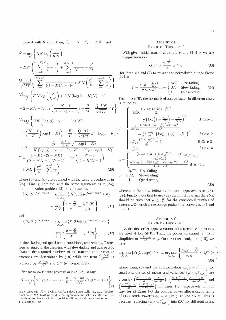
where(g) and(h) are obtained with the same procedure as in(28)6. Finally, note that with the same arguments as in (24),the optimization problem (5) is rephrased as

Nt, NrSlow-fading= argminNt,Nr

Pr(Outage)Slow-Fading≤ θ

= argNt,Nr

µ− RM

σ=

Q−1(θ)√M

(31)

and

Nt, NrQuasi-static= argminNt,Nr

Pr(Outage)Quasi-static≤ θ

= argNt,Nr

µ− RM

σ= Q−1(θ)

, (32)

in slow-fading and quasi-static conditions, respectively. There-fore, as stated in the theorem, with slow-fading and quasi-staticchannel the required numbers of the transmit and/or receiveantennas are determined by (10) while the termQ

−1(θ)√MT

is

replaced byQ−1(θ)√M

andQ−1(θ), respectively.

6We can follow the same procedure as in (28)-(29) to write

N = argN

N(log(φ) − γ − 1)− R

M=

Q−1(θ)√MT

√

log(N − 1) + 1

,

(30)

in the cases withK = 1 which can be solved numerically via, e.g., “’fsolve”function of MATLAB or by different approximation schemes. However, forsimplicity and because it is a special condition, we do not considerK = 1as a separate case.

APPENDIX BPROOF OFTHEOREM 2

With given initial transmission rateR and SNRφ, we usethe approximation

Q(x) ≃ e−x2

2

2, x ≥ 0, (33)

for largex’s and (7) to rewrite the normalized outage factor(12) as

Γ =c(

µ− RM

)2

2NtNrσ2, c =

MT, Fast-fadingM, Slow-fading1, Quasi-static.

(34)

Then, from (8), the normalized outage factor in different casesis found as

Γ =

c2NtNr

(Nt log(1+NrφNt

)− RM )

2

NtNr

= c2

(

log(

1 + NrφNt

)

− RMNt

)2

if Case 1

c2NtNr

(Nr log(1+φ)− RM )2Nt(1+φ)2

Nrφ2

= c2(1+φ)2

φ2

(

log(1 + φ)− RMNr

)2

if Case 2

c2KN2

(Nφ− RM )2

φ2

K

= c2 if Case 3

c2Kα, if Case 4

α =

(log(φ)+(K−1) log( KK−1 )−γ−1)2

log( KK−1 )

if K > 1

K2(log(φ)+K−1K

log(1−K)−log(K)−γ−1)2

− log(1−K) if K < 1,

c =

MT, Fast-fadingM, Slow-fading1, Quasi-static,

(35)

whereα is found by following the same approach as in (28)-(29). Finally, note that to use (33) the initial rate and the SNRshould be such thatµ ≥ R

Mfor the considered number of

antennas. Otherwise, the outage probability converges to 1andΓ → 0.

APPENDIX CPROOF OFTHEOREM 3

As the first order approximation, all retransmission roundsare used at low SNRs. Thus, the power constraint (17.ii) is

simplified to∑

Mi=1 φi

M= φ. On the other hand, from (15), we

have

argminNt,Nr

Pr(Outage) ≤ θ ≡ argminNt,Nr

µ(M) − RM

σ(M)≤ Q−1(θ)

,

(36)

where using (8) and the approximationlog(1 + x) ≃ x for

small x’s, the set of means and variances(

µ(M), σ2(M)

)

are

given by(

Nr∑M

i=1 φi

M, NtNrTM2

)

,(

Nr∑M

i=1 φi

M,Nr∑M

i=1 φ2i

NtTM2

)

and(

Nr∑M

i=1 φi

M,Nr∑M

i=1 φ2i

NtTM2

)

in Cases 1-3, respectively. In thisway, for all Cases 1-3, the optimal power allocation, in termsof (17), tends towardsφi = φj , ∀i, j, at low SNRs. This is

because, replacing(

µ(M), σ2(M)

)

into (36) for different cases,

14

both the objective function and the constraint of (17) aresymmetric functions ofφi, ∀i, i.e., the power termsφi, ∀i,are interchangeable in (17), at low SNRs.

REFERENCES

[1] B. Gammage, D. C. Plummer, E. Thompson, L. Fiering, H. LeHong,F. Karamouzis, C. Da Rold, K. Collins, W. Clark, N. Jones, C. Smulders,M. Escherich, M. Reynolds, and M. Basso, “Gartner’s top predictions forIT organizations and users, 2010 and beyond: A new balance,”GartnerReport, Dec. 2009.

[2] N. Bhushan, J. Li, D. Malladi, R. Gilmore, D. Brenner, A. Damnjanovic,R. Sukhavasi, C. Patel, and S. Geirhofer, “Network densification: Thedominant theme for wireless evolution into 5G,”IEEE Commun. Mag.,vol. 52, no. 2, pp. 82–89, Feb. 2014.

[3] T. S. Rappaport, S. Sun, R. Mayzus, H. Zhao, Y. Azar, K. Wang, G. N.Wong, J. K. Schulz, M. Samimi, and F. Gutierrez, “Millimeterwavemobile communications for 5G cellular: It will work!”IEEE Access,vol. 1, pp. 335–349, May 2013.

[4] Z. Pi and F. Khan, “An introduction to millimeter-wave mobile broad-band systems,”IEEE Commun. Mag., vol. 49, no. 6, pp. 101–107, June2011.

[5] B. Makki and T. Eriksson, “On hybrid ARQ and quantized CSIfeedbackschemes in quasi-static fading channels,”IEEE Trans. Commun., vol. 60,no. 4, pp. 986–997, April 2012.

[6] G. Caire and D. Tuninetti, “The throughput of hybrid-ARQprotocolsfor the Gaussian collision channel,”IEEE Trans. Inf. Theory, vol. 47,no. 5, pp. 1971–1988, July 2001.

[7] P. Wu and N. Jindal, “Performance of hybrid-ARQ in block-fadingchannels: A fixed outage probability analysis,”IEEE Trans. Commun.,vol. 58, no. 4, pp. 1129–1141, April 2010.

[8] T. V. K. Chaitanya and E. G. Larsson, “Optimal power allocation forhybrid ARQ with chase combining in i.i.d. Rayleigh fading channels,”IEEE Trans. Commun., vol. 61, no. 5, pp. 1835–1846, May 2013.

[9] H. El Gamal, G. Caire, and M. O. Damen, “The MIMO ARQ channel:Diversity-multiplexing-delay tradeoff,”IEEE Trans. Inf. Theory, vol. 52,no. 8, pp. 3601–3621, Aug. 2006.

[10] A. Chuang, et. al, “Optimal throughput-diversity-delay tradeoff inMIMO ARQ block-fading channels,”IEEE Trans. Inf. Theory, vol. 54,no. 9, pp. 3968–3986, Sept. 2008.

[11] H. Liu, L. Razoumov, N. Mandayam, and P. Spasojevic, “An optimalpower allocation scheme for the STC hybrid-ARQ over energy limitednetworks,” IEEE Trans. Wireless Commun., vol. 8, no. 12, pp. 5718–5722, Dec. 2009.

[12] K. D. Nguyen, L. K. Rasmussen, A. Guillen i Fabregas, and N. Letzepis,“MIMO ARQ with multibit feedback: Outage analysis,”IEEE Trans. Inf.Theory, vol. 58, no. 2, pp. 765–779, Feb. 2012.

[13] B. Makki, T. Svensson, T. Eriksson, and M.-S. Alouini, “Adaptive space-time coding using ARQ,”IEEE Trans. Veh. Technol., vol. 64, no. 9, pp.4331–4337, Sept. 2015.

[14] B. Makki and T. Eriksson, “On the performance of MIMO-ARQ systemswith channel state information at the receiver,”IEEE Trans. Commun.,vol. 62, no. 5, pp. 1588–1603, May 2014.

[15] K. Zheng, H. Long, L. Wang, and W. Wang, “Linear space-time precoderwith hybrid ARQ transmission,” inProc. IEEE GLOBECOM’2007,Washington, DC, USA, Nov. 2007, pp. 3543–3547.

[16] H. Huang and Z. Ding, “Ergodic capacity maximizing MIMOARQprecoder design based on channel mean information,” inProc. IEEEITAW’2008, San Diego, CA, USA, Feb. 2008, pp. 58–62.

[17] K. Zheng, H. Long, L. Wang, W. Wang, and Y. I. Kim, “Designandperformance of space-time precoder with hybrid ARQ transmission,”IEEE Trans. Veh. Technol., vol. 58, no. 4, pp. 1816–1822, May 2009.

[18] C. Shen and M. P. Fitz, “Hybrid ARQ in multiple-antenna slow fadingchannels: Performance limits and optimal linear dispersion code design,”IEEE Trans. Inf. Theory, vol. 57, no. 9, pp. 5863–5883, Sept. 2011.

[19] Y. Xie and A. J. Goldsmith, “Diversity-multiplexing-delay tradeoffs inMIMO multihop networks with ARQ,” inProc. IEEE ISIT’2010, Austin,TX, USA, June 2010, pp. 2208–2212.

[20] P. Hesami and J. N. Laneman, “Low-complexity incremental use ofmultiple transmitters in wireless communication systems,” in Proc. IEEEAllerton’2011, Monticello, IL, USA, Sept. 2011, pp. 1613–1618.

[21] T. L. Marzetta, “How much training is required for multiuser MIMO?”in Proc. IEEE Asilomar’2006, Pacific Grove, CA, USA, Oct. 2006, pp.359–363.

[22] ——, “Noncooperative cellular wireless with unlimitednumbers of basestation antennas,”IEEE Trans. Wireless Commun., vol. 9, no. 11, pp.3590–3600, Nov. 2010.

[23] H. Q. Ngo, T. L. Marzetta, and E. G. Larsson, “Analysis ofthe pilotcontamination effect in very large multicell multiuser MIMO systems forphysical channel models,” inProc. IEEE ICASSP’2011, Prague, CzechRepublic, May 2011, pp. 3464–3467.

[24] J. Jose, A. Ashikhmin, T. L. Marzetta, and S. Vishwanath, “Pilotcontamination problem in multi-cell TDD systems,” inProc. IEEEISIT’2009, Soul, South Korea, June 2009, pp. 2184–2188.

[25] K. Appaiah, A. Ashikhmin, and T. L. Marzetta, “Pilot contaminationreduction in multi-user TDD systems,” inProc. IEEE ICC’2010, CapeTown, South Africa, May 2010, pp. 1–5.

[26] J. Jose, A. Ashikhmin, T. L. Marzetta, and S. Vishwanath, “Pilotcontamination and precoding in multi-cell TDD systems,”IEEE Trans.Wireless Commun., vol. 10, no. 8, pp. 2640–2651, Aug. 2011.

[27] Z. Xiang, M. Tao, and X. Wang, “Massive MIMO multicasting innoncooperative cellular networks,”IEEE J. Sel. Areas Commun., vol. 32,no. 6, pp. 1180–1193, June 2014.

[28] B. Gopalakrishnan and N. Jindal, “An analysis of pilot contamination onmulti-user MIMO cellular systems with many antennas,” inProc. IEEESPAWC’2011, San Francisco, CA, USA, June 2011, pp. 381–385.

[29] J. Hoydis, S. ten Brink, and M. Debbah, “Massive MIMO in the UL/DLof cellular networks: How many antennas do we need?”IEEE J. Sel.Areas Commun., vol. 31, no. 2, pp. 160–171, Feb. 2013.

[30] J. Choi, D. J. Love, and P. Bidigare, “Downlink trainingtechniques forFDD massive MIMO systems: Open-loop and closed-loop training withmemory,”IEEE J. Sel. Topics Signal Process., vol. 8, no. 5, pp. 802–814,Oct. 2014.

[31] X. Rao and V. K. N. Lau, “Distributed compressive CSIT estimationand feedback for FDD multi-user massive MIMO systems,”IEEE Trans.Signal Process, vol. 62, no. 12, pp. 3261–3271, June 2014.

[32] J. Choi, Z. Chance, D. J. Love, and U. Madhow, “Noncoherent trelliscoded quantization: A practical limited feedback technique for massiveMIMO systems,”IEEE Trans. Commun., vol. 61, no. 12, pp. 5016–5029,Dec. 2013.

[33] H. Q. Ngo, E. G. Larsson, and T. L. Marzettat, “Uplink power efficiencyof multiuser MIMO with very large antenna arrays,” inProc. IEEEAllerton’2011, Monticello, IL, USA, Sept. 2011, pp. 1272–1279.

[34] H. Huh, G. Caire, H. C. Papadopoulos, and S. A. Ramprashad, “Achiev-ing massive MIMO spectral efficiency with a not-so-large number ofantennas,”IEEE Trans. Wireless Commun., vol. 11, no. 9, pp. 3226–3239, Sept. 2012.

[35] S. Wagner, R. Couillet, M. Debbah, and D. T. M. Slock, “Large systemanalysis of linear precoding in correlated MISO broadcast channelsunder limited feedback,”IEEE Trans. Inf. Theory, vol. 58, no. 7, pp.4509–4537, July 2012.

[36] E. Larsson, O. Edfors, F. Tufvesson, and T. Marzetta, “Massive MIMOfor next generation wireless systems,”IEEE Commun. Mag., vol. 52,no. 2, pp. 186–195, Feb. 2014.

[37] L. Lu, G. Y. Li, A. L. Swindlehurst, A. Ashikhmin, and R. Zhang,“An overview of massive MIMO: Benefits and challenges,”IEEE J. Sel.Topics Signal Process., vol. 8, no. 5, pp. 742–758, Oct. 2014.

[38] F. Rusek, D. Persson, B. K. Lau, E. G. Larsson, T. L. Marzetta,O. Edfors, and F. Tufvesson, “Scaling up MIMO: Opportunities andchallenges with very large arrays,”IEEE Signal Process. Mag., vol. 30,no. 1, pp. 40–60, Jan. 2013.

[39] B. M. Hochwald, T. L. Marzetta, and V. Tarokh, “Multiple-antennachannel hardening and its implications for rate feedback and scheduling,”IEEE Trans. Inf. Theory, vol. 50, no. 9, pp. 1893–1909, Sept. 2004.

[40] Y. Polyanskiy, H. V. Poor, and S. Verdu, “Channel codingrate in thefinite blocklength regime,”IEEE Trans. Inf. Theory, vol. 56, no. 5, pp.2307–2359, May 2010.

[41] W. Yang, G. Durisi, T. Koch, and Y. Polyanskiy, “Quasi-static multiple-antenna fading channels at finite blocklength,”IEEE Trans. Inf. Theory,vol. 60, no. 7, pp. 4232–4265, July 2014.

[42] mmMagic Deliverable D1.1, “Use case characterization, KPIs and pre-ferred suitable frequency ranges for future 5G systems between 6 GHzand 100 GHz,” Nov. 2015, available at: https://5g-mmmagic.eu/results/.

[43] Ericsson AB, “Delivering high-capacity and cost-efficient backhaul forbroadband networks today and in the future,” Sept. 2015, available at:http://www.ericsson.com/res/docs/2015/microwave-2020-report.pdf.

[44] B. Makki and T. Eriksson, “On the average rate of quasi-static fadingchannels with ARQ and CSI feedback,”IEEE Commun. Lett., vol. 14,no. 9, pp. 806–808, Sept. 2010.

[45] ——, “Feedback subsampling in temporally-correlated slowly-fadingchannels using quantized CSI,”IEEE Trans. Commun., vol. 61, no. 6,pp. 2282–2294, June 2013.

[46] T. M. Cover and J. A. Thomas,Elements of Information Theory. NewYork: Wiley Interscience, 1992.

15

[47] A. El Gamal and Y.-H. Kim, “Lecture notes on network informationtheory,” 2010, [Online]. Available athttp://arxiv.org/abs/1001.3404v4/.

[48] E. Bjornemo, “Energy constrained wireless sensor networks: commu-nication principles and sensing aspects,” Ph.D. dissertation, UppsalaUniversity, Uppsala, Sweden, 2009.

[49] S. Mikami, T. Takeuchi, H. Kawaguchi, C. Ohta, and M. Yoshimoto, “Anefficiency degradation model of power amplifier and the impact againsttransmission power control for wireless sensor networks,”in Proc. IEEERWS’2007, Long Beach, CA, USA, Jan. 2007, pp. 447–450.

[50] D. Persson, T. Eriksson, and E. G. Larsson, “Amplifier-aware multiple-input single-output capacity,”IEEE Trans. Commun., vol. 62, no. 3, pp.913–919, March 2014.

[51] B. Makki, A. Graell i Amat, and T. Eriksson, “On noisy ARQin block-fading channels,”IEEE Trans. Veh. Technol., vol. 63, no. 2, pp. 731–746,Feb. 2014.

[52] B. Makki, T. Svensson, and M. Zorzi, “Finite block-length analysisof the incremental redundancy HARQ,”IEEE Wireless Commun. Lett.,vol. 3, no. 5, pp. 529–532, Oct. 2014.

[53] B. E. Godana and T. Ekman, “Parametrization based limited feedbackdesign for correlated MIMO channels using new statistical models,”IEEE Trans. Wireless Commun., vol. 12, no. 10, pp. 5172–5184, Oct.2013.

[54] I. M. Kim, “Exact BER analysis of OSTBCs in spatially correlatedMIMO channels,”IEEE Trans. Commun., vol. 54, no. 8, pp. 1365–1373,Aug. 2006.

[55] A. L. Moustakas, S. H. Simon, and A. M. Sengupta, “MIMO capacitythrough correlated channels in the presence of correlated interferers andnoise: A (not so) large N analysis,”IEEE Trans. Inf. Theory, vol. 49,no. 10, pp. 2545–2561, Oct. 2003.

[56] K. S. Ahn and R. W. Heath, “Performance analysis of maximumratio combining with imperfect channel estimation in the presence ofcochannel interferences,”IEEE Trans. Wireless Commun., vol. 8, no. 3,pp. 1080–1085, Mar. 2009.

[57] R. M. Corless, G. H. Gonnet, D. E. G. Hare, D. J. Jeffrey, and D. E.Knuth, “On the Lambert W function,”Advances in ComputationalMathematics, vol. 5, pp. 329–359, 1996.

Behrooz Makki was born in Tehran, Iran. Hereceived the B.Sc. degree in Electrical Engineeringfrom Sharif University of Technology, Tehran, Iran,and the M.Sc. degree in Bioelectric Engineeringfrom Amirkabir University of Technology, Tehran,Iran, respectively. Behrooz received his PhD degreein Communication Engineering from Chalmers Uni-versity of Technology, Gothenburg, Sweden. Since2013, he is working as a Postdoc at ChalmersUniversity. Behrooz is the recipient of VR ResearchLink grant, Sweden, 2014, and the Ericsson’s Re-

search grant, Sweden, 2013, 2014 and 2015. Also, he is a member of EuropeanCommission 5G project “mm-Wave based Mobile Radio Access Network for5G Integrated Communications.” His current research interests include partialchannel state information (CSI) feedback, hybrid automatic repeat request,Green communication, millimeter wave communication, free-space opticalcommunication and finite block-length analysis.

TOMMY SVENSSON [S’98, M’03, SM’10] isAssociate Professor in Communication Systems atChalmers University of Technology in Gothenburg,Sweden, where he is leading the research on airinterface and wireless backhaul networking tech-nologies for future wireless systems. He receiveda Ph.D. in Information theory from Chalmers in2003, and he has worked at Ericsson AB with corenetworks, radio access networks, and microwavetransmission products. He was involved in the Euro-pean WINNER and ARTIST4G projects that made

important contributions to the 3GPP LTE standards, the recently finishedEU FP7 METIS 5G project and is currently involved in the EU H20205GPPP mmMAGIC project targeting mm-wave solutions for 5G. His mainresearch interests are in design and analysis of physical layer algorithms,multiple access, resource allocation, cooperative systems, moving networksand satellite networks. He has co-authored three books and more than 120journal and conference papers. He is Chairman of the IEEE Sweden jointVehicular Technology/Communications/Information Theory Societies chapter,and coordinator of the Communication Engineering Master’sProgram atChalmers.

Thomas Eriksson received the Ph.D. degree in In-formation Theory in 1996, from Chalmers Universityof Technology, Gothenburg, Sweden. From 1990 to1996, he was at Chalmers. In 1997 and 1998, he wasat AT&T Labs - Research in Murray Hill, NJ, USA,and in 1998 and 1999 he was at Ericsson RadioSystems AB, Kista, Sweden. Since 1999, he hasbeen at Chalmers University, where he is a professorin communication systems. Further, he was a guestprofessor at Yonsei University, S. Korea, in 2003-2004. He has authored and co-authored more than

200 journal and conference papers, and is the inventor of 7 patents.Prof. Ericsson is leading the research efforts on hardware-constrained

communications at Chalmers. His research interests include communication,data compression, and modeling and compensation of non-ideal hardwarecomponents (e.g. amplifiers, oscillators, modulators in communication trans-mitters and receivers, including massive MIMO). He is currently vice headof the department of Signals& Systems at Chalmers, with responsibility forundergraduate and master education.

Mohamed-Slim Alouini (S’94, M’98, SM’03, F’09)was born in Tunis, Tunisia. He received the Ph.D.degree in Electrical Engineering from the CaliforniaInstitute of Technology (Caltech), Pasadena, CA,USA, in 1998. He served as a faculty memberin the University of Minnesota, Minneapolis, MN,USA, then in the Texas A&M University at Qatar,Education City, Doha, Qatar before joining KingAbdullah University of Science and Technology(KAUST), Thuwal, Makkah Province, Saudi Arabiaas a Professor of Electrical Engineering in 2009.

His current research interests include the modeling, design, and performanceanalysis of wireless communication systems.