cfd simulation study on the effect of …umpir.ump.edu.my/9239/1/cd8690.pdf · water velocity...

III

CFD SIMULATION STUDY ON THE EFFECT OF

WATER VELOCITY TOWARDS OIL LEAKAGE

FROM SUBMARINE PIPELINES

AMARASINGAM A/L SELVARAJAH

Thesis submitted in partial fulfilment of the requirements

for the award of the degree of

Bachelor of Chemical Engineering (Gas Technology)

Faculty of Chemical & Natural Resources Engineering

UNIVERSITI MALAYSIA PAHANG

JULY 2014

©AMARASINGAM A/L SELVARAJAH (2014)

VIII

ABSTRACT

This paper presents Computational fluid dynamic (CFD) studies on water velocity effect

towards the time taken for migration of oil droplets to reach free surface. Computational

Fluid Dynamic (CFD) simulations with FLUENT software 6.3.26 were simulated to

detect the leakage process of oil spill from submarine pipeline to free surface. GAMBIT

2.4.6 mesh-generator is employed to perform all geometry generation and meshing. The

velocity inlet of water (vs.) was varied whereas density of oil (kerosene liquid) was

constant at 780kg/m3 .A computational rectangular domain with length of 20m and

height of 15m was simulated in Gambit 2.4.6. The mesh was generated and exported to

Fluent. In the Fluent 6.3.26, the time taken for the oil droplets to reach free surface was

observed by varying water inlet velocity; vw1=0.02m/s, vw2=0.04m/s,vw3=0.08m/s

respectively. Kerosene droplets reached free surface faster as the velocity of water inlet

increased. Results were observed at 1000 number of time steps (iterations) with a step

size of 0.1seconds. The leak size was shown to be 0.1meter, which was fixed at the

beginning of the simulation conditions. Justifications were shown where oil droplets

released from a greater leak width are easier to collision and have greater chance of

gathering into large droplets, (Zhu et al., 2013). This is because at a larger face of

leakage, the shear stresses increases, causing a larger displacement in oil migration.

From the study, the dimensionless longest horizontal distance the kerosene droplets

migrate when they reach the sea surface are analysed and the fitting formulas are

obtained. With this, the maximum horizontal migration distance of oil at certain time is

predicted, and a forecasting model is proposed in order to place the oil containment

boom. This helps to detect the leakage more accurately and reduces cost of handling.

Key words: Computational fluid dynamic (CFD), computational domain, Gambit 2.4.6

and Fluent 6.3.26, Water velocity

IX

TABLE OF CONTENTS

STUDENT’S DECLARATION ...................................................................................... V

Dedication ....................................................................................................................... VI

ACKNOWLEDGEMENT ............................................................................................. VII

ABSTRACT................................................................................................................. VIII

LIST OF FIGURES ........................................................................................................ XI

LIST OF TABLES ......................................................................................................... XII

LIST OF ABBREVIATIONS ...................................................................................... XIII

1 INTRODUCTION .................................................................................................... 1

1.0 Brief introduction and problem statement.......................................................... 1

1.1 Motivation .......................................................................................................... 2

1.2 Objectives of Study ............................................................................................ 3

1.3 Scope of this research......................................................................................... 3

1.4 Hypothesis .......................................................................................................... 4

1.5 Main contribution of this work .......................................................................... 4

1.6 Organisation of thesis ......................................................................................... 4

2 LITERATURE REVIEW ......................................................................................... 5

2.0 Screening Route ................................................................................................. 5

2.1 Oil Leakage ........................................................................................................ 5

2.2 Computational Fluid Dynamics (CFD) .............................................................. 7

2.2.1 Oil Spillage ................................................................................................. 7

2.2.2 Experiments versus Simulations ............................................................... 11

2.2.3 The Finite Volume Method....................................................................... 11

2.3 Multiphase Flow Theory .................................................................................. 12

2.3.1 VOF Model Approach .............................................................................. 12

2.4 Software ........................................................................................................... 12

2.4.1 ICEM CFD ................................................................................................ 12

2.4.2 Fluent ........................................................................................................ 13

2.5 Computational Domain and Mesh ................................................................... 13

2.6 Effect of oil density on Oil spills ..................................................................... 14

3 MATERIALS AND METHODS............................................................................ 17

3.1 Overview .......................................................................................................... 17

3.2 Simulation Methodology .................................................................................. 17

3.2.1 Governing equations ................................................................................. 17

3.2.2 Computational Domain and Mesh ............................................................ 18

3.3 Effects of variables on the Oil Spill Process .................................................... 20

3.3.1 Effects of oil density ................................................................................. 20

3.3.2 Effect of oil leaking rate ........................................................................... 21

3.3.3 Effect of oil leak size ................................................................................ 21

3.3.4 Effect of water velocity............................................................................. 22

3.4 Summary .......................................................................................................... 22

4 RESULTS & DISCUSSIONS ................................................................................ 23

4.1 Overview .......................................................................................................... 23

4.2 Results and Discussions ................................................................................... 23

X

4.3 Statistical analysis ............................................................................................ 38

4.4 Summary .......................................................................................................... 39

5.0 CONCLUSION ................................................................................................ 40

5.1 Conclusion ....................................................................................................... 40

5.2 Future work ...................................................................................................... 40

6.0 REFERENCES ................................................................................................. 41

XI

LIST OF FIGURES

Figure 2-1: Fluent Simulation using k-epsilon turbulence model. (Shehadeh et al., 2012)

..........................................................................................................................10

Figure 2-2: Distribution of oil-water-gas (t = 56s, u = 0.1m/s, P = 101000pa) (Li et al.,

2013) ..................................................................................................................15


2013) ..................................................................................................................15


2013) ..................................................................................................................16


2013) ..................................................................................................................16

Figure 3-1: Sketch of the geometry and numerical grid for computational domain: (a)

overall view of the computational domain and boundary conditions; (b) grid distribution

of computational domain. (Zhu et al. 2013) ............................................................19

Figure 4-1: Process of oil spill to free surface from damaged submarine pipelines at

water velocity of 0.08m/s. .....................................................................................24





Figure 4-4: Comparison of water velocity (m/s) towards time(s) of leakage from

pipeline. ..............................................................................................................30

Figure 4-5: Comparison of water velocity (m/s) towards time(s) of leakage ...............32



Figure 4-7Comparison of water velocity; 0.04 m/s for both from results and ..............36

XII

LIST OF TABLES

Table 2-1: The factors of how oil spill can occur from damaged submarine pipeline .... 6

Table 2-2: Oil Spills of 100,000 Tons (640,000 Barrels), or More .............................. 7

Table 2-3: CFD Modeling Scenarios; Alexander, C. (2005) ....................................... 8

Table 2-4: CFD contour plots with continuous leaking at 240 ft3/dayAlexander, C.

(2005) ................................................................................................................. 9

Table 2-5: Parameters used in the Fluent Simulation (Shehadehet al., 2012). .............10

Table 2-6: Comparison of experimental and simulation runs (Wesselling et al., 2001) .11

Table 2-7:Simulation cases, in which variables of oil density, oil leaking rate, diameter

of leak, and maximum water velocity are varied ( Zhu et al., 2013) ...........................14

Table 3-1: Simulation cases, in which parameters are varied in recent findings. ..........22

Table 4-1: Time taken(s) for oil to reach free surface with varying water velocities (m/s)

..........................................................................................................................38

XIII

LIST OF ABBREVIATIONS

Greek

vl kinematic viscosity

µm micrometre

m/s Water velocity / oil leaking rate

m3/s Volume flux

wt % moisture content

KJ/kg Calorific Value

Kg/m3 oil density

Pa.s Pascal .seconds

Diameters (height, distance)

ρ density

g gravity

CFD Computational Fluid Dynamics

RANS (Reynolds-Averaged-Navier-Stokes) equations,

VOF Volume of Fluid

FVM (finite volume method)

MESH 2.4.6

FLUENT 6.3.26

1

1 INTRODUCTION

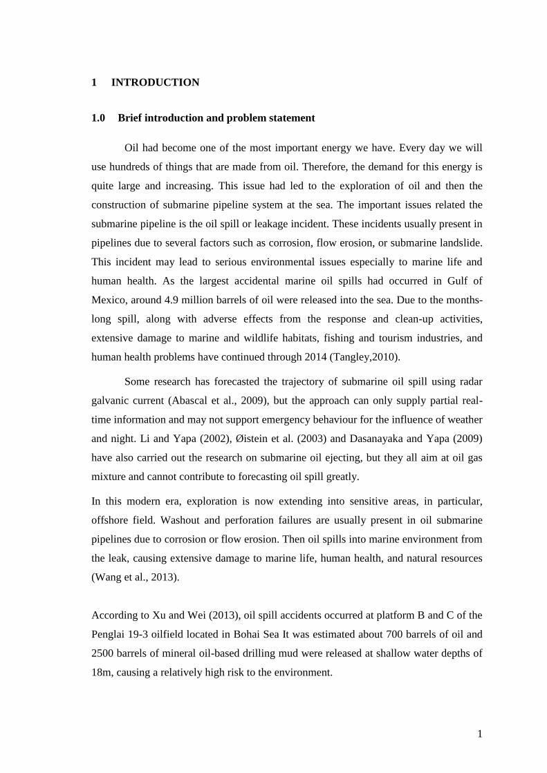
1.0 Brief introduction and problem statement

Oil had become one of the most important energy we have. Every day we will

use hundreds of things that are made from oil. Therefore, the demand for this energy is

quite large and increasing. This issue had led to the exploration of oil and then the

construction of submarine pipeline system at the sea. The important issues related the

submarine pipeline is the oil spill or leakage incident. These incidents usually present in

pipelines due to several factors such as corrosion, flow erosion, or submarine landslide.

This incident may lead to serious environmental issues especially to marine life and

human health. As the largest accidental marine oil spills had occurred in Gulf of

Mexico, around 4.9 million barrels of oil were released into the sea. Due to the months-

long spill, along with adverse effects from the response and clean-up activities,

extensive damage to marine and wildlife habitats, fishing and tourism industries, and

human health problems have continued through 2014 (Tangley,2010).

Some research has forecasted the trajectory of submarine oil spill using radar

galvanic current (Abascal et al., 2009), but the approach can only supply partial real-

time information and may not support emergency behaviour for the influence of weather

and night. Li and Yapa (2002), Øistein et al. (2003) and Dasanayaka and Yapa (2009)

have also carried out the research on submarine oil ejecting, but they all aim at oil gas

mixture and cannot contribute to forecasting oil spill greatly.

In this modern era, exploration is now extending into sensitive areas, in particular,

offshore field. Washout and perforation failures are usually present in oil submarine

pipelines due to corrosion or flow erosion. Then oil spills into marine environment from

the leak, causing extensive damage to marine life, human health, and natural resources

(Wang et al., 2013).

According to Xu and Wei (2013), oil spill accidents occurred at platform B and C of the

Penglai 19-3 oilfield located in Bohai Sea It was estimated about 700 barrels of oil and

2500 barrels of mineral oil-based drilling mud were released at shallow water depths of

18m, causing a relatively high risk to the environment.

2

Once accidental oil leakages occur, a quick and adequate response in order to reduce the

environmental consequences is required. (Biksey et al., 2010). Besides, laying oil

containment boom, as a basic way to control oil dispersal, also depends on the rising

velocity of oil droplets and the trend of spreading. Therefore, an exact prediction of oil

spill process and dispersal could provide useful information for setting up oil

containment boom and reducing the damage of future oil spills. (Hongjun et al., 2014)

An effective attempt has been made to observe the oil spill under the action of current

and wave. However, the velocity of current in their study was uniform, which does not

match with the actual shear velocity distribution under sea surface. And the actual

hydrostatic pressure distribution was not used in their modelling. Moreover, the crucial

parameter, the maximum horizontal migration distance of oil, was not considered in

their research. (Li et al., 2013)

1.1 Motivation

The increasing oil spill accidents from submarine pipelines have caused severe

damage to the aquatic life and health problems to mankind. A lot of research had been

made manually and by simulation to study the effective measure in detecting a leakage.

Because of the oil leakage from damaged submarine pipeline, the migration of oil flow

along the depth direction is an important issue to address.

Hence, numerical simulation can provide detailed information on the

hydrodynamics of oil flow, which is not easily obtained by physical experiments. CFD

(computational fluid dynamic) model coupling with VOF (volume of fluid) method has

been used to investigate the process of oil spill from submarine pipeline to free surface.

The actual shear velocity distribution of current and the actual hydrostatic pressure

distribution are considered in this study.

Detailed oil droplet and sea-surface in-formation could be obtained by the VOF

model. By conducting a series of numerical simulations, effects of oil density, oil

leaking rate, leak size and water velocity on the oil spill process are examined. Then, the

dimensionless time required for oil droplets which have the longest horizontal migrate

distance when they reach the sea surface and the dimensionless longest horizontal

3

distance the droplets migrate when they reach the sea surface are analyzed and the

fitting formulas are obtained.( Yadav et al.,2013 ; Arpino et al.,2009 ; Jalilinasrabady et

al.,2013).

Summary

The topic was scoped from addressing the problem in the petroleum industry, way by

identifying the problem of leakage in submarine pipelines.Then, an alternative solution

using the CFD (computational fluid dynamic) model coupling with VOF (volume of

fluid) method has been used to investigate the process of oil spill from submarine

pipeline to free surface.

1.2 Objectives of Study

The main objective of this study is to investigate the time taken for oil droplets(s) to

migrate along a horizontal distance up to free surface with varying water velocities

(m/s) using the Gambit 2.4.6 and Fluent 6.3.26.

1.3 Scope of this research

The scopes of this study are to mainly study the effects of water velocity on the oil spill

process. The method of study is by implementing computational fluid dynamics using

the Gambit 2.4.6 and the Fluent Software. GAMBIT 2.4.6 mesh-generator is employed

to perform all geometry generation and meshing. The whole computational domain is a

rectangle with a length of 20 m and a height of 15 m. The length of computational

domain is large enough, which is larger than the longest horizontal distance the oil

droplets migrate when they reach the sea surface. Water occupies the lower region with

height of 14.5 m, while air occupies the upper region. The damaged submarine pipe

with the outer diameter (D) of 0.6 m at both sides. . In the Fluent 6.3.26, the time taken

for the oil droplets to reach free surface was observed by varying water inlet velocity;

vw1=0.02m/s, vw2=0.04m/s,vw3=0.08m/s respectively. Kerosene droplets reached free

surface faster as the velocity of water inlet increased. Results were observed at 1000

number of time steps (iterations) with a step size of 0.1s.

4

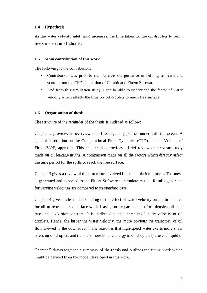
1.4 Hypothesis

As the water velocity inlet (m/s) increases, the time taken for the oil droplets to reach

free surface is much shorter.

1.5 Main contribution of this work

The following is the contribution:

• Contribution was prior to our supervisor’s guidance in helping us learn and

venture into the CFD simulation of Gambit and Fluent Software.

• And from this simulation study, I can be able to understand the factor of water

velocity which affects the time for oil droplets to reach free surface.

1.6 Organisation of thesis

The structure of the reminder of the thesis is outlined as follow:

Chapter 2 provides an overview of oil leakage in pipelines underneath the ocean. A

general description on the Computational Fluid Dynamics (CFD) and the Volume of

Fluid (VOF) approach. This chapter also provides a brief review on previous study

made on oil leakage myths. A comparison made on all the factors which directly affect

the time period for the spills to reach the free surface.

Chapter 3 gives a review of the procedure involved in the simulation process. The mesh

is generated and exported to the Fluent Software to simulate results. Results generated

for varying velocities are compared to its standard case.

Chapter 4 gives a clear understanding of the effect of water velocity on the time taken

for oil to reach the sea-surface while leaving other parameters of oil density, oil leak

rate and leak size constant. It is attributed to the increasing kinetic velocity of oil

droplets. Hence, the larger the water velocity, the more obvious the trajectory of oil

flow skewed to the downstream. The reason is that high-speed water exerts more shear

stress on oil droplets and transfers more kinetic energy to oil droplets (kerosene liquid).

Chapter 5 draws together a summary of the thesis and outlines the future work which

might be derived from the model developed in this work.

5

2 LITERATURE REVIEW

2.0 Screening Route

My literature study was on the oil leakage in submarine pipelines which endanger the

environment and aquatic life. In addition, research was also completed on

Computational Fluid Dynamics (CFD). The study conducted did not neglect the

environmental aspects and economy imprecision. Finally, the literature centered on the

effect of water velocity towards oil migration in a horizontal distance to the free surface.

2.1 Oil Leakage

Over the past few decades, several major U.S. oil spills have had lasting repercussions

that transcended the local environmental and economic effects. The April 2010 oil spill

in the Gulf of Mexico has intensified interest in many oil spill-related issues. Prior to the

2010 Gulf spill, the most notable example was the 1989 Exxon Valdez spill, which

released approximately 11 million gallons (260,000 barrels) of crude oil into Prince

William Sound, Alaska. The Exxon Valdez spill produced extensive consequences

beyond Alaska. According to the National Academies of Science, the Exxon Valdez

disaster caused “fundamental changes in the way the U.S. public thought about oil, the

oil industry, and the transport of petroleum products by tankers ‘big oil’ was suddenly

seen as a necessary evil, something to be feared and mistrusted; Jonathan L (2012)

Offshore production constitutes a major portion of the overall oil and gas production.

Offshore oil and gas production is more challenging than land-based installations due to

the remote and harsher environment. Other than the production challenges,

environmental risks due to oil spills pose major challenges. An “oil spill” usually refers

to an event that led to a release of liquid petroleum hydrocarbon into the environment

due to human activity and is a form of pollution. Oil spills usually include releases of

crude oil from tankers, offshore platforms, drilling rigs and wells, as well as spills of

refined petroleum products (such as gasoline, diesel) and their by-products, and heavier

fuels used by large ships such as bunker fuel, or the spill of any oily white substance

refuse or waste oil. Spills may take months or even years to clean up. (Agrawal et al.,

2011)

6

There are several factors that may cause the oil spill from submarine pipeline.

Table 2-1: The factors of how oil spill can occur from damaged submarine pipeline

Factor Explanation Author

Submari

ne

landslid

e

This is happen due to high of sedimentation rates and

usually occurs on steeper slopes. This landslide can be

triggered by earthquakes in the sea. When the soil around

the piping system is subjected to a slide, and give the result

of displacement at high angle to the pipeline, the pipe will

severe bending. This will cause tensile failure.

Palmer

& King

(2008)

Ice

issues

This happen to submarine pipeline system in low

temperature water especially in freezing waters. In this

case, the floating ice features often drift into shallower

water. Therefore their keel comes into contact with the

seabed. When this condition happen, they will scoop the

seabed and came hit the pipeline

Croasdal

e K.

(2013)

Stamukhi can also damage the submarine pipeline system.

Stamukhi is a grounded accumulation of sea ice rubble that

typically develops along the boundary between fast ice and

the drifting pack ice. This stamukhi will exert high local

stresses on the pipeline system to inducing the excessive

bending.

Croasdal

e K.

(2013)

Ship

anchors

Ship anchors are a potential threat to submarine pipelines,

especially near harbours. This anchor will give high

damage to the pipeline due to their massive weight.

Corrosio

n

For small size lines, additionally, failures due to external

corrosion were more frequent compare than internal

corrosion. However in medium and large-size lines,

failures due to internal corrosion were more frequent than

those due to external corrosion.

J. S.

Mandke

(1990)

7

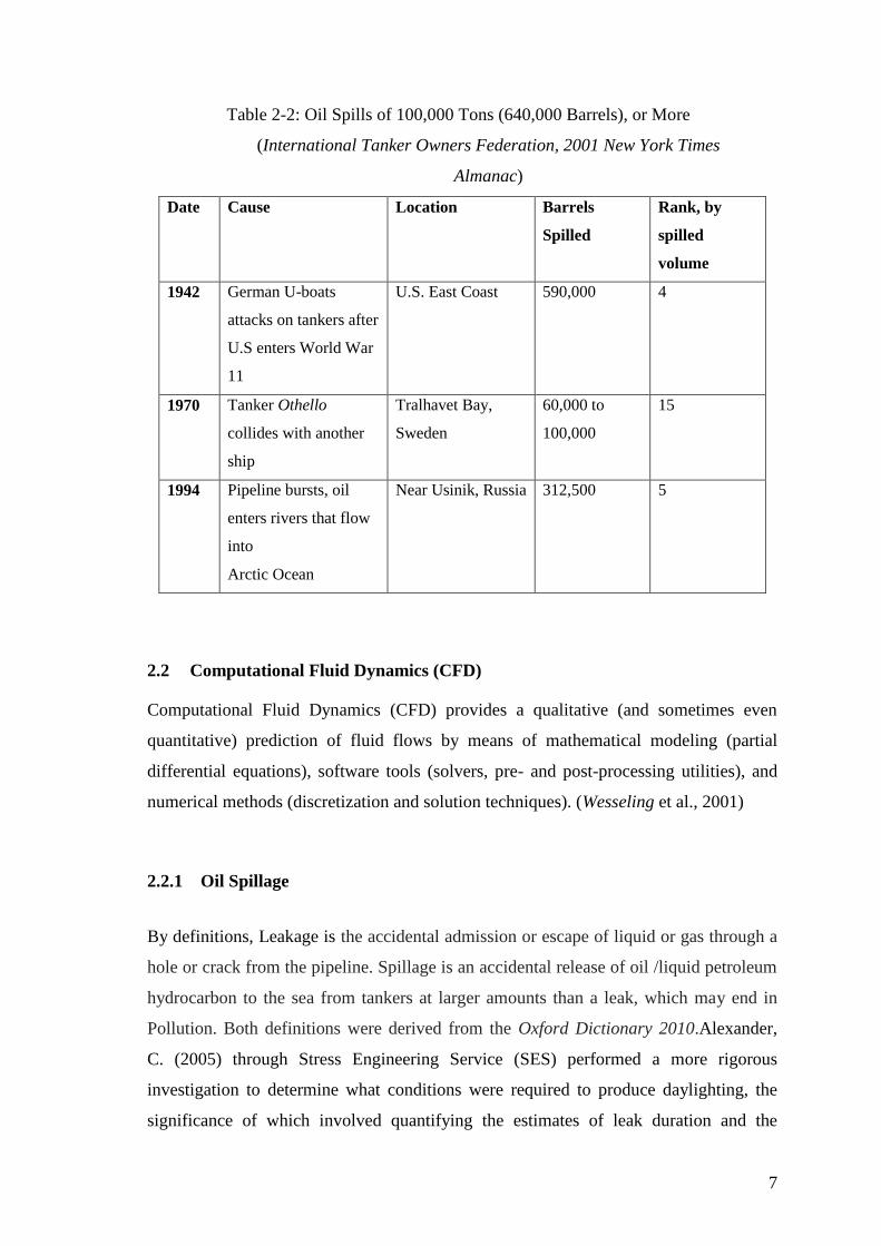
Table 2-2: Oil Spills of 100,000 Tons (640,000 Barrels), or More

(International Tanker Owners Federation, 2001 New York Times

Almanac)

2.2 Computational Fluid Dynamics (CFD)

Computational Fluid Dynamics (CFD) provides a qualitative (and sometimes even

quantitative) prediction of fluid flows by means of mathematical modeling (partial

differential equations), software tools (solvers, pre- and post-processing utilities), and

numerical methods (discretization and solution techniques). (Wesseling et al., 2001)

2.2.1 Oil Spillage

By definitions, Leakage is the accidental admission or escape of liquid or gas through a

hole or crack from the pipeline. Spillage is an accidental release of oil /liquid petroleum

hydrocarbon to the sea from tankers at larger amounts than a leak, which may end in

Pollution. Both definitions were derived from the Oxford Dictionary 2010.Alexander,

C. (2005) through Stress Engineering Service (SES) performed a more rigorous

investigation to determine what conditions were required to produce daylighting, the

significance of which involved quantifying the estimates of leak duration and the

Date Cause Location Barrels

Spilled

Rank, by

spilled

volume

1942 German U-boats

attacks on tankers after

U.S enters World War

11

U.S. East Coast 590,000 4

1970 Tanker Othello

collides with another

ship

Tralhavet Bay,

Sweden

60,000 to

100,000

15

1994 Pipeline bursts, oil

enters rivers that flow

into

Arctic Ocean

Near Usinik, Russia 312,500 5

8

petroleum volumes at Houston, Texas. This effort integrated assumptions and data from

prior analyses to assess the effects of time-dependency using computational fluid

dynamics (CFD) modeling techniques.

Table 2-3: CFD Modeling Scenarios; Alexander, C. (2005)

Scenario Description Volume of product

released

Daylight

(YES or NO)

1 Continuous leaking (330

hours)

24685 gallons

240 ft3/day-330

hours

YES

2 Leak rates based on tabulated

existing data considering two

different pressure levels

a. Pipeline beginning pressure

(667 hours)

b. Static head end pressure

(667 hours)

4,940 gallons (a)

6,212 gallons (b)

NO (a)

NO(b)

9

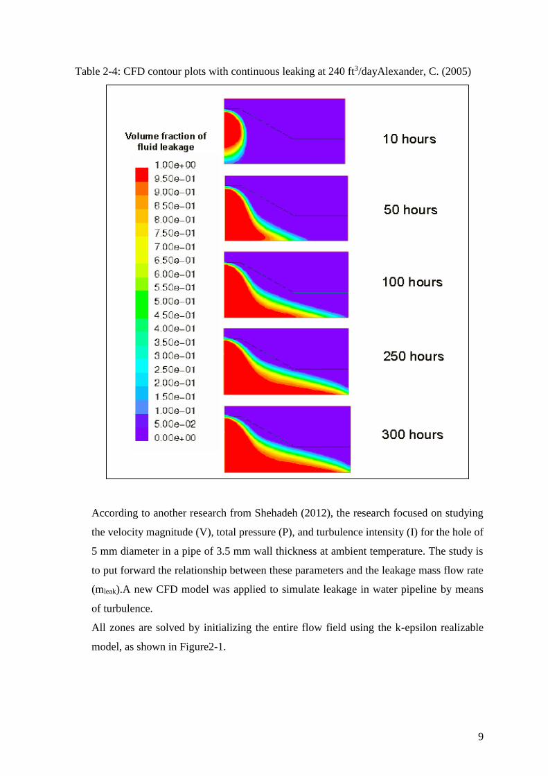
Table 2-4: CFD contour plots with continuous leaking at 240 ft3/dayAlexander, C. (2005)

According to another research from Shehadeh (2012), the research focused on studying

the velocity magnitude (V), total pressure (P), and turbulence intensity (I) for the hole of

5 mm diameter in a pipe of 3.5 mm wall thickness at ambient temperature. The study is

to put forward the relationship between these parameters and the leakage mass flow rate

(mleak).A new CFD model was applied to simulate leakage in water pipeline by means

of turbulence.

All zones are solved by initializing the entire flow field using the k-epsilon realizable

model, as shown in Figure2-1.

10

Figure 2-1: Fluent Simulation using k-epsilon turbulence model. (Shehadeh et al., 2012)

Table 2-5 below depicts on the parameters used to run the fluent software in detecting

water leakage.

Table 2-5: Parameters used in the Fluent Simulation (Shehadehet al., 2012).

Scenari

o

Vin

(m/s)

Pout(

kPa

)

Min

kg/s

Mleak

in

kg/s

Mout in

kg/s

Vm/s P(kP

a)

I(%)

1 2.7 100 5.96 0.1 5.86 Min 0 91.3 22.8

Max 6.9

3

150.9

2

246.8

2 3.2 130 7.13 0.17 6.96 Min 0 81.62 26.9

Max 11.

23

249.0

1

369.7

3 3.7 155 8.24 0.22 8.02 Min 0 75.12 31.3

11

Max 14.

2

340.0

9

462.0

Hence, the turbulence intensity has a great effect on monitoring of pipeline, for instance

leakage using novel technique such as acoustic emission [15] and ultrasonic techniques

[16].The study has predicted correlations between the mass flow rate of the

leakage and the various parameters of the pipeline system.

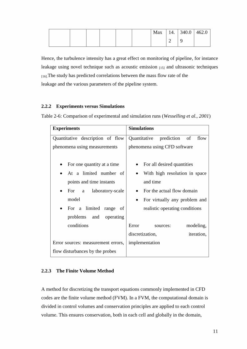
2.2.2 Experiments versus Simulations

Table 2-6: Comparison of experimental and simulation runs (Wesselling et al., 2001)

2.2.3 The Finite Volume Method

A method for discretizing the transport equations commonly implemented in CFD

codes are the finite volume method (FVM). In a FVM, the computational domain is

divided in control volumes and conservation principles are applied to each control

volume. This ensures conservation, both in each cell and globally in the domain,

Experiments Simulations

Quantitative description of flow

phenomena using measurements

For one quantity at a time

At a limited number of

points and time instants

For a laboratory-scale

model

For a limited range of

problems and operating

conditions

Error sources: measurement errors,

flow disturbances by the probes

Quantitative prediction of flow

phenomena using CFD software

For all desired quantities

With high resolution in space

and time

For the actual flow domain

For virtually any problem and

realistic operating conditions

Error sources: modeling,

discretization, iteration,

implementation

12

which is a great advantage of the FVM? Using FVM also allows for the use of

unstructured grids which decreases the computational time. (Stenmark et al., 2013)

2.3 Multiphase Flow Theory

Multiphase flow is flow with simultaneous presence of different phases, where phase

refers to solid, liquid or vapor state of matter. There are four main categories of

multiphase flows; gas-liquid, gas-solid, liquid-solid and three-phase flows.

(Thome, (2004))

2.3.1 VOF Model Approach

A third modeling approach is the volume of fluid (VOF) method. VOF belongs to the

Euler-Euler framework where all phases are treated as continuous, but in contrary to

the previous presented models the VOF model does not allow the phases to be

interpenetrating. The VOF method uses a phase indicator function, sometimes also

called a colour function, to track the interface between two or more phases. The

indicator function has value one or zero when a control volume is entirely filled with

one of the phases and a value between one and zero if an interface is present in the

control volume. Hence, the phase indicator function has the properties of volume

fraction. The transport equations are solved for mixture properties without slip velocity,

meaning that all field variables are assumed to be shared between the phases. To track

the interface, an advection equation for the indicator function is solved. In order to

obtain a sharp interface the discretization of the indicator function equation is crucial.

(Stenmark et al., 2013)

2.4 Software

For geometry and mesh generation the ANSYS software ICEM CFD was used.

2.4.1 ICEM CFD

ICEM CFD is meshing software. It allows for the use of CAD geometries or to build

the geometry using a number of geometry tools. In ICEM CFD a block-structured

meshing approach is employed, allowing for hexahedral meshes also in rather

13

complex geometries. Both structured and unstructured meshes can be created using

ICEM CFD. (Stenmark et al., 2013)

2.4.2 Fluent

The Fluent solver is based on the centre node FVM discretization technique and offers

both segregated and coupled solution methods. Three Euler-Euler multiphase models

are available; the Eulerian model, the mixture model and the VOF model. In addition,

one particle tracking model is available.

As mentioned in Section 2.3.1, the discretization of the volume fraction equation is

crucial in a VOF method to keep the interface sharp. The choice of discretization

method can have a great influence on the results in other multiphase models as well.

To resolve this issue, Fluent has a number of discretization techniques implemented

specifically for the volume fraction equation. Several methods are also available for

spatial discretization of the other transport equations.

To model interphase transfer there is both a number of drag models available along with

other transfer mechanisms such as lift forces and turbulent dispersion Fluent offers three

main approaches to model dispersed phases with a two-fluid formulation. With the

default settings it is assumed that the dispersed phase has a constant diameter or a

diameter defined by a user-defined function. With this setting, phenomena such as

coalescence and breakage are not considered. (Stenmark et al., 2013)

2.5 Computational Domain and Mesh

A sketch of the geometry (a) and numerical grid for computational domain (b)

investigated in this study. GAMBIT 2.4 mesh-generator is employed to perform all

geometry generation and meshing. The whole computational domain is a rectangle with

a length of 20 m and a height of 15 m. The length of computational domain is large

enough, which is larger than the longest horizontal distance the oil droplets migrate

when they reach the sea surface. Water occupies the lower region with height of 14.5 m,

while air occupies the upper region. In the computational domain, the damaged

submarine pipe with the outer diameter (D) of 0.6 m on both sides, the most common

14

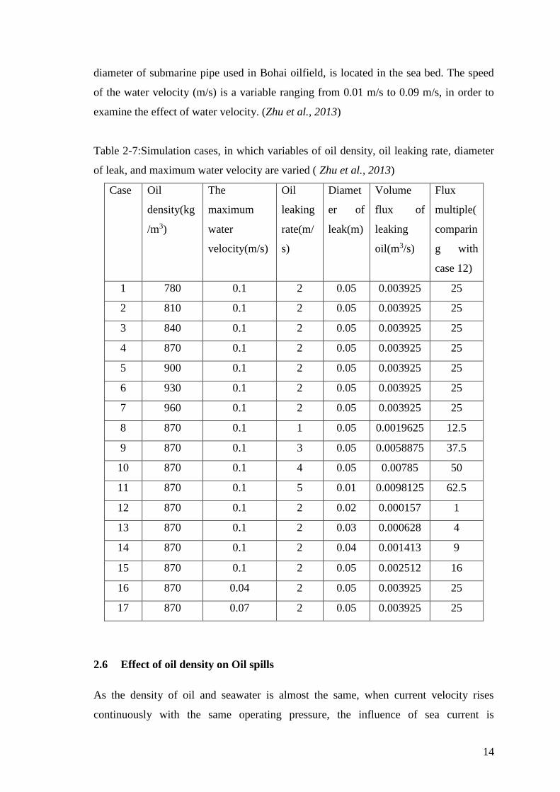
diameter of submarine pipe used in Bohai oilfield, is located in the sea bed. The speed

of the water velocity (m/s) is a variable ranging from 0.01 m/s to 0.09 m/s, in order to

examine the effect of water velocity. (Zhu et al., 2013)

Table 2-7:Simulation cases, in which variables of oil density, oil leaking rate, diameter

of leak, and maximum water velocity are varied ( Zhu et al., 2013)

Case Oil

density(kg

/m3)

The

maximum

water

velocity(m/s)

Oil

leaking

rate(m/

s)

Diamet

er of

leak(m)

Volume

flux of

leaking

oil(m3/s)

Flux

multiple(

comparin

g with

case 12)

1 780 0.1 2 0.05 0.003925 25

2 810 0.1 2 0.05 0.003925 25

3 840 0.1 2 0.05 0.003925 25

4 870 0.1 2 0.05 0.003925 25

5 900 0.1 2 0.05 0.003925 25

6 930 0.1 2 0.05 0.003925 25

7 960 0.1 2 0.05 0.003925 25

8 870 0.1 1 0.05 0.0019625 12.5

9 870 0.1 3 0.05 0.0058875 37.5

10 870 0.1 4 0.05 0.00785 50

11 870 0.1 5 0.01 0.0098125 62.5

12 870 0.1 2 0.02 0.000157 1

13 870 0.1 2 0.03 0.000628 4

14 870 0.1 2 0.04 0.001413 9

15 870 0.1 2 0.05 0.002512 16

16 870 0.04 2 0.05 0.003925 25

17 870 0.07 2 0.05 0.003925 25

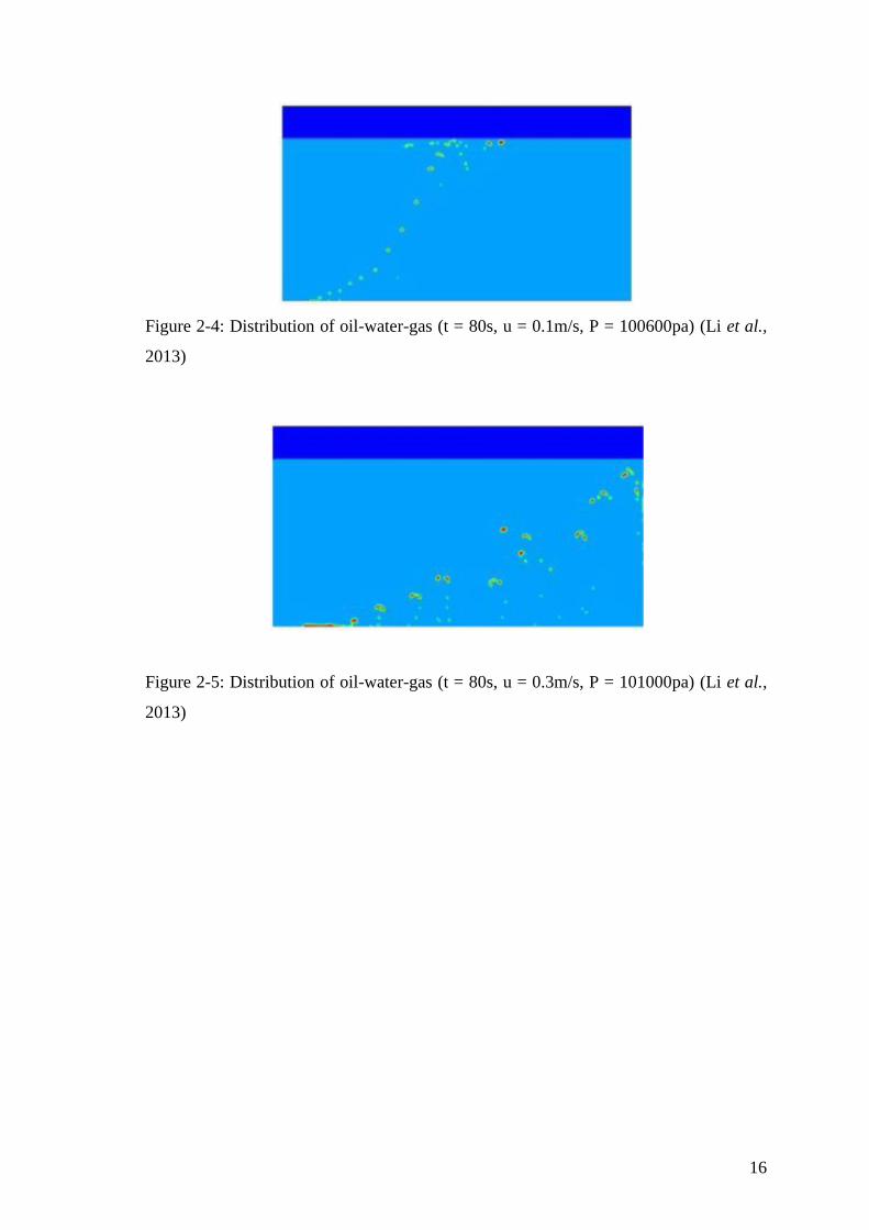
2.6 Effect of oil density on Oil spills

As the density of oil and seawater is almost the same, when current velocity rises

continuously with the same operating pressure, the influence of sea current is

15

strengthened. Meanwhile, the influence of buoyancy is relatively weakened. When the

current velocity is low (u = 0.1m/s), as shown in Fig. 2-2, the influence of buoyancy

becomes dominant to the rising spilled oil. When the current velocity is u = 0.3, u = 0.5

and u = 0.8 m/s, respectively as shown in Fig. 2-3 to 2-5, the influence of sea current

dominates obviously and oil particles move with sea current after spilled immediately.

Therefore, the higher current velocity is, the longer submarine drift distance is with its

respective densities. (Li et al., 2013)


2013)


2013)

16


2013)


2013)

17

3 MATERIALS AND METHODS

3.1 Overview

This paper is about to study the oil flows from damaged submarine pipelines with

different water velocities. First and foremost, CFD (computational fluid dynamic)

model coupling with VOF (volume of fluid) method has been used to investigate the

process of oil spill from submarine pipeline to free surface. The actual shear velocity

distribution of current and the actual hydrostatic pressure distribution are considered in

this study. Detailed oil droplet and sea-surface in-formation could be obtained by the

VOF model. Effects of oil density, oil leaking rate, leak size and water velocity on the

oil spill process are examined.

3.2 Simulation Methodology

3.2.1 Governing equations

The VOF approach is based on the solution of one momentum equation for the mixture

of the phases, and one equation for the volume fraction of fluid. In this study, volume

of fluid functions Fw and Fo are introduced to define the water region and the oil region,

respectively. The physical meaning of the F function is the fractional volume of a cell

occupied by the liquid phase. For example, a unit vale of Fw corresponds to a cell full of

water, while a zero value indicates that the cell contains no water. The fraction functions

Fw and Fo are described as follows:

𝑭𝒘=𝑽𝒘

𝑽𝒄 Equation 3.2(a)

𝑭𝒐=𝑽𝒐

𝑽𝒄 Equation 3.2(b)

where Fo and Fw are oil and water fractional function, respectively, Vc, Vo and Vw

represent volume of a cell, volume of oil inside the cell and volume of water inside the

cell, respectively.

18

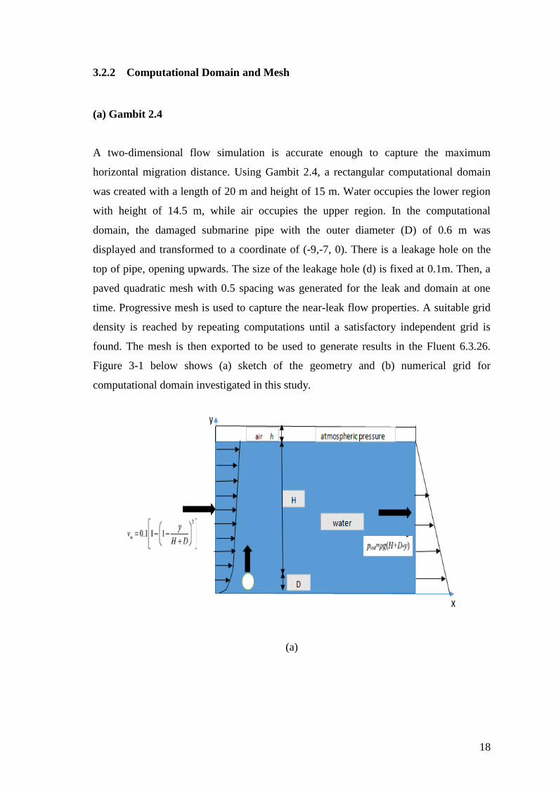
3.2.2 Computational Domain and Mesh

(a) Gambit 2.4

A two-dimensional flow simulation is accurate enough to capture the maximum

horizontal migration distance. Using Gambit 2.4, a rectangular computational domain

was created with a length of 20 m and height of 15 m. Water occupies the lower region

with height of 14.5 m, while air occupies the upper region. In the computational

domain, the damaged submarine pipe with the outer diameter (D) of 0.6 m was

displayed and transformed to a coordinate of (-9,-7, 0). There is a leakage hole on the

top of pipe, opening upwards. The size of the leakage hole (d) is fixed at 0.1m. Then, a

paved quadratic mesh with 0.5 spacing was generated for the leak and domain at one

time. Progressive mesh is used to capture the near-leak flow properties. A suitable grid

density is reached by repeating computations until a satisfactory independent grid is

found. The mesh is then exported to be used to generate results in the Fluent 6.3.26.

Figure 3-1 below shows (a) sketch of the geometry and (b) numerical grid for

computational domain investigated in this study.

(a)

cfd simulation study on the effect of …umpir.ump.edu.my/9239/1/cd8690.pdf · water velocity...

Documents