1

Prediction of Wave-Induced Scour Depth under Submarine Pipelines

Using Machine Learning Approach

A. Etemad-Shahidi *, R. Yasa, M.H. Kazeminezhad

School of Civil Engineering, Iran University of Science and Technology, Tehran, Iran,

P.O. Box 16765-163, Tel.: +9821 77240399, Fax: +9821 77240398.

* Corresponding Author, E-mail: etemad@iust.ac.ir

Abstract

The scour around submarine pipelines may influence their stability; therefore scour prediction is

a very important issue in submarine pipelines design. Several investigations have been conducted to

develop a relationship between wave-induced scour depth under pipelines and the governing parameters.

However, existing formulas do not always yield accurate result due to the complexity of the scour

phenomenon. Recently, machine learning approaches such as Artificial Neural Networks

(ANNs) have been used to increase the accuracy of the scour depth prediction. Nevertheless,

they are not as transparent and easy to use as conventional formulas. In this study, the wave-

induced scour was studied in both clear water and live bed conditions using M5' model tree as a

novel soft computing method. M5' model is more transparent and can provide understandable

formulas. To develop the models several dimensionless parameter such as gap to diameter ratio,

Keulegan-Carpenter number and Shields' number were used. The results show that the M5'

models increase the accuracy of the scour prediction and that Shields' number is very important

in the clear water condition. Overall, results illustrate that the developed formulas could serve as

2

a valuable tool for the prediction of wave-induced scour depth under both live bed and clear

water conditions.

Keywords: Scour depth; Initial gap; Live bed; M5' model tree; Clear water

1. Introduction

The development of offshore oil and gas fields requires appropriate ways for the

transportation to onshore. One of the most efficient ways for the transportation of oil and gas is

utilization of submarine pipelines. When a pipeline is placed on an erodible seabed, the flow

pattern around the pipeline will change. The variations of flow pattern may finally result in scour

around pipelines. Local scour is a complex phenomenon because it is the result of interaction

between fluid, structure and seabed [1]. The scour around submarine pipelines is governed by

several environmental parameters such as topology, soil and flow characteristics.

Scour around submarine pipelines can be caused by the action of the steady currents and/or

waves on the seabed. Based on the Shields’ parameter, the scour phenomena are classified into

two categories: clear water and live bed. In the clear water condition, there is no sediment

transport far from the pipeline. By contrast, sediment transport prevails over the entire bed in the

live bed condition [2]. In both conditions, successive scour around submarine pipeline may result

in free spanning underneath the pipeline which influences the stability of the pipeline. Hence, the

prediction of scour depth i.e., the depth of the scour at the equilibrium stage is vital in the design

3

of submarine pipelines. A comprehensive review on scour modeling is given by Chen and Zhang

[3].

In the last decades, several experimental studies have been performed to investigate scour

around submarine pipelines. Most of these studies focus on the scour in the steady current, e.g.

[4-5]. Lucassen [6], Sumer and Fredsøe [7], Pu et al. [8] and Kazeminezhad et al. [9] among

others, studied wave-induced scour. In these studies, equilibrium scour depth was investigated in

different conditions. Due to the complexity of the phenomenon, numerical simulation of wave-

induced scour is more limited, e.g. [3, 10].

Machine learning approaches such as Artificial Neural Networks (ANNs) and Fuzzy Inference

Systems (FIS) have been used in several fields of ocean engineering such as prediction the

equilibrium scour depth around piles [11-13], wind–wave prediction [14-17], and coastal

modeling [17,18]. ANN and FIS are powerful techniques, but they are not as transparent as

regression models and disclose little information about the physical processes. Recently, model

tree has been used successfully as a new soft computing method, e.g. [20-24], in both hydraulic

and ocean engineering. The main advantage of the M5´ model trees is that, they can produce

formulas. Hence, they can be used easily for prediction of the wave-induced scour depth. In this

study, this algorithm is employed to predict the scour depth under submarine pipelines in both

clear water and live bed conditions. The main objective is to develop formulas for prediction of

the scour depth in clear water and live bed conditions. Also the effect of Shields' number on the

scour depth is investigated in more detail.

2. Scour around submarine pipelines

4

From the time a pipeline is placed on an erodible seabed, the flow pattern around it changes

due to the presence of the pipeline. Scour around pipelines is a complex phenomenon due to the

triple interaction of fluid-sediment-structure. The onset of scour has been studied previously by

Mao [4], Chiew [25], Sumer et al. [5] and Sumer and Fredsøe [2]. The onset of scour is related to

the seepage flow in the seabed underneath the pipelines. The pressure difference between the

upstream and downstream sides of the pipe can cause piping [5]. Piping helps to breach the sand

barrier underneath the pipeline and cause to onset of tunnel scour. In the presence of the waves,

the pressure gradient in the half period is not long enough to cause piping. Hence, piping takes

place when the pressure gradient is increased further and after some number of exposures [5].

The scour phenomenon is followed by the tunnel erosion stage. In this stage, large amounts of

water enter the gap between the pipe and the bed. After tunnel erosion stage the scour

phenomenon is followed by the lee-wake erosion stage in the case of the two-dimensional scour

below the pipeline. In the stage of lee-wake erosion, scour is governed by the vortex shedding.

Finally, the scour process reaches a steady state that is called equilibrium stage. In this stage the

bed shear stress along the bed underneath the pipe is equaled to its undisturbed value [2].

Previous investigations have shown that the wave-induced scour depth is related to the

parameters such as maximum orbital velocity of water particles at bed, wave period, pipe

diameter, initial gap between pipe and bed and grain size. Lucassen [6] conducted flume

experiments to find the functional relationship between the scour depth and governing

dimensional parameters (e.g. maximum orbital velocity, pipe diameter). Sumer and Fredsøe [2,

7] proposed an equation based on Lucassen’s [6] and their own experimental data. They found

that the governing parameters in the prediction of dimensionless scour depth (S/D) in live bed

5

condition are the Keulegan-Carpenter number, KC and the initial gap (e) to the pipe diameter (D)

ratio:

DTU

KC m= (1)

),6.0exp( 1.0 5.0

DeKC

DS

−= for 20 <<De (2)

where, Um is the maximum value of the undisturbed orbital velocity of water particles at the bed

and T is the wave period.

Cevik and Yuksel [26] proposed the following equation based on the Lucassen [6], Sumer

and Fredsøe [7] and their own experimental data:

,11.0 45.0KCDS

= for 0=De

(3)

This is very close to eq. (2) for no initial gap conditions. They mentioned that by increasing

the wave height, wave period and pipe diameter the scour depth will increase.

Pu et al. [8], using the U-shaped tube, studied the effect of different soil materials on the

scour depth in both live bed and clear water conditions and proposed eq. (4) for estimation of

scour depth:

mKCBDS )(=

(4)

where m is a constant related to the bed material and B is a function of gap to diameter ratio.

They stated that in sand bed, the value of the B decreases as e/D increases.

6

Mousavi et al. [27] proposed the following equation in live bed condition, based on their

experiments for the wave-induced scour depth around pipelines:

, 1.0 5.0KCDeS =+ for KC < 6 (5)

Xu et al. [28] investigated the scour depth around a submarine pipeline and the effects of

different bed materials on it. They found that the scour depth beneath a pipeline resting with no

initial gap on sandy silt bed is larger than that of resting on sand because of the lower critical

erosion shear stress of sandy silt. In the case of silt soil, the scour depth was smaller than that of

sand soil. They proposed that this is mainly due to the increase of cohesive clay content in the

silt soil that may change the sediment transport mechanism.

Apart from these regression models, Kazeminezhad et al. [9] used an ANN model to predict

scour depth around pipelines. They used several parameters including Shields' number, defined

as:

50

2*

)1( dg

us −

=

ρρ

θ (6)

where 𝑢∗ is the wave friction velocity, sρ is the sediment density, ρ is the fluid density, 50d is

the mean grain diameter and g is the gravitational acceleration. They found that ANN-based

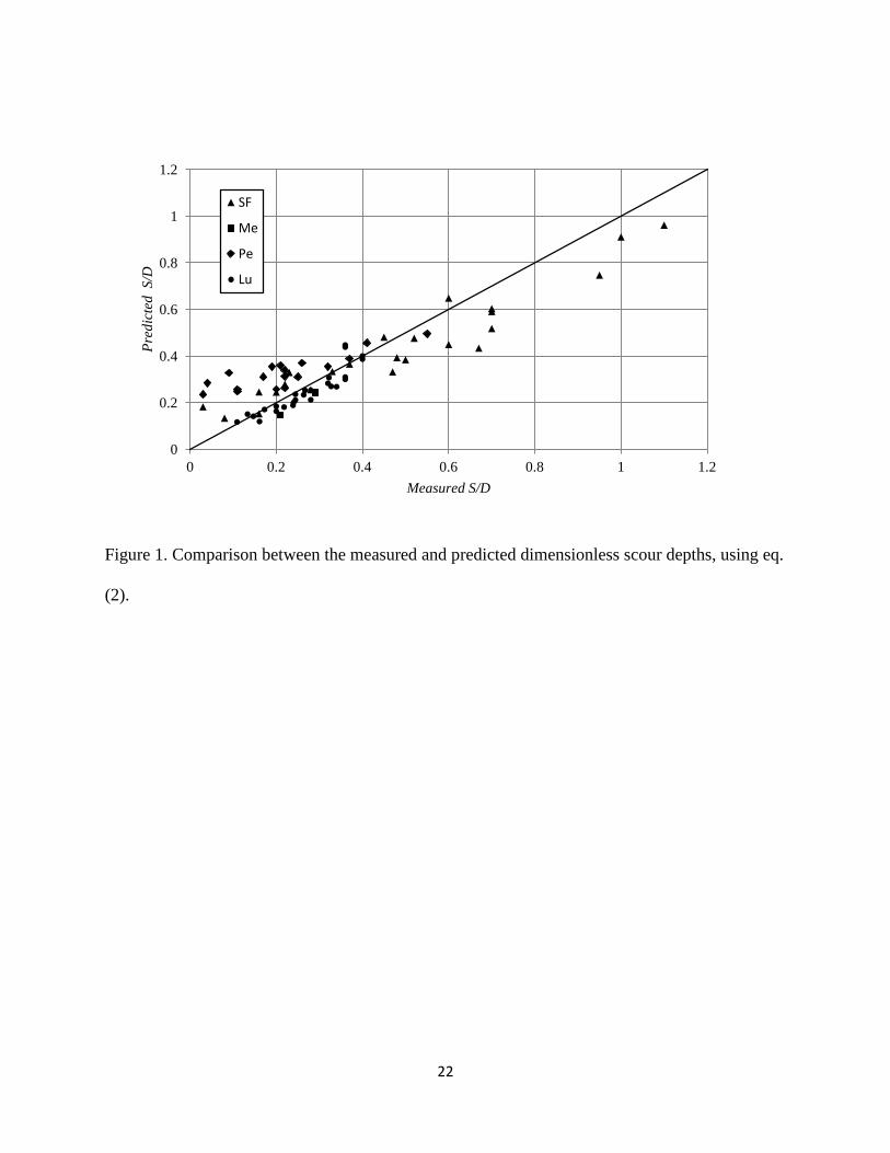
model is more accurate than the previous empirical equations. Hereafter, Lucassen [6], Sumer

and Fredsøe [7], Pu et al. [8] and Mousavi et al. [27] are referred to as Lu, SF, Pe and Me,

respectively. Figure 1 displays the comparison between the measured and predicted

dimensionless scour depth S/D, by eq. (2) for experimental datasets of Lu, SF, Pe and Me. As

7

seen, eq. (2) underestimates S/D for high values of S/D and overestimates it for low values of

S/D.

3. Model tree

Model trees generalize the concept of the classification and regression tree. They solve the

problem by dividing it into several sub-problem (sub-domain) tasks and the result is a

combination of these sub-problems. Classification trees classify data records by sorting them

down the tree from the root node to some leaf node. The difference between the better-known

classification trees and model trees is that the latter have a numeric value rather than a class label

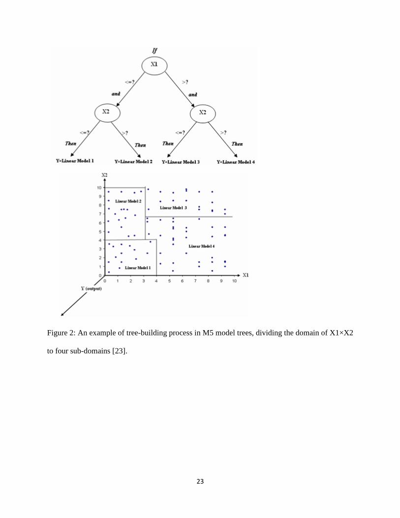
associated with the leaves. Model trees (MT) split the entire input or parameter domain into sub-

domains and a linear multivariable regression model is developed for each of them. Hence, they

can deal with continuous class problems and provide a structural representation of the data they

use piecewise linear models to approximate nonlinear relationships. Figure 2 displays the tree-

building procedure where the domain is divided to four sub-domains, each having a linear

regression model. According to the domain-splitting criterion, there are alternative algorithms to

build a model tree. One of the most popular algorithms is M5 algorithm [29]. In this algorithm,

first, the basic tree is build using the splitting criterion of standard deviation reduction (SDR)

factor:

( ) ( )∑ ×−=i

ii Esd

EE

EsdSDR (7)

where E is the set of examples (data records) that reach the node, Ei is the set that results from

splitting the node according to the chosen attribute (parameter) and sd is the standard deviation.

8

M5 uses standard deviation as an error measure of the class values that reach a node. By testing

all parameters at a node, it calculates expected reduction in error and then selects the parameter

that maximizes SDR. This process stops when the standard deviation reduction becomes less than

a certain percent of the standard deviation of the original dataset or when only a few data records

remain [29].

Then, a linear regression model is developed for each sub-domain. Only the data associated with

and the parameters tested in that sub-domain are used in the regression. Although the accuracy of

the tree model increases by growing the tree, over-fitting problem can occur during this process.

Pruning is used to avoid this by merging together a few lower sub-domains. The tree is pruned if

that results in a lower expected estimated error. Based on the Wang and Witten [30] approach,

the expected error is obtained by averaging the absolute difference between the predicted value

and the actual value for each of the training data points that reach that node. The expected error

can be underestimated outside the training data in this approach. For that reason, the expected

error is multiplied by (n+v)/(n-v), where n is the number of training data points that reach the

node and the v is the number of parameters in the model that represent the value at that node

[30].

After pruning, smoothing process is applied to compensate for sharp discontinuities occurring

between adjacent linear models at the leaves that improve the predictions [30]. As described by

Quinlan [29], in this process, the estimated value of the leaf model is filtered along the path back

to the root. The value at each node is combined with the value predicted by the linear model for

that node as P' = (np+kq) / (n+k) where P' is the prediction passed up to the next higher node, p

is the prediction passed to this node from the below, q is the value predicted by the model at this

node, n is the number of training data points that reach the node below, and k is a constant. Wang

9

and Witten [29] showed that smoothing substantially increases the accuracy of predictions. M5'

algorithm is a version of the M5 algorithm that has a similar structure to the M5. M5' algorithm

is able to deal effectively with missing values [29]. In this study, M5' algorithm in Weka

software [31] was used.

4. Description of the Datasets

In this study the experimental datasets of Lu, SF, Pe and Me were used. Lu’s experiments

were carried out in the wave flume with no initial gap between pipe and bed. The test conditions

in his experiments were as follows. Mean water depth: 50 or 25 (cm), mean sand size: 0.1, 0.22

and 0.7 (mm), pipe diameter: 2.5-18 (cm), orbital velocity: 10-25 (cm/s) and wave frequency:

0.25-1 (s). More detailed information can be found in Lucassen [5]. The SF experiments were

carried out in both wave flume and U-shaped tube. Their wave flume experiments were

conducted with four different pipe diameters (10, 20, 30, 50 mm). To study the effect of the

initial gap on the scour depth, some experiments were repeated with different initial gaps. In the

U-shaped tube, experiments were conducted with 30 (mm) diameter smooth pipe in different

initial gap. In the Pe’s experiments, a U-shaped oscillating water tunnel was used for both live

bed and clear water conditions. They used pipes with two diameters (2.89 and 1.91 cm) and

different initial gaps. Me’s experiments were conducted in a flume with different initial gaps.

They used smooth pipes with diameters of 11 and 6 cm. Most of the experiments were carried

out in the live bed condition ( crθθ > ). The critical Shields' number is calculated as [32]:

10

))02.0exp(1(055.024.0*

*

ddcr −−+=θ (8)

where, *d is dimensionless diameter of the bed sand:

31

250* ))((ρν

ρρ gdd s −= (9)

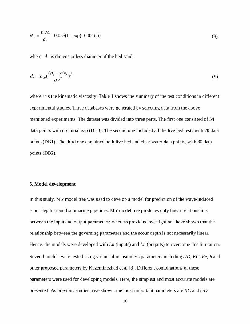
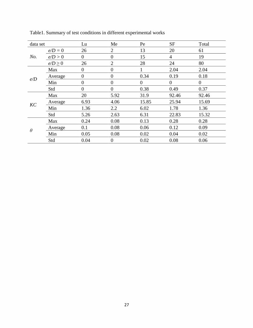
where ν is the kinematic viscosity. Table 1 shows the summary of the test conditions in different

experimental studies. Three databases were generated by selecting data from the above

mentioned experiments. The dataset was divided into three parts. The first one consisted of 54

data points with no initial gap (DB0). The second one included all the live bed tests with 70 data

points (DB1). The third one contained both live bed and clear water data points, with 80 data

points (DB2).

5. Model development

In this study, M5' model tree was used to develop a model for prediction of the wave-induced

scour depth around submarine pipelines. M5' model tree produces only linear relationships

between the input and output parameters; whereas previous investigations have shown that the

relationship between the governing parameters and the scour depth is not necessarily linear.

Hence, the models were developed with Ln (inputs) and Ln (outputs) to overcome this limitation.

Several models were tested using various dimensionless parameters including e/D, KC, Re, 𝜃 and

other proposed parameters by Kazeminezhad et al [8]. Different combinations of these

parameters were used for developing models. Here, the simplest and most accurate models are

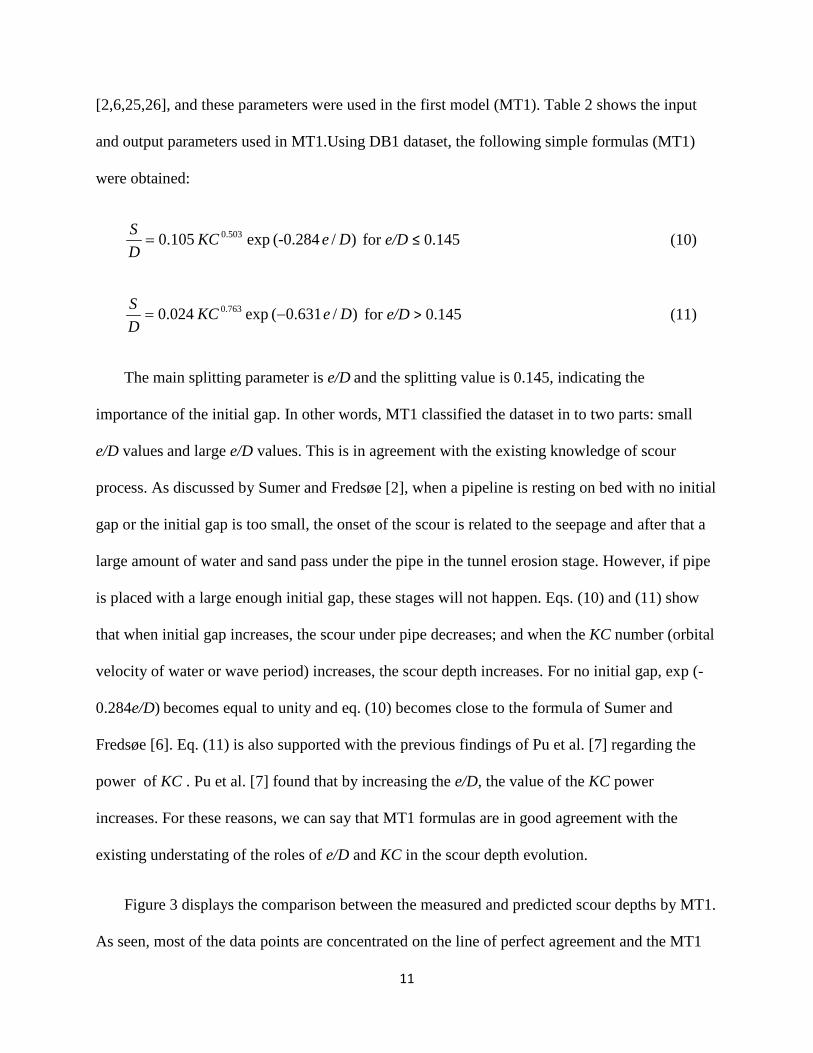
presented. As previous studies have shown, the most important parameters are KC and e/D

11

[2,6,25,26], and these parameters were used in the first model (MT1). Table 2 shows the input

and output parameters used in MT1.Using DB1 dataset, the following simple formulas (MT1)

were obtained:

)/ (-0.284 exp 0.105 0.503 DeKCDS

= for e/D ≤ 0.145 (10)

)/ 631.0( exp 0.024 0.763 DeKCDS

−= for e/D > 0.145 (11)

The main splitting parameter is e/D and the splitting value is 0.145, indicating the

importance of the initial gap. In other words, MT1 classified the dataset in to two parts: small

e/D values and large e/D values. This is in agreement with the existing knowledge of scour

process. As discussed by Sumer and Fredsøe [2], when a pipeline is resting on bed with no initial

gap or the initial gap is too small, the onset of the scour is related to the seepage and after that a

large amount of water and sand pass under the pipe in the tunnel erosion stage. However, if pipe

is placed with a large enough initial gap, these stages will not happen. Eqs. (10) and (11) show

that when initial gap increases, the scour under pipe decreases; and when the KC number (orbital

velocity of water or wave period) increases, the scour depth increases. For no initial gap, exp (-

0.284e/D) becomes equal to unity and eq. (10) becomes close to the formula of Sumer and

Fredsøe [6]. Eq. (11) is also supported with the previous findings of Pu et al. [7] regarding the

power of KC . Pu et al. [7] found that by increasing the e/D, the value of the KC power

increases. For these reasons, we can say that MT1 formulas are in good agreement with the

existing understating of the roles of e/D and KC in the scour depth evolution.

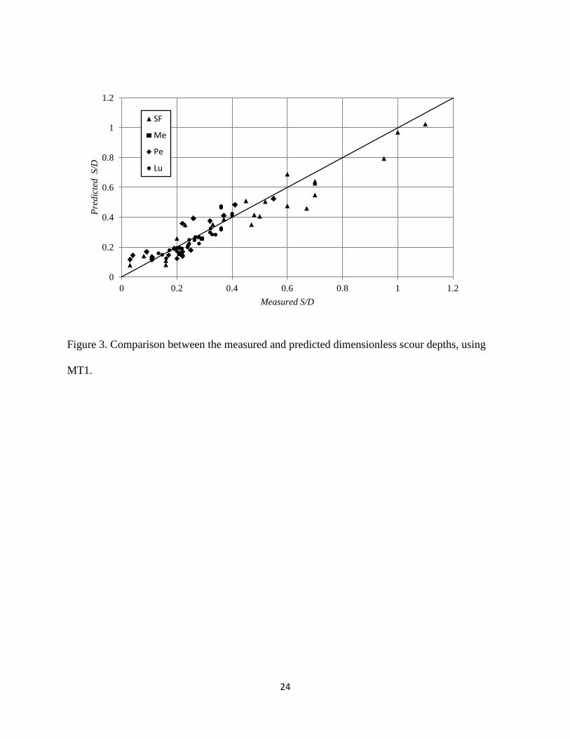
Figure 3 displays the comparison between the measured and predicted scour depths by MT1.

As seen, most of the data points are concentrated on the line of perfect agreement and the MT1

12

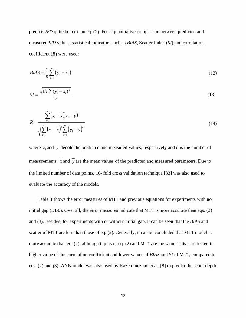
predicts S/D quite better than eq. (2). For a quantitative comparison between predicted and

measured S/D values, statistical indicators such as BIAS, Scatter Index (SI) and correlation

coefficient (R) were used:

( )∑=

−=n

iii xy

nBIAS

1

1 (12)

yxyn

SI ii2)(1 −∑

= (13)

( )( )

( ) ( )∑ ∑

∑

= =

=

−−

−−=

n

i

n

iii

n

iii

yyxx

yyxxR

1 1

22

1 (14)

where ix and iy denote the predicted and measured values, respectively and n is the number of

measurements. x and y are the mean values of the predicted and measured parameters. Due to

the limited number of data points, 10- fold cross validation technique [33] was also used to

evaluate the accuracy of the models.

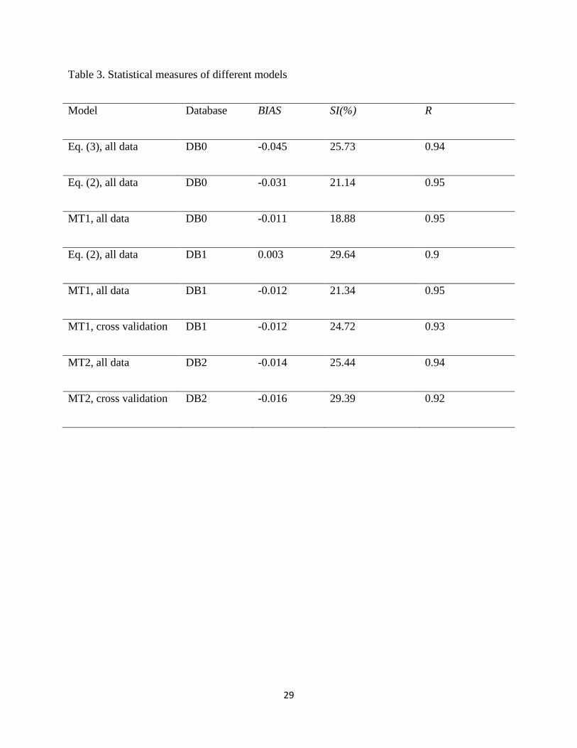
Table 3 shows the error measures of MT1 and previous equations for experiments with no

initial gap (DB0). Over all, the error measures indicate that MT1 is more accurate than eqs. (2)

and (3). Besides, for experiments with or without initial gap, it can be seen that the BIAS and

scatter of MT1 are less than those of eq. (2). Generally, it can be concluded that MT1 model is

more accurate than eq. (2), although inputs of eq. (2) and MT1 are the same. This is reflected in

higher value of the correlation coefficient and lower values of BIAS and SI of MT1, compared to

eqs. (2) and (3). ANN model was also used by Kazeminezhad et al. [8] to predict the scour depth

13

and the result were more accurate than eq. (2). However, the suggested model tree presents

simple mathematical formulas which are more transparent and easier to use.

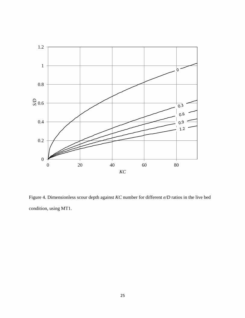
Figure (4) is given for better interpretation of eqs. (10) and (11). In this figure dimensionless

scour depth is drawn against KC number for different e/D ratios in the live bed condition. It

clearly shows that by increasing the e/D ratio the scour depth decreases and by increasing the KC

the scour depth increases. This figure can be used as a design diagram for engineers as well.

6. Extending the model for clear water condition

In order to investigate the clear water condition, DB2 data set was used and a new model

was developed for predicting the scour depth in both live bed and clear water conditions:

)/ 32.2exp( 344.3 296.1512.0 DeKCDS

−= θ for θ ≤ 0.064 (15)

)/ 472.0exp( 149.0 121.0477.0 DeKCDS

−= θ for θ > 0.064 and e/D ≤ 0.145 (16)

)/ 942.0exp( 048.0 121.0782.0 DeKCDS

−= θ for θ > 0.064 and e/D > 0.145 (17)

These formulas are consistent with existing understanding of the relative importance of the

parameters governing pipe scour depth. As discussed by Sumer and Fredsoe [2] the main

difference in live bed and clear water conditions is in the transport of the upstream sediments

which depends onθ . The main splitting value in MT2 is θ = 0.064. This shows that the MT2

classifies the dataset into two parts: θ < 0.064 that is close to clear water condition and θ > 0.064

that is close to live bed condition. The splitting value of the Shields parameter is close to the

14

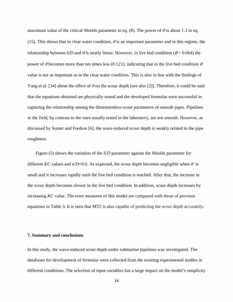
maximum value of the critical Shields parameter in eq. (8). The power of θ is about 1.3 in eq.

(15). This shows that in clear water condition, θ is an important parameter and in this regime, the

relationship between S/D and θ is nearly linear. However, in live bed condition (θ > 0.064) the

power of θ becomes more than ten times less (0.121); indicating that in the live bed condition θ

value is not as important as in the clear water condition. This is also in line with the findings of

Yang et al. [34] about the effect of θ on the scour depth (see also [2]). Therefore, it could be said

that the equations obtained are physically sound and the developed formulas were successful in

capturing the relationship among the dimensionless scour parameters of smooth pipes. Pipelines

in the field, by contrast to the ones usually tested in the laboratory, are not smooth. However, as

discussed by Sumer and Fredsoe [6], the wave-induced scour depth is weakly related to the pipe

roughness.

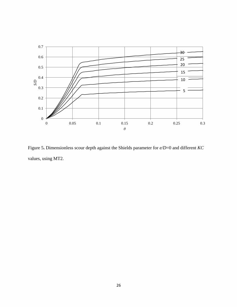
Figure (5) shows the variation of the S/D parameter against the Shields parameter for

different KC values and e/D=0.0. As expected, the scour depth becomes negligible when θ is

small and it increases rapidly until the live bed condition is reached. After that, the increase in

the scour depth becomes slower in the live bed condition. In addition, scour depth increases by

increasing KC value. The error measures of this model are compared with those of previous

equations in Table 3. It is seen that MT2 is also capable of predicting the scour depth accurately.

7. Summary and conclusions

In this study, the wave-induced scour depth under submarine pipelines was investigated. The

databases for development of formulas were collected from the existing experimental studies in

different conditions. The selection of input variables has a large impact on the model’s simplicity

15

and accuracy. Hence, based upon the previous studies, different dimensionless variables were

used for models development. M5' model, as a novel soft computing approach, was then used to

predict the dimensionless scour depth. Both live bed and clear water conditions were considered

and different dimensionless parameters were examined for developing the models. Two model

trees were developed to predict the scour depth. The used approach showed high performance for

all cases leading to the reduction of error statistics. The first one (MT1) was developed using KC

and e/D parameters for live bed conditions and its results were compared with those of previous

studies. It was found that MT1 model is physically sound and more accurate than the previous

empirical formulas. It was observed that in no initial gap condition, the MT1 model performance

was followed by the models of Sumer and Fredsoe [2] and Cevik and Yuksel [26] in terms of

accuracy. Then, another model (MT2) model was developed using KC, e/D and θ for both live

bed and clear water conditions. In both models, different equations were obtained for small and

large gap ratios, showing that the dependence of scour depth to KC and e/D is not monotonic.

The obtained formulas of MT2 showed a nearly linear relationship between dimensionless scour

depth and Shields parameter in the clear water condition and less dependency of S/D to the

Shields parameter in the live bed condition. The suggested formulas can be used easily by ocean

engineers and scientists for an accurate estimation of the wave-induced scour depth around

pipelines.

Acknowledgements

16

We are grateful to Ebrahim Jafari and Lisham Bonakdar for their constructive comments.

This study was partly supported by the Deputy of Research, Iran University of Science and

Technology (IUST).

17

References

[1]. Z.H. Zhao and H.J.S. Fernando, Numerical simulation of scour around pipelines using an

Euler-Euler coupled two-phase model. Environmental Fluid Mechanics, 7 (2007). 121-

142.

[2]. B.M. Sumer and J. Fredsoe, The mechanics of scour in the marine environment,World

Scientific, Singapor. 2002.

[3] C. Chen and J. Zhang, A review on scour modeling below pipelines, 2009, Proceedings of

Pipelines 2009: Infrastructures Hidden Assets, ASCE, 1019-1028

[4]. Y. Mao, The Interaction between a pipeline and an erodible bed, Institute of

Hydrodynamics and Hydraulic Engineering. Technical University of Denmark: Lyngby,

Denmark.1986.

[5]. B.M. Sumer, C. Truelsen, T. Sichmann and J. Fredsoe, Onset of scour below pipelines and

self-burial. Coastal Engineering, 42 (2001). 313-335.

[6]. R.J. Lucassen, Scour underneath submarine pipelines. MATs Rep. PL-4 2A, Marine Tech.

Res., The Netherlands. 1984.

[7]. B.M. Sumer and J. Fredsoe, Scour below pipelines in waves. Journal of Waterway Port

Coastal and Ocean Engineering, ASCE, 116 (1990). 307-323.

[8]. Q. Pu, K. Li and F.P. Gao, Scour of the seabed under a pipeline in oscillating flow. China

Ocean Engineering, 15 (2001). 129-137.

18

[9]. M.H. Kazeminezhad, A. Etemad-Shahidi and A.Y. Bakhtiary, An alternative approach for

investigation of the wave-induced scour around pipelines. Journal of Hydroinformatics,

12 (2010). 51-65.

[10]. D.F. Liang and L. Cheng, Numerical model for wave-induced scour below a submarine

pipeline. Journal of Waterway Port Coastal and Ocean Engineering, ASCE, 131 (2005).

193-202.

[11]. A.R. Kambekar and M.C. Deo, Estimation of pile group scour using neural networks.

Applied Ocean Research, 25 (2003). 225-234.

[12]. S.M. Bateni, S.M. Borghei and D.S. Jeng, Neural network and neuro-fuzzy assessments

for scour depth around bridge piers. Engineering Applications of Artificial Intelligence,

20 (2007). 401-414.

[13]. S.M. Bateni, D.S. Jeng and B.W. Melville, Bayesian neural networks for prediction of

equilibrium and time-dependent scour depth around bridge piers. Advances in

Engineering Software, 38 (2007). 102-111.

[14]. M.C. Deo, A. Jha, A.S. Chaphekar and K. Ravikant, Neural networks for wave

forecasting. Ocean Engineering, 28 (2001). 889-898.

[15]. M.H. Kazeminezhad, A. Etemad-Shahidi and S.J. Mousavi, Application of fuzzy

inference system in the prediction of wave parameters. Ocean Engineering, 32 (2005).

1709-1725.

[16]. Z.X. Zhang, C.W. Li, Y.Q. Qi and Y.S. Li, Incorporation of artificial neural networks and

data assimilation techniques into a third-generation wind-wave model for wave

forecasting. Journal of Hydroinformatics, 8 (2006). 65-76.

19

[17]. J. Mahjoobi, A. Etemad-Shahidi and M.H. Kazeminezhad, Hindcasting of wave

parameters using different soft computing methods. Applied Ocean Research, 30 (2008).

28-36.

[18]. B.G. Ruessink, Calibration of nearshore process models - application of a hybrid genetic

algorithm. Journal of Hydroinformatics, 7 (2005). 135-149.

[19]. K.W. Chau, A review on integration of artificial intelligence into water quality modelling.

Marine Pollution Bulletin, 52 (2006). 726-733.

[20]. L. Bonakdar and A. Etemad-Shahidi, Predicting wave run-up on rubble-mound structures

using M5 model tree. Ocean Enginering, (2010). under press

[21]. B. Bhattacharya, R.K. Price and D.P. Solomatine, Machine learning approach to modeling

sediment transport. Journal of Hydraulic Engineering, ASCE, 133 (2007). 440-450.

[22]. A. Etemad-Shahidi and L. Bonakdar, Design of rubble-mound breakwaters using M5 '

machine learning method. Applied Ocean Research, 31 (2009). 197-201.

[23]. A. Etemad-Shahidi and J. Mahjoobi, Comparison between M5 ' model tree and neural

networks for prediction of significant wave height in Lake Superior. Ocean Engineering,

36 (2009). 1175-1181.

[24]. S. Sakhare and M.C. Deo, Derivation of wave spectrum using data driven methods.

Marine Structures, 22 (2009). 594-609.

[25]. Y.M. Chiew, Mechanics of local scour around submarine pipelines. Journal of Hydraulic

Engineering, ASCE, 116 (1990). 515-529.

[26]. E. Cevik and Y. Yuksel, Scour under submarine pipelines in waves in shoaling conditions.

Journal of Waterway Port Coastal and Ocean Engineering, Asce, 125 (1999). 9-19.

20

[27]. M.E. Mousavi, A.Y. Bakhtiary and N. Enshaei, The Equivalent Depth of Wave-Induced

Scour Around Offshore Pipelines. Journal of Offshore Mechanics and Arctic

Engineering, Transactions of the ASME, 131 (2009).

[28]. J. Xu, G. Li, P. Dong, J. Shi, Bed form evolution around a submarine pipeline and its

effects on wave-induced forces under regular waves. Ocean Engineering, 37, (2010),

304-313.

[29]. J.R. Quinlan, Learning with continuous classes. 1992, Proceedings of AI'92 (Adams and

Sterling Eds), World Scientific. p. 343-348.

[30]. Y. Wang and I.H. Witten. Induction of model trees for predicting continuous

lasses.Proceedings of the Poster Papers of the European Conference on Machine

Learning. 1997. Prague: University of Economics, Faculty of Informatics and Statistics.

[31]. Weka, Waikato Environment for Knowledge Analysis software. 1999-2009, University of

Waikato: New Zealand.

[32]. R. Soulsby, Dynamics of Marine Sands: a Manual for Practical Applications, Thomad

Telford, London, 1997.

[33] I. H. Witten and E. Frank, Data Mining: Practical Machine Learning Tools and

Techniques, Morgan Kaufmann, San Francisco, CA. 2005.

[34]. B. Yang, F.P. Gao and Y.X. Wu, Experimental study on local scour of sandy seabed under

submarine pipeline in unidirectional currents. Gongcheng Lixue/Engineering Mechanics,

25 (2008). 206-210.

21

Figure captions

Figure 1. Comparison between the measured and predicted dimensionless scour depths using eq.

(2).

Figure 2: An example of tree-building process in M5 model trees, dividing the domain of

X1×X2 to four sub-domains [23].

Figure 3. Comparison between the measured and predicted dimensionless scour depths, using

MT1.

Figure 4. Dimensionless scour depth against KC number for different e/D ratios in the live bed

condition, using MT1.

Figure 5. Dimensionless scour depth against the Shields parameter for e/D=0 and different KC

values, using MT2.

22

Figure 1. Comparison between the measured and predicted dimensionless scour depths, using eq.

(2).

0

0.2

0.4

0.6

0.8

1

1.2

0 0.2 0.4 0.6 0.8 1 1.2

Pred

icte

d S

/D

Measured S/D

SF

Me

Pe

Lu

23

Figure 2: An example of tree-building process in M5 model trees, dividing the domain of X1×X2

to four sub-domains [23].

24

Figure 3. Comparison between the measured and predicted dimensionless scour depths, using

MT1.

0

0.2

0.4

0.6

0.8

1

1.2

0 0.2 0.4 0.6 0.8 1 1.2

Pred

icte

d S

/D

Measured S/D

SF

Me

Pe

Lu

25

Figure 4. Dimensionless scour depth against KC number for different e/D ratios in the live bed

condition, using MT1.

0

0.2

0.4

0.6

0.8

1

1.2

0 20 40 60 80

S/D

KC

26

Figure 5. Dimensionless scour depth against the Shields parameter for e/D=0 and different KC

values, using MT2.

0

0.1

0.2

0.3

0.4

0.5

0.6

0.7

0 0.05 0.1 0.15 0.2 0.25 0.3

S/D

θ

5

10

15

20 25

30

27

Table1. Summary of test conditions in different experimental works

data set Lu Me Pe SF Total

No. e/D = 0 26 2 13 20 61 e/D > 0 0 0 15 4 19 e/D ≥ 0 26 2 28 24 80

e/D

Max 0 0 1 2.04 2.04 Average 0 0 0.34 0.19 0.18 Min 0 0 0 0 0 Std 0 0 0.38 0.49 0.37

KC

Max 20 5.92 31.9 92.46 92.46 Average 6.93 4.06 15.85 25.94 15.69 Min 1.36 2.2 6.02 1.78 1.36 Std 5.26 2.63 6.31 22.83 15.32

θ

Max 0.24 0.08 0.13 0.28 0.28 Average 0.1 0.08 0.06 0.12 0.09 Min 0.05 0.08 0.02 0.04 0.02 Std 0.04 0 0.02 0.08 0.06

28

Table2. Input and output parameters of M5’ models

Model Input parameters Output parameter

MT1 Ln (KC), e/D Ln (S/D)

MT2 Ln (KC) , e/D , Ln(θ) Ln (S/D)

29

Table 3. Statistical measures of different models

Model Database BIAS SI(%) R

Eq. (3), all data DB0 -0.045 25.73 0.94

Eq. (2), all data DB0 -0.031 21.14 0.95

MT1, all data DB0 -0.011 18.88 0.95

Eq. (2), all data DB1 0.003 29.64 0.9

MT1, all data DB1 -0.012 21.34 0.95

MT1, cross validation DB1 -0.012 24.72 0.93

MT2, all data DB2 -0.014 25.44 0.94

MT2, cross validation DB2 -0.016 29.39 0.92