cesifo, a munich-based, globe-spanning economic research ... filevenice summer institute 2014 the...

Venice Summer Institute 2014

THE ECONOMICS AND “POLITICAL ECONOMY”

OF ENERGY SUBSIDIES

Organiser: Jon Strand

Workshop to be held on 21 – 22 July 2014 on the island of San Servolo in the Bay of Venice, Italy

CLEAN OR DIRTY ENERGY: EVIDENCE OF

CORRUPTION IN THE RENEWABLE ENERGY

SECTOR IN SOUTHERN ITALY

Caterina Gennaioli and Massimo Tavoni CESifo GmbH • Poschingerstr. 5 • 81679 Munich, Germany Tel.: +49 (0) 89 92 24 - 1410 • Fax: +49 (0) 89 92 24 - 1409

E-Mail: [email protected] • www.cesifo.org/venice

July 2014

CESifo, a Munich-based, globe-spanning economic research and policy advice institution

Venice Summer Institute

Clean or Dirty Energy: Evidence of Corruption in the Renewable Energy

Sector in Southern Italy.

Caterina Gennaioliú Massimo Tavoni †

Corresponding author: Caterina Gennaioli. Email Contact: [email protected], Address:

Grantham Research Institute on Climate Change and the Environment, London School of Eco-

nomics and Political Science. Tower 3, Clements Inn Passage, London WC2A 2AZ, UK. Telephone:

+4402071075433

úLondon School of Economics, Grantham Research Institute.†Fondazione Eni Enrico Mattei (FEEM) and Euro-Mediterranean Center on Climate Change (CMCC). Address:

Corso Magenta 63, Milan, Italy. Email: [email protected]

1

Abstract

This paper studies the link between public policy and corruption, for the caseof renewable wind energy. The insights of a model of political influence by interestgroups are tested empirically using a panel data of provinces in the South of Italyfor the period 1990-2007. We find significant evidence that: i) criminal associationactivity increased more in windy provinces, especially after the introduction of amore favorable policy regime and, ii) the expansion of the wind energy sectorhas been driven by both the wind level and the quality of political institutionsthrough their e�ect on criminal association. Our findings show that in the presenceof poor institutions, even well designed market-based policies can have an adverseimpact. The analysis is relevant for countries, which are characterized by heavybureacracies and weak institutions, like the South of Italy, and by large renewablepotential. JEL: D73, O13, H23. Keywords: Corruption, Government Subsidies,Natural Resources, Renewable Energy.

2

"If you [an energy company] are interested in investing in Calabria, I can reassure youthat it will be like a highway without toll gates" wiretapping of an ongoing judicial inquiryabout wind power. (Source: Corriere della Sera, October 25th 2012)

"Put up the money or no pole [for windmills] will be driven in the ground" wiretappingof a Mafia a�liate in Sicily in an ongoing judicial inquiry about wind power. (Source: LaRepubblica, June 10th 2013)

1 Introduction

The aim of this paper is to study and quantify the e�ect of public policy on corruption. Asan example of government intervention, we focus on the case of renewable energy. Renewableenergy provides an interesting and policy relevant case for a variety of reasons. The energysector is known to be both a target and a source of corruption, due to the characteristics ofthe energy resources, the possibility of generating rents, and the key oversight role playedby the government. For example, power generation and transmission as well as oil and gasare among the most bribery prone sectors, according to the Bribe Payers Index of Trans-parency International1. International organizations such as the World Bank, which havebeen involved in the financing of energy infrastructure in the developing world, have recog-nized the need to reduce corruption, often by trying to strengthen governance. As Mauro(1998) suggests, the need for secrecy characterizing the corrupt deals implies that “it will

be easier to collect substantial bribes on large infrastructure projects or highly sophisticated

defense equipment than on textbooks or teachers’ salaries”. Complicated regulations andpublic spending are among the major factors that can promote corruption (Tanzi (1998))and both elements characterize renewable energy projects.

Renewable energy is also extremely policy relevant. Renewable sources such as wind andsolar have been growing incredibly fast in recent years, especially in developed economiesand largely spurred by public support schemes aimed at promoting low carbon energy alter-natives. Developing regions like Africa host huge potential for renewables, which could beharvested in the near future to alleviate energy poverty and enable growth, two key com-

1http://bpi.transparency.org/bpi2011/

1

ponents of the U.N. Sustainable Energy For All initiative2. Moreover, policy instrumentsthat promote market flexibility in the regulation of greenhouse gases have incentivized thetrade of emission reduction credits between developed and developing countries (through theso-called Clean Development Mechanisms -CDM- of the Kyoto protocol). Renewable energynow represents the largest share of the CDM projects in the pipeline. Overall, renewableenergy provides an important case for testing whether public incentives fuel rent-seeekingand corruption in this sector.

Anecdotal evidence in Europe and elsewhere suggests the di�usion of corruption practicesrelated to public incentives for the renewable energy sector. Several o�cial inquiries madeby the Italian police have been made public, and have led to the arrest of managers andlocal politicians who allegedly used corrupt practices and bribes in order to obtain licenses tobuild wind farms. For example, according to a famous inquiry called “P3”, the entrepreneurFlavio Carboni and a former politician Pasquale Lombardi set up a criminal associationable to collect private funds from other entrepreneurs to pay bribes in exchange for windfarm permits in the region of Sardinia3. Similar scandals have occurred in Spain, where 19persons were arrested in 2009 with charges of corruption in the wind sector. In the U.S.,the bankruptcy of the solar power manufacturing firm Solyndra has led to a controversyover the potential influence of the Department of Energy on the loan guarantee the firm wasgranted. The aforementioned CDM schemes have been shown to not represent real emissionreductions, mostly as a result of perverse incentives and the quality of institutions (Victor(2011)). Many countries are now evaluating the public support policies which have beenimplemented over the past several years with the aim of promoting renewables. In mostcases, ex post policy assessment has focused on issues of e�ciency and e�ectiveness, buthas essentially disregarded the role of the main political economy factors at play. To ourknowledge, this is the first attempt to study whether public incentives to renewable energyresources could lead to an increase in illegal activities.

The main contribution of the paper is to understand whether the presence of a renewablenatural resource, such as wind energy, creates scope for rent seeking practices and corruptionwhen public incentives make it profitable to harvest the renewable potential. We do so byfirst presenting a model of political influence by interest groups, which yields predictions

2http://www.sustainableenergyforall.org/3http://www.repubblica.it/cronaca/2010/07/08/news/arrestato_flavio_carboni-5471098/

2

on the relation between corruption, renewable resources, and public support policies. Theseinsights are then tested on a panel dataset of provinces in the South of Italy for the period1990-2007. In the analysis we can exploit the presence of the renewable energy resource(e.g. wind potential) as inducing an exogenous variation in the expected rent opportunities.The empirical analysis provides strong evidence that supports our model, establishing thatthe expectations of high public incentives in the wind energy sector have fueled corruption,measured by the level of criminal association activity. Our main findings are that: i) criminalassociation activity increased more in high-wind provinces, especially after the introductionof a more favorable public policy regime and, ii) the expansion of the wind energy sector hasbeen driven by both the wind level and the quality of political institutions, through theire�ect on criminal association. In particular, comparing provinces with a similar (low) qualityof institutions, we find that the development of the wind sector has been higher in provinceswhere economic agents and bureaucrats have engaged more in criminal association activity,due to a high level of wind and of associated expected profits. The magnitude of the e�ectis significant: for an average wind park (of 10 MW) installed after 1999, and which receivesabout 1.5 Million euro per year in public support, the number of criminal association o�enseshas increased by 6% in the windy provinces with respect to the less windy ones.

Overall, the paper points out that even well designed market-based policies can have anadverse impact where institutions are poorly functioning. This e�ect would be greater inplaces with high resource potential. This has important normative implications especially forcountries, which are characterized by abundant renewable resources and weak institutions,and thus are more susceptible to the private exploitation of public incentives.

Related Literature The paper is related to the literature on corruption, which has shownhow highly regulated environments that render bureaucrats more powerful favor the spreadof corruption practices (Shleifer and Vishny (1993), Tanzi (1998))4. Several studies havefound that corruption is more detrimental to economic growth than taxation (Shleifer andVishny (1993), Fisman and Svensson (2006)), given the uncertainty and secrecy required bythe bribing process and the fact that corrupt deals cannot be enforced in courts. Moreover,corrupt o�cials might slow down the administrative process in order to collect more bribes

4Olken and Pande (2012), Sequeira (2012) and Svensson (2005) provide a comprehensive review of the literatureon corruption.

3

(Myrdal (1968), Kaufman and Wey (1998)). Although we cannot analyze the e�ect ofcorruption on the economic e�ciency of the renewable energy projects, we contribute to thisliterature by finding evidence of corruption in a heavily regulated sector and showing thatmore corrupt provinces have actually attracted a higher number of wind energy projects.

More specifically, a large literature has focused on the e�ect of public spending on po-litical and economic outcomes. Tanzi and Davoodi (1997) present cross country evidenceshowing a positive correlation between public investment and corruption. Hessami (2010)detects a positive relationship between the perceived level of corruption and the share ofspending on health and environmental protection. Finally, Lapatinas et al. (2011) developa theory to study the relationship between environmental policy and corruption. Using anoverlapping generation model with citizens and politicians, they show that corrupt politi-cians cause increased tax evasion which leads to a reduction of total public funds and thus,of environmental protection activities. Although suggestive, the evidence cannot establishthe direction of causality. At the micro level, Gennaioli and Onorato (2010) analyze the linkbetween public spending and organized crime activity in the Italian context, consideringreconstruction funds in the aftermath of the earthquake in the Umbria and Marche regionsas an exogenous increase in public expenditure. Using an instrumental variable approach,they find that an unexpected increase in capital expenses per capita raises the incidence ofthe number of Mafia-related crimes. In the authors’ view, organized crime acts as an en-trepreneur ready to move wherever economic opportunities arise, exploiting them to promoteillegal activity.

Our paper takes a di�erent perspective; the presence of the natural resource, when sup-ported by public policy, attracts criminal appetites and favors the formation of criminalassociations. However, the actual investments in the sector are not exogenous but driven bythe presence of a well established criminal association between entrepreneurs and politiciansable to influence the authorization process and thereby receive significant amounts of publicincentives. In this context, the level of wind capacity installed is expected to be determinedby the level of criminal association activity. A similar mechanism is described in a recentwork by Barone and Narciso (2011), showing that criminal organizations may distort the al-location of public investment subsides toward their areas of influence. Focusing on the e�ectof a raise in the expected rents from wind energy due to a government intervention, our study

4

is also related to a number of papers that have analyzed the impact of natural resource rentson corruption, political institutions and state stability (Bhattacharyya and Hodler (2010);Arezki and Bruckner (2011); Vincente (2010)). Vincente (2010) for example, analyzes thee�ects of an oil discovery announcement in the Island of Sao Tome and Principe. The authorfinds that the announcement increased the value of being in power for politicians and thisin turn created scope for resource misallocation, as vote-buying. Compared to Vincente,we are interested in the e�ects of a government intervention supporting renewables on thebehavior of economic and political agents, namely the entrepreneurs operating in the windenergy sector and the local bureaucrats who grant authorization permits. In this sense ourpaper is somewhat related to the literature on the e�ect of political connections (Fisman(2001), Fisman et al. (2012)), which studies how firms take advantage of being connected toa politician by circumventing regulation and securing permits, for example. To our knowl-edge, our paper is the first which is able to quantify the impact of renewable energy subsidieson corruption.

The paper proceeds as follows. In the next section we introduce a simple theoreticalframework which provides testable implications on the relationship between level of wind,corruption and the development of the wind sector. Section 3 describes the data and theinstitutional background. In Section 4 we outline the empirical strategy to test the model,and we present the empirical results. The final section concludes.

2 A Model of Corruption

The following model is linked to the broad literature on political influence by interest groupsand, in particular, it builds on the theoretical framework developed by Dal Bo et al. (2006).While in their model groups can influence policies both through bribes (plata) and threatof violence (plomo), we only consider bribes as a form of influence. Dal Bo et al. derivepredictions on the quality of public o�cials, while here we make predictions on the equilib-rium level of corruption and the number of active entrepreneurs as a function of windinessand institutional quality. Although the model is simple, it provides us with several testablehypotheses which we assess using empirical evidence for Italy.

The economy is divided in N administrative districts called provinces. Each province is

5

populated by a politician and an exogenously given number n of individuals, characterizedby a uniformly distributed ability parameter –, with U(0, 1). We consider a two stage game;in the first stage, individuals decide whether investing in wind power generation by buildinga wind farm, or carrying on their previous activity. If they do not invest in wind, they canearn a wage equal to their ability –. In order to invest, entrepreneurs in the wind energysector have to ask the politician for a permit. In the second stage, they decide whether topay the politician a bribe, b, so as to increase the probability of obtaining the permit. Inthis case the entrepreneur bears a cost of bribing, defined as ⁄Â(b). Â() is an increasingfunction of b and the parameter ⁄ captures institutional factors that might a�ect the cost ofpaying a bribe, such as the level of e�ort needed to keep corruption secret, which negativelydepends on the degree of social acceptance of bribing (it can also capture the quality oflaw enforcement, as suggested by Dal Bo et al.). In line with this interpretation, ⁄ can beinterpreted as a measure of the level of social capital.

The probability to obtain a permit in case of bribing is p, while in case of not bribingis q, with p > q. All other things being equal, if the politician receives a bribe, she willput more e�ort in the bureaucratic process, increasing the probability of the permit beinggranted. Once the entrepreneur obtains the permit, she can make the investment and builda wind farm. The return to investment is defined as I(w, F ), and depends on the revenuesassociated with the energy produced (increasing in wind w) on one side, and by the publicincentives on the other, F . The public support incentive can either remunerate the actualelectricity generated (for example through feed in tari� or a tradeable certificate system) orsubsidize the building of the wind farm (irrespective of how much it generates). In the firstcase, the introduction of a more favorable regime (increase in F ) leads to a higher Iw(), ’w.A regime switch from the second to the first support scheme would also make revenues moredependent on the wind level, and thus provide additional incentives to build in the windiestsites. The return to investment does not depend on the ability parameter since the windsector has traditionally been characterized by low levels of competition and revenues weremainly driven by public incentives.

In case of bribing, the entrepreneur gets away with probability c, while with probability(1 ≠ c) she is caught by the police and gets a payo� equal to zero. As in Dal Bo et al.,the utility of the politician linearly depends on money and on a moral cost, m, of being

6

corrupted. For simplicity, we normalize the politician’s wage to zero. Let the number ofavailable permits in each province be greater than n, such that entrepreneurs do not competefor permits; since we focus our attention on the first period after the introduction of windpower generation in Italy, we do not expect the limit in the number of permissions to bebinding. We solve the model for one province, so we can ignore index i in the notation. Thefollowing results can obviously be generalized for all provinces.

2.1 Equilibrium

We solve the model backward, starting from the second stage when an entrepreneur activein the wind energy sector has to decide whether to bribe the politician or not. Then we goback to the first stage, analyzing the entrepreneur’s decision to enter the renewable energysector. Following Dal Bo et al., we assume that the entrepreneur holds all the bargainingpower and makes a "take-it or leave-it" o�er to the politician.

2.1.1 Equilibrium Bribes

The politician accepts the bribe whenever the payo� under bribing is higher than the payo�without bribing, which is normalized to be equal to zero;

b ≠ m Ø 0 (1)

The entrepreneur chooses the level of the bribe, by solving the following problem:

Maxb

fi(b) © pc I(w, F ) ≠ ⁄Â(b)

s.t. b ≠ m Ø 0 (2)

Let bú denote the value of b that maximizes the profit of the entrepreneur under bribing, andfi(bú) be the optimal profit, with fi(bú) = pc I(w, F ) ≠ ⁄Â(bú). The entrepreneur, holdingall the bargaining power, will o�er the minimum bribe which makes the politician accept it.Let fi() © q I(w, F ), be the entrepreneur’s expected profit in case of not bribing. Then, theequilibrium bribe can be characterized as follows:

7

Proposition 1 An entrepreneur who decides to corrupt the politician o�ers a bribe bú =m. Therefore whenever fi(m) Ø fi(), we will observe bribing in the wind energy sector.

For any fi < fi, i.e. when the expected profit from bribing is lower than the one withoutbribing, the entrepreneur will not o�er the politician any bribe. Substituting for fi() andfi(), the bribing condition can be rewritten as:

I(w, F ) Ø ⁄Â(m)�POL

(3)

where �POL © (pc≠q) is defined as an inverse measure of the quality of political institutionsin a given province. �POL represents the di�erence in the probabilities of getting thepermit and not being caught; equivalently, it represents the net marginal return to bribingcompared to non-bribing option, in terms of probabilities. This measure captures the qualityof politicians or political institutions in general; the more a politician has been corruptedin the past, intervening in the bureaucratic process, the more she will be able to increasep compared to q, thanks to her connections and experience. Note that �POL can alsobe interpreted as a measure of the e�ciency of the bureaucratic process. Recalling theinterpretation of ⁄, the following definition is introduced.

Definition 1 Let

⁄Â(m)�POL

, be defined as a general index of the quality of institutions

(QI), where the numerator refers to its social dimension (i.e. social capital), while the

denominator measures its political component.QI denotes the threshold level for the expected revenues in the wind sector, such that the

entrepreneur is indi�erent between bribing and not bribing. Note that QI can be interpretedas an inverse measure of the extent of corruption or the likelihood to observe bribing, since itrepresents the set of possible values for which bribing is not profitable for the entrepreneur.Intuitively, the lower the general quality of institutions in a certain province is, the morelikely it is to observe corrupted deals; if QI is su�ciently low, the net marginal return tobribing increases and, as a consequence, the incentive to bribe rises for entrepreneurs activein the wind energy sector. Summing up, taking into account both the political and the socialdimension of the QI index, active entrepreneurs have more incentive to bribe the politiciansin provinces where political institutions are badly functioning and bribing is socially tolerated(lower social capital), such that less e�ort is required to keep illegal deals secret.

8

2.1.2 Entry Decision

Turning to the first stage, we analyze the entry decision. An entrepreneur will decide to enterif the expected return to wind energy investment is higher than her reservation wage, whichis equal to her ability type. Let us focus on non-trivial solutions, studying the case where�POL > 0. Taking into account the condition for bribing, the equilibrium is characterized,distinguishing between two cases:

Lemma 1 (a) If I(w, F ) 1 QI; all entrepreneurs with ability type – 0 pc I(w, F ) ≠

⁄Â(m), enter the wind energy market and choose the bribing option. (b) If I(w, F ) < QI;all ability types with – 0 q I(w, F ), enter the wind energy market and do not bribe.

According to the model, two contrasting types of markets for wind energy can emerge inequilibrium; one in which all agents are corrupted, and the other where all agents behavehonestly. First notice that, in both types of markets, the ability type of active entrepreneursis increasing in the expected revenues of wind investment; as long as the return to investmentdoes not increase much compared to the one in the non-wind sector, only the lower abilitytype will enter the renewable energy market. These low types would anyway achieve higherprofits in the wind sector, thanks to the amount of public incentives. Whether a provincewill experience a corrupted wind market or not depends both on QI and the wind level.The equilibrium outcome, described in Lemma (1), is intuitive; the level of wind, a�ectingthe returns to investment, leads economic agents to enter the wind energy market. Whetherthis is correlated with an increase in bribing practices depends on institutional quality; ifthe politician’s intervention significantly increases the probability to obtain the permissionand corruption is generally tolerated in the society, high wind is correlated with a highernumber of corrupted agents active in the wind energy market; if instead, without the directintervention of the politician, the entrepreneur faces almost the same probability to get apermit and corruption is viewed poorly in the society, then a high wind level is correlatedwith a higher number of honest agents active in the market. From now onwards, we focuson the emergence of the corrupted type of market and study some related comparativestatics. Since in the empirical part only the Southern regions of Italy will be considered,it is reasonable to assume that all provinces in our sample satisfy condition (a), due to asimilar, and relatively low, quality of institutions. Let corr be the extent of corruption in aprovince (belonging to group (a)); since, according to the previous lemma, all entrepreneurs

9

entering the wind sector bribe the politician, we define the level of corruption as the numberof entrepreneurs active in the market.

Definition 2 Given lemma (1), the equilibrium level of corruption in a province belonging

to group (a), can be defined as:

corrú = F [pc I(w, F ) ≠ ⁄Â(m)] (4)

where F is the pdf of –. Given the assumption on –’s distribution, we can simply rewrite(4) as:

corrú = pc I(w, F ) ≠ ⁄Â(m) (5)

Consistent with the intuition provided above, corruption in this equilibrium depends bothon the level of wind and the quality of institutions. In other words, taking the wind level asconstant, one should observe a higher level of corruption in provinces with worse institutionalquality, in both its social and political dimensions.

2.1.3 Comparative Statics

Some interesting comparative statics can be derived, in terms of wind level and the type ofpolicy in place.

Lemma 2 The equilibrium level of corruption is increasing both in the wind level and in

pc, which is inversely related to the quality of political institutions. Formally:

ˆcorrú

ˆw= pc Iw (w, F ) ,

ˆcorrú

ˆ (pc) = I(w, F ), (6)

ˆcorrú

ˆwˆpc= ˆcorrú

ˆpcˆw= Iw 1 0 (7)

Condition 7 shows the complementarity between windiness and the quality of political insti-tutions, in determining the equilibrium level of corruption; considering two provinces withthe same wind level but with a di�erent probability of obtaining the permit via bribing,one should expect a higher level of corruption in the province with worse political institu-tions. On the other hand, comparing two provinces with similar chances of using bribes toget permits, but a di�erent level of wind, one should expect more corruption in the high-wind province. The intuition behind these results is simple; since the marginal return to

10

bribing is increasing in the wind level, we should expect a higher number of entrepreneursentering in high-wind provinces and bribing the politician. The negative e�ect of windinesswill be stronger in provinces characterized by a lower political quality. In the same way, alower quality of political institutions increases the number of corrupted entrepreneurs in themarket, and it does so more in high-wind provinces that entail a larger margin of profit.

The next result provides interesting policy implications for the Italian case and elsewhere.In principle, a policy promoting renewables can be designed in two ways: i) increase thesubsidy to build the wind farm, through a lump sum transfer as development funds (F1)or, ii) increase the remuneration of the policy based on the actual production, in our caseproxied by wind level, which can be interpreted as the introduction of a market-based typeof policy such as a feed in tari� or a tradeable certificate system (F2).

Lemma 3 Both an increase in the lump sum transfer and in the remuneration of the

electricity generated increase the extent of corruption, with: a)

ˆcorrú

ˆF1= pc and b)

ˆcorrú

ˆF2=

w pc.If one looks at second order e�ects, the lemma generates an important result, pointing

out a di�erent impact of the two types of policy on the level of corruption. In particular,while an increase in the lump sum equally raises the level of corruption in all provinces withsimilar probabilities of getting the permit through bribing, the introduction of the market-

based system leads to a greater increase in corruption in provinces characterized by a higherwind level. The logic is the same as before; in general, higher amounts of public incentivesincrease the return to wind investments, and lead a larger number of agents to enter themarket. However, if the quality of political institutions is low (as in the region analyzed inthe empirical section), all the entrants opt for the bribing option and, as a consequence, thenumber of entrepreneurs involved in bribing becomes larger. Moreover, if the public incentivebecomes more responsive to the actual energy generated (i.e. to the wind level), this e�ectbecomes stronger in high wind provinces. This result shows that in the presence of poorlyfunctioning institutions, a market based policy might actually have a larger negative impact,particularly where the greatest e�ciency gains could be obtained, namely in provinces withthe highest energy potential.

After having derived conditions on the entry and bribing decision of the entrepreneurs,we finally characterize the wind energy sector, analyzing the expected amount of investments

11

in each province. Also in this stage, we focus on provinces belonging to group (a) in Lemma1.

Definition 3 The expected number of projects, E(P ), in a certain province, is defined as

the total number of active entrepreneurs in the market, weighted by the probability to get the

permit. In particular:

E(P ) = pc

ˆ –

0f(–)d– (8)

Given that – © pc I(w, F ) ≠ ⁄Â(m) and f(–) = 1, and using the definition of corruption,we obtain that::

E(P ) = pc [corr] (9)

Expression 9 points out that the expansion of the wind energy sector is a positive linearfunction of the level of corruption. In other words, marginal returns to corruption, in termsof authorized wind plants and installed capacity, are positive and constant. Recalling thecomplementarity between the wind level and the political institutions quality in determiningthe level of corruption, the following result can be derived.

Proposition 2 The expected number of wind energy projects in a certain province posi-

tively depends on its level of corruption. In particular, i) given two provinces with the same

wind level, the expected number of wind energy projects will be higher in the province with

worse political institutions, and, ii) given two provinces with the same (low) quality of po-

litical institutions, the expansion of the wind energy sector will be greater in the windiest

province.

As we have seen before, an increase in the returns to bribing (due to a change in thewind level, the policies or the quality of political institutions), leads a higher number ofentrepreneurs to enter the wind energy sector and bribe the politicians. The level of corrup-tion in equilibrium will be higher and, as a consequence, the actual number of wind projectsput in place will increase as well. Considering provinces where the quality of institutions issu�ciently low and chances of obtaining permits with bribes are high, this section highlightsthat not only the wind level but also the quality of institutions are crucial determinants ofthe development of the wind energy sector, through their e�ect on corruption. This is dueto the fact that in our model, corruption helps to cut the red tape, eventually accelerating

12

the development of the wind sector. Though in principle corruption can also hamper thedevelopment of an industry by imposing additional and unnecessary costs, the evidence ac-cumulated in the o�cial inquiries is consistent with the first hypothesis, especially given thesignificant size of the public subsidies in the wind sector (see Section 3.1).

2.2 Discussion

Using a simple model of corruption we have analyzed the main factors which can fuel bribingin the emerging market of wind energy. Given the data available, we cannot test all the modelpredictions and we will mainly focus on the role of the wind level in determining corruptionand wind plant installations. Nonetheless, having data covering a su�ciently long timeperiod, we can analyze the e�ects of the transition between the two major policy regimesimplemented to promote wind energy. The main predictions of the theory which we take tothe data are the following:

i) Ceteris paribus, the windiest provinces are more likely to experience corruption.ii) The increase in the remuneration of wind investments, due to the introduction of a

market-based policy regime, leads to an increase in the extent of corruption, especially inhigh-wind provinces.

iii) The number of wind energy projects in a given province increases with the extent ofcorruption.

As we have seen, the expansion of the wind energy sector is not only driven by thelevel of wind but also by the functioning of social and political institutions. This suggeststhat, comparing provinces with the same wind level, the number of wind projects shouldbe higher in provinces where a larger number of agents have been involved in corruptionpractices, due to a poor quality of institutions. Among provinces with a similar (low) qualityof institutions, the expansion of the wind sector should be greater in places where criminalassociation activity is more frequent due to a high level of wind and the associated expectedrevenues.

13

3 Background and Data

3.1 Wind Power in Italy

The incentives schemes to renewables, including wind power, began in 1992, when a feed-intari� known as CIP 6 was introduced to support renewables and "assimilated sources"5. Thefeed-in tari� system managed to jump start investments which were important at a time ofshortage of available power capacity, but also uncovered several flaws.

In order to overcome these pitfalls, and following the liberalization of the Italian electricitymarket, in 1999 a market-oriented mechanism based on tradable green certificates (knownas “Certificati Verdi”, CV) was implemented; this required power producers and importersto have a minimum share of electricity generated by renewable sources. The quota was setfor the initial date of operation in 2001 at 2%, gradually increasing over time (it is now7% ). Green certificates can be exchanged on either the Italian electricity market or viabilateral contracts, and last for several years (12 and 15 years if issued before and after2007 respectively). In the initial phase, an excess of demand pushed the prices of the greencertificates up, above 100Euro/MWh (see Table 1). This induced a sizable increase in thesupply of renewable power, mostly wind, hydro and biomass, so that supply started exceedingthe allocated quotas from 2006. In order to prevent prices from dropping too low, in 2008 thegovernment intervened and e�ectively turned the quota system back into a feed-in tari� one.In addition to the CV incentives, revenues also accrue for electricity generation, thanks topriority dispatch to the electricity market or alternatively to the option of selling electricityat a minimum guaranteed price.

5The terminology has allowed several other sources, including thermal co-generation, to be included among thebeneficiaries of the feed-in tari�, which has undermined the e�ectiveness of the policy in promoting traditionallyrenewable energy. Though the exclusion of ‘assimilated’ sources from the incentives has been mandated in theEuropean directive 2001/77/CE, a series of waivers have allowed this practice to persist to date.

14

Table 1. Green certificate market (source: GME and AEEG)

tari� known as CIP 6 was introduced to support renewables and "assimilated sources"5. Thefeed-in tari� system managed to jump start investments which were important at a time ofshortage of available power capacity, but also uncovered several flaws.

In order to overcome these pitfalls, and following the liberalization of the Italian electricitymarket, in 1999 a market-oriented mechanism based on tradable green certificates (knownas ‘Certificati Verdi’, CV) was implemented; this required power producers and importersto have a minimum share of electricity generated by renewable sources. The quota was setfor the initial date of operation in 2001 at 2%, gradually increasing over time (it is now7% ). Green certificates can be exchanged on either the Italian electricity market or viabilateral contracts, and last for several years (12 and 15 years if issued before and after2007 respectively). In the initial phase, an excess of demand pushed the prices of the greencertificates up, above 100Euro/MWh (see Table A). This induced a sizable increase in thesupply of renewable power, mostly wind, hydro and biomass, so that supply started exceedingthe allocated quotas from 2006. In order to prevent prices from dropping too low, in 2008 thegovernment intervened and e�ectively turned the quota system back into a feed-in tari� one.In addition to the CV incentives, revenues also accrue for electricity generation, thanks topriority dispatch to the electricity market or alternatively to the option of selling electricityat a minimum guaranteed price.

average price (Euro/MWh) overall cost (M Euros)

2003 98.9 243

2004 116.8 263

2005 130.9 332

2006 142.8 488

2007 99.0 306

2008 103.6 400

Table A: Green certificate market (source: GME and AEEG)

The financial incentive regime for investment in renewables in Italy appears to be advan-tageous by international standards. The Italian energy authority has estimated the cost of

5The terminology has allowed several other sources, including thermal co-generation, to be included among thebeneficiaries of the feed-in tari�, which has undermined the e�ectiveness of the policy in promoting traditionallyrenewable energy. Though the exclusion of ‘assimilated’ sources from the incentives has been mandated in theEuropean directive 2001/77/CE, a series of waivers have allowed this practice to resist to date.

14

The financial incentive regime for investment in renewables in Italy appears to be advan-tageous by international standards. The Italian energy authority has estimated the cost ofthe green certificate trade system at 400 million Euros in 2008, with the prospect of passingto 1 billion in 2013. In addition, regional and provincial support schemes have also been putinto place. The contribution of wind power has increased significantly after the introductionof the CV incentive system, and now contributes to almost 4% of of the national electricityconsumption. Virtually all the installed wind capacity is concentrated in the “Mezzogiorno”,which hosts the largest wind potential (see Figure 1 below).

Figure 1. Map of wind resources in Italy (speed at 75m height, source CESI)

39

Figure 1. Map of wind resources in Italy (speed at 75m height, source CESI)

Figure 2. Distribution of wind installed capacity by province at the end of 2011 (source GSE)

15

The provinces of Foggia (FG), Benevento (BN) and Avellino (AV), which lie on the windyridge of the south Appennines, host roughly one third of the whole national capacity. Thesesites, together with the ones in Sardinia, were also the first to develop, and are characterizedby higher utilization factors. More recently wind power has considerably expanded to severalprovinces of Sicily and Calabria.

Within the provinces, these rents are concentrated in a subset of municipalities, oftenof small size and located in areas with low population density. Thus, the royalties thatthe wind parks can yield to the local authorities (either legally or illicitly) -in exchange forthe construction authorization- can be considerable, enough to induce corruption practices.Until 2010, there were no o�cial guidelines on the rules for determining such royalties, andthese were left to the discretion of local authorities, without any national harmonization. Inaddition, region-wide energy plans have been introduced quite slowly, allowing for a quiteunregulated environment, which for example has only been partially able to account forother factors such as the integration with the electricity grids. Though the magnitude ofthe incentives is large, it is important to note that the wind sector still represents a smallfraction of the overall economic output. The share of wind profits over the total value addedof the economy does not exceed 2%, even in the most favourable provinces to wind.

For the sake of our analysis, we assume that the regime change that the green certificatesystem brought about in 1999 (with e�ective use from 2001) can be considered the real turn-ing point for policy. In the language of our model, this policy break has increased the returnto wind investment I(w, F ), and thus motivated more illicit activities. Although, as we haveseen in this section, policies supporting renewables were present in the country even beforethe turn of the century, there are various reasons to support the idea that the green certificatesystem represented a significant policy regime switch. First, the commitment to renewablesof the European Union strengthened markedly around that time, culminating in the RES(Renewable Energy Support) directive which took e�ect in 2001 and set national indicativetargets for renewable energy production from individual member states for the years 2010and 2020. This increased the certainty of the policy support schemes for renewables, alsoproviding a long term perspective in terms of quotas. Second, the liberalization of the Italianelectricity market and the increased dynamics of the international energy markets, with oilprices starting to rise in 1999 and especially after 2001, provided an increased opportunity

16

to enter a sector which was traditionally monopolistic. Finally, the wind turbine technologyimproved dramatically over time: the investment costs dropped considerably, from roughly2000 to 1000 US$/kW. The reliability of the technology also increased, as it became bettersuited to handle times of strong winds. Thus, the green certificate (CV) system marked aclear change in terms of public support to the deployment of wind power, as testified by themarked increase in installed capacity post 2000 (see Figure 5).

The questions of interest for us are, a) whether in general, there is a positive correlationbetween the development of the wind energy sector and corruption and, b) if corruptionpractices, fueled by the expectation of huge profits (mostly due to public incentives), arepartly responsible for the large expansion of the sector.

3.2 Data Description

We use a panel dataset for the period 1990-2007 with annual observations on 34 provincesof Southern Italian regions6. We make use of a data set compiled by the Italian NationalInstitute of Statistics (ISTAT, “Statistiche Giudiziarie Penali”) to measure criminal activityin the country. To compute the extent of corruption we use two measures: a) criminalassociation activity (CrimAssoc), representing the number of “Criminal Association” o�ensesbrought to justice by the five sectors of the police force, and b) total criminal association(TCrimAssoc), the sum of o�enses related to “Criminal Association” and “Mafia-relatedCriminal Association”. Values are reported in terms of incidence per 100,000 inhabitants.Criminal association activity represents a very good measure of the level of corruption in thewind energy sector since, according to the Italian penal code, “it implies a su�ciently stableorganization of two or more individuals who agree on committing illegal activities”. This isexactly the case of the local bureaucrat which systematically exchanges authorizations forbuilding wind farms for bribes from entrepreneurs. Actually most of the persons involved incorruption activity in the wind energy sector have been charged with this type of o�ence7.As a robustness check, we make use of a third and somewhat unrelated measure of criminalactivity, the index of violent crime.

6For sake of comparison, Italian provinces are similar in size to US counties. During the period analyzed, sevennew provinces were instituted in the South of Italy. We disregard changes to the 1990 province classification, andattribute data on new provinces to those they originated from.

7See the example reported in the Introduction.

17

The set of controls includes the log of real GDP per capita and the secondary schoolenrollment at the provincial level as provided by ISTAT. These controls are widely used inthe crime literature and represent potential determinants of criminal behavior measuring theexpected earning and cost opportunities. In order to control for the impact of populationdensity on the level of criminal association, we conform to Bianchi et al. (2012) and includethe log of the resident population in the province among our controls. Finally we also includethe index of violent crime as a control to account for criminal attitudes in a given province.This is computed on the basis of the o�enses brought to justice by the five sectors of thepolice force regarding the following crimes: massacre, homicides, infanticide, lesions, sexualassaults, kidnapping, assassination attempts and theft.

The expected number of projects, E(P ), is proxied by the number of wind plants and thetotal capacity installed; for this purpose, since o�cial statistics at the provincial level are onlyavailable from 2008 onwards, we rely on a dataset compiled by ANEV (National Associationfor Wind Energy). This covers the totality of wind parks, and provides data on the location,capacity, size, year of initial operation, and ownership. Wind level, w, is computed usingdata coming from the Italian Wind Atlas , which provides the average wind level (at di�erentdistances above sea level) per square kilometer for the whole Italian territory. In order toassign each province to a certain class of wind, we construct our own measure of windiness.In particular, we classify provinces according to their wind level8, taking into account thesize of the province; considering the quartiles of the wind distribution, we divide the windmeasure in four classes, then we compute the fraction of total provincial area lying abovethe third quartile, or 5.2 m/s (meters per second). For example the 8 windiest provinces arethe ones with more than 25% of their area above the third quartile of wind distribution, thefollowing 9 windiest provinces have between 17% and 25% of their area lying above the thirdquartile of wind distribution, and so on. The level of windiness we assign to each provicecorresponds to the quota of the provincial area lying above 5.2 m/s multiplied by the averagewindiness above the same threshold. The figure below reports the distribution of the WindIndex across all the provinces in the sample.

8Wind speed is computed at 25 meters above the sea level

18

Figure 2. Distribution of the Wind Index

40


TABLE B. Descriptive Statistics

Variables Mean CrimAssoc 2.277

(1.775) TCrimAssoc 3.034

(2.342) Violent crime Index 115.018

(72.496) Clear_Up (N. Obs.=476)

0.332 (0.115)

Wind_Index 1.227 (0.95)

Wind Plants 2.236 (4.848)

Capacity (MW) 18.123 (54.356)

GDP_pc 9.490 (0.184)

School

0.814 (0.12)

Population 609323 (544902.4)

N. Obs. 612 Standard deviations in parentheses.

3.3 Measurement Issues

A well known issue in crime-related literature regards the problem of using counts of reportedcrimes. This can lead the underestimation of the true number of committed crimes and biasthe estimates if the explanatory variables of interest are correlated with the level of under-reporting. In our case, the bias in reporting originates from the police investigative activity:criminal association is a di�cult crime to detect as most times it does not involve a directvictim with the interest to report to the police. Rather, it is usually the police that reportthis type of o�ence to the judiciary after an investigation process. In this analysis our majorconcern is to measure criminal association levels rather than the extent of investigationactivity by the police. Ehrlich (1996) extensively discussed the reporting bias in crime dataand proposed several remedies9. We use one of them, recently adopted by Fougere et al.(2009) and Bianchi et al. (2012), which consists in exploiting the panel structure of thedata including time and province fixed e�ects. This method is very e�ective since it takesinto account any systematic di�erence in police reporting activity between provinces (overtime) or between di�erent times (across provinces). We also include province specific timetrends which allows for time varying, province specific bias in crime reporting by the police.

9See also Levitt (1996), Fougere et al (2009), Gould et al. (2002)

19

Finally, we further address this issue using a measure for the e�ciency of police activity,namely the clear-up rate, defined as the ratio of crimes cleared up by the police over thetotal number of reported crimes. Since the data are only available until 2003 we just presentsome descriptive statistics.

4 Methodology and Results

The main hypothesis we want to test is whether the presence of a renewable natural resource,namely wind energy, can favor the spread of corruption practices, especially in the presenceof public policies like subsidies. A related question is whether the increase in the expectedreturns of investments in wind energy drive economic agents to increasingly engage in rent-seeking activities. As we have seen, profits in the wind energy sector started to increase afterthe introduction of the green certificate (CV) system, when a significant amount of publicincentives were granted; thus, we would expect an increase in corruption especially after thatperiod. But what are the e�ects of this increase in corruption on the actual expansion of thewind energy sector? To answer this question, in the last part of the empirical exercise wetest the third prediction of our analytical model, namely the positive association betweenthe degree of corruption and the actual expansion of the wind sector. Summing up, thecausation chain we have in mind and are going to test is the following:

Wind Intensityæ Criminal Association Activity (Corruption)æ Wind Capacity InstalledWe start analyzing the first link, and explore the second one in the last part of this

section.Empirically addressing this set of issues is di�cult since there may be confounding fac-

tors a�ecting the level of criminal association activity. As we have seen, the model givesthe wind level and the quality of institutions a central role in determining the extent ofcorruption. We exploit the exogenous variation in wind level across provinces to addressour estimation in a robust way. First, considering all the provinces in our sample, we checkwhether the wind level is positively associated with the level of criminal association activity,especially after the policy break of 1999-2001. To further investigate this relationship, wethen focus on the 8 windiest provinces10 which represent the top quartile of our measure (i.e.

10AV, BN, CA, CZ, FG, PZ, SS, TP

20

provinces with more than 25% of their area lying above the 5.2 m/s threshold). Employ-ing a di�erence-in-di�erence strategy, we compare the windiest provinces in the area of theSouth of Italy (treatment group) to all other provinces in the sample (control group). Thisapproach, however, implies a comparison between two highly heterogeneous groups. In orderto consider two similar groups we refine the analysis comparing the 8 windiest provinces tothe 11 neighboring provinces. Through the analysis we divide the time span into severaltime windows, focusing on subperiods due to the dynamics of returns to wind energy, ourcorruption-inducing variable. Specifically, returns to wind energy experienced a significantincrease after 1999.

As mentioned above, in order to identify the windiest provinces we use a very accuratedatabase to construct a measure of average windiness that takes into account the fractionof total provincial area lying above the third quartile of the wind resource distribution. Thechoice of the treatment group in the di�erence-in-di�erence exercise is not an obvious one,since the wind threshold can be set at di�erent levels. However, as already noted, there isa handful of provinces that by far hosts the greatest wind potential, and only very recentlythis has begun to expand to other ones. In addition, since our analysis stops in 2007, therestricted group of 8 provinces is the most meaningful group to look at. We do not have datato measure the quality of institutions, but since this can be considered a persistent element,we partly solve the omitted variable problem using province fixed e�ects.

4.1 Evidence on Criminal Association

We begin our empirical investigation by testing the model predictions i) and ii), namelywhether windier provinces are more likely to experience corruption, and whether the intro-duction of a new policy regime further increased corruption in windy provinces. In order toassess the relation between wind and criminal association activity over time for all the 34provinces in the sample, we first estimate the following equation (a):

CrimAssoci,t =ÿ

–t≠t+3tœT

Windi,t≠t+3 + xi,t” + “itrendi,t + ui + vt + Ái,t (a)

Where CrimAssoci,t measures the number of charges made by police forces for criminalassociation o�enses in province i at time t, Windi,t≠t+3 is equal to the wind level (as measuredby our wind index) in province i between time t and t+3, and zero otherwise, xit is a vector

21

of control variables at the province level, namely log of the real GDP per capita, secondaryschool enrollment, the log of population resident in the province and the level of violentcrime, trendi,t is a province specific trend which accounts for time varying unobservablefactors, ui and vt are province and year fixed e�ects and ‘it is an observation specific errorterm. The specification in (a) allows us to study the association between the wind resourceand criminal association activity throughout four time windows of 4 years each, 1991-1994,1995-1998, 1999-2002, 2003-2007, and it is particularly useful to rule out the presence ofincreasing trends in our dependent variables before 1999. Given our hypothesis, we expect thecoe�cients of interest, {–t≠t+3} with t > 1999 to be statistically higher than the coe�cients{–t≠t+3} with t < 1999. For this purpose we present some tests of significance for thedi�erence in the coe�cients before and after 1999.

Since we want to focus on the period following the approval of the Green Certificatessystem (CV), we also split the post CV period (after 1999) into time intervals, and weestimate the following equation (b):

CrimAssoci,t =ÿ

—t≠t+jt>1999

Windi,t≠t+j + xi,t” + “itrendi,t + ui + vt + Ái,t (b)

Similarly to (a), Windi,t≠t+j is equal to the wind level in province i between time t andt + j, with t > 1999, and zero otherwise. We run two specifications of the equation: in thefirst case (equation b1) j = 3, such that the post period is divided in two time windows,1999-2002, 2003-2007 , while in the second case (equation b2) we set j = 1, considering fourtime windows (1999-2000, 2001-2002, 2003-2004, 2005-2007). The coe�cients of interest are{—t}t>1999 .

Our empirical strategy is based on the identification assumption that there are no unob-servable factors, correlated with both criminal association activity and wind level. Formally,Cov(Windi,t≠t+j, Áit) = 0, ’j, must hold. We are confident that this is the case, i.e. equations(a) and (b) do not su�er from an endogeneity problem, given that the wind level in a certainprovince is an exogenous factor. Moreover, once the province, the year fixed e�ects and theprovince specific time trends are included, it is di�cult to imagine any unobservable factorcorrelated with both our dependent variable and the level of wind. In all specifications we useboth clustered standard errors at the province level and bootstrapped (clustered) standarderrors in order to deal with the relatively small number of clusters (34) and the potential

22

presence of serial correlation in our dependent variables.As a second step we implement a di�erence in di�erence analysis, comparing the 8 windi-

est provinces with the other 26 provinces in the sample over the whole period. We estimatesimilar equations to (a) and (b). In particular, let TG denote the treatment group, then inorder to study the behavior of the treatment group over time, we estimate equation (c):

CrimAssoci,t =ÿ

–t≠t+3tœT

TGi,t≠t+3 + xi,t” + “itrendi,t + ui + vt + Ái,t (c)

The only di�erence with equation (a) is the variable of interest, TGi,t≠t+3, which is adummy equal to one for the treated provinces between time t and t + 3, and zero otherwise.Notice that since the treatment is determined according to the wind level, it has to beconsidered exogenous, such that Cov(TGi,t≠t+jj , Ái,t) = 0, ’j, holds. Similarly to equation(b), we focus on the period after the approval of the Green Certificate system and we splitit into several time windows. Therefore we estimate equation (d):

CrimAssoci,t =ÿ

—t≠t+jt>1999

TGi,t≠t+j + xi,t” + “itrendi,t + ui + vt + Ái,t (d)

As in (c), TGt,≠t+j is a dummy equal to one for the treated provinces, between time t andt + j, with t > 1999, and zero otherwise. Also in this case we run two specifications of theequation (d), depending on the lenght of the time windows under consideration (i.e. j = 3in equation (d1) and j = 1 in equation (d2)).

One could be worried that we are comparing two unbalanced (8 versus 26 provinces)and heterogeneous groups, so we further improve our analysis by restricting the compar-ison among neighboring provinces. Accordingly, we estimate equations (c) and (d) for 19provinces in total, comprising the 8 windiest provinces of the treatment and the 11 neighbor-ing provinces of the control group11. In this case we make use of an additional specificationto study the trend of our variables of interest in the treated provinces, as suggested byBertrand et al. (2004) to further address the problem of serial correlation which might a�ectthe dependent variables. In particular, we take the average of all variables before and after1999 and we estimate the following equation in a panel with a time dimension equal to two:

11In Appendix B we report the results without including the control variables.

23

CrimAssoci,t = –POSTi,99≠05 + xi,t” + ui + vt + Ái,t (e)

Where POST is a dummy equal to one for the treated provinces in the second period,and zero otherwise. To keep the before and after period su�ciently balanced, we restrict thesample to ten years (1995-2005), such that the averages correspond to the period 1995-1998and 1999-2005, respectively.

4.2 Results

Descriptive statistics for the 34 provinces in our sample belonging to the South macro areaare reported below.

TABLE 2. Descriptive Statistics

40


TABLE B. Descriptive Statistics

Variables Mean CrimAssoc 2.277

(1.775) TCrimAssoc 3.034

(2.342) Violent crime Index 115.018

(72.496) Clear_Up (N. Obs.=476)

0.332 (0.115)

Wind_Index 1.227 (0.95)


Capacity (MW) 18.123 (54.356)

GDP_pc 9.490 (0.184)

School

0.814 (0.12)

Population 609323 (544902.4)

N. Obs. 612 Standard deviations in parentheses.

In Table 3 we report the regression estimates of equations (a)-(b2) for both criminalassociation activity (columns 1-3) and total criminal association activity (columns 4-6).

24

TABLE 3. Trend in simple and total criminal association in the whole period (1990-2007) for all 34 provinces.

41


(1) (2) (3) (4) (5) (6)

VARIABLES CrimAssoc CrimAssoc CrimAssoc TCrimAssoc TCrimAssoc TCrimAssoc Wind91_94 -0.063 -0.300 (0.271) (0.327) (0.294) (0.391) Wind95_98 -0.004 -0.168 (0.298) (0.361) (0.380) (0.470) Wind99_02 0.346 0.347 0.062 0.261 (0.368) (0.208) (0.439) (0.285) (0.530) (0.220) (0.629) (0.267) Wind03_07 0.776 0.757 0.770 0.963 (0.432)* (0.279)** (0.563) (0.467)** (0.698) (0.341)** (0.812) (0.432)** Wind99_00 0.436 0.269 (0.263) (0.322) (0.242)* (0.291) Wind01_02 0.286 0.399 (0.229) (0.374) (0.271) (0.353) Wind03_04 0.674 0.972 (0.269)** (0.476)** (0.352)* (0.460)** Wind05_07 0.852 1.164 (0.421)* (0.627)* (0.475)* (0.569)** Controls (School, GDP_pc, Population,VIO)

Yes Yes Yes Yes Yes Yes

Province and Year FE Yes Yes Yes Yes Yes Yes Observations 612 612 612 612 612 612 R-squared 0.348 0.348 0.349 0.311 0.309 0.310 Number of prov_id 34 34 34 34 34 34

Windit_t+j is the wind level of province i interacted with the time dummy (t_t+j). FE regressions with province specific time-trends. Clustered standard errors at the province level and clustered bootstrapped standard errors are in parenthesis. Significance levels: *** p<0.01, ** p<0.05, * p<0.1.

All columns report FE estimates with the inclusion of province specific time trends.Results for both dependent variables show an increasing trend in our coe�cient of interestsbelonging to {–t≠t+3}tœT in equation (a), with one of them being positive and significant; inparticular, over the period 2003-2007 we find a significant increase in criminal associationactivity in the provinces charaterized by a higher level of wind. In Table A1 in the AppendixA we report the test of significance of the di�erence of the coe�cients before and after 1999.

The results show no evidence of a pre-trend in our dependent variables; the increase inboth simple and total criminal association activity occurred in windier provinces appearsto be significant only in the post-1999 period. The estimation results for equations (b1)and (b2) in which we only focus on the post-1999 period, indicate that windier provincesexperienced a significant increase in simple and total criminal association activity especiallybetween 2003 and 2007. Very similar findings are obtained when we implement a first naivedi�erence-in-di�erence exercise comparing the 8 windiest provinces with all other provincesand we estimate equations (c)-(d2).

25


42


(1) (2) (3) (4) (5) (6) VARIABLES CrimAssoc CrimAssoc CrimAssoc TCrimAssoc TCrimAssoc TCrimAssoc TG91_94 0.066 -0.112 (0.477) (0.559) (0.530) (0.643) TG95_98 0.009 -0.037 (0.575) (0.656) (0.738) (0.848) TG99_02 0.645 0.638 0.560 0.600 (0.828) (0.436) (0.994) (0.533) (1.074) (0.423) (1.194) (0.486) TG03_07 1.635 1.646 1.907 1.929 (1.050) (0.527)*** (1.337) (0.790)** (1.458) (0.660)** (1.612) (0.772)** TG99_00 0.780 0.630 (0.533) (0.612) (0.486) (0.557) TG01_02 0.663 0.799 (0.469) (0.604) (0.541) (0.661) TG03_04 1.535 1.926 (0.510)*** (0.775)** (0.655)** (0.789)** TG05_07 1.952 2.254 (0.753)** (1.015)** (0.911)** (1.040)** Controls (School, GDP_pc, Population,VIO)


Province and Year FE Yes Yes Yes Yes Yes Yes Observations 612 612 612 612 612 612 R-squared 0.348 0.348 0.349 0.306 0.306 0.306 Number of prov_id 34 34 34 34 34 34

TGi is a dummy equal to 1 for the provinces in the treatment group for the period i, and zero otherwise. In all columns, FE regressions with province specific time-trends. Clustered standard errors at the province level and clustered bootstrapped standard errors are in parenthesis. Significance levels: *** p<0.01, ** p<0.05, * p<0.1.

Results in Table 4 show that the group of the windiest provinces displayed a significantincrease in both simple and total criminal association activity over the period 2003-2007compare to the other provinces in the sample. The tests of significance reported in Table A2in the Appendix A rule out the presence of any pre-1999 trend.

Since we are actually comparing two heterogenous and unbalanced groups of provinces,we now turn to a more rigorous exercise and refine the analysis limiting the comparisonbetween the treated provinces and the 11 neighboring provinces. We start by providingsome inspection and visualization of the behavior of the two groups of provinces in this case.

26

Figure 3. Criminal Association Activity (number of o�ences over 100,000 inhabitants)12

43

Figure 4. Criminal Association Activity (number of offences over 100,000 inhabitants)1

Figure 5. Index of Violent Crime

1 Treatment Group: Avellino, Benevento, Campobasso, Cosenza, Foggia, Potenza, Sassari, Trapani. Control Group: eleven neighbouring provinces. Notice that in 1999 the tradable green certificates system (`Certificati Verdi', CV) was introduced."

"

Figure 3 shows the average criminal association activity in the treated provinces (blueline) compared to the control provinces (red line). Since the beginning of the period theprovinces of the control group experience a higher level of criminal association activity.Between 1990 and 1993 both the treatment and control provinces display a similar increasingtrend, characterized by a peak around 1993. However in 1997 the gap between the two groupsbegins to shrink and completely disappears around 2004. A similar pattern for total criminalassociation activity is shown in Figure A1 in the Appendix A.

One might think that the reduction in the gap is due to a general di�usion of criminalactivity in the treatment group13. Figure 4 displays the pattern of the violent crime indexin the treatment group (blue line) compared to the control group (red line).

12Treatment Group: Avellino, Benevento, Campobasso, Cosenza, Foggia, Potenza, Sassari, Trapani. Control Group:eleven neighbouring provinces. Notice that in 1999 the tradable green certificates system (‘Certificati Verdi’, CV)was introduced.

13In the robustness section we formally test this alternative explanation.

27


43

Figure 4. Criminal Association Activity (number of offences over 100,000 inhabitants)1


1 Treatment Group: Avellino, Benevento, Campobasso, Cosenza, Foggia, Potenza, Sassari, Trapani. Control Group: eleven neighbouring provinces. Notice that in 1999 the tradable green certificates system (`Certificati Verdi', CV) was introduced."

"

The graph shows that the gap between the two groups remains roughly constant through-out the period of analysis. Since the method of reporting o�enses changed in 2004, in FigureA2 in the Appendix A we show the pattern of the ratio between the values in the controland treatment groups, for the three measures of criminal activity.

The comparison is quite striking since we do not find the same decreasing pattern in theratio of the violent crime index as in the two ratios of criminal association activity whichare characterized by a visible declining trend, from roughly 2 in the first half of the 1990s(e.g. meaning that the control groups had twice as many charges per person) to parity inthe latest years.

Figure 5 displays the development of the wind energy sector in the treated and controlprovinces respectively, in terms of total capacity installed measured in Megawatts.

28

Figure 5. Installed Capacity (MegaWatt)

44


TABLE C. Balanced Test

Treated Provinces (Mean) Non-Treated Provinces (Mean) Mean difference (p-value) (1) (2) (3) Panel A. Province Characteristics Before 1999 CrimAssoc 1.371

(.592) 2.147

(1.153) 0.10

TCrimAssoc 1.681 (.676)

2.735 (1.549)

0.09

Violent crime Index 64.571 (18.274)

117.773 (71.954)

0.05

Clear_Up 0.343 (0.121)

0.357 (0.108)

0.792

Wind_Index

2.742 (0.584)

1.04 (0.408)

0


0.136 (.258)

0

Capacity (MW) 9.942 (15.184)

0.351 (.826)

0.04

GDP_pc 9.463 (0.126)

9.399 (0.113)

0.263

School 0.814 (0.065)

0.777 (0.079)

0.302

Population

531535 (180685.7)

904338.7 (868909.6)

0.251

Panel B. Province Characteristics After 1998 CrimAssoc 1.896

(1.394) 1.962

(0.838) 0.899

TCrimAssoc 2.355 (1.392)

2.587 (1.126)

0.693


149.669 (103.49)

0.202

Clear_Up 0.324 (0.078)

0.319 (0.072)

0.884

Wind_Index 2.742 (0.584)

1.04 (0.408)

0


1.233 (1.229)

0.003

Capacity (MW) 76.127 (78.579)

10.064 (12.891)

0.013

GDP_pc 9.507 (0.076)

9.498 (0.150)

0.897

School 0.907 (0.042)

0.874 (0.072)

0.270

Population

525643.4 (178791.6)

908245 (868212.6)

0.239

Obs. 8 11 Standard deviations in parentheses in columns (1) and (2)

As expected, the windiest provinces (blue line) have been characterized by a higher levelof installed capacity relative to the control provinces (red line) in the whole period. The mostsignificant acceleration occurred after 1999 and 2002, which provides further evidence of thestructural break of the CV incentive scheme, which was established in 1999 and implementedin 2001. Results in Table 5 are consistent with previous figures; control provinces display asignificant higher level of criminal association activity compared to treated provinces before1999, but the di�erence shrinks and becomes insignificant in the post treatment period. Onthe contrary, the di�erence in wind plants and capacity installed between the treatment andcontrol provinces magnifies after 1999. In addition, control and treatment groups appearto be similar both before and after 1999, in other fundamentals, namely real GDP percapita, secondary school enrollment, population and crucially in the clear-up rate, whichcan be considered a measure of the e�ciency of police activity. This evidence rules out thepossibility that our results are driven by an increase in police e�ort in the treated provincesvis à vis the control ones after 1999.

29

TABLE 5. Balanced Test

44


TABLE C. Balanced Test

Treated Provinces (Mean) Non-Treated Provinces (Mean) Mean difference (p-value) (1) (2) (3) Panel A. Province Characteristics Before 1999 CrimAssoc 1.371

(.592) 2.147

(1.153) 0.10

TCrimAssoc 1.681 (.676)

2.735 (1.549)

0.09


117.773 (71.954)

0.05

Clear_Up 0.343 (0.121)

0.357 (0.108)

0.792

Wind_Index

2.742 (0.584)

1.04 (0.408)

0


0.136 (.258)

0

Capacity (MW) 9.942 (15.184)

0.351 (.826)

0.04

GDP_pc 9.463 (0.126)

9.399 (0.113)

0.263

School 0.814 (0.065)

0.777 (0.079)

0.302

Population

531535 (180685.7)

904338.7 (868909.6)

0.251

Panel B. Province Characteristics After 1998 CrimAssoc 1.896

(1.394) 1.962

(0.838) 0.899

TCrimAssoc 2.355 (1.392)

2.587 (1.126)

0.693


149.669 (103.49)

0.202

Clear_Up 0.324 (0.078)

0.319 (0.072)

0.884

Wind_Index 2.742 (0.584)

1.04 (0.408)

0


1.233 (1.229)

0.003

Capacity (MW) 76.127 (78.579)

10.064 (12.891)

0.013

GDP_pc 9.507 (0.076)

9.498 (0.150)

0.897

School 0.907 (0.042)

0.874 (0.072)

0.270

Population

525643.4 (178791.6)

908245 (868212.6)

0.239

Obs. 8 11 Standard deviations in parentheses in columns (1) and (2)

Turning to the estimation exercise, Table 6 reports estimates of equations (c) and (d1)for criminal association activity in the first two columns, and for total criminal associationactivity in columns 3 and 4. All columns report FE estimates with the inclusion of provincespecific time trends.

30

TABLE 6. Trend in simple and total criminal association in the whole period (1990-2007) for the 19 neighbouring

provinces.

45

TABLE 3. Trend in simple and total criminal association in the whole period (1990-2007) for the 19 neighbouring provinces.

(1) (2) (3) (4) VARIABLES CrimAssoc CrimAssoc TCrimAssoc TCrimAssoc TG91_94 0.217 0.691 (0.598) (0.706) (0.638) (0.814) TG95_98 0.291 0.876 (0.680) (0.683) (0.871) (0.998) TG99_02 1.222 0.857 2.079 0.984 (0.956) (0.406)** (1.068)* (0.507)* (1.201) (0.441)* (1.355) (0.491)** TG03_07 2.167 1.705 3.262 1.891 (1.256) (0.488)*** (1.525)** (0.697)** (1.626) (0.666)** (1.820)* (0.769)** Controls (School, GDP_pc, Population, VIO)

Yes Yes Yes Yes

Province and Year FE Yes Yes Yes Yes Observations 342 342 342 342 R-squared 0.327 0.326 0.303 0.301 Number of prov_id 19 19 19 19

TGi is a dummy equal to 1 for the provinces in the treatment group for the period i, and zero otherwise. FE regressions with province specific time-trends. Clustered standard errors at the province level and clustered bootstrapped standard errors are in parenthesis. Significance levels: *** p<0.01, ** p<0.05, * p<0.1.

TABLE 4. Test of the Coefficients

H0 P-Value H0 P-Value CrimAssoc TCrimAssoc

Cluster SE Cluster SE TG91_94 = TG95_98 0.8727 TG91_94 = TG95_98 0.7663 TG95_98 = TG99_02 0.0563 TG95_98 = TG99_02 0.0549 TG95_98 =( TG99_02+TG03_07)/2 0.0148 TG95_98 =( TG99_02+TG03_07)/2 0.0257 (TG91_94+TG95_98)/2=( TG99_02+TG03_07)/2 0.0450 (TG91_94+TG95_98)/2=( TG99_02+TG03_07)/2 0.0669 Bootstrapped SE Bootstrapped SE TG91_94 = TG95_98 0.8847 TG91_94 = TG95_98 0.7450 TG95_98 = TG99_02 0.0692 TG95_98 = TG99_02 0.0350 TG95_98 =( TG99_02+TG03_07)/2 0.0382 TG95_98 =( TG99_02+TG03_07)/2 0.0184 (TG91_94+TG95_98)/2=( TG99_02+TG03_07)/2 0.0929 (TG91_94+TG95_98)/2=( TG99_02+TG03_07)/2 0.0487

Results for criminal association activity show an increasing trend in our coe�cient ofinterests belonging to {–t≠t+3}tœT in equation (c), with two of them only marginally insignif-icant. Column 3 displays a similar trend for total criminal association activity, but we findpositive and also significant coe�cients associated to the 1999-2002 and 2003-2007 periods.In Table 7 we report the test of significance of the di�erence of the coe�cients before andafter 1999.

TABLE 7. Test of the Coe�cients

45

TABLE 3. Trend in simple and total criminal association in the whole period (1990-2007) for the 19 neighbouring provinces.

(1) (2) (3) (4) VARIABLES CrimAssoc CrimAssoc TCrimAssoc TCrimAssoc TG91_94 0.217 0.691 (0.598) (0.706) (0.638) (0.814) TG95_98 0.291 0.876 (0.680) (0.683) (0.871) (0.998) TG99_02 1.222 0.857 2.079 0.984 (0.956) (0.406)** (1.068)* (0.507)* (1.201) (0.441)* (1.355) (0.491)** TG03_07 2.167 1.705 3.262 1.891 (1.256) (0.488)*** (1.525)** (0.697)** (1.626) (0.666)** (1.820)* (0.769)** Controls (School, GDP_pc, Population, VIO)

Yes Yes Yes Yes



TABLE 4. Test of the Coefficients



The results clearly show no evidence of a pre-trend in our dependent variables; the in-crease in both simple and total criminal association activity occurred in the treatment com-pared to the control group appears to become significant only in the post-1999 period. The

31

estimation results for equation (d1) in which we only focus on the post-1999 period andwhich was divided into two time windows are shown in Columns 2 and 4 of Table 6; for bothmeasures of criminal association activity, all coe�cients of interest belonging to {—t}t>1999

are positive and significant.Columns 1 and 3 of Table 8 report the results for equation (d2), where the post-1999

period is divided into four time windows; for both dependent variables, the coe�cientsincrease over time in significance and magnitude.

TABLE 8. Trend in simple and total criminal association after the introduction of the green certificate system

(1999-2007) for the 19 neighbouring provinces.

46

TABLE 5. Trend in simple and total criminal association after the introduction of the green certificate system (1999-2007) for the 19 neighbouring provinces. (1) (2) (3) (4) VARIABLES CrimAssoc CrimAssoc TCrimAssoc TCrimAssoc TG99_00 0.963 0.908 (0.540)* (0.631) (0.519)* (0.571) TG01_02 0.941 1.070 (0.421)** (0.528)* (0.594) (0.682) TG03_04 1.622 1.964 (0.483)*** (0.640)*** (0.688)** (0.790)** TG05_07 2.023 1.860 (0.757)** (0.983)* (0.972)** (1.085)* POST99_05 0.812** 0.951** (0.359) (0.409) Controls (School, GDP_pc, Population, VIO)

Yes Yes Yes Yes


TGi is a dummy equal to 1 for the provinces in the treatment group for the period i, and zero otherwise. In first and third column, FE regressions with province specific time-trends. Clustered standard errors at the province level and clustered bootstrapped standard errors are in parenthesis. In second and fourth column, panel collapsed in two periods as in Bertrand et al. (2004). POSTi is a dummy equal to 1 for the provinces in the treatment group in the post-1999 period and zero otherwise. Significance levels: *** p<0.01, ** p<0.05, * p<0.1.

In particular, from column 1, it is evident that the treatment group experiences a pro-gressively higher increase in criminal association activity compared to the control group.Columns 2 and 4 of Table 8 display the results of specification (e), the last at this stage ofanalysis. Recall that we collapse the panel in two time periods (1995-1998, 1999-2007), amethod suggested by Bertrand et al. (2004) which represents a simple remedy if variables ofinterest are serially correlated. Notice that –, the coe�cient of interest, is significant both fortotal criminal association and for criminal association. As described in the model, corruptionis driven by the revenues in the wind energy sector. Although the revenues increase sub-

32

stantially after 1999, their trend oscillates over time both before and after 1999. Thereforethe specifications with the time windows are the most appropriate to be used here, howeverlooking at longer time periods is a very e�ective way to provide a synthetic description ofthe reality. And the size of the e�ect which we find is remarkable; after the introductionof a green certificate system high wind provinces experienced on average an increase of 0.8(per 100000 inhabit.) of association activity crimes (0.9 for the total criminal associationactivity) compared to the neighboring provinces. This is very sizable given that the averagecrime level in the sample is of about 2 (per 100000 inhabit.).

All in all, the empirical results in this section are consistent with predictions i) and ii)of the model, suggesting that after 1999 the windiest provinces experienced a significant in-crease in both measures of criminal association activity, compared to the neighboring controlprovinces. In an area characterized by weak socio-political institutions, the introduction ofthe new and more favorable policy regime system had a stronger negative e�ect (in terms ofcorruption), especially in the provinces with the highest potential for e�ciency gains.

4.2.1 Robustness

Despite a set of strong empirical results, at this stage we cannot completely rule out thepresence of an omitted variables bias. In particular, the trend in criminal association activitywe observe in the treatment group might be due to a spillover e�ect from the neighboringprovinces. In the next three sections we provide a robustness analysis to address this issue.

Catching-up between treatment and control? Following Gennaioli et al. (2010), wechange our measure of criminal activity to understand whether we are merely capturing ageneral di�usion of criminal behavior which does not depend on the expectation of rentsin the wind energy sector. For this purpose we re-estimate equations (c)-(e), changing ourdependent variable with the index of violent crime.

Results in Table 9 indicate that in all specifications the coe�cients of interest are in-significant and eventually negative, showing a similar trend of the violent crime index in thetreated provinces compared to the control provinces.

33

TABLE 9. Trend in Violent Crime Index in the whole period (1990-2007) for the19 neighbouring provinces.

47

TABLE 6. Trend in Violent Crime Index in the whole period (1990-2007) for the19 neighbouring provinces.

(1) (2) (3) (4) VARIABLES Violent crime Index Violent crime Index Violent crime Index Violent crime Index TG91_94 12.415 (15.940) (19.786) TG95_98 4.845 (18.986) (23.038) TG99_02 -2.003 -7.436 (22.433) (12.115) (29.142) (10.264) TG03_07 -13.523 -17.462 (24.196) (21.022) (37.550) (15.081) TG99_00 -7.082 (11.764) (11.096) TG01_02 -6.860 (20.579) (13.644) TG03_04 -17.710 (22.599) (16.111) TG05_07 -16.004 (32.718) (19.526) POST99_05 3.301 (14.940) Controls (School, GDP_pc, Population, VIO)

Yes Yes Yes Yes


TGi is a dummy equal to one for each province in the treatment group in the period i, and zero otherwise. In columns (1)-(3), OLS regressions with time, province fixed effects, province specific time trends and clustered standard errors at the province level (in parenthesis). In fourth column, panel collapsed in two periods as in Bertrand et al. (2004). POSTi is a dummy equal to 1 for the provinces in the treatment group in the post-1999 period and zero otherwise. Significance levels: *** p<0.01, ** p<0.05, * p<0.1.

Another potential explanation for our results could be that the treatment areas are sim-ply absorbing criminal activity away from the other provinces because of the increment ofeconomic activity that may ensue government intervention. To rule out this channel wecorrect the main specifications by allowing GDP, schooling and population to interact withtreatment dummies. In Table 10 we show that our results are robust to the inclusion ofthese interaction terms. The corresponding tests of significance are reported in Table A3 inthe Appendix A.

34

TABLE 10. Trend in simple and total criminal association in the whole period (1990-2007) for the 19 neighbouring

provinces when the interaction terms between GDP, Population, Schooling and the treatment dummy are included.

48

TABLE 7. Trend in simple and total criminal association in the whole period (1990-2007) for the 19 neighbouring provinces when the interaction terms between GDP, Population, Schooling and the treatment dummy are included. (1)

(2) (3) (4) (5) (6)

VARIABLES CrimAssoc CrimAssoc CrimAssoc TCrimAssoc TCrimAssoc

TCrimAssoc TG91_94 0.054 0.639 (0.584) (0.666) (0.693) (0.869) TG95_98 -0.039 0.637 (0.725) (0.787) (0.970) (1.115) TG99_02 0.717 0.771 1.573 0.843 (0.976) (0.427)* (1.140) (0.499) (1.211) (0.561) (1.420) (0.617) TG03_07 1.684 1.774 2.803 1.942 (1.299) (0.479)*** (1.598)* (0.659)**

*

(1.659) (0.730)** (1.886) (0.817)** TG99_00 1.026 0.935 (0.553)* (0.607) (0.573)* (0.634) TG01_02 0.663 0.759 (0.583) (0.663) (0.833) (0.910) TG03_04 1.517 1.828 (0.532)** (0.657)** (0.840)* (0.917)** TG05_07 2.322 2.096 (0.779)*** (0.994)** (1.010)** (1.137)* Controls (School, GDP_pc, Population, VIO) Yes Yes Yes Yes Yes Yes Province and Year FE Yes Yes Yes Yes Yes Yes TG Specific Trend in GDP,Schooling, Pop Yes Yes Yes Yes Yes Yes Observations 342 342 342 342 342 342 R-squared 0.332 0.331 0.337 0.309 0.308 0.308 Number of prov_id 19 19 19 19 19 19


TABLE 8. Determinants of total installed capacity.

(1) (2) (3) (4) (5) (6) VARIABLES Capacity (MW) Capacity (MW) Capacity (MW) Capacity (MW) Capacity (MW) Capacity (MW) Lag Capacity 1.011*** 1.021*** 1.092*** 1.120*** 0.925*** 0.940*** (0.032) (0.032) (0.078) (0.077) (0.079) (0.081) Lag CrimAssoc 1.624*** 0.390 5.310*** -0.923 1.760* 0.300 (0.458) (0.661) (1.598) (3.381) (0.907) (1.477) inter_ CrimAssoc 2.202*** 7.674** 2.217 (0.770) (3.697) (1.718) Controls (School, GDP_pc, Population, VIO)


Province and Year FE Yes Yes Yes Yes Yes Yes Observations 578 578 136 136 153 153 Number of prov_id 34 34 8 8 9 9

In first and second column, all 34 provinces of the Center South, in third and fourth column, provinces of the treatment group. In fifth and sixth column, the second 9 windiest provinces. inter_CrimAssoc is the interaction between the lagged value of criminal association activity (Lag CrimAssoc) and the dummy for the post-1999 period (1999-2007). In all columns bias-corrected least-squares dummy variable (LSDV) estimators as originally proposed by Kiviet (1995). Province specific time trends are included and bootstrapped standard errors are in parenthesis. Significance levels: *** p<0.01, ** p<0.05, *p<0.1.

Overall this evidence allows us to reject with confidence the “spillover e�ect” or “catching-up” explanation, suggesting that in the period under consideration, the treatment group didnot experience a general increase in criminal activity.

Using the Actual Wind Measure As noticed above, our results might merely capturethe impact of other factors characterizing the treatment group. To address this issue werepeat the specifications (c)-(e) considering the actual level of our index of windiness; inparticular, instead of using the treatment dummy TGi, we interact TGi with the value ofthe wind index in province i, and now use TG≠Windito run the same set of regressions.In this case our identification assumption implies Cov(TG≠Windi,t≠t+3, Ái,t) = 0. In TableA4-A5 in the Appendix A we report the results under this additional specification.

Results are consistent with those in Table 6-8, and we find the e�ects to be even stronger.

35

These findings provide us with su�cient confidence that we are correctly identifying theimpact of the wind level of our treatment group.

Di�erent Treatment We perform additional checks to show the robustness of our findingschanging the treatment group. First, we check whether our results remain valid when we tryother cuto�s for the wind index to select the treatment group. We start dropping Cosenzafrom the treatment group since as it is evident from Figure 3, it displays a level of windmore similar to the provinces belonging to the third quartile of the wind measure and ourfindings remain valid14. Then we consider a larger treatment group, adding the next twowindiest provinces15. As expected in this case the findings are attenuated16. To ensure thatour results are not driven by the behavior of a particular province, we repeat our estimationexercise dropping from the treatment group each province at a time. Despite weakening insome cases, as when we drop the windiest province, Potenza, our results remain robust17.

The last test we perform consists of changing the treatment group as a whole. In thiscase the results should disappear. As an alternative treatment group we consider the 8 leastwindy provinces, which are compared with our original control group18. As expected, thetrends in criminal association activity of these two groups of provinces do not display anysignificant di�erence. This evidence further demonstrates that our results are not driven byunobservable features characterizing the control group.

4.3 Wind Energy Sector

We now turn to the second part of the analysis where we model the link between the level ofcorruption and the expansion of the wind energy sector (model prediction iii). In this sectionwe identify the main drivers of the expansion of the wind energy sector. The mechanismdescribed in the model (and supported by anecdotal evidence) is the following: economic andpolitical agents, expecting a significant increase in the returns to investments in the windenergy sector, started to set up illegal networks (criminal associations). In this way, theentrepreneurs quickly obtained concessions and permits for the installation of wind plants,

14See Appendix C for the results.15Agrigento, Nuoro.16Results are available upon request.17Results are available upon request.18See Appendix D for the results.

36

earning the associated profits as a consequence, while local politicians gained consistentbribes in exchange. If this has actually been the mechanism at work, we would expect tofind a higher expansion of the wind energy sector in the provinces characterized by a higherlevel of criminal association activity.

In the model outlined in Section 2 we have seen that corruption practices spread whereexpected returns to investment are higher (i.e. in provinces with a high wind level) andthe quality of institutions is relatively low (complementarity). If that is the case, then oneshould observe that: 1) among provinces with the same level of wind, the expansion ofthe sector has been greater in provinces with a poor quality of institutions, which fueledcorruption practices and, 2) among provinces with a similar (low) quality of institutions,the wind sector developed more in provinces characterized by a high level of wind and soof expected revenues. In addition, this e�ect should be stronger after 1999, when expectedreturns of the investment significantly increased. Despite the lack of data on institutionalquality, we address the second prediction, exploiting the fact that the provinces in our sampleare very similar on institutional dimensions. Analyzing groups of provinces with di�erentwind level, we then expect to find a significant (positive) correlation between corruption andthe expansion of the wind energy sector for the windiest groups.

Measuring the size of the wind energy sector with the total installed capacity, we analyzewhether the level of criminal association activity at time t≠1 in province i, is correlated withthe total installed capacity (MW) in the same province at time t, and how this correlationvaries for provinces with di�erent wind levels. In the model, the level of corruption isassociated with the expected amount of authorized capacity (number of wind plants), but inthe data we observe the actual capacity installed (or wind plants built). Since it is reasonableto assume at least a one year period between authorization and installation, we choose toinclude the lagged value of criminal association. In this section, the baseline specification isthe following:

Capacityi,t= –Capacityi,t≠1+—CrimAssoci,t≠1+“Inter≠CrimAssoci,t≠1+xi,t” + “itrendi,t+zit

(f)Where Inter≠CrimAssoci,t≠1 represents an interaction term between a post-1999 dummy(=1 for every year between 1999 and 2007), and the lagged value of criminal association

37

activity. zit represents the error term, which in this case is zi,t = ui + vt + ‘i,t, where ui

and vt are province and time e�ects, and ‘it is an observation specific error. Notice that weincluded the lagged dependent variable since Capacity is characterized by high persistency;indeed our measure of capacity also accounts for the enlargement of an existing wind park,in terms of Megawatts added. Moreover, given the limited space available in a province fornew plants, it is reasonable to assume that existing installations, both in terms of capacityand number of wind parks, influence the installation of future ones. The vector of controlsincludes GDP per capita and school enrolment as before, which account for the general levelof socio-economic development of the province and the density of population which a�ectsthe space available for new wind energy installations.

Estimating a fixed e�ect model including the lagged dependent variable on the RHSleads to the “dynamic-panel bias” introduced by Nickel (1981), since this variable would becorrelated with the error term generating inconsistent estimates. One remedy is to implementthe Arellano-Bond (1991) method, estimating equations in first di�erences and using laggedlevels of the dependent variable as instruments. However this method is suitable for small T,large N samples (Rodman 2009), while our sample is characterized by small N and relativelylarge T. We therefore adopt another method originally suggested by Kiviet (1995), thebias-corrected least-squares dummy variable estimation (LSDV) which in cases like oursproved to be more e�cient than instrumental variable type estimators. The coe�cients ofinterest are — and “; they illustrate whether criminal association activity influences windpower installations and if this occurred more often after 1999, when the expected returns towind energy started to increase and so did the attractivity of the sector. We first estimateequation (f) for all the provinces in the sample, then we repeat the estimation separately forthe treatment group and for the second 9 windiest provinces, respectively.

To further study the complementarity between windiness and institutional quality, as asecond step, we estimate the following equation:

Capacityi,t=–Capacityi,t≠1+—TG≠CrimAssoci,t≠1+“InterTG≠CrimAssoci,t≠1+xi,t” + “itrend+zi,t(g)

Where InterTG≠CrimAssocit≠1 represents an interaction term between the post 1999

38

dummy and the lagged value of criminal association activity in the treatment group,TG≠CrimAssocit≠1. Also in this case, the coe�cients of interest are — and “. As before,

they illustrate whether criminal association activity influences wind power installations andwhether this occurred more often after 1999. However, in comparison to (f), we evaluatewhether these correlations are stronger for the treatment group, i.e. high-wind provinces,than for: i) the neighboring provinces of the control group and, ii) the 9 provinces witha lower wind level (the ones with a value of wind index between the second and the thirdquartile). Analyzing the behavior of the two windiest groups of provinces, we can assessmore precisely the validity of our prediction; indeed we are able to draw conclusions aboutthe e�ect of criminal association activity on wind energy installations, for groups of provinceswith a di�erent wind level.

4.4 Results

Table 11 reports the estimation results of equation (f)19.

TABLE 11. Determinants of total installed capacity

48

TABLE 7. Trend in simple and total criminal association in the whole period (1990-2007) for the 19 neighbouring provinces when the interaction terms between GDP, Population, Schooling and the treatment dummy are included. (1)

(2) (3) (4) (5) (6)

VARIABLES CrimAssoc CrimAssoc CrimAssoc TCrimAssoc TCrimAssoc

TCrimAssoc TG91_94 0.054 0.639 (0.584) (0.666) (0.693) (0.869) TG95_98 -0.039 0.637 (0.725) (0.787) (0.970) (1.115) TG99_02 0.717 0.771 1.573 0.843 (0.976) (0.427)* (1.140) (0.499) (1.211) (0.561) (1.420) (0.617) TG03_07 1.684 1.774 2.803 1.942 (1.299) (0.479)*** (1.598)* (0.659)**

*

(1.659) (0.730)** (1.886) (0.817)** TG99_00 1.026 0.935 (0.553)* (0.607) (0.573)* (0.634) TG01_02 0.663 0.759 (0.583) (0.663) (0.833) (0.910) TG03_04 1.517 1.828 (0.532)** (0.657)** (0.840)* (0.917)** TG05_07 2.322 2.096 (0.779)*** (0.994)** (1.010)** (1.137)* Controls (School, GDP_pc, Population, VIO) Yes Yes Yes Yes Yes Yes Province and Year FE Yes Yes Yes Yes Yes Yes TG Specific Trend in GDP,Schooling, Pop Yes Yes Yes Yes Yes Yes Observations 342 342 342 342 342 342 R-squared 0.332 0.331 0.337 0.309 0.308 0.308 Number of prov_id 19 19 19 19 19 19



(1) (2) (3) (4) (5) (6) VARIABLES Capacity (MW) Capacity (MW) Capacity (MW) Capacity (MW) Capacity (MW) Capacity (MW) Lag Capacity 1.011*** 1.021*** 1.092*** 1.120*** 0.925*** 0.940*** (0.032) (0.032) (0.078) (0.077) (0.079) (0.081) Lag CrimAssoc 1.624*** 0.390 5.310*** -0.923 1.760* 0.300 (0.458) (0.661) (1.598) (3.381) (0.907) (1.477) inter_ CrimAssoc 2.202*** 7.674** 2.217 (0.770) (3.697) (1.718) Controls (School, GDP_pc, Population, VIO)


Province and Year FE Yes Yes Yes Yes Yes Yes Observations 578 578 136 136 153 153 Number of prov_id 34 34 8 8 9 9


We look at the simple correlation between the lagged value of criminal association and thetotal capacity installed, considering all 34 provinces in the Center South region in columns1 and 2, the treatment group in columns 3 and 4 and, in the last two columns, the second

19We only present the results for criminal association activity. Tables for total criminal association are availableupon request.

39

9 windiest provinces. In columns 1, 3 and 5, only the lagged value of criminal associationactivity is included, while in columns 2, 4 and 6, the baseline specification is enriched withan interaction term to account for the e�ect of the lagged value of criminal association in thepost-1999 period. When we consider the whole sample and the treatment group (columns1-4), the coe�cient of the lagged value of criminal association is positive and significant inthe baseline specification but becomes insignificant (or marginally significant) in columns2 and 4, where the interaction Inter≠CrimAssoc is always positive and significant. Thisimplies that the e�ect of lagged criminal association activity on total installed capacity ishigher after 1999, and this e�ect appears to be particularly pronounced for the 8 windiestprovinces of the treatment group. On the contrary, coe�cients of interest are insignificantand much lower when the less windy provinces are considered (columns 5-6). Results inTable 11 show that the level of criminal association at time t ≠ 1 better predicts the totalinstalled capacity at time t, in the windiest provinces, especially after 1999.

In Table 12 we estimate equation (g), comparing the treatment group, first with thecontrol group and then with the second 9 windiest provinces.


49


(2) (4) (6) (8) VARIABLES Capacity (MW) Capacity (MW) Capacity (MW) Capacity (MW) Lag Capacity 1.030*** 1.037*** 1.053*** 1.061*** (0.040) (0.039) (0.047) (0.047) LagTG_ CrimAssoc 4.843*** 0.313 4.918*** 0.366 (1.105) (2.000) (1.080) (2.148) interTG_ CrimAssoc 5.906*** 5.897** (1.907) (2.511) Controls (School, GDP_pc, Population, VIO)

Yes Yes Yes Yes

Province and Year FE Yes Yes Yes Yes Observations 323 323 289 289 R-squared Number of prov_id 19 19 17 17

In first and second column, comparison between the treatment and the control group, in third and fourth column, comparison between the treatment and the second 9 windiest provinces. LagTG_CrimAssoc is the interaction between the treatment group dummy (TG), and the lagged value of criminal association activity. interTG_CrimAssoc is the interaction between LagTG_CrimAssoc and the dummy for the post-1999 period (1999-2007). In all columns bias-corrected least-squares dummy variable (LSDV) estimators as originally proposed by Kiviet (1995). Province specific time trends are included and bootstrapped standard errors are in parenthesis. Significance levels: *** p<0.01, ** p<0.05, * p<0.1.

In the first two columns we consider again our original sample comprising 19 provinces;it is clear that the lagged value of criminal association activity positively (and significantly)a�ects the total installed capacity in the treated provinces more than in the control provinces,

40

in the post-1999 period. The same e�ects, with a similar magnitude, result from columns3 and 4, where we compare the 8 windiest provinces (treatment group) to the second 9windiest provinces. Also in this case, the correlation between the lagged value of criminalassociation activity and the total installed capacity is higher in treated provinces than incontrol provinces (with a stronger e�ect after 1999, see columns 2 and 4). These resultsare quite striking; they indicate that the positive correlation between the level of criminalassociation activity at time t ≠ 1, and the total installed capacity at time t, is strongerin the high wind provinces of the treatment group, with a rise of this e�ect after 1999.Recalling complementarity and that provinces in the South of Italy display a similar qualityof institutions, these results document the fact that the wind sector developed more inprovinces with higher criminal association activity fueled by a high wind level and by theassociated expected revenues.

Overall results in Tables 11-12 strongly support the validity of prediction iii) of ourmodel, showing that the amount of wind energy capacity installed increases with the extentof corruption, and, the magnitude of this correlation changes when we compare provinceswith di�erent wind level. In particular, in high wind provinces, a greater number of agents,motivated by the high expected profits, engaged in criminal association activity, favoring theexpansion of the wind energy sector.

Notice that previous evidence might also be driven by the di�erent degree of heterogeneityin the quality of institutions of di�erent groups of provinces; in particular, there could be acertain heterogeneity in institutional features among the provinces of the treatment group,with some provinces having poorer institutions that fostered a higher level of corruption,while the provinces of the control group should be characterized by a more homogeneousinstitutional quality. Unfortunately given the lack of data on institutional quality we cannotaddress this issue. However, taking into account that Southern provinces share a similarinstitutional background, we strongly believe that our evidence is mainly driven by variationin the wind level.

Summing up, the estimates from the baseline specification (i.e. without the interactionterm) generally show a positive and statistically significant correlation between the laggedvalues of our measures of crime and the level of installed capacity. Once we include the inter-action terms, we always find that this relation is stronger after 1999 and among the windiest

41

provinces. We can conclude that, in provinces where economic agents and bureaucrats, mo-tivated by the high expected revenues, have been better “organized” and ready to engage incriminal association activity (resulting in more permits and concessions), the expansion ofthe wind energy sector has been higher. A word of caution is needed regarding the evidencewe find in this section. These results might be biased due to omitted variables or simul-taneity; as already pointed out, the first type of bias would arise if there is an unobservedfactor correlated with both the level of criminal association activity and the development ofthe wind energy sector, while the second type of bias arises if our variables of interest arejointly determined, or in other words, each of them exerts an e�ect on the other. In part,we address these problems adding the lagged value of criminal association as an explanatoryvariable. Moreover, the inclusion of a full set of fixed e�ects as well as province specific timetrends, and the fact that the treatment group is exogenously determined, mitigate concernsof endogeneity.

5 Conclusions

Recent anecdotal evidence suggests the di�usion of corruption practices in the renewableenergy sector, especially in the wind energy sector. In Italy, several inquiries have looked intocorrupt practices and bribes conceived with the aim of building wind farms and appropriatingthe associated public support. This paper has analyzed the link between public supportschemes for renewable energy and the potential scope for rent seeking and corruption. Toour knowledge, this is the first attempt to study whether public incentives to renewableenergy resources could lead to an increase in illegal activities. This is a policy relevant topicsince over the past years several countries implemented public support policies meant topromote renewables, which are now being evaluated.

Using a model of corruption, we show that windier provinces are more likely to experiencecorruption, especially after the introduction of a more favorable policy regime. Moreover, thenumber of wind energy projects in a given province increases with the extent of corruption.We test these results using a panel data of Italian provinces in the “Mezzogiorno” region forthe period 1990-2007, and are able to find strong empirical evidence that supports our model,establishing that in the presence of poor institutions, public policy can fuel corruption. The

42

main findings are the following: i) criminal association activity increased more in high-windprovinces and especially after the introduction of a favorable market-based regime of publicincentives and, ii) the expansion of the wind energy sector is positively correlated with theextent of criminal association activity; precisely, both the level of wind and the functioningof social and political institutions play a crucial role, through their e�ect on corruption. Inparticular we find that, comparing provinces with a similar (low) quality of institutions, thedevelopment of the wind sector has been greater in high-wind provinces where economicagents and bureaucrats, motivated by large expected profits, have engaged more in criminalassociation activity.

Overall, the paper points out that even well designed policies can have an adverse im-pact in heavily regulated environments with poorly functioning socio-political institutions,especially in places with the highest potential for e�ciency gains. The magnitude of ourempirical estimates are significant: for an average wind park (of 10 MW) installed after1999, and which receives about 1.5 Million euro per year in public support, the numberof criminal association o�enses has increased by 6% in the windy provinces with respectto the less windy ones20. These results draw clear normative implications, particularly fordeveloping countries, which are characterized by abundant renewable resources and by weakinstitutions.

Besides establishing a clear link between renewable energy subsidies and corruption, ourpaper doesn’t allow to quantify additional welfare impacts. From the very rapid expansionof wind power installations in Southern Italy one can presume that corruption has helpedcut through the red tape, rather than having reduced the equilibrium provision under theoptimum. There could also be corruption-induced welfare costs which are outside of themodel, such as entrepreneurs using “preferred” suppliers of potentially lower quality buildingmaterials, though that would constitute a small share of investment costs compared to theactual wind turbine. However, given the relatively small share of renewable energy in theeconomy, the largest impacts of public subsidies on economic development are likely tohappen through increased corruption, which we have shown to be significant.

Since this analysis has been tested on the case of wind power, the external validity ofour study cannot be generalized to other types of renewables, such as solar or hydropower.

20This number comes from back-of-the-envelope calculations based on the coe�cient of the specification a laBertrand.

43

In principle, it could be the case that wind energy, being capital intensive, naturally leadsto oligopolistic markets, where the establishment of connections between few entrepreneursand local bureaucrats is easier. Furthermore, when compared to solar, the authorizationprocess is more di�cult, since wind farms necessitate vast areas and generally have a biggerenvironmental impact. As a consequence, local politicians have more discretionary powerand the room for corruption is larger. Our research agenda comprises the study of othertypes of renewable resources to address this set of issues. In general, assessing the role ofpolitical economy for the case of renewable energy is a fruitful area for future research sinceseveral issues remain unexplored, and at the same time it is becoming a relevant sector ofthe economy whose e�cient control demands an in-depth analysis of all the main economicincentives at play.

Acknowledgements

The authors are grateful to Antoine Dechezlepretre, Roberta Distante, Vincenzo Galasso, Reyer

Gerlagh, Humberto Llavador, Tommaso Nannicini, Marcella Nicolini, Jesse Shapiro, Mirco Tonin,

and audience at IMT, Lucca, LSE, Oxford, Stanford, the 1st workshop on organized crime at

Cattolica University, the 9th EEM conference at EUI, Florence and the 19th EAERE conference

in Prague for very helpful comments. We are also grateful to Bianchi M., Buonanno P. and Pinotti

P. for sharing their data on GDP and clear up rate, and to Gennaioli C., Onorato M., Perotti R.

and Tabellini G. for sharing the data their data on criminal activity. A first draft of the paper

was written while Gennaioli was a Post-Doc researcher at FEEM and was circulated with the title:

“Clean or Dirty Energy; Evidence on a Renewable Energy Resource Curse”. The research leading

to these results has received funding from the European Community’s Seventh Framework Program

FP7/2007-2013 under grant agreement number 282846 (LIMITS).

44

References

[1] Angrist, J. and Pische, S. (2009) "Mostly Harmless Econometrics", Princeton UniversityPress.

[2] Arezki, R. and Brückner, M., (2011), “Oil rents, corruption, and state stability: Evidencefrom panel data regressions”, European Economic Review, Volume 55, Issue 7.

[3] Barone, G. and Narciso, G. (2011), “The e�ect of mafia on public transfers”. Trinityeconomics papers, Trinity College Dublin, Department of Economics.

[4] Baumol, W. J. (1990), “Entrepreneurship: Productive, Unproductive and Destructive”,The Journal of Political Economy, 98 (5): 893-921.

[5] Bertrand, M., Duflo, E., Mullainathan, S. (2004), "How Much Should we Trust Di�-in-Di� Estimates?" Quarterly Journal of Economics 119 (1).

[6] Bhattacharyya, S. and Hodler, R. (2010), “Natural resources, democracy and corrup-tion”, European Economic Review, Volume 54, Issue 4.

[7] Bianchi, M., Buonanno, P., and Pinotti, P. (2012), “Do immigrants cause crime?”,Journal of the European Economic Association.

[8] Bruno, G. S. F. (2005), “Approximating the bias of the LSDV estimator for dynamicunbalanced panel data models”, Economics Letters 87: 361–366.

[9] Dal Bò, E., Dal Bò, P., Di Tella, R. (2006), “Plata o Plomo? Bribe and Punishment ina Theory of Political Influence”, American Political Science Review, 100 (1), 41–53.

[10] Ehrlich, I. (1996), “Crime, Punishment, and the Market for O�enses”, Journal of Eco-nomic Perspectives 10, 43–67.

[11] Fisman, D., Fisman, R., Galef, G., and Khurana, R. (2012), “Estimating the valueof connections to Vice-President Cheney”, The B.E. Journal of Economic Analysis &Policy,Volume 13, Issue 3.

[12] Fisman, R. (2001), “Estimating the Value of Political Connections,” American EconomicReview, September:1095-1102.

45

[13] Fisman, R. and Svensson, J. (2006), “Are corruption and taxation really harmful togrowth? Firm level evidence”, Journal of Development Economics 83, 63-75.

[14] Fougere, D., Kramarz, F. and Pouget, J. (2009), “Youth Unemployment and Crime inFrance”, Journal of the European Economic Association, 7, 909–938.

[15] Gennaioli, C., Onorato, M. (2010) "Public Spending and Organized Crime: the Case ofthe 1997 Umbria and Marche Earthquake", Unpublished.

[16] Isham, J. and Pritchett, L., Woolcock, M., Busby G. (2003) "The Varieties of the Re-source Experience: How Natural Resource Export Structures A�ect the Political Econ-omy of Economic Growth", mimeo, World Bank, Washington D.C.

[17] Hines, J., (1995), “Forbidden Payment: Foreign Bribery and American Business”, NBERWorking Paper 5266.

[18] Kaufmann, D., and Wei, S., (1998), “ Does grease money speed up the wheels of com-merce?”, Mimeo, World Bank.

[19] Kiviet, J. F. (1995), “On bias, inconsistency, and e�ciency of various estimators indynamic panel data models”, Journal of Econometrics 68: 53–78.

[20] Krueger, A. O. (1974) "The Political Economy of the Rent-Seeking Society", The Amer-ican Economic Review, Vol. 64 (3): 291-303.

[21] Lapatinas, A., Litina, A., and Sartzetakis, E. (2011) "Corruption and EnvironmentalPolicy: An Alternative Perspective", FEEM Working Papers Series, Issue 5.

[22] Levitt, S. D. (1996), “The E�ect of Prison Population Size on Crime Rates: Evidencefrom Prison Overcrowding Litigation”, Quarterly Journal of Economics, 111, 319–51.

[23] Mauro, P., (1995) "Corruption and Growth", Quarterly Journal of Economics 110 (3).

[24] Mauro, P., (1998) “Corruption and the composition of government expenditure”, Journalof Public Economics, 69: 263-279.

[25] Myrdal, G., (1968), “Asian Drama: An Inquiry Into the Poverty of Nations”. PantheonBooks, New York.

46

[26] Murphy, K. M., Shleifer, A. and Vishny, R. (1993) "Why is Rent Seeking So Costly toGrowth?", American Economic Review, 83 (2): 409-414

[27] Nickell, S., (1981) "Biases in dynamic models with fixed e�ects", Econometrica, 49, 6

[28] Olken, B., and Pande, R., (2012), “Corruption in Developing Countries”, Annual Reviewof Economics 4, pp. 479-505.

[29] Roodman, D.M. (2009), “How to Do xtabond2: An Introduction to Di�erence andSystem GMM in Stata”, Stata Journal, StataCorp LP, vol. 9(1), pages 86-136

[30] Roodman, D.M. (2009), “A note on the theme of too many instruments”, Oxford Bulletinof Economics and Statistics 71(1): 135–58.

[31] Sequeira, S. (2012), “Advances in Measuring Corruption in the Field”, eds Danila Serraand Leonard Watchenkon in New Advances in Experimental Research on Corruption,Emerald Publishing.

[32] Svensson, J., (2005), “Eight questions about corruption”, Journal of Economic Perspec-tives, 19 (5), 19–42.

[33] Tanzi, V., (1998), “Corruption Around the World: Causes, Consequences, Scope, andCures” IMF Working Paper 98/63; Washington: International Monetary Fund.

[34] Tanzi, V., and Davoodi, H. (1997), “Corruption, Public Investment and Growth”, IMFWorking Paper 97/139; Washington: International Monetary Fund.

[35] Victor, D. (2011) “Global warming gridlock”, Cambridge University Press

[36] Vincente, P., (2010) "Does Oil Corrupt? Evidence from a Natural Experiment in WestAfrica", Journal of Development Economics.

[37] Hessami, Zohal (2010), "Corruption and the Composition of Public Expenditures: Evi-dence from OECD Countries", Munich Personal RePEc Archive.

47

48

Appendix A. TABLE A1. Test of the Coefficients when the Wind level is intercated with the time dummy for all the 34 provinces.

H0 P-Value H0 P-Value

CrimAssoc TCrimAssoc Cluster SE Cluster SE Wind 91_94 = Wind 95_98 0.7276 Wind 91_94 = Wind 95_98 0.6353 Wind 95_98 = Wind 99_02 0.0858 Wind 95_98 = Wind 99_02 0.3859 Wind 95_98 =( Wind 99_02+ Wind 03_07)/2 0.0095 Wind 95_98 =( Wind 99_02+ Wind 03_07)/2 0.0691 (Wind 91_94+ Wind 95_98)/2=( Wind 99_02+ Wind 03_07)/2 0.0088 (Wind 91_94+ Wind 95_98)/2=( Wind 99_02+ Wind 03_07)/2 0.0470 Bootstrapped SE Bootstrapped SE Wind 91_94 = Wind 95_98 0.7964 Wind 91_94 = Wind 95_98 0.6118 Wind 95_98 = Wind 99_02 0.1558 Wind 95_98 = Wind 99_02 0.4333 Wind 95_98 =( Wind 99_02+ Wind 03_07)/2 0.0746 Wind 95_98 =( Wind 99_02+ Wind 03_07)/2 0.1233 (Wind 91_94+ Wind 95_98)/2=( Wind 99_02+ Wind 03_07)/2 0.1262 (Wind 91_94+ Wind 95_98)/2=( Wind 99_02+ Wind 03_07)/2 0.1484

TABLE A2. Test of the Coefficients when the treatment group is compared to all the other provinces in the South (Sample:34 Provinces)


CrimAssoc TCrimAssoc Cluster SE Cluster SE TG91_94 = TG95_98 0.8670 TG91_94 = TG95_98 0.8769 TG95_98 = TG99_02 0.1712 TG95_98 = TG99_02 0.2979 TG95_98 =( TG99_02+TG03_07)/2 0.0307 TG95_98 =( TG99_02+TG03_07)/2 0.0727 (TG91_94+TG95_98)/2=( TG99_02+TG03_07)/2 0.0620 (TG91_94+TG95_98)/2=( TG99_02+TG03_07)/2 0.1049 Bootstrapped SE Bootstrapped SE TG91_94 = TG95_98 0.9030 TG91_94 = TG95_98 0.8848 TG95_98 = TG99_02 0.1959 TG95_98 = TG99_02 0.2767 TG95_98 =( TG99_02+TG03_07)/2 0.0811 TG95_98 =( TG99_02+TG03_07)/2 0.0790 (TG91_94+TG95_98)/2=( TG99_02+TG03_07)/2 0.1735 (TG91_94+TG95_98)/2=( TG99_02+TG03_07)/2 0.1425

49

Figure A1. Total Criminal Association Activity (number of offences over 100,000 inhabitants)

Figure A2. Ratios between the level of both measures of criminal association activity and Index of Violent Crime in the control and treated provinces1

1"Treatment Group: Avellino, Benevento, Campobasso, Cosenza, Foggia, Potenza, Sassari, Trapani. Control Group: eleven neighbouring provinces. Notice that in 1999, tradable green certificates system (`Certificati Verdi', CV) was introduced. Vio_Index is the index of violent crime, while CrimAssoc denotes Criminal Association activity and TCrimAssoc denotes Total Criminal Association activity (sum of simple criminal association and criminal association of Mafia type).

"

50

TABLE A3. Test of the Coefficients provinces when the interaction terms between GDP, Population, Schooling and the treatment dummy are included (Sample: 19 provinces).


CrimAssoc TCrimAssoc Cluster SE Cluster SE TG91_94 = TG95_98 0.830 TG91_94 = TG95_98 0.997 TG95_98 = TG99_02 0.118 TG95_98 = TG99_02 0.117 TG95_98 =( TG99_02+TG03_07)/2 0.027 TG95_98 =( TG99_02+TG03_07)/2 0.041 (TG91_94+TG95_98)/2=( TG99_02+TG03_07)/2 0.081 (TG91_94+TG95_98)/2=( TG99_02+TG03_07)/2 0.115 Bootstrapped SE Bootstrapped SE TG91_94 = TG95_98 0.870 TG91_94 = TG95_98 0.997 TG95_98 = TG99_02 0.183 TG95_98 = TG99_02 0.149 TG95_98 =( TG99_02+TG03_07)/2 0.070 TG95_98 =( TG99_02+TG03_07)/2 0.048 (TG91_94+TG95_98)/2=( TG99_02+TG03_07)/2 0.164 (TG91_94+TG95_98)/2=( TG99_02+TG03_07)/2 0.118

TABLE A4. Trend in simple and total criminal association in the whole period using the actual value of the Wind Index (1990-2007) for the 19 neighbouring provinces. (1) (2) (3) (4) VARIABLES CrimAssoc CrimAssoc TCrimAssoc TCrimAssoc TG_Wind91_94 0.154 0.298 (0.204) (0.238) (0.234) (0.292) TG_Wind95_98 0.184 0.323 (0.216) (0.222) (0.325) (0.365) TG_Wind99_02 0.531 0.301 0.746 0.346 (0.312) (0.150)* (0.348)** (0.179)* (0.456) (0.169)* (0.503) (0.181)* TG_Wind03_07 0.921 0.637 1.217 0.732 (0.392)** (0.185)*** (0.488)** (0.241)*** (0.619) (0.260)** (0.680)* (0.288)*** Controls (School, GDP_pc, Population, VIO)

Yes Yes Yes Yes


TG_Windi (interaction term between dummy TG and the actual value of the Wind Index) is equal to the value of Wind Index for each province in the treatment group for the period i, and zero otherwise. TG_Wind is the treatment group fixed effect which varies in the level of the Wind Index. In all columns, OLS regressions with time, province fixed effects, province specific time trends and clustered standard errors at the province level (in parenthesis). Significance levels: *** p<0.01, ** p<0.05, * p<0.1.

51

TABLE A5. Trend in simple and total criminal association after the introduction of the green certificate system using the actual value of the Wind Index for the 19 neighbouring provinces. (1) (2) (3) (4) VARIABLES CrimAssoc CrimAssoc TCrimAssoc TCrimAssoc TG_Wind99_00 0.379 0.359 (0.214)* (0.239)* (0.204)* (0.216) TG_Wind01_02 0.297 0.369 (0.137)** (0.181)* (0.220) (0.249) TG_Wind03_04 0.568 0.723 (0.172)*** (0.215)*** (0.273)** (0.304)** TG_Wind05_07 0.782 0.788 (0.304)** (0.368)** (0.402) (0.433)* POST_Wind99_05 0.312** 0.371** (0.138) (0.151) Controls (School, GDP_pc, Population, VIO)

Yes Yes Yes Yes


TG_Windi is equal to the value of Wind Index for each province in the treatment group for the period i, and zero otherwise. In first and third column, OLS regressions with time, province fixed effects, province specific time trends and clustered standard errors at the province level (in parenthesis). In second and fourth column, panel collapsed in two periods as in Bertrand et al. (2004). POST_Windi (interaction term between dummy POST99 and the actual value of the Wind Index) is equal to the average value of Wind Index in the treatment group for the post-1999 period, and zero otherwise. Significance levels: *** p<0.01, ** p<0.05, * p<0.1.

Appendix B. Regressions without control variables. Sample: 19 neighbouring provinces. TABLE B1. Trend in simple and total criminal association in the whole period (1990-2007).

(1) (2) (3) (4) VARIABLES CrimAssoc CrimAssoc TCrimAssoc TCrimAssoc TG91_94 0.237 0.727 (0.636) (0.726) (0.630) (0.803) TG95_98 0.371 0.972 (0.660) (0.655) (0.846) (0.978) TG99_02 1.310 0.841 2.191 0.971 (0.930) (0.416)* (1.030)** (0.525)* (1.190) (0.440)* (1.349) (0.493)** TG03_07 2.294 1.687 3.412 1.871 (1.230)* (0.505)*** (1.485)** (0.729)** (1.623) (0.672)** (1.827)* (0.777)** Province and Year FE Yes Yes Yes Yes Observations 342 342 342 342 R-squared 0.321 0.321 0.298 0.295 Number of prov_id 19 19 19 19


52

TABLE B2. Test of the Coefficients



TABLE B3. Trend in simple and total criminal association after the introduction of the green certificate system (1999-2007).

(1) (2) (3) (4) VARIABLES CrimAssoc CrimAssoc TCrimAssoc TCrimAssoc TG99_00 0.965 0.901 (0.543)* (0.636) (0.519)* (0.573) TG01_02 0.944 1.063 (0.420)** (0.528)* (0.589) (0.674) TG03_04 1.629 1.947 (0.459)*** (0.617)*** (0.701)** (0.802)** TG05_07 2.028 1.844 (0.744)** (0.970)* (0.973)** (1.084)* POST99_05 0.772* 0.914* (0.426) (0.468) Province and Year FE Yes Yes Yes Yes Observations 342 38 342 38 R-squared 0.328 0.286 0.301 0.288 Number of prov_id 19 19 19 19


53

TABLE B4. Determinants of total installed capacity.

(1) (2) (3) (4) (5) (6) VARIABLES Capacity (MW) Capacity (MW) Capacity (MW) Capacity (MW) Capacity (MW) Capacity (MW) Lag Capacity 1.011*** 1.021*** 1.092*** 1.120*** 0.925*** 0.940*** (0.032) (0.032) (0.078) (0.077) (0.079) (0.081) Lag CrimAssoc 1.624*** 0.390 5.310*** -0.923 1.760* 0.300 (0.458) (0.661) (1.598) (3.381) (0.907) (1.477) inter_ CrimAssoc 2.202*** 7.674** 2.217 (0.770) (3.697) (1.718) Province and Year FE Yes Yes Yes Yes Yes Yes Observations 578 578 136 136 153 153 Number of prov_id 34 34 8 8 9 9


TABLE B5. Determinants of total installed capacity. (2) (4) (6) (8) VARIABLES Capacity (MW) Capacity (MW) Capacity (MW) Capacity (MW) Lag Capacity 1.030*** 1.037*** 1.053*** 1.061*** (0.040) (0.039) (0.047) (0.047) LagTG_ CrimAssoc 4.843*** 0.313 4.918*** 0.366 (1.105) (2.000) (1.080) (2.148) interTG_ CrimAssoc 5.906*** 5.897** (1.907) (2.511) Province and Year FE Yes Yes Yes Yes Observations 323 323 289 289 R-squared Number of prov_id 19 19 17 17

In first and second column, comparison between the treatment and the control group, in third and fourth column, comparison between the treatment and the second 9 windiest provinces. LagTG_CrimAssoc is the interaction between the treatment group dummy (TG), and the lagged value of criminal association activity. interTG_CrimAssoc is the interaction between LagTG_CrimAssoc and the dummy for the post-1999 period (1999-2007). In all columns bias-corrected least-squares dummy variable (LSDV) estimators as originally proposed by Kiviet (1995). Province specific time trends are included and bootstrapped standard errors are in parenthesis. Significance levels: *** p<0.01, ** p<0.05, * p<0.1.

TABLE B6. Trend in simple and total criminal association in the whole period using the actual value of the Wind Index (1990-2007)

(1) (2) (3) (4) VARIABLES CrimAssoc CrimAssoc TCrimAssoc TCrimAssoc TG_Wind91_94 0.163 0.312 (0.216) (0.245) (0.231) (0.287) TG_Wind95_98 0.217 0.362 (0.204) (0.207)* (0.317) (0.357) TG_Wind99_02 0.564 0.292 0.787 0.337 (0.298)* (0.152)* (0.327)** (0.184)* (0.452) (0.168)* (0.499) (0.182) TG_Wind03_07 0.965 0.622 1.268 0.713 (0.379)** (0.188)*** (0.466)** (0.250)** (0.614) (0.261)** (0.676)* (0.290)** Province and Year FE Yes Yes Yes Yes Observations 342 342 342 342 R-squared 0.324 0.322 0.301 0.298 Number of prov_id 19 19 19 19

TG_Windi (interaction term between dummy TG and the actual value of the Wind Index) is equal to the value of Wind Index for each province in the treatment group for the period i, and zero otherwise. TG_Wind is the treatment group fixed effect which varies in the level of the Wind Index. In all columns, OLS regressions with time, province fixed effects, province specific time trends and clustered standard errors at the province level (in parenthesis). Significance levels: *** p<0.01, ** p<0.05, * p<0.1.

54

TABLE B7. Trend in simple and total criminal association after the introduction of the green certificate system using the actual value of the Wind Index

(1) (2) (3) (4) VARIABLES CrimAssoc CrimAssoc TCrimAssoc TCrimAssoc TG_Wind99_00 0.376 0.353 (0.213)* (0.237) (0.202)* TG_Wind01_02 0.273 0.338 (0.148)* (0.198) (0.217) TG_Wind03_04 0.561 0.702 (0.176)*** (0.237)*** (0.267)** (0.300)** TG_Wind05_07 0.754 0.744 (0.309)** (0.377)* (0.411)* (0.439)* POST_Wind99_05 0.267 0.313* (0.172) (0.172) Province and Year FE Yes Yes Yes Yes Observations 342 38 342 38 R-squared 0.326 0.184 0.298 0.237 Number of prov_id 19 19 19 19

TG_Windi is equal to the value of Wind Index for each province in the treatment group for the period i, and zero otherwise. In first and third column, OLS regressions with time, province fixed effects, province specific time trends and clustered standard errors at the province level (in parenthesis). In second and fourth column, panel collapsed in two periods as in Bertrand et al. (2004). POST_Windi (interaction term between dummy POST99 and the actual value of the Wind Index) is equal to the average value of Wind Index in the treatment group for the post-1999 period, and zero otherwise. Significance levels: *** p<0.01, ** p<0.05, * p<0.1.

Appendix C. Analysis when Cosenza is dropped from the treatment group. TABLE C1. Trend in simple and total criminal association in the whole period (1990-2007).

(1) (2) (3) (4) VARIABLES CrimAssoc CrimAssoc TCrimAssoc TCrimAssoc TG91_94 0.404 0.868 (0.590) (0.698) (0.659) (0.760) TG95_98 0.586 1.059 (0.628) (0.696) (0.907) (1.025) TG99_02 1.589 0.851 2.387 1.065 (0.915) (0.434)* (1.102)** (0.534)* (1.316) (0.458)* (1.499) (0.544)* TG03_07 2.764 1.821 3.791 2.149 (1.141)** (0.511)*** (1.525)** (0.689)*** (1.729) (0.667)** (1.953)* (0.754)*** Controls (School, GDP_pc, Population, VIO) Yes Yes Yes Yes Province and Year FE Yes Yes Yes Yes Observations 324 324 324 324 R-squared 0.333 0.332 0.308 0.305 Number of prov_id 18 18 18 18

TGi is a dummy equal to 1 for the provinces in the treatment group for the period i, and zero otherwise. FE regressions with province specific time-trends. Clustered standard errors at the province level and clustered bootstrapped standard errors are in parenthesis.Significance levels:***p<0.01,**p<0.05,*p<0.1.

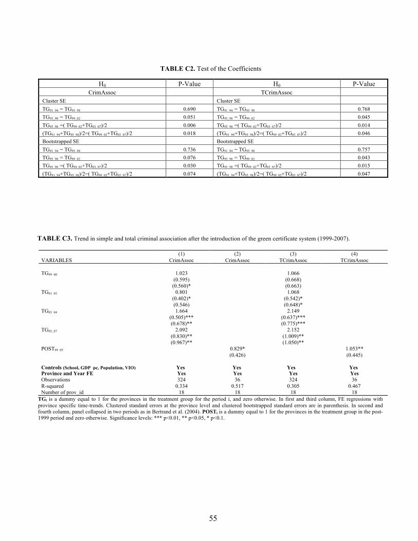
55

TABLE C2. Test of the Coefficients



TABLE C3. Trend in simple and total criminal association after the introduction of the green certificate system (1999-2007).

(1) (2) (3) (4) VARIABLES CrimAssoc CrimAssoc TCrimAssoc TCrimAssoc TG99_00 1.023 1.066 (0.595) (0.668) (0.560)* (0.663) TG01_02 0.801 1.068 (0.402)* (0.542)* (0.546) (0.648)* TG03_04 1.664 2.149 (0.505)*** (0.637)*** (0.678)** (0.775)*** TG05_07 2.092 2.152 (0.830)** (1.009)** (0.967)** (1.050)** POST99_05 0.829* 1.053** (0.426) (0.445) Controls (School, GDP_pc, Population, VIO) Yes Yes Yes Yes Province and Year FE Yes Yes Yes Yes Observations 324 36 324 36 R-squared 0.334 0.517 0.305 0.467 Number of prov_id 18 18 18 18


56

Appendix D. Analysis with a different treatment group (least windy provinces2) and the same control group. TABLE D1. Trend in simple and total criminal association in the whole period (1990-2007).

(1) (2) (3) (4) VARIABLES CrimAssoc CrimAssoc TCrimAssoc TCrimAssoc TG91_94 0.332 1.959 (0.934) (1.163) (0.967) (1.232) TG95_98 0.030 1.463 (1.223) (1.410) (1.251) (1.502) TG99_02 0.288 0.277 2.247 0.482 (1.512) (0.610) (1.517) (0.961) (1.587) (0.499) (1.967) (0.758) TG03_07 0.047 0.141 0.948 -0.969 (1.763) (0.734) (1.855) (1.539) (2.074) (0.762) (2.528) (1.129) Controls (School, GDP_pc, Population, VIO) Yes Yes Yes Yes Province and Year FE Yes Yes Yes Yes Observations 342 342 342 342 R-squared 0.402 0.401 0.359 0.346 Number of prov_id 19 19 19 19

TGi is a dummy equal to 1 for the provinces in the treatment group for the period i, and zero otherwise. FE regressions with province specific time-trends. Clustered standard errors at the province level and clustered bootstrapped standard errors are in parenthesis.Significance levels:***p<0.01,**p<0.05,*p<0.1.

TABLE D2. Test of the Coefficients



2Ragusa, Teramo, Pescara, Caltanissetta, Enna, Reggio di Calabria, Catania, Chieti"

57

TABLE D3. Trend in simple and total criminal association after the introduction of the green certificate system (1999-2007).

(1) (2) (3) (4) VARIABLES CrimAssoc CrimAssoc TCrimAssoc TCrimAssoc TG99_00 0.133 0.460 (0.575) (0.888) (0.548) (0.836) TG01_02 0.700 0.202 (0.785) (1.417) (0.679) (0.969) TG03_04 0.281 -0.975 (0.816) (1.647) (0.679) (1.162) TG05_07 0.431 -1.390 (0.951) (2.040) (0.972) (1.456) POST99_05 0.131 0.143 (0.579) (0.754) Controls (School, GDP_pc, Population, VIO) Yes Yes Yes Yes Province and Year FE Yes Yes Yes Yes Observations 342 38 342 38 R-squared 0.403 0.143 0.347 0.130 Number of prov_id 19 19 19 19


cesifo, a munich-based, globe-spanning economic research ... filevenice summer institute 2014 the...

Documents