ce-str-82-5 effects of gain and delay-time of control

CE-STR-82-5

EFFECTS OF GAIN AND DELAY-TIME OFCONTROL DEVICES TO STRUCTURAL SAFETY

byM. A. Basharkhah

J. T. P. Yao

Any opinions, findings, conclusionsor recommendations expressed in thispublication are those of the author(s)and do not necessarily reflect the viewsof the National Science Foundation.

Supported byThe National Science Foundation

throughGrant No. CME-8018963

January 1982

School of Civil EngineeringPurdue University

West Lafayette, IN 47907

$0272 -101

REPORT DOCUMENTATION 11. REPORT NO.PAGE NSFjCEE-82001

•• Recipient's Accenion No.

PB8~ 19315 2•• Title end Subtitle

Effects of Gain and Delay Time of Control Devices toStructural Safety

50 Report Oet"January 1982

7. Author(s)

M.A. Basharkhah, J.T. Yaoa. Performinl Ora.niz.tion Rept. No.

11. ContractCC) or GrantCG) No.

10. Project/Task/Work Unit No.9. Performina 0ra.niz.tion Name end Address

Purdue UniversityDepartment of Civi'l EngineeringWest Lafayette, IN 47907 CC)

(G)CME8018963

12. Sponsorinl Or.anization Name end Address

M•P. Ga US, CEEDirectorate for Engineering (ENG)National Science FoundationWashinaton DC 20550

13. Type of Report & Period Covered

~---------'-----11•.

15. Supplementary Not".

-----------

Submitted by: Communications Program (OPRM)National Science FoundationWashington, DC 2055~ _

16. Abstract (Limit: 200 words)- _._._-----------1

The effects of several combinations of gain and delay time on the control of suchflexible structures as tall buildings and long bridges are studied. Investigationsof active structural control, active damping of large structures in winds, antiearthquake application of pulse generators, active feedback control, modal synthesis,and modal control are reviewed. To reduce undesirable effects of disturbances, thefeedforward control system, the feedback control system, or a combination of the twomay be used. Ways to minimize the effects of the disturbance force are examined. }An example is provided of a single-degree-of-freedom structural system subjected toan artificially generated earthquake. It is found that the larger the gain and thesmaller the delay time, the more effective the control system will be.

17. Oocument Anelysis e. Descriptors

Structural designEa rthqua kesPulse generators

Buil di ngsSkyscrapersBridges

SafetyStructuresEarthquake resistant structures

b. Identlfiers/Open·Ended Terms

Ground motionStructural control

c. COSATI Field/Group

18. Availability Statement 19. Security Clan (This R"port) 21. No. 01 Pal'"

22. Pricef-------------I-------.-

20. Security Clan (This Pal")NTIS

(Se. ANSI-Z39.18) See 'nstruchons on Reverae OPTIONAL FORM 272 C.-77)(For",,,rly NTlS-3S)Oepartment of Comm"rce

1. Introduction:

The useful life of a fle~ible structure, such as a ship, a tall building,

or a large airplane, depends ,m the possibility aTld probability of fatigue

failures due to the vibration of such structures. Each vibrational mode can

be descrihed with an equation of motion of the form: mx + b~ + kx = U(t),

where U(t) is the input or excitation force. Theoretically, it is possible to

find an input which will drive both the deflection, x(t), and velocity, ~(t),

to zero in finite time for arbitrary initial conditions because such a linear

system is completely controllable.

In the real-world, one is concerned with limited supply of energy which is

required to produce control forces. It is well known that more energy is re

quired for higher gains. Moreover, there always exists a delay time in generat

ing the desired control fC?rce. To study the reliability aspects of the struc

tural control problem [lJ, it is necessary to consider the effects of the gain

and delay time which are inherent in applying control systems to ensure struc

tural safety.

The objective of this study if to find the effects of several combinations

of gain and delay time on structuraL control. To solve the problem, one is able

to use the following two approaches: the classical control theory in the fre

quency domain, and the modern control theory in the time domain.

2. Literature Review:

During these past several decades, aetive control has been extensively

applied in aerospace and mechanical engineering praetices. However, applica

tions to civil engineering structur 's began only in recent years. One reason is

that civil engineering structures t'~nd to be more complex as well as bulkier and

thus more difficult to control. While active contr)l is not advocated for every

structure, there are certain structures for which the use of active control can

result in a more efficient and reliable design.

To control the behavior of a given structure, one can use either passive

and/or active control systems. The main idea of using a control system is that

flexible structures such as extreme]y tall buildings or long bridges

can be designed to resist essentialJy th,' operatlonal gravity loads and the

active control system can take care of any sile-sway motions resulting from

lateral loads. Recently, the relevant 1itera l:ure ;Illd the interrelation-

ship among structural identification, control, and reliability in wind engineer

ing were discussed [2]. In the following, additional literature on this subject

matter is reviewed briefly.

A general approach to active structural control was discussed by M.

Abdel Rohman and H. H. E. Leipholz [3]. They proposed a unified approach to

be used in the active control of structures to satisfy simultaneously the re

quirements for safety, serviceability, and human comfort considerations. The

feasibility of using such a cont 1"01 was also considered. In another paper,

Rohman and Leipholz [4] studied the vibration of a single-span bridge. The

control mechanism has been used to control the vibration of the bridge. They

also showed some of the benefits from using a closed-loop control in controlling

flexible civil engineering structures.

Active damping of large structures in winds was studied by Richard A. Lund

[5]. Mass dampers have been installed in large buildings to reduce bUilding

motion during high winds. These systems are presently designed to operate as

passive tuned mass dampers. An investigation of the benefits of active con

trol in such systems was presented by Lund.

Anti-earthquake application of pulse generators was studied by Sami F.

Masri and George A. Bekey [6]. They used servo-controlled gas pulse genera

tors to mitigate the earthquake induced motions of tall buildings.

The active control of structures by modal synthesis was presented by

L. Meirovitch and H. OZ [7]. Their control scheme consists of independent

2

modal control providing active damping for the controlled modes of the struc-

ture.

The concept of active feedback cont~ol is studied by John Roorda [8].

The first experiment demonstrates in a f;imple way the essential ingredients of

an active feedback control system. It involves the control of the midspan

deflection of a king-post truss by selectively lengthening or shortening the

under-slung cable in a controlled way. In addition, a vertical cantilever is

controlled with a pair of vertical steel tend('Us fixed to a cross arm attached

at the column and to a y()ke which pivots about the column center line near

the base.

Soong and Chang [9] studied an optimal control configuration using the

theory of modal controL For tall buildings, the application of modern con-

trol theory introduces a number of difficult problems. An important problem

is that of obtaining optimal control configuration or the determination of

appropriate locations of controllers. This topic has been studied by Soong

and Chang [9].

Recently, optimal open-Ioop:ontn l of structures under earthquake excita-

tion was studied by J. N. Yang an! M. J. Lin [10]. They used an active tendon

control system and an active mass damper system.

3. Formulation of the Problem

A lumped-mass one-story building \\lith active control devices is shown in

Figure (1). The particular control devices as considered herein consist of a

"jet-engine-like impulse force gEneratn" attached to the top of the building.

The equation of motion for'such a structure can be written in the following form:

.mx + bx + kx = N + u (1)

where N = N(t) is the external excitat Lon SUCll as earthquakes. For example,

N = -mx , where x denotes the ground Lcceleration. In Equation 1, the termg g

3

.u - u(x,x;t) denotes the control force generated with a control device which

is located at the top of the system. The Laplace transfer function of the

plant (structure) can be written as follows:

where:

G (8)P

12

ms +bs+k(2)

m Mass of the systemb Damping of the systemk Stiffness of the spring

Without loss of generality, the e}ternal force can be disregarded for

the subsequent discussions because the external force can be assumed as a

part of u in Equation (1) becomEs:

mx + b~ + kx u (3)

For a single-degree-of-freedom system, Equation (3) can be written in

the following form:

.X /tJ{+ Bu

y ex

where:

;] [;]A~ [0 B e = [1 0]-k

m

Now, the matrix P can be defined in the following form:

(4)

P [B lAB] (5)

Because the rank of the P matrix is equ~l to two, therefore, this system

is controllable (see Appendix A). The systerr is also observable because the

rank of Q matrix is also equal to two. Where Q matrix is defined as:

4

The block diagram of the system without any control device is shown in

Fig. 2. A generalized closed loop system schematics is shown in Fig. 3.

Tn civi.l englneering structllres, tilt' dJ.sl urbnnce force 18 the major 1n-

put force of the system. To reduce the undersirable effects of disturbances,

one can use either the feedl'orward cont rol system or feedback control system.

It is also possible to use both systems at the same time.

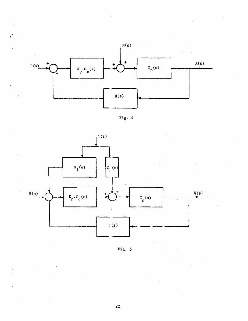
For example, consider the system as shown in Fig. 4 where Kp is an ad

justable gain andG (s) and H(s) are fixe,! components. The closed-loop transc

fer function for the disturbance is:

~(s)

N(s)(7)

To minimize the effect of the dist!lrbance force, the adjustable gain ~

should be chosen as large as poss ble. One cen also reduce the undersirable dis-

turbance force by using a feedfor\lard control. Fig. 5 shows a system with

feedforward control. A disturban~e feedforward is an open-loop and it depends

on the constancy of the parameters. In Fig. 5 both open-loop and closed-loop

control systems are used simultaneously. In this system, errors from all causes

can be reduced without requiring a large loop gain. A feedforward system can

be used if and only if one can m, 'asure the dis turbance forces.

Consider the system as showl in Fig. 5. It has been assumed that both

plant transfer function, Gp(s), and disturban"e transfer function, G2(s), are

known. One can easily find a suitable controller transfer function, GC(s),

then, the disturbance feedforward trans fer fWlction, G1

(s) can be found as

follows:

(8)

Consider the system shown in Fig. if. The transfer function of the

5

system can be obtained as

~(s)

N(s)

Gp(s)

1+K G (-s)<'""":G=-p"'(s"""")=R (s )p c

(9)

The effect of the controller is s('en by the presence of ~ in the denom

inator of the transfer function. From this equatLon, the response ~(s) to

the disturbance force, N(s), can he foulld. On the other hand, in considering

the response to the reference inp Lt R(s), we may assume that the disturbance

is zero. Then the response XR(s) to th,~ reference input R(s) can be obtained

from

(10)

The response to the simultaneous application of the reference input and

disturbance can be obtained by adding the two individual responses. In other

words, the total response Xes) due to the simultaneous application of the

reference input R(s) and disturbance N(s) is given by

Xes) (11)

The reference input R(s) can be assumed to be zero because the set point

of the controller is fixed. Consider now the case where IK-G (s)R(s) 1»1 and-1' c ~(s)

IKGc(S)Gp(s)R(s) 1»1. In this case, the closed-loop transfer function N(s)

becomes almost zero, or as small as possible. This is an advantage of using

the closed loop system. If the referenc(~ input R(s) not. ~(s)

then the closed-loop transfer fmlct10n R(s) approaches

to be equal to zero,

1R(s) as the gain

of KG (s)Gp(s)R(s) increases. Thjs means that the closed-loop transfer function~(s)cR(s) becomes independent of ~C:c(s) ;md Gp(s) an,! becomes inverseley propor-

tional to R(s) so that the varia ions of Gp(s) and KpGc(S) do not affect theXR's)

closed-loop transfer function R(s:r-. This is another advantage of the closed-

loop system. It can easily be seen that any close<I-loop system with unity

6

feedback tends to equalize the input and output.

A lumped mass n-story building with act_ve clntrol devices is shown in

Fig. (6). The particular control devices cOllside oed herein consist of jet-

engine attached to each 1'100'. The equation:; of lotion can be written in the

following form:

my + cy + ky N + bu (12)

in which y is the relative displacement vector, N is the external excitation

vector that it is called disturbance force, l' is the vector of control force.

Each element of u represents either the pushing or pulling force generated by

a control device located at each floor. b is a nXI' matrix whose elements de-

pend on the arrangement of the controller. TIl, C, and k are the mass matrix,

the damping matrix, and the stiffness matrix respectively and they are nxn

matrices.

By using state space concept, Equation ]2 can be converted into a set

of 2n first order differential equation. Note also that without loss of

generali ty, the "external forces or disturbanr = forces can be disregarded and

hence Equation 12 becomes:

.X = Ax + Bu (13)

where: y cx

x= H-} A ~ [-Q-- _!_-J I~ = [-~~]-1 -1-m k -m c

Because the main objective of this investigation is earthquake; one can

neglect the damping of the systen only during the time of the earthquake.

By using the similarity transformation, Equation 12 can be written in

the following form:

.X = AX + Bu

y = cx 7

(14)

where

A B-1

T B and c = Tc

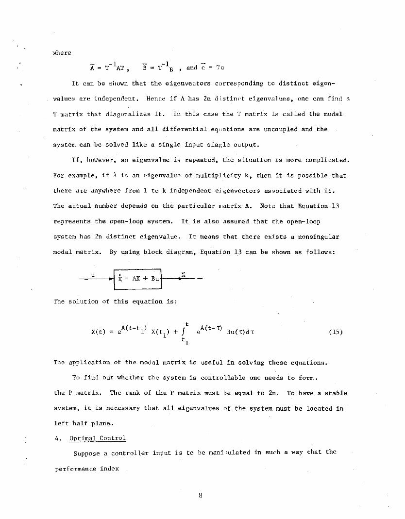
It can be shown that the eigenvectors corresponding to distinct eigen-

values are independent. Hence if A has 2n d istinf't eigenvalues, one can find a

1 matrix that diagonalizes it. In this case the T matrix is called the modal

matrix of the system and all differential eqllations are uncoupled and the

system can be solved like a single input single output.

If, however, an eigenvalue is repeated, the situation is more complicated.

For example, if A is an ('igenvalue of multipJ iefty k, then it is possible that

there are anywhere from I to k independent ejgenvectors associated with it.

The actual number depends on the partjcular matrix A. Note that Equation 13

represents the open-loop system. It is also assumed that the open-loop

system has 2n distinct eigenvalue. It means that there exists a nonsingular

modal matrix. By using block diagram, Equatjon 13 can be shown as follows:

The solution of this equation is:

A(t-1)e Bu (T) d T (15)

The application of the modal matrix is useful in solving these equations.

To find out whether the system is controllable one needs to form.

the P matrix. The rank of the P matrix must be equal to 2n. To have a stable

system, it is necessary that all eigenvalues of the system must be located in

left half plane.

4. Optimal Control

Suppose a controller input is to be maniJulated in such away that the

performance index

8

.J f «Y,QY> + <u,Ru>ldt

o(16)

is minimised for a plant having !;tate-:,pace 1'(lllations

x= AX + Bu

y = ex (17)

where (A,e) is an observable pair. Th, corr(~sponding optimal control action

is given by

u (18)

where P is the unique positive dEfinite soluiion of the steady-state matrix

Riccati equation.

-1-PA-AT1' + PBR BTp = eTQC

This is the negative feedback conventioll form of tile Riccati equation.

5. Numerical Example:

(19)

Consider the control system shown in Fig. 1.

is:

.X = AX + Bu

The equation for the plant

(20)

where:

x = {::}

(21)

9

(22)

The solution of the Riceati equation is:

t1681 .0578)

.057'0 .008

and the optimal control force is:

(23)

u = -[ .1926 .0267]X (24)

6. Discussion·and Conclusions

Consider a single-degree-of-freedom structural system subjected to an

artificially generated earthquake. The properties of this earthquake are

given as follows:

(1) The duration of the record is 15 seconds;

(2) The uniform time interval is .05 sec.;

(3) The exponential decay constant is .62;

(4) The duration of the parabolic buildup time is .5 sec.;

(5) The time at start of exponential dec:lY is 7.5 sec.;

(6) The lowest input spectrum frequency is .1 Hz;

(7) The highest input spectrum frequency is 10 Hz.

( 8) The maximum acceleration is log;

(9) The Maximum velocity is 24 in/sec.;

(10) The Maximum displacement is 5 in.

Moreover, the properties of the system are given as follows:

.3 Kip secm = -2

in

.5 Kip secc = in

K = 2.5 Kip/in

Considering the information as listed in Table (1), it is observed that

by increasing the gain K , one can control the displacement of the system.p

It is also clear that by reducing the displacement the control force will in-

10

crease. The same discussion is valid for the feecback gain. It means that

by increasing the feedback gain, H, the displacem£nt of the response will de-

crease. If the feedback gain is set to be .20, a nearly optimal solution can

be obtained. However, the redUt~tion of the d lsplacement is not very much.

Of course, by changing the "Q" we may filld another gain that it may give a

desire displacement. Result as summarized in Table (1) are shown in Fig. (8)

through 15.

Fig. (8) shows the behavior of the systemwit:hout active control force.

The top plot is the external force, which is the product of mass and the

ground acceleration. The active control force and displacement of the response

have been plotted. It can be se£n that the control force is equal to zero and

the maximum displacement is equa] to -3.32 inches. By using the active control

force, the response displacement becomes sm~ller than the displacement of the

system without active control syf:tem. Note that by increasing either the gain

K or the feedback gain, H, or both, the response of the system becomes smaller.p

In Table (1) an unity feedback control system is used, and only the behavior

of the system with respect to changing M the gain K is shown. Fig. (9) showsp

the active control force and displacement of the response when K is equal top

.20. The maximum displacement in tllis cuse is -3.30 in. It is obvious that

the required active control force is small and also the displacement does not

change very much.

Fig. (10) shows the same system K is equal to one and the maximum disp

placement is -3.06 inches. The active control force has been increased in

this case. The maximum displacement in Fig. (11) is equal to 3.22 inches and

the value of the active control force has been increased.

By choosing K to be equal to 5.0, the maximum displacement is found top

be +3.14 inches. When K is equal to 10, the maximum displacement is +2.9p

inches. Due to higher gains such as K = 25 or K = 100, the maximum displace-p p

ments became smaller. In these last two cases the maximum displacements are

11

respectively ~2.32 inches and +1.27 inches. These refults are shown in Fig. (12)

thru (15). Note that the transfer function of the cal troller has been assumed

as a constant gain, K ,. If we assume that the transjer function of the jetp

engine to be

system mayor

1T s+l

amay not

we may have the same results but it is obvious that the

be stable. By changing T , we Ilay have an unstablea

system. Table (2) shows the result of the same syste, when the transfer

T s+l •a

The only

1

The value of H, K have been chosen as J. and 1. respEctively.p

variable of the system is T and the rpst of the paraneters are constant.a

function of the controller has been assumed as followf: G (s) =c

Assuming T equal to zero, we will have a maximum displacement equal to .179".a

By increasing the value T , we will have a higher valt e for the displacement.a

For example, Fig. (18) shows the displacement of the lesponse when T isa

equal to .OOL In this case, the maximum displacement is equal to .180" and

it is greater than the maximum displacement with T equal to zero. Fig. (19)a

shows the plot of the active control force for this CEse. Note also that the

system is stable because all eigenvalues have a negati ve real part. Fig. (20)

shows the behavior of the same system when T has been chased as .005. Thea

displacement of the system is higher than both previous cases with maximum value

of .181". The active control force for this case has been shown in Fig. (21).

Fig. (22) thru (30) show the behavior of the system by increasing the value of

T •a

The displacement of the system has become larger. Due to some value of T ,a

we may have an unstable system. For ('xample, hy choosing T equal to .5 we havl~, . a

an unstable system. The displacement of the system at time t = 20 sec. is

equal to .966". Fig. (28) shows the response of this sytem. In this case, we

have two eigenvalue with positive real part. By increasing the value of T toa

one, the system becomes stable and all eigenvailles have a negative real part.

Note also that the maximum displacement of the system without any active con-

trol force due to the same external force, stn2t, is equal to .60". By in-

creasing the value of T , the displacement becomes larger. Notice that ina

12

most cases the value of the displacement is smaller than the value of displace-

ment without any active control force unless the system becomes unstable. For

example, by chossing T equal to 1. although we have a stab Ie system, but thea

displacement of the system with .lctive control system Ls gl ~ater than the dis-

placement without any activ(~ con:'rol system. It mean~; that by using active

control system the performance of the system is much worse ~han performance

of the system without active control force, and note ;i1so tilat the stability

of the system is important.

In this report, the effects of gain and dday time are studied. General-

1y, the larger the gain and the ~;ma11f'r the de Lay time, the more effective will

be the control system. In the real world, there exist practical limitations

as to the upper bound of the gain and 1he lower bound of the delay time. The

structural reliability as a functLon oj these factors is being studied in

more detail and will be presented in the next technical report.

Acknow1ed&ment

This investigation is supported in part b:' the National Science Foundation

through Grant Number CME-8018963. Authors wish to thank Drs. M. P. Gaus and

J. E. Goldberg for their advice and encouragement. Mrs. Vicki Gascho capably

typed this manuscript.

13

APPENDIX: Controllability an,! Observability of Linear Systems

The linear system as represented by the following equation of motion,

.X = AX + Bu

with the following solution:

(A-I)

(A-2)

is said to be controllable at time to if there exists u(a), to ~a~tl' which

satisfies A-2 for arbitrarily specified vectors, X(tl), X(t

O)'

One can show that u(a) is a control which satisfies A-2 for arbitrary

X(tl

) and X(tO). u(a) is given by following equations:

u(a)

and

(A-3)

Theorem:

(A-4)

.The linear system X = A,,{ + Bu is controllable at to if and only if there

exists a finite tl>tO such that

(A-5)

X(tl,tO

) is called the controllability matrh, and one can ~how that X(t,tO)

satisfies the following equation:

* *= X(t,tO)A (t) + A(t)X(t,tO) +B(t)B (t) (A-6)

For a time-invariant system, both matrices, A, B, are constants. Using

Cayley-Hamilton theorem we have:

14

Theorem:

A linear time invariant system is contr01lable only if rank P = n

where P is a matrix as follows:

[P] (A-7)

There is another theorem for controllability I)f a linear-time-invariant

system. If A, B are constants, then the linear system is controllable if

and only if X(oo,O»O, or

00 *X(oo,O) = J eAtBB*e' tdt>O

o

and if A is stable X(oo,O) satisfie.s

* *X(oo,O)A + AX(oo,O) + BB = °Therefore there are two controllability criteria as follows:

Controllability Criterion 1

(A-B)

(A-9)

The constant coefficient syste~. for which A has distinct eigenvalues,

is completely controllable if and only if there are no zero rows of B = T-IB,n

where T is the modal matrix.

Controllability Criterion 2

A constant coefficient linear system with the representation {A,B,c,n} is

completely controllable if and only if the matrix of

(A-IO)

Consider the following single-degree-of-freedom mechanical system:

:H~ + BX + KX = u

15

where:

-Ka =""11

-Bb =M

1c =-If

It is obvious that rank p = 2. Therefore, the system is controllable.

In this example the disturbance force has been ignJred.

Observability of Linear Systems:.

The linear system X = AX, Y = eX with solution

yea) = c(a)~(a,t)X(t), a>t (A-ll)

is observable at time t if there exists some I:l>t such that X(t) can uniquely

be determined by measuring yea).

The linear system is obs~rvable at time, t, if and only if there exists

a finite t1

>t such that K(t1,t»o where K(t

1,t) is given by:

t 1 * *J ~ (a,t)c (a)c(a)~(a,t)dat

(A-12)

X(t)-1

= K(tl

, t) Itl * *~ (a,t)c (a)y(o)da

t(A-13)

K(t1,t) .is called the observability matdx and it must satisfy the follow

ing differential equation.

K(t,t) a (A-14)

Observability for time-invariant systems depend only on the constant

matrices A and c. No reference need be made to a particular interval [to,t l ].

16

Observabi1ity Criterion 1

The constant coefficient system, for whjch A has distinct eigenvalues,

is completely observable if and only if there are 10 zero columns of c = cT.n

where T is the modal matrix.

Observabi1ity Criterion 2

A constant coefficient linear system is comp1(~te1y observable if and only

if the nxmn matrix, Q, has rank n:

**I * *I n-1"/<Q~[c A c -----~A c] (A-1S)

If both matrices A and c are constant then the linear time-invariant system

is observable if and only if

K(OO,O)~*

Joo A t * Ate .c .c.e dt>Oo

(A-16)

If A is stable then K(oo,O) satisfies

* *K(oo,O)A + A K(oo,O) + c c = 0 (A-17)

The controllability as well as observabi1ity of a linear time-invariant

system is invariant under andy similarity transformation.

As an example, consider the single degree freedom system. The equation

of motion is given by:

17

In this case the output of the system is displacement.

Qll[cT,ATcT,----

Q -(: :)rank Q = 2

It is obvious that the rank Q is two, th3refore the system is observable.

18

References:

[1] Yao, J. T. P., "Identification and Control of Structural Damage", SolidMechanics Archives, Vol. 5, Issue 3, Sijthoff & Noordhoff InternationalPublishers, Netherlands, August 1980, pp. 325-345.

[2] Yao, J. T. P., "Structural Identification, Control, and Reliability inWind Engineering Research", Technical Report No. CE-STR-8l-9, School ofCivil Engineering, Purdue University, W. Lafayette, IN, April 1981.

[3] Abde1-Rohman, M., and Leipholz, H. H.E., "A General Approach to ActiveStructural Control", Structural Contro1, edited by H. H. E. Leipholz,North-Holland/SMPublications, 1980, pp 1-28.

[4] Abdel-Rohman, M., and Leiphc'lz, H. H. E., "Automatic Active Control ofStructures", Structural Contro1, edited by H. H. E. Leipholz, NorthHolland SM Publications, 19~;O, pp 29-56.

[5] Lund, R. A., "Active Dampin~, of Large Structures in Winds", StructuralControl, edited by H. H. E. Leipholz, North Holland/SM Publications,1980, pp 459-470.

[6] Masri, Sami F., Bekey, George A., Safford, Frederick B., Dehghanyar,Tejav J., "Anti-Earthquake Application of Pulse Generators", DynamicResponse of Structures, edited by G. C. Hart, American Society of CivilEngineers, Jan. 1981, pp 87-101.

[7] Meirovitch, L., and tlz, H., "Active Control of Structures by ModalSynthesis", Structural Control, edited by H. H. E. Leipholz, North-Holland/SM Publication, 1980, pp. 505-521.

[8] Roorda, J., "Experiments in Feedback Control of Structures", StructuralControl, edited by H. H. E. Leipholz, North Holland/SM Publication, 1980,pp. 613-627.

[9] Soong, T. T., and Chang, M. K. J., "Optimal Control Configuration inTheory of Modal Control", Structural Control, edited by H. H. E. Leipholz,North-Holland/SM Publication, 1980, pp. 723-738.

[10] Yang, J. N., and Lin, M. J., "Optimal Open J"oop Control of StructuresUnder Earthquake Excitation", Structural Safety and Reliability, editedby T. Moan and M. Shinozuka, Elsevier Company, 1981, pp. 751-760.

[11] Modern Control Engineering, Katsuhiko Ogato, Prentice-Hall, Inc., Englewood Cliffs, NJ.

[12] Modern Control Theory, William L. Brogan, Quantum Publishers, Inc.

19

TABLE (1)

Case Fig. T H KMax. Max. Max.

a p Displacement Velocity Ace.

1 8 .00 0.00 0.00 -3.32 23.14 -372.24

2 9 1. .20 -3.3 23.40 -373.84

3 10 .00 1. 1.0 -3.06 -24.68 -377.67

4 11 .00 1. 2.0 3.22 -25.66 387.55

5 12 .00 1. 5.0 3.14 -24.13 429.17

6 13 .00 1. 10. 2.9 -24.78 451. 57

7 14 .00 1. 25. -2.32 -28.83 463.93

8 15 .00 1. 100. 1. 27 22.74 525.89

TABLE (2)

Case Fig. N T H KMax.

a p Displacement-

9 16 Sin2t O. 5. 1• .17987

10 18 Sin2t •001 5. 1. .18017

11 20 Sin2t .005 5. l. .18137

12 22 Sin2t .01 5. l. .18291

13 24 Sin2t .05 5. 1. .19654

14 26 Sin2t .1 5. l. .2143

15 28 Sin2t •5 5 . 1. .86574

16 30 Sin2t 1. 5. 1. .6056

20

;;;I,},.;,;,

u(t)

I~...

Fig. 1

N 1+.____ 1O------G (s) = -~--p ms 2+cs+k

X(t)

Fig. 2

RN: Disturbance

ut+ Outp

) Controller Actuatpr r--O--- Plant,

MeasuringElement

+

Fig. 3

21

N(s)

R(S)~....+..cK .G (8)

P C

,------{

+ + XeS)G (s)

p

R(s) ....

Hs)

Fig. 4

G1

(8) G., (s

K .G (s)P c

+ +G

p(s) !

~ .-JXes)

'-------1 ':]-------'

Fig. 5

22

Un

_l1---------4.-....,..

U

J----------1~

Fig. 6

ooo

ooo.C\J

I

ooo>-.::r

1

ooo(D

1

--------- ~.~_.. "',--- ._----_.__._-

ooo-+_~

~10 .00I

-5.00 .00 5.00I

10.00

Fig. 7. Nyguist Plot of the Open-Loop System.

23

\.

External Force. 100.0

0.0

-100.0

-200.0-f-----.---:.---.-----,-----.-----r---..--...,.--..-----,1.000~.OO 2.00 4.00 6.00 8.00 10.00 12.00 14.00 16.00

Tlr~E

.600 Coot rol Force

(f)0.......~

O.OOO-i------------------------------

-.500 -t------r------r------r---~·--rl-----rl------rl----jr-----llO.OO 8.00 lO.OO 12.00 14.00 16.00

TIME

. Displacement of the Response

xmax = -3.326.00

•:cuz.....0.00 ~\

-5.00 -+------.-------.-------./-----,-1----,-,-----.,----'.-------.1D.Oo- 2.00 4.00 6.00 3.00 10.00 12.00 14.00 16.0J

TIME

Fig. 8

External Force, Control Force, and Displacement Responsefor Case 1 in Table 1.

24

External Fa rce100.0

0.0

-100.0

-200.0 -4------.------..-----.----r-1.000

J10.00

I12.00

I14.0b

IlE.OO

Control Force

-.500 -+------.------r-----.----or--o---.,-j------.'----rj---~I10.00 10.00 12.00 14.00 16.00

.500

0.000

(f.)(l.......~

:I:UZ.....

5.00

0.00

Displacement of the Response

xmax = -3.30

I16.00

I14.00

i12.00

j10.008.00

TIME6.004.002.00

-5.00 -+-----,--'----r----,----,--0.00

Fig. 9

External Force, Control Force, and Displacement Responseo for Case 2 in Table 1.

25

-200,0 -t-----r-----,-.---,------,Ir----rl---~I-----,1----"~·---,I10.00 6.00 8.00 10,00 12.00 14.00 16.00

TIME

5.00 Control Force

(f)lL.....~

0.00

-5.00-+----,,-----.-----.-----.-----.-----.-----.-----.10.00

.:cuz.....

6.00

0.00

'Displacement of the Response

xmax = -.3.06

16.0~ILI,OO12.00to.oo8.00TIME

6.004.002.00-5.00-+-----.-----.--,---,----r----.----.-----,-----,

0.00

Fig. 10

, .

External Force, Control Force,and Displacement Responsefor Case 3 in Table 1.

26

External Force100.0

0.0

-100.0

~,

~ ~ i' I 1 J V .

-200.0 -1----~---__r----___,I-----rj-------,.'----r-I----,-,~---'I20.00 6.00 8.00 10.00 12.00 14.00 16.00 .

TIME

10.00

0.00

Control Force

-10 .00 +----y-----y----_,_---_,_---:---r----,-----,-----,10.00

.J:UZ~

5.00

0.00


xmax - 3.22

-5 .00 -+-----r----.,-~---,-------.I----i'----r-, -----.1------.,0.00 2.00 4.00 6.00 8.00 10.00 12.00 14.00 16.CD

TIME

Fig. 11

External Force, Control Force, and Displacement Responsefor Case 4 in Table L

27

(f)0........~

100.0

0.0

External Force

-100.0

-200.0 -f-----r-----r'-----.I----'I-40.00 4.00 6.00 8.00

TIME

. I10.00

I12.00

,14.00

,16.00

(f)0.........~

20.00

0.00

C0'1tro1 Force

,~v~-,-

-20.00-+-----r-------rI-----.'----'I-----r'-----.,-----r,----,10.00 Lf.OO 6.00 8.00 10.00 12.00 lIi.OO 1£'.00

TIME

.J:UZ.....

6.00

0.00

'Displacement of the Response

xmax = 3.14

-5.00 +.c.----,-----,-----...----.-- ----,'r----r,------r:-----"0.00 2.00 4.00 6.00 8.00 10.00 12.00 Il ;.OO 16.00

TIME

Fig. 12


28

UJ0.........~

100.0

0.0

External Force

-100.0

-200.0 +----.-----.-----,-----.-1-----,r-----r-I-----,-j-----,1100.0 8.GO 10.')0 12.00 14.00 16.00

TIME

60.0Control Force

UJD.-......~

0.0

-50.0 +----.-----'Ic----,'r----.I---.-1-----..1----.,.1----,10.00 4.00 6.00 8.00 10.00 12.00 14.00 In.CO

TIt~E

.:r:uz.....

6.00

0.00


xmax = 2.9

-5.00 4-----.-------.-------.-----,---.----,-----,-----,-------,0.00 2.00 4.00 6.00 8.00 10.00 12.00 14.00 Ie r:n

TIME

Fig. 13


29

100.0

0.0

(f)Q.........~

-100.0

External Force

JL---r-----r---,----.:r=----:!-;:----;;r;--~G;_--~I~200.0 16.00200.0

Control Force100.0

(f)Q.........~

0.0

I I I I-100.0 I I12.00 14.00 If.OO4.00 6.00 8.00 10.005.00 .00 2'.00

TIMEDisplacement of the Response

xmax = -2.320.00

J:UZ......

-5.00

-IO.J I I I II I. I I10.00 12.00 14.00 16.004.00 6.00 8.000.00 2.00

TIME

Fig. 14


30

100.0

0.0

-100.0

External Force

-200.0-+-----r-----r------,1----.1r-------r----.-,-----r-I----"400.0 6.00 8.00 °W.DO 12.00 14.00 16.00

TIME

·200.0

0.0

Control Force

-200.0 -+------.'.------.1...------".------.'.-·---(.------.-,-----,1-----'\4.000 .00 2.00 4.00 6.00 8.00 10.00 12.00 14.00 \6.00

TIME

.:cuz.....

2.000

0.000


xmax = 1.27

-2.000 -+-----.,..-----.,..------.-----.---..---'I------.,Ir----.'...------"0.00 2.00 4.00 6.00 8.00 to.OO 12.00 14.00 16.00

TIME

Fig. 15


31

2.000 EXTERNRL FClRCE

External Force, Velocity, and Displacement Responsefor Case 9 in Table 2.

32

oIf)

o

o(Y")

o

CONTROL FORCE .US. TIME

o--J

o

=:JSo

I

o(Y)

oI

oIf)

o'0.00

I4.00

I8.0, !

1

Fig. 17

I12.0

I

J 6. 0

Case 9 in Table 2.

33

2.000 EXTERNRL FClRCE

I.OOl

0)

~ .000XC

2.001.00.00-1.000 +-----.-------.-"'--~_.-__,_"-,--'''''...L.._.---.,-----,----"'-'""-r-----,

3m ,m sm 6m 7m 8m 9m wmTIME

1.000 -

.500ulLJ0)

"-ruz..... .000

VELOCITY OF THE RESPONSE

-.500 -------,-- I I i I I i I I I.00 1.00 2.00 3.00 '.00 5.00 6.00 7.00 8.00 9.00 10.00

TIME

.'000 -

.2000 DISPLRCEMENT OF THE RESPONSE

I xmax= .1802uz

.0000

-.2000 I i I I I I I I I.00 1.00 2.00 3.00 '.00 5.00 6.00 7.00 8.00 9.00 W.OO

TIfiE

Fig. 18

External Force ~ Velocity, and Displacement Responsefor Case 10 in-Table 2.

34

oo

owo

oN

o

owo

I

oo

CONTROL FORCE .US. TJME FOR CASE

, 0.00 2.00 4.00T

I6.00

Fi g. 19

I8.00

I10.0

Case 10 in Table 2.

35

2.000 EXTERNRL FCJRCE

1.000

to /0... .000~

'<::

2.00I .00.00-I.OOO+-------.----.--:"---'~__._- ~----.---"'-.«-.------,---__r-~~--___.

3.00 ~.OO 5.00 6.00 7.00 8.00 9.00 10.00TIME

1.000

DISP~RCEMENT OF THE RESPONSE

VELCCITY GF THE RESPONSE

3.002.001.00+---..,--------,----,------.,-------"r--- ------r-----r,--.....--......'--.....I

~~ 5~ 6~ 7~ 9~ 10mTIME

-t---...,----,-- ---;,---,..----r-,- --T',---.-'----;I----rl-----"1.00 2.00 3.00 ~.OO 5.00 6.00 7.00 8.00 9.00 10.00

TIME

U .500

W(f)

"ru~ .000

-.500.00

.~OOO

.2000

ru~

.0000

-.2000.00

Fig. 20


36

CONTROL FORCE .US. TIMEoo-<

oCD

o

o(\J

o

oCD

oI

oo

'0.00 4.00 --r--- _..-/ -----,.., ,8.00 12.0 16.0 20.0T

. Fig. 21

Case 11 in Table 2.

37

2.000 EXTERNRL FORCE

1.000·

tJ)0... .000~

:>::

-1.000 ---,.00 1.00 3.00 q.OO 5.00 6.00 7.00 B.OO 9.00 10.00

TIME

1.000

U .500 VELOCITY DF THE RESPONSEllJtJ).....:r:(.jz~ .000

-.500 --,.00 1.00 2.00 3.00 ~.OO 5.00 6.00 7.00 B.OO 9.00 10.00

TIME

.qOOO


:r: xmax=.1829(.jz~

.0000

-.2000 I I I I I I ( (.00 1.00 2.00 3.00 4.00 5.00 6.00 7.00 B.OO 9.00 10.00

TIME

Fig. 22

Externa1 Force, Velocity, and Displacement Responsefor Case 12 in:·Table 2.

38

oo


o<.0

o

oN

o

.o

I

owo

I

oo

'0.00 4.00 8.00T

J2.0

Fig. 23

I16.0

I20.0

Case 12 in Table 2.

39

2.000 E\TERNRL FORCE

1.000

if) j0... .000.....""

-1.000 . ------,.00 1.00 2.00 3.00 ~.OO 5.00 6.00 7.00 B.OO

TIME

1.000

.50(1- VELOCITY OF THE RESPONSEu

If'w(f)

"-:r:uz~ .000

I ---r-- I I I ( I , ----,.00 1.00 2.00 3.00 ~.OO 5.00 6.00 7.00 B.OO 9.00 10.00

TIME

.~OOO


ti xmax=.1965

/z~

.0000

-.2000 I I I I I I I I I ---,.00 1.00 2.00 3.00 ~.OO 5.00 6.00 7.00 B.OO 9.00 10.00

TIME

Fi g. 24


40

oo CONTROL FORCE .US. TIME

oCD

o

oN

o

oCD

0-1

oo

------"r--__ ------r--,12.0 16.0 20.0

4.0010.00--1-+--__----,- -;,r---__

8.00T

Fig. 25

Case 13 in Table 2.

41

2.000 EXTERNRL F1JRCE

/8.007.006.005.00

TIME4.003.002.00

+----,-----T--"""...L.- -,--------r---,--"-L-.,-__-,--__---,_"":O"'..L-.,--------,9.00 10.00

1.000

(/)(L .000~

XC

-1.000.00

2.000

• 1.000UILl(/)

"-:r:uzH .000-

VELOCITY OF THE RESPONSE

42

ooN


oN

o<:t-

o

:=J~

0,

\;0N

-,I

ooN, 0.00

J

4.00I

8.00T

2.0I --~

16.0 20.0

Fi g. 27

Case 14 in Table 2.

43

2.000 EXTERNRL mRCE

2.001.00

\-\----r--- ._-.,.--"--"'-_. ,---.-'--.-~ ---,..----.,-----"'-""......,-----.

,;.00 ~.OO 5.00 6.00 7.00 B.OO 9.00 10.00TIME

1.000 -

UJ(L .000~

-1.000.00

~.ooo -

• 2.000- VEl DeITY OF THE RESPONSE

u VuJ

~ .~

~:L~~ -"--- 1----,-----.'-----"---.,---,,---,,---.".00 1.00 2.00 :.00 ~.OO 5.00 6.00 8.00 9.00 10.00

TI~lE

2.000

1.000 DI~;pLRCEi'1ENT OF THE RESPONSE

:r:UZH

.000

xmax=.865

~·~~V-1.000 , -,--- I -----,-- I , , I I --,

.00 1.00 2.00 3.00 ~.OO 6.00 6.CILJ 7.00 B.OO 9.00 10.00TUlE

Fig. 28


44

oo-i


ooill

ooN

=:J8N

I

0 V0

illI

oo-i

'0.00r-------I-- ..-- -r- --~.

4.00 8.00 12.0 13.0T

I20.0

Fi g. 29

Case 15 in Table 2.

45

2.000 E> TERNRL FClRCE

1.000

<fJ \lL .000.....:.::

-1.000 .~, \.00 1.00 3.00 ~.OO 5.oa G.OO 7.00 8.00 9.00 10.00

TIME

~.ooo

• 2.000uW<fJ

J:uz..... .000

VELClCITY OF THE RESPClNSE

.00-2.000+----.,----,,---,-,- ------,----,-

I~ 2~ 3~ ~~ 5~

TIME

,,---'-,----"---,,-----,6.00 7.00 8.00 9.00 10.00

i10.00

,9.00

I8.00

i7.00

,6.00

DISPLRUcMENT OF THE RESPClNSE

xmax=.6056

~1.00.00

.000

1.000

2.000

-1.000+----,---- I ----,,-----,---,-

2'[',1 3.00 ~.OO 6.lIOTIMe

:r:uz.....

Fig. 30

External Force,Velocity, and D splacement Responsefor Case 16 in "able 2.

4ti

o CONTROL FORCE .US. TIMEoN

r

I

I1

. I

!, I\1

\\ il I

VCJ('j

-,,

('j--I--

, 0.00--'1 .- - . -.J,--.---

4.00 8.00T

I

2.0J

16.0-----,

20.0

Fi g. 31

Case 16in Table 2.

4/

" -':

l- 81-3

81-4

81-5

81-6

81-7

81-8

81-9

81-10

81-11

81-12

81-13

81-14

81-15

81-16

81-17

81-18

81-19

81-20

81-21

81-22

81-23

81-24

81-25

81-26

81-27

81-28

81-29

81-30

81-31

81-32

81-33

81-34

81-35

81-36

81-37

81-38

82-1

82,..2

82-3

82-4

82-5

82-6

82-7

82-8

'~~

STRUCTURAL ENGINEERING TECHNICAL REPORTS

"NFEAP - General Description, Sample Problems and User's Manual (1980 Version)", by S. S. Hsieh, E. C. Tingand W. F. Chen.

"Evaluation of Seismic Factor of Safety of a Submarine Slope by Limit Analysis", by C. J. Chang, W. F. Chen andJ. 1. P. Vao

"Inexact Inference for Rule-8ased Damage Assessment of Existing Structures", by M. Ishizuka, K. S. Fu, andJ. T. P. Vao. (DS80-235913)

"Theoretical Treatment of Certainty Factor in Production Systems", by M. Ishizuka, K. S. Fu, andJ. T. P. Vao. (PB81-236457)

"Dynamic Stability of Curved Flow-Conveying Pipes", by E. C. Ting and Vi-Chen Liu.

"Cyclic Behavior of Tubular Sections", by S. loma and W. F. Chen

"Structural Identification Control and Reliability in Hind Engineering Research", by J. T. P. Vao.

"Damage Assessment and Reliability of Existing Buildings", by J. T. P. Vao.

"Bibliography on Folded Plates (Theory, Material and Construction)" by C. D. Sutton and M. R. Resheidat

"NFEAP - General Description, Sample Problems and User's Manual (1980 Version) Part II", by S. S. Hshih,E. C. Ting and W. F. Chen.

"Recent Advances on Analysis and Design of Steel Beam-Columns in USA", by W. F. Chen.

"Assessment of Seismic Displacements of a Submarine Slope by Limit Analysis", by C. J. Chang, W. F. Chenand J. T. P. Vao.

"Hystereses Identification of Multi-Story Buildings", by S. Toussi and J. T. P. Vao (PB8l-235921)

"Inelastic Cyclic Analysis of Pin-Ended Tubes", by S. Toma and W. F. Chen.

"Cyclic Analysis of Fix-Ended Steel Beam-Columns", by S. Toma and ~J. F. Chen.

"Response of Truss Bri dge to Travel i ng Vehi c1e", by E. C. Ti ng and J. Geni n.

"Identification of Structural Characteristics Using Test Data and Inspection Results", by J. T. P. Vao

"Lateral Earth Pressures on Rigid Retaining Halls Subjected to Earthquake Forces", by t1. F. Chang and W. F. Chen.

"Constitutive Relations and Failure Theories (Chapter 2)", by W. F. Chen (Chairman), Z. P. Bazant,·D. Buyukozturk,T. V. Chang, D. Darwin, T. C. V. Liu and K. J. Willam.

"A Numerical Approach For Flow-Induced Vibration of Pipe Structures", by E. C. Ting and A. Hosseinipour.

"SeismiC Safety Analysis of Submarine Slopes", by C. J. Chang, ~I. F. Chen and J. 1. P. Vao.

"Inference Procedure with Uncertainty For Problem Reduction Method", by M. Ishizuka, K. S. Fu and J. T. P. Vao.

"Serviceability and Reliability of Antenna Structures in Part I: Theory", S. H. Wang, J. 1. P. Vao and W. F. Chen.

"Fuzzy Statistics and Its Potential Applications in Civil Engineering", by J. T. P. Vao, K. S. Fu, M. Ishizuka.

"A Rule - Inference t·1ethod for Damage Assessment", by M. Ishizuka, K. S. Fu, and J. 1. P. Vao.

"Lateral Load Capacity of Structural Tee X~Bracing", by A. D. M. Lewis and K. Nematollaahi.

"StabHity of Structural Members with Time Dependent Material Properties", by E. C. Ting and W. F. Chen

"Response of Plate Bridges to a Moving Mass", by J. Genin, E. C. Ting & Mehdi Ilkhani-Pour

"Probabilistic Methods for the Evaluation of Seismic Damage Of Existing Structures", by J. T. P. Vao

"Lok-Test - A Non-Destructive Concrete Compres'sive Test", by S. Mofid, W. F. Chen, N. J. Gutzwiller

"Cyclic Inelastic Behavior of Steel Tubular Beam-.Columns", by D. J. Han and W. F. Chen"Plasticity in Reinforced Concrete", by ~1. F. Chen

"Fati gue Rel iabil ity of Structures Under Combi ned loadi ng", by Wang Di an-Fu and J. 1. P. Vao

"SPERIL I - Computer Based Structural Damage Assessment System"., by M. Ishi zuka, K. S. Fu and J. 1. P. Vao

"Elastic-Plasti c-Fracture Analysi s of Concrete Structures", by H. Suzuki and W. F. Chen

"Strength ofH-Columns with Small End Restraints", by E. M. Lui and W. F. Chen

"Cap Models for Clay Strata to Footing loads," by E. Mizuno and W. F. Chen

"Plasticity ~lodelsfor Seismic Analyses of Slopes," by E. Mizuno and W. F. Chen.

"Plastic Analysis of Slope with Different Flow Rules," by E. Mizuno and W. F. Chen.

"Large-Deformation Finite-Element Implementation of Soil Plasticity Models," by E. Mizuno and W. F. Chen

"Effects of Adjustable Gain and Delay Time of Control Systems to Structural Safety," by M.A. Basharkhahand J. T. P. Vao.

"Analysis of Steel Beam-to-Column Flange Connections," by K. V. Patel and W. F. Chen.

"Nonlinear Analysis of Steel Beam-to-Column Web Connections," by K. V. Patel and W. F. Chen.

"Accessories to NONSAP Program," by K. V. Patel and W. F. Chen.

ce-str-82-5 effects of gain and delay-time of control

Documents