causal diagrams and bias for posting - university of …shahar/causal diagrams and bias for...

Causal diagrams and three pairs of biases

1

Causal Diagrams and Three Pairs of Biases

Eyal Shahar and Doron J. Shahar

1. Introduction

An association between variables is an idea whose meaning is usually grasped intuitively. In most minds, the statement “Variables D and E are associated” does not call for an explanation. Far less clear is the meaning of causation on which volumes have been written by both philosophers and scientists. Courses in epidemiology teach students to recite the mantra ‘association is not causation’, which is true of course—the words are not synonyms— but the two ideas are connected, and one may be developed from the other.

Considering association to be a basic idea, we define causation as a special type of association between two time‐point variables: an association that is directed forward in time. It is often depicted by a single‐headed arrow pointing toward a later time. If E is antecedent to D, then E D denotes “Variable E is a cause of variable D”. If F follows E and is antecedent to D, then E F D denotes “Variable E is a cause of variable D via an intermediary variable F”. All branches of science, from particle physics to cancer epidemiology, share a single theme: the study of causation.

The effect of E on D is defined as the strength of the causation between E and D. We can estimate the magnitude of that effect (which may be null or negligible) by studying the association between the two variables. In some cases, estimating the marginal (‘crude’) association between E and D would suffice; no further action is needed. Often, however, other variables should be taken into account. A causal diagram—a set of variables and arrows (Pearl, 1995)—clearly explains what should be done to estimate a particular effect. Moreover, causal diagrams help to clarify a long‐standing confusion about the taxonomy of biases (Sackett, 1979 ; Grimes & Schulz, 2002). In fact, almost any claim of bias can be depicted in a diagram.

If causal diagrams are such a powerful tool, can’t science be turned into a computerized algorithm of discovery? Unfortunately, no. To estimate the effect E D, we have to display background causal theories in the form of other arrows; those arrows are often the subject of heated exchanges about sources of bias. No computer program can replace the human debate, and no verdict should be issued either. It is always possible that some critical variables were displayed incorrectly, or not displayed at all. Moreover, scientists often struggle with an inevitable trade‐off between bias, variance, and effort. For example, reducing bias costs extra variance and reducing variance costs extra bias. No algorithm can strike a balance between the two. It is a human decision.

2. Effect modification

The effect E D might depend on the value of another cause of D, say Q (Q D). For instance, the harmful effect of heparin injection (E) on bleeding (D) could depend on aspirin use (Q): heparin might have a stronger effect on bleeding in the presence of aspirin in the blood than in its absence.


2

This phenomenon is called effect modification; Q is called an effect modifier (Shahar & Shahar, 2010a). Effect modification of E D by Q requires Q to have at least one value (say, Q=1), such that the effect E D when Q=1 differs from that effect when Q=q≠1. If Q takes more than two values, the effect E D might be unique to each value of Q. In the general case of multiple modifiers, every combination of their values might dictate a unique effect. For instance, the effect of heparin on bleeding could vary according to the combined values of aspirin use (yes, no), sex (male, female), genotype (A, B, C), and weight (continuous). The simple idea of effect modification opens the door to endless variations.

So far we have considered E D to be the effect of interest and Q (Q D) to be the modifier. But the causal situation of E and Q is symmetrical: E D Q. The variable Q does not have some special property of a modifier which E is lacking. Indeed, we may consider Q D to be the effect of interest and E to be the modifier. Effect modification is therefore a reciprocal phenomenon (Shahar & Shahar, 2010a): given two causes, E and Q, of some outcome, E modifies Q’s effect if and only if Q modifies E’s effect.

To depict a theory of effect modification of E D by Q, we will place the lower case q above the arrow E D. That intuitive notation indicates that the effect behind the arrow depends on the value of Q. Given reciprocity, we should also place the lower case e above the arrow Q D. An arrow with no letter denotes a theory of no effect modification; E has the same effect on D for every value of any other cause of D.

Whether modified or not, an effect has to be estimated on some scale: usually a difference scale (e.g., probability difference) or a ratio scale (e.g., probability ratio). Therefore, the magnitude of any effect depends on the chosen scale. For instance, a probability difference of one percentage point could mean a two‐fold probability if computed from 2% and 1%, or a three‐fold probability if computed from 1.5% and 0.5%. Likewise, the magnitude—and sometimes direction—of effect modification are scale dependent. Which scale is preferred, if either, is beyond the scope of this chapter.

Whenever effect‐modification is ‘small enough’ on a given scale, it may be ignored, even if it is not sharply null. This practice is analogous to ignoring a ‘small enough’ effect in a causal diagram: when the effect E D is assumed to be too small to be of interest, we may omit the arrow altogether. Similarly, when effect modification by Q is assumed to be negligible, we may omit the letter q above the arrow E D. Except for precise theoretical considerations, the prevailing dichotomy between ‘null’ and ‘not null’, or between ‘modified’ and ‘not modified’, is not warranted in science, because ‘small enough’ is not more interesting than exactly null or exactly unmodifed.

3. Confounding bias

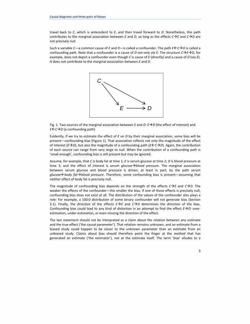
Let E D be the effect of interest, which may be strong, weak, or even precisely null. The marginal (‘crude’) association between E and D (of whatever magnitude) is due, in part, to the effect E D (Figure 1). Unfortunately, however, that arrow is not the only contributor to the marginal association.

Figure 1 also shows a variable C, which is antecedent to E (and therefore antecedent to D as well). By definition C E and C D, regardless of the magnitude of these effects. Recalling that causation is a forward association in time, the structure E C D does not depict causation between E and D because the path of arrows from E to D requires backward movement in time. Starting at E, we first


3

travel back to C, which is antecedent to E, and then travel forward to D. Nonetheless, this path contributes to the marginal association between E and D, so long as the effects C E and C D are not precisely null.

Such a variable C—a common cause of E and D—is called a confounder. The path E C D is called a confounding path. Note that a confounder is a cause of D not only via E. The structure C E D, for example, does not depict a confounder even though C is cause of E (directly) and a cause of D (via E). It does not contribute to the marginal association between E and D.

Fig. 1. Two sources of the marginal association between E and D: E D (the effect of interest) and E C D (a confounding path)

Evidently, if we try to estimate the effect of E on D by their marginal association, some bias will be present—confounding bias (Figure 1). That association reflects not only the magnitude of the effect of interest (E D), but also the magnitude of a confounding path (E C D). Again, the contribution of each source can range from very large to null. When the contribution of a confounding path is ‘small enough’, confounding bias is still present but may be ignored.

Assume, for example, that C is body fat at time 1; E is serum glucose at time 2; D is blood pressure at time 3; and the effect of interest is serum glucose blood pressure. The marginal association between serum glucose and blood pressure is driven, at least in part, by the path serum glucose body fat blood pressure. Therefore, some confounding bias is present—assuming that neither effect of body fat is precisely null.

The magnitude of confounding bias depends on the strength of the effects C E and C D. The weaker the effects of the confounder—the smaller the bias. If one of these effects is precisely null, confounding bias does not exist at all. The distribution of the values of the confounder also plays a role: For example, a 100:0 distribution of some binary confounder will not generate bias (Section 3.1). Finally, the direction of the effects C E and C D determines the direction of the bias. Confounding bias could lead to any kind of distortion in an attempt to find the effect E D: over‐estimation, under‐estimation, or even missing the direction of the effect.

The last statement should not be interpreted as a claim about the relation between any estimate and the true effect (‘the causal parameter’). That relation remains unknown, and an estimate from a biased study could happen to be closer to the unknown parameter than an estimate from an unbiased study. Claims about bias should therefore point the finger at the method that has generated an estimate (‘the estimator’), not at the estimate itself. The term ‘bias’ alludes to a

E

C

D


4

discrepancy between the theoretical result of a study at infinity and the causal parameter. Some writers consider “at infinity” as infinite replications of the study. We prefer to consider it as an infinite‐size version of the study.

3.1 Deconfounding

Most, if not all, of the methods to eliminate confounding bias are based on conditioning, which means (in its simplest form) restricting a variable to one of its values. Conditioning (denoted by a box) dissociates a “variable”—now just a value—from both its causes and its effects, because a value is not associated with any other variable. For example, rather than estimating the marginal association between E and D, we would estimate a conditional association—the association between E and D when the confounder C is restricted to C=c. Since the confounding path has been blocked (Figure 2, Diagram A), the only source of the conditional association is the effect E D.

Fig. 2. Conditioning (denoted by a box) dissociates a variable from its causes and its effects (denoted by two lines over incoming and outgoing arrows). After conditioning, confounding bias is eliminated (Diagrams A and B) and is either reduced or increased (Diagram C)

It is not always necessary to deconfound by conditioning on the confounder. A confounding path may sometimes be blocked by conditioning on an intermediary variable (I) along the path (Figure 2, Diagram B). That would not suffice, however, if the effect of the confounder is not exclusively mediated by the intermediary (Figure 2, Diagram C). In that case, conditioning on the intermediary might reduce, but not eliminate, confounding bias because one confounding path is still open (E C D). Whether bias will be reduced at all depends on the two paths by which C affects D (C I D and C D). If both of them deliver causation of D in the same direction, confounding bias will be reduced. Otherwise, the bias will actually increase, because the association of C with D will be strengthened, rather than weakened, after conditioning on I. Similar arguments apply to conditioning on an intermediary variable between C and E (C I E).

3.2 Deconfounding by restriction, stratification, or regression

Conditioning may be achieved by restricting the sample to people who share a single value of the confounder—for example, recruiting only women into the study. Alternatively, conditioning may be

E

C

D

E D

I C

E D

I C

Diagram A Diagram B Diagram C


5

achieved by stratification of the sample on the values of the confounder. If the confounder, C, is a categorical variable with k values, stratification will generate k estimates of the effect E D, one per each value (stratum) of C. Assuming no effect modification between E and C, all the estimates may be replaced with a single weighted average, which is a deconfounded estimator of the effect E D.

To remove confounding by several categorical variables, we may stratify on all of them simultaneously and compute a weighted average of as many estimates as we get (again, assuming no effect modification). Of course, as the number of strata increases, the number of stratum‐specific observations decreases and at some point the method will fail: reduction of confounding bias will cost too large of a variance. The method will also fail when we have to condition on continuous variables where stratification is practically impossible. In those cases, regression analysis usually substitutes for a simple weighted average. The variables are added to the right hand side of a regression model.

3.3 Deconfounding by randomization

A confounding path (E C D) may be eliminated by another method, besides conditioning on the confounder C, or on some intermediary on the path. Suppose that E has a cause, R, which is not a confounder, and that R and the confounder C are effect modifiers with respect to E (Figure 3, Diagram A). Suppose further that the effect C E is null for some value of R, say, R=1. If we restrict the sample to R=1 (condition on R), the confounder C will not be associated with E, and the confounding path will no longer exist (Figure 3, Diagram B).

Fig. 3. Deconfounding by conditioning on R, a modifier of the effect C E (Diagram A), assuming that the effect C E is null when R=1 (Diagram B)

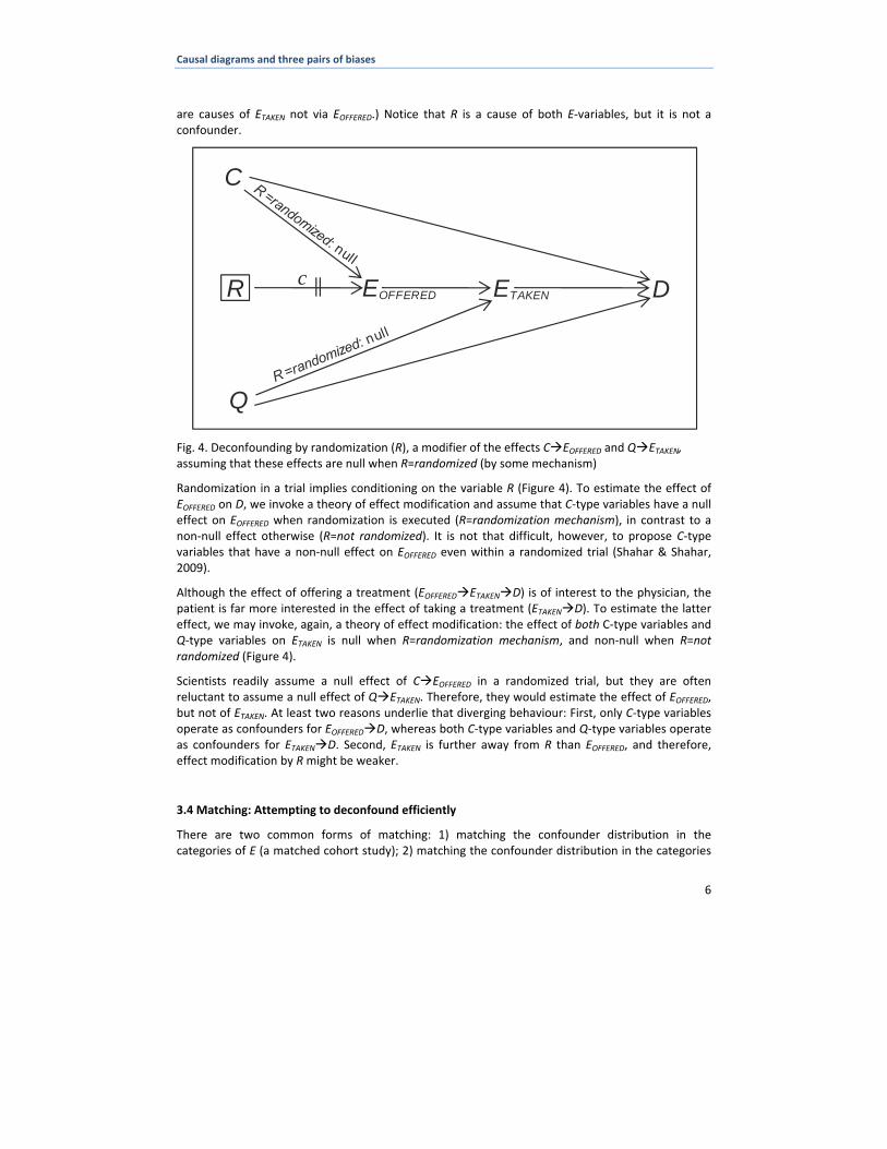
That method operates in a randomized trial (Figure 4). The first cause on the horizontal path is the randomization mechanism (R), which takes a value for each possible mechanism (e.g., a coin toss, a computer program), as well as one value for ‘not randomized’. R is a cause of the treatment offered, EOFFERED, because the probability of offering some treatment in a randomized study differs from that probability in a non‐randomized study. EOFFERED, in turn, is a cause of ETAKEN—the treatment actually taken by a patient—and ETAKEN is a cause of D.

Both E‐variables have other causes, too, some of which are also causes of D not via E (Figure 4). When the effect of interest is EOFFERED D, C‐type variables are confounders. When the effect of interest is ETAKEN D, both C‐type variables and Q‐type variables are confounders. (Q‐type variables

E

C

D

Diagram A Diagram B

R c

r

E

C

DR c


6

are causes of ETAKEN not via EOFFERED.) Notice that R is a cause of both E‐variables, but it is not a confounder.

Fig. 4. Deconfounding by randomization (R), a modifier of the effects C EOFFERED and Q ETAKEN, assuming that these effects are null when R=randomized (by some mechanism)

Randomization in a trial implies conditioning on the variable R (Figure 4). To estimate the effect of EOFFERED on D, we invoke a theory of effect modification and assume that C‐type variables have a null effect on EOFFERED when randomization is executed (R=randomization mechanism), in contrast to a non‐null effect otherwise (R=not randomized). It is not that difficult, however, to propose C‐type variables that have a non‐null effect on EOFFERED even within a randomized trial (Shahar & Shahar, 2009).

Although the effect of offering a treatment (EOFFERED ETAKEN D) is of interest to the physician, the patient is far more interested in the effect of taking a treatment (ETAKEN D). To estimate the latter effect, we may invoke, again, a theory of effect modification: the effect of both C‐type variables and Q‐type variables on ETAKEN is null when R=randomization mechanism, and non‐null when R=not randomized (Figure 4).

Scientists readily assume a null effect of C EOFFERED in a randomized trial, but they are often reluctant to assume a null effect of Q ETAKEN. Therefore, they would estimate the effect of EOFFERED, but not of ETAKEN. At least two reasons underlie that diverging behaviour: First, only C‐type variables operate as confounders for EOFFERED D, whereas both C‐type variables and Q‐type variables operate as confounders for ETAKEN D. Second, ETAKEN is further away from R than EOFFERED, and therefore, effect modification by R might be weaker.

3.4 Matching: Attempting to deconfound efficiently

There are two common forms of matching: 1) matching the confounder distribution in the categories of E (a matched cohort study); 2) matching the confounder distribution in the categories

EOFFERED

C

DR c ETAKEN

Q


7

of D (a matched case‐control study). Both methods try to remove confounding bias more efficiently—reduce the variance—than would have been achieved otherwise with a given sample size. In both cases, however, the saving of variance is not guaranteed and is not free. Extra effort must be paid.

Deconfounding with matching relies, in part, on a phenomenon called colliding (Section 4). We, therefore, defer the explanation until the end of the next section.

4. Colliding bias

Let E D be the effect of interest, and let C be a shared effect of E and D (Figure 5, Diagram A). The structure E C D does not depict causation between E and D, because the path of arrows from E to D via C requires backward movement in time. Starting at E, we first travel forward to C, and then travel backward to D, which is antecedent to C.

Fig. 5. The path E C D does not contribute to the marginal association between E and D (Diagram A). But conditioning on C (Diagram B) often contributes to the conditional association between the colliding variables E and D (denoted by a dashed line)

Furthermore, that path—unlike a confounding path—does not contribute to the marginal association between E and D, because a common effect (a future variable) does not induce an association between its causes (past variables). The path E C D is an innocent bystander; it does not deliver any bias.

Since the arrowheads in E C and D C ‘collide’ at C, the variables E and D are called ‘colliding variables’; C itself is called ‘a collider on the path E C D’. Note that a collider, just like a confounder, is a path‐specific term. A variable may be a collider on one path and not a collider on another. For example, if C is a cause of another variable, F (C F), then C is not a collider on the paths E C F and E D C F even though it is still a collider on the path E C D.

As we have seen, conditioning on a confounder removes confounding bias. In contrast, conditioning on a collider sometimes adds bias. After conditioning on C (Figure 5, Diagram B), the colliding variables E and D will be associated not only due to the effect E D, but also due to a newly‐formed association between them (E‐‐‐D). Consequently, the estimator contains a new type of bias—

E

C

D E

C

D

Diagram A Diagram B


8

colliding bias. How much bias will be added, and whether bias will be added at all, depends on several factors: the value to which C is restricted; effect‐modification between E and D on the probability ratio scale; and the type of post‐conditioning analysis (a weighted average, regression, or none). Unlike confounding bias, some rules that govern colliding bias depend on the scale and analysis by which effects are estimated.

Why does conditioning on a collider sometimes create an association between the colliding variables? (And why does a confounder create an association between its effects?) Formal proofs are available, but we will just provide intuitive explanations. Considering confounders first: Suppose that sex is a cause of both aspirin use and estrogen use (aspirin use sex estrogen use), such that the probability of taking each drug is higher in females than in males. If we know that Jordan takes aspirin, we may guess that baby Jordan was a girl, and therefore, we may also guess that “she” takes estrogen, too. The ability to guess estrogen use from aspirin use reflects a marginal association between the two variables.

Conditioning on a collider is a little more complicated. Suppose that vital status is an effect of two causes, aspirin use and statin use (aspirin use vital status statin use), such that the probability of vital status=alive is higher for users of either drug. If we know, for example, that Taylor did not take aspirin, that knowledge alone does not allow an informed guess about whether Taylor took a statin drug. There is no marginal association between the colliding variables. Nonetheless, an association will be created after conditioning on vital status. For example, if we also know that Taylor is alive (vital status=alive), we may now guess that Taylor took a statin drug.

Confounding bias is part of the causal structure over which we have no control. We can remove the bias, but we cannot make the arrows disappear. Colliding bias, however, is not part of causal reality. We create the bias by conditioning—a human decision that may be avoided. If that’s not feasible or possible, the bias can sometimes be removed by conditioning on other variables, as explained later.

4.1 Types and structures of colliding bias

Confounding bias takes a single causal structure: E C D. Colliding bias takes many forms, because the colliding variables are not always the cause‐and‐effect of interest. We describe, next, two types and several structures of colliding bias, and methods to avoid or remove it.

4.1.1 Sampling colliding bias

In one of the early examples of colliding bias, E was cholecystitis, D was diabetes, C was hospitalization status, and the effect of interest was cholecystitis diabetes. Both cholecystitis and diabetes are assumed to be causes of hospitalization. Colliding bias was inadvertently added by restricting the studies to hospitalized patients (Berkson, 1946)—that is, conditioning on hospitalization status. As a result, the conditional association between cholecystitis and diabetes was driven, at least in part, by a non‐causal component. The bias could have been avoided by ignoring hospitalization status in the sampling protocol.

The classical structure of colliding bias may be elaborated by adding an intermediary variable, I, between E and C (Figure 6, Diagram A). Although the pair of colliding variables is I and D—not E and D—colliding bias is still present, because the new association between I and D contributes to the association between E and D via the new path E I‐‐‐D. (Think of a dashed line on a path as an open


9

bridge that transmits associations from side to side in the absence of an arrow, or in addition to an arrow.)

Fig. 6. Colliding bias that is transmitted via an intermediary I (Diagram A) can be eliminated by conditioning on I (Diagram B), unless E affects C not only through I (Diagram C)

A case‐control study is prone to this structure of colliding bias. Let C be a binary variable that indicates whether a person is selected into a study (C=1) or not (C=0). In a case‐control study, the effect D C is typically strong, because people with the disease are much more likely to be sampled than their disease‐free counterparts. Since only sampled people (C=1) are actually studied in any research design, conditioning on C is inevitable.

All that it takes to turn C into a collider is an effect E C. Such an effect may be introduced, inadvertently, by a sampling decision. For example, if the effect of interest is weight (E) hip fracture (D), and weight (E) diabetes (I), selecting diabetic patients as controls (I C) will create the structure in Figure 6 (Diagram A). That unfortunate sampling decision will add a path of colliding bias: weight (E) diabetes (I)‐‐‐hip fracture (D).

As explained before, prevention is the best remedy: do not sample controls on the basis of diabetes status. Simply ignore the variable during selection. If the bias is already present, it may be removed by conditioning on diabetes status, the intermediary variable (Figure 6, Diagram B). That additional conditioning dissociates I from both E (denoted by two lines over the arrow) and D (denoted by the deletion of the dashed line)—thereby eliminating the path of colliding bias. If the effect of E on C is not exclusively mediated by I, the solution will fail (Figure 6, Diagram C).

Colliding bias in a case‐control study could take another form (Figure 7, Diagram A). Here, the colliding variable, Z, is a cause of E—not an effect of E. After inevitable conditioning on C (selection status), the newly formed path E Z‐‐‐D contributes to the conditional association between E and D. This structure will operate, for example, in a case‐control study of the effect of assisted living (E) on injury (D), if health insurance (Z) affects assisted living status and insured people are preferentially selected as controls. Again, the bias can be avoided by ignoring insurance status during control selection, or removed by conditioning on this variable (Figure 7, Diagram B).

Disease status in a cohort study follows selection into the cohort and cannot be a cause of selection status. Nonetheless, another type of collider could create sampling colliding bias. Let C indicate

E D

I


C

E D

I

C

E D

I

C


10

whether a cohort member is observed at the end of the study (C=1) or not (C=0). Since the final sample is restricted to C=1, conditioning on C is built into the design.

Fig. 7. Colliding bias in a case‐control study where Z, a cause of E, also affects selection (Diagram A). The bias can be removed by conditioning on Z (Diagram B).

Colliding bias would be present if E C and some cause of the disease, Z, is also a cause of C (Figure 8, Diagram A). For example, in a cohort study of health education (E) and lung function (D), health education (E) is a cause of loss to follow‐up (perhaps via interest in continued participation), and Z might be ‘place of residence’—a cause of lung function (D), say, via amount of pollutants in the lungs, and also a cause of loss to follow‐up (C). Again, the bias can be removed by conditioning on Z, which would block the path E‐‐‐Z D (Figure 8, Diagram B). Notice that colliding bias will also be created if E and C are associated due to a common cause, rather than E C.

Fig. 8. Colliding bias in a cohort study where E affects ‘censoring status’ (C) and Z is a common cause of C and D (Diagram A). The bias can be removed by conditioning on Z (Diagram B).

4.1.2 Analytical colliding bias

Colliding bias might arise during data analysis by a deliberate decision to condition on a variable. Whether colliding bias will be added depends on the causal structure and the group of variables that is chosen for conditioning (in addition to previously mentioned factors).

E D

Z

Diagram A Diagram B

C

E D

Z

C

E D

Z

Diagram A

C

E D

Z

Diagram B

C


11

Figure 9 (Diagram A) shows a ‘crown‐like’ structure for a study of the effect of E on D. Two paths connect E with D: The path we wish to estimate (E D), and a path with two colliders, C1 and C2, neither of which is an effect of E or D (E X C1 Y C2 Z D). Since there are no confounders, the marginal association between E and D is an unbiased estimator of the effect E D. No deconfounding is needed.

Unnecessary conditioning on C1 (Figure 9, Diagram B) will create an association between the colliding variables X and Y, but will not add colliding bias because C2, the other collider, blocks the new path (E X‐‐‐Y C2 Z D). Conditioning on C2 alone will not add bias either. And in all cases, conditioning on a collider on a path between E and D—or even on several colliders—will not add colliding bias so long as at least one collider on that path remains intact. Colliding bias will arise only when we condition on every collider on a path (Figure 9, Diagram C).

But why would anyone condition on C1 and C2 in the first place?

The answer is simple. Worried about confounding bias, many scientists choose covariates (variables for conditioning) by informal verbal arguments about ‘potential confounders’, or by statistical procedures such as stepwise regression. A common method is the ‘change‐in‐estimate’ rule, according to which conditioning on a variable is needed, if the estimated association changes after conditioning. All of these methods fail to distinguish between confounders and colliders. Therefore, they are just as likely to add colliding bias as they are to remove confounding bias. To remove confounding in a rationalized way, variables should be displayed in a causal diagram and conditioning should follow the rules of open and blocked paths.

Fig. 9. The effect E D can be estimated by their marginal association (Diagram A). Unnecessary conditioning on the collider C1 does not add bias (Diagram B), but unnecessary conditioning on both C1 and C2 opens a new path and adds colliding bias (Diagram C)

E

C1

D

Diagram B

X Z

C2

Y

E

C1

D

X Z

C2

Y

Diagram A

E

C1

D Diagram C

X Z

C2

Y


12

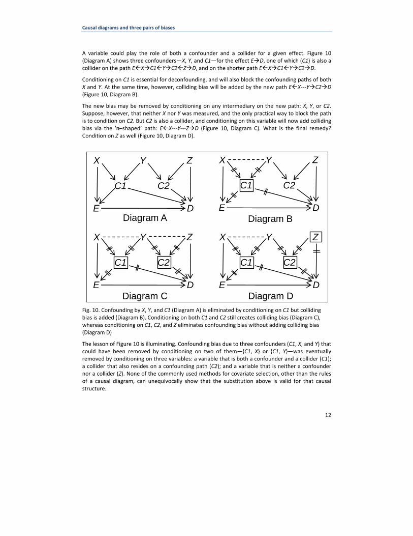
A variable could play the role of both a confounder and a collider for a given effect. Figure 10 (Diagram A) shows three confounders—X, Y, and C1—for the effect E D, one of which (C1) is also a collider on the path E X C1 Y C2 Z D, and on the shorter path E X C1 Y C2 D.

Conditioning on C1 is essential for deconfounding, and will also block the confounding paths of both X and Y. At the same time, however, colliding bias will be added by the new path E X‐‐‐Y C2 D (Figure 10, Diagram B).

The new bias may be removed by conditioning on any intermediary on the new path: X, Y, or C2. Suppose, however, that neither X nor Y was measured, and the only practical way to block the path is to condition on C2. But C2 is also a collider, and conditioning on this variable will now add colliding bias via the ’shaped–ח’ path: E X‐‐‐Y‐‐‐Z D (Figure 10, Diagram C). What is the final remedy? Condition on Z as well (Figure 10, Diagram D).

Fig. 10. Confounding by X, Y, and C1 (Diagram A) is eliminated by conditioning on C1 but colliding bias is added (Diagram B). Conditioning on both C1 and C2 still creates colliding bias (Diagram C), whereas conditioning on C1, C2, and Z eliminates confounding bias without adding colliding bias (Diagram D)

The lesson of Figure 10 is illuminating. Confounding bias due to three confounders (C1, X, and Y) that could have been removed by conditioning on two of them—{C1, X} or {C1, Y}—was eventually removed by conditioning on three variables: a variable that is both a confounder and a collider (C1); a collider that also resides on a confounding path (C2); and a variable that is neither a confounder nor a collider (Z). None of the commonly used methods for covariate selection, other than the rules of a causal diagram, can unequivocally show that the substitution above is valid for that causal structure.

E

C1

D

X Z

C2

Y

Diagram A

E

C1

D Diagram C

X Z

C2

Y

E

C1

D Diagram B

X Z

C2

Y

E

C1

D Diagram D

X Z

C2

Y


13

4.1.3 Some other structures of colliding bias

There are many other structures of colliding bias, three of which are shown in Figure 11. Let I be an intermediary between E and D (E I D), and let C be a common effect of E and I (E C I). Unnecessary conditioning on C contributes to the association between E and I (Diagram A). As a result, two components make up the conditional association between E and D: E I D (the effect of interest) and E‐‐‐I D (colliding bias). No simple remedy is available.

In Diagram B of Figure 11 the collider, C, is a cause of E and a common effect of a confounder (A) and a cause of E which is not a confounder (B). Conditioning on the collider adds bias through the path E B‐‐‐A D, which can be removed by conditioning on B or A. (In fact, conditioning on A alone would remove confounding bias without adding colliding bias.)

Fig. 11. Three structures of colliding bias: unnecessary conditioning (Diagram A); conditioning on an intermediary on a confounding path (Diagram B); conditioning on an effect of D when E and D collide at C, but E affects C only through D (Diagram C)

A special type of colliding bias is shown in Diagram C of Figure 11. The structure is simple: D is a cause of C, and E is also a cause of C (albeit only via D). Therefore, D and E collide at C (unless E D C is a precisely null effect). We may call this structure ‘uni‐path’ colliding bias, to distinguish it from colliding via separate paths (‘bi‐path’ colliding bias). Note that if E affects C not only through D (E C), the structure is, again, ‘bi‐path’ colliding bias. (There is no additional ‘uni‐path’ bias.)

The causal structure in Diagram C of Figure 11 depicts a classical case‐control study in which controls are sampled from disease‐free people at a fixed follow‐up time (the ‘cumulative’ design). As we have seen, disease status (D) affects selection status (C), and conditioning on C is inevitable because only sampled people are studied. Does every case‐control study contain some uni‐path colliding bias, unless the effect E D is precisely null?

The answer depends on the measure of effect. If the effect is estimated by a probability ratio or a probability difference, colliding bias is indeed present (Figure 11, Diagram C). But if the effect is

E

C

D I

Diagram A Diagram B

E

A

B

C D

Diagram C

E C D


14

estimated by an odds ratio, the dashed line E‐‐‐D is not created (proof omitted). Therefore, odds ratios should be computed from a case‐control study, unless the bias in probability measures is small. When the sampling fraction of controls is known, probability measures can be computed with no colliding bias, but the causal diagram is different.

The same structure (Figure 11, Diagram C) also describes a cross‐sectional study in which the disease of interest (D) affects vital status (C). Since only alive people are typically studied, conditioning on C is built into the design, and some uni‐path colliding bias is present. Consider, for instance, a cross‐sectional study of the effect of genotype (E) on myocardial infarction (D), which, in turn, affects vital status (C). Unless the effect genotype (E) myocardial infarction status (D) vital status (C) is precisely null, some colliding bias is present—whenever probability ratios are estimated. What is the remedy (when the bias isn’t small)? Estimate the odds ratio, as in a case‐control study.

It is interesting to compare the structure E D C with the structure C E D, which was mentioned before (Section 3): Changing the role of C from an effect of E and D to a cause of E and D turns C from a ‘uni‐path collider’ into a ‘pseudo‐confounder’. But conditioning on a ‘pseudo‐confounder’—unlike conditioning on a ‘uni‐path collider’— will not add bias, regardless of which measure of effect is computed. It will, however, unnecessarily increase the variance of the estimated effect.

4.2 Beneficial colliding

In Section 3.4, we mentioned that deconfounding with matching relies, in part, on colliding. In fact, to match means to create a collider by sampling, and to condition on that variable. Interestingly, what has been called colliding bias so far, will prove helpful in the context of deconfounding.

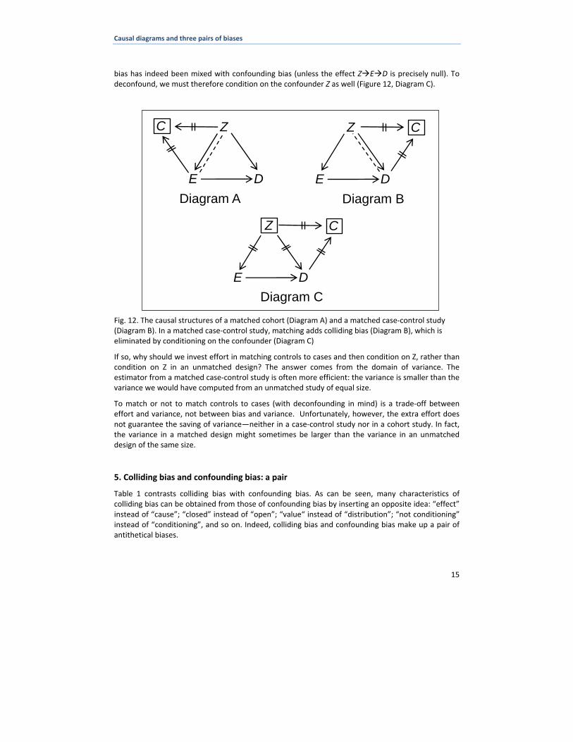
Figure 12 (Diagram A) shows the causal structure of a matched cohort. The effect of interest is E D; Z is a confounder on which we match; and C denotes selection status. Matching the distribution of Z in the categories of E means that both E and Z affect selection status (C). Recall that conditioning on C is a feature of every study, because only selected people are studied.

At first glance, it seems that the situation is worse because colliding bias (E‐‐‐Z D) has been added to confounding bias (E Z D). Not so. Although matching has contributed to the association between E and Z, that addition counteracted the contribution of Z E—nullifying the overall association between the two variables. Indeed, as we know E and Z are not associated after matching. Since the ‘associational sum’ of Z E and Z‐‐‐E is null, bias has been removed.

Thinking back for a moment, we have seen three methods to dissociate a confounder Z from E: conditioning on Z (or on an intermediary on the path), which prevents an arrow from creating an association; conditioning on a modifier such that the effect Z E is null (randomization); and conditioning on a collider, which nullifies the ‘associational sum’ of Z E and Z‐‐‐E (matching in a cohort).

The situation is a little more complicated in a matched case‐control study, where we match controls to cases on Z (Figure 12, Diagram B). Analogous to a matched cohort, matching contributes to the association between Z and D, and the two variables are no longer associated: the ‘associational sum’ is null. But in this case the overall null association is composed from three paths, not two: Z D; Z‐‐‐D; and Z E D. Therefore, the ‘sum’ of Z D and Z‐‐‐D alone is not null, which means that colliding


15

bias has indeed been mixed with confounding bias (unless the effect Z E D is precisely null). To deconfound, we must therefore condition on the confounder Z as well (Figure 12, Diagram C).

Fig. 12. The causal structures of a matched cohort (Diagram A) and a matched case‐control study (Diagram B). In a matched case‐control study, matching adds colliding bias (Diagram B), which is eliminated by conditioning on the confounder (Diagram C)

If so, why should we invest effort in matching controls to cases and then condition on Z, rather than condition on Z in an unmatched design? The answer comes from the domain of variance. The estimator from a matched case‐control study is often more efficient: the variance is smaller than the variance we would have computed from an unmatched study of equal size.

To match or not to match controls to cases (with deconfounding in mind) is a trade‐off between effort and variance, not between bias and variance. Unfortunately, however, the extra effort does not guarantee the saving of variance—neither in a case‐control study nor in a cohort study. In fact, the variance in a matched design might sometimes be larger than the variance in an unmatched design of the same size.

5. Colliding bias and confounding bias: a pair

Table 1 contrasts colliding bias with confounding bias. As can be seen, many characteristics of colliding bias can be obtained from those of confounding bias by inserting an opposite idea: “effect” instead of “cause”; “closed” instead of “open”; “value“ instead of “distribution”; “not conditioning” instead of “conditioning”, and so on. Indeed, colliding bias and confounding bias make up a pair of antithetical biases.

Diagram A

E D

Z

Diagram B

C

E D

Z C

E D

Z

Diagram C

C


16

Confounding bias Colliding bias

Main feature Common (shared) cause of two variables

Common (shared) effect of two variables

Causal structures Single: E C D

Several. For example: E C D (‘bi‐path’) E C L D (‘bi‐path’) E D C (‘uni‐path’)

Type of path Associational (open) Blocked (closed) Presence of bias Not conditioning on one of the

confounders (of the relevant association)

Conditioning on all of the colliders (on the relevant path)

Magnitude of bias depends on:

1. the distribution of C 2. the magnitude of C’s effects

on E and D

1. the value of C 2. the magnitude of effect

modification between the causes of C (‘bi‐path’ bias)

3. the magnitude of E’s effect on C (‘uni‐path’ bias)

4. the measure of effect (‘uni‐path’ bias)

Removal of bias (primary method)

Conditioning on all confounders (of the relevant association)

Not conditioning on at least one collider (on each relevant path)

Removal of bias (secondary method)

Conditioning on an effect of the confounder (on the confounding path), rather than conditioning on the confounder

Conditioning on a cause of a collider (on the colliding path), in addition to conditioning on the collider

Table 1. Antithetical characteristics of confounding bias and colliding bias

6. Effect‐modification bias

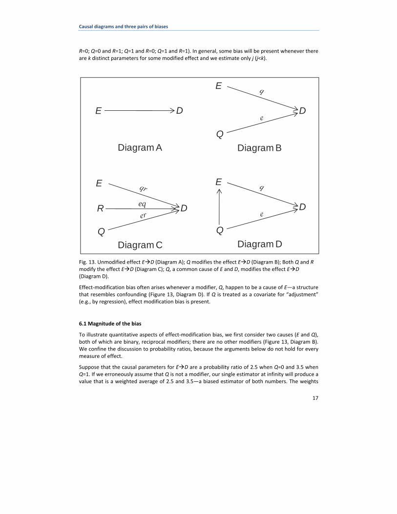
As we saw in Section 2, the effect E D could be uniform for any value of any other cause of D (Figure 13, Diagram A), or could vary across the values of another cause (Figure 13, Diagram B), two other causes (Figure 13, Diagram C), or any number of causes. The reciprocal phenomenon of a varying effect was called effect modification (Section 2).

If only one binary modifier exists (Q=0; Q=1), the effect E D is described by two causal parameters: one parameter when Q=0, and another when Q=1. If we erroneously assume a single causal parameter (Figure 13, Diagram A), our estimator is obviously biased. A theoretical result of the study at infinity will not deliver two parameters. Since the bias arose from failure to estimate a modified effect (Shahar, 2007), it is called ‘effect‐modification bias’.

Effect‐modification bias will also be present if several variables modify the effect E D, yet only some of them are considered as modifiers (Shahar & Shahar, 2010a). In the simplest example, both Q and R are modifiers (Figure 13, Diagram C), but we assume that the effect of E on D varies only according to the value of Q (Figure 13, Diagram B). If E, Q, and R are all binary variables, we mistakenly estimate two causal parameters for the effect E D (Q=0; Q=1), instead of four (Q=0 and


17

R=0; Q=0 and R=1; Q=1 and R=0; Q=1 and R=1). In general, some bias will be present whenever there are k distinct parameters for some modified effect and we estimate only j (j<k).

Fig. 13. Unmodified effect E D (Diagram A); Q modifies the effect E D (Diagram B); Both Q and R modify the effect E D (Diagram C); Q, a common cause of E and D, modifies the effect E D (Diagram D).

Effect‐modification bias often arises whenever a modifier, Q, happen to be a cause of E—a structure that resembles confounding (Figure 13, Diagram D). If Q is treated as a covariate for “adjustment” (e.g., by regression), effect modification bias is present.

6.1 Magnitude of the bias

To illustrate quantitative aspects of effect‐modification bias, we first consider two causes (E and Q), both of which are binary, reciprocal modifiers; there are no other modifiers (Figure 13, Diagram B). We confine the discussion to probability ratios, because the arguments below do not hold for every measure of effect.

Suppose that the causal parameters for E D are a probability ratio of 2.5 when Q=0 and 3.5 when Q=1. If we erroneously assume that Q is not a modifier, our single estimator at infinity will produce a value that is a weighted average of 2.5 and 3.5—a biased estimator of both numbers. The weights

Q

D

Diagram B

E

Diagram C

E

D

Diagram A

Q

D

E

R eq

Q

D

Diagram D

E


18

are a function of the effect Q D and the distribution of Q in the study. In general, the magnitude of the bias is inversely related to the weight: the larger the weight for some value of a missed modifier, the smaller the bias for that value. For instance, if the weights for 2.5 and 3.5 were 0.1 and 0.9, respectively, the biased average (3.4) is closer to 3.5 than to 2.5. Of course, the magnitude of the bias also depends on the magnitude of effect modification between E and Q. For example, if the causal parameters were 2.6 and 2.7, effect modification bias will be minimal for both Q=0 and Q=1, regardless of the weights in our biased estimator.

We consider, next, three causes (E, Q, and R) and similar basic assumptions: binary variables and no other modifiers (Figure 13, Diagram C). The effect of interest, E D, is estimated again by probability ratios.

Table 2. Effect‐modification bias when Q and R modify the effect E D, yet only Q is assumed to be a modifier

Assuming an infinite–size study, Table 2 shows the probability of D=1 for every combination of the values of E, Q, and R, as well as four causal parameters. Although three of the four parameters are identical, effect modification by Q and R is evident because one parameter is different (E D when Q=1 and R=1). If we erroneously assume that only Q is a modifier (Figure 13, Diagram B), only two estimators exist: one estimator for Q=0 and another for Q=1. Each estimator assumes that the value of R makes no difference—for example, the effect E D when Q=1 and R=1 is assumed to be identical to the effect E D when Q=1 and R=0 (Table 2, right column). Given our false assumption, how much bias is present?

As before, ignoring the modifier R means taking a weighted average of two causal parameters (over R=0 and R=1). When Q=0, that’s a weighted average of 2 and 2, and no bias is present, regardless of the weights (Table 2). When Q=1, however, the probability ratio (p) in an infinite‐size study is a weighted average of 2 and 3, which is constrained in the interval [2, 3]. The exact value of p depends on the weights. Again, the larger the weight for some value of R, the smaller the bias for that value.

6.2 Is there effect‐modification bias?

Figure 14 shows that E affects D by two paths: one path via an intermediary variable I and another ‘direct’ path. The diagram also shows another cause, Q, and effect modification between E and Q,

E

Q

R

Pr (D=1)

E D 4 causal parameters (probabaility ratios)

E D 2 estimators

(probability ratios) 0 0 0 0.1 1 0 0 0.2 2 2 0 0 1 0.2 1 0 1 0.4 2 2 0 1 0 0.3 1 1 0 0.6 2 2 ≤ p ≤ 3 0 1 1 0.3 1 1 1 0.9 3 2 ≤ p ≤ 3


19

but the symbol of effect modification is displayed only on the ‘direct’ arrows (E D, Q D). Suppose we assume that Q is not a modifier and we estimate the effect of E on D, ignoring Q. Is there effect‐modification bias?

Fig. 14. The direct effect E D is modified by Q, but the indirect effect (via I) is not

To answer the question, we should first state which effect of E is of interest: the indirect effect via I, the ‘direct’ effect, or the total effect? Of these, only two are modified by Q: the ‘direct’ effect and the total effect (because the modified ‘direct’ effect contributes to the total). Nonetheless, there is no modification of E I D: the effect of E via this path is uniform for all values of Q. Consequently, effect‐modification bias is present if we estimate the total effect or the ‘direct’ effect, but is absent if we estimate the indirect effect.

Figure 14 shows that the effect Q D is different for at least one value of E, yet the effect E I D does not vary according to the value of Q. Does it mean that reciprocity of effect modification does not hold? No. Reciprocity still holds for the total effect of each cause.

To summarize, effect modification between two or more causes of D implies effect modification of at least one path between each variable and D, and effect modification of the variable’s total effect (ignoring theoretical, precise cancellations). It does not imply effect modification of every path by which a variable affects D. By the same token, a claim of effect‐modification bias should specify the relevant path(s).

We conclude this section with an interesting question: What are the consequences of assuming effect modification when it is absent? For example, what happens if we mistakenly assume that a binary variable, Q (Q D) modifies the effect E D and unnecessarily substitute two estimators for one?

As far as effect‐modification bias is concerned, no harm was done: both estimators are unbiased. But they are inefficient. Assuming no other reason to condition on Q (and no colliding bias), the variance has increased with no return in reduced bias or reduced effort. Other times, some effect‐modification bias may be traded for variance: we may ignore a modified effect and accept a small bias—in return for reduced variance.

E

I

Dq

Q

e


20

7. Causal‐pathway bias

Figure 15 shows three paths by which E affects D: one path via I; another via J; and a third, direct arrow. The ‘direct’ path, which was mentioned in Section 6.2, is not a direct effect, but simply serves as summary notation for all other paths of causation.

Fig. 15. E affects D via I; via J; and via all other paths (denoted by a direct arrow)

We may wish to estimate several kinds of effects of E on D (Table 3): the total effect (first row); the effect by all paths except via J (second row); the effect by all paths except via I (third row); and the ‘direct’ effect (last row).

Table 3. Path(s) of interest and examples of causal‐pathway bias

Causal‐pathway bias will operate whenever there is a mismatch between the path(s) we actually estimate and the path(s) we wish to estimate. The mismatch might result from excluding a path of interest, or from including a path that is not of interest. A path will be excluded if it is blocked (for example, by conditioning on an intermediary); a path will be included if it remains intact.

The right column of Table 3 shows examples of causal‐pathway bias. For instance, the bias will be present if we are interested in the total effect of E on D (first row) and we mistakenly condition on I. Likewise, the bias will be present if we are interested in the ‘direct’ path (last row), and we fail to condition on both I and J. The magnitude of causal‐pathway bias depends the magnitude (and

Path(s) of interest Examples of causal‐pathway bias E I D E D E J D

Conditioning on I, J, or both

E I D E D

Conditioning on I, not conditioning on J, or both

E D E J D

Conditioning on J, not conditioning on I, or both

E D Not conditioning on I and J

E

I

D

J


21

direction) of the effect via the path(s) that are mistakenly blocked, or remain open. (In principle, multiple mistakes could add up to no or little bias.)

7.1 The placebo effect

The attempt to block the so‐called placebo effect is a classical example of an attempt to remove causal‐pathway bias. Figure 16 (Diagram A) shows some elements of a randomized trial (Section 3.3) along with the ‘placebo path’ between EOFFERED and D.

If we wish to estimate the total effect of EOFFERED, we should consider, again, effect‐modification between B and E. Notice that when B=1 (blinding), the ‘direct’ path is also the total effect, because the placebo path should not exist. But when B=0 (no blinding), the total effect is the sum of the ‘direct’ path and the placebo path. Therefore, a blinded trial contains causal‐pathway bias for the total effect in the absence of blinding.

Fig. 16. The placebo path in a randomized trial (Diagram A); Removal of causal‐pathway bias when we estimate the ‘direct’ effect EOFFERED D (Diagram B)

EOFFERED

B

DR

e ‘A belief’

EOFFERED DR

‘A belief’

Diagram A

Diagram B


22

In a simple case, EOFFERED takes three values: offering of a drug, offering a placebo pill, or offering neither. What a patient believes to have taken is assumed to affect the outcome, D (if he also believes that taking the drug will help more than taking placebo, or more than taking nothing). That is the placebo effect, which may be negligible for some outcomes and strong for others. If the placebo effect is not precisely null, EOFFERED affects D not only ‘directly’, but also via the ‘belief’ variable (Figure 16, Diagram A).

We may therefore consider at least two kinds of effects of EOFFERED: the total effect and the ‘direct’ effect. Since the variable takes three values, there are three causal contrasts: drug vs. placebo; drug vs. nothing; and placebo vs. nothing.

Randomized trials typically try to estimate the ‘direct’ effect of EOFFERED for the contrast between offering a drug and offering placebo. Assuming that the placebo effect is not negligible, the placebo path should be blocked to remove causal‐pathway bias. As we saw before, a path may be blocked by a number of methods, one of which is built on the idea of effect modification. That method is chosen in a double‐blinded randomized trial (Figure 16, Diagram B).

The variable B indicates whether blinding is part of the protocol (B=1) or not (B=0). To block the placebo path, we assume that B modifies the effect EOFFERED A belief, such that the effect is null when blinding is executed (and not null in non‐blinded studies). Of course, our theory of a null effect, given blinding, might not be true. For example, the presence or absence of side effects might cause patients to believe that they know what they took.

Which of the two types of total effect is of greater interest: with blinding or without? Regulators care about the first type (total effect=’direct’ path), and they are interested only in the contrast between offering a drug and offering a placebo pill. Physicians and patients care about the second type (total effect=’direct’ path + placebo path) and about the contrast between offering a drug and not offering it. There are two reasons for the latter preference. First, physicians don’t usually blind their patients to the treatment they offer them, so the placebo path is part of the effect in daily medical practice. Second, physicians don’t usually choose between offering a drug and offering placebo, but between offering and not offering a drug. From that point of view, a placebo‐controlled, blinded trial contains causal‐pathway bias, whereas an open trial of a drug vs. no drug does not. As its name implies, the bias is tied to the causal path(s) of interest.

7.2 ‘Over‐adjustment’

Perhaps the most common type of causal‐pathway bias arises from conditioning on an intermediary between E and D—when the total effect is of interest (Table 3, first row). For example, we wish to estimate the total effect of estrogen use (E) at time 1 on coronary heart disease (D) at time 2, yet we condition on the blood concentration of estrogen (I) at an interim time. If the effect E I D is not precisely null, some causal‐pathway bias is present because a path of interest has been blocked. If instead, we wish to estimate the effect of estrogen use on coronary heart disease not via the blood concentration of estrogen, failure to condition on that variable will lead to causal‐pathway bias.

Causal‐pathway bias due to conditioning on an intermediary is often called ‘over‐adjustment’, a poorly standardized term (Schisterman et al., 2009). Other kinds of mistaken conditioning may also be called ‘over‐adjustment’: conditioning that increases the variance with no return; conditioning that creates colliding bias; and ‘adjustment’ that leads to effect‐modification bias. Sometimes, ‘over‐


23

adjustment’ from one point of view may be justified as an intentional trade‐off between two types of bias.

7.3 Relation to other biases

Trying to remove causal‐pathway bias, we might sometimes remove, and sometimes add, other biases. Figure 17 shows four examples. In Diagrams A, B, and C, the effect of interest is the ‘direct’ path E D. In Diagram D, it is the horizontal path E J D. Therefore, in all four examples we condition on the intermediary, I, to remove causal‐pathway bias.

Fig. 17. Consequences of removing causal‐pathway bias: confounding bias removed (Diagram A); colliding bias removed (Diagram B); colliding bias added (Diagrams C and D)

In Diagram A, removal of causal‐pathway bias has also removed confounding bias, whereas in Diagram B, removal of causal‐pathway bias has also removed colliding bias (due to conditioning on C). On the other hand, in Diagrams C and D the attempt to remove causal‐pathway bias has resulted in colliding bias.

Diagram B

E D

Diagram A C

E D J

I

I

E D

I

C

E D

Diagram C Z

I

Diagram D


24

8. Causal‐pathway bias and effect‐modification bias: a pair

Table 4 contrasts causal‐pathway bias with effect‐modification bias. As can be seen, the two may be considered a second pair of antithetical biases.

Effect‐modification bias Causal‐pathway bias Main feature Failure to consider

modification of an effect Failure to consider path(s) of an effect

Causal structure Multiple causes with modification. For example, E D Q D R D

A single cause with multiple paths. For example, E D E I D E J D

Type of path(s) Modified causation Causation Presence of bias 1. Not conditioning (mistakenly)

on a modifier 2. Conditioning on a modifier and (mistakenly) taking a weighted average across its values

1. Not conditioning (mistakenly) on an intermediary

2. Conditioning (mistakenly) on an intermediary, regardless of whether a weighted average is taken

Magnitude of bias depends on:

Magnitude of effect modification

Magnitude of effect

Removal of bias

Conditioning on modifiers Conditioning (or not conditioning) on intermediaries

Table 4. Antithetical characteristics of effect‐modification bias and causal‐pathway bias

9. Information bias

A value of a variable is an unknown value of a property of an object, such as a person’s height. When estimating the effect E D, we do not know, and cannot know, the values of E and D. Their true values remain missing forever, and so are the values of modifiers, confounders, colliders, and intermediaries on a path. All that we can do in science is to replace each variable of interest with another variable that is assumed to provide the missing information (Shahar, 2009). That inevitable substitution may be called imputation, because imputation in statistics means replacing a missing value (Shahar & Shahar, 2010c). To distinguish between a variable of interest and its imputed version, we’ll denote the latter by the subscript I—for ‘imputed’. Note that EI, DI and all other imputed variables exist at the moment at which the estimated effect is computed, not sooner (Shahar & Shahar, 2009).

Information bias is present whenever the association we estimate—using imputed variables—differs from the association we wish to estimate. The bias arises because imputed variables are not exact copies of the variables they replace.


25

9.1 Imputation by ‘measurement’

Figure 18 shows a simple example where EI, DI, and CI, are effects of the variables E, D, and C, respectively. The ‘direct’ path between a variable and its imputation usually indicates ‘measurement’. As explained elsewhere, however, that single arrow abbreviates a far more elaborated causal structure (Shahar & Shahar, 2010c).

Fig. 18. Information bias is present if the association between EI and DI after conditioning on CI differs from the association between E and D after conditioning on C

Since C is a confounder, conditioning on C is required, and the effect of interest should be estimated by the conditional association between E and D. In practice, however, we estimate the association between EI and DI (not E and D), after conditioning on CI (not C). If the value produced by the estimator at infinity differs from the causal parameter, information bias is present. Unbeknown to us, information bias might be large, small, or even absent, depending on the similarity between imputed variables and the variables they replace.

An imputed version of a variable differs from the original variable in part due to indeterministic causation (Popper, 1988; Shahar & Shahar, 2011) and in part due to other causes of the former, such as measurement method (not shown in Figure 18). Choosing a standardized measurement of some variable, say E, means conditioning on the variable ‘measurement method’. We assume effect modification between E and ‘measurement method’, such that the value of EI better resembles the value of E when one particular method is used.

9.2 Imputation using a derived variable

Whenever imputation by ‘measurement’ is not feasible or possible, the values of an imputed variable, say AI, may be obtained from other variables, say XI and YI, in a two‐step process: First, we assume that the values of some derived variable, denoted D, which are created from the values of X and Y, provide information on the unknown values of A. Second, we obtain information on the unknown values of D. Assuming that the first step was valid, the variable DI (the imputed version of D) is entitled to be called AI. If the first step is not valid, the imputation is useless (Section 10.1).

E

C

D

CI

EI DI


26

But why would the values of one variable, say X, provide information on the values of another, say A, when X is not a measurement of A?

The answer is simple: because the two variables are associated by some mechanisms: X is a cause of A; A is a cause of X; X and A share a common cause; or we condition on all colliders on a path between X and A. As we saw, a non‐null association means that the value of one variable provides information on the value of another.

Imputing the values of A using a derived variable, D, requires more than non‐null associations between A and the makers of D. We must also choose a function that will specify how the values of D are related to its makers (Shahar & Shahar, 2010c). If D is derived from just one variable, X, the function may be as simple as “If X=x, then D=x”. Obviously, if D is derived from two variables or more, the function would be more complicated.

Figure 19 shows an example. The unknown values of body surface area (A) are imputed from height (X) and weight (Y), which are assumed to be associated with body surface area (A) due to a gene (G)—a common cause of all three variables. As before, the values of XI and YI are obtained by ‘measurements’ (X XI and Y YI).

Fig. 19. The values of DIX,Y substitute for the unknown values of body surface area (A), relying on the

unknown values of height (X) and weight (Y)

Notice some new notation in Figure 19. First, the derived variable was labelled DX,Y to indicate its makers. Second, the choice of one derivation function means conditioning on the universe of all functions (denoted by F). Third, the arrows into DX,Y were drawn in the mathematical notation of ‘imply’, because theoretical derivation of the unknown values of DX,Y from the unknown values of X and Y is not causation (Shahar & Shahar, 2011). Imputation, in contrast, is a causal process that includes a choice of some computation program (denoted by P). For example, the values of XI and YI are keyed onto a calculator, and the value of DI

X,Y appears on the display.

About half a dozen functions have been proposed for the imputation of body surface area from height and weight, most of which take the form f(X,Y)=kXmYn. Indeed, the biggest challenge of imputation by a derived variable is often the choice of the function. That choice may be based on mathematical constraints, other theories, or an empirical method.

Imputation through a derived variable is also used when the values of a variable, A, were measured in some people, but not in others—a problem of missing data in the traditional sense. In that case the function is chosen, in part, by empirical means. For example, we may fit a linear regression

DX,Y

F

XI

YI

DI

X,Y

G

X

Y

P A


27

model of AI (as obtained by ‘measurement’) on XI,YI, and ZI to the non‐missing part of the sample, and then use the regression equation to impute the missing values: AI=DI

X,Y,Z=β0+β1XI+β2YI+β3ZI. Eventually, some of the unknown values of A are imputed by ‘measurement’ and some by a derived variable.

9.3 Invalid imputations

A derived variable, D, cannot substitute for A when its makers have null associations with A. But there are several other situations in which imputation by derivation is invalid. First, we should not impute the cause of interest from the effect of interest and vice versa. Obviously, the derivation itself creates an association between the imputed versions of the two variables.

Second, we should not impute an effect of the cause of interest using a variable that is not associated with that cause (ignoring some exceptions of precisely null effects). For example, Q should not be used to impute D if the structure is E D Q, because the association between E and Q is null (D is a collider), regardless of the magnitude of the effect E D.

Third, a variable should not be used in an imputation if conditioning on this variable is required to estimate the effect of interest. A variable cannot play a dual role in a single estimator (e.g., appear twice in linear regression): either it is used for imputation or it is used for conditioning (Shahar & Shahar, 2010c). (Conditioning, as we saw, might be needed to remove some other bias.)

Figure 20 (Diagram A) shows an example of imputation when conditioning is required to estimate the effect E Y. The values of DI

C (imputation from C) replace the unknown values of E, the cause of interest (Diagram A). But conditioning on C is required to block the confounding path. Unless that path can be blocked by some other means (Diagram B), the imputation is invalid (Diagram A).

Fig. 20. The values of DIC substitute for the unknown values of E. The imputation is not valid

(Diagram A), unless the confounding path due to C can be blocked without conditioning on C (Diagram B).

Consider, for instance, a study of the effect, at infancy, of exposure to respiratory viruses (E) on airway obstruction 10 years later (Y). That exposure may be imputed by the binary variable ‘day‐care attendance’ (C), assuming that the causal parameter for the effect day‐care attendance (C) exposure to respiratory viruses (E) is not null. The imputation is, of course, imprecise because a

DI

C P

E

C

Y E

I C

Y

DI

C P

Diagram A Diagram B

CI CI


28

binary variable substitutes for a continuous property (‘viral load’). But it is a priori invalid if day‐care attendance is a confounder (exposure to respiratory viruses (E) day‐care attendance (C) airway obstruction (Y)), and conditioning on that variable is needed. Nonetheless, if the magnitude of the confounding path is small, the imputation may be justified as a trade‐off: small confounding bias is tolerated in return for reduced effort (which would have been invested in imputing ‘viral load’ by other means).

9.4 Undesired paths between imputed variables

Sometimes, the cause of interest (E) affects the imputed version of the effect of interest (DI) not only via the path E D DI, but also via other paths (e.g., E M DI), a phenomenon called ‘differential measurement error’ (Figure 21, Diagram A). For example, estrogen use (E), as a cause of endometrial cancer (D), is also a cause of vaginal bleeding (M) which, in turn, is a cause of endometrial cancer diagnosis. Other times, the effect of interest (D) is a cause of the imputed version of the cause of interest (EI), as shown in Figure 21, Diagram B. For example, cancer status in a case‐control study might affect reported exposure to smoking (the so‐called recall bias). It is also possible that EI and DI will share some cause besides E (Figure 21, Diagram C). All of these structures make an undesired contribution to the association between EI and DI, thereby adding information bias.

Fig. 21. Several causal structures that contribute to information bias

Again, the bias may sometimes be removed or reduced by conditioning. For example, conditioning on M will block the path E M DI (Figure 21, Diagram A), whereas conditioning on Z will block the path EI Z DI (Figure 21, Diagram C). Of course, in practice we condition on MI and ZI (not shown), not on M and Z.

9.5 Relation to other biases

Information bias hampers attempts to remove all four, previously described biases: confounding bias, colliding bias, effect‐modification bias, and causal‐pathway bias. When any of them is present, information bias takes its toll by leaving residual bias behind. For example, if C is a confounder, conditioning on CI—when it differs from C—will not fully remove confounding bias. Even if no other


E D

EI DI

E D

EI DI

E D

EI DI

Z

M


29

bias is present, information bias could still be present because the association between EI and DI might not be identical to the effect of E on D, as is evident from the structure EI E D DI.

10. Thought bias

Antecedent to all causal inquiry is the question of variable existence. Is there indeed a property of an object that is a cause and effect of other variables, or do we erroneously think so? Does variable A exist in the natural world, or did we just make up a name? Physicians, perhaps more than many scientists, have long recognized the question, as they occasionally debate the existence of a medical syndrome (Bohr, 1995; Gale, 2005; Grundy, 2006).

If we think that A exists—and it does not—bias must be present in any study in which A plays a key role: thought bias (Shahar & Shahar, 2010c). Unlike previously described biases, thought bias arises not because the estimator produces a value that differs from the causal parameter, but because there is no causal parameter to begin with. If such an A is thought to be a cause or an effect of interest, there is no effect to estimate. And if it is thought to be responsible for some bias, there is no bias to remove. A variable that does not exist cannot account for confounding bias, colliding bias, effect‐modification bias, causal‐pathway bias, or information bias. Obviously, thought bias should be considered before any other bias. Sadly, it has been missed by many scientists—within, and outside of, epidemiology.

In its trivial form, thought bias exists whenever a made‐up name, say Kwatcha, is claimed to be a property of an object. But most of the time the bias takes one of two other forms: derived variables and constructs.

10.1 Thought bias type 1: derived variables

In Section 9.2 we explained how the unknown values of a variable, A, may be imputed from two other variables, X and Y, using a derived variable DX,Y. The unknown values of DX,Y substituted for the unknown values of A, and DI

X,Y—the imputed version of DX,Y—was entitled to be called AI.

Quite often, however, it is mistakenly assumed that DX,Y itself—a variable that belongs to the abstract world of mathematical ideas—is a cause or an effect of other variables. For example, it is assumed that body‐mass index, waist‐to‐hip ratio, the difference between cognitive function at two times, and hypertension status are all causal variables in the natural world. That assumption should be rejected for numerous reasons, as explained elsewhere (Shahar & Shahar, 2010b; Shahar & Shahar 2010c). Theoretical derivations—no matter which function and how many variables line up behind them—are not properties of objects. They are mathematical entities. They are not part of the causal structure of the universe, and therefore, they have neither causes nor effects.

The origin of the entrenched mistake may be traced to several sources (Shahar & Shahar 2010c): First, in statistics there is no difference between natural variables (properties of objects) and derived variables (mathematical entities). Second, it is easy to confuse the using of a function to estimate the effect of some variable with the claim that some (unknown) output of a function has an effect. Third, derived variables play an essential role in medical practice and elsewhere. We have to derive ‘hypertension status’ from blood pressure in order to ‘diagnose’ patients and treat them. Of course, that does not mean that ‘hypertension status’—a theoretical derivation from the unknown blood


30

pressure—is a property of any patient. Finally, an empirical version of a theoretical derivation is a property of an object. For instance, classification of a patient as hypertensive or normotensive, based on measured blood pressure, might have all kinds of effects. It is easy to miss the distinction between the non‐existent effects of D and the possible effects of an empirical version of D.

10.2 Thought bias type 2: constructs

We all hold some rough ideas that may be called constructs: athleticism, attractiveness, assertiveness, intelligence, fitness—to name a few examples. But just like derived variables, constructs belong to the world of abstract ideas. They are not properties of any human being, and therefore, they have neither a clear set of causes nor any effects. Thought bias arises whenever we ‘impute’ the non‐existing values of a construct, and try to estimate its non‐existing effects (Shahar & Shahar, 2010c).

Note that ‘constructs in the mind’ are properties of a person, which may have causes and may have effects. For example, although ‘assertiveness’ and ‘attractiveness’ are not properties of any woman, ‘perceived assertiveness’ and ‘perceived attractiveness’—mental state variables—are properties of the perceiver. Therefore, they may have causes and effects. That subtle distinction between constructs and ‘constructs in the mind’ is as easy to miss as the distinction between a theoretical derivation and its empirical version.

11. Thought bias and information bias: a pair

Table 5 contrasts thought bias with information bias—a third pair of antithetical biases. Notice that we can depict the presence of information bias in a causal diagram (AI and A are separate variables), but not its removal. In contrast, we can depict the removal of thought bias, but not its presence (Shahar & Shahar, 2010c).

Information bias Thought bias Main feature AI has the wrong values A is the wrong variable Causal structure Surrogate path for the causal

path of interest Non‐existent causal path of interest

Reason for bias A exists, but its values in the natural world are unknown

A does not exist; it has no values in the natural world

Presence of bias Using AI when its values differ from A’s values

Using AI when A does not exist

Removal of bias

AI actually provides perfect information on A

AI is assumed to provide worthless information on A

Relation to other biases Succedent Antecedent Causal diagram Can depict its presence, but

not its removal Can depict its removal, but not its presence

Table 5. Antithetical characteristics of information bias and thought bias


31

12. Conclusion

It is difficult to overstate the relevance of causal diagrams to epidemiology and to other branches of science. A causal diagram serves as a universal language that decodes causal theories; exposes half‐baked theories; and reveals the uncertainty of scientific assertions. Most important, causal diagrams can depict different types of bias, and can show how to avoid, remove, or reduce them. We can only wonder why they continue to be ignored by most scientists, and why they rarely show up in scientific publications. Perhaps the benefits cited above are viewed as threats. For example, how can I know that my diagram is correct and no confounder is missing?

Well, I cannot know, and no one can know, either. All causal knowledge is inference from premises that are never known to be true. (And they are never even ‘reasonable’.) Science is no more than the interplay between three ordered components: The first is a set of axioms (Shahar & Shahar, 2011); the second is a set of explicit (and fallible) theories (Shahar, 2011); and the third is empirical work (estimation). No rhetoric can change that fact.

Of the six types of bias that were described here, only three have been emphasized in epidemiology and elsewhere: confounding bias, colliding bias (under the historical misnomer ‘selection bias’), and information bias. Effect‐modification bias has often been ignored, especially by authors who develop the math of ‘sufficient causes’ and ‘counterfactuals’ (i.e., determinism). Causal‐pathway bias has been recognized (e.g., blinded, placebo‐controlled trials), although it was not formally named. Causal diagrams not only reduce the taxonomy of biases to six types, but they also eliminate the need for long‐winded explanations of dozens of biases, many of which are just multiple historical names for a single causal structure.

Is there any type of bias that cannot be depicted in a causal diagram (besides thought bias), or was not described here?

Three candidates come to mind: various forms of missing data problems (in the traditional sense of the term); publication bias; and model misspecification. Missing data problems can be displayed in a causal diagram (Shortreed & Forbes, 2010 ; Daniel et al., 2011), and they usually belong to the category of information bias. To the extent that ‘publication bias’ refers to a meta‐analysis, the problem is, again, of missing data. Model misspecification is a non‐standardized term, which is sometimes used to indicate the omission of covariates, and sometimes used to indicate misrepresentation of the true dose‐response function. Nonetheless, if the term ‘bias’ refers to the theoretical value in an infinite‐size study, a statistical model is not part of the estimator. In a bias‐free, infinite‐size study, the causal parameter may be directly obtained from true probabilities, with no need to imagine any model.

Our organization of six biases in three antithetical pairs is not the only possible grouping. For example, confounding bias and causal‐pathway bias are anchored in the causal structure that we wish to study, whereas other biases arise because we try to study that structure. Colliding bias and effect‐modification bias may be distinguished from other biases as the cost that we sometimes pay for injecting math into causal reality. (No, nature is not a mathematician.)

The grouping of biases one way or another might have appealing features, but the take‐home message of this chapter is different: Next time that you estimate an effect, be sure to decode your causal theories by variables and arrows. Do not hide them behind the text. And if you cannot fully decode your theories, maybe they are not quite ready for empirical work.

COPYRIGHT © 2012 by Eyal Shahar and Doron J. Shahar


32

13. References

Berkson, J. (1946). Limitations of the application of fourfold table analysis to hospital data. Biometrics, 2:47‐53

Bohr, T.W. (1995). Fibromyalgia syndrome and myofascial pain syndrome. Do they exist? Neurologic Clinics, 13: 365‐384

Daniel, R.M, Kenward, M.G., Cousens, S.N. & De Stavola, B.L. (2011). Using causal diagrams to guide analysis in missing data problems. Statistical Methods in Medical Research, published online 9 March 2011 [DOI: 10.1177/0962280210394469]

Gale, E.A. (2005). The myth of the metabolic syndrome. Diabetologia, 48: 1679‐1683

Grimes, D.A & Schulz, K.F. (2002). Bias and causal associations in observational research. Lancet, 359: 248–252

Grundy, S.M. (2006). Does the metabolic syndrome exist? Diabetes Care, 29: 1689‐1692

Pearl, J. (1995). Causal diagrams for empirical research. Biometrika, 82: 669–688

Popper, K.R. (1988). The open universe: an argument for indeterminism. London, Routledge

Sackett, D.L. (1979). Bias in analytic research. Journal of Chronic Diseases, 32: 51‐63

Schisterman, E.F., Cole, S.R. & Platt, R.W. (2009). Overadjustment bias and unnecessary adjustment in epidemiologic studies. Epidemiology, 20: 488–495

Shahar, E. (2007). Estimating causal parameters without target populations. Journal of Evaluation in Clinical Practice, 13: 814‐816

Shahar, E. (2009). Causal diagrams for encoding and evaluation of information bias. Journal of Evaluation in Clinical Practice, 15: 436‐440

Shahar, E. (2011). A method to detect an unknown confounder : something from nothing ? Journal of Evaluation in Clinical Practice, published online 13 Mar, 2011 [DOI: 10.1111/j.1365‐2753.2011.01652.x]

Shahar, E. & Shahar, D.J. (2009). On the causal structure of information bias and confounding bias in randomized trials. Journal of Evaluation in Clinical Practice, 15: 1214‐1216

Shahar, E. & Shahar, D.J. (2010a). On the definition of effect modification. Epidemiology, 21: 587

Shahar, E & Shahar, D.J. (2010b). Causal diagrams and change variables. Journal of Evaluation in Clinical Practice, published online 12 Sep, 2010 [DOI: 10.1111/j.1365‐2753.2010.01540.x ]

Shahar, E. & Shahar, D.J. (2010c). Causal diagrams, information bias, and thought bias. Pragmatic and Observational Research, 1: 33–47

Shahar, E. & Shahar, D.J. (2011). Marginal structural models: much ado about (almost) nothing. Journal of Evaluation in Clinical Practice, published online 24 Aug, 2011 [DOI:10.1111/j.1365‐2753.2011.01757.x]

Shortreed, S.M & Forbes, A.B. (2010). Missing data in the exposure of interest and marginal structural models: A simulation study based on the Framingham Heart Study. Statistics in Medicine, 29: 431—443

causal diagrams and bias for posting - university of …shahar/causal diagrams and bias for...

Documents