CMCS 2010

Categorifying Computations into Components

via Arrows as Profunctors

Kazuyuki Asada Ichiro Hasuo

Research Institute for Mathematical Sciences, Kyoto University, JapanPRESTO Research Promotion Program, Japan Science and Technology Agency

http://www.kurims.kyoto-u.ac.jp/~{asada,ichiro}

Abstract

The notion of arrow by Hughes is an axiomatization of the algebraic structure possessed by struc-tured computations in general. We claim that an arrow also serves as a basic component calculus forcomposing state-based systems as components—in fact, it is a categorified version of arrow that doesso. In this paper, following the second author’s previous work with Heunen, Jacobs and Sokolova,we prove that a certain coalgebraic modeling of components—which generalizes Barbosa’s—indeedcarries such arrow structure. Our coalgebraic modeling of components is parametrized by an arrowA that specifies computational structure exhibited by components; it turns out that it is this arrowstructure of A that is lifted and realizes the (categorified) arrow structure on components. Thelifting is described using the first author’s recent characterization of an arrow as an internal strongmonad in Prof , the bicategory of small categories and profunctors.

Keywords: algebra, arrow, coalgebra, component, computation, profunctor

1 Introduction

1.1 Arrow for Computation

In functional programming, the word computation often refers to a proce-dure which is not necessarily purely functional, typically involving some side-effect such as I/O, global state, non-termination and non-determinism. Themost common way to organize such computations is by means of a (strong)monad [21], as is standard in Haskell. However side-effect—that is “struc-tured output”—is not the only cause for the failure of pure functionality. Acomonad can be used to encapsulate “structured input” [26]; the combina-tion of a monad and a comonad via a distributive law can be used for inputand output that are both structured. There are much more additional struc-

This paper is electronically published inElectronic Notes in Theoretical Computer Science

URL: www.elsevier.nl/locate/entcs

Asada, Hasuo

ture that a functional programmer would like to think of as “computations”;Hughes’ notion of arrow [13] is a general axiomatization of such. 1

Let C be a Cartesian category of types and pure functions, in a functionalprogramming sense. The notion of arrow over C is an algebraic one: it axiom-atizes those operators which the set of computations should be equipped with,and those equations which those operators should satisfy. More specifically,an arrow A is

• carried by a family of sets A(J,K) for each J,K ∈ C;

• equipped with the following three families of operators arr, >>> and first:

arrf ∈ A(J,K) for each morphism f : J → K in C,

A(J,K) × A(K,L)>>>J,K,L−→ A(J, L) for each J,K,L ∈ C,

A(J,K)firstJ,K,L−→ A(J × L,K × L) for each J,K,L ∈ C;

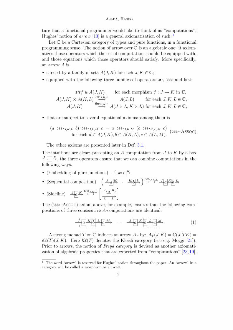
• that are subject to several equational axioms: among them is

(a >>>J,K,L b) >>>J,L,M c = a >>>J,K,M (b >>>K,L,M c)

for each a ∈ A(J,K), b ∈ A(K,L), c ∈ A(L,M).(>>>-Assoc)

The other axioms are presented later in Def. 3.1.

The intuitions are clear: presenting an A-computation from J to K by a boxJ K , the three operators ensure that we can combine computations in thefollowing ways.

• (Embedding of pure functions) Jarr f

K

• (Sequential composition)(

J a K , K b L)

>>>J,K,L7−→ J a K b L

• (Sideline) J a KfirstJ,K,L7−→

[

J a K

L L

]

The (>>>-Assoc) axiom above, for example, ensures that the following com-positions of three consecutive A-computations are identical.

J a K b L c M = J a K b L c M (1)

A strong monad T on C induces an arrow AT by: AT (J,K) = C(J, TK) =Kℓ(T )(J,K). Here Kℓ(T ) denotes the Kleisli category (see e.g. Moggi [21]).Prior to arrows, the notion of Freyd category is devised as another axiomati-zation of algebraic properties that are expected from “computations” [23,19].

1 The word “arrow” is reserved for Hughes’ notion throughout the paper. An “arrow” in acategory will be called a morphism or a 1-cell.

2

Asada, Hasuo

The latter notion of Freyd category come with a stronger categorical flavor;in Jacobs et al. [16] it is shown to be equivalent to the notion of arrow.

Remark 1.1 The previous arguments are true as long as we think of an arrowas carried by sets, with A(J,K) being a set. This is our setting. However thisis not an entirely satisfactory view in functional programming where one seesA as a type constructor—A(J,K) should rather be an object of C. In this caseone can think of several variants of arrow and Freyd category. See Atkey [2].The discussion later in the beginning of §5 is also relevant.

1.2 Arrow as Component Calculus

The current paper’s goal is to settle components as categorification of compu-tations, via (the algebraic theory of) arrows. Let us elaborate on this slogan.

A component here is in the sense of component calculi. Components aresystems which, combined with one another by some component calculus, yielda bigger, more complicated system. This “divide-and-conquer” strategy bringsorder to design processes of large-scale systems that are otherwise messed updue to the very scale and complexity of the systems to be designed.

We follow the coalgebraic modeling of components in Barbosa [5]—which isalso used in Hasuo et al. [11]—extending it later to an arrow-based modeling.In [5] a component is modeled as a coalgebra of the following type:

c : X −→(

T (X ×K))J

in Set. (2)

J c KHere J is the set of possible input to the component; K is that ofpossible output; X is the set of (internal) states of the componentwhich is a state-based machine; and T is a monad on Set that models thecomputational effect exhibited by the system. Overall, a coalgebraic compo-nent is a state-based system with specified input and output ports; it can bedrawn as above on the right.

A crucial observation here is as follows. The notion of arrow in §1.1 isto axiomatize algebraic operators on computations as boxes—such as sequen-tial composition J a K b L . Then, by regarding such boxes as componentsrather than as computations, we can employ the axiomatization of arrow asalgebraic structure on components—a component calculus—with which onecan compose components. The calculus is a basic one that allows embeddingof pure functions, sequential composition and sideline. In fact in the secondauthor’s previous work [11] with Heunen, Jacobs and Sokolova, such algebraicoperators on coalgebraic components (2) are defined and shown to satisfy theequational axioms.

3

Asada, Hasuo

1.3 Categorifying Computations into Components

Despite this similarity between computations and components, there is onelevel gap between them: from sets to categories. Let A(J,K) denote thecollection of coalgebraic components like in (2), with input-type J , output-type K and fixed effect T , but with varying state spaces X. Then it is justnatural to include morphisms between coalgebras in the overall picture, asbehavior-preserving maps (see e.g. Rutten [24]) between components. Hence

A(J,K) is now a category, specifically that of(

T ( × K))J

-coalgebras. Incontrast, with respect to computations there is no general notion of morphismbetween them, so the collection A(J,K) of A-computations is a set.

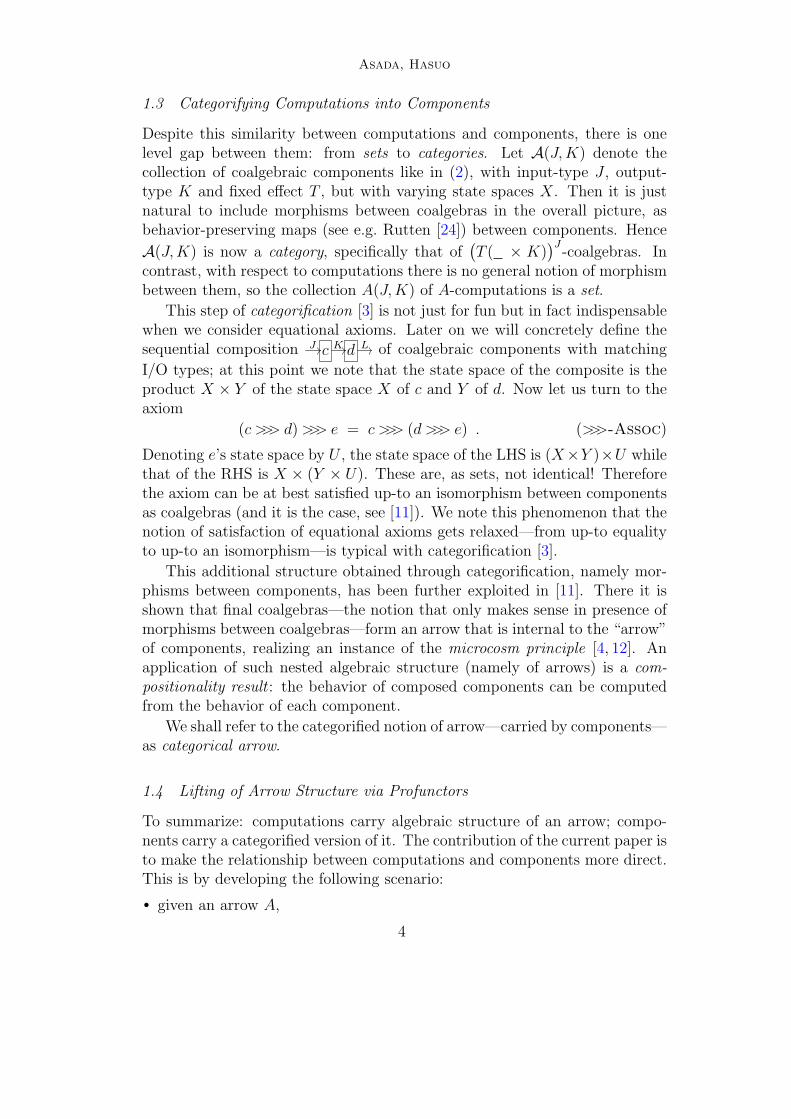
This step of categorification [3] is not just for fun but in fact indispensablewhen we consider equational axioms. Later on we will concretely define thesequential composition J c K d L of coalgebraic components with matching

I/O types; at this point we note that the state space of the composite is theproduct X × Y of the state space X of c and Y of d. Now let us turn to theaxiom

(c >>> d)>>> e = c >>> (d >>> e) . (>>>-Assoc)

Denoting e’s state space by U , the state space of the LHS is (X×Y )×U whilethat of the RHS is X × (Y × U). These are, as sets, not identical! Thereforethe axiom can be at best satisfied up-to an isomorphism between componentsas coalgebras (and it is the case, see [11]). We note this phenomenon that thenotion of satisfaction of equational axioms gets relaxed—from up-to equalityto up-to an isomorphism—is typical with categorification [3].

This additional structure obtained through categorification, namely mor-phisms between components, has been further exploited in [11]. There it isshown that final coalgebras—the notion that only makes sense in presence ofmorphisms between coalgebras—form an arrow that is internal to the “arrow”of components, realizing an instance of the microcosm principle [4, 12]. Anapplication of such nested algebraic structure (namely of arrows) is a com-positionality result : the behavior of composed components can be computedfrom the behavior of each component.

We shall refer to the categorified notion of arrow—carried by components—as categorical arrow.

1.4 Lifting of Arrow Structure via Profunctors

To summarize: computations carry algebraic structure of an arrow; compo-nents carry a categorified version of it. The contribution of the current paper isto make the relationship between computations and components more direct.This is by developing the following scenario:

• given an arrow A,

4

Asada, Hasuo

• we define the notion of (arrow-based) A-component which generalizes Bar-bosa’s modeling (2),

• and we show that these A-components carry categorical arrow structurethat is in fact a lifting of the original arrow structure of A.

Therefore: we categorify A-computations to A-components.

A weaker version of this scenario has been already presented in [11]. How-ever the last lifting part was obscured in details of direct calculations. Whatis novel in this paper is to work in Prof , the bicategory of profunctors. Infact, it is one theme of this paper to demonstrate use of calculations in Prof .

The starting point for this profunctor approach is [16]. There the arr, >>>-fragment of arrow (without first) is identified with a monoid in the category[Cop×C,Set] of bifunctors, where the latter is equipped with suitable monoidalstructure. This means—in terms of profunctors that will be described in §2—that an arrow A (without first) is a monad in Prof , in an internal sense likein Street [25].

What really made our profunctor approach feasible was a further obser-vation by the first author [1]. There the remaining first operator—whosemathematical nature was buried away in its dinaturality—is identified with acertain 2-cell in Prof . In fact, this 2-cell is a strength in an internal sense.Therefore an arrow (with its full set of operators, arr, >>> and first) is a strongmonad in Prof . This observation pleasantly parallels the informal view ofarrows as generalization of strong monads.

1.5 Organization of the Paper

In §2 we will introduce the necessary notions of dinatural transformation,(co)end and profunctor, in a rather leisurely pace. The two forms of theYoneda lemma—the end- and coend-forms—are basic there. The materialsthere are essentially extracted from Kelly [17], which is a useful reference alsoin the current non-enriched (i.e. Set-enriched) setting. In §3 we follow [1, 16]and identify an arrow with an internal strong monad in Prof , setting Prof

as our universe of discourse. In §4 we generalize Barbosa’s coalgebraic com-ponents into arrow-based components. The main result—arrow-based com-ponents form a categorical arrow—is stated there. Its actual proof is in thesubsequent §5 which is devoted to manipulation of 2-cells in Prof .

2 Categorical Preliminaries

2.1 End and Coend

In the sequel we shall often encounter a functor of the type F : Cop ×C → D,where a category C occurs twice with different variance. Given two such

5

Asada, Hasuo

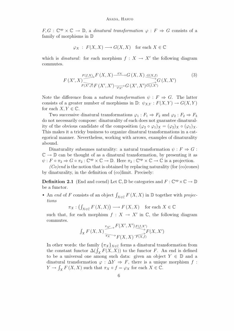
F,G : Cop × C → D, a dinatural transformation ϕ : F ⇒ G consists of afamily of morphisms in D

ϕX : F (X,X) −→ G(X,X) for each X ∈ C

which is dinatural : for each morphism f : X → X ′ the following diagramcommutes.

F (X,X)ϕX G (X,X) G(X,f)

F (X ′, X)F (f,X)

F (X′,f)

G (X,X ′)F (X ′, X ′) ϕX′

G (X ′, X ′)G(f,X′)

(3)

Note the difference from a natural transformation ψ : F ⇒ G. The latterconsists of a greater number of morphisms in D: ψX,Y : F (X,Y ) → G(X,Y )for each X,Y ∈ C.

Two successive dinatural transformations ϕ1 : F1 ⇒ F2 and ϕ2 : F2 ⇒ F3

do not necessarily compose: dinaturality of each does not guarantee dinatural-ity of the obvious candidate of the composition (ϕ2 ◦ ϕ1)X = (ϕ2)X ◦ (ϕ1)X .This makes it a tricky business to organize dinatural transformations in a cat-egorical manner. Nevertheless, working with arrows, examples of dinaturalityabound.

Dinaturality subsumes naturality: a natural transformation ψ : F ⇒ G :C → D can be thought of as a dinatural transformation, by presenting it asψ : F ◦ π2 ⇒ G ◦ π2 : Cop × C → D. Here π2 : Cop × C → C is a projection.

(Co)end is the notion that is obtained by replacing naturality (for (co)cones)by dinaturality, in the definition of (co)limit. Precisely:

Definition 2.1 (End and coend) Let C,D be categories and F : Cop×C → D

be a functor.

• An end of F consists of an object∫

X∈CF (X,X) in D together with projec-

tions

πX :(∫

X∈CF (X,X)

)

−→ F (X,X) for each X ∈ C

such that, for each morphism f : X → X ′ in C, the following diagramcommutes.

F (X ′, X ′)F (f,X′)∫

XF (X,X)

πX′

πX

F (X,X ′)F (X,X) F (X,f)

In other words: the family {πX}X∈C forms a dinatural transformation fromthe constant functor ∆(

∫

XF (X,X)) to the functor F . An end is defined

to be a universal one among such data: given an object Y ∈ D and adinatural transformation ϕ : ∆Y ⇒ F , there is a unique morphism f :Y →

∫

XF (X,X) such that πX ◦ f = ϕX for each X ∈ C.

6

Asada, Hasuo

• A coend of F is a dual notion of an end. It consists of an object∫ X∈C

F (X,X)

in D together with injections ιX : F (X,X) →∫ X

F (X,X) for each X ∈ C.Its universality, together with that of an end, can be written as follows.

f : Y −→∫

XF (X,X)

ϕX : Y → F (X,X) , dinatural in X

f :∫ X

F (X,X) −→ Y

ϕX : F (X,X) → Y, dinatural in X

(Co)ends need not exist; they do exist for example when C is small and D is(co)complete. See below.

The reader is referred to Mac Lane [20, Chap. IX] for more on (co)ends.Described there is the way to transform a functor F : Cop × C → D intoF § : C§ → D, in such a way that the (co)end of F coincides with the (co)limitof F §. Therefore existence of (co)ends depends on the (co)completeness prop-erty of D. In fact (co)end subsumes (co)limit, just as dinaturality subsumesnaturality. Therefore a useful notational convention is to denote (co)limits

also as (co)ends: for example ColimXFX as∫ X

FX.

Recalling the construction of any limit by a product and an equalizer [20,§V.2], an intuition about an end

∫

XF (X,X) is as follows: it is the product

∏

X F (X,X) which is “cut down” so as to satisfy dinaturality. Dually, a coend∫ X

F (X,X) is the coproduct∐

X F (X,X) quotiented modulo dinaturality.

2.2 Two Forms of the Yoneda Lemma

A typical example of an end arises as a set of (di)natural transformations.Given a small category C and functors F,G : Cop × C → Set, we obtain abifunctor

[F (+,−), G(−,+)] : Cop × C −→ Set , (X,Y ) 7−→ [F (Y,X), G(X,Y )] .

(4)Here [S, T ] denotes the set of functions from S to T , i.e. an exponential inSet. Note the variance: since [−,+] is contravariant in its first argument, thevariance of arguments of F is opposed in (4). Taking this functor (4) as Fin Def. 2.1, we define an end

∫

X[F (X,X), G(X,X)]. Such an end does exist

when C is a small category, because Set has small limits (hence small ends).

Proposition 2.2 Let us denote the set of dinatural transformations from F

to G by Dinat(F,G). We have a canonical isomorphism in Set:

Dinat(F,G)∼=

−→∫

X[F (X,X), G(X,X)] .

7

Asada, Hasuo

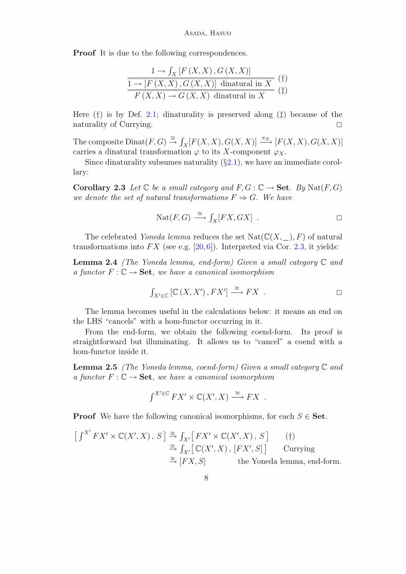
Proof It is due to the following correspondences.

1 →∫

X[F (X,X) , G (X,X)]

1 → [F (X,X) , G (X,X)] dinatural in X(†)

F (X,X) → G (X,X) dinatural in X(‡)

Here (†) is by Def. 2.1; dinaturality is preserved along (‡) because of thenaturality of Currying. 2

The composite Dinat(F,G)∼=→

∫

X[F (X,X), G(X,X)]

πX−→ [F (X,X), G(X,X)]carries a dinatural transformation ϕ to its X-component ϕX .

Since dinaturality subsumes naturality (§2.1), we have an immediate corol-lary:

Corollary 2.3 Let C be a small category and F,G : C → Set. By Nat(F,G)we denote the set of natural transformations F ⇒ G. We have

Nat(F,G)∼=

−→∫

X[FX,GX] . 2

The celebrated Yoneda lemma reduces the set Nat(C(X, ), F ) of naturaltransformations into FX (see e.g. [20,6]). Interpreted via Cor. 2.3, it yields:

Lemma 2.4 (The Yoneda lemma, end-form) Given a small category C anda functor F : C → Set, we have a canonical isomorphism

∫

X′∈C[C (X,X ′) , FX ′]

∼=−→ FX . 2

The lemma becomes useful in the calculations below: it means an end onthe LHS “cancels” with a hom-functor occurring in it.

From the end-form, we obtain the following coend-form. Its proof isstraightforward but illuminating. It allows us to “cancel” a coend with ahom-functor inside it.

Lemma 2.5 (The Yoneda lemma, coend-form) Given a small category C anda functor F : C → Set, we have a canonical isomorphism

∫ X′∈CFX ′ × C(X ′, X)

∼=−→ FX .

Proof We have the following canonical isomorphisms, for each S ∈ Set.

[ ∫ X′

FX ′ × C(X ′, X) , S] ∼=→

∫

X′

[

FX ′ × C(X ′, X) , S]

(†)∼=→

∫

X′

[

C(X ′, X) , [FX ′, S]]

Currying∼=→ [FX, S] the Yoneda lemma, end-form.

8

Asada, Hasuo

Here (†) is because the hom-functor [ , S] turns a colimit into a limit [20,§V.4], hence a coend into an end. Obviously the composite isomorphism isnatural in S; therefore we have shown that

y( ∫ X′

C(X ′, X) × FX ′) ∼=−→ y(FX) : C −→ Set , (5)

where y : Cop → [C,Set] is the (contravariant) Yoneda embedding. By theYoneda lemma the functor y is full and faithful; therefore it reflects isomor-phisms. Hence (5) proves the claim. 2

2.3 Profunctor

Definition 2.6 Let C and D be small categories. A pro-functor P from C to D is a functor P : Dop ×C → Set. Itis denoted by P : C −p→ D (see on the right).

C − p−→ D

Dop × C −→ Set

The notion of profunctor is also called distributor, bimodule or module. Formore detailed treatment of profunctors see e.g. Benabou [7] and Borceux [9].

There are principally two ways to understand profunctors. One is as “gen-eralized relations”: profunctors are to functors what relations are to functions.The differences between a profunctor P : C−p→ D and a relation R : S−p→ T areas follows.

• A relation is two-valued: for each element s ∈ S and t ∈ T , R(s, t) is eitherempty (i.e. (s, t) 6∈ R) or filled (i.e. (s, t) ∈ R). In contrast, a profunctor isvalued with arbitrary sets, that is, P (Y,X) ∈ Set.

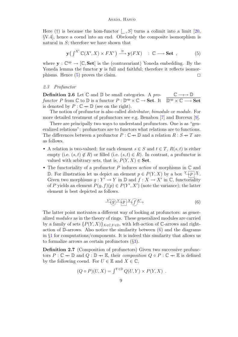
• The functoriality of a profunctor P induces action of morphisms in C and

D. For illustration let us depict an element p ∈ P (Y,X) by a box Y p X .Given two morphisms g : Y ′ → Y in D and f : X → X ′ in C, functorialityof P yields an element P (g, f)(p) ∈ P (Y ′, X ′) (note the variance); the latterelement is best depicted as follows.

Y ′g Y p X f X′

(6)

The latter point motivates a different way of looking at profunctors: as gener-alized modules as in the theory of rings. These generalized modules are carriedby a family of sets {P (Y,X)}X∈C,Y ∈D, with left-action of C-arrows and right-action of D-arrows. Also notice the similarity between (6) and the diagramsin §1 for computations/components. It is indeed this similarity that allows usto formalize arrows as certain profunctors (§3).

Definition 2.7 (Composition of profunctors) Given two successive profunc-tors P : C −p→ D and Q : D −p→ E, their composition Q ◦ P : C −p→ E is definedby the following coend. For U ∈ E and X ∈ C,

(Q ◦ P )(U,X) =∫ Y ∈D

Q(U, Y ) × P (Y,X) .

9

Asada, Hasuo

For profunctors as generalized relations, this composition operation corre-sponds to a relational composition: (S ◦ R) (x, z) if and only if ∃y.

(

R (x, y) ∧S (y, z)

)

. For profunctors as modules, it corresponds to tensor product ofmodules. In any case, recall from §2.1 that the coend in Def. 2.7 is a coprod-

uct∐

Y Q(U, Y )×P (Y,X)—a bunch of pairs ( U q Y , Y p X ), with varyingY—quotiented modulo a certain equivalence ≃. This equivalence ≃ (dictatedby dinaturality) intuitively says: the choice of intermediate Y ∈ D does notmatter. Specifically, the equivalence ≃ is generated by the following relation;here f : Y → Y ′ is a morphism in D.

(

U q Y f Y ′

, Y ′p X

)

≃(

U q Y , Y f Y ′p X

)

.

C

P

Q

ψ D

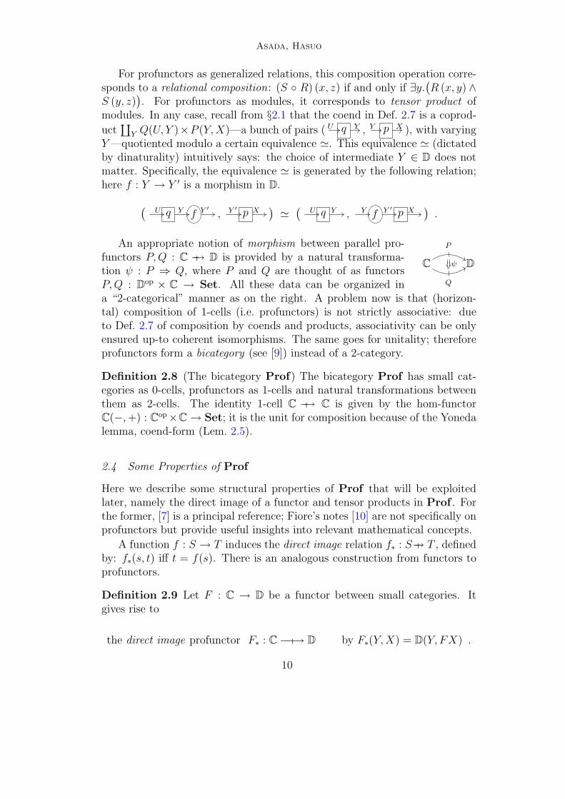
An appropriate notion of morphism between parallel pro-functors P,Q : C −p→ D is provided by a natural transforma-tion ψ : P ⇒ Q, where P and Q are thought of as functorsP,Q : Dop × C → Set. All these data can be organized ina “2-categorical” manner as on the right. A problem now is that (horizon-tal) composition of 1-cells (i.e. profunctors) is not strictly associative: dueto Def. 2.7 of composition by coends and products, associativity can be onlyensured up-to coherent isomorphisms. The same goes for unitality; thereforeprofunctors form a bicategory (see [9]) instead of a 2-category.

Definition 2.8 (The bicategory Prof) The bicategory Prof has small cat-egories as 0-cells, profunctors as 1-cells and natural transformations betweenthem as 2-cells. The identity 1-cell C −p→ C is given by the hom-functorC(−,+) : Cop×C → Set; it is the unit for composition because of the Yonedalemma, coend-form (Lem. 2.5).

2.4 Some Properties of Prof

Here we describe some structural properties of Prof that will be exploitedlater, namely the direct image of a functor and tensor products in Prof . Forthe former, [7] is a principal reference; Fiore’s notes [10] are not specifically onprofunctors but provide useful insights into relevant mathematical concepts.

A function f : S → T induces the direct image relation f∗ : S−p→ T , definedby: f∗(s, t) iff t = f(s). There is an analogous construction from functors toprofunctors.

Definition 2.9 Let F : C → D be a functor between small categories. Itgives rise to

the direct image profunctor F∗ : C − p−→ D by F∗(Y,X) = D(Y, FX) .

10

Asada, Hasuo

The mapping ( )∗ also applies to natural transformations in an obviousway; this determines a pseudo functor (see e.g. [9]) ( )∗ : Cat → Prof thatembeds Cat in Prof .

Notations 2.10 Throughout the rest of the paper, the direct image F∗ of afunctor F shall be simply denoted by F . The identity profunctor id : C−p→ C—that is the hom-functor—will be often denoted by C : C −p→ C.

The Cartesian product operator × in Cat lifts Prof ; given profunctorsF : C −p→ C

′ and G : D −p→ D′, we define

F ×G : C×D−p→ C′×D

′ by (F ×G)(X ′, Y ′, X, Y ) = F (X ′, X)×G(Y ′, Y ) .(7)

The symbol × occurring in the last denotes the Cartesian product in Set.The lifted operator × in Prof makes it a “monoidal bicategory,” a notionwhose precise definition involves delicate handling of coherence. We shall notdo that in this paper. Nevertheless, we will need the following property.

Lemma 2.11 The operation × on Prof is bifunctorial: that is, given four

profunctors CP

−p→ DQ

−p→ E and C′P ′

−p→ D′Q′

−p→ E′ we have (Q ◦ P ) × (Q′ ◦ P ′)∼=→

(Q×Q′) ◦ (P × P ′).

Proof This is due to the Fubini theorem for coends. See [20, §IX.8] 2

It is obvious that the operator × acts also on 2-cells (that are naturaltransformations).

3 Arrows as Profunctors

We review the results in [16, 1] that identify Hughes’ notion of arrow with aprofunctor with additional algebraic structure.

First we present the precise definition of arrow. Usually it is defined overa Cartesian category C. However, since it is rather the monoidal structure ofC that is essential, we shall work with a monoidal category.

Definition 3.1 (Arrow [13]) Given a monoidal category C = (C,⊗, I), anarrow over C consists of carrier sets {A(J,K)}J,K∈C and operators arr, >>> andfirst as described in §1.1. The operators must satisfy the following equational

11

Asada, Hasuo

axioms.

(a >>> b) >>> c = a >>> (b >>> c) (>>>-Assoc)

arr (g ◦ f) = arr f >>> arr g (arr-Func1)

arr idJ >>>J,J,K a = a = a >>>J,K,K arr idK (arr-Func2)

firstJ,K,I a >>> arr ρK = arr ρK >>> a (ρ-Nat)

firstJ,K,L a >>> arr(idK ⊗ f) = arr(idJ ⊗ f) >>> firstJ,K,M a (arr-Centr)

(firstJ,K,L⊗M a) >>> (arr αK,L,M ) = (arr αJ,L,M ) >>> first(first a) (α-Nat)

firstJ,K,L(arr f) = arr(f ⊗ idL) (arr-Premon)

firstJ,L,M (a >>> b) = (firstJ,K,M a) >>> (firstK,L,M b) (first-Func)

Here some subscripts are suppressed. The morphism ρK : K ⊗ I∼=→ K is the

right unitor isomorphism; α denotes an associator isomorphism. The names ofthe axioms hint their correspondence to the (premonoidal) structure of Freydcategories [23, 19].

Next we introduce the corresponding construct in Prof , which we shalltentatively call a Prof-arrow.

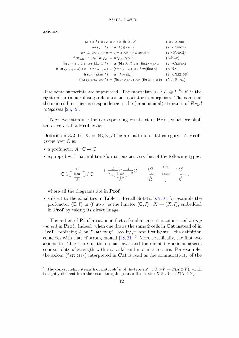
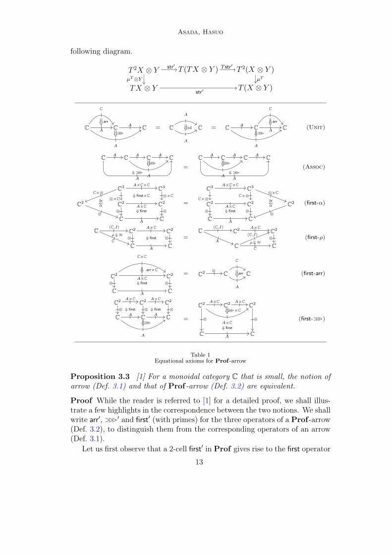
Definition 3.2 Let C = (C,⊗, I) be a small monoidal category. A Prof-arrow over C is:

• a profunctor A : C −p→ C,

• equipped with natural transformations arr, >>>, first of the following types:

C

C

A

⇓ arr C ,C

A

A

⇓>>>C

AC

,C2 A×C

⊗ ⇓ first

C2

⊗

C A C

,

where all the diagrams are in Prof ,

• subject to the equalities in Table 1. Recall Notations 2.10; for example theprofunctor 〈C, I〉 in (first-ρ) is the functor 〈C, I〉 : X 7→ (X, I), embeddedin Prof by taking its direct image.

The notion of Prof -arrow is in fact a familiar one: it is an internal strongmonad in Prof . Indeed, when one draws the same 2-cells in Cat instead of inProf—replacing A by T , arr by ηT , >>> by µT and first by str

′—the definitioncoincides with that of strong monad [18,21]. 2 More specifically, the first twoaxioms in Table 1 are for the monad laws; and the remaining axioms assertscompatibility of strength with monoidal and monad structure. For example,the axiom (first->>>) interpreted in Cat is read as the commutativity of the

2 The corresponding strength operator str′ is of the type str

′ : TX ⊗Y → T (X ⊗Y ), whichis slightly different from the usual strength operator that is str : X ⊗ TY → T (X ⊗ Y ).

12

Asada, Hasuo

following diagram.

T 2X ⊗ Ystr′

µT⊗Y

T (TX ⊗ Y ) T str′ T 2(X ⊗ Y )µT

TX ⊗ Ystr′

T (X ⊗ Y )

C

C

arr

A

A

>>>

CA

C = C

A

A

id C = CA

A

>>>

C

C

arr

AC (Unit)

CA

A

⇓ >>>

CA

A

>>>

CA

C

=

CA

A

⇓ >>>A

>>>

CA

CA

C

(Assoc)

C3 A×C×C

⊗×C

C×⊗⇓ first×C

C3

⊗×C

C2

⊗

⇐∼=α C

2

⊗A×C

⇓ first

C2

⊗

CA

C

=

C3 A×C×C

C×⊗

C3

C×⊗⊗×C

C2

⊗A×C

⇓ first

C2

⊗

⇐∼=α C

2

⊗

CA

C

(first-α)

C〈C,I〉

C

ρ ⇓∼=C

2 A×C

⊗ ⇓ first

C2

⊗

CA

C

=C

〈C,I〉

A

C2 A×C

C2

⊗

CC

ρ ⇓∼=

〈C,I〉

C

(first-ρ)

C2

C×C

arr×C

A×C

⊗ ⇓ first

C2

⊗

CA

C

= C2 ⊗

C

C

A

arr C (first-arr)

C2 A×C

⇓ first⊗

C2 A×C

⇓ first⊗

C2

⊗

CA

A

>>>

CA

C =

C2 A×C

A×C

>>>×C

⊗

C2 A×C

C2

⊗

CA

⇓ first

C

(first->>>)

Table 1Equational axioms for Prof -arrow

Proposition 3.3 [1] For a monoidal category C that is small, the notion ofarrow (Def. 3.1) and that of Prof-arrow (Def. 3.2) are equivalent.

Proof While the reader is referred to [1] for a detailed proof, we shall illus-trate a few highlights in the correspondence between the two notions. We shallwrite arr

′, >>>′ and first′ (with primes) for the three operators of a Prof -arrow

(Def. 3.2), to distinguish them from the corresponding operators of an arrow(Def. 3.1).

Let us first observe that a 2-cell first′ in Prof gives rise to the first operator

13

Asada, Hasuo

in Def. 3.1. The former is an element of the LHS below, where >>> denotescomposition of profunctors (Def. 2.7).

Nat(

(⊗ ◦ (A× C))(−,+1,+2) , (A ◦ ⊗)(−,+1,+2))

∼=∫

X,K,Y ∈C

[

(⊗ ◦ (A× C))(X,K, Y ) , (A ◦ ⊗)(X,K, Y )]

by Cor. 2.3

∼=∫

X,K,Y

[ ∫ J,LC(X, J ⊗ L) × A(J,K) × C(L, Y ) ,

∫ UA(X,U) × C(U,K ⊗ Y )

]

by Def. 2.7, Def. 2.9 and (7)

∼=∫

X,K,Y,J,L

[

C(X, J ⊗ L) × A(J,K) × C(L, Y ) ,∫ U

A(X,U) × C(U,K ⊗ Y )]

since a hom-functor [−, S] turns a coend into an end∼=

∫

X,K,Y,J,L

[

C(X, J ⊗ L),[

A(J,K),[

C(L, Y ) ,∫ U

A(X,U) × C(U,K ⊗ Y )]]]

by Currying∼=

∫

J,K,L

[

A(J,K), A(J ⊗ L,K ⊗ L)]

by canceling X,Y by Lem. 2.4 and U by Lem. 2.5∼= NatJ,KDinatL

(

A(J,K), A(J ⊗ L,K ⊗ L))

by Prop. 2.2 and Cor. 2.3.

Therefore a 2-cell first′ in Prof gives rise to a family of functions A(J,K) →

A(J ⊗ L,K ⊗ L) that is natural in J,K and dinatural in L. This is preciselythe type of the first operator in Def. 3.1. The equational axioms of an arroware indeed satisfied due to those of a Prof -arrow. We note that the axiom(arr-Centr) is satisfied not because of any specific axiom of a Prof -arrow,but because of the dinaturality of first

′ as a 2-cell in Prof .

For the reverse direction where an arrow induces a Prof -arrow, we haveto equip the carrier {A(J,K)}J,K of an arrow with action of morphisms in C,rendering A into a functor Cop × C → Set. This is done with the help ofarrow operators. Specifically, A(g, f)(a) := arrf >>> a >>> arrg, that is:

Y ′

fY a X g X′

:= Y ′

arrfY a X arrg X′

.

Each of the arrow operators yield its corresponding Prof -arrow operator; thelatter’s (di)naturality is derived from the arrow axioms. So are the equationalaxioms for a Prof -arrow. 2

Prop. 3.3 offers a novel mathematical understanding of the notion of arrow.Its axiomatization seems to have stronger justifications than the original one(Def. 3.1) does. It also seems simpler than the treatment of first in Freydcategories which involves technicalities like premonoidal categories and centralmorphisms. It is this simplicity that is exploited in the rest of the paper.

When the base monoidal category C is symmetric—which is our setting inthe sequel—we can obtain another sideline operator second.

Definition 3.4 Let A be an arrow over a small symmetric monoidal category

14

Asada, Hasuo

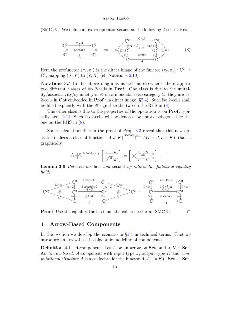
(SMC) C. We define an extra operator second as the following 2-cell in Prof .

C2 C×A

⊗ ⇓ second

C2

⊗

C A C

:=

C2 C×A

〈π2,π1〉

⊗ ∼=⇐

C2

〈π2,π1〉

⊗∼=⇐C2 A×C

⊗ ⇓ first

C2

⊗

C A C

(8)

Here the profunctor 〈π2, π1〉 is the direct image of the functor 〈π2, π1〉 : C2 →C2, mapping (X,Y ) to (Y,X) (cf. Notations 2.10).

Notations 3.5 In the above diagrams as well as elsewhere, there appeartwo different classes of iso 2-cells in Prof . One class is due to the unital-ity/associativity/symmetry of ⊗ on a monoidal base category C; they are iso2-cells in Cat embedded in Prof via direct image (§2.4). Such iso 2-cells shallbe filled explicitly with the ∼= sign, like the two on the RHS in (8).

The other class is due to the properties of the operation × on Prof , typi-cally Lem. 2.11. Such iso 2-cells will be denoted by empty polygons, like theone on the RHS in (8).

Some calculations like in the proof of Prop. 3.3 reveal that this new op-

erator realizes a class of functions A(J,K)secondJ,K,L

−→ A(L× J, L×K), that isgraphically

J a KsecondJ,K,L

7−→

[

L L

JaK

]

:=

[

J a K

L L

]

.

Lemma 3.6 Between the first and second operators, the following equalityholds.

C3 C×A×C

⊗×CC×⊗

⇓ second×C

C3

⊗×CC×⊗

C2

⊗

∼=⇐ C2 A×C

⊗ ⇓ first

C2

⊗

∼=⇐ C2⊗

C A C

=

C3 C×A×C

C×⊗ ⇓C×first

C3

C×⊗

C2 C×A

⊗ ⇓ second

C2

⊗

C A C

Proof Use the equality (first-α) and the coherence for an SMC C. 2

4 Arrow-Based Components

In this section we develop the scenario in §1.4 in technical terms. First weintroduce an arrow-based coalgebraic modeling of components.

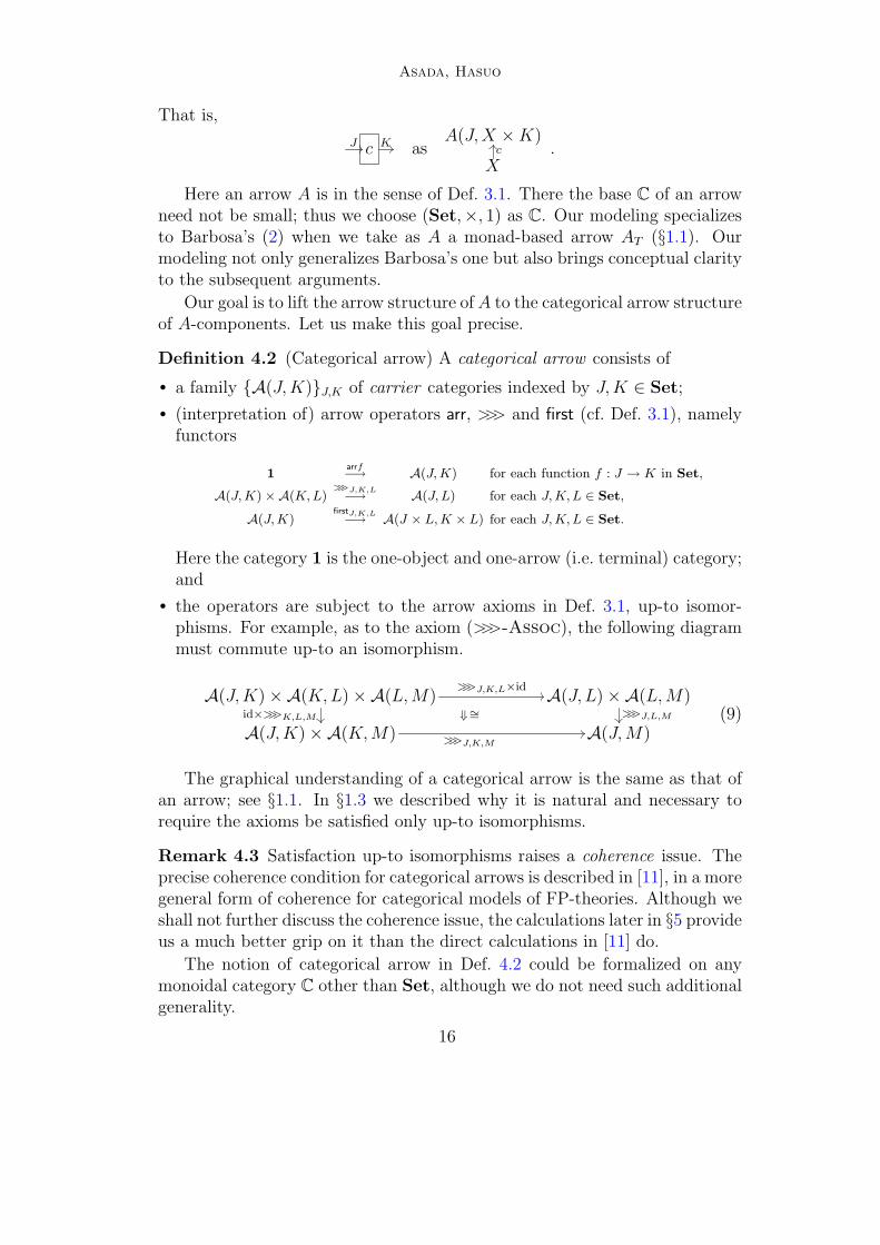
Definition 4.1 (A-component) Let A be an arrow on Set, and J,K ∈ Set.An (arrow-based) A-component with input-type J , output-type K and com-putational structure A is a coalgebra for the functor A(J, ×K) : Set → Set.

15

Asada, Hasuo

That is,

J c K asA(J,X ×K)

Xc .

Here an arrow A is in the sense of Def. 3.1. There the base C of an arrowneed not be small; thus we choose (Set,×, 1) as C. Our modeling specializesto Barbosa’s (2) when we take as A a monad-based arrow AT (§1.1). Ourmodeling not only generalizes Barbosa’s one but also brings conceptual clarityto the subsequent arguments.

Our goal is to lift the arrow structure ofA to the categorical arrow structureof A-components. Let us make this goal precise.

Definition 4.2 (Categorical arrow) A categorical arrow consists of

• a family {A(J,K)}J,K of carrier categories indexed by J,K ∈ Set;

• (interpretation of) arrow operators arr, >>> and first (cf. Def. 3.1), namelyfunctors

1arrf−→ A(J, K) for each function f : J → K in Set,

A(J, K) ×A(K, L)>>>J,K,L−→ A(J, L) for each J, K, L ∈ Set,

A(J, K)firstJ,K,L−→ A(J × L, K × L) for each J, K, L ∈ Set.

Here the category 1 is the one-object and one-arrow (i.e. terminal) category;and

• the operators are subject to the arrow axioms in Def. 3.1, up-to isomor-phisms. For example, as to the axiom (>>>-Assoc), the following diagrammust commute up-to an isomorphism.

A(J,K) ×A(K,L) ×A(L,M)>>>J,K,L×id

id×>>>K,L,M ⇓∼=

A(J, L) ×A(L,M)>>>J,L,M

A(J,K) ×A(K,M) >>>J,K,MA(J,M)

(9)

The graphical understanding of a categorical arrow is the same as that ofan arrow; see §1.1. In §1.3 we described why it is natural and necessary torequire the axioms be satisfied only up-to isomorphisms.

Remark 4.3 Satisfaction up-to isomorphisms raises a coherence issue. Theprecise coherence condition for categorical arrows is described in [11], in a moregeneral form of coherence for categorical models of FP-theories. Although weshall not further discuss the coherence issue, the calculations later in §5 provideus a much better grip on it than the direct calculations in [11] do.

The notion of categorical arrow in Def. 4.2 could be formalized on anymonoidal category C other than Set, although we do not need such additionalgenerality.

16

Asada, Hasuo

The main contribution of this paper is the following result as well as itsproof presented using the rest of the paper.

Theorem 4.4 (Main contribution) Let A be an arrow on Set. The categories{Coalg(A(J, ×K) )}J,K of A-components carry a categorical arrow.

On top of it, we can appeal to the formalization [12, 11] of the microcosmprinciple [4] to obtain the following compositionality result.

Corollary 4.5 In the setting of Thm. 4.4, assume further that for each J,K ∈Set the functor A(J, ×K) has a final coalgebra ζJ,K : ZJ,K

∼=→ A(J, ZJ,K×K).

(i) The family {ZJ,K}J,K is canonically an arrow.

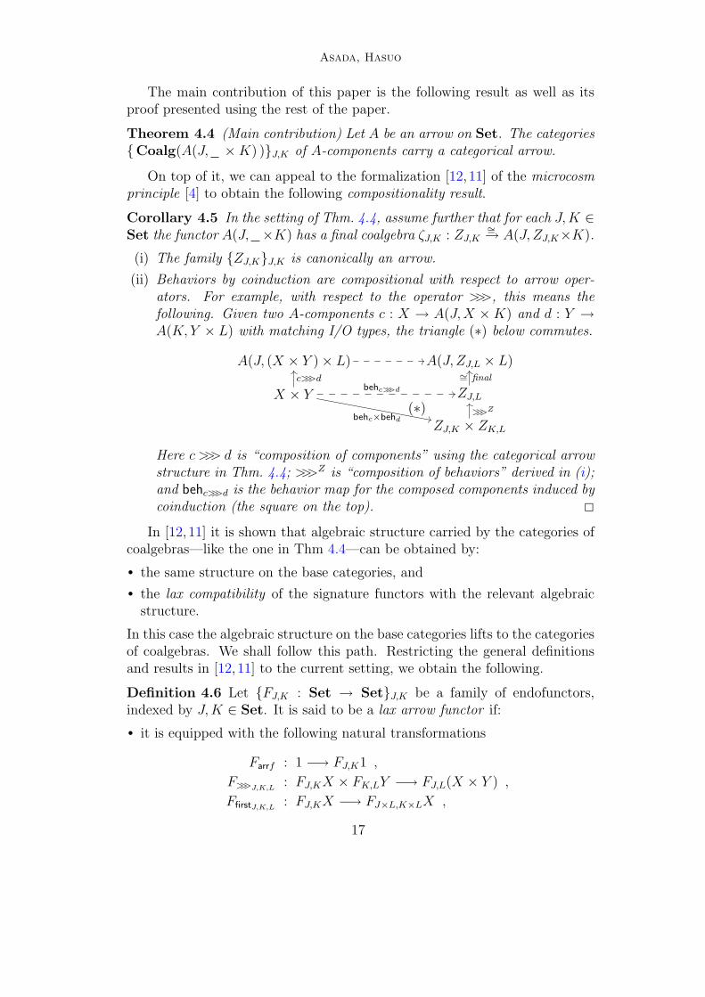
(ii) Behaviors by coinduction are compositional with respect to arrow oper-ators. For example, with respect to the operator >>>, this means thefollowing. Given two A-components c : X → A(J,X ×K) and d : Y →A(K,Y × L) with matching I/O types, the triangle (∗) below commutes.

A(J, (X × Y ) × L) A(J, ZJ,L × L)

X × Y

c>>>dbehc>>>d

(∗)behc×behd

ZJ,L

∼= final

ZJ,K × ZK,L

>>>Z

Here c >>> d is “composition of components” using the categorical arrowstructure in Thm. 4.4; >>>Z is “composition of behaviors” derived in (i);and behc>>>d is the behavior map for the composed components induced bycoinduction (the square on the top). 2

In [12, 11] it is shown that algebraic structure carried by the categories ofcoalgebras—like the one in Thm 4.4—can be obtained by:

• the same structure on the base categories, and

• the lax compatibility of the signature functors with the relevant algebraicstructure.

In this case the algebraic structure on the base categories lifts to the categoriesof coalgebras. We shall follow this path. Restricting the general definitionsand results in [12,11] to the current setting, we obtain the following.

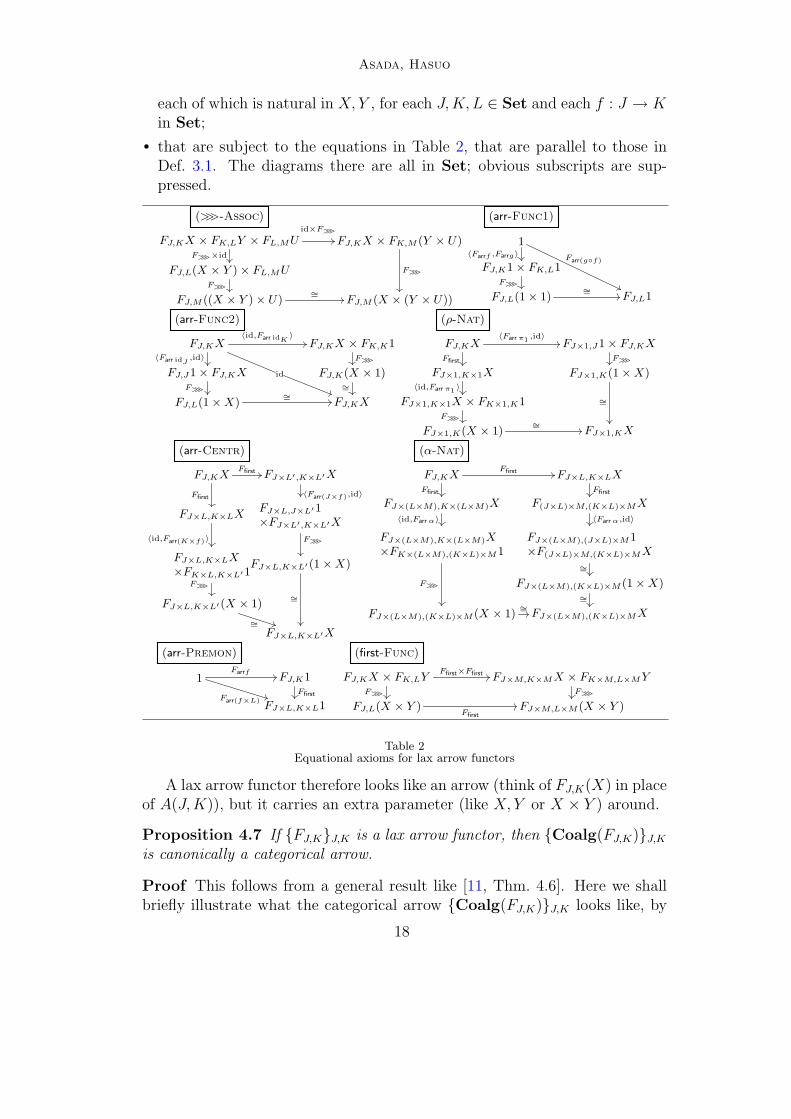
Definition 4.6 Let {FJ,K : Set → Set}J,K be a family of endofunctors,indexed by J,K ∈ Set. It is said to be a lax arrow functor if:

• it is equipped with the following natural transformations

Farrf : 1 −→ FJ,K1 ,

F>>>J,K,L: FJ,KX × FK,LY −→ FJ,L(X × Y ) ,

FfirstJ,K,L: FJ,KX −→ FJ×L,K×LX ,

17

Asada, Hasuo

each of which is natural in X,Y , for each J,K,L ∈ Set and each f : J → K

in Set;

• that are subject to the equations in Table 2, that are parallel to those inDef. 3.1. The diagrams there are all in Set; obvious subscripts are sup-pressed.

FJ,KX × FK,LY × FL,MU

(>>>-Assoc)id×F>>>

F>>>×id

FJ,KX × FK,M (Y × U)

F>>>FJ,L(X × Y ) × FL,MUF>>>

FJ,M ((X × Y ) × U)∼=

FJ,M (X × (Y × U))

1

(arr-Func1)

Farr(g◦f)〈Farrf ,Farrg〉

FJ,K1 × FK,L1F>>>

FJ,L(1 × 1)∼= FJ,L1

FJ,KX

(arr-Func2)〈id,Farr idK

〉

〈Farr idJ,id〉

id

FJ,KX × FK,K1F>>>

FJ,J1 × FJ,KXF>>>

FJ,K(X × 1)∼=

FJ,L(1 × X)∼= FJ,KX

FJ,KX

(ρ-Nat)

〈Farr π1,id〉

Ffirst

FJ×1,J1 × FJ,KXF>>>

FJ×1,K×1X〈id,Farr π1

〉

FJ×1,K(1 × X)

∼=FJ×1,K×1X × FK×1,K1F>>>

FJ×1,K(X × 1)∼= FJ×1,KX

FJ,KX

(arr-Centr)

Ffirst

Ffirst

FJ×L′,K×L′X

〈Farr(J×f),id〉

FJ×L,K×LX

〈id,Farr(K×f)〉

FJ×L,J×L′1×FJ×L′,K×L′X

F>>>

FJ×L,K×LX

×FK×L,K×L′1F>>>

FJ×L,K×L′(1 × X)

∼=FJ×L,K×L′(X × 1)

∼=FJ×L,K×L′X

FJ,KX

(α-Nat)

Ffirst

Ffirst

FJ×L,K×LXFfirst

FJ×(L×M),K×(L×M)X

〈id,Farr α〉

F(J×L)×M,(K×L)×MX

〈Farr α,id〉

FJ×(L×M),K×(L×M)X

×FK×(L×M),(K×L)×M1

F>>>

FJ×(L×M),(J×L)×M1×F(J×L)×M,(K×L)×MX

∼=

FJ×(L×M),(K×L)×M (1 × X)∼=

FJ×(L×M),(K×L)×M (X × 1)∼= FJ×(L×M),(K×L)×MX

1

(arr-Premon)

Farrf

Farr(f×L)

FJ,K1Ffirst

FJ×L,K×L1

FJ,KX × FK,LY

(first-Func)

Ffirst×Ffirst

F>>>

FJ×M,K×MX × FK×M,L×MYF>>>

FJ,L(X × Y )Ffirst

FJ×M,L×M (X × Y )

Table 2Equational axioms for lax arrow functors

A lax arrow functor therefore looks like an arrow (think of FJ,K(X) in placeof A(J,K)), but it carries an extra parameter (like X,Y or X × Y ) around.

Proposition 4.7 If {FJ,K}J,K is a lax arrow functor, then {Coalg(FJ,K)}J,Kis canonically a categorical arrow.

Proof This follows from a general result like [11, Thm. 4.6]. Here we shallbriefly illustrate what the categorical arrow {Coalg(FJ,K)}J,K looks like, by

18

Asada, Hasuo

describing the sequential composition >>> : Coalg(FJ,K) × Coalg(FK,L) −→Coalg(FJ,L). Using F>>> in Def. 4.6 it is defined as follows.

(

FJ,KX

X

c ,FK,LY

Y

d

)

>>>7−→

FJ,L(X × Y )

FJ,KX × FK,LYF>>>

X × Yc×d

The definitions are similar for the other arrow operators. The arrow axiomsare satisfied due to the corresponding equational condition on the lax arrowfunctor. 2

This proposition reduces our goal (Thm. 4.4) to showing that the family{A(J, × K)}J,K is a lax arrow functor. This is what will be shown in thenext section, through manipulation of 2-cells in Prof .

5 Calculations in Prof

There is one technical issue in front of us: the size issue. The 0-cells of Prof

are small categories; the smallness restriction is necessary for composition ofprofunctors to be well-defined (Def. 2.7). However, with Set being not small,the arrow A in Def. 4.1 cannot be a 1-cell in Prof . The arrow A needs to bebased on Set so that A(J, ×K) is an endofunctor Set → Set.

In this paper we shall get round of the problem by pretending that Set issmall. There are two possible justifications.

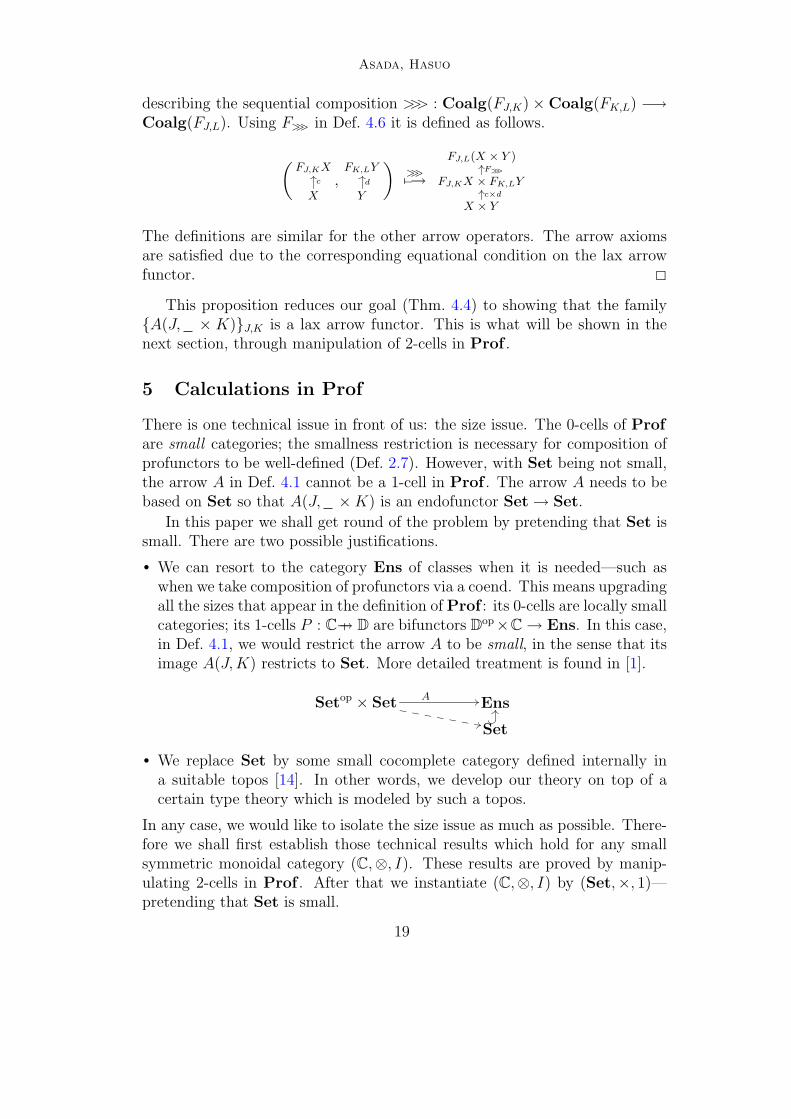
• We can resort to the category Ens of classes when it is needed—such aswhen we take composition of profunctors via a coend. This means upgradingall the sizes that appear in the definition of Prof : its 0-cells are locally smallcategories; its 1-cells P : C−p→ D are bifunctors Dop×C → Ens. In this case,in Def. 4.1, we would restrict the arrow A to be small, in the sense that itsimage A(J,K) restricts to Set. More detailed treatment is found in [1].

Setop × SetA

Ens

Set

• We replace Set by some small cocomplete category defined internally ina suitable topos [14]. In other words, we develop our theory on top of acertain type theory which is modeled by such a topos.

In any case, we would like to isolate the size issue as much as possible. There-fore we shall first establish those technical results which hold for any smallsymmetric monoidal category (C,⊗, I). These results are proved by manip-ulating 2-cells in Prof . After that we instantiate (C,⊗, I) by (Set,×, 1)—pretending that Set is small.

19

Asada, Hasuo

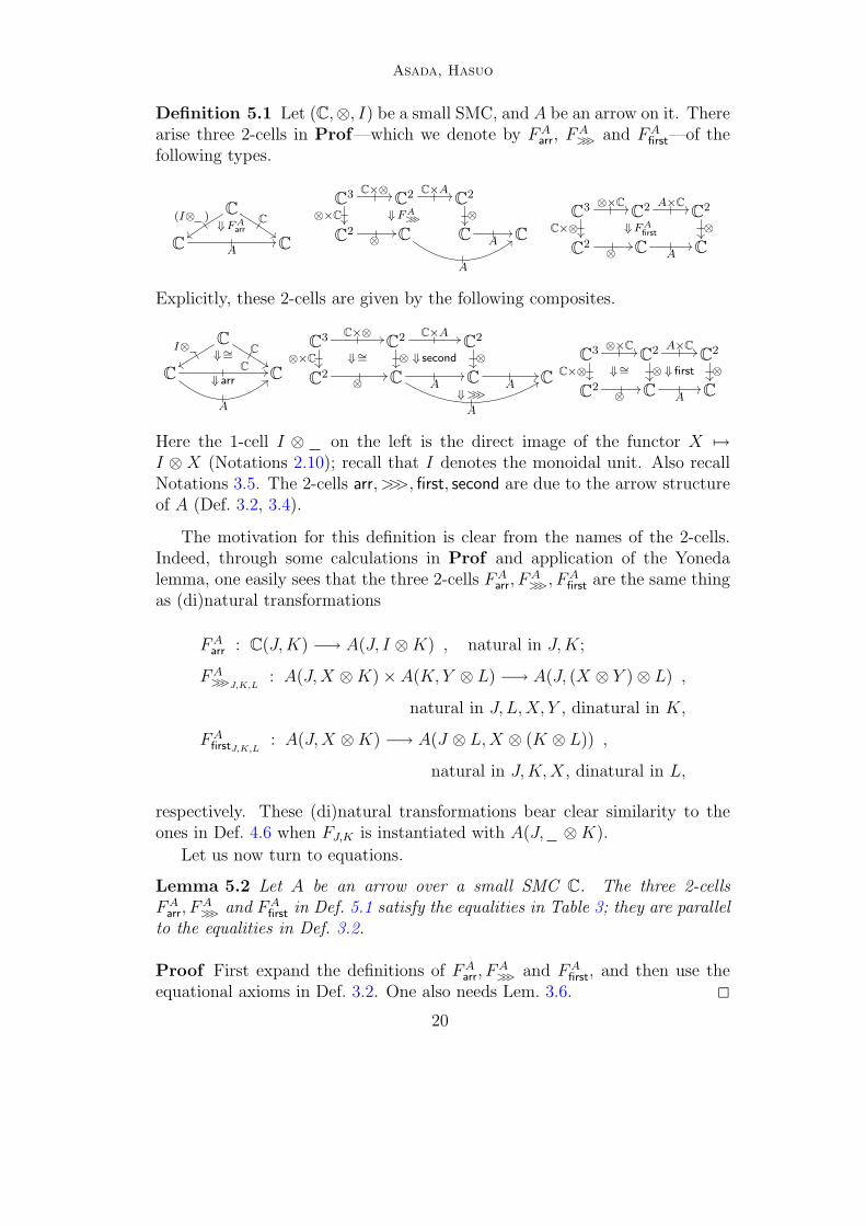
Definition 5.1 Let (C,⊗, I) be a small SMC, and A be an arrow on it. Therearise three 2-cells in Prof—which we denote by FA

arr, FA

>>> and FAfirst

—of thefollowing types.

CC(I⊗ )

C A

⇓FAarr

C

C3 C×⊗

⊗×C

C2 C×A

⇓FA>>>

C2

⊗

C2⊗ C

A

C A C

C3 ⊗×C

C×⊗

C2 A×C

⇓FAfirst

C2

⊗

C2⊗ C A C

Explicitly, these 2-cells are given by the following composites.

CCI⊗

CC

⇓ arr

A

⇓∼=

C

C3 C×⊗

⊗×C ⇓∼=

C2 C×A

⊗ ⇓ second

C2

⊗

C2⊗ C A

A

⇓>>>

C A C

C3 ⊗×C

C×⊗ ⇓∼=

C2 A×C

⊗ ⇓ first

C2

⊗

C2⊗ C A C

Here the 1-cell I ⊗ on the left is the direct image of the functor X 7→I ⊗X (Notations 2.10); recall that I denotes the monoidal unit. Also recallNotations 3.5. The 2-cells arr, >>>, first, second are due to the arrow structureof A (Def. 3.2, 3.4).

The motivation for this definition is clear from the names of the 2-cells.Indeed, through some calculations in Prof and application of the Yonedalemma, one easily sees that the three 2-cells FA

arr, FA

>>>, FAfirst

are the same thingas (di)natural transformations

FAarr

: C(J,K) −→ A(J, I ⊗K) , natural in J,K;

FA>>>J,K,L

: A(J,X ⊗K) × A(K,Y ⊗ L) −→ A(J, (X ⊗ Y ) ⊗ L) ,

natural in J, L,X, Y , dinatural in K,

FAfirstJ,K,L

: A(J,X ⊗K) −→ A(J ⊗ L,X ⊗ (K ⊗ L)) ,

natural in J,K,X, dinatural in L,

respectively. These (di)natural transformations bear clear similarity to theones in Def. 4.6 when FJ,K is instantiated with A(J, ⊗K).

Let us now turn to equations.

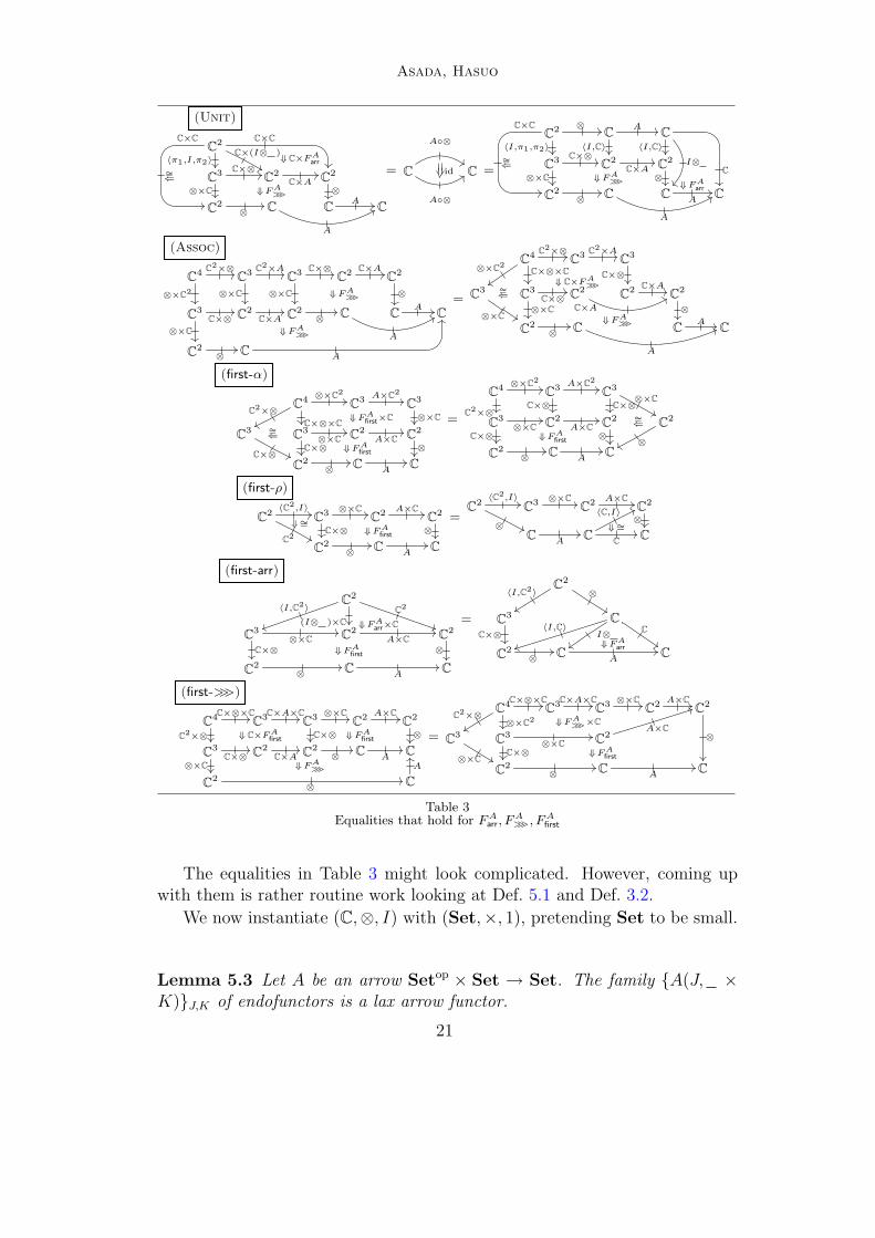
Lemma 5.2 Let A be an arrow over a small SMC C. The three 2-cellsFA

arr, FA

>>> and FAfirst

in Def. 5.1 satisfy the equalities in Table 3; they are parallelto the equalities in Def. 3.2.

Proof First expand the definitions of FAarr, FA

>>> and FAfirst

, and then use theequational axioms in Def. 3.2. One also needs Lem. 3.6. 2

20

Asada, Hasuo

C2

(Unit)

〈π1,I,π2〉C×(I⊗ )

C×CC×C

∼=⇐ C

3 C×⊗

⊗×C

C2

C×A

⇓ C×F Aarr

⇓ F A>>>

C2

⊗

C2

⊗ C

A

CA

C

= C

A◦⊗

A◦⊗

id C =

C2

〈I,π1,π2〉

⊗C×C

∼=⇐

C

〈I,C〉

AC

〈I,C〉

I⊗C

C3 C×⊗

⊗×C

C2

C×A⇓ F A

>>>

C2

⊗

C2

⊗ C

A

CA

⇓ F Aarr

C

C4

(Assoc)

C2×⊗

⊗×C2

C3 C

2×A

⊗×C

C3 C×⊗

⊗×C

C2 C×A

C2

⊗

C3

⊗×C

C×⊗ C2

C×A C2

⊗

⇓ F A>>>

C

A

⇓ F A>>>

CA

C

C2

⊗ CA

=

C4 C

2×⊗

C×⊗×C⊗×C2

C3 C

2×AC

3

C×⊗

C3

⊗×C

∼=⇐ C

3C×⊗

⊗×C

C2

C×A

⇓ F A>>>

⇓ C×F A>>>

C2 C×A

C2

⊗

C2

⊗ C

A

CA

C

(first-α)

C4 ⊗×C

2

C×⊗×C

C2×⊗

⇓ F Afirst

×C

C3 A×C

2

C3

⊗×C

C3

C×⊗

∼=⇐ C

3

C×⊗⊗×C

⇓ F Afirst

C2

A×CC

2

⊗

C2

⊗ CA

C

=

C4 ⊗×C

2

C2×⊗

C3 A×C

2

C×⊗

C3

C×⊗⊗×C

C3

⊗×C

C×⊗ ⇓ F Afirst

C2

A×CC

2

⊗

∼=⇐ C

2

⊗

C2

⊗ CA

C

C2

(first-ρ)

〈C2,I〉

C2

⇓∼=C

3 ⊗×C

C×⊗ ⇓ F Afirst

C2 A×C

C2

⊗

C2

⊗ CA

C

=C

2〈C

2,I〉

⊗

C3 ⊗×C

C2 A×C

C2

⊗

CA

C

〈C,I〉

C

⇓∼=C

(first-arr)

C2

〈I,C2〉

(I⊗ )×C

C2

C3

⊗×C

C×⊗ ⇓ F Afirst

C2

A×C

⇓ F Aarr

×C

C2

⊗

C2

⊗ CA

C

=

C2

〈I,C2〉 ⊗

C3

C×⊗

C〈I,C〉

I⊗C

C2

⊗ CA

⇓ F Aarr

C

C4

(first->>>)

C×⊗×C

⇓ C×F AfirstC

2×⊗

C3C×A×C

C3 ⊗×C

⇓ F Afirst

C×⊗

C2 A×C

C2

⊗

C3

C×⊗⊗×C

C2

C×A C2

⊗⇓ F A

>>>

CA

C

C2

⊗ C

A

=

C4C×⊗×C

⇓ F A>>>×C⊗×C

2C2×⊗

C3C×A×C

C3 ⊗×C

C2 A×C

C2

⊗C3

⊗×C

C3

⊗×C

C×⊗

C2

A×C

⇓ F Afirst

C2

⊗ CA

C

Table 3Equalities that hold for F A

arr, FA>>>, F A

first

The equalities in Table 3 might look complicated. However, coming upwith them is rather routine work looking at Def. 5.1 and Def. 3.2.

We now instantiate (C,⊗, I) with (Set,×, 1), pretending Set to be small.

Lemma 5.3 Let A be an arrow Setop × Set → Set. The family {A(J, ×K)}J,K of endofunctors is a lax arrow functor.

21

Asada, Hasuo

Proof The three 2-cells in Def. 5.1 provide the three natural transformationsrequired in Def. 4.6. The equations asserted in Def. 4.6 follow from those inLem. 5.2. Checking all this is (laborious) routine work. 2

Combining Prop. 4.7 and Lem. 5.3, our main result Thm. 4.4 is proved.

Remark 5.4 A characterization of categorical arrows in the spirit of Prop. 3.3can possibly yield a even more direct proof of Thm. 4.4. Unfortunately untilnow we lack necessary infrastructure such as a lifting result like Prop. 4.7. Weare currently investigating possible formalization using fibered spans (see e.g.Jacobs [15]).

In Prof the trace operator for an arrow (loop in Paterson [22], see alsoBenton and Hyland [8]) can be formalized in a similar way to other operatorslike >>>. Its description as well as possible application to components willpresented in another venue.

Acknowledgments

Thanks are due to Paul-Andre Mellies for advocating use of profunctors;and to Marcelo Fiore, Bart Jacobs and Bartek Klin for helpful discussions.

References

[1] Asada, K., Arrows are strong monads (2009), preprint,www.kurims.kyoto-u.ac.jp/~asada/papers/arrStrMnd.pdf.

[2] Atkey, R., What is a categorical model of arrows?, in: V. Capretta and C. McBride, editors,Mathematically Structured Functional Programming, 2008.

[3] Baez, J. C. and J. Dolan, Categorification, Contemp. Math. 230 (1998), pp. 1–36.

[4] Baez, J. C. and J. Dolan, Higher dimensional algebra III: n-categories and the algebra ofopetopes, Adv. Math 135 (1998), pp. 145–206.URL citeseer.ist.psu.edu/article/baez97higherdimensional.html

[5] Barbosa, L., “Components as Coalgebras,” Ph.D. thesis, Univ. Minho (2001).

[6] Barr, M. and C. Wells, “Toposes, Triples and Theories,” Springer, Berlin, 1985, available online.

[7] Benabou, J., Distributors at work, Lecture notes taken by T. Streicher (2000),www.mathematik.tu-darmstadt.de/~streicher/FIBR/DiWo.pdf.gz.

[8] Benton, N. and M. Hyland, Traced premonoidal categories, Theoretical Informatics andApplications 37 (2003), pp. 273–299.

[9] Borceux, F., “Handbook of Categorical Algebra,” Encyclopedia of Mathematics 50, 51 and52, Cambridge Univ. Press, 1994.

[10] Fiore, M., Rough notes on presheaves (2001), available online.

[11] Hasuo, I., C. Heunen, B. Jacobs and A. Sokolova, Coalgebraic components in a many-sortedmicrocosm, in: A. Kurz, M. Lenisa and A. Tarlecki, editors, CALCO, Lect. Notes Comp. Sci.5728 (2009), pp. 64–80.

22

Asada, Hasuo

[12] Hasuo, I., B. Jacobs and A. Sokolova, The microcosm principle and concurrency in coalgebra,in: Foundations of Software Science and Computation Structures, Lect. Notes Comp. Sci. 4962(2008), pp. 246–260.

[13] Hughes, J., Generalising monads to arrows., Science of Comput. Progr. 37 (2000), pp. 67–111.

[14] Hyland, J. M. E., A small complete category, Ann. Pure & Appl. Logic 40 (1988), pp. 135–165.

[15] Jacobs, B., “Categorical Logic and Type Theory,” North Holland, Amsterdam, 1999.

[16] Jacobs, B., C. Heunen and I. Hasuo, Categorical semantics for arrows, J. Funct. Progr. 19(2009), pp. 403–438.

[17] Kelly, G. M., “Basic Concepts of Enriched Category Theory,” Number 64 in LMS, CambridgeUniv. Press, 1982, available online:http://www.tac.mta.ca/tac/reprints/articles/10/tr10abs.html.

[18] Kock, A., Monads on symmetric monoidal closed categories, Arch. Math. XXI (1970), pp. 1–10.

[19] Levy, P. B., A. J. Power and H. Thielecke, Modelling environments in call-by-value programminglanguages, Inf. & Comp. 185 (2003), pp. 182–210.

[20] Mac Lane, S., “Categories for the Working Mathematician,” Springer, Berlin, 1998, 2nd edition.

[21] Moggi, E., Notions of computation and monads, Inf. & Comp. 93(1) (1991), pp. 55–92.

[22] Paterson, R., A new notation for arrows, in: ICFP, 2001, pp. 229–240.

[23] Power, J. and E. Robinson, Premonoidal categories and notions of computation., Math. Struct.in Comp. Sci. 7 (1997), pp. 453–468.

[24] Rutten, J. J. M. M., Universal coalgebra: a theory of systems, Theor. Comp. Sci. 249 (2000),pp. 3–80.

[25] Street, R., The formal theory of monads, Journ. of Pure & Appl. Algebra 2 (1972), pp. 149–169.

[26] Uustalu, T. and V. Vene, Comonadic notions of computation, Elect. Notes in Theor. Comp.Sci. 203 (2008), pp. 263–284.

23