Categorifying Computations into Components via Arrows asProfunctors✩

Ichiro Hasuoa,b,∗, Kazuyuki Asadaa,1

a Research Institute for Mathematical Sciences, Kyoto UniversitybPRESTO Research Promotion Program, Japan Science and Technology Agency

Abstract

The notion ofarrow by Hughes is an axiomatization of the algebraic structure possessed bystructured computations in general. We claim that the same axiomatization of arrow also servesas a basiccomponent calculusfor composing state-based systems as components—in fact, itis a categorifiedversion of arrow that does so. In this paper, following the first author’s pre-vious work with Heunen, Jacobs and Sokolova, we prove that a certain coalgebraic modelingof components—which generalizes Barbosa’s—indeed carries such arrow structure. Our coal-gebraic modeling of components is parametrized by an arrowA that specifies computationalstructure exhibited by components; it turns out that it is this arrow structure ofA that is liftedand realizes the (categorified) arrow structure on components. The lifting is described usingthe second author’s recent characterization of an arrow as an internal strong monad inProf , thebicategory of small categories andprofunctors.

Keywords: algebra, arrow, coalgebra, component, computation, profunctor

1. Introduction

1.1. Arrow for Computation

In functional programming, the wordcomputationoften refers to a procedure which is notnecessarilypurely functional, typically involving someside-effectsuch as I/O, global state, non-termination and non-determinism. The most common way to organize such computations isby means of a(strong) monad[2], as is standard in Haskell. However side-effect—“structuredoutput”—is not the only cause for the failure of pure functionality. A comonadcan be used toencapsulate “structured input” [3]; the combination of a monad and a comonad via a distributive

✩An earlier version [1] of this paper is presented at the 10th International Workshop on Coalgebraic Methods inComputer Science (CMCS 2010), Paphos, Cyprus, March 2010.∗Corresponding author. Research Institute for MathematicalSciences, Kyoto University, 606-8502 Japan. Tel:+81

75 753 7251, fax:+81 75 753 7266.Email addresses:ichiro@kurims.kyoto-u.ac.jp (Ichiro Hasuo),asada@kurims.kyoto-u.ac.jp

(Kazuyuki Asada)URL: http://www.kurims.kyoto-u.ac.jp/∼ichiro (Ichiro Hasuo),

http://www.kurims.kyoto-u.ac.jp/∼asada (Kazuyuki Asada)1Partly supported by the Global COE ProgramFostering Top Leaders in Mathematicsat Kyoto University, funded by

Japan Society for the Promotion of Science.

Preprint submitted to Some Journal August 23, 2010

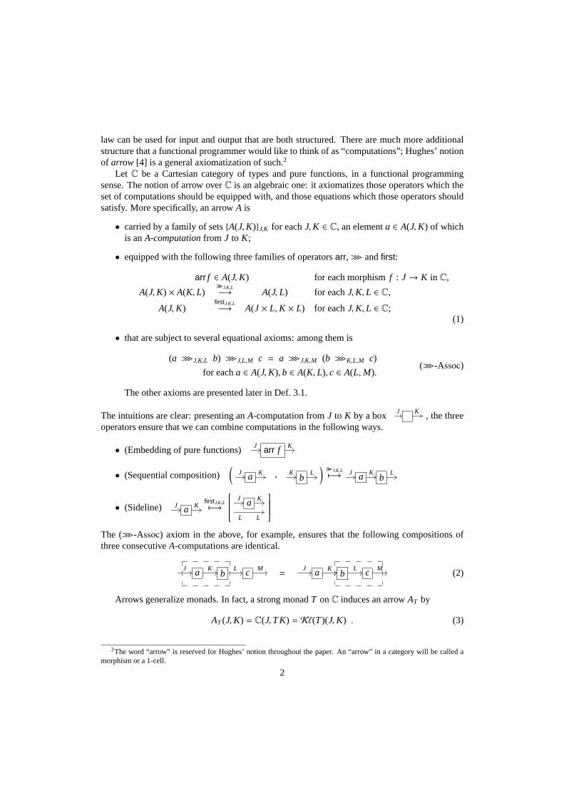
law can be used for input and output that are both structured.There are much more additionalstructure that a functional programmer would like to think of as “computations”; Hughes’ notionof arrow [4] is a general axiomatization of such.2

Let C be a Cartesian category of types and pure functions, in a functional programmingsense. The notion of arrow overC is an algebraic one: it axiomatizes those operators which theset of computations should be equipped with, and those equations which those operators shouldsatisfy. More specifically, an arrowA is

• carried by a family of sets{A(J,K)}J,K for eachJ,K ∈ C, an elementa ∈ A(J,K) of whichis anA-computationfrom J to K;

• equipped with the following three families of operatorsarr, >>> andfirst:

arr f ∈ A(J,K) for each morphismf : J→ K in C,

A(J,K) × A(K, L)>>>J,K,L−→ A(J, L) for eachJ,K, L ∈ C,

A(J,K)firstJ,K,L−→ A(J × L,K × L) for eachJ,K, L ∈ C;

(1)

• that are subject to several equational axioms: among them is

(a >>>J,K,L b) >>>J,L,M c = a >>>J,K,M (b >>>K,L,M c)

for eacha ∈ A(J,K),b ∈ A(K, L), c ∈ A(L,M).(>>>-Assoc)

The other axioms are presented later in Def. 3.1.

The intuitions are clear: presenting anA-computation fromJ to K by a boxJ K , the three

operators ensure that we can combine computations in the following ways.

• (Embedding of pure functions)J arr f K

• (Sequential composition)(

J a K , Kb

L)

>>>J,K,L7−→ J a K

bL

• (Sideline) J a KfirstJ,K,L7−→

J a K

L L

The (>>>-Assoc) axiom in the above, for example, ensures that the followingcompositions ofthree consecutiveA-computations are identical.

J a Kb

L c M=

J a Kb

L c M (2)

Arrows generalize monads. In fact, a strong monadT onC induces an arrowAT by

AT(J,K) = C(J,T K) = Kℓ(T)(J,K) . (3)

2The word “arrow” is reserved for Hughes’ notion throughout the paper. An “arrow” in a category will be called amorphism or a 1-cell.

2

HereKℓ(T) denotes the Kleisli category (see e.g. Moggi [2]). Prior toarrows, the notion ofFreyd categoryis devised as another axiomatization of algebraic properties that are expectedfrom “computations” [5, 6]. The latter notion of Freyd category comes with a stronger categoricalflavor; in Jacobs et al. [7] it is shown to be equivalent to the notion of arrow.

Remark 1.1. What has been said is true as long as we think of an arrow as carried by sets, i.e.with A(J,K) being a set. This is our setting. However this is not an entirely satisfactory viewin functional programming where one seesA as a type constructor—A(J,K) should rather be anobject ofC. In this case one can think of several variants of arrow and Freyd category. SeeAtkey [8]. The discussion later in§5.1 is also relevant.

1.2. Arrow as Component Calculus

The current paper’s goal is to settlecomponentsascategorificationof computations, via (thealgebraic theory of) arrows. Let us elaborate on this slogan.

A component here is in the sense ofcomponent calculi. Components are systems which,combined with one another by some component calculus, yielda bigger, more complicated sys-tem. This “divide-and-conquer” strategy brings order to design processes of large-scale systemsthat are otherwise messed up due to the very scale and complexity of the systems to be designed.

We follow the monad-based coalgebraic modeling of components in Barbosa [9]—whichis also used in Hasuo et al. [10]—and extend it later to an arrow-based modeling. In [9] acomponent is modeled as a coalgebra of the following type:

c : X −→(

T(X × K))J in Sets. (4)

HereJ is the set of possible input to the component;K is that of possible output;X is the set of(internal) states of the component which is a state-based machine; andT is a monad onSetsthatmodels the computational effect exhibited by the system. Overall, a coalgebraic component is astate-based system with specified input and output ports; itcan be drawn asJ c K .

A crucial observation here is as follows. The notion of arrowin §1.1 axiomatizes algebraic

operators on computations as boxes—such as sequential composition J a Kb

L . Then, by

regarding such boxes as components rather than as computations, we can employ the same ax-iomatization of arrow as algebraic structure on components—acomponent calculus—with whichone can compose components. The calculus is a basic one that allows embedding of pure func-tions, sequential composition and sideline. In fact in the first author’s previous work [10] withHeunen, Jacobs and Sokolova, such algebraic operators on coalgebraic components (4) are de-fined and shown to satisfy the equational axioms.

1.3. Categorifying Computations into Components

Despite the similarity between computations and components that we have just described,there is one level gap between them: fromsetsto categories. LetA(J,K) denote the collectionof coalgebraic components like in (4), with input-typeJ, output-typeK and fixed effectT, butwith varying state spacesX. Then it is just natural to include morphisms between coalgebrasin the overall picture, as behavior-preserving maps (see e.g. Rutten [11]) between components.HenceA(J,K) is now acategory, specifically that of

(

T( × K))J-coalgebras. In contrast, with

respect to computations there is no general notion of morphism between them, so the collectionA(J,K) of A-computations is aset.

3

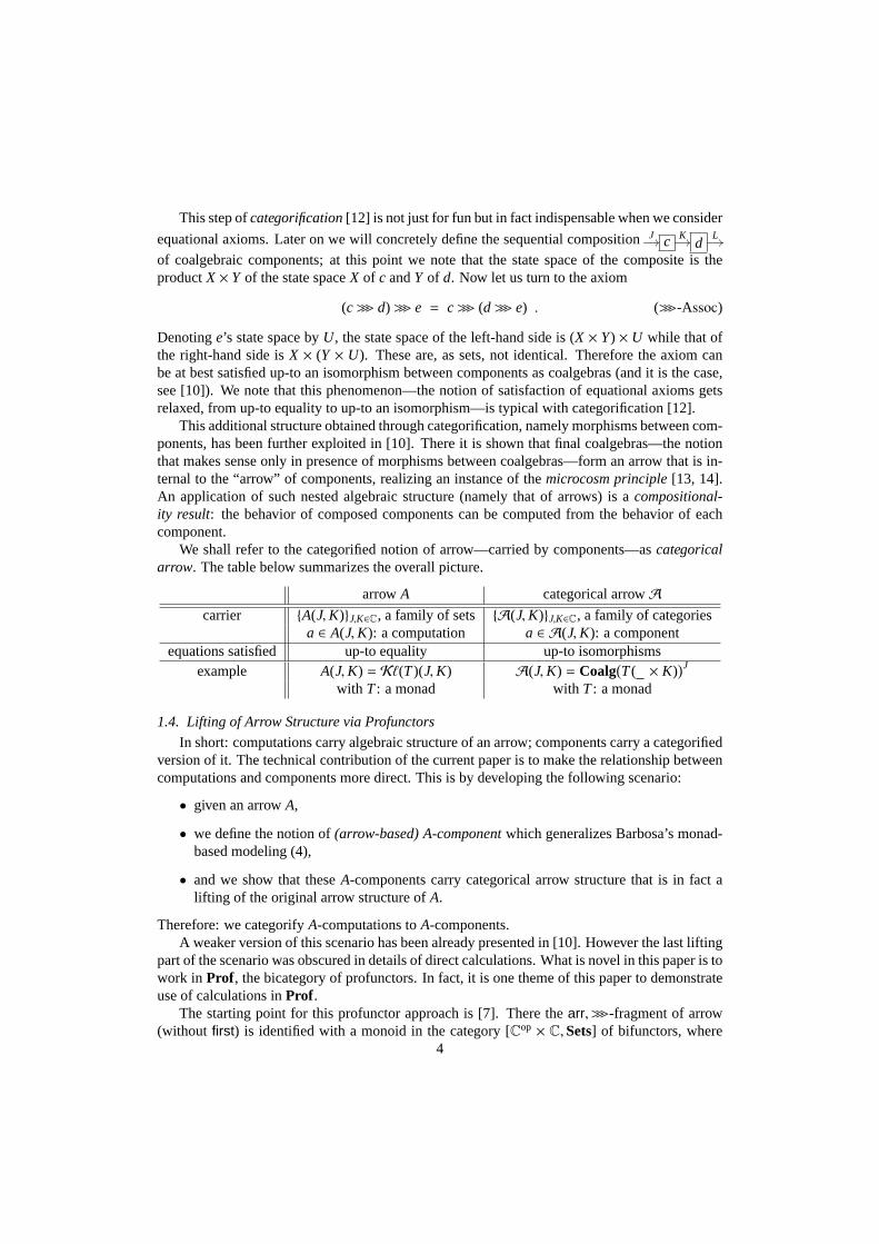
This step ofcategorification[12] is not just for fun but in fact indispensable when we consider

equational axioms. Later on we will concretely define the sequential compositionJ c Kd

L

of coalgebraic components; at this point we note that the state space of the composite is theproductX × Y of the state spaceX of c andY of d. Now let us turn to the axiom

(c>>> d) >>> e = c>>> (d >>> e) . (>>>-Assoc)

Denotinge’s state space byU, the state space of the left-hand side is (X × Y) × U while that ofthe right-hand side isX × (Y × U). These are, as sets, not identical. Therefore the axiom canbe at best satisfied up-to an isomorphism between componentsas coalgebras (and it is the case,see [10]). We note that this phenomenon—the notion of satisfaction of equational axioms getsrelaxed, from up-to equality to up-to an isomorphism—is typical with categorification [12].

This additional structure obtained through categorification, namely morphisms between com-ponents, has been further exploited in [10]. There it is shown that final coalgebras—the notionthat makes sense only in presence of morphisms between coalgebras—form an arrow that is in-ternal to the “arrow” of components, realizing an instance of the microcosm principle[13, 14].An application of such nested algebraic structure (namely that of arrows) is acompositional-ity result: the behavior of composed components can be computed from the behavior of eachcomponent.

We shall refer to the categorified notion of arrow—carried by components—ascategoricalarrow. The table below summarizes the overall picture.

arrowA categorical arrowA

carrier {A(J,K)}J,K∈C, a family of sets {A(J,K)}J,K∈C, a family of categoriesa ∈ A(J,K): a computation a ∈ A(J,K): a component

equations satisfied up-to equality up-to isomorphismsexample A(J,K) = Kℓ(T)(J,K) A(J,K) = Coalg

(

T( × K))J

with T: a monad with T: a monad

1.4. Lifting of Arrow Structure via Profunctors

In short: computations carry algebraic structure of an arrow; components carry a categorifiedversion of it. The technical contribution of the current paper is to make the relationship betweencomputations and components more direct. This is by developing the following scenario:

• given an arrowA,

• we define the notion of(arrow-based) A-componentwhich generalizes Barbosa’s monad-based modeling (4),

• and we show that theseA-components carry categorical arrow structure that is in fact alifting of the original arrow structure ofA.

Therefore: we categorifyA-computations toA-components.A weaker version of this scenario has been already presentedin [10]. However the last lifting

part of the scenario was obscured in details of direct calculations. What is novel in this paper is towork in Prof , the bicategory of profunctors. In fact, it is one theme of this paper to demonstrateuse of calculations inProf .

The starting point for this profunctor approach is [7]. There thearr, >>>-fragment of arrow(without first) is identified with a monoid in the category [C

op × C,Sets] of bifunctors, where4

the latter is equipped with suitable monoidal structure. This means—in terms of profunctors thatwill be described in§2—that an arrowA (without first) is amonadin Prof , in an internal senselike in Street [15].

What really makes our profunctor approach feasible is a further observation by the secondauthor [16]. There the remainingfirst operator—whose mathematical nature was buried awayin its dinaturality—is identified with a certain 2-cell inProf . In fact, this 2-cell is astrengthin an internal sense. Therefore an arrow (with its full set ofoperators,arr, >>> and first) isa strong monadin Prof . This observation pleasantly parallels the informal view of arrows asgeneralization of strong monads.

1.5. Organization of the Paper

In §2 we will introduce the necessary notions of dinatural transformation, (co)end and pro-functor, in a rather leisurely pace. The two forms of the Yoneda lemma—the end- and coend-forms—are basic there. The materials there are essentially extracted from Kelly [17], which isa useful reference also in the current non-enriched (i.e.Sets-enriched) setting. In§3 we fol-low [16, 7] and identify an arrow with an internal strong monad in Prof , settingProf as ouruniverse of discourse. In§4 we generalize Barbosa’s coalgebraic components into arrow-basedcomponents. The main result—arrow-based components form a categorical arrow—is statedthere. Its actual proof is in the subsequent§5 which is devoted to manipulation of 2-cells inProf .

The current version departs from the previous workshop version [1] most notably in§5.The manipulation of 2-cells is now described in a much more structural manner, using a novelbicategoryStProf. The details that have been omitted in [1] are presented as much as the spaceallows. We also explicitly settle the problem of size (§5.1); in the previous version [1] we onlyhinted possible solutions.

2. Categorical Preliminaries

2.1. End and Coend

In the sequel we shall often encounter a functor of the typeF : Cop × C → D, where a

categoryC occurs twice with different variance. Given two suchF,G : Cop×C→ D, adinatural

transformationϕ : F ⇒ G consists of a family of morphisms inD

ϕX : F(X,X) −→ G(X,X) for eachX ∈ C

which isdinatural: for each morphismf : X→ X′ the following diagram commutes.

F (X,X)ϕX

G (X,X) G(X, f )

F (X′,X)F( f ,X)

F(X′, f )

G (X,X′)F (X′,X′)

ϕX′G (X′,X′) G( f ,X′)

(5)

Note the difference from anatural transformationψ : F ⇒ G. The latter consists of a greaternumber of morphisms inD; that is,ψX,Y : F(X,Y)→ G(X,Y) for eachX,Y ∈ C.

Two successive dinatural transformationsϕ1 : F1⇒ F2 andϕ2 : F2⇒ F3 do not necessarilycompose: dinaturality of each does not guarantee dinaturality of the obvious candidate of the

5

composition (ϕ2 ◦ ϕ1)X = (ϕ2)X ◦ (ϕ1)X. This makes it a tricky business to organize dinat-ural transformations in a categorical manner. Nevertheless, working with arrows, examples ofdinaturality abound.

Dinaturality subsumes naturality: a natural transformation ψ : F ⇒ G : C → D can bethought of as a dinatural transformation, by presenting it asψ : F ◦ π2⇒ G ◦ π2 : Cop×C→ D.Hereπ2 : C

op × C→ C is a projection.(Co)endis the notion that is obtained by replacing naturality (for (co)cones) by dinaturality,

in the definition of (co)limit. Precisely:

Definition 2.1 (End and coend).Let C,D be categories andF : Cop × C→ D be a functor.

• An endof F consists of an object∫

X∈CF (X,X) in D together withprojections

πX :(

∫

X∈CF (X,X)

)

−→ F (X,X) for eachX ∈ C

such that, for each morphismf : X→ X′ in C, the following diagram commutes.

F(X′,X′) F( f ,X′)∫

XF (X,X)

πX′

πX

F(X,X′)F(X,X) F(X, f )

In other words: the family{πX}X∈C forms a dinatural transformation from the constantfunctor∆(

∫

XF(X,X)) to the functorF. An end is defined to be a universal one among such

data: given an objectY ∈ D and a dinatural transformationϕ : ∆Y⇒ F, there is a uniquemorphismf : Y→

∫

XF (X,X) such thatπX ◦ f = ϕX for eachX ∈ C.

• A coendof F is a dual notion of an end. It consists of an object∫ X∈C

F (X,X) in D together

with coprojectionsιX : F (X,X) →∫ X

F (X,X) for eachX ∈ C. Its universality, togetherwith that of an end, can be written as follows.

f : Y −→∫

XF (X,X)

ϕX : Y→ F (X,X) , dinatural inX

f :∫ X

F (X,X) −→ Y

ϕX : F (X,X)→ Y, dinatural inX

(Co)ends need not exist; they do exist for example whenC is small andD is (co)complete. Seebelow.

The reader is referred to Mac Lane [18, Chap. IX] for more on (co)ends. Described there isthe way to transform a functorF : C

op × C → D into F§ : C§ → D, in such a way that the

(co)end ofF coincides with the (co)limit ofF§. Therefore existence of (co)ends depends on the(co)completeness property ofD. In fact (co)end subsumes (co)limit, just as dinaturality subsumesnaturality. Therefore a useful notational convention is todenote (co)limits also as (co)ends: forexample ColimXFX as

∫ XFX.

Recalling the construction of any limit by a product and an equalizer [18,§V.2], an intuitionabout an end

∫

XF(X,X) is as follows: it is the product

∏

X F(X,X) which is “cut down” so as to

satisfy dinaturality. Dually, a coend∫ X

F(X,X) is the coproduct∐

X F(X,X) quotiented modulodinaturality.

6

2.2. Two Forms of the Yoneda Lemma

A typical example of an end arises as a set of (di)natural transformations. Given a smallcategoryC and functorsF,G : C

op × C→ Sets, we obtain a bifunctor

[F(+,−),G(−,+)] : Cop × C −→ Sets , (X,Y) 7−→ [F(Y,X),G(X,Y)] . (6)

Here [S,T] denotes the set of functions fromS to T, i.e. an exponential inSets. Note thevariance: since [−,+] is contravariant in its first argument, the variance of arguments ofF isopposed in (6). Taking this functor (6) asF in Def. 2.1, we define an end

∫

X[F(X,X),G(X,X)].

Such an end does exist whenC is a small category, becauseSetshas small limits (hence smallends).

Proposition 2.2. Let us denote the set of dinatural transformations from F to Gby Dinat(F,G).We have a canonical isomorphism inSets:

Dinat(F,G)�

−→∫

X[F(X,X),G(X,X)] .

Proof. It is due to the following correspondences.

1→∫

X[F (X,X) ,G (X,X)]

1→ [F (X,X) ,G (X,X)] , dinatural inX(†)

F (X,X)→ G (X,X) , dinatural inX(‡)

Here (†) is by Def. 2.1; dinaturality is preserved along (‡) because of the naturality of Currying.2

The composite Dinat(F,G)�

→∫

X[F(X,X),G(X,X)]

πX−→ [F(X,X),G(X,X)] carries a dinatural

transformationϕ to its X-componentϕX.Since dinaturality subsumes naturality (§2.1), we have an immediate corollary:

Corollary 2.3. Let C be a small category and F,G : C → Sets. ByNat(F,G) we denote the setof natural transformations F⇒ G. We have

Nat(F,G)�

−→∫

X[FX,GX] . 2

The celebratedYoneda lemmareduces the set Nat(C(X, ), F) of natural transformations intoFX (see e.g. [18, 19]). Interpreted via Cor. 2.3, it yields:

Lemma 2.4 (The Yoneda lemma, end-form).Given a small categoryC and a functor F: C→

Sets, we have a canonical isomorphism

∫

X′∈C[C (X,X′) , FX′]

�

−→ FX . 2

The lemma becomes useful in the calculations below: it meansan end on the left-hand side“cancels” with a hom-functor occurring in it.

From the end-form, we obtain the following coend-form. Its proof is straightforward butilluminating. It allows us to “cancel” a coend with a hom-functor inside it.

7

Lemma 2.5 (The Yoneda lemma, coend-form).Given a small categoryC and a functor F :C→ Sets, we have a canonical isomorphism

∫ X′∈CFX′ × C(X′,X)

�

−→ FX .

Proof. We have the following canonical isomorphisms, for eachS ∈ Sets.

[

∫ X′FX′ × C(X′,X) , S

]

�→∫

X′[

FX′ × C(X′,X) , S]

(†)�→∫

X′[

C(X′,X) , [FX′,S]]

Currying�→ [FX,S] the Yoneda lemma, end-form.

Here (†) is because the hom-functor [,S] turns a colimit into a limit [18,§V.4], hence a coendinto an end. Obviously the composite isomorphism is naturalin S; therefore we have shown that

y(

∫ X′C(X′,X) × FX′

) �

−→ y(FX) : C −→ Sets , (7)

wherey : Cop → [C,Sets] is the (contravariant) Yoneda embedding. By the Yoneda lemma thefunctory is full and faithful; therefore it reflects isomorphisms. Hence (7) proves the claim.2

2.3. ProfunctorDefinition 2.6 (Profunctor). Let C andD be small categories. Aprofunctor Pfrom C to D is afunctorP : D

op × C→ Sets. It is denoted byP : C p→ D. That is,

C p−→ D, a profunctor

Dop × C −→ Sets, a functor

The notion of profunctor is also calleddistributor, bimoduleor module. For more detailed treat-ment of profunctors see e.g. Benabou [20] and Borceux [21].

There are two principal ways to understand profunctors. Oneis as “generalized relations”:profunctors are to functors what relations are to functions. The differences between a profunctorP : C p→ D and a relationR : S p→ T are as follows.

• A relation is two-valued: for each elements ∈ S and t ∈ T, R(s, t) is either empty (i.e.(s, t) < R) or filled (i.e. (s, t) ∈ R). In contrast, a profunctor is valued with arbitrary sets,that is,P(Y,X) ∈ Sets.

• The functoriality of a profunctorP inducesaction of morphisms inC and D. For il-

lustration let us depict an elementp ∈ P(Y,X) by a box Y p X . Given two mor-phismsg : Y′ → Y in D and f : X → X′ in C, functoriality of P yields an elementP(g, f )(p) ∈ P(Y′,X′) (note the variance); the latter element is best depicted asfollows.

Y′ g Y p X f X′ (8)

The last point (“C-D-action”) motivates another way of looking at profunctors:as generalizedmodulesas in the theory of rings. These generalized modules are carried by a family of sets{P(Y,X)}X∈C,Y∈D, with left-action ofC-arrows and right-action ofD-arrows. Also notice thesimilarity between (8) and the diagrams in§1 for computations/components. It is indeed thissimilarity that allows us to formalize arrows as certain profunctors (§3).

8

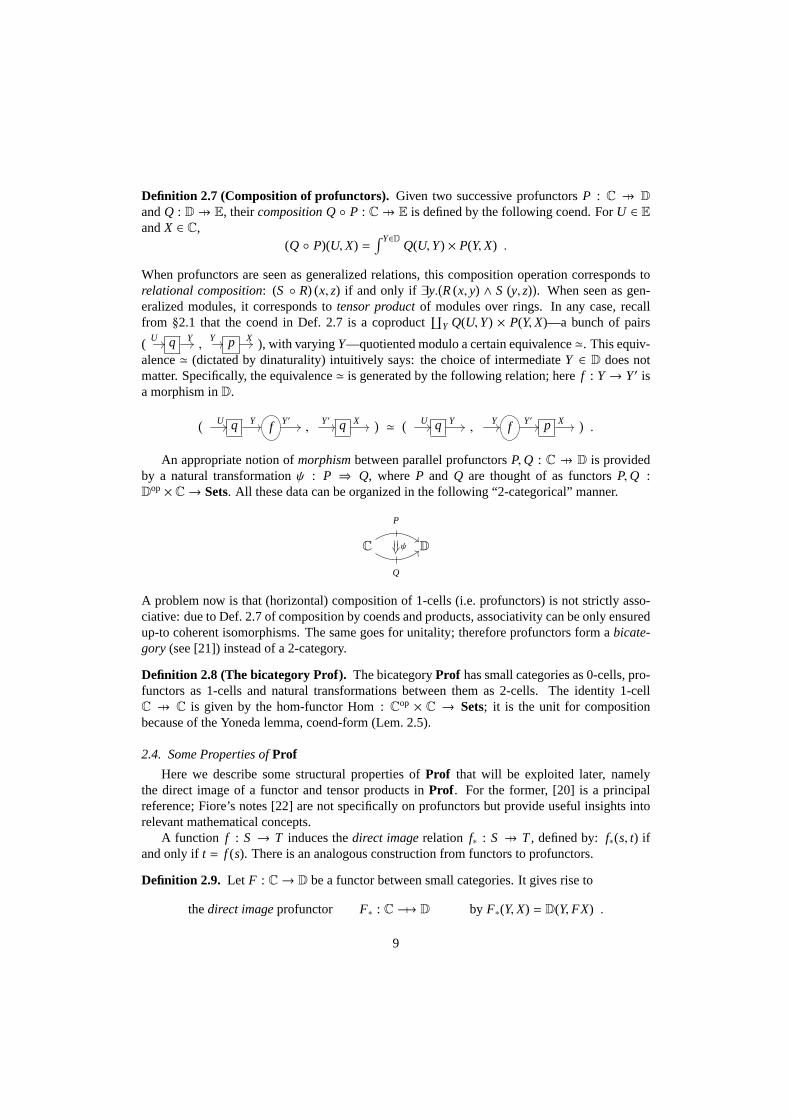
Definition 2.7 (Composition of profunctors). Given two successive profunctorsP : C p→ D

andQ : D p→ E, theircomposition Q◦ P : C p→ E is defined by the following coend. ForU ∈ E

andX ∈ C,(Q ◦ P)(U,X) =

∫ Y∈DQ(U,Y) × P(Y,X) .

When profunctors are seen as generalized relations, this composition operation corresponds torelational composition: (S ◦ R) (x, z) if and only if ∃y.

(

R(x, y) ∧ S (y, z))

. When seen as gen-eralized modules, it corresponds totensor productof modules over rings. In any case, recallfrom §2.1 that the coend in Def. 2.7 is a coproduct

∐

Y Q(U,Y) × P(Y,X)—a bunch of pairs

(U q Y

,Y p X ), with varyingY—quotiented modulo a certain equivalence≃. This equiv-

alence≃ (dictated by dinaturality) intuitively says: the choice ofintermediateY ∈ D does notmatter. Specifically, the equivalence≃ is generated by the following relation; heref : Y→ Y′ isa morphism inD.

( U q Y f Y′,

Y′ q X )

≃( U q Y

,Y f Y′ p X )

.

An appropriate notion ofmorphismbetween parallel profunctorsP,Q : C p→ D is providedby a natural transformationψ : P ⇒ Q, whereP and Q are thought of as functorsP,Q :D

op × C→ Sets. All these data can be organized in the following “2-categorical” manner.

C

P

Q

ψ D

A problem now is that (horizontal) composition of 1-cells (i.e. profunctors) is not strictly asso-ciative: due to Def. 2.7 of composition by coends and products, associativity can be only ensuredup-to coherent isomorphisms. The same goes for unitality; therefore profunctors form abicate-gory (see [21]) instead of a 2-category.

Definition 2.8 (The bicategory Prof). The bicategoryProf has small categories as 0-cells, pro-functors as 1-cells and natural transformations between them as 2-cells. The identity 1-cellC p→ C is given by the hom-functor Hom :Cop × C → Sets; it is the unit for compositionbecause of the Yoneda lemma, coend-form (Lem. 2.5).

2.4. Some Properties ofProf

Here we describe some structural properties ofProf that will be exploited later, namelythe direct image of a functor and tensor products inProf . For the former, [20] is a principalreference; Fiore’s notes [22] are not specifically on profunctors but provide useful insights intorelevant mathematical concepts.

A function f : S → T induces thedirect imagerelation f∗ : S p→ T, defined by: f∗(s, t) ifand only ift = f (s). There is an analogous construction from functors to profunctors.

Definition 2.9. Let F : C→ D be a functor between small categories. It gives rise to

thedirect imageprofunctor F∗ : C p−→ D by F∗(Y,X) = D(Y, FX) .

9

The mapping ( )∗ also applies to natural transformations in an obvious way; this determines apseudo functor(see e.g. [21]) ( )∗ : Cat→ Prof that embedsCat in Prof .

Notations 2.10. Throughout the rest of the paper, the direct imageF∗ of a functorF shall besimply denoted byF. The identity profunctor id :C p→ C—that is the hom-functor—will beoften denoted byC : C p→ C.

The Cartesian product operator× in Cat lifts Prof : given profunctorsF : C p→ C′ and

G : D p→ D′, we define

F ×G : C × D p→ C′ × D

′ by (F ×G)(X′,Y′,X,Y) = F(X′,X) ×G(Y′,Y) . (9)

The symbol× occurring in the last denotes the Cartesian product inSets. The lifted operator× inProf makes it a “monoidal bicategory,” a notion whose precise definition involves delicate han-dling of coherence. We shall not do that in this paper. Nevertheless, we will need the followingproperty.

Lemma 2.11. The operation× onProf is bifunctorial: that is, given four profunctorsCPp→ D

Qp→

E andC′

P′

p→ D′

Q′

p→ E′ we have(Q ◦ P) × (Q′ ◦ P′) �→ (Q× Q′) ◦ (P× P′).

Proof. This is due to the Fubini theorem for coends. See [18,§IX.8] 2

It is obvious that the operator× acts also on 2-cells (that are natural transformations).

3. Arrows as Profunctors

We review the results in [7, 16] that identify Hughes’ notionof arrow with a profunctor withadditional algebraic structure.

First we present the precise definition of arrow. Usually it is defined over a Cartesian categoryC. However, since it is rather the monoidal structure ofC that is essential, we shall work with amonoidal category.

Definition 3.1 (Arrow [4]). Given a monoidal categoryC = (C,⊗, I ), anarrow overC consistsof carrier sets{A(J,K)}J,K∈C and operatorsarr, >>> andfirst as described in (1). The operatorsmust satisfy the following equational axioms.

(a>>> b) >>> c = a>>> (b>>> c) (>>>-Assoc)arr (g ◦ f ) = arr f >>> arr g (arr-Func1)

arr idJ >>>J,J,K a = a = a>>>J,K,K arr idK (arr-Func2)firstJ,K,I a >>> arr ρK = arr ρK >>> a (ρ-Nat)

firstJ,K,L a >>> arr(idK ⊗ f ) = arr(idJ ⊗ f ) >>> firstJ,K,M a (arr-Centr)(arrαJ,L,M) >>> (firstJ,K,L⊗M a) = first(first a) >>> (arrαK,L,M) (α-Nat)

firstJ,K,L(arr f ) = arr( f ⊗ idL) (arr-Premon)firstJ,L,M(a>>> b) = (firstJ,K,M a) >>> (firstK,L,M b) (first-Func)

Here some subscripts are suppressed. The morphismρK : K ⊗ I �→ K is the right unitalityisomorphism;αK,L,M : (K ⊗ L)⊗M �→ K ⊗ (L⊗M) is the associativity isomorphism. The namesof the axioms hint their correspondence to the (premonoidal) structure ofFreyd categories[5, 6].

10

Next we introduce the corresponding construct inProf , which we shall tentatively call aProf -arrow.

Definition 3.2 (Prof-arrow). Let C = (C,⊗, I ) be a small monoidal category. AProf -arrowoverC is:

• a profunctorA : C p→ C,

• equipped with natural transformationsarr, >>>, first of the following types:

C

C

A

⇓ arr C ,C

A

A

⇓>>>

CA

C,

C2 A×C

⊗ ⇓ firstC

2

⊗

CA

C

,

where all the diagrams are inProf ,

• subject to the equalities in Table 1. Recall Notations 2.10;for example the profunctor〈C, I〉 in (first-ρ) is the functor〈C, I〉 : C → C

2, X 7→ (X, I ), embedded inProf by takingits direct image.

The notion ofProf -arrow is in fact a familiar one: it is astrong monadin Prof , definedinternally in the sense of [15]. This means the following. When one draws the same 2-cellsin Cat instead of inProf—replacingA by T, arr by ηT , >>> by µT andfirst by str′—the defi-nition coincides with that of strong monad [23, 2].3 More specifically, the first two axioms inTable 1 are for the monad laws; and the remaining axioms asserts compatibility of strength withmonoidal and monad structure. For example, the axiom (first->>>) interpreted inCat is read asthe commutativity of the following diagram.

T2X ⊗ Ystr′

µT⊗Y

T(T X⊗ Y) Tstr′T2(X ⊗ Y)

µT

T X⊗ Ystr′

T(X ⊗ Y)

(Internal) strong monads can be defined in any bicategory with suitable monoidal structure. Laterin §5 we introduce a bicategoryStProf; strong monads therein play an important role.

Proposition 3.3 ([16]). For a monoidal categoryC that is small, the notion of arrow (Def. 3.1)and that ofProf -arrow (Def. 3.2) are equivalent.

Proof. While the reader is referred to [16] for a detailed proof, we present a few highlights in thecorrespondence between the two notions. We shall writearr′, >>>′ andfirst′ (with primes) for thethree operators of aProf -arrow (Def. 3.2), to distinguish them from the corresponding operatorsof an arrow (Def. 3.1).

3The corresponding strength operatorstr′ is of the typestr′ : T X⊗Y→ T(X⊗Y), which is slightly different from theusual strength operator that isstr : X⊗TY→ T(X⊗Y). These two are equivalent when the base categoryC is symmetricmonoidal.

11

C

C

arr

A

A

>>>C

AC = C

A

A

id C = CA

A

>>>C

C

arr

AC (Unit)

CA

A

⇓>>>

CA

A

>>>C

AC

=

CA

A

⇓>>>A

>>>C

AC

AC

(Assoc)

C3 A×C×C

⊗×C

C×⊗⇓ first×C

C3

⊗×C

C2

⊗

⇐�

α C2

⊗A×C

⇓ first

C2

⊗

CA

C

=

C3 A×C×C

C×⊗

C3

C×⊗⊗×C

C2

⊗A×C

⇓ first

C2

⊗

⇐�

α C2

⊗

CA

C

(first-α)

C〈C,I〉

C

ρ ⇓�C

2 A×C

⊗ ⇓ first

C2

⊗

CA

C

=

C〈C,I〉

A

C2 A×C

C2

⊗

CC

ρ ⇓�

〈C,I〉

C

(first-ρ)

C2

C×C

arr×C

A×C

⊗ ⇓ first

C2

⊗

CA

C

= C2 ⊗C

C

A

arr C (first-arr)

C2 A×C

⇓ first⊗

C2 A×C

⇓ first⊗

C2

⊗

CA

A

>>>C

AC =

C2 A×C

A×C

>>>×C

⊗

C2 A×C

C2

⊗

CA

⇓ first

C

(first->>>)

Table 1: Equational axioms forProf -arrow

12

Let us first observe that a 2-cellfirst′ in Prof gives rise to thefirst operator in Def. 3.1. Theformer is an element of the left-hand side below, where◦ denotes composition of profunctors(Def. 2.7).

Nat(

(⊗ ◦ (A× C))(−,+1,+2) , (A ◦ ⊗)(−,+1,+2))

�∫

X,K,Y∈C

[

(⊗ ◦ (A× C))(X,K,Y) , (A ◦ ⊗)(X,K,Y)]

by Cor. 2.3

�∫

X,K,Y

[

∫ J,LC(X, J ⊗ L) × A(J,K) × C(L,Y) ,

∫ UA(X,U) × C(U,K ⊗ Y)

]

by Def. 2.7, Def. 2.9 and (9)

�∫

X,K,Y,J,L

[

C(X, J ⊗ L) × A(J,K) × C(L,Y) ,∫ U

A(X,U) × C(U,K ⊗ Y)]

since a hom-functor [−,S] turns a coend into an end

�∫

X,K,Y,J,L

[

C(X, J ⊗ L),[

A(J,K),[

C(L,Y) ,∫ U

A(X,U) × C(U,K ⊗ Y)]]]

by Currying

�∫

J,K,L

[

A(J,K), A(J ⊗ L,K ⊗ L)]

by cancelingX,Y by Lem. 2.4 andU by Lem. 2.5

� NatJ,KDinatL(

A(J,K), A(J ⊗ L,K ⊗ L))

by Prop. 2.2 and Cor. 2.3.

Therefore a 2-cellfirst′ in Prof gives rise to a family of functionsA(J,K)→ A(J⊗ L,K ⊗ L) thatis natural inJ,K and dinatural inL. This is precisely the type of thefirst operator in Def. 3.1. Theequational axioms of an arrow are indeed satisfied due to those of aProf -arrow. We note that theaxiom (arr-Centr) is satisfied not because of any specific axiom of aProf -arrow, but because ofthe dinaturality offirst′ as a 2-cell inProf .

For the opposite direction where an arrow induces aProf -arrow, we have to equip the carrier{A(J,K)}J,K of an arrow with action of morphisms inC, renderingA into a functorCop × C →

Sets. This is done with the help of arrow operators. Specifically,A(g, f )(a) := arr f >>>a>>>arrg,that is:

Y′f

Ya

X g X′ := Y′arr f

Ya

X arrg X′ .

Each of the arrow operators yields its correspondingProf -arrow operator; the latter’s (di)naturalityis derived from the arrow axioms. So are the equational axioms for aProf -arrow. 2

Prop. 3.3 offers a novel mathematical understanding of the notion of arrow. It endows the seem-ingly complicated original axiomatization (Def. 3.1) withcategorical canonicity. Its treatment offirst as a strength also seems simpler than that in Freyd categories: the latter involves technical-ities like premonoidal categories and central morphisms. It is this simplicity that is exploited inthe rest of the paper.

Remark 3.4. A size issue about Prop. 3.3 should be noted. While the original definition of arrow(Def. 3.1) makes sense for any base categoryC without size restriction, its characterization inProf (Def. 3.2) requiresC be small. Without the restriction the compositionA ◦ A—the domainof the 2-cell>>> in Prof—is not necessarily well-defined:A ◦ A is defined via coends inSets(Def. 2.7) andSetsis only small-complete. This becomes a real obstacle later where we consideran arrowA overC = Setswhich is not small. We shall fix this problem by “upgrading” the sizeof profunctors; see§5.1.

When the base monoidal categoryC is symmetric—which is our setting in the sequel—wecan obtain another sideline operatorsecond.

13

Definition 3.5. Let A be an arrow over a small symmetric monoidal category (SMC)C. Wedefine an extra operatorsecond as the following 2-cell inProf .

C2 C×A

⊗ ⇓ secondC

2

⊗

CA

C

:=

C2 C×A

〈π2,π1〉

⊗�⇐σ−1

C2

〈π2,π1〉

⊗�⇐σC

2 A×C

⊗ ⇓ firstC

2

⊗

CA

C

(10)

Here the profunctor〈π2, π1〉 is the direct image of the functor〈π2, π1〉 : C2→ C

2, mapping (X,Y)to (Y,X) (cf. Notations 2.10). The 2-cellσ is the symmetry isomorphismσX,Y : X ⊗ Y �→ Y⊗ X.

Notations 3.6. In the above diagrams as well as elsewhere, there appear two different classes ofiso 2-cells inProf . One class is due to the unitality/associativity/symmetry of⊗ on a monoidalbase categoryC; they are iso 2-cells inCat embedded inProf via direct image (§2.4). Such iso2-cells shall be filled explicitly with the� sign, like the two on the right-hand side in (10).

The other class is due to the properties of the operation× onProf , typically Lem. 2.11. Suchiso 2-cells will be denoted by empty polygons, like the top one on the right-hand side in (10).

Some calculations like in the proof of Prop. 3.3 reveal that this new operator realizes a class

of functionsA(J,K)secondJ,K,L−→ A(L × J, L × K), that is graphically

J a KsecondJ,K,L7−→

L L

Ja

K

:=

J a K

L L

.

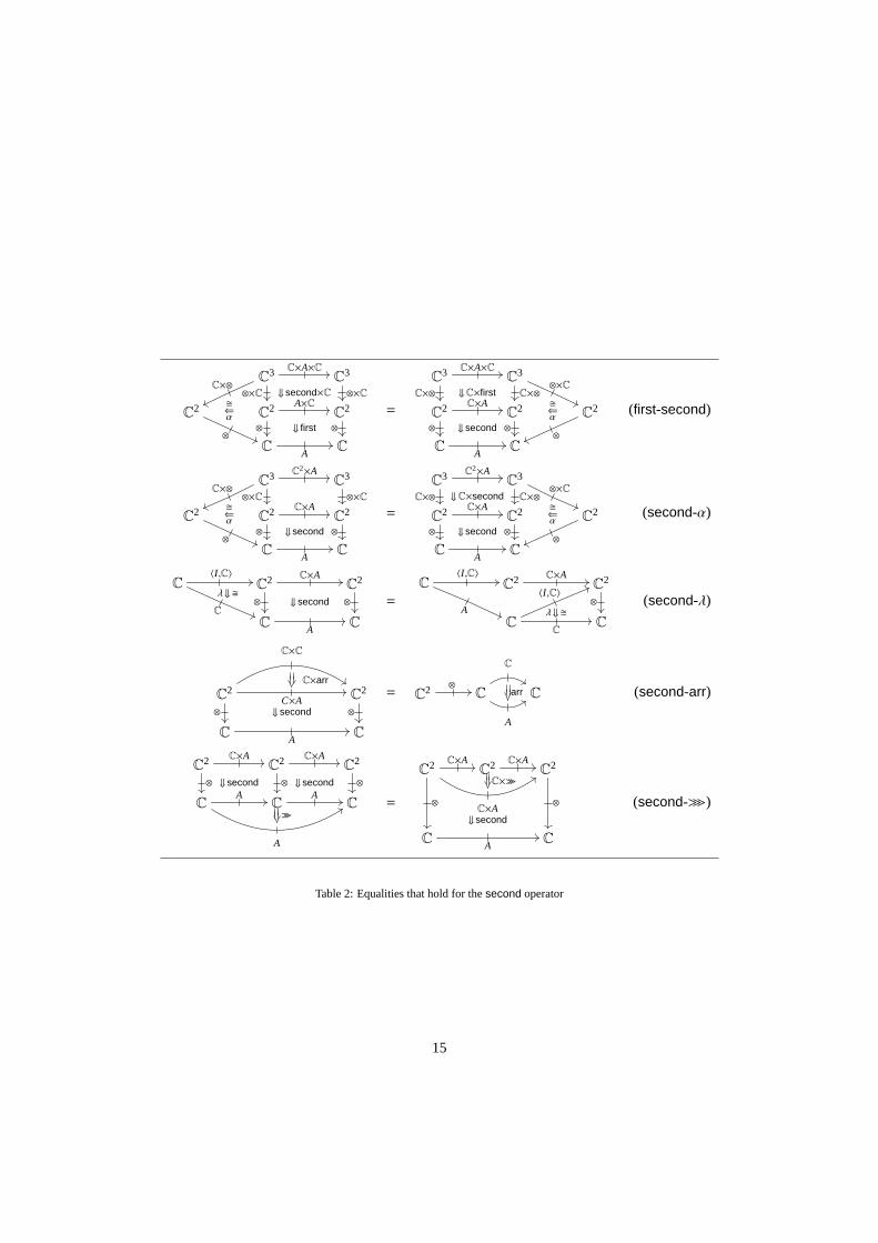
Lemma 3.7. Regarding thesecond operator, the equalities in Table 2 hold.

Proof. Use (first-α), (first-arr), (first-ρ), (first->>>) in Table 1 and the coherence for an SMCC.2

4. Arrow-Based Components

4.1. Main ContributionIn this section we develop the scenario in§1.4 in technical terms. First we introduce an

arrow-based coalgebraic modeling of components.

Definition 4.1 (A-component). Let A be an arrow overSets, andJ,K ∈ Sets. An (arrow-based)A-componentwith input-typeJ, output-typeK and computational structureA is a coalgebra forthe functorA(J, × K) : Sets→ Sets. That is,

J c K asA(J,X × K)

Xc .

Here an arrowA is in the sense of Def. 3.1. In Def. 3.1 the base categoryC of an arrow need notbe small; thus we choose (Sets,×,1) asC. Our modeling specializes to Barbosa’s (4) when wetake asA a monad-based arrowAT in (3). Our modeling not only generalizes Barbosa’s but alsobrings conceptual clarity to the subsequent technical development.

Our goal is to lift the arrow structure ofA to the categorical arrow structure ofA-components.Let us state this goal precisely.

14

C3 C×A×C

⊗×CC×⊗

⇓ second×C

C3

⊗×C

C2

⊗

⇐�

α C2 A×C

⊗ ⇓ firstC

2

⊗

CA

C

=

C3 C×A×C

C×⊗ ⇓C×first

C3

C×⊗⊗×C

C2 C×A

⊗ ⇓ secondC

2

⊗

⇐�

α C2

⊗

CA

C

(first-second)

C3 C

2×A

⊗×CC×⊗

C3

⊗×C

C2

⊗

⇐�

α C2 C×A

⊗ ⇓ secondC

2

⊗

CA

C

=

C3 C

2×A

C×⊗ ⇓C×second

C3

C×⊗⊗×C

C2 C×A

⊗ ⇓ secondC

2

⊗

⇐�

α C2

⊗

CA

C

(second-α)

C〈I ,C〉

C

λ ⇓�C

2 C×A

⊗ ⇓ second

C2

⊗

CA

C

=

C〈I ,C〉

A

C2 C×AC2

⊗

CC

λ ⇓�

〈I ,C〉

C

(second-λ)

C2

C×C

C×arr

C×A⊗ ⇓ second

C2

⊗

CA

C

= C2 ⊗

C

C

A

arr C (second-arr)

C2 C×A

⇓ second⊗

C2 C×A

⇓ second⊗

C2

⊗

CA

A

>>>C

AC =

C2 C×A

C×A

C×>>>

⊗

C2 C×A

C2

⊗

CA

⇓ second

C

(second->>>)

Table 2: Equalities that hold for thesecond operator

15

Definition 4.2 (Categorical arrow). A categorical arrowconsists of

• a family {A(J,K)}J,K of carrier categories, one for eachJ,K ∈ Sets;

• (interpretation of) arrow operatorsarr, >>> andfirst (cf. Def. 3.1), namely functors

1arr f−→ A(J,K) for each functionf : J→ K in Sets,

A(J,K) ×A(K, L)>>>J,K,L−→ A(J, L) for eachJ,K, L ∈ Sets,

A(J,K)firstJ,K,L−→ A(J × L,K × L) for eachJ,K, L ∈ Sets.

Here the category1 is the one-object and one-arrow (i.e. terminal) category; and

• the operators are subject to the arrow axioms in Def. 3.1, up-to isomorphisms. For exam-ple, as to the axiom (>>>-Assoc), the following diagram must commute up-to an isomor-phism.

A(J,K) ×A(K, L) ×A(L,M)>>>J,K,L×id

id×>>>K,L,M ⇓�

A(J, L) ×A(L,M)>>>J,L,M

A(J,K) ×A(K,M)>>>J,K,M

A(J,M)(11)

The graphical understanding of a categorical arrow is the same as that of an arrow; see§1.1.In §1.3 we described why it is natural and necessary to require the axioms be satisfied only up-toisomorphisms.

Remark 4.3. Satisfaction up-to isomorphisms raises acoherenceissue. The precise coherencecondition for categorical arrows is described in [10], in a more general form of coherence forcategorical models of FP-theories. Although we shall not further discuss the coherence issue, thecalculations later in§5 provide us a much better grip on it than the direct calculations in [10] do.

The notion of categorical arrow in Def. 4.2 could be formalized on any monoidal categoryCother thanSets. We do not need such additional generality.

The main contribution of this paper is the following result as well as its proof presented inthe rest of the paper.

Theorem 4.4 (Main result). Let A be an arrow overSets. The categories{Coalg(A(J, × K) )}J,Kof A-components carry a categorical arrow.

One use of the theorem is as follows. We can appeal to the formalization [14, 10] of themicro-cosm principle[13] to obtain the followingcompositionality result.

Corollary 4.5 (Compositionality). In the setting of Thm. 4.4, assume further that for eachJ,K ∈ Setsthe functor A(J, × K) has a final coalgebraζJ,K : ZJ,K

�→ A(J,ZJ,K × K).

1. The family{ZJ,K}J,K of sets carries canonical arrow structure. This gives us e.g. “compo-sition of behaviors”

ZJ,K × ZK,L>>>Z

−→ ZJ,L .

16

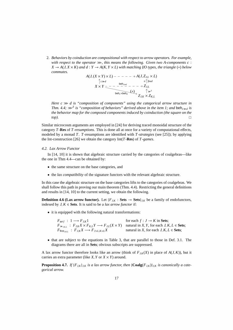
2. Behaviors by coinduction are compositional with respect toarrow operators. For example,with respect to the operator>>>, this means the following. Given two A-components c:X→ A(J,X × K) and d: Y→ A(K,Y× L) with matching I/O types, the triangle(∗) belowcommutes.

A(J, (X × Y) × L) A(J,ZJ,L × L)

X × Yc>>>d

behc>>>d

(∗)behc×behd

ZJ,L

� final

ZJ,K × ZK,L

>>>Z

Here c>>> d is “composition of components” using the categorical arrow structure inThm. 4.4;>>>Z is “composition of behaviors” derived above in the item 1; and behc>>>d isthe behavior map for the composed components induced by coinduction (the square on thetop). 2

Similar microcosm arguments are employed in [24] for deriving traced monoidal structure of thecategoryT-Resof T-resumptions. This is done all at once for a variety of computational effects,modeled by a monadT. T-resumptions are identified withT-strategies(see [25]); by applyingthe Int-construction [26] we obtain the category Int(T-Res) of T-games.

4.2. Lax Arrow Functor

In [14, 10] it is shown that algebraic structure carried by the categories of coalgebras—likethe one in Thm 4.4—can be obtained by:

• the same structure on the base categories, and

• the lax compatibilityof the signature functors with the relevant algebraic structure.

In this case the algebraic structure on the base categories lifts to the categories of coalgebras. Weshall follow this path in proving our main theorem (Thm. 4.4). Restricting the general definitionsand results in [14, 10] to the current setting, we obtain the following.

Definition 4.6 (Lax arrow functor). Let {FJ,K : Sets→ Sets}J,K be a family of endofunctors,indexed byJ,K ∈ Sets. It is said to be alax arrow functorif:

• it is equipped with the following natural transformations:

Farr f : 1 −→ FJ,K1 for eachf : J→ K in Sets;F>>>J,K,L : FJ,KX × FK,LY −→ FJ,L(X × Y) natural inX,Y, for eachJ,K, L ∈ Sets;FfirstJ,K,L : FJ,KX −→ FJ×L,K×LX natural inX, for eachJ,K, L ∈ Sets;

• that are subject to the equations in Table 3, that are parallel to those in Def. 3.1. Thediagrams there are all inSets; obvious subscripts are suppressed.

A lax arrow functor therefore looks like an arrow (think ofFJ,K(X) in place ofA(J,K)), but itcarries an extra parameter (likeX,Y or X × Y) around.

Proposition 4.7. If {FJ,K}J,K is a lax arrow functor, then{Coalg(FJ,K)}J,K is canonically a cate-gorical arrow.

17

FJ,K X × FK,LY× FL,MU

(>>>-Assoc)id×F>>>

F>>>×id

FJ,K X × FK,M(Y× U)

F>>>FJ,L(X × Y) × FL,MUF>>>

FJ,M((X × Y) × U) � FJ,M(X × (Y× U))

1

(arr-Func1)

Farr(g◦ f )〈Farr f ,Farrg〉

FJ,K1× FK,L1F>>>

FJ,L(1× 1) � FJ,L1

FJ,K X

(arr-Func2)〈id,Farr idK

〉

〈Farr idJ,id〉

id

FJ,K X × FK,K1F>>>

FJ,J1× FJ,K XF>>>

FJ,K(X × 1)�

FJ,L(1× X) � FJ,K X

FJ,K X

(ρ-Nat)〈Farr π1 ,id〉

Ffirst

FJ×1,J1× FJ,K XF>>>

FJ×1,K×1X〈id,Farr π1 〉

FJ×1,K(1× X)

�FJ×1,K×1X × FK×1,K1F>>>

FJ×1,K(X × 1) � FJ×1,K X

FJ,K X

(arr-Centr)Ffirst

Ffirst

FJ×L′ ,K×L′X

〈Farr(J× f ) ,id〉

FJ×L,K×LX

〈id,Farr(K× f )〉

FJ×L,J×L′1×FJ×L′ ,K×L′X

F>>>

FJ×L,K×LX×FK×L,K×L′1

F>>>

FJ×L,K×L′ (1× X)

�FJ×L,K×L′ (X × 1)

�

FJ×L,K×L′X

FJ,K X

(α-Nat)Ffirst

Ffirst

FJ×L,K×LXFfirst

FJ×(L×M),K×(L×M)X〈id,Farrα〉

F(J×L)×M,(K×L)×MX〈Farrα ,id〉

FJ×(L×M),K×(L×M)X×FK×(L×M),(K×L)×M1

F>>>

FJ×(L×M),(J×L)×M1×F(J×L)×M,(K×L)×MX

F>>>

FJ×(L×M),(K×L)×M(1× X)�

FJ×(L×M),(K×L)×M(X × 1) � FJ×(L×M),(K×L)×MX

1

(arr-Premon)Farr f

Farr( f×L)

FJ,K1Ffirst

FJ×L,K×L1

FJ,K X × FK,LY

(first-Func)Ffirst×Ffirst

F>>>

FJ×M,K×MX × FK×M,L×MYF>>>

FJ,L(X × Y)Ffirst

FJ×M,L×M(X × Y)

Table 3: Equational axioms for lax arrow functors

18

Proof. This follows from a general result like [10, Thm. 4.6]. Herewe briefly illustrate what thecategorical arrow structure of{Coalg(FJ,K)}J,K looks like, by describing the sequential compo-sition>>> : Coalg(FJ,K) × Coalg(FK,L) −→ Coalg(FJ,L). UsingF>>> in Def. 4.6 it is defined asfollows.

FJ,KX

Xc ,

FK,LY

Yd

>>>7−→

FJ,L(X × Y)

FJ,KX × FK,LYF>>>

X × Yc×d

The definitions are similar for the other arrow operators. The arrow axioms are satisfied due tothe corresponding equational condition on the lax arrow functor. 2

This proposition reduces Thm. 4.4 to the fact that the family{A(J, × K)}J,K is a lax arrowfunctor. This is what will be shown in the next section, through manipulation of 2-cells inProf .

5. Calculations in Prof

5.1. The Size Issue

There is one technical problem—of a bookkeeping kind—lying infront of us: the size issue.It has been briefly discussed in Rem. 3.4. The 0-cells ofProf aresmallcategories; the smallnessrestriction is necessary for composition of profunctors tobe well-defined (Def. 2.7). However,with Setsnot being small, the arrowA in Def. 4.1 cannot be a 1-cell inProf . At the same timewe need the arrowA to be based onSetsso thatA(J, × K) is an endofunctorSets→ Sets.There are two possible ways round.

• We upgrade the size of profunctors. We use the categoryEnsof sets and classes of certainsizes, so thatEns hasSets-indexed colimits/coends. A profunctorP : C p→ D is thendefined to be a bifunctorDop × C → Ens. This upgrade is purely for the sake of abstractarguments: we will still require the arrowA to be “Sets-valued” (Def. 5.3).

• We replaceSetsby some small cocomplete category defined internally in a suitable topos [27].In other words, we develop our theory on top of a certain type theory which is modeled bysuch a topos.

We take the first path.

Definition 5.1 (The category Ens).We fix Ens to be the category of (small) sets and (large)classes whose sizes are within a suitable limit. We assume the following properties ofEns:

• Ens has colimits ofSets-sized diagrams. In particular, it hasSets-indexed coends.

• Ens is Cartesian closed.

Using suchEns, we override the previous definitions. This upgrade is in effect throughout therest of the paper.

Definition 5.2. • Let C and D be categories. Aprofunctor P : C p→ D is a bifunctorP : D

op × C→ Ens.

• The bicategoryProf is such that:19

– a 0-cell is a locally small categoryC whose collection of objects is not bigger thanthat ofSets, that is,|Obj(C)| ≤ |Obj(Sets)|;

– a 1-cellP : C p→ D is a profunctor (Ens-valued, as defined above); and

– a 2-cell is a natural transformation, much like in the previous definition ofProf .

An identity 1-cellC p→ C is given by the bifunctorCop × CHom→ Sets→ Ens; note that a

0-cellC ∈ Prof is locally small. Composition of 1-cells (cf. Def. 2.7)

(Q ◦ P)(U,X) =∫ Y∈D

Q(U,Y) × P(Y,X) givenCPp→ D

Qp→ E

is now well-defined for a non-smallD ∈ Prof , due to the extended cocompleteness prop-erty ofEns.

We note that the size upgrade does not affect validity of the Yoneda lemma.In Prop. 3.3 an arrow oversmallC is characterized as a certain profunctor. Under the current

size upgrade, the categoryC = Setsalso falls within the range.

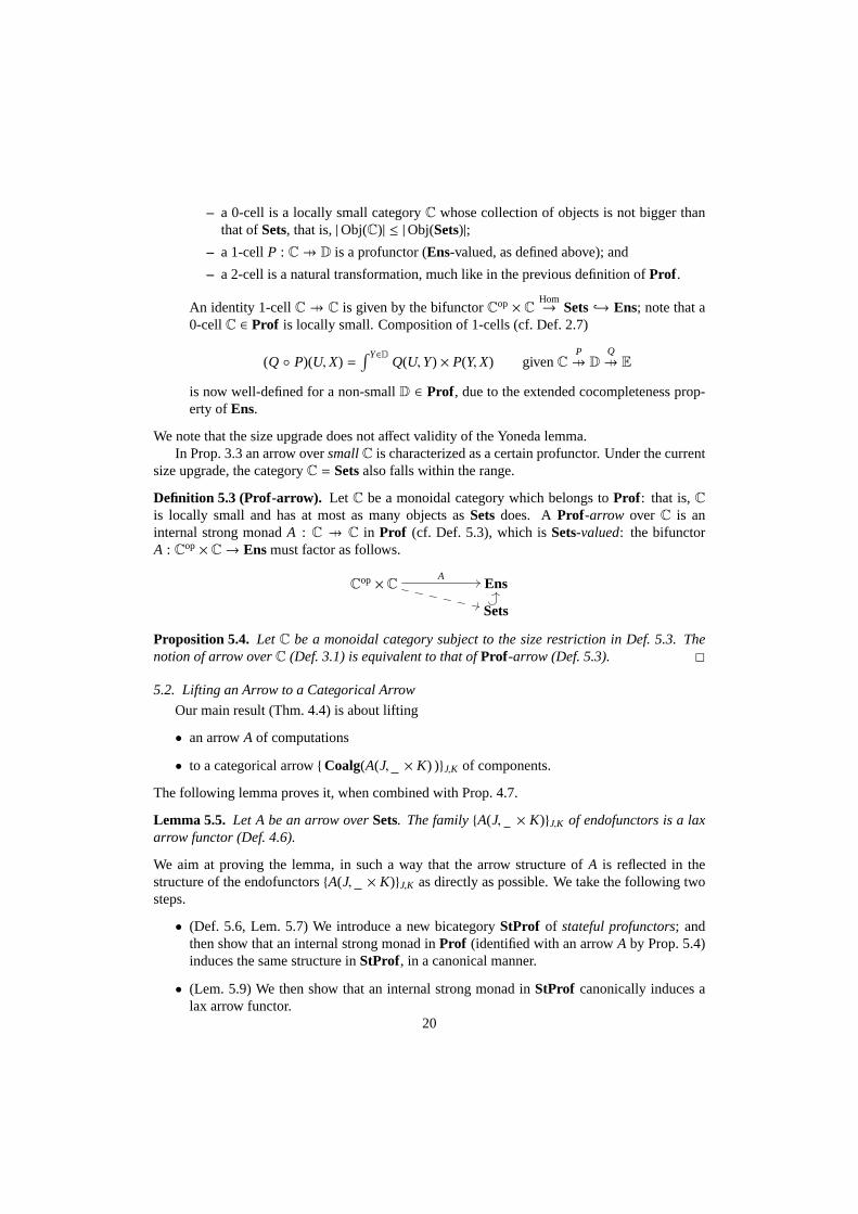
Definition 5.3 (Prof-arrow). Let C be a monoidal category which belongs toProf : that is,Cis locally small and has at most as many objects asSetsdoes. AProf -arrow over C is aninternal strong monadA : C p→ C in Prof (cf. Def. 5.3), which isSets-valued: the bifunctorA : C

op × C→ Ens must factor as follows.

Cop × CA

Ens

Sets

Proposition 5.4. Let C be a monoidal category subject to the size restriction in Def. 5.3. Thenotion of arrow overC (Def. 3.1) is equivalent to that ofProf -arrow (Def. 5.3). 2

5.2. Lifting an Arrow to a Categorical Arrow

Our main result (Thm. 4.4) is about lifting

• an arrowA of computations

• to a categorical arrow{Coalg(A(J, × K) )}J,K of components.

The following lemma proves it, when combined with Prop. 4.7.

Lemma 5.5. Let A be an arrow overSets. The family{A(J, × K)}J,K of endofunctors is a laxarrow functor (Def. 4.6).

We aim at proving the lemma, in such a way that the arrow structure of A is reflected in thestructure of the endofunctors{A(J, × K)}J,K as directly as possible. We take the following twosteps.

• (Def. 5.6, Lem. 5.7) We introduce a new bicategoryStProf of stateful profunctors; andthen show that an internal strong monad inProf (identified with an arrowA by Prop. 5.4)induces the same structure inStProf, in a canonical manner.

• (Lem. 5.9) We then show that an internal strong monad inStProf canonically induces alax arrow functor.

20

This separation of steps offers a more structured view of the calculations in the earlierversion [1]of the paper. For instance, the equalities in [1, Table 3] cannow be systematically understoodas the axioms for an internal strong monad inStProf, translated into 2-cells inProf . For therecord we shall present as many technical details as the space allows. The details may seemoverwhelming; nevertheless, as is often the case with 2-categorical/bicategorical arguments, theunderlying intuition is simple.

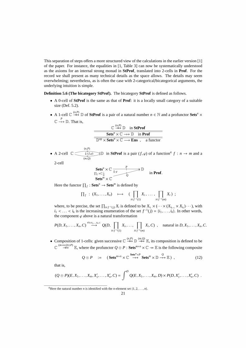
Definition 5.6 (The bicategory StProf). The bicategoryStProf is defined as follows.

• A 0-cell of StProf is the same as that ofProf : it is a locally small category of a suitablesize (Def. 5.2).

• A 1-cell C(n,P)◦−→ D of StProf is a pair of a natural numbern ∈ N and a profunctorSetsn ×

CPp−→ D. That is,

C(n,P)◦−→ D in StProf

Setsn × C p−→ D in ProfDop × Setsn × C −→ Ens , a functor

• A 2-cell C◦

(n,P)

◦(m,Q)

⇓ ( f ,ϕ) D in StProf is a pair (f , ϕ) of a function4 f : n → m and a

2-cell

Setsn × CP

⇓ ϕ∏

f ×C

D

Setsm × C

Qin Prof .

Here the functor∏

f : Setsn→ Setsm is defined by

∏

f : (X1, . . . ,Xn) 7−→(

∏

i∈ f −1(1)

Xi , . . . ,∏

i∈ f −1(m)

Xi)

;

where, to be precise, the set∏

i∈ f −1( j) Xi is defined to beXi1 × (· · · × (Xik−1 × Xik) · · · ), withi1 < . . . < ik is the increasing enumeration of the setf −1( j) = {i1, . . . , ik}. In other words,the componentϕ above is a natural transformation

P(D,X1, . . . ,Xn,C)ϕD,X1,...,Xn,C

−→ Q(D,∏

i∈ f −1(1)

Xi , . . . ,∏

i∈ f −1(m)

Xi ,C) , natural inD,X1, . . . ,Xn,C.

• Composition of 1-cells: given successiveC(n,P)◦−→ D

(m,Q)◦−→ E, its composition is defined to be

C(m+n,Q⊚P)◦−→ E, where the profunctorQ ⊚ P : Setsm+n ×C p→ E is the following composite

Q ⊚ P :=(

Setsm+n × CSetsm×P

p−→ Setsm × DQp−→ E)

, (12)

that is,

(Q ⊚ P)(E,X1, . . . ,Xm,X′1, . . . ,X

′n,C) =

∫ D

Q(E,X1, . . . ,Xm,D) × P(D,X′1, . . . ,X′n,C) .

4Here the natural numbern is identified with then-element set{1,2, . . . ,n}.

21

• Identity 1-cells: givenC ∈ StProf, the identity 1-cell onC is defined to be (0,Hom) :C ◦−→ C, using the hom-functor.

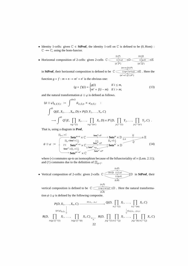
• Horizontal composition of 2-cells: given 2-cellsC◦

(n,P)

◦(n′,P′)

⇓ ( f ,ϕ) D◦

(m,Q)

◦(m′,Q′)

⇓ (g,ψ) E

in StProf, their horizontal composition is defined to beC◦

(m+n,Q⊚P)

◦(m′+n′,Q′⊚P′)

⇓ (g+ f ,ψ⊚ϕ) E . Here the

functiong+ f : m+ n→ m′ + n′ is the obvious one:

(g+ f )(i) =

g(i) if i ≤ m,

m′ + f (i −m) if i > m;(13)

and the natural transformationψ⊚ ϕ is defined as follows.

(ψ⊚ ϕ)E,~X,~Y,C :=∫ D∈D

ψE,~X,D × ϕD,~Y,C :

∫ D

Q(E,X1, . . . ,Xm,D) × P(D,Y1, . . . ,Yn,C)

−→

∫ D

Q′(E,∏

i∈g−1(1)

Xi , . . . ,∏

i∈g−1(m′)

Xi ,D) × P′(D,∏

j∈ f −1(1)

Yj , . . . ,∏

j∈ f −1(n′)

Yj ,C) .

That is, using a diagram inProf ,

ψ⊚ ϕ :=

Setsm+n × CSetsm×P

∏

g ×Setsn×C

∏

g+ f ×C

(†)

(∗)

Setsm × DQ

⇓ ψ∏

g ×D

E

Setsm′+n × C

Setsm′×P

⇓ Setsm′×ϕ

Setsm′×∏

f ×C

Setsm′

× D

Q′

Setsm′+n′ × C

Setsm′×P′

(14)

where (∗) commutes up-to an isomorphism because of the bifunctoriality of × (Lem. 2.11);and (†) commutes due to the definition of

∏

g+ f .

• Vertical composition of 2-cells: given 2-cellsC◦

(n,P)

◦(m,Q) ⇓ ( f ,ϕ)

⇓ (g,ψ)◦

(k,R)

D in StProf, their

vertical composition is defined to beC◦

(n,P)

◦(k,R)

⇓ (g◦ f ,ψ⊙ϕ) D . Here the natural transforma-

tion ψ ⊙ ϕ is defined by the following composite.

P(D,X1, . . . ,Xn,C)

(ψ⊙ϕ)D,~X,C

ϕD,X1,...,Xn,C Q(D,∏

i∈ f −1(1)

Xi , . . . ,∏

i∈ f −1(m)

Xi ,C)

ψD,∏

Xi ,...,∏

Xi ,C

R(D,∏

i∈(g◦ f )−1(1)

Xi , . . . ,∏

i∈(g◦ f )−1(k)

Xi ,C) R(D,∏

j∈g−1(1)

∏

i∈ f −1( j)

Xi , . . . ,∏

j∈g−1(k)

∏

i∈ f −1( j)

Xi ,C)�

22

The isomorphism on the bottom row arises from the canonical isomorphisms∏

j∈g−1(1)

∏

i∈ f −1( j)

Xi�

−→∏

i∈(g◦ f )−1(1)

Xi , . . . ,∏

j∈g−1(k)

∏

i∈ f −1( j)

Xi�

−→∏

i∈(g◦ f )−1(k)

Xi (15)

in a symmetric monoidal category (Sets,×,1); note that we have (g ◦ f )−1(l) =∐

j∈g−1(l)

f −1( j).

Using a diagram inProf , the above definition amounts to

ψ ⊙ ϕ :=

Setsn × C P∏

f ×C

∏

g◦ f ×C

�⇐β

Setsm × CQ

⇓ ψ

⇓ ϕ

∏

g ×C

D

Setsk × C R

, (16)

where the isomorphismβ is the canonical ones like in (15), bundled up together. We shallrefer to suchβ as anormalizing isomorphism.

It is straightforward to verify that the above data togetherform a bicategory.

As we did forProf (see (9)), we also extend the operation× of taking product categories to a

“tensor” inStProf. GivenC(n,F)◦−→ D andC

′(n′,F′)◦−→ D

′, we define the 1-cellC×C′

(n,F)×(n′,F′)◦−→ D×D

′

to be the pair (n+ n′, F × F′) : C×C′ ◦−→ D×D

′, whereF × F′ is the profunctor defined in (9).

Lemma 5.7. Let A be an arrow overSets. The 1-cell

(1,A) : Sets ◦−→ Sets in StProf,

where a profunctorA is defined by

A : Setsop × Sets× Sets−→ Sets −→ Ens , (J,X,K) 7−→ A(J,X × K) ,

is canonically an internal strong monad inStProf.

Notations 5.8. In what follows we often denote the categorySetsby S, for the sole purpose ofsaving space. The operation× : Sets× Sets→ Setsof taking products of sets is often denotedby ⊠ instead, to distinguish it from product of categories and the “tensors” onProf andStProf.

Recall that we denote a functorF : C → D, embedded inProf by taking its direct imageF∗, also byF (Notations 2.10). We shall extend this convention toStProf. Namely, given afunctor F : C → D, we denote its embedding (0, F∗) : C ◦→ D also byF. Recall also that weoften denote the identity 1-cell idC : C p→ C in Prof by C (Notations 2.10); we shall use thisconvention forStProf, too.

Proof. (Of Lem. 5.7) What we need to do is

• to equip the 1-cell (1,A) with the following “operator” 2-cells, all of them inStProf:

S◦

S= (0,Hom)

◦

(1,A)

⇓ arr S ,S ◦

(1,A)

◦

(1,A)

⇓>>>

S ◦(1,A)

S,

S2 ◦(1,A)×S= (1,A×S)

◦⊠= (0,⊠) ⇓ first

S2

◦ (0,⊠)

S ◦

(1,A)S

;

23

• and to prove that these 2-cells satisfy the same equational axioms as in Table 1.

A 2-cell of the type ofarr above is the same thing as a 2-cell

1× S1×S

S

⇓S

S× S A=A(−,+1⊠+2), hence

1× S1×S

π2

⇓

S

S× S⊠

SA ;

here we used the equality

A =(

S2⊠

p−→ SAp−→ S)

(17)

that follows from the Yoneda lemma (Lem. 2.5).We construct a 2-cell of the last type as follows, usingA’s arrow structure (specifically itsarr

operator). The iso 2-cellλ therein is the left unitalityλX : 1 ⊠ X �→ X, embedded inProf .

arr :=S

〈1,S〉

S

� ⇓ λ−1

S

S2⊠

SS ⇒

arr A (18)

Similarly, a 2-cell of the type of>>> is identified with S2 × S⊠×S

A⊚A

⇓S

S× S A

; using the defini-

tion (12) of⊚ and also (17), this is further identified with the 2-cellS3

⊠×S

S×⊠

⇓

S2 S×AS2 ⊠

SA

S

S2⊠

SA

in Prof . Such a 2-cell can be constructed as follows.

>>> :=S3

⊠×S

S×⊠

� ⇓α−1

S2 S×A

⊠

S2 ⊠

⇓ secondS

A

S2⊠

SA

A

⇓>>>

S(19)

Hereα is the associativity isomorphism (X⊠Y)⊠Z �→ X⊠ (Y⊠Z); second is a derived operatorof the arrowA (Def. 3.5); and>>> is an arrow operator ofA.

A 2-cell of the type offirst is identified with S× S2

S×S2

⊠⊚(A×S)

⇓S× S2

S× S A⊚⊠

in Prof , by the defi-

nition of StProf. Again expanding⊚ and A using (12) and (17), it is identified with a 2-cell

S3 ⊠×S

S×⊠S2 A×S

⇓

S2

⊠

S2⊠

SA

Sin Prof . We define

first :=S3 ⊠×S

S×⊠ � ⇓α

S2 A×S

⊠ ⇓ firstS2

⊠

S2⊠

SA

S. (20)

24

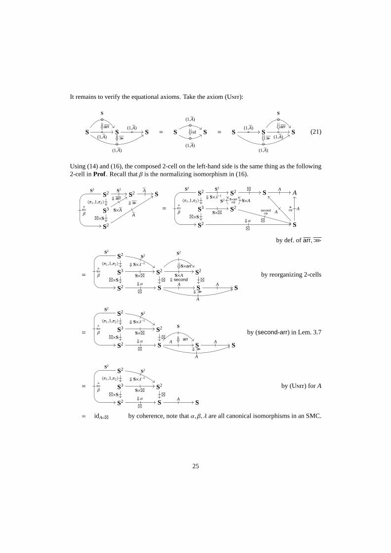
It remains to verify the equational axioms. Take the axiom (Unit):

S

◦S

arr◦

(1,A)

◦(1,A)

>>>S ◦

(1,A)S = S

◦(1,A)

◦(1,A)

id S = S ◦(1,A)

◦(1,A)

>>>S

◦S

arr◦

(1,A)S (21)

Using (14) and (16), the composed 2-cell on the left-hand side is the same thing as the following2-cell inProf . Recall thatβ is the normalizing isomorphism in (16).

S2

〈π1,1,π2〉

S2

⇓ arr

S2

�

⇐β

S2 AS

S3 S×A

⊠×S

S2

A

⇓>>>

=

S2

〈π1,1,π2〉

S2

⇓ S×λ−1

S2

�

⇐β

S2 ⊠S

AA

S3S×⊠

⊠×S

S2

S2 S×AS×arr⇒

⊠

second⇒

S2⊠

⇓αS

AA>>>

⇒

by def. ofarr, >>>

=

S2

〈π1,1,π2〉

S2

⇓ S×λ−1

S2

�

⇐β S3

S×⊠⊠×S

S2

⇓ second

S2

S×arr

S×A⊠

S2

⊠

S2⊠

⇓αS

A

A

⇓ >>>S

AS

by reorganizing 2-cells

=

S2

〈π1,1,π2〉

S2

⇓ S×λ−1

S2

�

⇐β S3

S×⊠⊠×S

S2

⊠

S2⊠

⇓αS

A

A

⇓ >>>

S

arr

SA

S

by (second-arr) in Lem. 3.7

=

S2

〈π1,1,π2〉

S2

⇓ S×λ−1

S2

�

⇐β S3

S×⊠⊠×S

S2

⊠

S2⊠

⇓αS

AS

by (Unit) for A

= idA◦⊠ by coherence, note thatα, β, λ are all canonical isomorphisms in an SMC.

25

Similarly, the composed 2-cell on the right-hand side of (21) is the following 2-cell inProf .

S2

〈1,π1,π2〉

AS2

�

⇐β

SS

⇓ arr〈1,S〉

S

S3S×A

⊠×S

S2 A

S2A

⇓>>>

=

S2

〈1,π1,π2〉

⊠S2

�

⇐β

SA

SS

⇓ λ−1

〈1,S〉

S3S×⊠

⊠×S ⇓ α−1

S2S×A

⊠ ⇓ second

S2

⊠

S2⊠

SA

A

⇓ >>>S

A

S

⇓ arr S

by def. ofarr, >>>

=

S2

〈1,π1,π2〉

⊠S2

�

⇐β

SA

SS

�

⇐λ−1

〈1,S〉

S3S×⊠

⊠×S ⇓ α−1

S2S×A

⊠ ⇓ second

S2

⊠

S2⊠

SA

S

by (Unit) for A

=

S2

〈1,π1,π2〉

⊠S2

�

⇐β

S〈1,S〉

S�

⇐λ−1S3

S×⊠⊠×S ⇓ α−1

S2

⊠

S2⊠

SA

S

by (second-λ) in Lem. 3.7

= idA◦⊠ by coherence for (S,⊠,1).

Similar straightforward calculations verify the other axioms for (1,A) in StProf. In its coursewe use (14), (16), the axioms forA (Table 1) and the equalities in Table 2. We present the proofsfor the axioms (Assoc) and (first->>>). Recall that 1-cells denoted by◦→ means the diagram is inStProf; 1-cells denoted byp→ means it is inProf .

For the axiom (Assoc),

S ◦(1,A)

◦

(1,A)

⇓>>>

S ◦(1,A)

◦(1,A)

>>>S ◦

(1,A)S

=

S4

⊠×S2

S2×⊠(⊠×S)◦(S×⊠×S)

�

⇐β

S3

⊠×S

S2×AS3

⊠×S

S×⊠

⇓ α−1

S2

⊠

S×A

⇓ second

S2

⊠

S3S×⊠

⊠×S ⇓ α−1

S2S×A

⊠

S2⊠

SA

A

⇓ >>>S

AS

S2⊠

SA⇓ second

A

⇓ >>>

26

=

S4 S2×⊠

S×⊠×S ⇓ S×α−1

S3 S2×A

S×⊠⊠×S

S3⊠×S

S×⊠

S3S×⊠

⊠×S ⇓ α−1

S2

⊠

α⇐ S2

S×A

⊠⇓ second

S2

⊠

α−1⇐S2

⊠S×A

⇓ second

S2

⊠

S2⊠

SA

A

⇓ >>>

SA

A

⇓ >>>S

AS

by coherence for (S,⊠,1)

=

S4 S2×⊠

S×⊠×S ⇓ S×α−1

S3 S2×A

S×⊠ ⇓ S×second

S3

S×⊠

S3S×⊠

⊠×S ⇓ α−1

S2S×A

⊠ ⇓ second

S2

⊠S×A

⇓ second

S2

⊠

S2⊠

SA

A

⇓ >>>

SA

A

⇓ >>>S

AS

by (second-α)

=

S4 S2×⊠

S×⊠×S ⇓ S×α−1

S3 S2×A

S×⊠ ⇓ S×second

S3

S×⊠

S3S×⊠

⊠×S ⇓ α−1

S2S×A

⊠ ⇓ second

S2

⊠S×A

⇓ second

S2

⊠

S2⊠

SA

A

⇓ >>>A

⇓ >>>S

AS

AS

by (Assoc)

=

S4 S2×⊠

S×⊠×S ⇓ S×α−1

S3 S2×A

S×⊠ ⇓ S×second

S3

S×⊠

S3S×⊠

⊠×S ⇓ α−1

S2S×A

⊠S×A

⇓ S×>>>S2

S×A S2

⊠

S2⊠

S

A

⇓ >>>A

⇓ secondS

AS

by (second->>>)

=

S ◦(1,A)

◦

(1,A)

⇓>>>

◦(1,A)

>>>S ◦

(1,A)S ◦

(1,A)S

.

27

For the axiom (first->>>),

S2 ◦(1,A)×S

⇓ first◦⊠

S2 ◦(1,A)×S

⇓ first◦⊠

S2

◦⊠

S ◦(1,A)

(1,A)

>>>S ◦

(1,A)S

=

S4 S×⊠×S

S2×⊠ ⇓ S×αS3

S×⊠

S×A×S

⇓ S×first

S3

S×⊠

⊠×S

⇓ α

S2

⊠

A×S

⇓ first

S2

⊠

S3S×⊠

⊠×S⇓ α−1

S2S×A

⊠

S2⊠

⇓ second

SA

S

S2⊠

SA

A

⇓ >>>

=

S4 S×⊠×S

S2×⊠

S3

⊠×S

S×A×S

⇓ second×SS3

⊠×S

S3

⊠×S

�

⇐ S2A×S

⊠ ⇓ first

S2A×S

⊠ ⇓ first

S2

⊠

S2⊠

SA

A

⇓ >>>S

AS

by (first-second) in Lem. 3.7

=

S4 S×⊠×S

S2×⊠

S3

⊠×S

S×A×S

⇓ second×SS3

⊠×S

S3

⊠×S

�

⇐ S2A×S

⊠A×S

⇓ >>>×CS2

A×S S2

⊠

S2⊠

S

A

⇓ firstS

by (first->>>)

=

S2 ◦(1,A)×S

(1,A)×S

>>>×S

◦⊠

S2 ◦(1,A)×S

S2

◦⊠

S ◦

(1,A)

⇓ first

S

.

This concludes the proof. 2

Lemma 5.9. Let S(1,P)◦−→ S be an internal strong monad inStProf, equipped with “operator”

2-cellsarr, >>> andfirst. Assume that P isSets-valued: that is,

for each J,X,K ∈ Sets, the collection P(J,X,K) ∈ Ens is small and hence belongsto the categorySets.

Then the family{FJ,K}J,K∈Setsof functors, defined by

FJ,K := P(J, ,K) : Sets−→ Sets

is canonically a lax arrow functor (Def. 4.6).28

Proof. What we have to do is to define three “operators”Farr f , F>>> andFfirst and show that theysatisfy the equalities in Table 3.

Given a functionf : J → K in Sets, to defineFarr f : 1 −→ FJ,K1 = P(J,1,K) we use

the “operator” S◦

(0,S)

◦(1,P)

arr S . By Def. 5.6, the latter 2-cell inStProf is identified with a natural

transformationarrJ,K : S(J,K) −→ P(J,1,K), natural inJ,K. We set

Farr f := (arrJ,K)( f ) . (22)

Similarly by Def. 5.6, the operator>>> is identified with a natural transformation

>>>J,X,Y,L :∫ K∈S

P(J,X,K) × P(K,Y, L) −→ P(J,X × Y, L) , natural inJ,X,Y, L.

We set (F>>>J,K,L )X,Y to be the composite

(F>>>J,K,L )X,Y :=(

P(J,X,K)×P(K,Y, L)ιK−→

∫ K∈S

P(J,X,K)×P(K,Y, L)>>>J,X,Y,L−→ P(J,X×Y, L)

)

.

(23)HereιK denotes a coprojection into a coend.

To defineFfirst, note the following bijective correspondence

ΦJ,X,K,L,Y,M :[

P(J,X,K),P(L,Y,M)] �

−→ Nat(

[ , L] × P(J,X,K) , P( ,Y,M))

; (24)

where [−,+] denotes the function space, i.e. the hom-set functor forS. We denote the correspon-dence byΦ. The correspondence is derived from the Yoneda lemma (Lem. 2.4, see also Cor. 2.3)as well as from the adjunctionS × ⊣ [S, ]; due to the naturality of the both ingredients, thecorrespondenceΦ in (24) is obviously natural inJ,X,K, L,Y,M.

By Def. 5.6, the operatorS2 ◦

(1,P)×S= (1,P×S)

◦⊠= (0,⊠) ⇓ first

S2

◦ (0,⊠)

S ◦(1,P)

Sis a natural transformation

firstU,X,K,L :∫ J,V∈S

[U, J × V] × P(J,X,K) × [V, L] −→∫ W∈S

P(U,X,W) × [W,K × L] ;

using this and (24), we defineFfirst as follows.

(FfirstJ,K,L )X := Φ−1J,X,K,J×L,X,K×L

[ , J × L] × P(J,X,K)�

Yoneda

∫ V[ , J × V] × P(J,X,K) × [V, L]

ιJ ∫ J,V[ , J × V] × P(J,X,K) × [V, L]

first ,X,K,L ∫ WP( ,X,W) × [W,K × L]

�

YonedaP( ,X,K × L)

. (25)

29

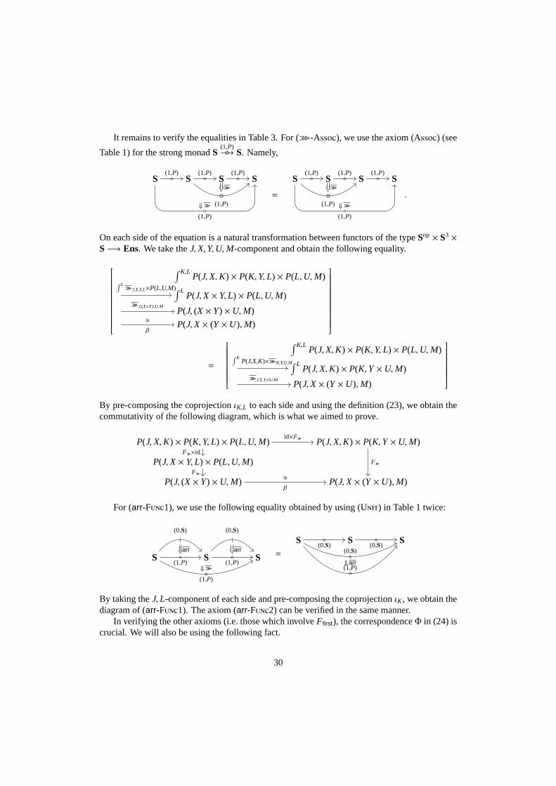
It remains to verify the equalities in Table 3. For (>>>-Assoc), we use the axiom (Assoc) (see

Table 1) for the strong monadS(1,P)◦−→ S. Namely,

S ◦(1,P)

◦(1,P)

⇓>>>

S ◦(1,P)

◦(1,P)

>>>S ◦

(1,P)S

=

S ◦(1,P)

◦(1,P)

⇓>>>

◦(1,P)

>>>S ◦

(1,P)S ◦

(1,P)S

.

On each side of the equation is a natural transformation between functors of the typeSop × S3 ×

S−→ Ens. We take theJ,X,Y,U,M-component and obtain the following equality.

∫ K,LP(J,X,K) × P(K,Y, L) × P(L,U,M)

∫ L>>>J,X,Y,L×P(L,U,M)∫ L

P(J,X × Y, L) × P(L,U,M)>>>J,(X×Y),U,M

P(J, (X × Y) × U,M)�

βP(J,X × (Y× U),M)

=

∫ K,LP(J,X,K) × P(K,Y, L) × P(L,U,M)

∫ KP(J,X,K)×>>>K,Y,U,M∫ L

P(J,X,K) × P(K,Y× U,M)>>>J,X,Y×U,M

P(J,X × (Y× U),M)

By pre-composing the coprojectionιK,L to each side and using the definition (23), we obtain thecommutativity of the following diagram, which is what we aimed to prove.

P(J,X,K) × P(K,Y, L) × P(L,U,M)id×F>>>

F>>>×id

P(J,X,K) × P(K,Y× U,M)

F>>>P(J,X × Y, L) × P(L,U,M)F>>>

P(J, (X × Y) × U,M) �

βP(J,X × (Y× U),M)

For (arr-Func1), we use the following equality obtained by using (Unit) in Table 1 twice:

S ◦(1,P)

◦(1,P)

⇓>>>

(0,S)

arrS ◦

(1,P)

(0,S)

arrS =

S ◦(0,S)

◦(0,S)

⇓ arr

◦(1,P)

S ◦(0,S)

S

By taking theJ, L-component of each side and pre-composing the coprojectionιK , we obtain thediagram of (arr-Func1). The axiom (arr-Func2) can be verified in the same manner.

In verifying the other axioms (i.e. those which involveFfirst), the correspondenceΦ in (24) iscrucial. We will also be using the following fact.

30

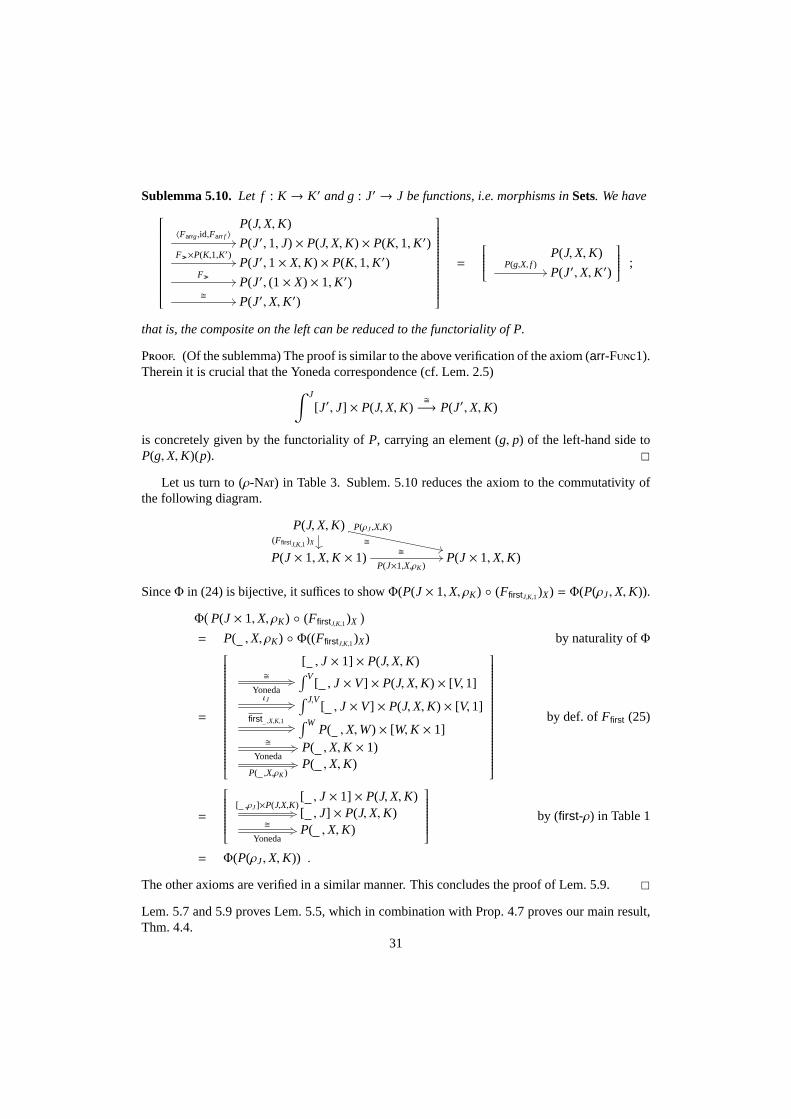
Sublemma 5.10.Let f : K → K′ and g: J′ → J be functions, i.e. morphisms inSets. We have

P(J,X,K)〈Farrg,id,Farr f 〉

P(J′,1, J) × P(J,X,K) × P(K,1,K′)F>>>×P(K,1,K′)

P(J′,1× X,K) × P(K,1,K′)F>>>

P(J′, (1× X) × 1,K′)�

P(J′,X,K′)

=

P(J,X,K)P(g,X, f )

P(J′,X,K′)

;

that is, the composite on the left can be reduced to the functoriality of P.

Proof. (Of the sublemma) The proof is similar to the above verification of the axiom (arr-Func1).Therein it is crucial that the Yoneda correspondence (cf. Lem. 2.5)

∫ J

[J′, J] × P(J,X,K)�

−→ P(J′,X,K)

is concretely given by the functoriality ofP, carrying an element (g, p) of the left-hand side toP(g,X,K)(p). 2

Let us turn to (ρ-Nat) in Table 3. Sublem. 5.10 reduces the axiom to the commutativity ofthe following diagram.

P(J,X,K)�

P(ρJ,X,K)

(FfirstJ,K,1 )X

P(J × 1,X,K × 1) �

P(J×1,X,ρK )P(J × 1,X,K)

SinceΦ in (24) is bijective, it suffices to showΦ(P(J × 1,X, ρK) ◦ (FfirstJ,K,1)X) = Φ(P(ρJ,X,K)).

Φ(

P(J × 1,X, ρK) ◦ (FfirstJ,K,1)X)

= P( ,X, ρK) ◦ Φ((FfirstJ,K,1)X) by naturality ofΦ

=

[ , J × 1] × P(J,X,K)�

Yoneda

∫ V[ , J × V] × P(J,X,K) × [V,1]

ιJ ∫ J,V[ , J × V] × P(J,X,K) × [V,1]

first ,X,K,1 ∫ WP( ,X,W) × [W,K × 1]

�

YonedaP( ,X,K × 1)

P( ,X,ρK )P( ,X,K)

by def. ofFfirst (25)

=

[ , J × 1] × P(J,X,K)[ ,ρJ]×P(J,X,K)

[ , J] × P(J,X,K)�

YonedaP( ,X,K)

by (first-ρ) in Table 1

= Φ(P(ρJ,X,K)) .

The other axioms are verified in a similar manner. This concludes the proof of Lem. 5.9. 2

Lem. 5.7 and 5.9 proves Lem. 5.5, which in combination with Prop. 4.7 proves our main result,Thm. 4.4.

31

6. Conclusions and Future Work

Inspired by the common graphical understanding (boxes connected by typed wires), we haveelaborated on a connection between computations and components; more specifically, algebraicstructure possessed by these. The algebraic structure of computations has been axiomatized bythe notion of arrow—by Hughes [4]—which is equivalent to that of Freyd category [5, 6]. Wehave demonstrated that the arrow structure is also carried by components. Its operators (arr, >>>andfirst) serve asconnectorsbetween components, hence as a basiccomponent calculus. Thelatter “component-arrow” turns out to be acategorified[12] notion of arrow, whose satisfactionof axioms only up-to isomorphisms is exemplary.

Our technical contribution is as follows. Arrow-basedA-components—described as coal-gebras, withA representing the machines’ computation effect—carry canonical (categorified)arrow structure, which is in fact a lifting of the arrow structure of A itself. The “lifting” is bestpresented inProf , the bicategory of categories and profunctors. There we rely on the secondauthor’s observation [16] that an arrowA is the same thing as an internal strong monad inProf .When compared to the previous workshop version [1], the current version presents the liftingprocess in a more structural manner, using a novel bicategory StProf.

The notion of categorical arrow, as a component calculus, isvery basic. In fact for the notionof arrow (composing computations) some extensions have been proposed. Notable among themis an extension with a feedback/loop operator [28, 29]. Its categorified version—that is, thecorresponding (extended) component calculus—has been studied in [24]. However, unlike thecurrent work, the calculations in [24] are all direct and do not happen inProf . Much like thecharacterization in [16], the current authors have formulated an arrow with loop as a monad inProf with suitable additional structure. Unfortunately we havenot yet found its good use.

Acknowledgments.Thanks are due to Paul-Andre Mellies for advocating use of profunctors; toMarcelo Fiore, Bart Jacobs, Bartek Klin and Paul Blain Levy for helpful discussions; and to thereviewers of the earlier version [1] for useful comments.

[1] K. Asada, I. Hasuo, Categorifying computations into components via arrows as profunctors, in: CoalgebraicMethods in Computer Science (CMCS 2010), Elect. Notes in Theor. Comp. Sci. To appear.

[2] E. Moggi, Notions of computation and monads, Inf. & Comp. 93(1) (1991) 55–92.[3] T. Uustalu, V. Vene, Comonadic notions of computation, Elect. Notes in Theor. Comp. Sci. 203 (2008) 263–284.[4] J. Hughes, Generalising monads to arrows., Science of Comput. Progr. 37 (2000) 67–111.[5] J. Power, E. Robinson, Premonoidal categories and notions of computation., Math. Struct. in Comp. Sci. 7 (1997)

453–468.[6] P. B. Levy, A. J. Power, H. Thielecke, Modelling environments in call-by-value programming languages, Inf. &

Comp. 185 (2003) 182–210.[7] B. Jacobs, C. Heunen, I. Hasuo, Categorical semantics forarrows, J. Funct. Progr. 19 (2009) 403–438.[8] R. Atkey, What is a categorical model of arrows?, in: V. Capretta, C. McBride (Eds.), Mathematically Structured

Functional Programming.[9] L. Barbosa, Components as Coalgebras, Ph.D. thesis, Univ. Minho, 2001.

[10] I. Hasuo, C. Heunen, B. Jacobs, A. Sokolova, Coalgebraic components in a many-sorted microcosm, in: A. Kurz,M. Lenisa, A. Tarlecki (Eds.), CALCO, volume 5728 ofLect. Notes Comp. Sci., Springer, 2009, pp. 64–80.

[11] J. J. M. M. Rutten, Universal coalgebra: a theory of systems, Theor. Comp. Sci. 249 (2000) 3–80.[12] J. C. Baez, J. Dolan, Categorification, Contemp. Math. 230 (1998) 1–36.[13] J. C. Baez, J. Dolan, Higher dimensional algebra III:n-categories and the algebra of opetopes, Adv. Math 135

(1998) 145–206.[14] I. Hasuo, B. Jacobs, A. Sokolova, The microcosm principle and concurrency in coalgebra, in: Foundations of

Software Science and Computation Structures, volume 4962 ofLect. Notes Comp. Sci., Springer-Verlag, 2008, pp.246–260.

[15] R. Street, The formal theory of monads, Journ. of Pure & Appl. Algebra 2 (1972) 149–169.

32

[16] K. Asada, Arrows are strong monads, in: Mathematically Structured Functional Programming (MSFP 2010). Toappear.

[17] G. M. Kelly, Basic Concepts of Enriched Category Theory, number 64 in LMS, Cambridge Univ. Press, 1982.Available online:http://www.tac.mta.ca/tac/reprints/articles/10/tr10abs.html.

[18] S. Mac Lane, Categories for the Working Mathematician, Springer, Berlin, 2nd edition, 1998.[19] M. Barr, C. Wells, Toposes, Triples and Theories, Springer, Berlin, 1985. Available online.[20] J. Benabou, Distributors at work, Lecture notes taken by T. Streicher, 2000.

www.mathematik.tu-darmstadt.de/∼streicher/FIBR/DiWo.pdf.gz.[21] F. Borceux, Handbook of Categorical Algebra, volume 50,51 and 52 ofEncyclopedia of Mathematics, Cambridge

Univ. Press, 1994.[22] M. Fiore, Rough notes on presheaves, 2001. Available online.[23] A. Kock, Monads on symmetric monoidal closed categories, Arch. Math. XXI (1970) 1–10.[24] I. Hasuo, B. Jacobs, Component traces, 2010. Preprint.[25] S. Abramsky, E. Haghverdi, P. Scott, Geometry of interaction and linear combinatory algebras, Math. Struct. in

Comp. Sci. 12 (2002) 625–665.[26] A. Joyal, R. Street, D. Verity, Traced monoidal categories, Math. Proc. Cambridge Phil. Soc. 119(3) (1996)

425–446.[27] J. M. E. Hyland, A small complete category, Ann. Pure & Appl. Logic 40 (1988) 135–165.[28] N. Benton, M. Hyland, Traced premonoidal categories, Theoretical Informatics and Applications 37 (2003) 273–

299.[29] R. Paterson, A new notation for arrows, in: ICFP, pp. 229–240.

33