cash flow analysis by the prudent banker's of society of actuaries 1987 vol. 39 cash flow...

TRANSACTIONS OF SOCIETY OF ACTUARIES 1987 VOL. 39

CASH FLOW ANALYSIS BY THE PRUDENT BANKER'S METHOD, OR DISCOUNTING TURNED ON ITS HEAD

CLAUDE Y. PAQUIN

ABSTRACT

Prudent bankers charge more on loans than they pay on deposits. In the cycle of life insurance products, it often happens that the insurer's cash flow alternates between positive and negative. Figures concerning corporate return on equity (ROE) are nothing short of delusive unless one knows whose equity, the stockholders' (as lenders or investors), or the policyholders' (as depositors), is involved at every step of a series of transactions creating cash flows. Traditional discounting is hazardous to corporate health unless, as this paper demonstrates, it is turned on its head and insurance managers adopt the methods of prudent bankers.

INTRODUCTION

Ever since Anderson's seminal paper on the calculation of gross premiums and profit measurement for nonpar insurance was published in 1959 (TSA XI, 357), actuaries have encountered special situations where it seemed that the methods suggested in that paper did not work well. The paper's basic premise was that the insurer (or its stockholders) would invest funds toward the production of a block of life insurance policies and that the insurer would later gradually recover these funds out of the profits generated by that block of business. What if later policy years produced losses rather than profits, as is often the case with limited-payment decreasing term insurance? What if there was no first-year "investment in the business," in products with relatively low first-year commissions and other expenses (as with some mail- order products, for instance)? What if the income tax consequences of selling at an apparent loss reduced the effective first-year "investment in the business" to a much lower, and perhaps inconsequential or even negative, amount?

These questions appeared never to have been answered satisfactorily in the actuarial literature, although it has been suggested that gross premiums should incorporate, in their computation, separate risk and service charges, so that policyholders may reward the insurer's investors for something when a product sale occasions no measurable investment in the business by the insurer.* *Paquin, C.Y. "Current Concepts of Product Development," Best's Review, Life/Health Insurance

Edition, October 1969. Paquin, C.Y. "A Step by Step Approach to Calculating Gross Premiums," ARCH, June 1978.

177

178 CASH FLOW ANALYSIS

As every actuarial student knows, the rate of return on equity (ROE), or rate of return on investment (ROI), is that interest rate which, when used to compute the present (or discounted) value of future profits makes that value equal to the initial investment. In the boardroom, that's how it is presented, and that's how it is understood. Everyone understands it.

Everyone understands except the actuary who runs into insurance products with no first-year investment (by the insurer), or with annual losses to the insurer interspersed in a string of annual profits, or with a benefit tail pre- funded by previous premium receipts (such as in limited-payment decreasing term).

To further compound the actuary's problem, he can see clearly that some insurer equity is truly at risk, as where the cash flow is actually negative, while he realizes also that some insurer equity is merely immobilized through legally required reserves. (Sometimes these statutory reserves exceed the absolute legal minimum.) Where an insurer must freeze stockholder equity into a legally required reserve, one might more properly speak of "equity at work" than of "equity at risk." And one should perhaps consider a lesser reward, or lesser return objective, for equity at work than for equity truly at risk. But that is a somewhat different matter, to be considered later.

THE PRUDENT B A N K E R ' S APPROACH

Prudent bankers charge more on loans than they pay on deposits. One might say that it's out of presumptuousness: the banker presumes

that when he lends money he runs a risk of not getting it back, for which he should be compensated, while when the public lends him money, through deposits (evidenced by certificates of deposit, passbooks or otherwise), the public runs no risk. (Contemporary events suggest this is not always true. But that's the reasoning.)

One might say that it's out of enlightened self-interest, for simple economic survival in the free enterprise system, i.e., to cover his costs and obtain a reward for the services he provides. This point need not be labored. Suffice it to say that bankers must charge more for loans than they pay on deposits, else they won't stay in business long.

The key point in all of this, however, is that the banker must know who is a depositor and who is a borrower. Since the same person can be a net depositor one day and a borrower the next, it might be more proper to seek to identify those accounts which, at a given time, are in a borrowing position, so they may be charged the banker's lending rate, and those accounts which are in a deposit position, so they may be paid the banker's rate on deposits.

Unless one can accurately identify the status (borrower or depositor) of an account each year, rate of return calculations become delusive. Because

CASH FLOW ANALYSIS 179

the status of an account, as borrower or depositor, depends in large part upon the rate of return demanded of it in previous years when it may have been in "borrower status," it becomes impossible to compute a rate of return by normal discounting. Computing a rate of return can only be done by turning the discounting process on its head, i.e., by accumulating account values in a North to South computation familiar to those who compute old- fashioned asset shares, where the expression "asset share" really means the share of the assets after the passage of so many years. The South to North computation familiar to those who use the discounting process cannot be used lest it produce inaccurate and dangerous results.

EXAMPLE OF THE APPLICATION OF THE PRUDENT BANKER'S METHOD

The following example, designed to illustrate the point, is taken out of the author's own actuarial experience.

A block of life insurance business (term insurance policies) was to be transferred to an insurer. The actuarially projected cash flow, which reflected increasing claims with advancing age and premium income decreasing from the effect of deaths and lapses, was as follows:

TABLE 1

PROJECTED CASH FLOW ON BLOCK OF BUSINESS

Year Amount Year Amount Year Amount

1986 -- 125,138 1990 24,192 1994 2,358 1987 59,135 1991 17,084 1995 -- 1,087 1988 46,986 1992 11,557 1996 -- 3,720 1989 36,013 1993 6,754 1997 -- 7,323

Year Amount

1998 - 10,132 1999 - 12,735 2000 - 15,210 2001 - 18,020

One obvious question for the insurer (or his actuary) was and is whether business presenting this cash flow meets corporate objectives on rate of return. From which flows the next question: What is the proper method of computing the rate of return?

Before going further, however, it might be appropriate to point out that the computed rate of return on the cash flow in Table 1, by a "normal" or conventional discounting process, is 17.78 percent per year.

When using the prudent banker's method, one cannot compute a rate of return without first knowing, or deciding, what rate of interest the insurer is willing to pay on "deposits." The above example's figures make clear that the insurer will be called upon to finance the last few years' disbursements out of "deposits" or reserves it will have accumulated. The traditional discounting method says, in effect, that the insurer would pay 17.78 percent annually on the funds it holds to meet the last seven years' negative cash flow (a rate which no rational insurer would knowingly want to pay in a


noninflationary setting). A prudent insurer with a prudent banker's mind may want to limit what it pays on the deposits it holds to 7.00 percent per year. The insurer's annual "rate of return" then becomes 13.73 percent, and it could be that the 405 basis points difference between 17.78 percent and 13.73 percent would greatly influence the insurer's decision on accepting the business.

The conventional discounting which produced the misleadingly inflated 17.78 percent rate of return can be done by computing successive "present values" through trial and error until the discounted value of future cash flows equals the initial "investment in the business."

In contrast, the prudent banker's rate of return cannot be computed by using present values, because whether the banker will charge 13.73 percent or will pay 7.00 percent on the account in any one year will depend on whether the account was negative (akin to a loan) or positive (akin to a deposit) at the beginning of the year. Of course, the size of the account, and whether it is positive or negative, depends upon the previous year's balance and the interest rate charged or paid previously. Thus not only must trial and error be used, but it must be used on a cumulative basis. The following table demonstrates the accuracy of the 13.73 percent rate of return computed for the cash flow in Table 1.

TABLE 2

CASH FLOW WITH 13.73% CHARGE ON LOANS AND 7.00% CREDIT ON DEPOSITS

Beginning of Year End of Year

(1) (2) (3) (4) (5) (6) Calendar Previous Receipt or Current Interest Interest Balance

Year Balance Disbursement Balance Charged Paid (3) - (4) t (6)t - 1 (1) + (2) (3) x.1373 (3) x .07 or (3) + (5)

1986 1987 1988 1989 1990 1991 1992 1993 1994 1995 1996 1997 1998 1999 2000 2001

0 - 142,319 - 94,605 - 54,157 - 20,635

3,806

- 125,138 59,135 46,986 36,013 24,192 17,084

- 125,138 - 83,184 - 47,619 - 18,144

3,557 20,890

17,181 11,421 6,538 2,491

i

249 1,462

22,352 36,283 46,050 I 51,797 - 54,260 - 54,078~ - 50,028 - 42,689 - 32,0511 - 18,0201 -

11,557 6,754 2,358 1,087 3,720 7,323

10,132 12,735 15,210 18,020

33,909 43,037 48,408 50,710 50,540 46,755 39,896 29,954 16,841

-- 2,374 -- 3,013 -- 3,389 -- 3,550 -- 3,538 -- 3,273 -- 2,793 -- 2,097 - - 1,179

-142,319 - 94,605 - 54,157 - 20,635

3,806 22,352 36,283 46,050 51,797 54,260 54,078

50,028 42,689 32,051 18,020

CASH FLOW ANALYSIS 181

The example presented in Table 2 shows how promptly the account switches from borrower status to depositor status: even though the negative cash flow, akin to withdrawals, does not begin until 1995, the depositor status (causing the interest rate to change from 13.73 percent to 7.00 percent) begins in 1990. The borrower status lasts only four years (1986-89). One should not infer from this illustration that the insurer, which enjoyed an annual return of 13.73 percent on its investment (initially $125,138), was without profit beyond 1989. Nothing prevents the insurer from investing its positive balances (from 1990 on) at more than 7 percent annually if it can. The key Point is that the insurer must avoid two things: (1) deluding itself into thinking that it is earning 17.78 percent annually from its cash flow, and (2) failing to realize it would be paying, rather than receiving, 17.78 percent annually on its fund balances when the latter turn positive.

Of course, in the illustration given here, the insurer's fund balance must turn positive at some point, since the cash flow ends with a string of seven annual disbursements (or negative cash flows). The temptation might then exist (1) to discount all the negative amounts at some suitable conservative interest rate to the beginning of the negative cash flows, where they would serve as a sort of "pure endowment" at the end of the string of positive cash flows, and (2) to find the ROI by discounting the positive cash flows and the pure endowment. But that too is delusive, although less so than using straight discounting which consistently overlooks the borrower/depositor status of the account. Using $51,798.03 as the 1995 value of the 1995- 2001 disbursements discounted at 7 percent, one derives an annual ROI of 15.76 percent. This overstates the previously computed ROI of 13.73 percent by 2.03 percent. (Discounting at 7 percent to 1994 instead of 1995 changes the ROI to 15.16 percent, still off 1.43 percent.)

The example illustrated in Tables 1 and 2 is a very simple one, designed to make the point clearly. One must realize that positive and negative figures can be all mixed in together, as with unusual life insurance products and some health insurance products. Then the opportunities for faulty analysis increase. Compounding all this is the speed and efficiency of the modern computer, which can compute rates of ROI in nanoseconds, whether by the traditional discounting method ("present value" approach), or by the more sophisticated prudent banker's method advocated here. The computer's great fault, it must be seen, is its complete willingness to do what it's told, and fast, without stopping to reflect on the net effect of mixing positive and negative figures in a cash flow. The computer's great advantage is its complete willingness to "turn discounting on its head" and compute ROIs, just as swiftly, by the prudent banker's method. In short, the machine's computational ability must subserve the actuary's reasoning ability and not be allowed to outpace it.


EQUITY AT RISK AND EQUITY AT WORK

One might leave well enough alone at this point were it not for the in- triguing notion of what to do with legally required reserves when they bear some connection with the cash flow. Reserves are not strictly an investment in the business (i.e., in the securing of policies), but they do represent a temporary freezing up of stockholder equity. To the extent they exceed cash values, they do not represent equity "at risk" so much as equity "at work." The money invested in reserves (beyond cash values) is safe, and the insurer has a fair degree of freedom on how to invest it. Is it proper, then, for an insurer's management, to ask for a return on equity which is the same for equity at work as it is for equity at risk?

It most likely is not. First of all, it may be improper (at least in the sense of its being delusive) to ask the policyholder to provide a return to the insurer on monies put in reserves which exceed the legal minimum. (That is more likely to hurt an insurer's competitive position than anything else.) But it is certainly fair to argue that the involuntary impounding of stockholder funds into minimum legal reserves subject to investment restrictions, and severe return limitations, should be compensated.

Debatable as it may be, one solution to determining what to charge the policyholder for equity compulsorily at work through reserves would be the assessment, in asset share or profit study computations, of a percentage charge of the excess of the minimum legal reserve over the cash value. That charge should probably not exceed the charge made for surplus relief in financial reinsurance circles (probably of the order of 3 percent to 4 percent). While it might limit the overall return on equity of an insurer's stockholders, the size of that return would bear a suitable relationship to the risk undertaken by the stockholders.

CONCLUSION

Insurer management consists of persons who do not all appreciate to the same degree the nuances and qualifications which must be made to terms such as return on equity or return on investment. These terms are dangerously simplistic. The prudent banker's method focuses on a rationale which helps one understand the limitations of ROE concepts in life insurance company operations, and seeks to adapt these concepts to the realities of the life insurance business. That method brings to light the need to reevaluate traditional discounting and present value concepts, with the aim of fostering more enlightened management decisions.

DISCUSSION OF PRECEDING PAPER

DONALD R. SONDERGELD.

The concept of using different rates for borrowing and lending, as outlined in this paper, is a good one. It was previously outlined in two papers by Teichroew, Robichek, and Montalbano: "Mathematical Analysis of Rates of Return Under Certainty," Management Science, Volume XI, January, 1965; and "An Analysis of Criteria for Investment and Financing Decisions Under Certainty," Management Science, Volume XII, November, 1965.

In the discussion of S. David Promislow's paper, " A New Approach to the Theory of Interest," TSA, Volume XXXII (1980), both Marjorie V. Butcher and James C. Hickman mentioned the 1965 papers cited above. In my paper, "Profitability As a Return on Total Capital," TSA, Volume XXXIV (1982), I referred to these earlier works and provided formulas that utilized two yield rates depending upon whether the "outstanding balance" was positive or negative at the end of each year.

The general subject of economic choices faced by managers making capital budgeting decisions is not new. A selection of articles related to this subject is as follows:

Bernhard, R. H. "Discount Methods for Expenditure Evaluation -- A Clarification of Their Assumptions," .[ournal of Industrial Engineering, (1962).

Bierman, H. Jr., and Smidt, S. The Capital Budgeting Decision. New York: Mac- millan, 1960.

Duguid, A. M. and Laski, J. G. "The Financial Attractiveness of a Project: A Method of Assessing It," Operational Research Quarterly, (1964).

Hirshleifer, J. "On the Theory of Optimal Investment Decision," Journal of Political Economy, (1958).

Merrett, A., and Sykes, A. "Calculating the Rate of Return on Capital Projects," Journal of Industrial Economics, (1960).

Renshaw, E. "A Note on the Arithmetic of Capital Budgeting Decisions," Journal of Business, (1957).

Roberts, H. V. "Current Problems in the Economics of Capital Budgeting," Journal of Business, (1957).

Solomon, E. "The Arithmetic of Capital Budgeting Decisions," Journal of Business, (1956).

Soper, C. S. "The Marginal Efficiency of Capital: A Further Note," The Economic Journal, (1959).

The concept in Mr. Paquin's paper is certainly an important one that needs to be kept in mind.

183


MARK D. J. EVANS"

Mr. Paquin discusses an interesting subject. The presentation in the paper, however, can leave the reader with false impressions. For example, Mr. Paquin fails to mention the existence of a second yield in his cash flow example. He also fails to mention that the method he has labeled the Prudent Banker's Method has been in existence for over 20 years. Also, following the particular techniques he has used in the example shown may lead one to inappropriate conclusions.

Section I - Second Yield

Mr. Paquin states that the cash flow displayed in Table 1 of his paper results in a yield of 17.78 percent per year. This cash flow also produces a yield of - 2 . 3 5 percent. It is an established fact in actuarial literature that situations involving multiple yields require special handling when one per- forms yield rate analysis. References include, but are not limited to, the following: [1], [2], [3], and [5]. Promislow [3] specifically addresses the legitimacy of negative yields. Such special handling will be addressed in Section III of this discussion. Nonetheless, one might be troubled by what a negative yield represents conceptually.

To demonstrate the importance of the second yield in a problem such as that addressed by Mr. Paquin, let us change his example slightly. If the 1987 cash flow is increased by $10,000 to $69,135 while the cash flow in the year 2001 is reduced by $98,856 to give an amount of -$116,876, then the yields generated become 11.04 percent and 17.78 percent. The yield calculated by what Mr. Paquin refers to as the Prudent Banker's Method on this adjusted cash flow is 1.23 percent, assuming a 7 percent investment rate.

As a result of Mr. Paquin's failure to identify the existence of a second yield in his example, his paper contains statements that are misleading. In the Abstract to the paper, Mr. Paquin states concerns about the hazardous effects of traditional discounting and the necessity to rely on the methods of prudent bankers. Actually, traditional discounting is not hazardous in the situation he describes, when one recognizes that multiple yield solutions require special handling, and assumes for this handling the principles established in the actuarial literature referred to earlier. Also there are alternative analytic methods, other than Mr. Paquin's approach, that give useful and meaningful results in various situations.

Mr. Paquin claims that

The traditional discounting method says, in effect, that the insurer would pay 17.78 percent annually on the funds it ho lds . . .

DISCUSSION 185

Actually, because of the dual yield rates the traditional discounting method would not imply that the insurer would pay 17.78 percent annually on the funds it holds.

Mr. Paquin complains about the misleading results that can be produced using modem computers to determine ROI. Actually, the difficulty in this situation is not the computer but the people writing the computer programs and/or the people using them, if those people are not cognizant of the implications of a second yield.

In Mr. Paquin's conclusions he claims that his method brings to light Certain problems. Actually, these problems have long been iden-'.ified and characterized by the terminology of multiple yields and can be addressed without the benefit of what Mr. Paquin refers to as the Prudent Banker's Method.

Section H -- Previous Definitions

Mr. Paquin fails to mention that the techniques employed by the Prudent Banker's Method have previously been outlined. The method was originally described in two Management Science articles in 1956 [6]; hereafter I will refer to the method described in these papers as the TRM method, reflecting the first letter of the last names of the three people who originally, to the best of my knowledge, devised this method. A concise but thorough recap of this method appears in James Hickman's discussion of Promislow [3]. Marjorie Butcher's discussion of the same paper also mentions this source. The TRM method is also discussed by Sondergeld [5].

Section III - Example of Application

I believe Mr. Paquin's objective was to demonstrate a method for evaluating a series of cash flows in light of a particular organization's objectives. The TRM method, as he has applied it, poses difficulties. For example, for some companies ROI calculations may not be appropriate to determine whether or not a business transaction should be undertaken. One can suggest that the appropriate criteria depend upon the particular situation, as discussed by Smith [4]. For example, let us assume that an organization has much more surplus than necessary. Then any business transaction which gives profits exceeding those obtainable by conventional investments is a prudent one, assuming that appropriate allowances are made for any differences in level of risk. The following table contains present values of illustrative cash flows at a wide range of interest rates. If the present value is positive at an interest rate of 7 percent, which might reasonably represent what the firm could obtain otherwise, then the investment is a wise one. In this particular instance if expected yields are in the neighborhood of 7 percent, then the positive

186 C A S H F L O W A N A L Y S I S

Interest Present Rate Value

- 10.00% - 135,188 - 9.00 - 102,440 - 8.00 - 75,938 - 7.00 - 54,569 - 6.00 - 37,419 - 5.00 - 23,739 - 4 . 0 0 - 12,915 - 3.00 - 4,439 - 2.00 2,104 - 1.00 7,061

0.00 10,714 1.00 13,299 2.00 15,011 3.00 16,011 4.00 16,433 5.00 16,386 6.00 15,963 7.00 15,240 8.00 14,279 9.00 13,134

10.00 11,847 11.00 10,455 12.00 8,986 13.00 7,464 14.00 5,911 15.00 4,342 16.00 2,769 17.00 1,206 18.00 - 341 19.00 - 1,865 20.00 - 3,359 21.00 - 4,820 22.00 - 6,244 23.00 - 7,629 24.00 - 8,974

present values at several interest rates below and above the 7 percent interest rate would give added assurance to management that this would be a prof- itable investment.

Note that this analysis is a useful alternative to the TRM method. Now assume the opposite situation: surplus is scarce. For the particular

example that Mr. Paquin has cited, because of the magnitude of the cash flows generated, it seems that significant statutory reserves would develop during the life of the block of business. Since these statutory reserves would reduce the amount of available surplus, they should be factored into the analysis. Statutory reserves have been developed on a very crude basis in the following example. In it I have assumed an arbitrary pattern of claims.

I have added the claims and cash flow together to obtain estimated pre- rnium. I have not made any allowances for maintenance expenses. One could

DISCUSSION 187

say either that I ignored them or assumed they were a level percent of premium and showed premium net of them. I have calculated a crude proxy for a CRVM type reserve at 51/2 percent interest assuming mortality equal to 110 percent of the claims shown. Interest income equals 7 percent of the prior year's reserve. The cash flow minus the reserve change plus interest income equals profit. Let me reemphasize that this process is not a particularly precise one but was undertaken simply to illustrate a point.

Under this scenario we produce the profit which directly can be taken i~ato the surplus account without any statutory restriction. Note that these profits change sign only once, so we are relieved from double yield concerns. Furthermore, calculating a yield rate for these profits generates a yield of 10.3 percent as compared to the 13.73 percent TRM obtained by Mr. Paquin.

Year 1986 1987 1988 1989 1990 1991 1992 1993 1994 1995 1996 1997 1998 1999 2000 2001

Cash ~timated Flow ~emium ~aims

-- 125,138 0 0 59,135 75,135 16,000 49,986 63,986 17,000 36,013 54,013 18,000 24,192 43,192 19,000 17,084 37,084 20,000 11,557 32,557 21,000 6,754 28,754 22,000 2,358 25,358 23,000

-- 1,087 22,913 24,000 --3,720 21,280 25,000 --7,323 18,677 26,000

-- 10,132 16,868 27,000 -- 12,735 1 5 , 2 6 5 28,000 -- 15,210 13,790 29,000 --18,020 11,980 30,000

R e ~ ¢

0 0

30,906 54,680 70,272 80,887 87,476 90,379 89,709 86,006 79,734 69,999 57,226 41,408 22,476

0

R e s e r v e Interest

Change Income Profit 0 0 -- 125,138 0 0 59,135

30,906 0 16,080 23,774 2,163 14,402 15,592 3,828 12,428 10,615 4,919 11,388 6,589 5,662 10,630 2,903 6,123 9,974 -- 670 6,327 9,355

-- 3,703 6,280 8,896 -- 6,272 6,020 8,572 -- 9,735 5,581 7,993

-- 12,773 4,900 7,541 - - 15,818 4,006 7,089 - - 18,932 2,899 6,621 -- 22,476 1,573 6,029

Assume for the moment, however, that for some reason no statutory reserves or other legal liabilities were required in Mr. Paquin's cash flow example. This might occur on a yearly renewable term product with relatively fiat premiums in relation to claims. Assume again that the company involved does have surplus as a constraining factor and expects an ROI of 14 percent on any endeavor into which it enters. Further assume that the company has a 10-year term product and a 5-year term product, both of which yield a 14 percent ROI. In the display that follows I have assumed that, once the account balance goes positive based on a 14 percent accumulation, the money is available to be invested in other business ventures, such as the sale of the term products. The table that follows demonstrates how during years 1990 through 1996 the positive cash flows generated by

188 C A S H F L O W A N A L Y S I S

Cash Year Flow

1986 - 125,138 1987 59,135 1988 46,986 1989 36,013

1990 24,192 1991 17,084 1992 11,557 1993 6,754 1994 2,358 1995 - 1,087 1996 - 3,720 1997 - 7,323 1998 - 10,132 1999 - 12,735 2000 - 15,210 2001 - 18,020

14% Accum.

-125,138 -83,522 -48,229 - 18,969

2,568

New Cash

lO-Year Terra 5-Year Term Flow

D

i

-2,568 V22 - 18,006 680 6,462 528 4,770 427 3,702 356 2,992 304 2,495 265 2,131 234 1,856 210 1,6~ 190 1,473

1,329

- 18,700 8,108 -20,160 5,984 8,741 -21,212 4,645 6,452 9,197 -22,554 3,753 5,008 6,788 9,779 -24,407 3,130 4,046 5,269 7,218 10,582

3,374 4,257 5,602 7,811 3,550 4.527 6,063

3,775 4,899 4,085

- 125,138 59,135 46,986 36,013

21,624 0 0 0 0 0 0

25,317 13,003 3,259

- 4,874 - 1 2 , 6 0 6

the original investment and the term products sold in earlier years (the sale of which is made possible by the surplus made available by the original transaction) result in a new cash flow. The new cash flow produces a TRM of 16.38 percent (this produces yields of -26 .68 percent and 16.56 percent when doing a straight search of the roots for this series of cash flows). The limiting case of my example would be a situation where all cash flows are reinvested at 14 percent. This would produce a TRM of 16.87 percent. Thus we can see that by Mr. Paquin's approach, the TRM ROI is only 13.73 percent, suggesting rejection of the transaction in a 14 percent desirable ROI environment. However, when one considers the effects of reinvestment that realistically would be expected in a 14 percent RO! environment, the TRM ROI calculations in fact suggest that the transaction is a good one.

The following recaps the situations and approaches of the three examples

Surplus rich. Discount at reasonable investment rate. Accept if present value is positive. Limted surplus, statutory reserve required. Calculate profits reflecting effects of statutory reserve requirements. Determine yield on statutory profits.

Action: Accept if yield meets or exceeds corporate ROI objectives. 3. Situation: Limited surplus, no reserve requirements.

Approach: Use TRM ROI based upon reinvestment rate equal to corporate ROI objective.

Action: Accept if TRM ROI meets or exceeds corporate ROI objectives. I would not attempt to suggest that the above examples completely exhaust

all the considerations involved in such analyses. For example, neither Mr.

given: 1. Situation:

Approach: Action:

2. Situation: Approach:

DISCUSSION 189

Paquin nor myself has recognized the effects of income tax in our analyses. But hopefully these examples and analyses thereof will shed some more light on this subject.

Section I V - Conclusion

Mr. Paquin has applied existing methods in a questionable fashion to a given example, resulting in a paper that does not add significantly to actuarial knowledge. I do hope, however, that this discussion has adequately addressed some deficiencies in Mr. Paquin's paper. I encourage readers with a strong interest in this topic or in interest theory in general to refer to some of the excellent earlier work on this subject.

REFERENCES

1. GERBER, HANS U., "Some Moment Inequalities and Their Applications," TSA, XXXVIII (1986): 75-104.

2. KELUSON, STEPHEN G., The Theory of Interest, Homewood, IL: Richard D. Irwin, Inc., 1970.

3. PROMISLOW, S. DAVm, "A New Approach to the Theory of Interest," TSA, XXXII (1980): 53-118.

4. SMrrH, BRADLEY M., "The Choice of the Proper Profit Objective," TSA, XXXV (1983): 367-392.

5. SONDERGELD, DONALD R., "Profitability as a Return on Total Capital," TSA, XXXIV (1982): 415-434.

6. TEICHROEW, D., ROBICHEK A.A., AND MONTALBANO, M., "Mathematical Analy- sis of Rates of Return Under Certainty," Management Science (Ser. A), XI (January, 1965): 395--403. "An Analysis of Criteria for Investment and Financing Decisions Under Certainty," Management Science (Ser. A), XII (November, 1965: 151-179.

WILLIAM L. ROACH"

The Prudent Banker's Method points out some anomalies in the internal rate of return (IRR) computed by the normal method. The normal IRR is the rate of return which makes the present value of the returns just equal to the present value of the investment. The anomalies in the normal method occur when the investment occurs at intervals over the life of the project rather than entirely at the start, that is, when the cash flows change signs more than once in the life of the project.

When the cash flows of a project change signs more than once during the course of a project, there may be more than one solution to the IRR equation. In the papers [1] and [2], Descartes's rule of signs is applied to the problem:

If.f(x) represents a polynomial with real coefficients and with its terms arranged in descending powers of x, the difference v - p between the number v of variations


in signs of f(x) and the number p of positive roots of f(x) = 0 is zero or an even positive integer. In symbols,

v - p = p = 2k, k is a positive integer or zero.

There may be multiple solutions to the IRR equations with some above and some below the cut-off rate of return. Some solutions may be less than zero and others greater.

The Prudent Banker's Method of using two interest rates, one for loans and the other for deposits, has been proposed before [3] but not as succinctly or as eloquently. The Prudent Banker's Method is not usually discussed in business finance texts. Van Home's text [4] refers to the technique, but it does not give the computational details. Discussion of the Prudent Banker's Method is much more common in engineering texts [5], [6], [7], and [8]. Also, a number of papers dealing with this topic have been published in the journal The Engineering Economist.

Table 1 shows the conventional internal rate of return (IRR) analysis applied to a project with two sign changes in the cash flow; IRR analysis yields two solutions, 25 percent and 400 percent. The graph of the corre- sponding net present value (NPV) function is shown in Figure 1. Table 2 shows the result of applying the Prudent Banker's Method to the same project. A deposit interest rate of 100 percent corresponds to a loan interest rate of 212.50 percent. Figure 2 illustrates the functional relationship between the loan interest rate and the deposit interest rate for the project considered by the prudent banker.

REFERENCES

1. HIRSCHLEIFER, J. "On the Theory of Optimal Investment Decision," Journal of Political Economy, (1958).

2. RENSHAW, E. "A Note on the Arithmetic of Capital Budgeting Decisions," Journal of Business, (July, 1957).

3. TEICHROEW, D., ROBICHEK, A.A., AND MONTALBANO, M. "An Analysis of Cri- teria for Investment and Financing Decisions Under Certainty," Management Science, (November, 1965): 151-179.

4. VAN HORNE, J.C. Financial Management and Policy. Englewood Cliffs, New Jersey: Prentice Hall, Inc., 1986, 151-153.

5. BARISH, N. AND KAPLAN, S. Economic Analysis: For Engineering and Managerial Decision Making. Second Edition. New York: McGraw Hill, 1978, 203-211.

6. NEWMAN, G. Engineering Economic Analysis. Second Edition. San Jose, California: Engineering Press, 1983, 160-174.

7. GRANT, E.L., IRESON, W.G., AND LEAVENWORTH, R.S. Principles of Engineering Economy. Sixth Edition. New York: Ronald Press, 1976, 545-562.

8. WHITE, J.A., AGEE, M.H. AND CASE, K.E. Principles of Engineering Economic Analysis. Second Edition. New York: John Wiley, 1984, 131-136.

FIGURE 1 PRESENT VALUE FUNCTION

PROJECT E

0 . 8 . -

0 .6 -

o.4 "i 0 .3 -~

O-

g ~ -0.3

~,~ ~ -o .4

~" ~ - 0 . 6

- 0 . 8

- 1

- 1 .2

- 1 .4

- 1 . 6 0 ' i ' ,i ' 6 '

Interest Rate

TABLE 1

CONVENTXONhL IRR ANALYSIS - - PROJECT E ItCr~REST Rh"~ = 20.00%

Cumulative Cumulative Cash Cash Discount Discount Discount

Year Flow Flow Factor Cash Flow Cash Flow

1986 1987 1988

(1,600) 10,000

(10,000) lnte~st NPV Rate (211)

25.00% 0 400.00% 0

(1,600) 8,400

(1,600)

1.00000 (1,600) 0.83333 8,333 0.69444 (6,944)

(1,600) 6,733

(211)

191

0.19

FIGURE 2 DEPOSIT RATE VS LOAN RATE

PAQUIN EXAMPLE

0.18

0.17

0.16

0.15

0.14

0.13

o 0.12

~ 0.I1

0.1

0.09

0.08

0.07

0.06

0.05

0.04

0.02 0.04 0.06 0.08 0.I 0.12 0.14 0.16 0.18 0.2 Deposit Rate

TABLE 2

Loan Interest Rate = 212.50% IRR Deposit Interest Rate = 100.00% il

Calendar Year

I

(l)

Previous Balance (6) t - I

Beginning of Year

(2) Receipt

or Disburse-

ment

(3)

Current Balance 0)+(2)

1986 0 (1,600) (1,600) 1987 (5,000) 10,000 5,000 1988 10,000 (10,000) 0

End of Year

(4) (5) (6)

Interest Interest Balance Charged Paid (3) - (4) or (3)'IRR (3)'ii (3)+(5)

3,40000 5'001 10'0000(5'000)

C8)

NPV Balance (1,600) 1,024

0

192

DISCUSSION 1 9 3

ERIC SEAH AND ELIAS S. W. SHIU:

This paper is an eloquent exposition on a problem in capital budgeting. We wish to present another view of the problem.

To calculate an internal rate of return of a stream of cash flows, one solves the equation

E C t V I = O , t

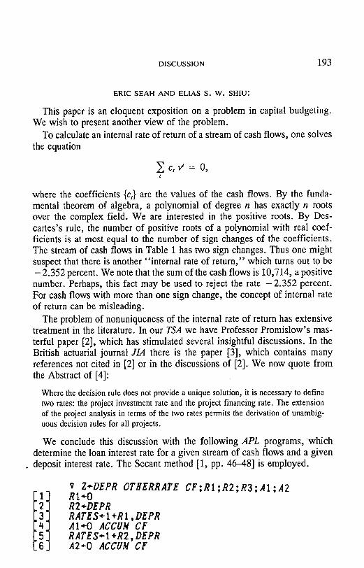
where the coefficients {ct} are the values of the cash flows. By the funda- mental theorem of algebra, a polynomial of degree n has exactly n roots over the complex field. We are interested in the positive roots. By Des- cartes's rule, the number of positive roots of a polynomial with real coefficients is at most equal to the number of sign changes of the coefficients. The stream of cash flows in Table 1 has two sign changes. Thus one might suspect that there is another "internal rate of return," which turns out to be - 2.352 percent. We note that the sum of the cash flows is 10,714, a positive number. Perhaps, this fact may be used to reject the rate - 2 . 3 5 2 percent. For cash flows with more than one sign change, the concept of internal rate of return can be misleading.

The problem of nonuniqueness of the internal rate of return has extensive treatment in the literature. In our TSA we have Professor Promislow's mas- terful paper [2], which has stimulated several insightful discussions. In the British actuarial journal J/A there is the paper [3], which contains many references not cited in [2] or in the discussions of [2]. We now quote from the Abstract of [4]:

Where the decision rule does not provide a unique solution, it is necessary to define two rates: the project investment rate and the project financing rate. The extension of the project analysis in terms of the two rates permits the derivation of unambig- uous decision rules for all projects.

We conclude this discussion with the following APL programs, which determine the loan interest rate for a given stream of cash flows and a given

• deposit interest rate. The Secant method [1, pp. 46-48] is employed•

v Z÷DEPR OTHERRATE R2",-DEPR

! t RAT'S÷I+R1, D'PR 4 A 1 ÷0 ACCIIM CF 5 RATES" I +R2, DEPR

[6-] A2÷O ACCUH CF

CF;R1;R2;R3;A1;A2


l i ! CHECK:÷((1E-6>IA1-A2)^IE-6>IA2)/END R3÷R1-Alx(R2-R1)÷A2-A1 RI÷R2

] AI÷A2 [ 1 1 ] R2÷R3

A2÷O ACCUM CF L14/ ÷CH~CK [15] END:Z+R2

v Z+C ACCUM CF

Z-((CxRATES[I+C>O3)+CF[1])

END:Z+C V

ACCU~ I+CF

For the example in the paper, one would enter 0.07 OTHERRATE -125138 59135 46986 36013 ...

into the computer, which then returns the value 0.1372929808 as the loan interest rate.

REFERENCES

1. BURDEN, R.L. AND FAIRES, J.D. Numerical Analysis. Third Edition. Boston: Prin- die, Weber and Schmidt, 1985.

2. PROMISLOW, S.D. "A New Approach to the Theory of Interest," TSA, XXXII (1980): 53-92; Discussion 93-117.

3. RUSSELL, A.M. AND RICKARD, J.A. "Uniqueness of Non-Negative Internal Rate of Return," Journal of the Institute of Actuaries, CIX (1982): 435--445.

4. TEICHROEW, D., ROBICHEK, A.A., AND MONTALBANO, M. "An Analysis of Cri- teria for Investment and Financing Decisions Under Certainty," Management Science, XII (1965): 151-179.

ROGER E. JOHNSON:

I would like to thank Mr. Paquin for his article; it stimulated my thinking and, I am sure, that of many others.

Mr. Paquin's most important contribution is the concept that a particular cash flow stream can have "depositor status" and "borrower status" at different times and that these statuses do not coincide with cash flows for a given year being positive or negative. His Table 2 illustrates this very ef- fectively.

DISCUSSION 195

Exactly how to use this insight is the problem, however. Some anomalies in Mr. Paquin's approach are discussed below.

There are multiple pairs of lending/borrowing rates. Just as a company would earn 13.73 percent, if it credited 7.00 percent (in Mr. Paquin's example), it also would earn 12.98 percent if it credited 6.00 percent; or it would earn 14.38 percent if it created 8.00 percent. Table A lists several potential pairs of values; Table B (similar to Mr. Paquin's Table 2) demonstrates the accuracy of one of the pairs.

TABLE A

APPROPRIATE PAIRS OF CREDITED/EARNED RATES FOR MR. PAQUIN'S CASH FLOW STREAM

Credited Rate Earned Rate

5.00% 6.00 7.00 8.00 9.00

10.00 11.00 12.00 13.00 14.00 15.00 16.00 17.00 17.78 18.00 19.00 20.00

12.12% 12.98 13.73 14.38 14.94 15.42 15.84 16.22 16.56 16.87 17.14 17.39 17.62 17.78 17.82 18.01 18.17

Note that an IRR of 17.78 percent is equivalent to earning 17.78 percent while crediting 17.78 percent.

When the same cash flow stream repeats itself year after year, the earned/ credited pair changes. Consider the cash flow stream in Mr. Paquin's example. If this stream recurs for five consecutive years (as if an equal amount of the product were sold for the next five years), then the combined cash flow stream is given in Table C. This cash flow stream will earn 14.09 percent when crediting 7.00 percent; this is a different pair than results from the original (nonrecurring) stream. This is demonstrated in Table D.

As the cash flow stream is replicated more and more times, the earned rate approaches 17.78 percent (the IRR) while the credited rate is fixed at 7.00 percent. (For example, with 10 years of replication the earned rate is 15.11 percent; with 20 years it is 17.11 percent).

Note that the IRR is always 17.78 percent, whether or not the cash flow stream is replicated.


TABLE B

CASH FLOW wrrH 14.38% CrL~R6E ON LOANS AND 8.00% CREDIT ON DEPOSITS


(1) ! (2) (3) (4) (5) (6) Calendar Previous Current Interest Interest Balance

Year Balance Receipt or Balance Charged Paid (3)- (4) or t (6)t- 1 Disbursement (1) + (2) (3) x.1438 (3) x .08 (3) + (5)

1986 1987 1988 1989 1990 1991 1992 1993 1994 1995 1996 1997 1998 1999 2000 2001

0 (143,135) (96,080) (56,155) (23,038)

1,246 19,796 33,862 43,865 49,921 52,740 52,942 49,269 42,268 31,895 18,020

(125,138) 59,135 46,986 36,013 24,192 17,084 11,557 6,754 2,358 1,087) 3,720) 7,323)

10,132) '12,735) '15,210) 118,020)

(125,138) (84,000) 49,094) 20,142)

1,154 18,330 31,353 40,616 46,223 48,834 49,020 45,619 39,137 29,533 16,685

0

17,997 12,080 7,060 2,897

0 0 0 0 0 0 0 0 0 0 0 0

0 0 0 0

92 1,466 2,508 3,249 3,698 3,907 3,922 3,650 3,131 2,363 1,335

0

(143,135) (96,080) (56,155) (23,038)

1,246 19,796 33,862 43,865 49,921 52,740 52,942 49,269 42,268 31,895 18,020

0

TABLE C

COMBINED CASH FLOW STREAM

Year Amount

1986 (125,138) 1987 (66,003) 1988 (19,017) 1989 16,996 1990 41,188

Year Amount Year Amount Year Amount

1991 183,410 1996 15,862 2001 (63,420) 1992 135,832 1997 (3,018 2002 (56,097) 1993 95,600 1998 (19,904 2003 (45,965) 1994 61,945 1999 (34,997 2004 (33,230) 1995 36,666 2000 (49,120 2005 (18,020)

The prudent banker's method is not well suited for decision making. Consider two cash flow streams (products or "blocks of business"), one of which earns 13 percent when it credits 7 percent and the other which earns 14 percent when it credits 8 percent. It is not clear which is to be preferred by the company.

Even if the second stream was to earn 13.25 percent when it credits 7 percent, it would not be clear which stream was better. The reason for this is that what matters is not only the rate earned on money invested given a certain credited rate, but also how much is earned and credited. For example, consider the cash flow streams in Table E. Cash flow stream S earns 13.25 percent when it credits 7.00 percent, while T earns 13.00 percent when it credits 7.00 percent. However, S earns 13.33 percent when it credits 8.00 percent, while T earns 13.46 percent when it credits 8.00 percent. Thus, the prudent banker's method will be unable to tell which stream is preferred.

DISCUSSION 197

TABLE D

CASH FLOW WXTH 14.09% CHARGE ON LOANS AND 7.00% CREDIT ON DEPOSITS



Year Balance Disbursement Balance Charged Paid (3) - (4) or t (6)t- 1 (1) + (2) (3) x .1409 (3) x .07 (3) + (5)

1986 1987 1988 1989 1990 1991 1992 1993 1994 1995 1996 1997 1998 1999 2000 2001 2002 2003 2004 2005

0 142,768 238,183 293,436 315,386 312,828 147,651 (13,484 87,864

160,295 210,749 242,474 256,217 252,855 233,108 196,868 142,789 92,760 50,071 18,020

(125,138) (66,003) (19,017) 16,996 41,188

183,410 135,832 95,600 61,945 36,666 15,862 (3,018

(19,904 q34,997 q49,12C 163,42C 56,097 45,965 33,23C 18,02C

,125,138 ,208,771 257,200 276,440 274,198 129,418 (11,819 82,116

149,809 196,961 226,611 239,456 236,313 217,858 183,988 133,448 86,692 46,795 16,841

0

17,630 29,413 36,235 38,946 38,630 18,233 1,665

0 0 0 0 0 0 0 0 0 0 0 0 0

0 0 0 0 0 0 0

5,748 10,487 13,787 15,863 16,762 16,542 15,250 12,879 9,341 6,068 3,276 1,179

0

142,768) ,238,183) 293,4361 315,3861 312,8281 147,651t

13,484 87,864

160,295 210,749 242,474 256,217 252,855 233,108 196,868 142,789 92,760 50,071 18,020

0

TABLE E

PROJECTED CASH FLOWS

Cash Flow Cash Flow Year Stream S Stream T

1986 1987 1988 1989 1990

(1,000) 482 500 469

(215)

(1,000) 776 551 473

(679)

The IRR for stream S is 13.78 percent and stream T is 16.84 percent. It would seem that T is better.

Another way to verify that T is better is to notice that subtracting T from S gives a cash flow stream where there is only earning going on (from the point of view of the company). The S-T stream has an IRR of 10.55 percent. Thus, S is equivalent to T plus some additional investment earning 10.55 percent.

It seems (though I cannot prove it) that a higher IRR implies a better cash flow stream.

In summary, though there are some anomalies in the Prudent Banker's Method, it does get us thinking in terms of depositor and borrower status


within a cash flow stream. Also, it reminds us that IRR means not only the rate earned on investments but also the rate paid on deposits. I hope these insights can be further developed.

S. DAVID PROMISLOW:

Mr. Paquin's example is of interest since it shows that certain types of transactions, discussed in [1] and [2] with somewhat artificial examples, really do occur in practice. These transactions typically show multiple yield rates and Mr. Paquin's example is no exception. In addition to the 17.78 percent yield which Mr. Paquin calculates, there is another yield rate of -2 .35 percent. Yield rates in the interval ( -1 ,0 ) are just as valid as those which are nonnegative. It should be clear that the 17.78 percent yield is not indicative of the worth of the undertaking any more than the - 2.35 percent yield would be.

The calculation of the 13.73 percent rate of return gives a particular value of the function r(i) defined by Teichrow, Robichek, and Montalbano in [2]. Mr. Paquin shows that for the case at hand, r(0.07) = 0.1373. In the terminology of [2], r(i) represents the project investment rate given a project financing rate of i. (In this work the word "project" is used in place of the word "transaction" as used in [1]). For an excellent summary of the material in [2], see the discussion of [1] by Professor James Hickman.

The function r(i) was introduced by the authors of [2] to provide a decision making tool for accepting or rejecting projects. They assume unlimited ac- cess to capital at some fixed rate and stress that they consider each project on its own right and are not attempting to compare one to the other. As an example, if one postulates that this fixed rate is 0.07, then the decision rules of [2] would tell one to undertake the project represented by Mr. Paquin's example since the return of 13.73 percent is more than the 7 percent cost of financing. The same conclusion can be obtained using the methods of [1], without the calculation of r(i), simply by noting that the present value of the transaction is positive when calculated at a rate of 7 percent.

The use of r(i) seems reasonable for the indicated purpose, but I have reservations about interpreting it absolutely as some type of yield rate, or particularly about using it for comparing one transaction with another.

To illustrate, we will facilitate computation by analyzing an easier example, namely that of [1], Example 13. Using the notation of Section III of [1] we consider the transaction

T = ( - 1 , 7 , -6 ) .

This is really just a simpler version of Mr. Paquin's example and it has similar properties. It begins with negative payment(s), followed by positive

DISCUSSION 199

one(s), and then concludes with negative payment(s). It also has two yield rates, namely 0 and 500 percent. Using the formulas given by Professor Hickman in the above reference we can easily calculate that for the transaction T,

6i r(i) = i + i"

The decompositions discussed in [1, Section VIII], and shown in Example 13 of that paper can be used to illustrate the interpretation of r(i). Note that

6 1 + r(i) + 1 + i = 7.

Then for any rate i (the "deposit" rate in Mr. Paquin's terminology, the "financing" rate in the terminology of [2], and the "borrowing" rate in the terminology of [1]), we can write

T = R + S

where

6 S = (0, 1 + i ' - 6) consists of borrowing funds at rate i

and

R = ( - 1, 1 + r(i)) consists of investing funds at rate r(i).

This is fine, but before one uses this to attribute some special significance to r(i), it should be noted that the rates in such decompositions are far from unique and that there are many other possible investments returns which can be shown for the same deposit rate. For example, if i = 100 percent, then r(i) = 300 percent. However, we can also write

T = ( - 1 , 3 , 2 ) + (0 ,4 , - 8 ) ,

which again consists of borrowing at 100 percent, but in this case investing it at 256.15 percent, the yield of the first summand. I think it is a reasonable conjecture that r(i) is the highest rate of return possible in such a decom- position with deposit rate i, but I have not verified this in all cases.

Difficulties can arise if one tries to use r(i) to compare two different transactions. Suppose we postulate i -- 100 percent and accordingly consider the yield on T to he r(1) = 3. Now consider the transaction


V = ( - 1 , 0, 15),

which had a unique yield of something less than 300 percent (it would be exactly 300 percent if the payment of 15 were 16), independent of any deposit rate i. Does this mean that one would always choose T, if required to pick one of the transactions T or V? Clearly this cannot be the case. Since T - V = (0, 7, - 2 1 ) , an individual would choose T only if he/she were willing to accept a unit in exchange for a repayment of 3 units one period later.

The message here is that, as emphasized in [1], one should not really be talking about yield rates at all when analyzing a mixed transaction compris- ing elements of both borrowing and lending, or both financing and investment.

REFERENCES

1. PROMISLOW, S.D. "A New Approach to the Theory of Interest," TSA, XXXII(1980): 53-92; Discussion 93-117.

2. TEICHROW, D., ROBICHEK, A.A., AND MOWrALBANO, M. "An Analysis of Criteria for Investment and Financing Decisions Under Certainty," Management Science, XII (1965): 151-179.

BRADLEY E. BARKS"

Mr. Anderson's concept [1] of rate of return on investment (ROI) has been a preferred measure of profitability for many years because of its sim- plicity and comparative value. It attempts to summarize the entire profit stream of a product into a single number independent of product type. Mr. Paquin deserves thanks for his valuable insight into some of the flaws that exist in this profit measure as it is currently used and for his extension of the original methodology to provide consistency with Mr. Anderson's original criteria in certain problem situations. This discussion will comment on the following:

1. similarities and differences between Mr. Paquin's and Mr. Anderson's methodol- ogies,

2. the determination of the "savers" rate, and 3. the concepts of "equity at risk" and "equity at work," including an example.

In his 1959 paper, Mr. Anderson presents (on page 365) the criteria that his ROI profit measure is based on:

1. that the amount of profit be related to the amount of surplus which must be invested to acquire that profit and expressed as a yield rate on the investment; and

2. that the yield rate be associated with the degree of risk incurred on the type of investment made.

DISCUSSION 201

It is important to note that many problems that actuaries have been con- fronted with over the years have been caused by blind application of the method and not by ambiguity of the criteria.

Similarities

In order to more easily see the similarities between the Anderson ROI and the Prudent Banker's Rate of Return on Investment (PBROI), I would propose an alternative method as defined in Table 2': Column 2: Discount cash flows (CF) using the savers interest rate (7 per-

cent) to the greatest duration t where the fund balance is non- positive using the following formula (equivalent to that used in Mr. Paquin's paper).

Fund, = Fundt + l/(1.07) - CF,

Column 3: Calculate the Anderson ROI from issue to the year determined in Column 2 using negative Fund, as the CF in the last year.

TABLE 2'

(1) (2) (3) (4) (s) Cash Flow Cash Flow Cash Flow Cash Flow

Calendar Discounted Used in Discounted Used in Year Cash at 7% to Anderson at 9% to Anderson

t Flows Year t ROI Year t ROI

1986 1987 1988 1989 1990 1991 1992 1993 1994 1995 1996 1997 1998 1999 2000 2001

Anderson ROI

- 125,138 59,135 46,986 36,013 24,192 17,084 11,557 6,754 2,358

- 1,087 -3,720 -7,323

-10,132 -12,735 -15,210 -18,020

-16,306 - 151,345

-98,665 -55,297 -20,634

3,808 22,354 36,285 46,051 51,798 54,261 54,079 50,029 42,689 32,051 18,020

- 125,138 59,135 46,986 36,013 20,634

13.73%

- 14,316 - 152,005 - 101,228

-59,124 -25,191

- 1,089 17,434 31,601 41,806 48,139 51,287 51,848 48,532 41,856 31,742 18,020

-125,138 59,135 46,986 36,013 24,192

1,089

14.94%

The result shown in Table 2', 13.73%, is identical to the result in Table 2 of Mr. Paquin's paper. I am not proposing this method, called PBROI', as a replacement for PBROI because this method will work only when the fund balance changes from negative to positive no more than once. However, PBROI' does illustrate that the PBROI method can be viewed as the traditional Anderson ROI limited to the period of time over which the company


can recover its investment. The receipts from 1991 through 1994 are not included in the PBROI' calculation because they are required to fund the disbursements from 1995 through 2001 and, therefore, are not a return on the original investment of CF. In other words, before 1991 the company invests its CF in the line of business and should earn a risk rate of return on the CF. However, after 1990 the company acts merely as a custodian of funds needed to pay future disbursements and should credit substantially less than the risk rate of return on these funds. Thus, PBROI is consistent with Mr. Anderson's second criterion requiring the yield rate to reflect the degree of risk imposed on the insurer.

I emphasize that the Anderson ROI need not be "turned on its head," but simply modified to reflect the actual risk the company is subjected to. In fact, identical results are obtained by discounting as are obtained by accumulating. The following describes a discounting methodology that is identical in result to Mr. Paquin's.

Fundt = Fund~+l / (1+i) - CF,

where

.the savers rate when Fund,+~ > 0 [ i

~the risk rate of return when Fund,+~ < 0

and Fund , + 1 = 0 = Fund at end of year last CF occurs (solved by interval bisection for the risk rate of return such that Fund1 = 0).

In spite of the above demonstration I prefer Mr. Paquin's accumulation methodology because it is intuitively simpler.

Differences

Mr. Paquin makes two significant departures from Mr. Anderson's methodology. First, PBROI is based on the cash flows on a block of business while the Anderson ROI is based on book profit as defended by Mr. An- derson [1]. I am not sure of the reason for this departure but I believe that PBROI will work equally well if book profits are used. Second, as Mr. Paquin points out, the insurer will most likely be able to invest its assets at a rate in excess of the savers rate of 7 percent. Clearly, a banker makes a profit on its savings accounts as well as its loans, but PBROI is insensitive to the profits when the fund is positive (savings). The Anderson ROI, however, would be sensitive to all sources of profit.

DISCUSSION 203

The Savers Rate

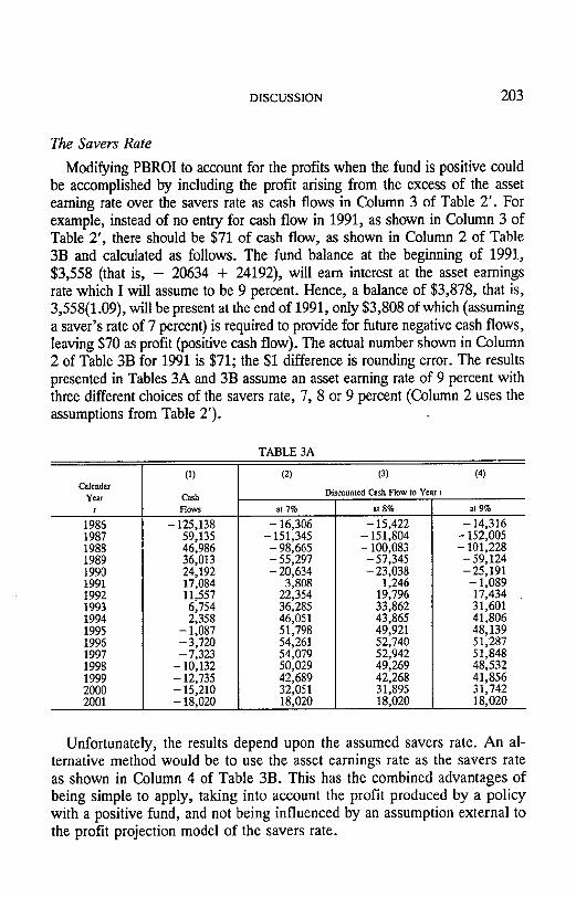
Modifying PBROI to account for the profits when the fund is positive could be accomplished by including the profit arising from the excess of the asset earning rate over the savers rate as cash flows in Column 3 of Table 2'. For example, instead of no entry for cash flow in 1991, as shown in Column 3 of Table 2', there should be $71 of cash flow, as shown in Column 2 of Table 3B and calculated as follows. The fund balance at the beginning of 1991, $3,558 (that is, - 20634 + 24192), will earn interest at the asset earnings rate which I will assume to be 9 percent. Hence, a balance of $3,878, that is, 3,558(1.09), will be present at the end of 1991, only $3,808 of which (assuming a saver's rate of 7 percent) is required to provide for future negative cash flows, leaving $70 as profit (positive cash flow). The actual number shown in Column 2 of Table 3B for 1991 is $71; the $1 difference is rounding error. The results presented in Tables 3A and 3B assume an asset earning rate of 9 percent with three different choices of the savers rate, 7, 8 or 9 percent (Column 2 uses the assumptions from Table 2').

TABLE 3A

Calendar Year

1

1986 1987 1988 1989 1990 1991 1992 1993 1994 1995 1996 1997 1998 1999 2000 2001

(1)

Cash Flows

- 125,138 59,135 46,986 36,013 24,192 17,084 11,557 6,754 2,358

-1,087 -3,720 -7,323

-10,132 -12,735 - 15,210 - 18,020

( 2 ) ( 3 ) ( 4 )

Discounted Cash Flow to Year t

at 7 % at 8 %

-15,422 - 151,804 - 100,083 -57,345 -23,038

1,246 19,796 33,862 43,865 49,921 52,740 52,942 49,269 42,268 31,895 18,020

- 16,306 - 151,345 -98,665 -55,297 -20,634

3,808 22,354 36,285 46,051 51,798 54,261 54,079 50,029 42,689 32,051 18,020

at 9%

-14,316 - 152,005 - 101,228 -59,124 -25,191

- 1,089 17,434 31,601 41,806 48,139 51,287 51,848 48,532 41,856 31,742 18,020

Unfortunately, the results depend upon the assumed savers rate. An alternative method would be to use the asset earnings rate as the savers rate as shown in Column 4 of Table 3B. This has the combined advantages of being simple to apply, taking into account the profit produced by a policy with a positive fund, and not being influenced by an assumption external to the profit projection model of the savers rate.


TABLE 3B

Calendar Year

t

1986 1987 1988 1989 1990 1991 1992 1993 1994 1995 1996 1997 1998 1999 2000 2001

Anderson ROI

(1)

Cash Flows

- 125,138 59,135 46,986 36,013 24,192 17,084 11,557 6,754 2,358

-1,087 -3,720 -7,323

- 10,132 - 12,735 - 15,210 - 18,020

(2)

at 7%

- 125,138 59,135 46,986 36,013 20,634

71 418 678 861 968

1,014 1,011

935 798 599 337

14.65%

(3)

Cash Flow Used in Anderson ROI

at 8%

- 125,138 59,135 46,986 36,013 23,038

12 183 314 406 462 488 490 456 391 295 167

14.81%

(4)

at 9%

- 125,138 59,135 46,986 36,013 24,192

1,089 0 0 0 0 0 0 0 0 0 0

14.94%

At Work vs. At Risk

Finally, Mr. Paquin suggests a distinction between the terms "equity at work" and "equity at risk." I am intrigued by this concept and would like to try to clarify some of the issues he has raised through an example as follows:

Monthly Premium Annual Renewable Term Product • Cash Value = 0 • Reserves = 0 • Gross Premium = $0.50 per $1,000 of face amount per month • Expected Deaths = 0.4 per 1,000 per month • Commission = 40% of premiums in 1st year (paid monthly).

What is "at work" and "at risk" on a policy with a death benefit of $100,000 and a gross premium of $50 per month? The balance sheet for 1,000 such policies just before the seventh monthly premium is collected is shown below, assuming the following: no lapses; actual deaths equal expected deaths (occurring at the end of the month); an asset earning rate of 9 percent; and initial assets of $200,000.

Invested Assets

Total

149,029"

149,029

Liabilities I 0 Surplus 149,029

149,029

*Initial Capital + Premium - Commission - Deaths (with interest)

200,000 (1.0440) + [50,000(1 - 0.4)(1.0072) - 40,000] S,~

DISCUSSION 2 0 5

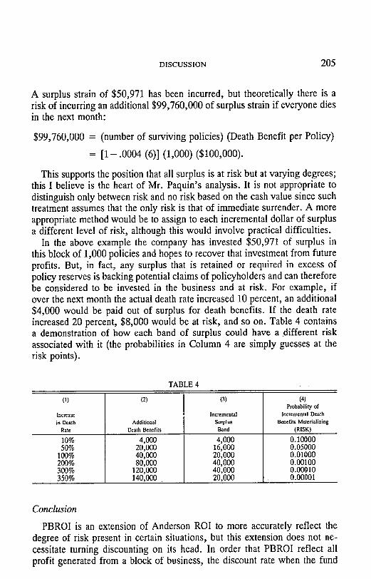
A surplus strain of $50,971 has been incurred, but theoretically there is a risk of incurring an additional $99,760,000 of surplus strain if everyone dies in the next month:

$99,760,000 = (number of surviving policies) (Death Benefit per Policy)

= [1- .0004 (6)] (1,000) ($100,000).

This supports the position that all surplus is at risk but at varying degrees; this I believe is the heart of Mr. Paquin's analysis. It is not appropriate to distinguish only between risk and no risk based on the cash value since such treatment assumes that the only risk is that of immediate surrender. A more appropriate method would be to assign to each incremental dollar of surplus a different level of risk, although this would involve practical difficulties.

In the above example the company has invested $50,971 of surplus in this block of 1,000 policies and hopes to recover that investment from future profits. But, in fact, any surplus that is retained or required in excess of policy reserves is backing potential claims of policyholders and can therefore be considered to be invested in the business and at risk. For example, if over the next month the actual death rate increased 10 percent, an additional $4,000 would be paid out of surplus for death benefits. If the death rate increased 20 percent, $8,000 would be at risk, and so on. Table 4 contains a demonstration of how each band of surplus could have a different risk associated with it (the probabilities in Column 4 are simply guesses at the risk points).

TABLE 4

(1)

Increase in Death

Rate

10% 50%

100% 200% 300% 350%

(z)

Additional Death Benefits

4,000 20,000 40,000 80,000

120,000 140,000

(3)

Incremental Suq~lus Band

4,000 16,000 20,000 40,000 40,000 20,000

(4) Probability of

Incremental Death Benefits Materializing

(RISK)

0.10000 0.05000 0.01000 0.00100 0.00010 0.00001

Conclusion

PBROI is an extension of Anderson ROI to more accurately reflect the degree of risk present in certain situations, but this extension does not ne- cessitate turning discounting on its head. In order that PBROI reflect all profit generated from a block of business, the discount rate when the fund


balance is positive must be the asset earnings rate. Finally, in order for ROI to have real meaning, management must know what risks are associated with the activities in question. Unfortunately, surplus cannot be partitioned into that which is at risk and that which is not unless some future events are not probabilistic. Instead, every layer of surplus is subject to a chance (no matter how slim) that it may be dissolved through contractual claims within a given period of time. The " top" layers of surplus (those which are liquidated first) are at much higher risk than are the "bottom" layers, which would only be at risk in an extreme catastrophe. This leaves us with the tools of utility theory to try to equate a broad continuum of risk to dollars of invested surplus. Given the recent volatility of the financial markets and the potential of the AIDS epidemic, it is clear that the insurance environment is becoming more risky. I would expect that in the not-too-distant future, all pricing will be adjusted for the risk profile of the insurer and that the technique for adjusting profit measures for risk will have to be more fully developed.

REFERENCE

1. ANDERSON, J.C.H. "Gross Premium Calculations and Profit Measurement for Non- participating Insurance," TSA, XI (1959): 357-394; Discussion 395-420.

COURTLAND C. SMITH:

Mr. Paquin questions the decision-making value of conventional return- on-investment (ROI) analysis in situations where cash flows are mixed, that is, sometimes negative and sometimes positive as in his Table 1. I have related questions. Ever since my days of preparing coinsurance quotations for a reinsurer, I have wondered at the low ROI's which some of my com- petitors (and sometimes we ourselves) were willing to accept in the heat of competitive battle. At the time, we usually managed to avoid troublesome situations by insisting on a mortality risk charge, a discounting rate higher than most of the market, and a positive spread between the discounting rate and the earnings rate. Generally, we also tried to achieve a positive net balance by that duration in which recapture was first permitted.

Mr. Paquin proposes that in evaluating mixed cash flows we use one rate for positive credit balances, and another, much higher, rate for negative balances, just as a prudent banker charges more on loans than he credits on deposits. To be sure, Mr. Paquin's illustrative set of cash flows includes net credit balances, whereas many bankers would gladly offer to lend $1,000 at 7 percent on the security of a $2,000 balance in a 5 percent savings account if the depositor were unwilling to withdraw any funds.

The message may be that we should base our investment decisions on securing two preconditions:

DISCUSSION 207

1. a sufficiently high return on loans or positive balances (say, over 15 percent) and 2. a threshold spread (say, over 2 percent) between this return and the rate credited

on net deposits or positive balances.

If SO, we have a problem: There is no unique solution that satisfies these conditions. We can produce an indefinitely large number of pairs of charge and crediting rates, of which some would give a "Yes, Invest" decision and others a " N o . "

Column 2 of Table 1 of this discussion contains the projected mixed cash flow in Mr. Paquin's illustration and the conventional ROI of 17.778 percent that yields a zero final balance. Two illustrative loan rates that exceed 15 percent with spread greater than 2 percent are displayed in Tables 2 and 3. Surprisingly, the higher loan return rate is associated with an increased deposit crediting rate. In Tables 1-3 the cash flow balance becomes positive in the sixth year.

The developments in Tables 4 and 5 show inadequate loan return rates (under 15 percent). Interestingly, the balance becomes positive earlier -- in the fifth year. The illustration in Table 6 shows a 4.752 percent loan return rate with a zero deposit crediting rate, and a positive balance still earlier - - in the fourth year.

T h e example of Table 7 shows that a 20 percent crediting rate on net deposits is associated with a return on loans of 18.174 percent, a return even greater than the conventional 17.778 percent ROI. Also, the ROI for this set of mixed cash flows at simple interest is only 0.57 percent a year. This ROI suggests that these cash flows represent a poor investment.

The results of this analysis are summarized in Table 8. Admittedly, if the rate to be credited on net positive balances is dictated by the market, then the return on negative balances is uniquely determined. However, if we decide to make the crediting rate more attractive, it would take longer to recover our initial investment or loan, but our calculated return on that investment would increase. Is this reasonable?

More generally, can any single figure measure prospective return on investment in a way that it can be used in sole support of investment and other risk-taking decisions?

TABLE 1

CASH FLOW WITH j = 17.778137% CHARGE ON LOANS AND

i = 17.778137% CREDrr ON DEPOSITS FINAL BAL. = -- 0.015920

Start of Year End of Year


Year Balance Disbursement Balance Charged Paid (3)- (4) t (6)t- 1 (1)+(2) -(3)*j,> =0 (3)*i,> =0 +(5)

1986 1987 1988 1989 1990 1991 1992 1993 1994 1995 1996 1997 1998 1999 2000 2001

Net PV@

0 147,385) 103,939) (67,079) (36,589) (14,601)

2,925 17,057 28,044 35,807 40,892 43,781 42,939 38,640 30,510 18,020

17.778%

(125,138) 59,135 46,986 36,013 24,192 17,084 11,557 6,754 2,358 1,087) 3,720 7,323'

110,132 ' 112,735' q15,210) t18,020)

0

(125,138t 88,250p 56,953 t 31,066t 12,397p 2,483

14,482 23,811 30,402 34,720 37,172 36,458 32,807 25,905 15,300

(o)

22,247 15,689 10,125 5,523 2,204

0 0 0 0 0 0 0 0 0 0 0

0 0 0 0 0

442 2,575 4,233 5,405 6,172 6,609 6,481 5,832 4,605 2,720

0

147,385, 103,939, (67,079, (36,589, (14,601,

2,925 17,057 28,044 35,807 40,892 43,781 42,939 38,640 30,510 18,020

(o)

TABLE 2


i = 15.000000% CREDIT ON DEPOSITS FINAL BAL. = -- 0.002339

Start of Year End of Year (I) (2) (3) (4) (5) (6)

Calendar Previous Receipt or Current Interest Interest Balance Year Balance Disbursement Balance Charged Paid (3) - (4)

t (6)t- 1 (1)+(2) -(3)*j,> =0 (3)*i,> =0 +(5) 1986 1987 1988 1989 1990 1991 1992 1993 1994 1995 1996 1997 1998 1999 2000 2001

Net PV@

0 146,592) 102,451) (64,975) (33,927) (11,404)

6,532 20,802 31,690 39,155 43,778 46,067 44,555 39,587 30,880 18,020

17.778%

(125,138) 59,135 46,986 36,013 24,192 17,084 11,557 6,754 2,358

I 1,087 3,720' 7,323'

q 10,132' q 12,735) q 15,210) q 18,020)

0

(125,138) (87,457) (55,465) (28,962)

(9,735) 5,680

18,089 27,556 34,048 38,068 40,058 38,744 34,423 26,852 15,670

(o)

21,454 14,994 9,509 4,965 1,669

0 0 0 0 0 0 0 0 0 0 0

0 0 0 0 0

852 2,713 4,133 5,107 5,710 6,009 5,812 5,163 4,028 2,350

0

146,592) 102,451) (64,975) (33,927) (11,404)

6,532 20,802 31,690 39,155 43,778 46,067 44,555 39,587 30,880 18,020

(o)

208

TABLE 3

CASH FLOW wrrH j = 15.416222% CHARGE ON LOANS AND

i = 10.000000% CREOrr ON DEPOSITS FinAL BAL. = 0.0010937



Year Balance Disbursement Balance Charged Paid (3 ) - (4 ) t ( 6 ) ' - 1 (1)+(2) -(3)*/ ' ,> = 0 (3)*i,> = 0 +(5)

1986 1987 1988 1989 1990 1991 1992 1993 1994 1995 1996 1997 1998 1999 2000 2001

0 (144,430) (98,444) (59,391) (26,982) (3,220) 15,251 29,489 39,867 46,447 49,896 50,794 47,818 41,455 31,592 18,020

(125,138) 59,135 46,986 36,013 24,192 17,084 11,557 6,754 2,358 1,087 3,720 7,323'

,10,132 ,12,735 15,210 18,020

(125,138p (85,295~ (51,4581 (23,3781 (2,7901 13,864 26,808 36,243 42,225 45,360 46,176 43,471 37,686 28,720 16,382

0

19,292 13,149 7,933 3,604

430 0 0 0 0 0 0 0 0 0 0 0

0 0 0 0 0

1,386 2,681 3,624 4,222 4,536 4,618 4,347 3,769 2,872 1,638

0

(144,4301 98,4441 59,3911 26,9821 (3,220) 15,251 29,489 36,867 46,447 49,896 50,794 47,818 41,455 31,592 18,020

0

TABLE 4

CASH FLOW WITH j = 13.729298% CHARGt= ON LOANS AnD

i = 7.000000% CREDIT ON DEPOSITS FINAL BAL. = 0.0006697


(1) (2) (3) (4) (5) (6) Calendar Previous Receipt or Current Interest Interest Balance -

Year Balance Disbursement Balance Charged Paid (3) - (4) t ( 6 ) ' - 1 (1)+(2) - (3 )* j ,> = 0 (3) ' i ,> •O +(5)

1986 1987 1988 1989 1990 1991 1992 1993 1994 1995 1996 1997 1998 1999 2000 2001

0 (142,319) (94,604) (54,156) (20,634)

3,808 22,354 36,285 46,051 51,798 54,261 54,079 50,029 42,689 32,051 18,020

(125,138) 59,135 46,986 36,013 24,192 17,084 11,557 6,754 2,358 I,087) 3,720) 7,323)

,10,132 ,12,735 ,15,210 ,18,020

(125,138) (83,184) (47,618) (18,143) (3,558) 20,892 33,911 43,039 48,409 50,711 50,541 46,756 39,897 29,954 16,841

0

17,181 11,421 6,538 2,491

0 0 0 0 0 0 0 0 0 0 0 0

0 0 0 0

249 1,462 2,374 3,013 3,389 3,550 3,538 3,273 2,793 2,097 1,179

0

(142,319) (94,604) (54,156) (20,634)

3,808 22,354 36,285 46,051 51,798 54,261 54,079 50,029 42,689 32,051 18,020

0

209

TABLE 5


i = 3.000000% CREDIT ON DEPOSITS FINAL BAL. = 0.001458

Calendar Year

t

1986 1987 1988 1989 1990 1991 1992 1993 1994 1995 1996 1997 1998 1999 2000 2001

(1) Previous Balance (6)t- 1

Start of Year

(2) Receipt or

Disbursement

(3) Current Balance (1)+(2)

0 (125,138) (125,138) (137,575) 59,135 (78,440) (86,235) 46,986 (39,249) (43,150) 36,013 (7,137) (7,846) 24,192 16,346 16,836 17,084 33,920 34,938 11,557 46,495 47,890 6,754 54,644 56,283 2,358 58,641 60,400 (1,087 59,313 61,093 (3,720 57,373 59,094 (7,323 51,771 53,324 10,132 43,192 44,488 ~12,735 31,753 32,705 '15,210 17,495 18,020 118,020 (0)

(4) Interest

Charged -(3)'j,> =0

12,437 7,796 3,901

709 0 0 0 0 0 0 0 0 0 0 0 0

End of Year

(5) Interest

Paid (3)*i, > = 0

0 0 0 0

490 1,018 1,395 1,639 1,759 1,779 1,721 1,553 1,296

953 525

0

(6) Balance (3)- (4)

+(5) (137,575) (86,235) (43,150) (7,846) 16,836 34,938 47,890 56,283 60,400 61,093 59,094 53,324 44,488 32,705 18,020

(o)

TABLE 6

CASH FLOW WITH

j = 4.751858% CHARGE ON LOANS AND i = 0.000000% CREDIT ON DEPOSITS

FINAL BAt.. --.---- 0.0003793



Year Balance Disbursement Balance Charged Paid (3) - (4) t (6), ' -I (1)+ (2) - (3)*j,> =0 (3) ' i ,> =0 +(5)

1986 1987 1988 1989 1990 1991 1992 1993 1994 1995 1996 1997 1998 1999 2000 2001

Net PV@

0 (131,084) (75,368) (29,731)

6,282 30,474 47,558 59,115 65,869 68,227 67,140 63,420 56,097 45,965 33,230 18,020

-2.3517%

(125,138) 59,135 46,986 36,013 24,192 17,084 11,557 6,754 2,358 1,087 3,720 7,323

10,132 12,735 15,210 18,020

0

(125,138) (71,949) (28,382)

6,282 30,474 47,558 59,115 65,869 68,227 67,140 63,420 56,097 45,965 33,230 18,020

0

5,946 3,419 1,349

0 0 0 0 0 0 0 0 0 0 0 0 0

(131,084) (75,368) (29,731)

6,282 30,474 47,558 59,115 65,869 68,227 67,140 63,420 56,097 45,965 33,230 18,020

0

210

TABLE 7


i = 20.000000% CREDIT ON DEPOSITS FINAL BAL. = --0.019020



Year Balance Disbursement Balance Charged Paid (3)- (4) t (6)t- 1 (1)+(2) - (3)*j,> =0 (3)*i,> =0 +(5)

1986 1987 1988 1989 1990 1991 1992 1993 1994 1995 1996 1997 1998 1999 2000 2001

Net PV@

0 147,880) 104,873) (68,408) (38,282) (16,651)

520 14,493 25,496 33,425 38,805 42,102 41,735 37,924 30,227 18,020

17.7780%

(125,138) 59,135 46,986 36,013 24,192 17,084 11,557 6,754 2,358 1,087) 3,720) 7,323)

q10,132) ~12,735) t15,210) t18,020)

0

Net N 10,714 Years Y 15

Principal P 125,138 ROI(simpl) = N/(Y*P) 0.57%

(125,138 88,745 57,887 32,395

(14,090 433

12,077 21,247 27,854 32,338 35,085 34,779 31,603 25,189 15,017

(0)

t 22,742 16,128

I 10,520 P 5,887 P 2,561

0 0 0 0 0 0 0 0 0 0 0

0 0 0 0 0

87 2,415 4,249 5,571 6,468 7,017 6,956 6,321 5,038 3,003

0

147,880 104,873 68,408 38,282 16,651

520 14,493 25,496 33,425 38,805 42,102 41,735 37,924 30,227 18,020

(0)

TABLE 8

ILLUSTRATIVE PAIRS OF CHARGE AND CREDITING RATES WHICH PRODUCE A ZERO FINAL BALANCE

FOR THE PROJECTED CASH FLOWS IN MR. PAQUIN'S TABLE 1

j i Year Investment Charge on Credit on Flow Decision

Source Negative Positive Spread Becomes (Yes iffj> 15% Table Balances Balances j - i Positive a n d j - i > 2%)

17.778137% 17.144511% 15.416222% 13.729298% 9.938332% 4.751858%

18.173640%

17.778137% 15.000000% 10.000000% 7.000000% 3.000000% 0.000000%

20.000000%

0.00% 2.14% 5.42% 6.73% 6.94% 4.75%

- 1 . 8 3 %

No Yes Yes No No No No

Return on Investment (Simple Interest)

0.57% No

211


THOMAS M. MARRA:

The problem of how to handle book profit strcams alternating between positive and negativc amounts is indeed pertincnt to many of the life and annuity products of the 1980s. Mr. Paquin's Prudent Banker's Method offers onc possible responsc to this dilemma, and this method is in fact currcntly in use within our industry.

My intuition, however, tclls me that the Prudent Bankcr's Method may be unduly conservative. The crux of this assertion lies in the fact that when thc current balancc becomcs positive, it is accumulated at thc much lower, borrowcr's rate (7 percent in Mr. Paquin's example). Mr. Paquin statcs that

Nothing prevcnts thc insurer from investing its positive ba lances . . . a t morc than 7 percent annually if it can.

Would it not be more appropriate to assume that the insurer can in fact invest thcse positive balances (if not distributing them as dividends) at a ratc higher than 7 perccnt (perhaps at the insurer's required ROI ratc)? It would seem to me that the insurer's very existence depends on an expectation of ratcs of return above the borrower's rate.

An alternative approach to the Prudent Banker's Method is what I call the Consolidated Transaction Method. The insurer's management faced with the book profit results in Mr. Paquin's Table 1 is most likely also involved in other product lines that produce a more normal book profit pattern, that is, a single negative amount rcpresenting an initial investment followed by strictly positive amounts representing the income from that investment. The Con- solidated Transaction Method simply allows management to consolidate among product lines to assess the results of the abnormal book profit product. In csscncc, it is a model company responsc to this pricing dilemma.

As a very simple example of the application of the Consolidated Trans- action Method, consider a company offering only two products, one producing the results of Mr. Paquin's Table 1, and the second producing the results of Example 2, shown below. The consolidated results are also shown:

DISCUSSION 213

CONSOLIDATED TRANSACTION METHOD PROJECTED BOOK PROFITS

Table I Example 2 Consolidated Transaction Year Book Profits Book Profits Book Profits

1986 1987 1988 1989 1990 1991 1992 1993 1994 1995 1996 1997 1998 1999 2000 2001 ROI

- 125,138 59,135 46,986 36,013 24,192 17,084 11,557 6,754 2,358

- 1,087 -3,720 -7,323

-10,132 -12,735 - 15,210 -18,020

- 102,825 20,000 20,000 20,000 20,000 20,000 20,000 20,000 20,000 20,0O0 20,000 20,000 20,000 20,000 20,000 20,000

17.78%

- 227,962 79,135 66,986 56,013 44,192 37,084 31,557 26,754 22,358 18,913 16,280 12,677 9,868 7,265 4,790 1,980

17.78%

As can be seen, the amounts in the Consolidated Transaction Book Profits column are once again normal, and the consolidated ROI exactly equals that of Example 2, 17.78 percent. As such, if the insurer's required ROI is say 15 percent, the Consolidated Transaction Method would conclude that the book profit results of Table 1 are acceptable. The Prudent Banker 's Method, producing a 13.73 percent return, would deem the Table 1 results unacceptable.

Of course, there are hazards inherent in the Consolidated Transaction Method which must be considered:

1. The relative magnitudes of the two (or more) cash flow streams must be similar to avoid the consolidated results being overly biased toward the stream of larger magnitude. For this reason, it may be preferable to perform the consolidated analysis on a unit amount basis.

2. There is no assurance that the consolidated stream will be normal, or for that matter that the insurer has enough normal product lines to result in a normal consolidated transaction.

3. Obviously management would much prefer each product line to stand on its own, and not have one line be overly dependent on the results of another line.

4. The implications of the abnormal book profit stream on future cash flow and surplus requirements will need to be considered in assessing the desirability of the abnormal product line.

Obviously the Consolidated Transaction Method presents some undesir- able characteristics. However, I believe that use of the Prudent Banker 's Method also presents pitfalls. Perhaps the preferable approach is to consider both methods (and perhaps to also consider other methods such as straight present value [of book profits] analysis) and, recognizing the shortcomings of each, make an overall assessment regarding the acceptability or unac- ceptability of the abnormal book profit product line.


(AUTHOR'S REVIEW OF DISCUSSION) CLAUDE Y. PAQUIN"

While paying this paper the compliment of their attention and their discussions, the ten discussants have brought up matters which are interesting and thought-provoking in their own right. The contribution of bibliographical materials by a few of them will no doubt prove helpful to many readers.

A prudent banker is also practical. Thus the existence of a possible negative yield for the illustrated cash flow is deemed of no moment for the purposes of this paper. By no means is this comment intended to belittle the various learned approaches developed by theoreticians in the fields of finance and economics. The point of the paper is that no one should allow himself to be so overwhelmed by theory as to disregard reality, and reality, when confronting an innocuous cash flow such as the one illustrated in the paper, is that even though the "rate of return" on such a cash flow may be 17.78 percent, it is not always "returned" to the person to whom one might, at first glance, assume it is.

A prudent banker would likely consider a table such as Table 2 in the paper and ask himself, "Can I safely promise to pay 7 percent, starting five years hence and for eleven consecutive years, on the positive balances shown in column (3)?" Before he could answer that, he would of course consider the likelihood of his being able to lend the future positive balances at an effective net annual rate of no less than 7 percent.

The paper clearly establishes that, for the example given, 17.78 percent is not the annual rate of return which the initial investor is getting; it is the rate which both he and the other party (borrower-depositor) are getting, each in his turn. In the face of the conceptual difficulties presented by this relatively simple problem, should one despair and conclude that "one should not really be talking about yield rates at all when analyzing this type of mixed transaction"? In a capitalistic world conditioned to quantifying financial results in terms of yield, that may not yet be practical. The paper's overriding message counseling against self-delusion remains valid.

It can be delusive to combine separate cash flows before analyzing them. Would not a corporation which always combines the accounting losses of one division with the profits of another before looking at the overall figures delude itself about the real profitability of both? (If neither division can function without the other, the combination is proper; otherwise it is delusive.)

An unfortunate feature of the paper is that what it teaches not to do overshadows its positive message. In other words, it raises more questions than it solves. That a paper which is inherently practical should turn out so philosophical is just another irony of life.

cash flow analysis by the prudent banker's of society of actuaries 1987 vol. 39 cash flow...

Documents