case network reports - sustaining low inflation in ukraine
TRANSCRIPT
CASE Reports
Sustaining Low Inflationin Ukraine
Volodymyr HryvnivMalgorzata Jakubiak
Mykyta MykhaylychenkoOksana Novoseletska
Wojciech PaczynskiPrzemyslaw Wozniak
Edited by Malgorzata Jakubiak
Warsaw 2005
No.
63/
2005
Center for Social and Economic Research
CASE Reports No. 63 2
The views and opinions expressed here reflect the authors’ point of view and not necessarily those of the CASE. This publication was made possible through support provided by the Poland-America-Ukraine Cooperation Initiative (PAUCI), financed by the U.S. Agency for International Development (USAID), under the terms of Cooperative Agreement No. 03-0185-150 The opinions expressed herein are those of the authors and do not necessarily reflect the views of USAID, Freedom House or PAUCI. Keywords: Ukraine, transition, monetary policy, inflation, core inflation, financial market, monetary transmission. © CASE – Center for Social and Economic Research, Warsaw 2005 Graphic Design: Agnieszka Natalia Bury ISBN: 83-7178-392-2 Publisher: CASE – Center for Social and Economic Research 12 Sienkiewicza, 00-944 Warsaw, Poland tel.: (48 22) 622 66 27, 828 61 33, fax: (48 22) 828 60 69 e-mail: [email protected] http://www.case.com.pl/
CASE Reports No. 63 3
Contents
Chapter 1: Sustaining Low Inflation in Ukraine. Overview.............................................6 Małgorzata Jakubiak
1. Introduction ........................................................................................................................... 6 2. Background ........................................................................................................................... 6 3. Rationale for changing nominal anchor................................................................................. 7 4. Research in this volume........................................................................................................ 8 References................................................................................................................................ 9
Chapter 2: Evolution of Price Changes in Ukraine in 1992-2005 .................................10 Małgorzata Jakubiak
1. Introduction ......................................................................................................................... 10 2. 1991-1994: first price and trade liberalisation ..................................................................... 10 3. 1995-1998: gradual stabilisation ......................................................................................... 14 4. 1998-2005: macroeconomic stabilisation and post-crisis expansion .................................. 16 5. Structure of consumption .................................................................................................... 19 6. Summary............................................................................................................................. 20 References.............................................................................................................................. 20
Chapter 3: Polish Disinflation Experience: 1990-2004..................................................22 Przemysław Woźniak
1. Introduction ......................................................................................................................... 22 2. The Initial Stabilization 1990-1992 ...................................................................................... 22 3. Eclectic Monetary Policy 1993-1998 ................................................................................... 27 4. Direct Inflation Targeting ..................................................................................................... 31 5. Changes in relative prices and inflation structure ............................................................... 35 References.............................................................................................................................. 38
Chapter 4: Analysis of Core Inflation Indicators in Ukraine.........................................39 Przemyslaw Wozniak, Mykyta Mykhaylychenko
1. Introduction ......................................................................................................................... 39 2. Core inflation – theory and practice .................................................................................... 40 3. Empirical distributions of disaggregated CPI ...................................................................... 44 4. Evaluation of core inflation indicators.................................................................................. 48 5. Summary and conclusions .................................................................................................. 64 References.............................................................................................................................. 66
Chapter 5: Monetary Transmission Research in Europe: Lessons for Ukraine.........67 Wojciech Paczynski
1. Introduction ......................................................................................................................... 67 2. Steps and channels of monetary transmission ................................................................... 67 3. Monetary policy regimes, institutional arrangements and the scope for monetary policy ... 69 4. Empirical approaches to monetary transmission ................................................................ 70 5. Research agenda for Ukraine ............................................................................................. 73
CASE Reports No. 62 4
References.............................................................................................................................. 75
Chapter 6: Ukrainian Money Market...............................................................................77 Oksana Novoseletska
1. Introduction ......................................................................................................................... 77 2. Monetary authorities and monetary policies in Ukraine: overview of major cornerstones .. 77 3. The National Bank of Ukraine: interest instruments and policy........................................... 79 4. Banking sector .................................................................................................................... 81 5. Inter-bank market ................................................................................................................ 84 6. Monetary transmission in Ukraine....................................................................................... 86 7. Conclusions......................................................................................................................... 88 Appendix 1. Results of Granger causality test ........................................................................ 89 References.............................................................................................................................. 90
Chapter 7: Monetary Transmission Mechanism in Ukraine: A VAR Approach ..........91 Mykyta Mykhaylychenko, Volodymyr Hryniv, Wojciech Paczyński
1. Introduction ......................................................................................................................... 91 2. An overview of empirical work on monetary transmission in Ukraine ................................. 91 3. VAR estimations for Ukraine ............................................................................................... 92 4. Variance decomposition and robustness analysis .............................................................. 95 5. Conclusions......................................................................................................................... 96 References............................................................................................................................ 101
Hryvniv V., Jakubiak M., Mykhaylychenko M., Novoseletska O., Paczynski W., Wozniak P.
CASE Reports No. 63 5
The Authors
Volodymir Gryniv has been an economist at the CASE – Center for Social and Economic Research (CASE-Ukraine) since October 2004. He is engaged in review and analysis of legislative changes in Ukraine and work on some issues related to industry sector. He is also responsible for preparing Ukrainian Economic Outlook in the area of foreign direct investments, foreign trade and balance of payments chapters. Volodymir Gryniv graduated from the ‘Vasyl Stefanyk’ Precarpathian National University (2003), where he conducted a tutorial in finances, money and credits disciplines in years 2003-2004.
Małgorzata Jakubiak graduated from the University of Sussex (UK; 1997) and the Department of Econom-ics at the University of Warsaw (1998). Her main areas of interest include foreign trade and macroeconomics. She has published articles on trade flows, exchange rates, savings and investments in Poland and other CEE countries. During 2000-2001 she was working at the CASE mission in Ukraine as resident consultant. Since 2002 she has been working on the doctoral thesis entitled “Role of trade and foreign investment in the trans-mission of innovation into Poland”. She has collaborated with the CASE Foundation since 1997.
Mykyta Mykhaylychenko graduated in 2005 with MA in Social Informatics from the National Taras Shevchenko Kyiv University (Ukraine) and is currently reading for a PhD at National University of “Kyiv-Mohyla Academy” (Ukraine). He has been an economist at CASE since 2003. His research interests include: price developments, monetary policy, financial markets and banking sector. Starting from 2003 he has been participating in the project “Ukrainian Economic Outlook”. Since spring 2005 he is a manager of the project and also participates and manage another project: “Economy of Ukraine: Monthly Review”.
Oksana Novoseletska is a former director of CASE Ukraine and experienced researcher. She holds MA in Economics degree from the EERC program from Kiev Mohyla Academy. She participated in the cross-country studies of CASE and CASE Ukraine, led a number of research projects in the area of social policy, including the analysis of the Ukrainian Household Survey Results and Informal Labour Markets Study.
Wojciech Paczyński has been an economist at CASE since 2000. His research interests include ap-plied macroeconomics, game theory and political economy. He holds Master degrees in International Eco-nomics from the University of Sussex (1998), Warsaw University’s Department of Economics (1999) and Warsaw University’s Department of Mathematics and Computer Science (2000).
Przemysław Woźniak obtained an MA (1997) and a PhD (2002) in economics from Warsaw University. Has studied at the Department of Economic Sciences at Warsaw University (1992-1997) as well as at the University of Arizona (1995-1996) and Georgetown University (1998-1999) in the United States. He special-ises in issues related to inflation, core inflation and monetary policy (his PhD dissertation is entitled “Core Inflation in Poland”). He has participated in numerous research projects in the CASE Foundation and pub-lished several papers including studies on core inflation in Poland as well as relative prices and inflation in the CEE countries. He has worked as an economist for the CASE Foundation since 1996.

SUSTAINING LOW INFLATION IN UKRAINE
CASE Reports No. 62 6
Chapter 1: Sustaining Low Inflation in Ukraine. Overview
Małgorzata Jakubiak
1. Introduction
This publication presents the collection of papers written in 2004 within the project that aimed to broaden the knowledge about sources of inflation in Ukraine and indicate policies that can support low inflation in the future. While working on analyses of monetary policies and inflation, the authors used the experience of other transitional countries, Polish in particular.
The project team1 hopes that the research gathered in this volume will contribute to the understanding of the sources of inflation in Ukraine and to the influence of monetary policy instruments on other variables. And that the results presented here can be of practical use for the National Bank of Ukraine.
2. Background
Over the last years, situation in Ukraine improved considerably. The country started to grow in 2000, and the rates of economic development have been impressive since then. It is enough to mention that the econ-omy expanded by 12% in 2004 only. The end of the year 2004 was also marked by important political change, which became possible due to the mass protests, the so called “Orange Revolution”. The new president and the new government of Ukraine declared their pro-market orientation and the will to adhere to the needed economic reforms, while at the same time working on closer integration with the global economy.
One of the macroeconomic challenges that Ukraine faces at the moment is to lower and stabilise the rates of price changes. After some years of relative stability – and even months of deflation in 2002 – con-sumer prices were rising by over 10% in annual terms in the second half of 2004 already, and recorded 15% y/y growth in the first half of 2005. Certainly, the reversal to the high and unstable inflation rates threatens sustainable economic development. With the perception of macroeconomic instability – which is often sig-nalled by unstable and high inflation – the authorities are less able to conduct economic policies, as the trust of economic agents is limited and their behaviour hard to predict.
The proposition that the monetary policy turns gradually away from the exchange rate-based stabilisation to inflation targeting was communicated by the National Bank of Ukraine in 2003 already, and released in
1 The completion of the project was possible due to the joint work of the whole team of experts: Volodymyr Hryvniv, Mykyta Mykhayly-
chenko, Oksana Novoseletska, Wojciech Paczynski, Volodymyr Ryaboshlyk, and Przemyslaw Wozniak. The idea of the whole pro-ject was proposed by Marek Dabrowski, and later developed by Malgorzata Jakubiak.
Hryvniv V., Jakubiak M., Mykhaylychenko M., Novoseletska O., Paczynski W., Wozniak P.
CASE Reports No. 63 7
fundamentals of the monetary policy for the following year. To date, however, the exchange rate peg to the US dollar have remained the nominal anchor of the monetary authority.
Some new solutions in the functioning of the monetary policy are necessary if the current monetary re-gime in Ukraine is to be replaced by direct inflation targeting. Among them are: the necessity for the central bank to act independently and be credible, developed financial market with stable banking system, and the ability to conduct comprehensive and systematic analytical work in order to better understand the underlying reasons of price changes, as well as the speed at which the economy reacts to the changes in monetary pol-icy (as listed by Dabrowski, 2004). The authors of the research gathered in this volume carried out analytical work related to these subjects. Relevant transitional experience was used to illustrate possible effects and necessary conditions for moving to inflation target, and detailed calculations of inflation measures and esti-mates of monetary policy transmission in Ukraine were explored.
3. Rationale for changing nominal anchor
With growing integration with world financial market, Ukraine has basically two options for the monetary policy goal that exclude each other. Either it follows the exchange rate peg and gives up own monetary pol-icy or let the exchange rate fluctuate and concentrate on monetary anchors, such as inflation. The proposi-tion comes from the theorem of the so-called “impossible trinity”, that is that a country cannot have at the same time free capital mobility, fixed exchange rate and independent monetary policy.
In theory, also a set of “middle” or “mixed” exchange rate regimes is possible. However, as the evidence of emerging and transitional countries of the 1990s showed, they are often unsustainable (and can lead to a currency crushes) or fail to control at least some of their anchors. The period of “eclectic monetary policy” in Poland during 1993-1998 described by Przemyslaw Wozniak in chapter 3 of this volume can serve as an example. During 1993-1998 in Poland money supply was targeted in a framework of controlled exchange rate regime. At the same time, the economy had been growing at high rates and had been increasingly inte-grated with global financial market, which demonstrated itself in mounting capital inflows. The reduction of inflation from 40% in late 1992 to 10% in 1998 can be considered as a major success of the monetary policy of this period. Still, the official intermediate target – broad money – remained beyond control of the central bank throughout the years deviating up to 60% from the anchored value. The example of Ukraine in 1996-1998 described in chapter 2 by Malgorzata Jakubiak is even more appealing. The existence of a regime where monetary authorities were trying to anchor both exchange rate and monetary aggregates permitted for the continuation of weak transparency of macroeconomic policies. This was one of the reasons why the diffi-culties on the fiscal side and the lack of structural reforms remained invisible for quite a long time. With the change of investors’ sentiment but huge financing needs in place, it was only a question of months when the reserves of the National Bank of Ukraine that tried to maintain exchange rate peg were depleted and the country had to default on its foreign debt in autumn 1998.
Coming back to the “impossible trinity” principle, it was shown already that if Ukraine wants to maintain own monetary policy, the option of hard peg has to be ruled out and the monetary authorities should target either a monetary aggregate or inflation. From the set of possible variables, inflation target seems to be most appropriate and attractive for Ukraine at the moment.
Moreover, the costs of adhering to the exchange rate based stabilisation are also of visible conse-quences, and the most easily observable consequence is inflation. As it was already described, consumer price inflation of nearly 15% y/y have persisted through the first half of 2005. High social spending of end 2004 and beginning of 2005 already made a sudden reduction in inflation impossible.2
2 More on recent inflation development can be fund in chapter 2.
SUSTAINING LOW INFLATION IN UKRAINE
CASE Reports No. 62 8
4. Research in this volume
Following the will of the central bank to work on conditions that can make possible the transition to direct inflation-targeting, the team of researchers decided to work on subjects related to better understanding of inflation sources and monetary transmission in Ukraine. As it has already was expressed, knowledge about both these subjects needs to be explored in order to effectively conduct inflation-centred policy, and empiri-cal evidence to date on Ukraine is very limited.
4.1. Polish disinflation experience While analysing results obtained for Ukraine, the authors refer to the experience of other transitional
economies. Polish experience of moving to direct inflation targeting and floating the exchange rate described in chapter 3 by Przemyslaw Wozniak is of particular importance here. The National Bank of Poland switched from “eclectic monetary policy” to direct inflation targeting in 1998. The exchange rate was de facto floated in the same year. Wozniak lists reasons for which Polish monetary policy has focused solely on price changes from this time. Among others, the clarity of the monetary policy goal has allowed to anchor inflation expectations in an effective way, thus facilitating disinflation. Also, direct inflation targeting allowed to improve transparency of decision making and to better communicate with the market. The author concludes that although none of the short-term targets have been met in the five-year history of direct inflation targeting, the overall experience should be considered positive. The mid-term goal of reducing inflation below 4% by 2003 was achieved.
Przemyslaw Wozniak, in his text on Polish disinflation experience, presents also data on relative price changes, indicating the supply- and demand-side sources of inflation. Besides, there is an account of evolu-tion of consumption structure in Poland through 1990-2003. The description of inflation target as one and only policy goal is complemented by the discussion of instruments used by the National Bank of Poland, ex-plaining the bank’s focus on interest rates.
4.2. Underlying inflation trends in Ukraine Sustaining low inflation requires not only that suitable policies are introduced but also that appropriate
methods of measurement and forecasting inflation are developed. When monetary policy is focused on longer-time inflation trends, it becomes necessary to know underlying trends, i.e. to filter conventional CPI series, eliminating the influence of short-term noise. Mykyta Mykhaylyczenko and Przemyslaw Wozniak pre-sent statistical analysis of core inflation indicators in Ukraine in the subsequent chapter. Up to date, it is the first such complex approach to the subject of core inflation in Ukraine.
The uniqueness of this approach lies in the fact the choice is made for an optimal core inflation indicator for Ukraine using various theoretical criteria. The authors – for the first time when estimating core inflation in Ukraine – make use of annual inflation rates. And these are the annual data that became the standard measure of inflation worldwide.
The following core inflation measures are calculated by Mykyta Mykhalychenko and Przemyslaw Wozniak: ordinary trimmed means, means trimmed according to the distance from the center of the distribu-tion, means trimmed according to price stability, variance-weighted means, and exclusion-based means. Such diversified approach to the core inflation indicators, together with the detailed account of criteria chosen to determine the best measure – made on both statistical and practical grounds – undoubtedly contributes to the understanding of inflationary processes in Ukraine.
4.3. Monetary transmission in Central and Eastern European economies In order to conduct wise monetary policy it is also necessary to be aware of how the economy is affected
by policy actions and how quickly it responds to them. In other words, monetary authorities need to know
Hryvniv V., Jakubiak M., Mykhaylychenko M., Novoseletska O., Paczynski W., Wozniak P.
CASE Reports No. 63 9
transmission mechanisms of monetary policy. Based on this knowledge they can adjust policy instruments so as to achieve desired inflation and output outcomes in a most timely and efficient manner.
However, getting to know transmission mechanisms of monetary policy is not an easy task, especially in transition economies that still undergo substantial structural, institutional and political changes. The most important impediments to interpret the results of the monetary transmission for countries of Central and Eastern Europe seem to be short time series and exchange rate regime changes. Nevertheless, Wojciech Paczynski reviewed the empirical research on transmission mechanisms of monetary policy in some Central and East European countries (new EU member states), reporting that in comparison to the euro-zone, there are no clearly distinguishable differences in output responses in reaction to interest rate changes. If some difference occurs, it relates to the lag in the response of prices. It takes longer for prices in the CEE to adjust. However, its reaction is larger in the longer run.
The project team decided to follow the Bank of England classification of stages in which the monetary policy operates (as reported in the text by Wojciech Paczynski), in order to structure the research on these mechanisms in Ukraine. The first step is from the change in central bank’s rates to the market rates, and the second is from financial market to spending behavior of firms and households.
4.4. Transmission mechanisms of monetary policy in Ukraine Yet, before moving to constructing VAR and cointegrating equations, Ukrainian money market was ana-
lyzed by Oksana Novoseletska. The author reported the instruments at the NBU disposal, evaluating the im-portance of different interest rates for the money market. Increased banking efficiency during the recent years was underlined. However, Oksana Novoseletska writes that the research on monetary transmission in Ukraine is under certain limitations, as competition between banks remains weak, banks differ very much in soundness indicators, assets quality and other characteristics. Moreover, the credit channel of monetary transmission should be limited to bigger and most efficient banks only. The author also reviewed the rela-tionships existing between the discount (actual NBU discount and overnight), inter-bank (credit and deposit) and retail banks’ (credit and deposit) interest rates.
Both Oksana Novoseletska and Wojciech Paczynski point on factors that limit the interpretation of esti-mates of the monetary transmission in Ukraine. The most important are: peg to the US dollar, making the control of the money emission with the use of interest rates difficult or even impossible, specific features of the Ukrainian financial market (banking sector functioning not according to the efficiency principle), and short time series.
The econometric approach of testing monetary transmission in Ukraine was undertook by Mykyta Myk-haylychenko, Volodymyr Hryniv and Wojciech Paczynski in chapter 7. The authors constructed a VAR model and tested variance decomposition and the model robustness when different interest rates and different infla-tion measures (including core inflation indicators) are used. The chapter concludes that interest rates increases have tended to dampen inflation in Ukraine in 1999-2004, but the transmission from the interest rates to output has not yet been observed. Generally, the transmission to the model variables in Ukraine takes in some cases a year and a half to materialize, a lag which is in the range found for many European economies.
References
Dabrowski, M. (2004). Inflation Targeting in Transitional Economy (in Russian). Presentation made dur-ing the conference “Sustaining Low Inflation in Ukraine” in December 2004. Available at www.case.com.pl
SUSTAINING LOW INFLATION IN UKRAINE
CASE Reports No. 62 10
Chapter 2: Evolution of Price Changes in Ukraine in 1992-2005
Małgorzata Jakubiak
1. Introduction
This chapter examines the time path of price changes in Ukraine from the beginning of the country’s in-dependence, trying to point on causes of changing inflation dynamics. The analysis presented here sets background for more in-depth research of measures of consumer inflation in Ukraine and transmission mechanisms of monetary policy presented in the subsequent chapters.
The analysed period is broken down into three sub-stages. The first one covers hyperinflation of 1992-1993 and the following months of high economic instability. During these years, following the ending of the Soviet Union, some elements of the free market were introduced, along with the creation of domestic institu-tions at the national level. However, many of the features of the state command system were still in place, and the role of the monetary authorities was still unclear. Monetary policy in this period was used mainly as a tool to provide cheap credits to enterprises and to finance high budget deficits, which together with releasing of some price controls quickly resulted in few hyperinflationary episodes. Having experienced this, consum-ers and enterprises started to escape from domestic currency. The next stage covers the years from 1995 to 1998, when, after starting some reform especially in the monetary sphere and developing domestic financial market, macroeconomic stabilisation has been gradually achieved. Inflation expectations significantly de-clined in 1997 already. At this time, the Ukrainian central bank, released from financing budget deficits, started to anchor both exchange rate and money targets. “Partial stabilization” was broken by the financial crisis in 1998 that erupted as a result of the lack of reforms in the fiscal sphere and changing investors sen-timent. The third stage begins in 1999 and describes immediate consequences of the currency crisis and later macro-management. Although initially the currency crisis deepened instability and output decline that was reflected in higher price dynamics, later economic expansion reduced inflation to single digit levels and even to deflation in 2001.
2. 1991-1994: first price and trade liberalisation
Ukraine’s declared its independence from the Soviet Union in 1991. At that time, the country had almost no administrative structures of its own, and the first months and even years were devoted to the creation of administrative capacities. Sadly, unlike in many other transitional countries, the economy had not attained considerable attention. Yet, some steps in the direction of free market were taken.
Hryvniv V., Jakubiak M., Mykhaylychenko M., Novoseletska O., Paczynski W., Wozniak P.
CASE Reports No. 63 11
2.1. 1992: First price liberalisation The first price liberalisations (in January and December 1992) made inflation move to an „open form”.
Around 50 percent of commodities’ prices3 were freed, plus some administrative and regulated tariffs were revised upwards. At the end of the year, transport tariffs and petrol prices for individual consumers were freed as well.
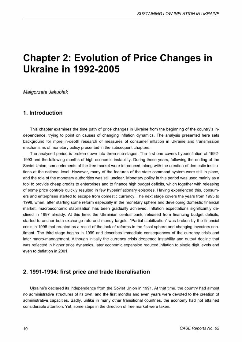
The initial January 1992 liberalisation was forced by the earlier developments in Russia. As prices in Russia were freed on a large scale, there were no economic borders, and Ukraine had no own currency, the country had to follow its neighbour in order to stop outflow of goods. However, the Ukraine’s reaction had a mixed character, as some factors of indirect price control were introduced (Dabrowski, 1994). Next policy package came in December 1992, following the appointment of the Kuchma government. Although some prices were freed – mainly transport tariffs and refined oil products – the category of regulated prices was broadened. The extent of the first two waves of price liberalisation is presented in Table 1.
Table 1. Price control in 1992-1993
Beginning of 1992 Mid-1993 Type of prices Share in total
wholesale turnover Share in retail
turnover Share in total
wholesale turnover Share in retail
turnover Administered prices 17% 12% 11% 10-12% Regulated prices 57% 67% 30-40% 30-40% “Free” prices 26% 21% 50-60% 48-60% Total 100% 100% 100% 100%
Source: Dabrowski (1994: 7, 9) after IMF (1993: 18) and Swiecicki and Wellisz (1993).
Prices in 1992 increased more than twenty-fold. However, this partial liberalisation did not result in the abundant supply, and the upward pressure on prices continued. It should be mentioned, that this price rises were caused primarily by internal factors – the combination of liberalisation and other domestic policies plus continuing shortage of commodities. In 1992, Russia was still supplying Ukraine’s heavy industry with cheap energy resources.
When looking for the causes of the burst of inflation in 1992, the following explanation emerges. First of all, the liberalisation of prices gave an initial impulse. However, as the liberalisation was incomplete and it was not matched by the adjustment of other policies, pressure on prices continued, as the direct effect of the governments’ strategy (or rather of its lack). Particularly Fokin government (stepped back in autumn 1992) presented strong reservation to market-oriented reforms, and tried to preserve as many from the former eco-nomic system as possible (Dabrowski, 1994). But even the next Kuchma government, formed also from some representatives of democratic opposition, was heavily constrained by industrial lobbies. The “soft” macroeconomic policies had a component of liquidity injection into the economy. As a result of industrial lob-bying pressure, off-budget subsidies and directed credits to enterprises amounted to around 16% of GDP (Kravchuk, 1998: 14). According to research of Babanin (1994, after Kravchuk, 1998), credits to enterprises were the primary source of the 1992 to mid-1993 price surge. Moreover, it was found that besides that many enterprises – particularly those supplying non-food consumer goods – were almost free to set market-clearing prices for their output, they nevertheless chose to maintain excess demand for their goods (Sunda-kov et al., 1994) and see prices for their products rising.
2.2. 1993-1994: hyperinflation and shortly after The period from 1993 to early 1995 was characterised by the gradual moves backwards from the high
state control of the setting up prices, granting huge subsidies to enterprises and financing budget deficits
3 Weighted by their share in retail trade (after Polomski, K., 1996).
SUSTAINING LOW INFLATION IN UKRAINE
CASE Reports No. 62 12
through money emission. These moves were often accommodative, and forced either by the external situa-tion or by emerging domestic market.
There were not many attempts toward relaxing price controls in 1993-1994. Actually, the first half of 1993 saw even an increase of state interventions into the setting up prices. At the beginning of 1993, many agri-cultural procurement prices were indexed to the basket of inputs, which created permanent inflationary pres-sure (Dabrowski, 1994). Couple of months later, in early 1993, despite the hyperinflation mounting by over 20 percent month by month, the influential Ukraine’s Trade Unions Federation managed to hamper expected administrative price raises. The government was still intervening by setting the maximal level of mark-up on prices (55% of producer’s price, 25% on first-need commodities), and controlling pricing of enterprises classi-fied as monopolies.
There were no serious attempts towards price liberalisation further in 1994. The government was only trying to make some adjustment of prices. However, the October 1994 decree on “setting prices in the condi-tions of market reforms” removed some earlier limits on the mark-ups on prices of consumer goods (Polom-ski, 1996).
There were some further rises in the prices of services regulated by the state during the first half of 1995. And, as declared by the Ministry of Economy in mid-1995, regulated prices covered only 5% of enterprises and 10% of the retail trade. However, the prices for rents and other communal services for households cov-ered only 30% of their costs; the tariffs for electrical energy were at the level of 80%, while the prices for natural gas oscillated around 30% of its costs of production. In mid-1995, it was expected that tariffs for city transport would cover 50% of its cost. In addition, a substantial part of the Ukrainian population continued to benefit from discounted tariffs.
The existence of controlled prices was only the “cover” part of the story. The preservation of such high state control of the domestic market was caused by the fact that industrial lobbies wanted to see prices for their production controlled, thus prolonging the duration of central planning, and receive subsidies. This situation made them feel very comfortable, the enterprises did not need to react to the changing market con-ditions; there was only the need to adhere to the system of state commands. Such continuous existence of strong lobbies, opposing to any changes, was possible due to the very limited progress in privatisation. State still owned all the large production plants. Only small retail shops and outlets had private owners.
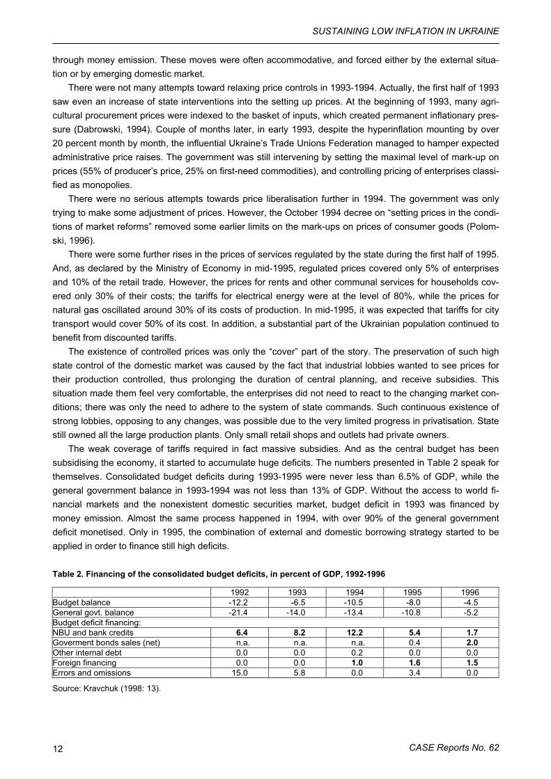
The weak coverage of tariffs required in fact massive subsidies. And as the central budget has been subsidising the economy, it started to accumulate huge deficits. The numbers presented in Table 2 speak for themselves. Consolidated budget deficits during 1993-1995 were never less than 6.5% of GDP, while the general government balance in 1993-1994 was not less than 13% of GDP. Without the access to world fi-nancial markets and the nonexistent domestic securities market, budget deficit in 1993 was financed by money emission. Almost the same process happened in 1994, with over 90% of the general government deficit monetised. Only in 1995, the combination of external and domestic borrowing strategy started to be applied in order to finance still high deficits.
Table 2. Financing of the consolidated budget deficits, in percent of GDP, 1992-1996
1992 1993 1994 1995 1996 Budget balance -12.2 -6.5 -10.5 -8.0 -4.5 General govt. balance -21.4 -14.0 -13.4 -10.8 -5.2 Budget deficit financing: NBU and bank credits 6.4 8.2 12.2 5.4 1.7 Goverment bonds sales (net) n.a. n.a. n.a. 0.4 2.0 Other internal debt 0.0 0.0 0.2 0.0 0.0 Foreign financing 0.0 0.0 1.0 1.6 1.5 Errors and omissions 15.0 5.8 0.0 3.4 0.0
Source: Kravchuk (1998: 13).
Hryvniv V., Jakubiak M., Mykhaylychenko M., Novoseletska O., Paczynski W., Wozniak P.
CASE Reports No. 63 13
Financing budget deficits through the money emission was not the only source of monetary expansion. The other source was the policy of extending cheap credit to industrial and agricultural enterprises. This was done along with the view that economy had to be stabilised by supporting production. According to Dabrowski (1994:19), the strongest pressure on the monetary authority to soften its policy during 1992-1994 was being exerted by the Ukrainian MPs and trade unions, which – with passive reaction of the NBU – played de facto the role of Ukraine’s monetary authorities. Off-budgetary credits to enterprises were in reality the subsidies – first of all, real interest rates were negative, and what more, the probability of repayment of large part of these credits was low. The growth of the banking system credit to public enterprises in 1993 (14 times in one year) was even outpacing the growth of credit to the government (which grew two times in 1992-1993).
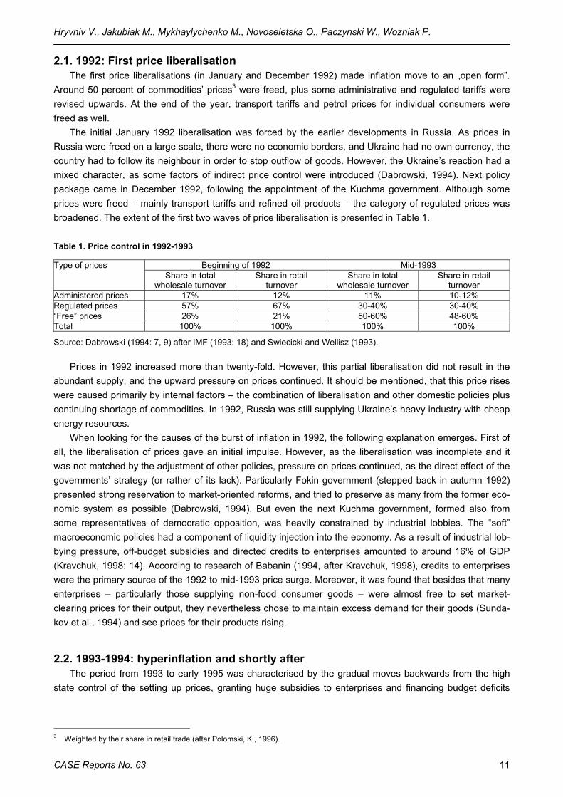
The continuous monetary expansion coupled with the attempts to preserve the command system of pro-duction, and accommodative increases of controlled prices led inevitably to the acceleration in the rates of inflation. Only in 1993 there were five hyperinflationary episodes, with consumer prices rising over 50% per month (see Table 3). The late 1992 price adjustments and December 1992 price liberalisation contributed to over 70% inflation in January, and to the nearly 30% CPI rise during the following month (Dabrowski, 1994). The next three months saw lower (although still high; over 20%) inflation, as there was temporary tightening of fiscal policies (no need to monetise budget deficit), and better supply of consumer products. However, CPI rose again by over 70% monthly in June 1993, and the hyperinflationary spiral burst in September 1993. Prices rose over 90% in December 1993 per month, and for the whole year 1993, they increased over one hundred times. The first signs of stabilisation came in 1994, as the monthly inflation rates came to the one digit levels. However, following another wave of monetising deficit of the general government of the summer months in 1994, at a verge of stabilisation, monthly inflation in November 1994 reached again over 70%.
Table 3. Consumer price inflation, monthly changes, 1992-1996
1992 1993 1994 1995 1996 January 252.4 73.2 19.2 21.2 9.4 February 15.3 28.8 12.6 18.1 7.4 March 12.1 22.1 5.7 11.4 3.0 April 7.6 23.6 6.0 5.8 2.4 May 14.4 27.6 5.2 4.6 0.7 June 26.5 71.7 3.9 4.8 0.1 July 22.1 37.6 2.1 5.2 0.2 August 8.3 21.7 2.6 4.6 5.7 September 10.6 80.3 7.3 14.2 2.0 October 12.4 66.1 22.6 9.1 1.5 November 22.0 45.3 72.3 6.2 1.2 December 35.1 90.8 28.4 4.6 0.9 End-year inflation 1821.7 10155.0 401.1 181.7 39.9
Source: IFS IMF and Dabrowski (1994: 22; data for January 1992).
The findings of the research by Lissovolik (2003) – on the determinants of inflation in Ukraine – revealed that the broad money was indeed cointegrated with the CPI for 1993-1995. This means that weak monetary policy has been the primary cause of the hyperinflation of 1993-1995. The same conclusion is achieved by de Menil (1996), who notes that, in particular, the 1992 monetary expansion increased the pressure on prices and stood behind the hyperinflation of 1993. Then later, increase in credits for the agricultural sector in summer 1994 caused the acceleration in the rate of inflation a couple of months later. De Menil also underlined the im-portance of inflation expectations in Ukraine, particularly the rise in these expectations following administered price increases. Kravchuk (1998) examined what where the roots for the 1992-1996 inflation, treating the growth of money supply as the intermediary cause. He showed that the main factor aggravating inflation in Ukraine at this time were the large quantities of cheap credit extended to the enterprise sector.
Finally, one more topic important for the 1993-1994 price rises should be mentioned. This is the reaction of the general public and the shrinkage of the demand for money. The year 1993 differed from the previous
SUSTAINING LOW INFLATION IN UKRAINE
CASE Reports No. 62 14
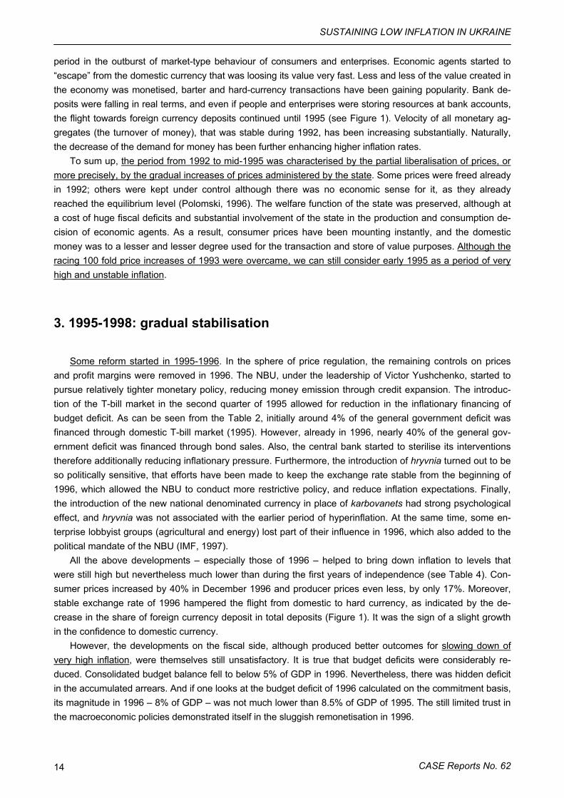
period in the outburst of market-type behaviour of consumers and enterprises. Economic agents started to “escape” from the domestic currency that was loosing its value very fast. Less and less of the value created in the economy was monetised, barter and hard-currency transactions have been gaining popularity. Bank de-posits were falling in real terms, and even if people and enterprises were storing resources at bank accounts, the flight towards foreign currency deposits continued until 1995 (see Figure 1). Velocity of all monetary ag-gregates (the turnover of money), that was stable during 1992, has been increasing substantially. Naturally, the decrease of the demand for money has been further enhancing higher inflation rates.
To sum up, the period from 1992 to mid-1995 was characterised by the partial liberalisation of prices, or more precisely, by the gradual increases of prices administered by the state. Some prices were freed already in 1992; others were kept under control although there was no economic sense for it, as they already reached the equilibrium level (Polomski, 1996). The welfare function of the state was preserved, although at a cost of huge fiscal deficits and substantial involvement of the state in the production and consumption de-cision of economic agents. As a result, consumer prices have been mounting instantly, and the domestic money was to a lesser and lesser degree used for the transaction and store of value purposes. Although the racing 100 fold price increases of 1993 were overcame, we can still consider early 1995 as a period of very high and unstable inflation.
3. 1995-1998: gradual stabilisation
Some reform started in 1995-1996. In the sphere of price regulation, the remaining controls on prices and profit margins were removed in 1996. The NBU, under the leadership of Victor Yushchenko, started to pursue relatively tighter monetary policy, reducing money emission through credit expansion. The introduc-tion of the T-bill market in the second quarter of 1995 allowed for reduction in the inflationary financing of budget deficit. As can be seen from the Table 2, initially around 4% of the general government deficit was financed through domestic T-bill market (1995). However, already in 1996, nearly 40% of the general gov-ernment deficit was financed through bond sales. Also, the central bank started to sterilise its interventions therefore additionally reducing inflationary pressure. Furthermore, the introduction of hryvnia turned out to be so politically sensitive, that efforts have been made to keep the exchange rate stable from the beginning of 1996, which allowed the NBU to conduct more restrictive policy, and reduce inflation expectations. Finally, the introduction of the new national denominated currency in place of karbovanets had strong psychological effect, and hryvnia was not associated with the earlier period of hyperinflation. At the same time, some en-terprise lobbyist groups (agricultural and energy) lost part of their influence in 1996, which also added to the political mandate of the NBU (IMF, 1997).
All the above developments – especially those of 1996 – helped to bring down inflation to levels that were still high but nevertheless much lower than during the first years of independence (see Table 4). Con-sumer prices increased by 40% in December 1996 and producer prices even less, by only 17%. Moreover, stable exchange rate of 1996 hampered the flight from domestic to hard currency, as indicated by the de-crease in the share of foreign currency deposit in total deposits (Figure 1). It was the sign of a slight growth in the confidence to domestic currency.
However, the developments on the fiscal side, although produced better outcomes for slowing down of very high inflation, were themselves still unsatisfactory. It is true that budget deficits were considerably re-duced. Consolidated budget balance fell to below 5% of GDP in 1996. Nevertheless, there was hidden deficit in the accumulated arrears. And if one looks at the budget deficit of 1996 calculated on the commitment basis, its magnitude in 1996 – 8% of GDP – was not much lower than 8.5% of GDP of 1995. The still limited trust in the macroeconomic policies demonstrated itself in the sluggish remonetisation in 1996.
Hryvniv V., Jakubiak M., Mykhaylychenko M., Novoseletska O., Paczynski W., Wozniak P.
CASE Reports No. 63 15
Table 4. Inflation and monetary aggregates in Ukraine in 1992-1996
CPI y/y PPI y/y end-year average end-year average
Monetary base y/y changes
Currency in circulation (M0) y/y changes
Broad money (M2) y/y changes
1992 2000 - - - - 1567 942 1993 10156 4735 9502 4619 1560 2460 1828 1994 401 891 774 1134 407 520 567 1995 182 377 172 489 133 231 113 1996 40 80 17 52 40 54 32
Source: IMF Staff Country Report no. 97/109, IMF IFS and own calculations based on NBU data. Note: numbers are percentage changes.
More careful monetary policy started to significantly reduce inflation expectations in 1997. As the gov-ernment has been able to borrow money through the emission of the treasury bills, and the domestic T-bill market was very active (Ukrainian T-bills were giving a premium over Russian GKOs), the NBU could signifi-cantly decrease the financing of the budget through the money emission and was able to concentrate on re-ducing inflation and on keeping the exchange rate stable. As a result, Ukrainian economy made significant progress towards reducing inflation to 10 percent at the end of 1997, and even to single digits in summer 1998 (IMF, 1999; see Figure 2).
Figure 1. Money demand in Ukraine, 1992-2001
0
10
20
30
40
50
60
1992 1993 1994 1995 1996 1997 1998 1999 2000 2001
broad money (M2)/GDP FX deposits/total bank deposits
%
Source: own calculation on the basis of NBU data (1997-2001).
However, this was also the period when the chances for structural reforms were missed. Lack of political will to reform the economy translated itself into continuously high budget deficits. Softening of budget con-straints, unwillingness to cut expenditures and poor tax collection led to the fiscal deficit of 6.7% in 1997. The accumulation of arrears continued, and this year the deficit on the commitment basis reached nearly 11% of Ukrainian GDP, which was higher than in 1994 (Kovalev, 1999). With the lack of structural reforms, and the change in the investors’ sentiments after the 1997 Asian crisis, that made external borrowing more difficult, the NBU started to “substitute” private investors thus rolling over the existing government obligations. The share of T-bills purchased by the central bank was over 75% of their total stock in September 1997 (Kovalev, 1999). The circumstances limited any financing at acceptable rates; the yields on the T-bills have been grow-ing and their maturity has been plunging. Moreover, there was no reliable plan as how to repay the growing obligations in the future. Some analysts even argue that the “financial pyramid” has been constructed from the beginning of the functioning of the domestic T-bill market.
From 1997, the central bank has been trying to ease pressures on the exchange rate, by intervening on the foreign exchange. However, these actions at a certain point made further sterilisation of money supply impossible (hence created another source of pressures on hryvnia) and with the sudden outflow of short-
SUSTAINING LOW INFLATION IN UKRAINE
CASE Reports No. 62 16
term capital led to the near depletion of the foreign reserves of the NBU. This was how the financial crisis of September 1998 ended the period of “incomplete stability”. In the eve of a currency crash inflation reached record lows, although the NBU has been fighting to lessen the pressures on hryvnia already since October 1997. At least inflation has been temporarily constrained; in 1998 it remained on average below 10 percent.
4. 1998-2005: macroeconomic stabilisation and post-crisis expansion
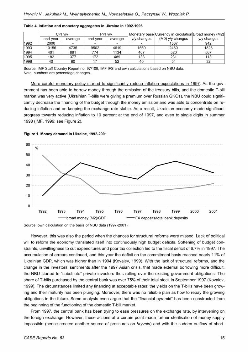
The devaluation of hryvnia in September 1998 stimulated an acceleration of inflationary processes and led to faster price growth in the last quarter of 1998. The currency crisis initiated limited inflationary pass-through in which consumer prices (grew by 20% in December 1998) were initially much less affected than producer prices (grew by 35.4% at the end of 1998). The average annual CPI inflation rate in 1998 was equal to 10.6% which was the lowest level in the period of 1996-2001. The limited inflationary pass-through of hryvnia de-valuation can be explained by restrained growth of money supply and better crisis management than in the case of Russia (see Dabrowski, Gorski and Jarocinski, 1999). Due to the collapse of the government bond market (foreign capital outflow), the reduction of state subsidies and the absence of crediting of real sector through the money emission, there was no significant increase in the money supply. In 1998, annual growth rates of monetary aggregates were the lowest in the period of 1996-2001 (22% y/y and 25% y/y for a mone-tary base and broad money (M3) respectively). As a result, enterprises had not enough resources to raise wage payments that ultimately led to a reduction in real incomes and lower demand for goods. From this viewpoint, the low demand for goods (as population was impoverished) may be considered as one of the rea-sons for the absence of the significant price increases in 1998 (Dabrowski and Jakubiak ed., 2003). It is also probable that Ukrainians significantly reduced their demand for imported first-need commodities, thus also reducing the pass-through on CPI. Furthermore, housing and utility tariffs that constitute around 18% of con-sumer basket were frozen by the resolution of Verkhovna Rada, hence this channel of monetary transmission was initially limited and spread over time. The devaluation of hryvnia had much stronger effect on producer prices because Ukrainian heavy industry is based on imported energy recourses.
Figure 2. Growth of monetary base and inflation, 1996-1999
020406080
100120140160180
Q1 Q2 Q3 Q4 Q1 Q2 Q3 Q4 Q1 Q2 Q3 Q4 Q1 Q2 Q3 Q4
1996 1997 1998 1999
monetary base growth CPI changes PPI changes
% yoy
Source: own calculations based on NBU data.
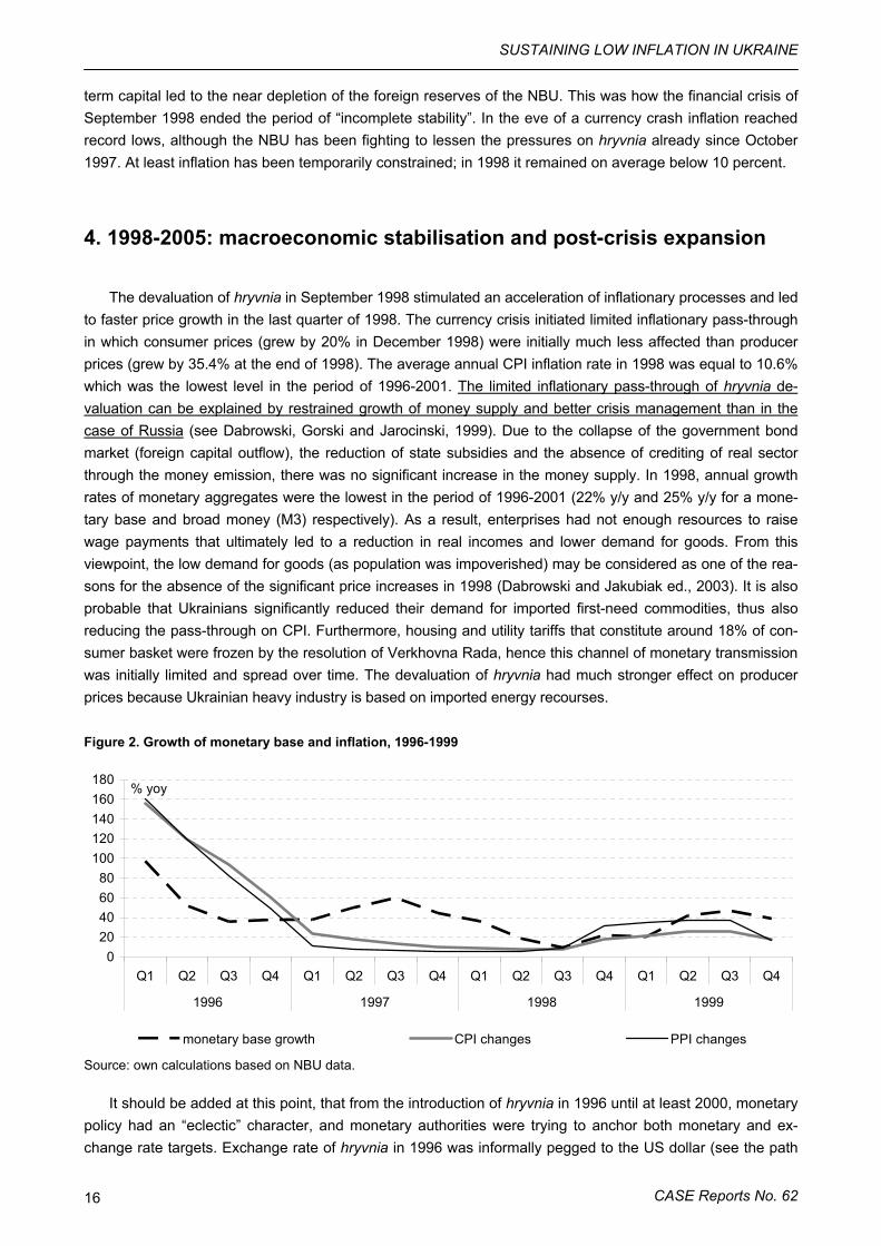
It should be added at this point, that from the introduction of hryvnia in 1996 until at least 2000, monetary policy had an “eclectic” character, and monetary authorities were trying to anchor both monetary and ex-change rate targets. Exchange rate of hryvnia in 1996 was informally pegged to the US dollar (see the path
Hryvniv V., Jakubiak M., Mykhaylychenko M., Novoseletska O., Paczynski W., Wozniak P.
CASE Reports No. 63 17
of HRV/USD in Figure 3), and then in 1997, informal peg was replaced by the formal band of 1.7-1.9 HRV/USD (IMF, 2005). The band has been moved on several occasions, first in January 1998, and then – after the currency crisis hit in early September 1998. This was the time when hryvnia was let to depreciate and lost over 50% in one month. The band has been then readjusted couple of times, and in 1999-2000 ex-change rate was more or less flexible. Starting from 2000, heavy interventions on the foreign exchange re-vealed that the central bank started to fix again the currency, and from 2001 until early 2005 the exchange rate has been the nominal anchor of the monetary policy. Ukraine then followed a hard peg to the US dollar (see Figure 3), notwithstanding strong appreciation pressures, and weak results in fighting inflation starting from 2004. The currency has been allowed to appreciate in Spring 2005 only.
The adherence to exchange rate as a nominal anchor is defined in the Constitution of Ukraine, adopted in 1996. According to the Constitution, the principal role of the central bank is to maintain the stability of the national currency. For this purpose the bank is also responsible for supporting stable banking system, and ensure the stability of prices4.
Figure 3. Nominal exchange rates of hryvnia to ECU/EUR and USD, 1996-2005
1
2
3
4
5
6
7
8
Jan-
96
Jun-
96
Nov
-96
Apr
-97
Sep
-97
Feb-
98
Jul-9
8
Dec
-98
May
-99
Oct
-99
Mar
-00
Aug
-00
Jan-
01
Jun-
01
Nov
-01
Apr
-02
Sep
-02
Feb-
03
Jul-0
3
Dec
-03
May
-04
Oct
-04
Mar
-05
UAH/USD UAH/EUR
Source: NBU.
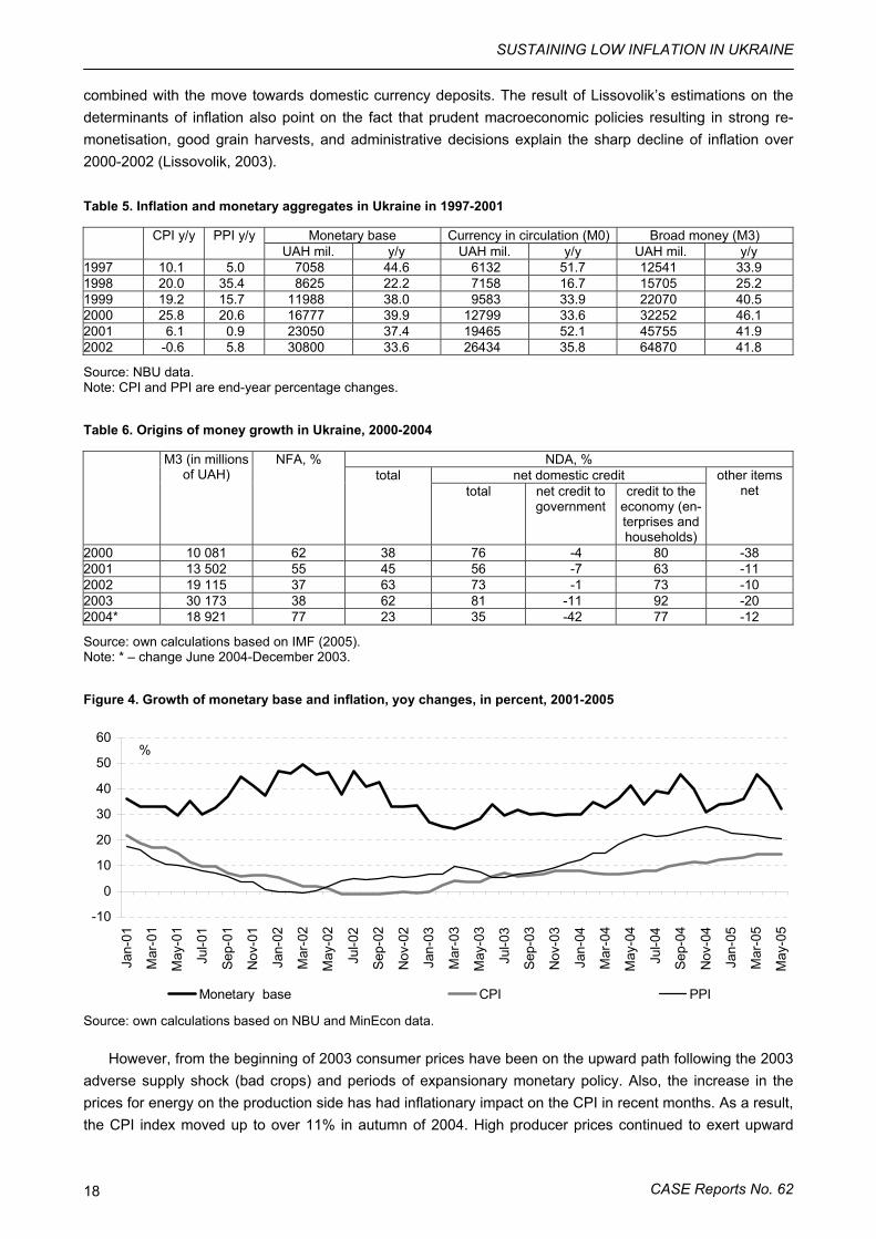
Coming back to months following the currency crisis, contrary to the careful and restrictive monetary pol-icy of 1998, the NBU turned to the monetary expansion in the following year (see Table 5). The “cheap money” policy continued for another 3 years. As we can see from Table 6, increase in credit to the domestic non-financial sector have played the leading role in money creation since 2000. And these were mainly cred-its to enterprises. However, notwithstanding persistent monetary expansion in 1999-2001, inflation started to diminish already in 2001.
Low inflation recorded by the end of 2001 (6 percent on the annual basis in December 2001) and even the deflation of 2002 can be attributable to the increase in the demand for money. The trust of economic agents and society into national currency and macroeconomic policies increased visibly in 2001, thus allow-ing for the accommodation of the expansionary monetary policy of 2001 and early 2002 without the pass-through on inflation. The low inflation, and even the deflation of 2002, was possible also due to the supply shock – good weather conditions and abundant supply of agricultural products made prices for food fall. The National Bank of Ukraine had therefore luck – sharp, unexpected rise in demand for money combined with the supply-side shock helped in disinflation, although the NBU has been extending credit on a large scale. The situation is depicted on Figure 4, where the growing money supply of 2002 is combined with disinflation. Strengthening money demand during 2000-2001 can be observed on Figure 1, where higher monetisation is
4 For further discussion of the central bank policies see chapter by Novoseletska in this volume.
SUSTAINING LOW INFLATION IN UKRAINE
CASE Reports No. 62 18
combined with the move towards domestic currency deposits. The result of Lissovolik’s estimations on the determinants of inflation also point on the fact that prudent macroeconomic policies resulting in strong re-monetisation, good grain harvests, and administrative decisions explain the sharp decline of inflation over 2000-2002 (Lissovolik, 2003).
Table 5. Inflation and monetary aggregates in Ukraine in 1997-2001
Monetary base Currency in circulation (M0) Broad money (M3) CPI y/y PPI y/y UAH mil. y/y UAH mil. y/y UAH mil. y/y
1997 10.1 5.0 7058 44.6 6132 51.7 12541 33.9 1998 20.0 35.4 8625 22.2 7158 16.7 15705 25.2 1999 19.2 15.7 11988 38.0 9583 33.9 22070 40.5 2000 25.8 20.6 16777 39.9 12799 33.6 32252 46.1 2001 6.1 0.9 23050 37.4 19465 52.1 45755 41.9 2002 -0.6 5.8 30800 33.6 26434 35.8 64870 41.8
Source: NBU data. Note: CPI and PPI are end-year percentage changes.
Table 6. Origins of money growth in Ukraine, 2000-2004
NDA, % net domestic credit
M3 (in millions of UAH)
NFA, % total
total net credit to government
credit to the economy (en-terprises and households)
other items net
2000 10 081 62 38 76 -4 80 -38 2001 13 502 55 45 56 -7 63 -11 2002 19 115 37 63 73 -1 73 -10 2003 30 173 38 62 81 -11 92 -20 2004* 18 921 77 23 35 -42 77 -12
Source: own calculations based on IMF (2005). Note: * – change June 2004-December 2003.
Figure 4. Growth of monetary base and inflation, yoy changes, in percent, 2001-2005
-10
0
10
20
30
40
50
60
Jan-
01
Mar
-01
May
-01
Jul-0
1
Sep-
01
Nov
-01
Jan-
02
Mar
-02
May
-02
Jul-0
2
Sep-
02
Nov
-02
Jan-
03
Mar
-03
May
-03
Jul-0
3
Sep-
03
Nov
-03
Jan-
04
Mar
-04
May
-04
Jul-0
4
Sep-
04
Nov
-04
Jan-
05
Mar
-05
May
-05
Monetary base CPI PPI
%
Source: own calculations based on NBU and MinEcon data.
However, from the beginning of 2003 consumer prices have been on the upward path following the 2003 adverse supply shock (bad crops) and periods of expansionary monetary policy. Also, the increase in the prices for energy on the production side has had inflationary impact on the CPI in recent months. As a result, the CPI index moved up to over 11% in autumn of 2004. High producer prices continued to exert upward
Hryvniv V., Jakubiak M., Mykhaylychenko M., Novoseletska O., Paczynski W., Wozniak P.
CASE Reports No. 63 19
pressure on consumer prices in following months. The political crisis and banking sector instability that be-came apparent in end-2004 probably added to inflation expectations. Therefore, inflation is expected to re-main above 10% in 2005. The current instability of inflation reminds the period of high and volatile rates of 1992-1996, and can constrain the growth of demand for money thus hampering further re-monetisation.
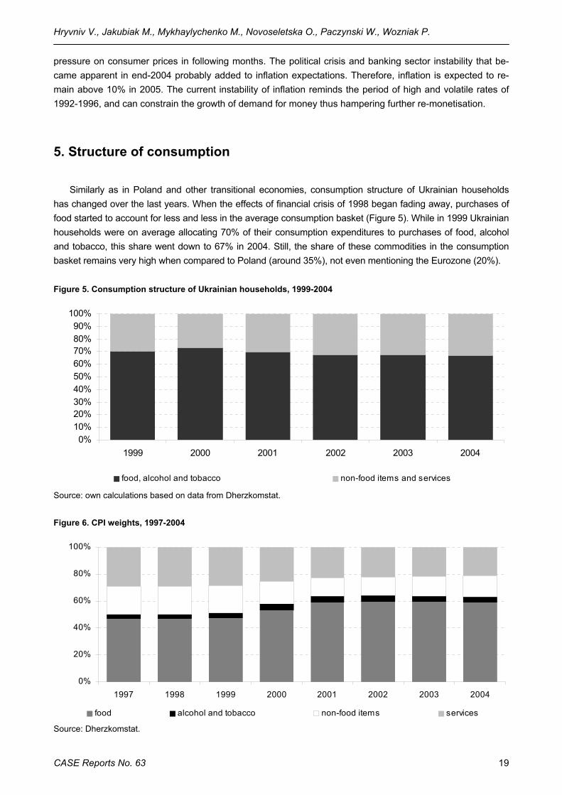
5. Structure of consumption
Similarly as in Poland and other transitional economies, consumption structure of Ukrainian households has changed over the last years. When the effects of financial crisis of 1998 began fading away, purchases of food started to account for less and less in the average consumption basket (Figure 5). While in 1999 Ukrainian households were on average allocating 70% of their consumption expenditures to purchases of food, alcohol and tobacco, this share went down to 67% in 2004. Still, the share of these commodities in the consumption basket remains very high when compared to Poland (around 35%), not even mentioning the Eurozone (20%).
Figure 5. Consumption structure of Ukrainian households, 1999-2004
0%10%20%30%40%50%60%70%80%90%
100%
1999 2000 2001 2002 2003 2004
food, alcohol and tobacco non-food items and services
Source: own calculations based on data from Dherzkomstat.
Figure 6. CPI weights, 1997-2004
0%
20%
40%
60%
80%
100%
1997 1998 1999 2000 2001 2002 2003 2004
food alcohol and tobacco non-food items services
Source: Dherzkomstat.
SUSTAINING LOW INFLATION IN UKRAINE
CASE Reports No. 62 20
Therefore, it should to be remembered that consumption prices in Ukraine have been more volatile than in more advanced transition economies partly due to the larger proportion of food in consumption basket. This effect was up to 2000 mitigated to some extent by the actual CPI weights used by the statistical office (see Figure 6) that lowered the effect of food prices on the whole CPI. The measured structure of consump-tion and the CPI weights coincide in recent years.
6. Summary
The text presents an overview of dynamics of prices in Ukraine during the last 15 years, pointing on prin-cipal causes of inflation during different periods. The description starts from the early 1990s when, after the breakaway from the Soviet Union, the country had to face changing external environment, which, together with the lack of will to complete the move towards market economy by Ukrainian leaders, resulted in hyperin-flation. Later years of 1996-1998 brought better macro-policies, which helped to reduce inflation. However, this period of relative stability was broken by the financial crisis of 1998. Exchange rate based stabilisation in place since early 2000 introduced together with hardening budget constraints in the real sector facilitated disinflation, remonetisation, and increased trust of the economic agents in government policies in general. However, it seems that together with the opening of Ukraine’s financial market, continuation of exchange-based stabilisation is unsustainable and there are important costs associated with it. One such costs is higher inflation, already observable since mid-2004. The paper also presents the structure of Ukraine’s households consumption basket and shows how it has evolved over the years.
References
Babanin, O. (1994). Inflationary Processes in the Ukrainian Economy. The Ukrainian Legal and Eco-nomic Bulletin, June, pp. 14:21.
Dabrowski, M. (1994). Ukrainian Way to Hyperinflation. CASE Studies and Analyses No. 12. Dabrowski, M. and M. Jakubiak (ed.) (2003). The Sources of Economic Growth in Ukraine after 1998
Currency Crisis and the Country’s Prospects. CASE: Report No. 55. Dekhtiarchuk, M. (1999). Monetary Stabilisation in Ukraine: Difficulties and Results. In: M. Dabrowski
(ed.), M. Dekhtiarchuk, U. Gorski, P. Kovalev, Y. Kuz’min, and K. Sultan, Ukraine: From Fragile Stabilisation to Financial Crisis. CASE Studies and Analyses No. 158.
IMF (2005). Ukraine, IMF Staff Country Report No. 05/21. IMF (1999). Ukraine. IMF Staff Country Report No. 99/42. IMF (1997). Ukraine. IMF Staff Country Report No. 97/109. IMF (1993). Ukraine. Recent Economic Developments. European II Department. 9 June 1993, unpub-
lished memo. Kovalev, P. (1999). Some Fiscal Policy Problems. In: M. Dabrowski (ed.), M. Dekhtiarchuk, U. Gorski, P.
Kovalev, Y. Kuz’min, and K. Sultan, Ukraine: From Fragile Stabilisation to Financial Crisis. CASE Studies and Analyses No. 158.
Kravchuk, R. S. (1998). Budget Deficit, Hyperinflation and Stabilisation in Ukraine: 1992-96. CASE Stud-ies and Analyses No. 125.
Landy, L. (1997). Developing Sound banks in Transitional Economies. Structural Reforms in Ukraine. CASE Studies and Analyses No. 115.
Hryvniv V., Jakubiak M., Mykhaylychenko M., Novoseletska O., Paczynski W., Wozniak P.
CASE Reports No. 63 21
Lissovolik, B. (2003). Determinants of Inflation in a Transition Economy: the Case of Ukraine. IMF Work-ing Paper No. 03/126
De Menil, G. (1996). Budget Deficit versus Inflation during 1992-1995. In: M. Dabrowski and R. Antczak: Ukrainian Way To Market Economy (in Polish). CASE: Warsaw.
Polomski, K. (1996). Price Policy on Ukraine. In: M. Dabrowski and R. Antczak: Ukrainian Way To Mar-ket Economy (in Polish). CASE: Warsaw.
Sundakov, A., Ossowski, R., Lane, T. (1994). Shortage Under Free Prices: the Case of Ukraine in 1992. IMF Working Paper No. 94/10.
Swiecicki, M. and S. Wellisz (1993). The Economy of Ukraine. A Memorandum on Stabilisation and Structural Reform, CASE Studies and Analyses No. 2.
SUSTAINING LOW INFLATION IN UKRAINE
CASE Reports No. 62 22
Chapter 3: Polish Disinflation Experience: 1990-2004
Przemysław Woźniak
1. Introduction
Poland’s disinflation experience represents an interesting case for studying various disinflation strate-gies. Polish monetary authorities used many different stabilization strategies to mixed results, but the overall effect has to be considered positive. Within several months after launching the stabilization program, the near-hyperinflation of early 1990 has been brought under control, albeit single-digit inflation rates were not registered on a consistent basis before 2000. Thus, while the initial stabilization success is unquestionable, many economists view the period of high and moderate inflation that prevailed during most of the 1990s as markedly too long and protracted. Likewise, the recent experience of direct inflation targeting is also ambigu-ous: although inflation has been brought down to satisfactorily low levels, no single short-term inflation target has been met since adopting the strategy in 1999.
This paper divides the 15-year period of Polish disinflation into 3 natural periods: the initial stabilization programs of the early 1990s, the period of controlling money supply with the use of market instruments and finally the period of Direct Inflation Targeting. It has to be mentioned that it is not a trivial task to determine when the initial stabilization efforts have been completed and hence when the second ‘free-market’ episode of the Polish disinflation started. In this paper the author follows Kokoszczynski (2004) in applying the criteria of the use of free market instruments of monetary policy to determine the completion of the initial stabilization period. Consequently the first stabilization period is assumed to finish in 1993. The following period of a largely eclectic monetary policy of controlling the money supply and exchange rate is thus assumed to begin in 1993 and end in 1998 when the Monetary Policy Council officially announced adopting the Direct Inflation Strategy that is in place until present. For each of the three periods the main features of the disinflation strat-egy are described: goals and instruments of the monetary policy as well as the success of the disinflation process. Special focus has been placed on the exchange rate policy that was an important component of the disinflation strategy during the decade of the 1990s.
The last section of the paper includes a brief review of the structure of Polish disinflation and the underly-ing relative prices changes. It also investigates the evolution of the structure of the Polish consumption bas-ket and compares it to the structure of the basket in the Euro-zone.
2. The Initial Stabilization 1990-1992
2.1. The Shock Therapy Poland started its systemic and economic transition in the environment of high macroeconomic imbal-
ances and rapidly rising prices. The process of price liberalization was initiated in late 1980s and intensified in
Hryvniv V., Jakubiak M., Mykhaylychenko M., Novoseletska O., Paczynski W., Wozniak P.
CASE Reports No. 63 23
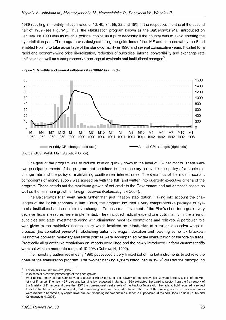
1989 resulting in monthly inflation rates of 10, 40, 34, 55, 22 and 18% in the respective months of the second half of 1989 (see Figure1). Thus, the stabilization program known as the Balcerowicz Plan introduced on January 1st 1990 was as much a political choice as a pure necessity if the country was to avoid entering the hyperinflation path. The program was designed using the guidelines of the IMF and its approval by the Fund enabled Poland to take advantage of the stand-by facility in 1990 and several consecutive years. It called for a rapid and economy-wide price liberalization, reduction of subsidies, internal convertibility and exchange rate unification as well as a comprehensive package of systemic and institutional changes5.
Figure 1. Monthly and annual inflation rates 1989-1992 (in %)
0
10
20
30
40
50
60
70
80
M11989
M41989
M71989
M101989
M11990
M41990
M71990
M101990
M11991
M41991
M71991
M101991
M11992
M41992
M71992
M101992
M11993
0
200
400
600
800
1000
1200
1400
1600
Monthly CPI changes (left axis) Annual CPI changes (right axis)
Source: GUS (Polish Main Statistical Office).
The goal of the program was to reduce inflation quickly down to the level of 1% per month. There were two principal elements of the program that pertained to the monetary policy, i.e. the policy of a stable ex-change rate and the policy of maintaining positive real interest rates. The dynamics of the most important components of money supply was agreed on with the IMF and written into quarterly executive criteria of the program. These criteria set the maximum growth of net credit to the Government and net domestic assets as well as the minimum growth of foreign reserves (Kokoszczynski 2004).
The Balcerowicz Plan went much further than just inflation stabilization. Taking into account the chal-lenges of the Polish economy in late 1980s, the program included a very comprehensive package of sys-temic, institutional and administrative changes. To ensure achievement of the Plan’s short term goals, very decisive fiscal measures were implemented. They included radical expenditure cuts mainly in the area of subsidies and state investments along with eliminating most tax exemptions and relieves. A particular role was given to the restrictive income policy which involved an introduction of a tax on excessive wage in-creases (the so-called popiwek)6, abolishing automatic wage indexation and lowering some tax brackets. Restrictive domestic monetary and fiscal policies were accompanied by the liberalization of the foreign trade. Practically all quantitative restrictions on imports were lifted and the newly introduced uniform customs tariffs were set within a moderate range of 10-20% (Dabrowski, 1992).
The monetary authorities in early 1990 possessed a very limited set of market instruments to achieve the goals of the stabilization program. The two-tier banking system introduced in 19897 created the background 5 For details see Balcerowicz (1997) 6 In excess of a certain percentage of the price growth. 7 Prior to 1989 the National Bank of Poland together with 3 banks and a network of cooperative banks were formally a part of the Min-
istry of Finance. The new NBP Law and banking law accepted in January 1989 extracted the banking sector from the framework of the Ministry of Finance and gave the NBP the conventional central role of the bank of banks with the right to hold required reserved from the banks, set credit limits and grant refinancing credit on the market basis. The rest of the banking sector, i.e. specific banks were meant to become fully commercial and self-financing market entities subject to supervision of the NBP (see Topinski, 1995 and Kokoszczynski, 2004).

SUSTAINING LOW INFLATION IN UKRAINE
CASE Reports No. 62 24
for the development of the financial market but in 1990-1991 one cannot yet speak of a functioning market for securities enabling the central bank carrying out conventional open market operations. Thus the main instruments used by the central bank in early 1990s were setting the interest rates of the refinancing credit, imposing credit ceiling on banks as well as actively using the reserve requirement ratio to control the banks’ liquidity. Figure 2 presents the monthly rates of inflation and domestic money growth as well as the ratio of required reserves and the monthly rate of the refinancing credit.
Figure 2. Monthly Inflation and Domestic M2 Growth and Main Central Bank Instruments in 1990-1992 (refinancing credit interest rate* – percent per month)
05
1015202530354045
M1
1990
M2
1990
M3
1990
M4
1990
M5
1990
M6
1990
M7
1990
M8
1990
M9
1990
M10
199
0M
11 1
990
M12
199
0M
1 19
91M
2 19
91M
3 19
91M
4 19
91M
5 19
91M
6 19
91M
7 19
91M
8 19
91M
9 19
91M
10 1
991
M11
199
1M
12 1
991
M1
1992
M2
1992
M3
1992
M4
1992
M5
1992
M6
1992
M7
1992
M8
1992
M9
1992
M10
199
2M
11 1
992
M12
199
2
%
refinancing credit rate Inflationrequired reserve ratio (for zloty demand deposits) domestic M2 growth
79%
Source: NBP. * The refinancing credit rate was announced on a monthly basis between January and June 1990 and on an annual ba-sis afterwards. Monthly rates for the period July 1990-December 1992 presented in the figure have been calculated using the compound interest formula.
Although some prices were freed in late 1980s, the prices liberalization culminated in January 1990. In this month alone, prices of bread rose by 147%, electrical energy – by 370% while those of furnace fuel, cen-tral heating and hot water – by almost 400%. The effect of these hikes was exacerbated by the fact that the monetary overhang that has been building up during years of shortages and rationing in the form of forced savings, has now made its way to the goods’ market. The resulting aggregate inflation in January was 80% and significantly exceeded the expectations (see Figure 1). Inflation came down quickly from the record high January to 24% in February and to 2-7% in the rest of the year. However the goal of 1% monthly inflation seemed out of reach as the average inflation in the second half of 1990 amounted to 4.4% and 5.7% and 2.4% in the first and second half of 1991.
The goal of the positive interest rate was achieved only partially (see Figure 2). To increase its control over credit in the economy the NBP moved to setting the refinancing rate on a monthly basis in the first half of 1990. Although refinancing rates were set at markedly higher levels than in 1989 (36% and 20% in Janu-ary and February, respectively, compared with 7% in late 1989), the unexpectedly high inflation in January and February resulted in negative refinancing rate in real terms. However, for most remaining months of 1990 the positive real interest was achieved8.
Another key feature of the stabilization program, the fix of the Polish currency, was maintained much longer than originally planned. The exchange rate was officially tied to the USD in January 1990 at the level of 9500 zl/$ with the commitment to keep it there for 3 months, but the arrangement remained in effect for 15
8 The NBP set the refinancing rate on a monthly basis between January and June 1990 to subsequently return to conventional setting
of annual rates. The monthly rates for the period July 1990-December 1992 are thus calculated from the annual rates set by the bank using the usual compounding formula. In view of the consistent disinflation and falling interest rates the rates calculated in this way may thus overstate the actual cost of the refinancing credit in this period.
Hryvniv V., Jakubiak M., Mykhaylychenko M., Novoseletska O., Paczynski W., Wozniak P.
CASE Reports No. 63 25
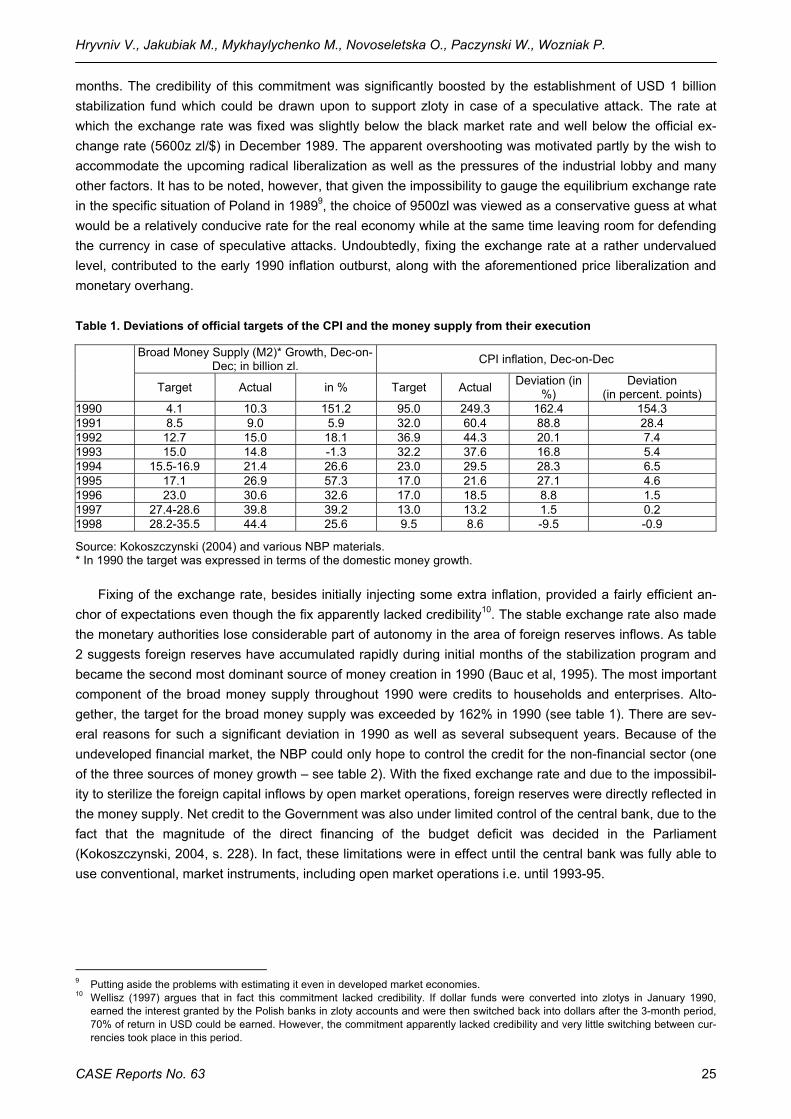
months. The credibility of this commitment was significantly boosted by the establishment of USD 1 billion stabilization fund which could be drawn upon to support zloty in case of a speculative attack. The rate at which the exchange rate was fixed was slightly below the black market rate and well below the official ex-change rate (5600z zl/$) in December 1989. The apparent overshooting was motivated partly by the wish to accommodate the upcoming radical liberalization as well as the pressures of the industrial lobby and many other factors. It has to be noted, however, that given the impossibility to gauge the equilibrium exchange rate in the specific situation of Poland in 19899, the choice of 9500zl was viewed as a conservative guess at what would be a relatively conducive rate for the real economy while at the same time leaving room for defending the currency in case of speculative attacks. Undoubtedly, fixing the exchange rate at a rather undervalued level, contributed to the early 1990 inflation outburst, along with the aforementioned price liberalization and monetary overhang.
Table 1. Deviations of official targets of the CPI and the money supply from their execution
Broad Money Supply (M2)* Growth, Dec-on-Dec; in billion zl. CPI inflation, Dec-on-Dec
Target Actual in % Target Actual Deviation (in %)
Deviation (in percent. points)
1990 4.1 10.3 151.2 95.0 249.3 162.4 154.3 1991 8.5 9.0 5.9 32.0 60.4 88.8 28.4 1992 12.7 15.0 18.1 36.9 44.3 20.1 7.4 1993 15.0 14.8 -1.3 32.2 37.6 16.8 5.4 1994 15.5-16.9 21.4 26.6 23.0 29.5 28.3 6.5 1995 17.1 26.9 57.3 17.0 21.6 27.1 4.6 1996 23.0 30.6 32.6 17.0 18.5 8.8 1.5 1997 27.4-28.6 39.8 39.2 13.0 13.2 1.5 0.2 1998 28.2-35.5 44.4 25.6 9.5 8.6 -9.5 -0.9
Source: Kokoszczynski (2004) and various NBP materials. * In 1990 the target was expressed in terms of the domestic money growth.
Fixing of the exchange rate, besides initially injecting some extra inflation, provided a fairly efficient an-chor of expectations even though the fix apparently lacked credibility10. The stable exchange rate also made the monetary authorities lose considerable part of autonomy in the area of foreign reserves inflows. As table 2 suggests foreign reserves have accumulated rapidly during initial months of the stabilization program and became the second most dominant source of money creation in 1990 (Bauc et al, 1995). The most important component of the broad money supply throughout 1990 were credits to households and enterprises. Alto-gether, the target for the broad money supply was exceeded by 162% in 1990 (see table 1). There are sev-eral reasons for such a significant deviation in 1990 as well as several subsequent years. Because of the undeveloped financial market, the NBP could only hope to control the credit for the non-financial sector (one of the three sources of money growth – see table 2). With the fixed exchange rate and due to the impossibil-ity to sterilize the foreign capital inflows by open market operations, foreign reserves were directly reflected in the money supply. Net credit to the Government was also under limited control of the central bank, due to the fact that the magnitude of the direct financing of the budget deficit was decided in the Parliament (Kokoszczynski, 2004, s. 228). In fact, these limitations were in effect until the central bank was fully able to use conventional, market instruments, including open market operations i.e. until 1993-95.
9 Putting aside the problems with estimating it even in developed market economies. 10 Wellisz (1997) argues that in fact this commitment lacked credibility. If dollar funds were converted into zlotys in January 1990,
earned the interest granted by the Polish banks in zloty accounts and were then switched back into dollars after the 3-month period, 70% of return in USD could be earned. However, the commitment apparently lacked credibility and very little switching between cur-rencies took place in this period.

SUSTAINING LOW INFLATION IN UKRAINE
CASE Reports No. 62 26
2.2. “Second Stabilization”: mid-1990 – 1992 After the initial success of the shock therapy evidenced in a radical fall of inflation in the first quarter of
1990, the restrictive macroeconomic policies began to loosen mostly in reaction to the severe recession in the real sector. Interest rates were radically decreased: the monthly refinancing rate set at 36%, 20% and 10% in the months of the first quarter, respectively, was lowered to 4% in June and 2.5% in July 1990. This triggered a dynamic credit rise in the economy in the economy (see table 2) which coupled with a fast growth of foreign reserves led to a sizeable expansion of money supply in the second and third quarter of 1990. In parallel, sev-eral important components of the restrictive income policy were softened as well (Dabrowski, 1992).
Table 2. Origins of money creation 1990-1996
Net domestic assets, due from Net domestic credit
M2 Net foreign assets Total
Total Households Enterprises Net General
Govern. Debt
A B C D E F H mil. zloty % % % % % % 1990 11670.1 47.8 -11.3 NA NA 63.5 11670.1 1991 9035.3 -2.4 37.1 NA NA 65.3 9035.3 1992 15009.7 25.9 25.8 2.3 23.5 48.3 15009.7 1993 14815.5 17.5 35.4 4.5 30.9 47.1 14815.5 1994 21377.5 32.9 29.9 3.9 26 37.2 21377.5 1995 26952.8 58.7 37.9 5.9 31.9 3.7 26952.8 1996 30541.3 29.9 57.3 14.6 41.4 12.8 30541.3
Source: NBP.
Without the expected effects in the real sector, the loosening of the stabilization package brought rising in-flation (beginning in September) and a worsening in the balance of payments. The macroeconomic situation called for a new stabilization program which was introduced in late 1990. This time the program focused primar-ily on monetary measures. The reserve requirement ratio was raised substantially in July 1990. The rate of the refinancing credit was increased several times: from 34% in July 1990 to 72% in February 1991 on an annual basis. To augment these changes, restrictive credit policy (credit ceilings) was pursed (Topinski 1995).
Figure 3. Real Effective Exchange Rate of the Zloty (1995=100)
30
50
70
90
110
130
150
M1
1989
M1
1990
M1
1991
M1
1992
M1
1993
M1
1994
M1
1995
M1
1996
M1
1997
M1
1998
M1
1999
M1
2000
M1
2001
M1
2002
M1
2003
M1
2004
Source: International Financial Statistics. Note: Increase points to appreciation.
The money supply growth was reduced significantly in 4Q90 and 1Q91 (see table 2). However, the prof-itability of enterprises started to deteriorate rapidly and recessionary tendencies set in again. Additionally the currency fix coupled with high inflation caused dramatic real appreciation (see Figure 3) which was gradually
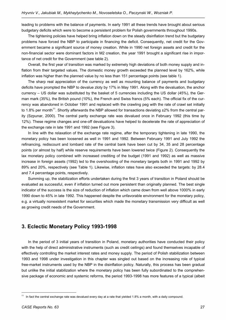
Hryvniv V., Jakubiak M., Mykhaylychenko M., Novoseletska O., Paczynski W., Wozniak P.
CASE Reports No. 63 27
leading to problems with the balance of payments. In early 1991 all these trends have brought about serious budgetary deficits which were to become a persistent problem for Polish governments throughout 1990s.
The tightening policies have helped bring inflation down on the steady disinflation trend but the budgetary problems have forced the NBP to participate in financing the deficit. Consequently, net credit for the Gov-ernment became a significant source of money creation. While in 1990 net foreign assets and credit for the non-financial sector were dominant factors in M2 creation, the year 1991 brought a significant rise in impor-tance of net credit for the Government (see table 2).
Overall, the first year of transition was marked by extremely high deviations of both money supply and in-flation from their targeted values. The domestic money growth exceeded the planned level by 162%, while inflation was higher than the planned value by no less than 151 percentage points (see table 1).
The sharp real appreciation of the currency as well as mounting balance of payments and budgetary deficits have prompted the NBP to devalue zloty by 17% in May 1991. Along with the devaluation, the anchor currency – US dollar was substituted by the basket of 5 currencies including the US dollar (45%), the Ger-man mark (35%), the British pound (10%), the French and Swiss francs (5% each). The official fix of the cur-rency was abandoned in October 1991 and replaced with the crawling peg with the rate of crawl set initially to 1.8% per month11. Shortly afterwards the NBP allowed for transactions deviating ±2% from the central par-ity (Szpunar, 2000). The central parity exchange rate was devalued once in February 1992 (this time by 12%). These regime changes and one-off devaluations have helped to decelerate the rate of appreciation of the exchange rate in late 1991 and 1992 (see Figure 3).
In line with the relaxation of the exchange rate regime, after the temporary tightening in late 1990, the monetary policy has been loosened as well in 1991 and 1992. Between February 1991 and July 1992 the refinancing, rediscount and lombard rate of the central bank have been cut by 34, 35 and 28 percentage points (or almost by half) while reserve requirements have been lowered twice (Figure 2). Consequently the lax monetary policy combined with increased crediting of the budget (1991 and 1992) as well as massive increase in foreign assets (1992) led to the overshooting of the monetary targets both in 1991 and 1992 by 89% and 20%, respectively (see Table 1). Likewise, inflation rates have also exceeded the targets: by 28.4 and 7.4 percentage points, respectively.
Summing up, the stabilization efforts undertaken during the first 3 years of transition in Poland should be evaluated as successful, even if inflation turned out more persistent than originally planned. The best single indicator of the success is the size of reduction of inflation which came down from well above 1000% in early 1990 down to 45% in late 1992. This happened despite the unfavorable environment for the monetary policy, e.g. a virtually nonexistent market for securities which made the monetary transmission very difficult as well as growing credit needs of the Government.
3. Eclectic Monetary Policy 1993-1998
In the period of 3 initial years of transition in Poland, monetary authorities have conducted their policy with the help of direct administrative instruments (such as credit ceilings) and found themselves incapable of effectively controlling the market interest rates and money supply. The period of Polish stabilization between 1993 and 1998 under investigation in this chapter was singled out based on the increasing role of typical free-market instruments used by the NBP in the disinflation policy. Naturally, this process has been gradual but unlike the initial stabilization where the monetary policy has been fully subordinated to the comprehen-sive package of economic and systemic reforms, the period 1993-1998 has more features of a typical (albeit
11 In fact the central exchange rate was devalued every day at a rate that yielded 1.8% a month, with a daily compound.
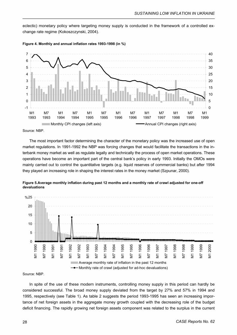
SUSTAINING LOW INFLATION IN UKRAINE
CASE Reports No. 62 28
eclectic) monetary policy where targeting money supply is conducted in the framework of a controlled ex-change rate regime (Kokoszczynski, 2004).
Figure 4. Monthly and annual inflation rates 1993-1998 (in %)
-1
0
1
2
3
4
5
6
7
M11993
M71993
M11994
M71994
M11995
M71995
M11996
M71996
M11997
M71997
M11998
M71998
M11999
0
5
10
15
20
25
30
35
40
Monthly CPI changes (left axis) Annual CPI changes (right axis)
Source: NBP.
The most important factor determining the character of the monetary policy was the increased use of open market regulations. In 1991-1992 the NBP was forcing changes that would facilitate the transactions in the in-terbank money market as well as regulate legally and technically the process of open market operations. These operations have become an important part of the central bank’s policy in early 1993. Initially the OMOs were mainly carried out to control the quantitative targets (e.g. liquid reserves of commercial banks) but after 1994 they played an increasing role in shaping the interest rates in the money market (Szpunar, 2000).
Figure 5.Average monthly inflation during past 12 months and a monthly rate of crawl adjusted for one-off devaluations
0
5
10
15
20
25
M1
1990
M7
1990
M1
1991
M7
1991
M1
1992
M7
1992
M1
1993
M7
1993
M1
1994
M7
1994
M1
1995
M7
1995
M1
1996
M7
1996
M1
1997
M7
1997
M1
1998
M7
1998
M1
1999
M7
1999
M1
2000
%
Average monthly rate of inflation in the past 12 monthsMonthly rate of crawl (adjusted for ad-hoc devaluations)
Source: NBP.
In spite of the use of these modern instruments, controlling money supply in this period can hardly be considered successful. The broad money supply deviated from the target by 27% and 57% in 1994 and 1995, respectively (see Table 1). As table 2 suggests the period 1993-1995 has seen an increasing impor-tance of net foreign assets in the aggregate money growth coupled with the decreasing role of the budget deficit financing. The rapidly growing net foreign assets component was related to the surplus in the current
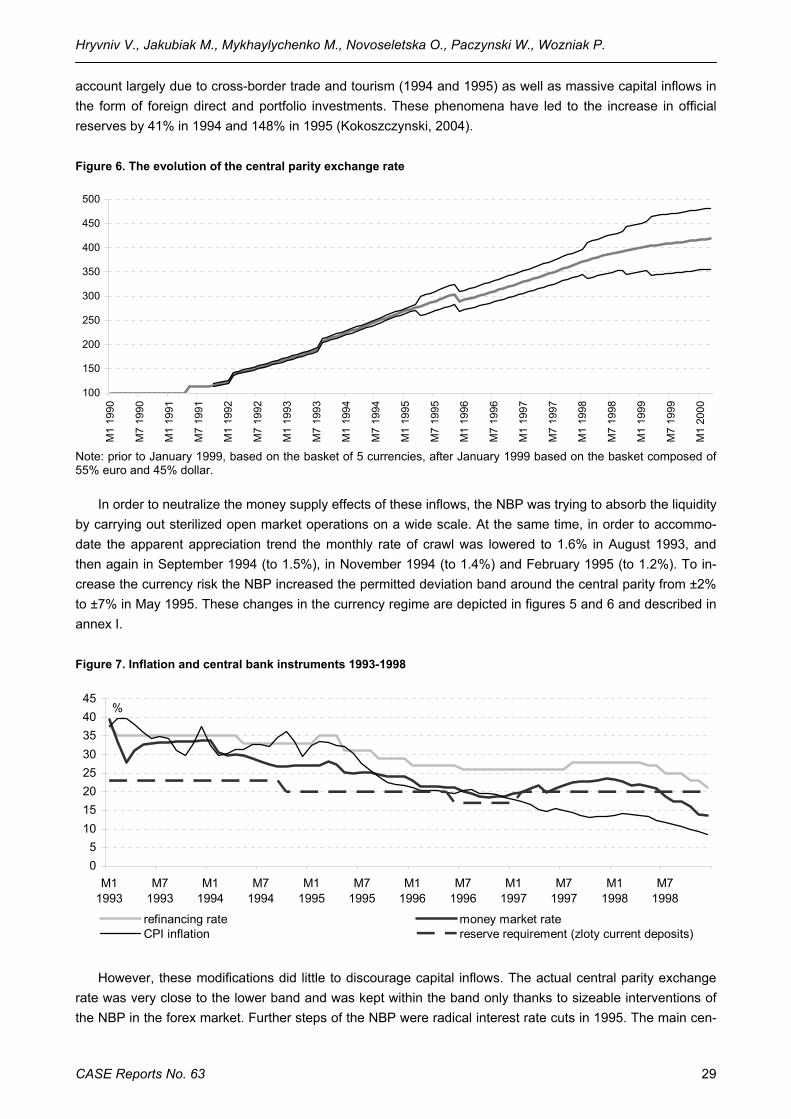
Hryvniv V., Jakubiak M., Mykhaylychenko M., Novoseletska O., Paczynski W., Wozniak P.
CASE Reports No. 63 29
account largely due to cross-border trade and tourism (1994 and 1995) as well as massive capital inflows in the form of foreign direct and portfolio investments. These phenomena have led to the increase in official reserves by 41% in 1994 and 148% in 1995 (Kokoszczynski, 2004).
Figure 6. The evolution of the central parity exchange rate
100
150
200
250
300
350
400
450
500
M1
1990
M7
1990
M1
1991
M7
1991
M1
1992
M7
1992
M1
1993
M7
1993
M1
1994
M7
1994
M1
1995
M7
1995
M1
1996
M7
1996
M1
1997
M7
1997
M1
1998
M7
1998
M1
1999
M7
1999
M1
2000
Note: prior to January 1999, based on the basket of 5 currencies, after January 1999 based on the basket composed of 55% euro and 45% dollar.
In order to neutralize the money supply effects of these inflows, the NBP was trying to absorb the liquidity by carrying out sterilized open market operations on a wide scale. At the same time, in order to accommo-date the apparent appreciation trend the monthly rate of crawl was lowered to 1.6% in August 1993, and then again in September 1994 (to 1.5%), in November 1994 (to 1.4%) and February 1995 (to 1.2%). To in-crease the currency risk the NBP increased the permitted deviation band around the central parity from ±2% to ±7% in May 1995. These changes in the currency regime are depicted in figures 5 and 6 and described in annex I.
Figure 7. Inflation and central bank instruments 1993-1998
05
1015202530354045
M11993
M71993
M11994
M71994
M11995
M71995
M11996
M71996
M11997
M71997
M11998
M71998
%
refinancing rate money market rateCPI inflation reserve requirement (zloty current deposits)
However, these modifications did little to discourage capital inflows. The actual central parity exchange rate was very close to the lower band and was kept within the band only thanks to sizeable interventions of the NBP in the forex market. Further steps of the NBP were radical interest rate cuts in 1995. The main cen-
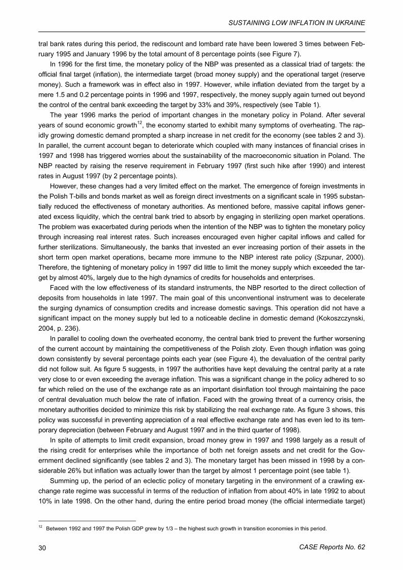
SUSTAINING LOW INFLATION IN UKRAINE
CASE Reports No. 62 30
tral bank rates during this period, the rediscount and lombard rate have been lowered 3 times between Feb-ruary 1995 and January 1996 by the total amount of 8 percentage points (see Figure 7).
In 1996 for the first time, the monetary policy of the NBP was presented as a classical triad of targets: the official final target (inflation), the intermediate target (broad money supply) and the operational target (reserve money). Such a framework was in effect also in 1997. However, while inflation deviated from the target by a mere 1.5 and 0.2 percentage points in 1996 and 1997, respectively, the money supply again turned out beyond the control of the central bank exceeding the target by 33% and 39%, respectively (see Table 1).
The year 1996 marks the period of important changes in the monetary policy in Poland. After several years of sound economic growth12, the economy started to exhibit many symptoms of overheating. The rap-idly growing domestic demand prompted a sharp increase in net credit for the economy (see tables 2 and 3). In parallel, the current account began to deteriorate which coupled with many instances of financial crises in 1997 and 1998 has triggered worries about the sustainability of the macroeconomic situation in Poland. The NBP reacted by raising the reserve requirement in February 1997 (first such hike after 1990) and interest rates in August 1997 (by 2 percentage points).
However, these changes had a very limited effect on the market. The emergence of foreign investments in the Polish T-bills and bonds market as well as foreign direct investments on a significant scale in 1995 substan-tially reduced the effectiveness of monetary authorities. As mentioned before, massive capital inflows gener-ated excess liquidity, which the central bank tried to absorb by engaging in sterilizing open market operations. The problem was exacerbated during periods when the intention of the NBP was to tighten the monetary policy through increasing real interest rates. Such increases encouraged even higher capital inflows and called for further sterilizations. Simultaneously, the banks that invested an ever increasing portion of their assets in the short term open market operations, became more immune to the NBP interest rate policy (Szpunar, 2000). Therefore, the tightening of monetary policy in 1997 did little to limit the money supply which exceeded the tar-get by almost 40%, largely due to the high dynamics of credits for households and enterprises.
Faced with the low effectiveness of its standard instruments, the NBP resorted to the direct collection of deposits from households in late 1997. The main goal of this unconventional instrument was to decelerate the surging dynamics of consumption credits and increase domestic savings. This operation did not have a significant impact on the money supply but led to a noticeable decline in domestic demand (Kokoszczynski, 2004, p. 236).
In parallel to cooling down the overheated economy, the central bank tried to prevent the further worsening of the current account by maintaining the competitiveness of the Polish zloty. Even though inflation was going down consistently by several percentage points each year (see Figure 4), the devaluation of the central parity did not follow suit. As figure 5 suggests, in 1997 the authorities have kept devaluing the central parity at a rate very close to or even exceeding the average inflation. This was a significant change in the policy adhered to so far which relied on the use of the exchange rate as an important disinflation tool through maintaining the pace of central devaluation much below the rate of inflation. Faced with the growing threat of a currency crisis, the monetary authorities decided to minimize this risk by stabilizing the real exchange rate. As figure 3 shows, this policy was successful in preventing appreciation of a real effective exchange rate and has even led to its tem-porary depreciation (between February and August 1997 and in the third quarter of 1998).
In spite of attempts to limit credit expansion, broad money grew in 1997 and 1998 largely as a result of the rising credit for enterprises while the importance of both net foreign assets and net credit for the Gov-ernment declined significantly (see tables 2 and 3). The monetary target has been missed in 1998 by a con-siderable 26% but inflation was actually lower than the target by almost 1 percentage point (see table 1).
Summing up, the period of an eclectic policy of monetary targeting in the environment of a crawling ex-change rate regime was successful in terms of the reduction of inflation from about 40% in late 1992 to about 10% in late 1998. On the other hand, during the entire period broad money (the official intermediate target)
12 Between 1992 and 1997 the Polish GDP grew by 1/3 – the highest such growth in transition economies in this period.
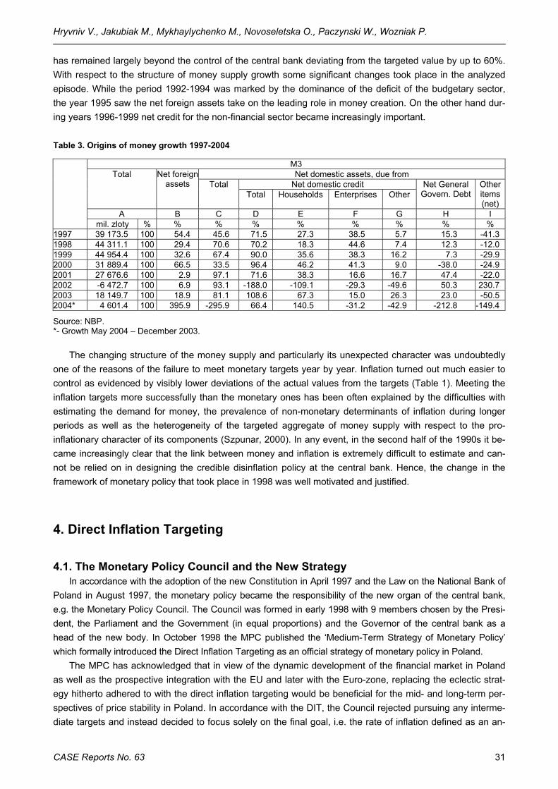
Hryvniv V., Jakubiak M., Mykhaylychenko M., Novoseletska O., Paczynski W., Wozniak P.
CASE Reports No. 63 31
has remained largely beyond the control of the central bank deviating from the targeted value by up to 60%. With respect to the structure of money supply growth some significant changes took place in the analyzed episode. While the period 1992-1994 was marked by the dominance of the deficit of the budgetary sector, the year 1995 saw the net foreign assets take on the leading role in money creation. On the other hand dur-ing years 1996-1999 net credit for the non-financial sector became increasingly important.
Table 3. Origins of money growth 1997-2004
M3 Net domestic assets, due from
Net domestic credit Total Net foreign
assets Total Total Households Enterprises Other
Net General Govern. Debt
Other items (net)
A B C D E F G H I
mil. zloty % % % % % % % % % 1997 39 173.5 100 54.4 45.6 71.5 27.3 38.5 5.7 15.3 -41.3 1998 44 311.1 100 29.4 70.6 70.2 18.3 44.6 7.4 12.3 -12.0 1999 44 954.4 100 32.6 67.4 90.0 35.6 38.3 16.2 7.3 -29.9 2000 31 889.4 100 66.5 33.5 96.4 46.2 41.3 9.0 -38.0 -24.9 2001 27 676.6 100 2.9 97.1 71.6 38.3 16.6 16.7 47.4 -22.0 2002 -6 472.7 100 6.9 93.1 -188.0 -109.1 -29.3 -49.6 50.3 230.7 2003 18 149.7 100 18.9 81.1 108.6 67.3 15.0 26.3 23.0 -50.5 2004* 4 601.4 100 395.9 -295.9 66.4 140.5 -31.2 -42.9 -212.8 -149.4
Source: NBP. *- Growth May 2004 – December 2003.
The changing structure of the money supply and particularly its unexpected character was undoubtedly one of the reasons of the failure to meet monetary targets year by year. Inflation turned out much easier to control as evidenced by visibly lower deviations of the actual values from the targets (Table 1). Meeting the inflation targets more successfully than the monetary ones has been often explained by the difficulties with estimating the demand for money, the prevalence of non-monetary determinants of inflation during longer periods as well as the heterogeneity of the targeted aggregate of money supply with respect to the pro-inflationary character of its components (Szpunar, 2000). In any event, in the second half of the 1990s it be-came increasingly clear that the link between money and inflation is extremely difficult to estimate and can-not be relied on in designing the credible disinflation policy at the central bank. Hence, the change in the framework of monetary policy that took place in 1998 was well motivated and justified.
4. Direct Inflation Targeting
4.1. The Monetary Policy Council and the New Strategy In accordance with the adoption of the new Constitution in April 1997 and the Law on the National Bank of
Poland in August 1997, the monetary policy became the responsibility of the new organ of the central bank, e.g. the Monetary Policy Council. The Council was formed in early 1998 with 9 members chosen by the Presi-dent, the Parliament and the Government (in equal proportions) and the Governor of the central bank as a head of the new body. In October 1998 the MPC published the ‘Medium-Term Strategy of Monetary Policy’ which formally introduced the Direct Inflation Targeting as an official strategy of monetary policy in Poland.
The MPC has acknowledged that in view of the dynamic development of the financial market in Poland as well as the prospective integration with the EU and later with the Euro-zone, replacing the eclectic strat-egy hitherto adhered to with the direct inflation targeting would be beneficial for the mid- and long-term per-spectives of price stability in Poland. In accordance with the DIT, the Council rejected pursuing any interme-diate targets and instead decided to focus solely on the final goal, i.e. the rate of inflation defined as an an-
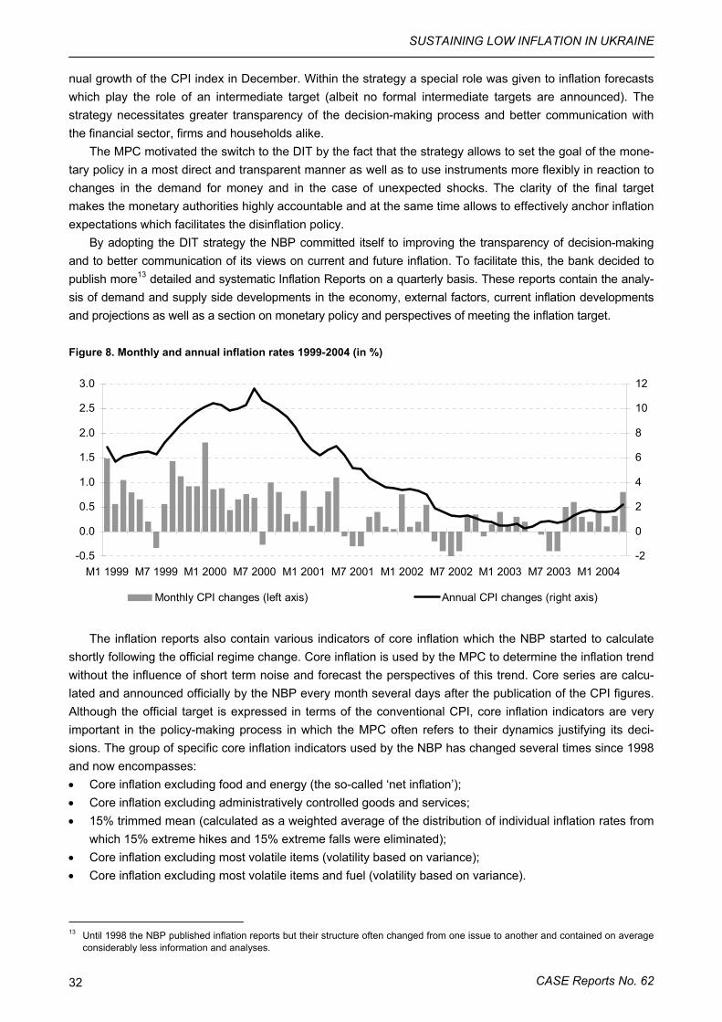
SUSTAINING LOW INFLATION IN UKRAINE
CASE Reports No. 62 32
nual growth of the CPI index in December. Within the strategy a special role was given to inflation forecasts which play the role of an intermediate target (albeit no formal intermediate targets are announced). The strategy necessitates greater transparency of the decision-making process and better communication with the financial sector, firms and households alike.
The MPC motivated the switch to the DIT by the fact that the strategy allows to set the goal of the mone-tary policy in a most direct and transparent manner as well as to use instruments more flexibly in reaction to changes in the demand for money and in the case of unexpected shocks. The clarity of the final target makes the monetary authorities highly accountable and at the same time allows to effectively anchor inflation expectations which facilitates the disinflation policy.
By adopting the DIT strategy the NBP committed itself to improving the transparency of decision-making and to better communication of its views on current and future inflation. To facilitate this, the bank decided to publish more13 detailed and systematic Inflation Reports on a quarterly basis. These reports contain the analy-sis of demand and supply side developments in the economy, external factors, current inflation developments and projections as well as a section on monetary policy and perspectives of meeting the inflation target.
Figure 8. Monthly and annual inflation rates 1999-2004 (in %)
-0.5
0.0
0.5
1.0
1.5
2.0
2.5
3.0
M1 1999 M7 1999 M1 2000 M7 2000 M1 2001 M7 2001 M1 2002 M7 2002 M1 2003 M7 2003 M1 2004-2
0
2
4
6
8
10
12
Monthly CPI changes (left axis) Annual CPI changes (right axis)
The inflation reports also contain various indicators of core inflation which the NBP started to calculate shortly following the official regime change. Core inflation is used by the MPC to determine the inflation trend without the influence of short term noise and forecast the perspectives of this trend. Core series are calcu-lated and announced officially by the NBP every month several days after the publication of the CPI figures. Although the official target is expressed in terms of the conventional CPI, core inflation indicators are very important in the policy-making process in which the MPC often refers to their dynamics justifying its deci-sions. The group of specific core inflation indicators used by the NBP has changed several times since 1998 and now encompasses: • Core inflation excluding food and energy (the so-called ‘net inflation’); • Core inflation excluding administratively controlled goods and services; • 15% trimmed mean (calculated as a weighted average of the distribution of individual inflation rates from
which 15% extreme hikes and 15% extreme falls were eliminated); • Core inflation excluding most volatile items (volatility based on variance); • Core inflation excluding most volatile items and fuel (volatility based on variance).
13 Until 1998 the NBP published inflation reports but their structure often changed from one issue to another and contained on average
considerably less information and analyses.
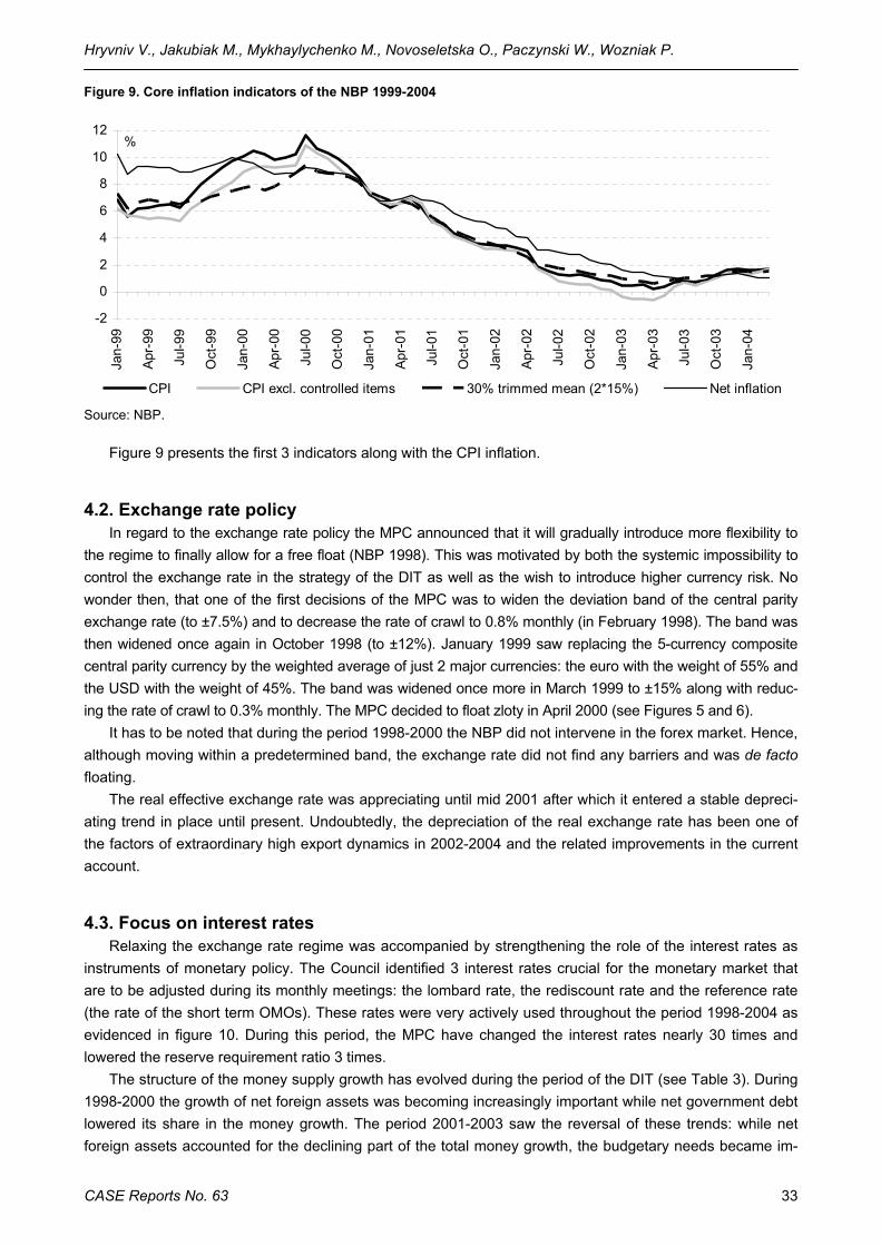
Hryvniv V., Jakubiak M., Mykhaylychenko M., Novoseletska O., Paczynski W., Wozniak P.
CASE Reports No. 63 33
Figure 9. Core inflation indicators of the NBP 1999-2004
-2
0
2
4
6
8
10
12Ja
n-99
Apr-
99
Jul-9
9
Oct
-99
Jan-
00
Apr-
00
Jul-0
0
Oct
-00
Jan-
01
Apr-
01
Jul-0
1
Oct
-01
Jan-
02
Apr-
02
Jul-0
2
Oct
-02
Jan-
03
Apr-
03
Jul-0
3
Oct
-03
Jan-
04
CPI CPI excl. controlled items 30% trimmed mean (2*15%) Net inflation
%
Source: NBP.
Figure 9 presents the first 3 indicators along with the CPI inflation.
4.2. Exchange rate policy In regard to the exchange rate policy the MPC announced that it will gradually introduce more flexibility to
the regime to finally allow for a free float (NBP 1998). This was motivated by both the systemic impossibility to control the exchange rate in the strategy of the DIT as well as the wish to introduce higher currency risk. No wonder then, that one of the first decisions of the MPC was to widen the deviation band of the central parity exchange rate (to ±7.5%) and to decrease the rate of crawl to 0.8% monthly (in February 1998). The band was then widened once again in October 1998 (to ±12%). January 1999 saw replacing the 5-currency composite central parity currency by the weighted average of just 2 major currencies: the euro with the weight of 55% and the USD with the weight of 45%. The band was widened once more in March 1999 to ±15% along with reduc-ing the rate of crawl to 0.3% monthly. The MPC decided to float zloty in April 2000 (see Figures 5 and 6).
It has to be noted that during the period 1998-2000 the NBP did not intervene in the forex market. Hence, although moving within a predetermined band, the exchange rate did not find any barriers and was de facto floating.
The real effective exchange rate was appreciating until mid 2001 after which it entered a stable depreci-ating trend in place until present. Undoubtedly, the depreciation of the real exchange rate has been one of the factors of extraordinary high export dynamics in 2002-2004 and the related improvements in the current account.
4.3. Focus on interest rates Relaxing the exchange rate regime was accompanied by strengthening the role of the interest rates as
instruments of monetary policy. The Council identified 3 interest rates crucial for the monetary market that are to be adjusted during its monthly meetings: the lombard rate, the rediscount rate and the reference rate (the rate of the short term OMOs). These rates were very actively used throughout the period 1998-2004 as evidenced in figure 10. During this period, the MPC have changed the interest rates nearly 30 times and lowered the reserve requirement ratio 3 times.
The structure of the money supply growth has evolved during the period of the DIT (see Table 3). During 1998-2000 the growth of net foreign assets was becoming increasingly important while net government debt lowered its share in the money growth. The period 2001-2003 saw the reversal of these trends: while net foreign assets accounted for the declining part of the total money growth, the budgetary needs became im-
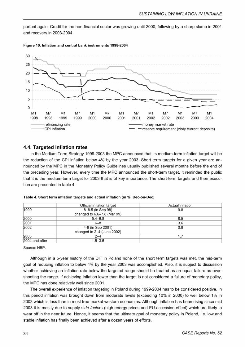
SUSTAINING LOW INFLATION IN UKRAINE
CASE Reports No. 62 34
portant again. Credit for the non-financial sector was growing until 2000, following by a sharp slump in 2001 and recovery in 2003-2004.
Figure 10. Inflation and central bank instruments 1998-2004
0
5
10
15
20
25
30
M11998
M71998
M11999
M71999
M12000
M72000
M12001
M72001
M12002
M72002
M12003
M72003
M12004
%
refinancing rate money market rateCPI inflation reserve requirement (zloty current deposits)
4.4. Targeted inflation rates In the Medium Term Strategy 1999-2003 the MPC announced that its medium-term inflation target will be
the reduction of the CPI inflation below 4% by the year 2003. Short term targets for a given year are an-nounced by the MPC in the Monetary Policy Guidelines usually published several months before the end of the preceding year. However, every time the MPC announced the short-term target, it reminded the public that it is the medium-term target for 2003 that is of key importance. The short-term targets and their execu-tion are presented in table 4.
Table 4. Short term inflation targets and actual inflation (in %, Dec-on-Dec)
Official inflation target Actual inflation 1999 8–8.5 (in Sep 98)
changed to 6.6–7.8 (Mar 99) 9.8
2000 5.4–6.8 8.5 2001 6–8 3.6 2002 4-6 (in Sep 2001)
changed to 2–4 (June 2002) 0.8
2003 2–4 1.7 2004 and after 1.5–3.5
Source: NBP.
Although in a 5-year history of the DIT in Poland none of the short term targets was met, the mid-term goal of reducing inflation to below 4% by the year 2003 was accomplished. Also, it is subject to discussion whether achieving an inflation rate below the targeted range should be treated as an equal failure as over-shooting the range. If achieving inflation lower than the target is not considered a failure of monetary policy, the MPC has done relatively well since 2001.
The overall experience of inflation targeting in Poland during 1999-2004 has to be considered positive. In this period inflation was brought down from moderate levels (exceeding 10% in 2000) to well below 1% in 2003 which is less than in most free-market western economies. Although inflation has been rising since mid 2003 it is mostly due to supply side factors (high energy prices and EU-accession effect) which are likely to wear off in the near future. Hence, it seems that the ultimate goal of monetary policy in Poland, i.e. low and stable inflation has finally been achieved after a dozen years of efforts.
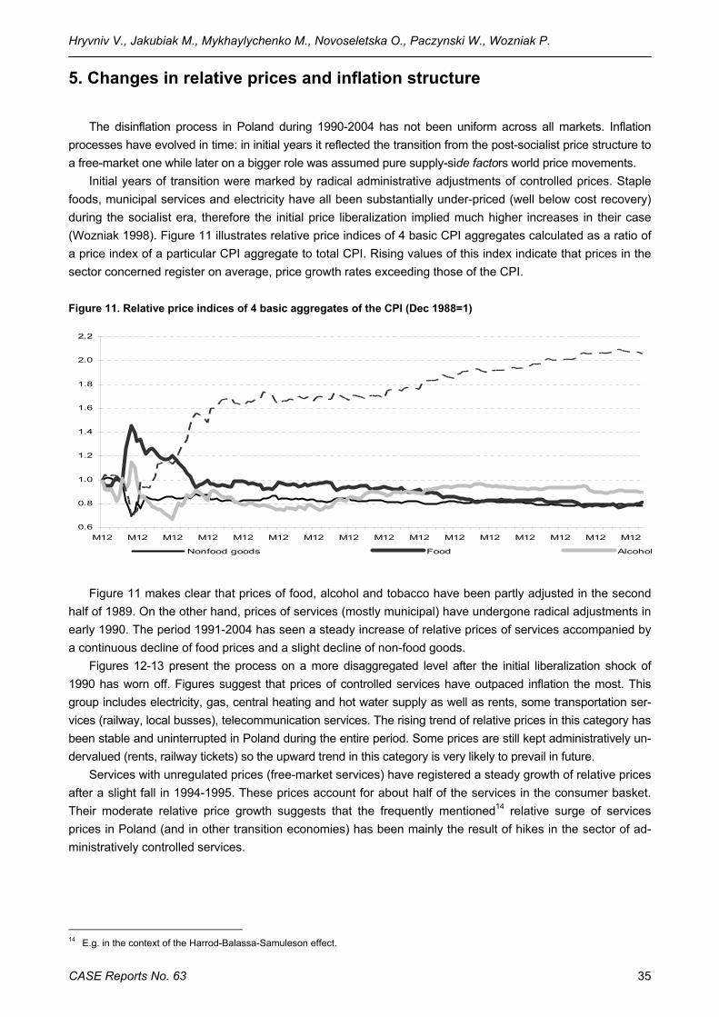
Hryvniv V., Jakubiak M., Mykhaylychenko M., Novoseletska O., Paczynski W., Wozniak P.
CASE Reports No. 63 35
5. Changes in relative prices and inflation structure
The disinflation process in Poland during 1990-2004 has not been uniform across all markets. Inflation processes have evolved in time: in initial years it reflected the transition from the post-socialist price structure to a free-market one while later on a bigger role was assumed pure supply-side factors world price movements.
Initial years of transition were marked by radical administrative adjustments of controlled prices. Staple foods, municipal services and electricity have all been substantially under-priced (well below cost recovery) during the socialist era, therefore the initial price liberalization implied much higher increases in their case (Wozniak 1998). Figure 11 illustrates relative price indices of 4 basic CPI aggregates calculated as a ratio of a price index of a particular CPI aggregate to total CPI. Rising values of this index indicate that prices in the sector concerned register on average, price growth rates exceeding those of the CPI.
Figure 11. Relative price indices of 4 basic aggregates of the CPI (Dec 1988=1)
0.6
0.8
1.0
1.2
1.4
1.6
1.8
2.0
2.2
M121988
M121989
M121990
M121991
M121992
M121993
M121994
M121995
M121996
M121997
M121998
M121999
M122000
M122001
M122002
M122003
Nonfood goods Food Alcohol
Figure 11 makes clear that prices of food, alcohol and tobacco have been partly adjusted in the second half of 1989. On the other hand, prices of services (mostly municipal) have undergone radical adjustments in early 1990. The period 1991-2004 has seen a steady increase of relative prices of services accompanied by a continuous decline of food prices and a slight decline of non-food goods.
Figures 12-13 present the process on a more disaggregated level after the initial liberalization shock of 1990 has worn off. Figures suggest that prices of controlled services have outpaced inflation the most. This group includes electricity, gas, central heating and hot water supply as well as rents, some transportation ser-vices (railway, local busses), telecommunication services. The rising trend of relative prices in this category has been stable and uninterrupted in Poland during the entire period. Some prices are still kept administratively un-dervalued (rents, railway tickets) so the upward trend in this category is very likely to prevail in future.
Services with unregulated prices (free-market services) have registered a steady growth of relative prices after a slight fall in 1994-1995. These prices account for about half of the services in the consumer basket. Their moderate relative price growth suggests that the frequently mentioned14 relative surge of services prices in Poland (and in other transition economies) has been mainly the result of hikes in the sector of ad-ministratively controlled services.
14 E.g. in the context of the Harrod-Balassa-Samuleson effect.
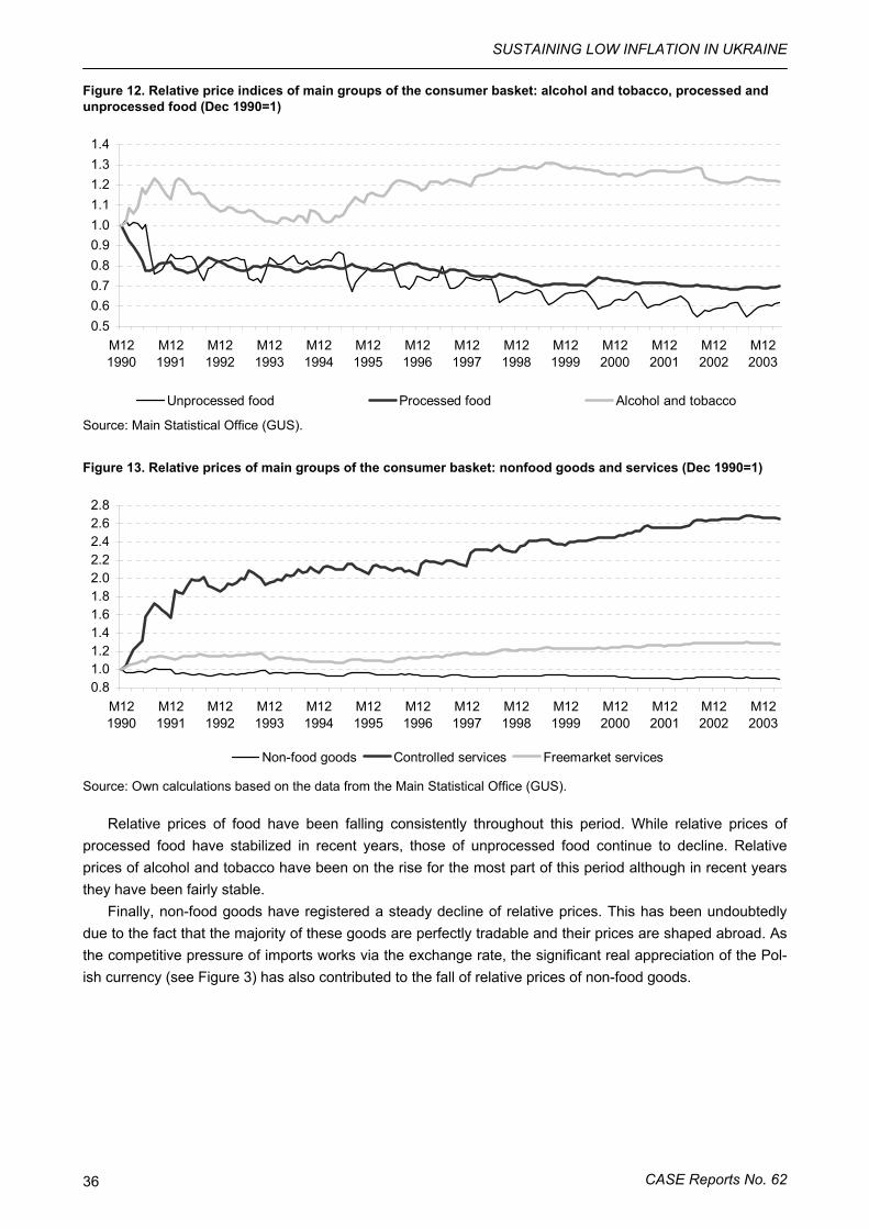
SUSTAINING LOW INFLATION IN UKRAINE
CASE Reports No. 62 36
Figure 12. Relative price indices of main groups of the consumer basket: alcohol and tobacco, processed and unprocessed food (Dec 1990=1)
0.50.60.70.80.91.01.11.21.31.4
M121990
M121991
M121992
M121993
M121994
M121995
M121996
M121997
M121998
M121999
M122000
M122001
M122002
M122003
Unprocessed food Processed food Alcohol and tobacco
Source: Main Statistical Office (GUS).
Figure 13. Relative prices of main groups of the consumer basket: nonfood goods and services (Dec 1990=1)
0.81.01.21.41.61.82.02.22.42.62.8
M121990
M121991
M121992
M121993
M121994
M121995
M121996
M121997
M121998
M121999
M122000
M122001
M122002
M122003
Non-food goods Controlled services Freemarket services
Source: Own calculations based on the data from the Main Statistical Office (GUS).
Relative prices of food have been falling consistently throughout this period. While relative prices of processed food have stabilized in recent years, those of unprocessed food continue to decline. Relative prices of alcohol and tobacco have been on the rise for the most part of this period although in recent years they have been fairly stable.
Finally, non-food goods have registered a steady decline of relative prices. This has been undoubtedly due to the fact that the majority of these goods are perfectly tradable and their prices are shaped abroad. As the competitive pressure of imports works via the exchange rate, the significant real appreciation of the Pol-ish currency (see Figure 3) has also contributed to the fall of relative prices of non-food goods.
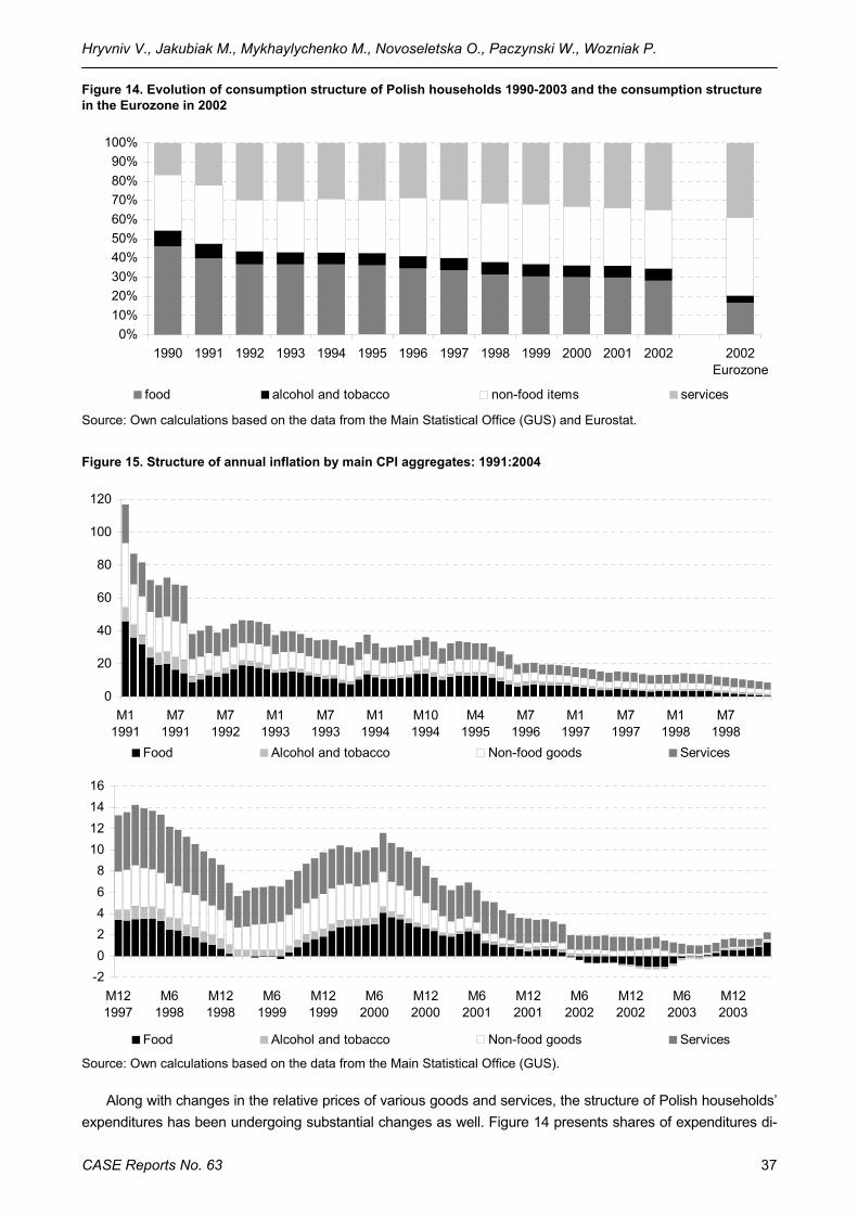
Hryvniv V., Jakubiak M., Mykhaylychenko M., Novoseletska O., Paczynski W., Wozniak P.
CASE Reports No. 63 37
Figure 14. Evolution of consumption structure of Polish households 1990-2003 and the consumption structure in the Eurozone in 2002
0%10%20%30%40%50%60%70%80%90%
100%
1990 1991 1992 1993 1994 1995 1996 1997 1998 1999 2000 2001 2002 2002Eurozone
food alcohol and tobacco non-food items services
Source: Own calculations based on the data from the Main Statistical Office (GUS) and Eurostat.
Figure 15. Structure of annual inflation by main CPI aggregates: 1991:2004
0
20
40
60
80
100
120
M11991
M71991
M71992
M11993
M71993
M11994
M101994
M41995
M71996
M11997
M71997
M11998
M71998
Food Alcohol and tobacco Non-food goods Services
-202468
10121416
M121997
M61998
M121998
M61999
M121999
M62000
M122000
M62001
M122001
M62002
M122002
M62003
M122003
Food Alcohol and tobacco Non-food goods Services
Source: Own calculations based on the data from the Main Statistical Office (GUS).
Along with changes in the relative prices of various goods and services, the structure of Polish households’ expenditures has been undergoing substantial changes as well. Figure 14 presents shares of expenditures di-
SUSTAINING LOW INFLATION IN UKRAINE
CASE Reports No. 62 38
vided into 4 basic aggregates: food, alcohol and tobacco, non-food goods and services for Poland during 1990-2003 as well as for the Eurozone for 2002 for comparative purposes. The figure makes clear that during this period the consumption structure of Polish households was converging to the one prevailing in the Eurozone. The trends present in the consumption data include a continuous increase in expenditures on services coupled with a steady decline of expenditures on food (especially unprocessed food). The share of services in house-holds’ expenditures has gone up from 17% in 1990 to 37% in 2003, while the share of food has declined from 46% in 1990 to 27% in 2003. The shares of expenditures on alcohol and tobacco as well as non-food goods have remained fairly stable at 6-6.5% and 30%, respectively, for most years in the 14-year sample.
Comparing to the most recent Polish data, the structure of expenditures in the Eurozone is characterized by higher shares of expenditures on non-food goods and services and lower for the remaining 2 categories. However, the differences are much smaller now than they used to be in early 1990s and with the prevailing trend we should expect the Polish structure to converge to the Eurozone structure within several years.
To summarize the investigation of inflation structure, it is worthwhile to see the contribution of each of the 4 basic CPI aggregates to inflation. Figure 15 presents the extent to which food, alcohol and tobacco, non-food goods and services contributed to annual inflation rates during 1991-2004. It is worthwhile to notice that the contribution of the food aggregate has been very volatile in recent years with longer periods of deflation in 1999, 2002 and 2003. Non-food goods, in line with their slightly falling relative prices (figure 11 and 13), have seen their contribution fall in recent years, while services continue, to have the highest contribution to total inflation, on average.
References
Balcerowicz, Leszek (1997) Socjalizm, kapitalizm, transformacja (Socializm, capitalizm, transformation), PWN. Bauc, Jaroslaw, Marek Dabrowski and Pawel Senator (1995) Charakterystyka zrodel inflacji w Polsce w
latach 1990-1993 (Characteristics of inflation origins in Poland 1990-1993) IN: Marek Dabrowski Polityka gospodarcza okresu transformacji (Economic policy in transition), Centrum Analiz Spoleczno-Ekonomicznych and Wydawnictwo Naukowe PWN, Warszawa.
Dabrowski, Marek (1992) The Polish Stabilization 1990-1991, Journal of International and Comparative Economics, vol.1, no.4, pp 295-324.
Kokoszczynski, Ryszard (2004) Wspolczesna polityka pieniezna a Polsce (Contemporary Monetary Policy in Poland), Panstwowe Wydawnictwo Ekonomiczne, Warszawa.
Narodowy Bank Polski (1997-2003) Raport o Inflacji (Inflation Reports). Narodowy Bank Polski (1997-2003) Zalozenia Polityki Pienieznej (Monetary Policy Guidelines). Narodowy Bank Polski (1998), Średniookresowa strategia polityki pieniężnej na lata 1999-2003 (Mid-
term Strategy of Monetary Policy). Narodowy Bank Polski (2003) Strategia Polityki Pienieznej po 2003 r. (Monetary Policy Strategy beyond
2003). Szpunar, Piotr (2002) Polityka pieniezna. Cele i warunki skutecznosci (Monetary Policy. Targets and
conditions of efficiency), Panstwowe Wydawnictwo Ekonomiczne, Warszawa. Topinski, Andrzej (1995) Polityka pieniężna w latach 1990-1992 (Monetary Policy during 1990-1992) IN:
Marek Dabrowski Polityka gospodarcza okresu transformacji (Economic policy in transition), Centrum Analiz Spoleczno-Ekonomicznych and Wydawnictwo Naukowe PWN, Warszawa.
Wellisz, Stanislaw (1997) Inflation and Stabilization in Poland 1990-95, IN: Mario I. Blejer and Marko Skreb Macroeconomic Stabilization in Transition Economies, Cambridge University Press, Cambridge.
Woźniak, Przemysław (1998) Relative Prices and Inflation in Poland 1989-1997, Policy Research Work-ing Paper 1879, The World Bank.
Hryvniv V., Jakubiak M., Mykhaylychenko M., Novoseletska O., Paczynski W., Wozniak P.
CASE Reports No. 63 39
Chapter 4: Analysis of Core Inflation Indicators in Ukraine
Przemyslaw Wozniak, Mykyta Mykhaylychenko
1. Introduction
Since the end of the 1970s fighting inflation became an issue of highest priority in most countries. Target-ing inflation, whether direct (in the form of the Direct Inflation Targeting strategy) or indirect, in the majority of cases implies aiming to achieve a specific rate of annual growth of the Consumer Price Index (CPI), i.e. the index that measures the percentage change in the cost of a variety of goods and services comprising the consumers’ basket. As such, it is publicized and well known and the target itself is therefore transparent and well understood. However, it is also widely acknowledged that the CPI is a rather deficient indicator of the “trend” inflation especially if measured at high frequencies such as quarters or months. Monthly or quarterly series are usually highly volatile, seasonal and contain a lot of noise. Given the insufficient knowledge of the nature of transmission processes, monetary authorities need some firm guidelines that would help shape their policy to produce the targeted rate of inflation. Most importantly, they need to distinguish between movements in inflation that are transitory and those that are symptoms of the persistent drift of prices. Roger (1995) notes that as long as perceived CPI changes reflect one-time shocks to the general price level (such as for example, a change in the tax rate), or one-off shifts in relative prices, they should not provoke any ac-tion on the part of monetary authorities15.
Therefore, the ideal measure of core inflation should account for the long-term trend movements in prices that reflect the state of demand in the economy and discard various one-off shocks coming from the supply side. This idea of excluding all shocks with no demand-side provenience stems essentially from the main-stream economics view that “monetary policy works primarily through its influence over demand pressures in the economy” (Roger 1995). Therefore one can only hold monetary authorities accountable for inflation that arises from those pressures, i.e. inflation whose elements lie within their direct influence. To see why this is a reasonable setup, one might think of a frequently exploited example of bad harvest caused by unfavorable weather. High prices of agricultural products due to a smaller-than-usual supply would certainly drive raise foodstuffs’ prices up and the entire CPI would pick up temporarily. If monetary authorities followed the CPI movements closely this would prompt a “tightening” action on their part as the targeted variable moved out of the band. But this can hardly be considered a right policy to pursue as the registered rise in inflation is not a symptom of the new permanent trend or but rather reflects a temporary shift in relative prices.
This simple example provides intuition for what is not at all a trivial problem. How to filter out transitory noise out of price data and construct a measure that can serve as an appropriate guideline for monetary au-thorities? This paper aims to shed some light on the answer to this complex question in the context of Ukrainian inflation data. Inflation developments in Ukraine have been highly unpredictable in recent years: 15 Unless monetary authorities target price level.
SUSTAINING LOW INFLATION IN UKRAINE
CASE Reports No. 62 40
annual deflation prevailed in the second half of 2002, after which inflation was on a steady rise in 2003 and is now back to moderate levels at 7-8% on an annual basis. High volatility of the CPI inflation makes it more difficult for Ukrainian policymakers to filter out transitory short-term fluctuations and correctly predict the infla-tion trend. Core inflation constitutes a potential solution to this problem. It provides the authorities with a more stable and reliable measure of inflation and is thus a highly desirable policy tool in Ukraine.
In view of the absence of one widely accepted theoretical definition of core inflation, methods of calculat-ing core inflation have proliferated in last 2 decades. Each of them renders itself further to parameterization and owing to numerous values for these parameters, the resulting population of core inflation estimates is virtually infinite. To the extent that all series differ in the way they filter the data, it is necessary to find a sta-tistical method that reflects core price movements in a relatively most efficient and robust way. In this paper we suggest a complete and methodologically coherent technique of comparing and choosing between vari-ous core inflation indicators and then apply it to the Ukrainian inflation data.
The paper is composed as follows. Part 2 reviews the most important conceptual issues related to core inflation as well as introduces 5 statistical methods of estimating core inflation indicators. Part 3 presents and analyzes descriptive statistics of empirical distributions of disaggregated CPI in Ukraine and provides further rationale for using statistical techniques of estimating core inflation. Part 4 introduces the 3 criteria used in evaluating core inflation indicators and applies them to the population of empirical series of Ukrainian core inflation indicators. These criteria provide a tool for singling out optimal core inflation series for each method separately as well as for indicating the series that can be considered the optimal indicator within the entire population of core inflation series. Finally, part 5 concludes with summary and recommendations.
2. Core inflation – theory and practice
2.1. General considerations Literature suggests two general broad categories of problems that arise when one deals with typically
collected price data. Using the terminology borrowed from econometrics they will be labeled noise and bias. Noise refers to all transitory shocks that are assumed to add up to zero in the long run, but exert tempo-
rary and noticeable influence on prices in the short run (especially when data is reported at high frequencies such as month or quarter). This category encompasses all kinds of shocks that originate in the supply side of the economy, such as seasonal phenomena, broadly defined resource shocks as well as shocks related to exchange or tax rate changes or any other shocks inducing shifts in relative prices. As indicated earlier all these shocks cancel out when one looks at a longer horizon but introduce undesirable fluctuations at high frequencies. Eliminating noise will be the primary focus of this study.
Bias in the context of price data is usually thought of as being either weighting bias or measurement bias. The former is rather unlikely to play a substantial role in the Ukrainian data since it is essentially related to infrequent adjustment of consumption weights. The Ukrainian Statistical Office belongs to a group of statisti-cal agencies that carry out expenditure surveys every year and adjust the weights accordingly. Therefore, the bias that arises as constant weights do not account for relative price shifts, may be harmlessly neglected. Measurement bias refers to actual errors in measuring individual prices16. It is the subject of numerous stud-ies done mostly in the context of US price data17 and since it is essentially different in nature than noise it will not be elaborated upon in this paper.
Cecchetti (1996) gives a simple formalized accounting framework wrapping up the preceding discussion in formulas. Following his notation, we define:
16 Cecchetti [1996] gives quality and new goods bias as examples of measurement bias. 17 See Wynne and Sigalla[1993] and Shapiro and Wilcox[1996] for detailed discussion and actual bias estimates for the US.

Hryvniv V., Jakubiak M., Mykhaylychenko M., Novoseletska O., Paczynski W., Wozniak P.
CASE Reports No. 63 41
(1) ittit xPp += is the rate of change in the price of an individual CPI item – i According to the formula it is composed of
tP – the trend movement and the best approximation of the underlying inflation and
itx – relative price inflation that represents one-time movements inherent in an individual item and not representative of the core trend.
Now, the regular “headline” CPI is just the weighted average of all the items: (2) ∑≡ i ititt pwπ where wit‘s represent expenditure basket weights and add up to unity for each t.
or, combining (1) and (2) (3) ∑+=
i itittt xwPπ .
The second term in (3) is of most interest from the point of view of measuring core inflation. It represents the cluster of noise (nt) and bias (bt) that is attached to the “real” inflation period by period for all t’s. Writing more explicitly: (4) tti itittt bnxwP +==− ∑π
where noise or nt has zero mean and is stationary and bias bt can be further decomposed into a constant (μb) and a zero-mean transitory component (ωt): (5) tbtb ωμ +=
If we define inflation of an individual item i over k periods as
(6) it
itkitkit p
ppp
−= +
this yields the following definition of the aggregate price inflation:
(7) ( )∑ = ++ +++=k
j jtjtbk
tkt nP
1ωμπ
In line with the earlier discussion, the assumption is being made that the weighting bias – ωt is rather in-significant in the Ukrainian price data. As for the measurement bias represented by the constant term – μt , it might very well be present in the data, however, it will not be discussed in this paper18. It follows from the definition of the noise (in particular from zero mean assumption) that when the number of elements (k) in the right-hand side sum in (7) is sufficiently large, nt’s cancel each other out and the whole summation collapses to zero. In the context of inflation rates this means that with the change of frequency from monthly to 12-monthly, πt should get closer to k
tP which represents the core inflation. From (7) it is also clear that taking averages of inflation over longer periods will do the job too as high-
frequency noise averaged over longer time horizon is likely to move closer to zero. However, averaging infla-tion rates in order to approximate trend price movements is not a good option for policy makers who need timely measures, that is, indicators available for use in the first instance.19
Ideal estimators of core inflation should also be robust, i.e. relatively insensitive to particular cases (or, in the context of this study, individual price distributions). Robust estimators may not be optimal for every single situation, but their useful feature is good and reliable performance even in extreme settings.
Another desirable characteristic of a good estimator is unbiasedness. It is clear that any good measure of core inflation must hit the “real” core inflation on average. Otherwise, it will tend to mislead us and either over- or understate the core price movements.
18 The measurement bias should not weaken the conceptual framework of the analysis presented in this paper since as a constant it
does not interact with the time-variable noise. 19 It is obvious that averages will fail as timely measures as one needs some “future” (t>0) observations in order to calculate a contem-
poraneous (i.e. t=0) measure.
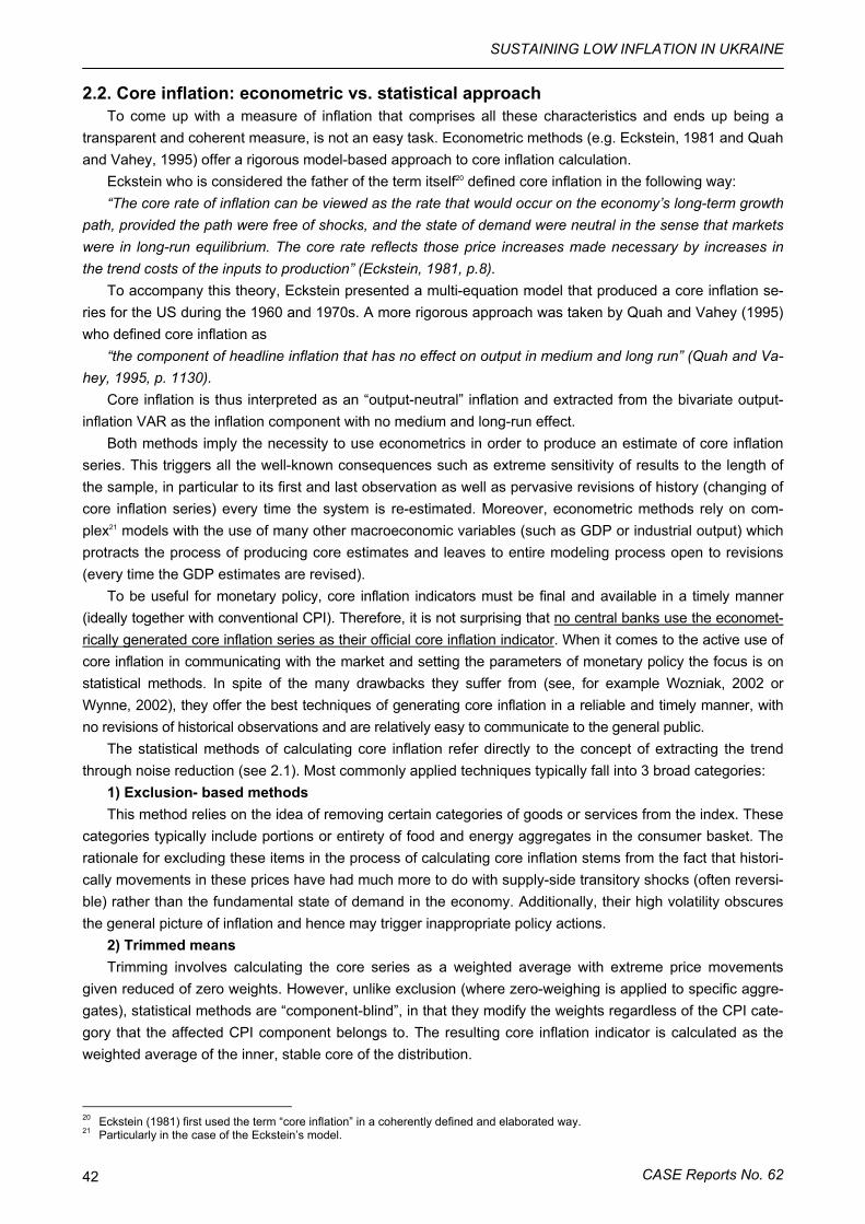
SUSTAINING LOW INFLATION IN UKRAINE
CASE Reports No. 62 42
2.2. Core inflation: econometric vs. statistical approach To come up with a measure of inflation that comprises all these characteristics and ends up being a
transparent and coherent measure, is not an easy task. Econometric methods (e.g. Eckstein, 1981 and Quah and Vahey, 1995) offer a rigorous model-based approach to core inflation calculation.
Eckstein who is considered the father of the term itself20 defined core inflation in the following way: “The core rate of inflation can be viewed as the rate that would occur on the economy’s long-term growth
path, provided the path were free of shocks, and the state of demand were neutral in the sense that markets were in long-run equilibrium. The core rate reflects those price increases made necessary by increases in the trend costs of the inputs to production” (Eckstein, 1981, p.8).
To accompany this theory, Eckstein presented a multi-equation model that produced a core inflation se-ries for the US during the 1960 and 1970s. A more rigorous approach was taken by Quah and Vahey (1995) who defined core inflation as
“the component of headline inflation that has no effect on output in medium and long run” (Quah and Va-hey, 1995, p. 1130).
Core inflation is thus interpreted as an “output-neutral” inflation and extracted from the bivariate output-inflation VAR as the inflation component with no medium and long-run effect.
Both methods imply the necessity to use econometrics in order to produce an estimate of core inflation series. This triggers all the well-known consequences such as extreme sensitivity of results to the length of the sample, in particular to its first and last observation as well as pervasive revisions of history (changing of core inflation series) every time the system is re-estimated. Moreover, econometric methods rely on com-plex21 models with the use of many other macroeconomic variables (such as GDP or industrial output) which protracts the process of producing core estimates and leaves to entire modeling process open to revisions (every time the GDP estimates are revised).
To be useful for monetary policy, core inflation indicators must be final and available in a timely manner (ideally together with conventional CPI). Therefore, it is not surprising that no central banks use the economet-rically generated core inflation series as their official core inflation indicator. When it comes to the active use of core inflation in communicating with the market and setting the parameters of monetary policy the focus is on statistical methods. In spite of the many drawbacks they suffer from (see, for example Wozniak, 2002 or Wynne, 2002), they offer the best techniques of generating core inflation in a reliable and timely manner, with no revisions of historical observations and are relatively easy to communicate to the general public.
The statistical methods of calculating core inflation refer directly to the concept of extracting the trend through noise reduction (see 2.1). Most commonly applied techniques typically fall into 3 broad categories:
1) Exclusion- based methods This method relies on the idea of removing certain categories of goods or services from the index. These
categories typically include portions or entirety of food and energy aggregates in the consumer basket. The rationale for excluding these items in the process of calculating core inflation stems from the fact that histori-cally movements in these prices have had much more to do with supply-side transitory shocks (often reversi-ble) rather than the fundamental state of demand in the economy. Additionally, their high volatility obscures the general picture of inflation and hence may trigger inappropriate policy actions.
2) Trimmed means Trimming involves calculating the core series as a weighted average with extreme price movements
given reduced of zero weights. However, unlike exclusion (where zero-weighing is applied to specific aggre-gates), statistical methods are “component-blind”, in that they modify the weights regardless of the CPI cate-gory that the affected CPI component belongs to. The resulting core inflation indicator is calculated as the weighted average of the inner, stable core of the distribution.
20 Eckstein (1981) first used the term “core inflation” in a coherently defined and elaborated way. 21 Particularly in the case of the Eckstein’s model.

Hryvniv V., Jakubiak M., Mykhaylychenko M., Novoseletska O., Paczynski W., Wozniak P.
CASE Reports No. 63 43
Ordinary trimmed means The most common category within this group are ordinary trimmed means. Calculating simple trimmed
means involves discarding (or zero-weighing) a certain percentage of CPI components (based on their share in the basket) from both ends of the distribution of individual inflation rates and computing the weighted av-erage of the rest. Symmetric trims zero-weigh the same percentage at both ends so that k% trimmed mean eliminates k/2 %22 highest and k/2% lowest price movements during the period concerned and takes the weighted mean of the middle (100-k)%. Asymmetric means distribute the trim asymmetrically. A special case of a trimmed mean is the usual CPI ( 0% trimmed mean) and percentiles that are 100% trimmed means (specifically, median is a symmetric 100% trimmed mean). Thus, ordinary trimmed means are characterized by 2 parameters: total trim (t) and the asymmetry of trimming (a).
Means trimmed according to the distance from the center of the distribution In the case of this type of trimmed means, the criterion for trimming is the distance from the center of the
distribution of cross-sectional price changes. In simple terms, this method eliminates all the components whose prices changed much more or much less than the average.
The new weight system changes every month and can be written as follows:
(7) ⎪⎩
⎪⎨
⎧
+>∀
+≤∀=
tVtiti
tVtitiiw
iwτμπ
τμπ
for 0
for ~ , where
μt is the center of the price change distribution during a particular month t defined for example as the weighted mean, τ is a non-negative number, Vt is the volatility measure of individual inflation indices during time t, for example, variance of the cross-section distribution.
In the re-weighting process items with unrepresentative price changes are zero-weighted and items with price changes close to the average are left with the original weight.
Means trimmed according to price stability The trimming criterion used here refers to volatility. This method aims at reducing noise by eliminating
those components whose variance ratio (to the variance of the CPI) is higher than some cut-off threshold. The implied new weight structure is as follows:
(8)
⎪⎪⎩
⎪⎪⎨
⎧
>∀
<∀=
γσσ
γσσ
π
2
2
2
2
***
for 0
for
i
i
i
i
ii
i
ww , where
γ is a non-negative number, σ2 stands for the variance of individual items of the basket (in numerator) or the aggregate CPI (in denominator).
3) Variance-weighted means The main principle of calculating variance-weighted means is to reduce noise by substituting completely
or augmenting consumption-related weights with weights proportional to volatility. The system of re-weighting implies that no items are zero-weighted (which was the case in all 4 preceding methods), but instead, basket elements are given weights inversely proportional to their volatility. Four different types of variance weighted means will be calculated in this paper with the following modified weight systems23:
22 Where percentages refer to basket weights rather than the number of categories. 23 All weight structures presented below are scaled to unity.

SUSTAINING LOW INFLATION IN UKRAINE
CASE Reports No. 62 44
Type I: Complete substitution with reciprocal of individual variances
(9) ∑ =
= N
i i
iiw
12
21
/1
/1
σ
σ.
Type II: Partial substitution in which consumption weights remain but are augmented (multiplied) by re-ciprocal of individual variances
(10)
∑ =
=N
ii
i
i
i
i w
w
w
1 2
22
σ
σ.
Type III: Partial substitution with reciprocal of variances of relative price changes: πi – πCPI
(11)
∑ =−
−=N
ii
i
ii
i
i
i
w
ww
1),(
),(3
1
ππ
ππ
σ
σ.
Applying such alternative weighting systems ensures that each CPI component gets a weight propor-tional to the quality and strength of the inflation signal it carries. The contribution of volatile items to the index is reduced while that of stable items is magnified. The end result is a core inflation indicator that indicates the trend inflation movement to a much bigger extent than does the CPI which contains a lot of noise coming from volatile items.
Methods based on crude exclusion (method 1) are very good in that they are concise, simple, and offer a very appealing alternative to the conventional CPI. Their widespread use as indicators of trend inflation does, however, raise of couple of important objections. To the extent that the ideal measure of core inflation should make use of all available price information about long-run inflation trends, is permanent exclusion of food and energy prices always justified? In other words, is it always the case that those price movements convey no such information? Certainly not, and it seems logical to try to construct a measure of underlying inflation that would make use of valuable price information in a more flexible way without automatically discarding specific CPI categories like the first two methods described above. Trimmed means and variance weighted means (methods 2 and 3) seem to fulfill the conditions of an efficient use of available price information and are based to a smaller extent on ad-hoc judgment and discretion.
Throughout the paper several terms will be used interchangeably. Core inflation will be sometimes called underlying or trend inflation. CPI inflation will be referred to as “headline” rate inflation or simply, conventional rate of inflation.
3. Empirical distributions of disaggregated CPI
3.1. Description of the data To date, core inflation for Ukraine has been estimated by Petrik and Polovnyov (2002, 2003). However,
their analysis concerns only monthly inflation rates which, due to seasonality, are a much less important meas-ure of inflationary pressures than annual rates. In their 2002 paper Petrik and Polovnyov calculated one exclu-sion-based indicator for the period 1999:1-2002:5 while their 2003 study includes 3 basic indicators (exclusion, trimmed mean and a median) as well as a moving average and covers the period of 1999:1-2003:4.
Our study is fundamentally different in that we make use of annual inflation rates and apply various theo-retical criteria to make a choice of an optimal core inflation indicator for Ukraine. Our analysis also covers the
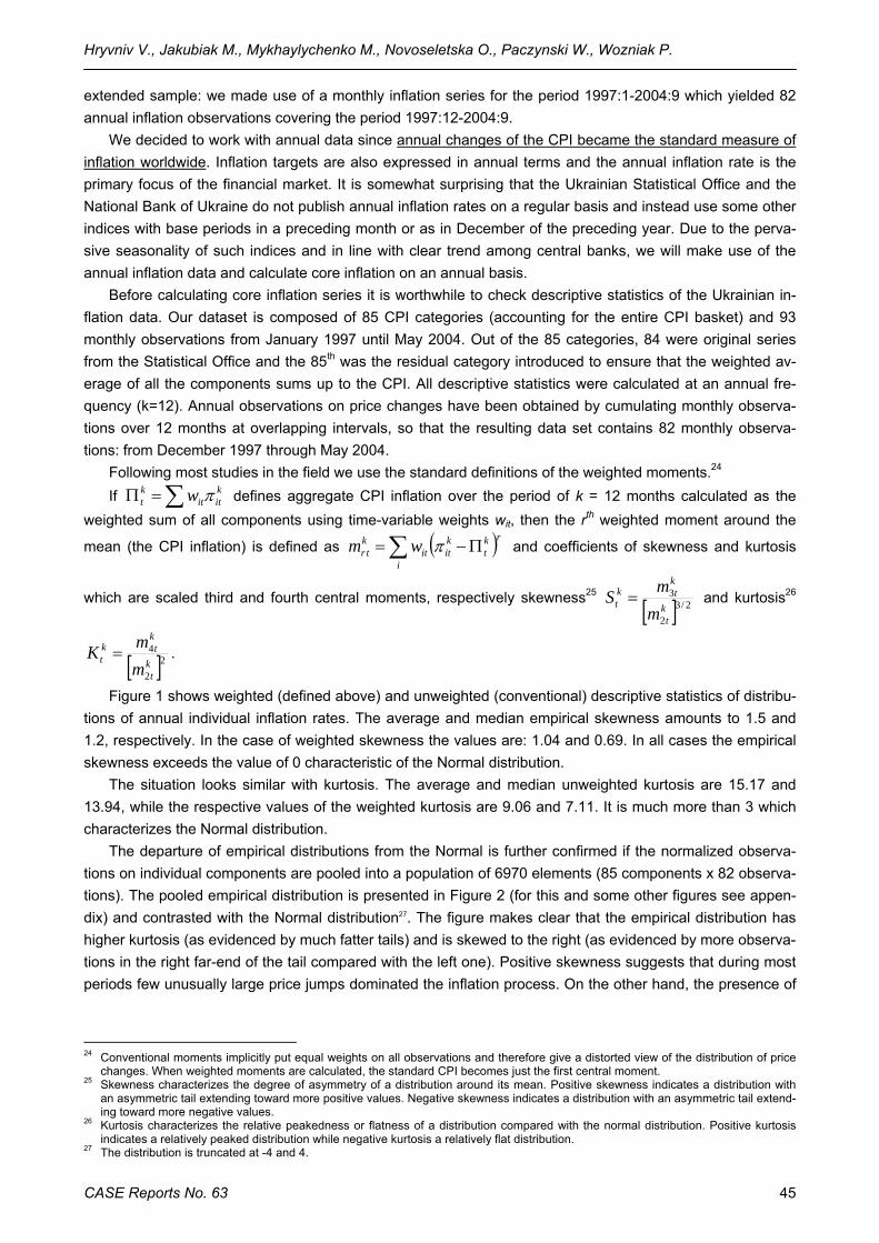
Hryvniv V., Jakubiak M., Mykhaylychenko M., Novoseletska O., Paczynski W., Wozniak P.
CASE Reports No. 63 45
extended sample: we made use of a monthly inflation series for the period 1997:1-2004:9 which yielded 82 annual inflation observations covering the period 1997:12-2004:9.
We decided to work with annual data since annual changes of the CPI became the standard measure of inflation worldwide. Inflation targets are also expressed in annual terms and the annual inflation rate is the primary focus of the financial market. It is somewhat surprising that the Ukrainian Statistical Office and the National Bank of Ukraine do not publish annual inflation rates on a regular basis and instead use some other indices with base periods in a preceding month or as in December of the preceding year. Due to the perva-sive seasonality of such indices and in line with clear trend among central banks, we will make use of the annual inflation data and calculate core inflation on an annual basis.
Before calculating core inflation series it is worthwhile to check descriptive statistics of the Ukrainian in-flation data. Our dataset is composed of 85 CPI categories (accounting for the entire CPI basket) and 93 monthly observations from January 1997 until May 2004. Out of the 85 categories, 84 were original series from the Statistical Office and the 85th was the residual category introduced to ensure that the weighted av-erage of all the components sums up to the CPI. All descriptive statistics were calculated at an annual fre-quency (k=12). Annual observations on price changes have been obtained by cumulating monthly observa-tions over 12 months at overlapping intervals, so that the resulting data set contains 82 monthly observa-tions: from December 1997 through May 2004.
Following most studies in the field we use the standard definitions of the weighted moments.24 If ∑=Π k
ititkt w π defines aggregate CPI inflation over the period of k = 12 months calculated as the
weighted sum of all components using time-variable weights wit, then the rth weighted moment around the
mean (the CPI inflation) is defined as ( )∑ Π−=i
rkt
kitit
ktr wm π and coefficients of skewness and kurtosis
which are scaled third and fourth central moments, respectively skewness25 [ ] 2/32
3kt
ktk
tmmS = and kurtosis26
[ ]22
4kt
ktk
tmmK = .
Figure 1 shows weighted (defined above) and unweighted (conventional) descriptive statistics of distribu-tions of annual individual inflation rates. The average and median empirical skewness amounts to 1.5 and 1.2, respectively. In the case of weighted skewness the values are: 1.04 and 0.69. In all cases the empirical skewness exceeds the value of 0 characteristic of the Normal distribution.
The situation looks similar with kurtosis. The average and median unweighted kurtosis are 15.17 and 13.94, while the respective values of the weighted kurtosis are 9.06 and 7.11. It is much more than 3 which characterizes the Normal distribution.
The departure of empirical distributions from the Normal is further confirmed if the normalized observa-tions on individual components are pooled into a population of 6970 elements (85 components x 82 observa-tions). The pooled empirical distribution is presented in Figure 2 (for this and some other figures see appen-dix) and contrasted with the Normal distribution27. The figure makes clear that the empirical distribution has higher kurtosis (as evidenced by much fatter tails) and is skewed to the right (as evidenced by more observa-tions in the right far-end of the tail compared with the left one). Positive skewness suggests that during most periods few unusually large price jumps dominated the inflation process. On the other hand, the presence of
24 Conventional moments implicitly put equal weights on all observations and therefore give a distorted view of the distribution of price
changes. When weighted moments are calculated, the standard CPI becomes just the first central moment. 25 Skewness characterizes the degree of asymmetry of a distribution around its mean. Positive skewness indicates a distribution with
an asymmetric tail extending toward more positive values. Negative skewness indicates a distribution with an asymmetric tail extend-ing toward more negative values.
26 Kurtosis characterizes the relative peakedness or flatness of a distribution compared with the normal distribution. Positive kurtosis indicates a relatively peaked distribution while negative kurtosis a relatively flat distribution.
27 The distribution is truncated at -4 and 4.
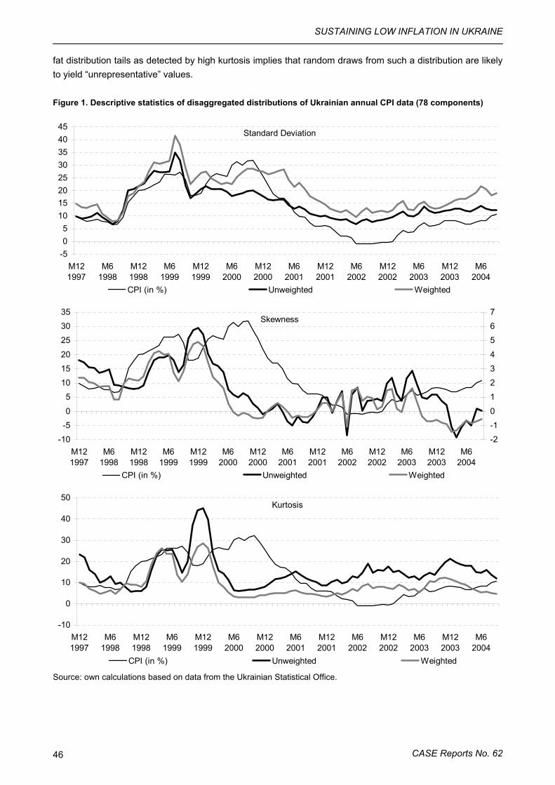
SUSTAINING LOW INFLATION IN UKRAINE
CASE Reports No. 62 46
fat distribution tails as detected by high kurtosis implies that random draws from such a distribution are likely to yield “unrepresentative” values.
Figure 1. Descriptive statistics of disaggregated distributions of Ukrainian annual CPI data (78 components)
-505
1015202530354045
M121997
M61998
M121998
M61999
M121999
M62000
M122000
M62001
M122001
M62002
M122002
M62003
M122003
M62004
CPI (in %) Unweighted Weighted
Standard Deviation
-10-50
5101520
253035
M121997
M61998
M121998
M61999
M121999
M62000
M122000
M62001
M122001
M62002
M122002
M62003
M122003
M62004
-2-10
1234
567
CPI (in %) Unweighted Weighted
Skewness
-10
0
10
20
30
40
50
M121997
M61998
M121998
M61999
M121999
M62000
M122000
M62001
M122001
M62002
M122002
M62003
M122003
M62004
CPI (in %) Unweighted Weighted
Kurtosis
Source: own calculations based on data from the Ukrainian Statistical Office.
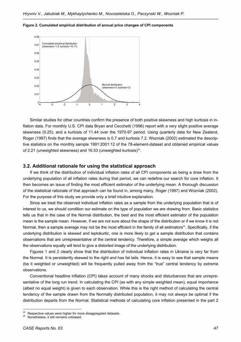
Hryvniv V., Jakubiak M., Mykhaylychenko M., Novoseletska O., Paczynski W., Wozniak P.
CASE Reports No. 63 47
Figure 2. Cumulated empirical distribution of annual price changes of CPI components
-4 -3 -2 -1 0 1 2 3 40
0.01
0.02
0.03
0.04
0.05
0.06
0.07
0.08
Normal distribution(skewness=0, kurtosis=3)
Cumulated empirical distribution(skewness=1.5, kurtosis=15.17)
Similar studies for other countries confirm the presence of both positive skewness and high kurtosis in in-flation data. For monthly U.S. CPI data Bryan and Cecchetti (1996) report with a very slight positive average skewness (0.25), and a kurtosis of 11.44 over the 1970-97 period. Using quarterly data for New Zealand, Roger (1997) finds that the average skewness is 0.7 and kurtosis 7.2. Wozniak (2002) estimated the descrip-tive statistics on the monthly sample 1991:2001:12 of the 78-element-dataset and obtained empirical values of 2.21 (unweighted skewness) and 16.53 (unweighted kurtosis)28.
3.2. Additional rationale for using the statistical approach If we think of the distribution of individual inflation rates of all CPI components as being a draw from the
underlying population of all inflation rates during that period, we can redefine our search for core inflation. It then becomes an issue of finding the most efficient estimator of the underlying mean. A thorough discussion of the statistical rationale of that approach can be found in, among many, Roger (1997) and Wozniak (2002). For the purpose of this study we provide only a brief intuitive explanation.
Since we treat the observed individual inflation rates as a sample from the underlying population that is of interest to us, we should condition our estimate on the type of population we are drawing from. Basic statistics tells us that in the case of the Normal distribution, the best and the most efficient estimator of the population mean is the sample mean. However, if we are not sure about the shape of the distribution or if we know it is not Normal, then a sample average may not be the most efficient in the family of all estimators29. Specifically, if the underlying distribution is skewed and leptokurtic, one is more likely to get a sample distribution that contains observations that are unrepresentative of the central tendency. Therefore, a simple average which weighs all the observations equally will tend to give a distorted image of the underlying distribution.
Figures 1 and 2 clearly show that the distribution of individual inflation rates in Ukraine is very far from the Normal. It is persistently skewed to the right and has fat tails. Hence, it is easy to see that sample means (be it weighted or unweighted) will be frequently pulled away from the “true” central tendency by extreme observations.
Conventional headline inflation (CPI) takes account of many shocks and disturbances that are unrepre-sentative of the long run trend. In calculating the CPI (as with any simple weighted mean), equal importance (albeit no equal weight) is given to each observation. While this is the right method of calculating the central tendency of the sample drawn from the Normally distributed population, it may not always be optimal if the distribution departs from the Normal. Statistical methods of calculating core inflation presented in the part 2
28 Respective values were higher for more disaggregated datasets. 29 Nonetheless, it still remains unbiased.
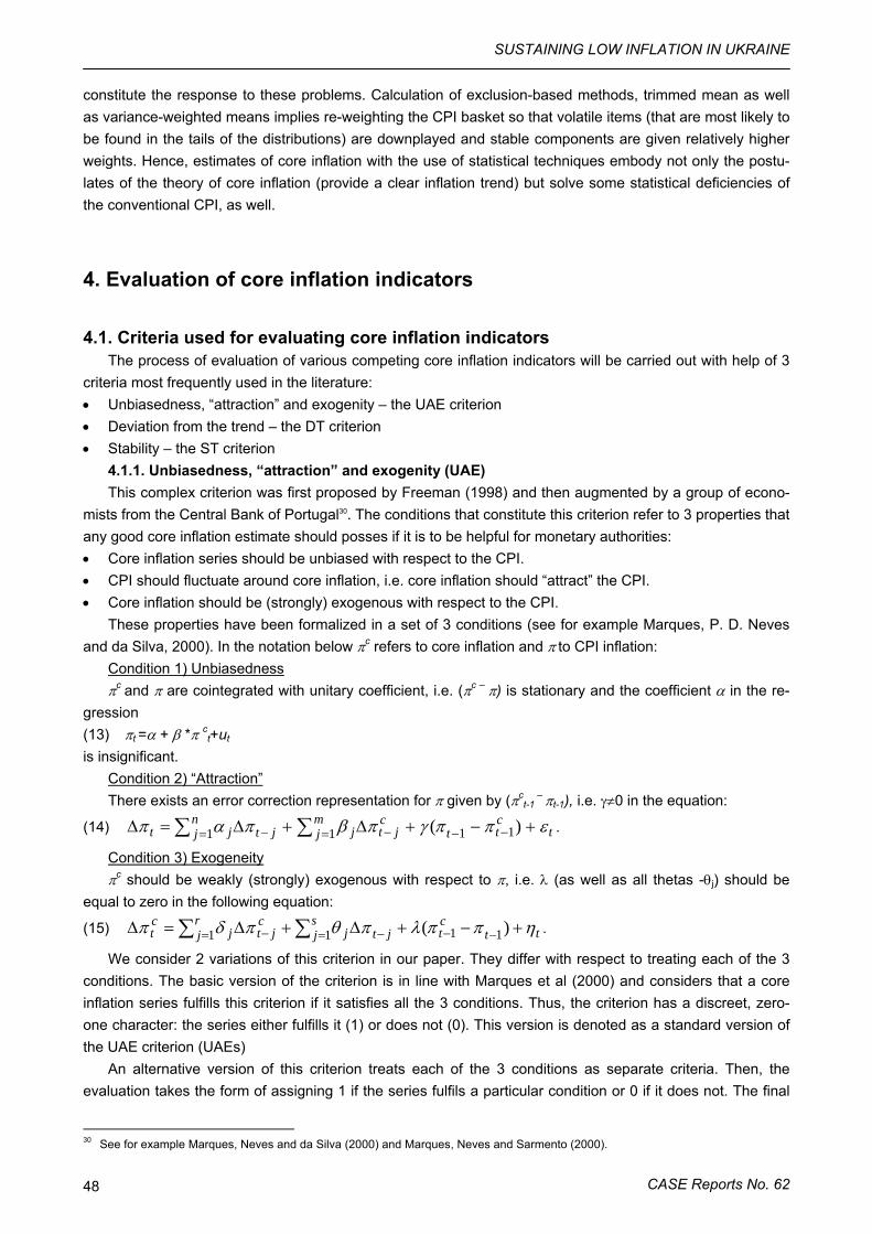
SUSTAINING LOW INFLATION IN UKRAINE
CASE Reports No. 62 48
constitute the response to these problems. Calculation of exclusion-based methods, trimmed mean as well as variance-weighted means implies re-weighting the CPI basket so that volatile items (that are most likely to be found in the tails of the distributions) are downplayed and stable components are given relatively higher weights. Hence, estimates of core inflation with the use of statistical techniques embody not only the postu-lates of the theory of core inflation (provide a clear inflation trend) but solve some statistical deficiencies of the conventional CPI, as well.
4. Evaluation of core inflation indicators
4.1. Criteria used for evaluating core inflation indicators The process of evaluation of various competing core inflation indicators will be carried out with help of 3
criteria most frequently used in the literature: • Unbiasedness, “attraction” and exogenity – the UAE criterion • Deviation from the trend – the DT criterion • Stability – the ST criterion
4.1.1. Unbiasedness, “attraction” and exogenity (UAE) This complex criterion was first proposed by Freeman (1998) and then augmented by a group of econo-
mists from the Central Bank of Portugal30. The conditions that constitute this criterion refer to 3 properties that any good core inflation estimate should posses if it is to be helpful for monetary authorities: • Core inflation series should be unbiased with respect to the CPI. • CPI should fluctuate around core inflation, i.e. core inflation should “attract” the CPI. • Core inflation should be (strongly) exogenous with respect to the CPI.
These properties have been formalized in a set of 3 conditions (see for example Marques, P. D. Neves and da Silva, 2000). In the notation below πc refers to core inflation and π to CPI inflation:
Condition 1) Unbiasedness πc and π are cointegrated with unitary coefficient, i.e. (πc – π) is stationary and the coefficient α in the re-
gression (13) πt =α + β *π ct+ut is insignificant.
Condition 2) “Attraction” There exists an error correction representation for π given by (πc
t-1 – πt-1), i.e. γ≠0 in the equation:
(14) tctt
mj
cjtj
nj jtjt εππγπβπαπ +−+Δ+Δ=Δ −−= −= − ∑∑ )( 1111 .
Condition 3) Exogeneity πc should be weakly (strongly) exogenous with respect to π, i.e. λ (as well as all thetas -θj) should be
equal to zero in the following equation:
(15) ttct
sj jtj
rj
cjtj
ct ηππλπθπδπ +−+Δ+Δ=Δ −−= −= − ∑∑ )( 1111 .
We consider 2 variations of this criterion in our paper. They differ with respect to treating each of the 3 conditions. The basic version of the criterion is in line with Marques et al (2000) and considers that a core inflation series fulfills this criterion if it satisfies all the 3 conditions. Thus, the criterion has a discreet, zero-one character: the series either fulfills it (1) or does not (0). This version is denoted as a standard version of the UAE criterion (UAEs)
An alternative version of this criterion treats each of the 3 conditions as separate criteria. Then, the evaluation takes the form of assigning 1 if the series fulfils a particular condition or 0 if it does not. The final
30 See for example Marques, Neves and da Silva (2000) and Marques, Neves and Sarmento (2000).
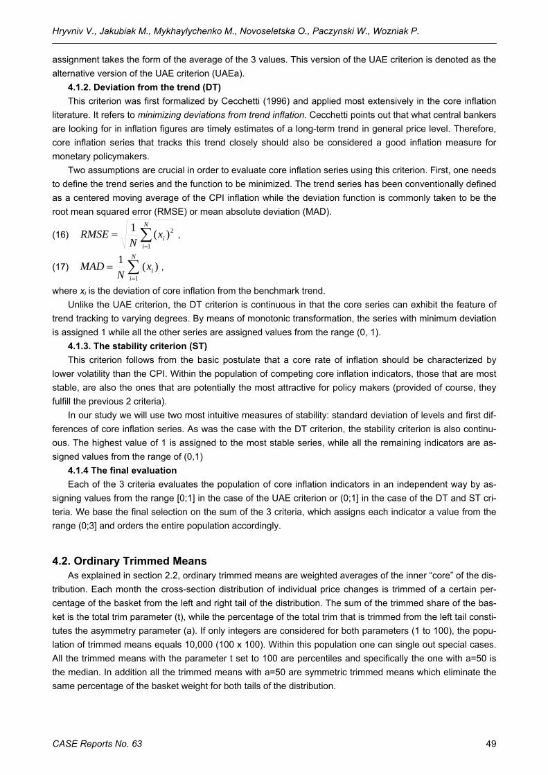
Hryvniv V., Jakubiak M., Mykhaylychenko M., Novoseletska O., Paczynski W., Wozniak P.
CASE Reports No. 63 49
assignment takes the form of the average of the 3 values. This version of the UAE criterion is denoted as the alternative version of the UAE criterion (UAEa).
4.1.2. Deviation from the trend (DT) This criterion was first formalized by Cecchetti (1996) and applied most extensively in the core inflation
literature. It refers to minimizing deviations from trend inflation. Cecchetti points out that what central bankers are looking for in inflation figures are timely estimates of a long-term trend in general price level. Therefore, core inflation series that tracks this trend closely should also be considered a good inflation measure for monetary policymakers.
Two assumptions are crucial in order to evaluate core inflation series using this criterion. First, one needs to define the trend series and the function to be minimized. The trend series has been conventionally defined as a centered moving average of the CPI inflation while the deviation function is commonly taken to be the root mean squared error (RMSE) or mean absolute deviation (MAD).
(16) ∑=
=N
iix
NRMSE
1
2)(1,
(17) ∑=
=N
iix
NMAD
1
)(1,
where xi is the deviation of core inflation from the benchmark trend. Unlike the UAE criterion, the DT criterion is continuous in that the core series can exhibit the feature of
trend tracking to varying degrees. By means of monotonic transformation, the series with minimum deviation is assigned 1 while all the other series are assigned values from the range (0, 1).
4.1.3. The stability criterion (ST) This criterion follows from the basic postulate that a core rate of inflation should be characterized by
lower volatility than the CPI. Within the population of competing core inflation indicators, those that are most stable, are also the ones that are potentially the most attractive for policy makers (provided of course, they fulfill the previous 2 criteria).
In our study we will use two most intuitive measures of stability: standard deviation of levels and first dif-ferences of core inflation series. As was the case with the DT criterion, the stability criterion is also continu-ous. The highest value of 1 is assigned to the most stable series, while all the remaining indicators are as-signed values from the range of (0,1)
4.1.4 The final evaluation Each of the 3 criteria evaluates the population of core inflation indicators in an independent way by as-
signing values from the range [0;1] in the case of the UAE criterion or (0;1] in the case of the DT and ST cri-teria. We base the final selection on the sum of the 3 criteria, which assigns each indicator a value from the range (0;3] and orders the entire population accordingly.
4.2. Ordinary Trimmed Means As explained in section 2.2, ordinary trimmed means are weighted averages of the inner “core” of the dis-
tribution. Each month the cross-section distribution of individual price changes is trimmed of a certain per-centage of the basket from the left and right tail of the distribution. The sum of the trimmed share of the bas-ket is the total trim parameter (t), while the percentage of the total trim that is trimmed from the left tail consti-tutes the asymmetry parameter (a). If only integers are considered for both parameters (1 to 100), the popu-lation of trimmed means equals 10,000 (100 x 100). Within this population one can single out special cases. All the trimmed means with the parameter t set to 100 are percentiles and specifically the one with a=50 is the median. In addition all the trimmed means with a=50 are symmetric trimmed means which eliminate the same percentage of the basket weight for both tails of the distribution.
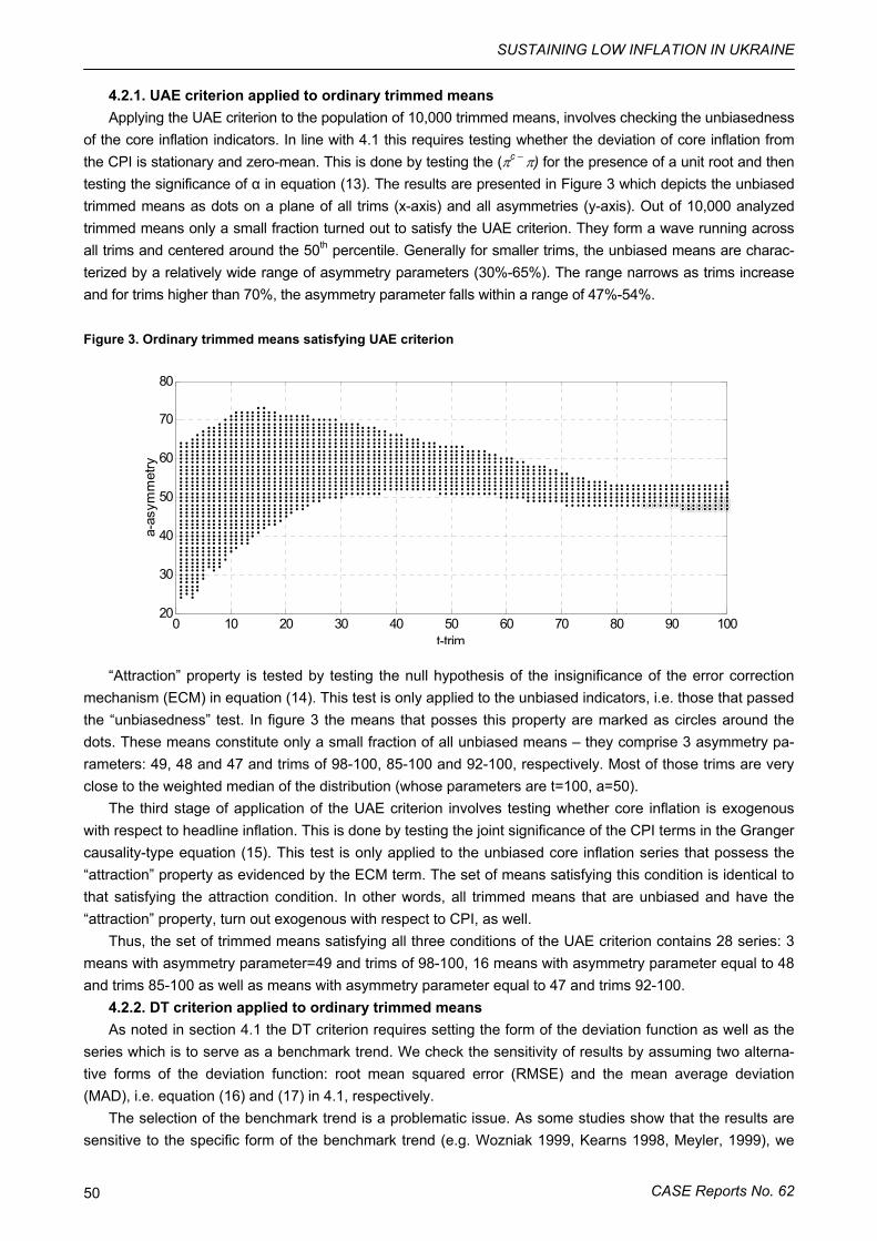
SUSTAINING LOW INFLATION IN UKRAINE
CASE Reports No. 62 50
4.2.1. UAE criterion applied to ordinary trimmed means Applying the UAE criterion to the population of 10,000 trimmed means, involves checking the unbiasedness
of the core inflation indicators. In line with 4.1 this requires testing whether the deviation of core inflation from the CPI is stationary and zero-mean. This is done by testing the (πc – π) for the presence of a unit root and then testing the significance of α in equation (13). The results are presented in Figure 3 which depicts the unbiased trimmed means as dots on a plane of all trims (x-axis) and all asymmetries (y-axis). Out of 10,000 analyzed trimmed means only a small fraction turned out to satisfy the UAE criterion. They form a wave running across all trims and centered around the 50th percentile. Generally for smaller trims, the unbiased means are charac-terized by a relatively wide range of asymmetry parameters (30%-65%). The range narrows as trims increase and for trims higher than 70%, the asymmetry parameter falls within a range of 47%-54%.
Figure 3. Ordinary trimmed means satisfying UAE criterion
0 10 20 30 40 50 60 70 80 90 10020
30
40
50
60
70
80
a-as
ymm
etry
t-trim
“Attraction” property is tested by testing the null hypothesis of the insignificance of the error correction mechanism (ECM) in equation (14). This test is only applied to the unbiased indicators, i.e. those that passed the “unbiasedness” test. In figure 3 the means that posses this property are marked as circles around the dots. These means constitute only a small fraction of all unbiased means – they comprise 3 asymmetry pa-rameters: 49, 48 and 47 and trims of 98-100, 85-100 and 92-100, respectively. Most of those trims are very close to the weighted median of the distribution (whose parameters are t=100, a=50).
The third stage of application of the UAE criterion involves testing whether core inflation is exogenous with respect to headline inflation. This is done by testing the joint significance of the CPI terms in the Granger causality-type equation (15). This test is only applied to the unbiased core inflation series that possess the “attraction” property as evidenced by the ECM term. The set of means satisfying this condition is identical to that satisfying the attraction condition. In other words, all trimmed means that are unbiased and have the “attraction” property, turn out exogenous with respect to CPI, as well.
Thus, the set of trimmed means satisfying all three conditions of the UAE criterion contains 28 series: 3 means with asymmetry parameter=49 and trims of 98-100, 16 means with asymmetry parameter equal to 48 and trims 85-100 as well as means with asymmetry parameter equal to 47 and trims 92-100.
4.2.2. DT criterion applied to ordinary trimmed means As noted in section 4.1 the DT criterion requires setting the form of the deviation function as well as the
series which is to serve as a benchmark trend. We check the sensitivity of results by assuming two alterna-tive forms of the deviation function: root mean squared error (RMSE) and the mean average deviation (MAD), i.e. equation (16) and (17) in 4.1, respectively.
The selection of the benchmark trend is a problematic issue. As some studies show that the results are sensitive to the specific form of the benchmark trend (e.g. Wozniak 1999, Kearns 1998, Meyler, 1999), we
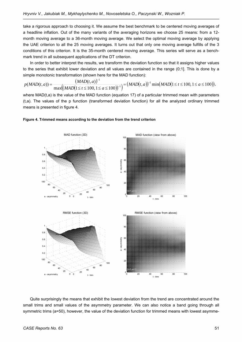
Hryvniv V., Jakubiak M., Mykhaylychenko M., Novoseletska O., Paczynski W., Wozniak P.
CASE Reports No. 63 51
take a rigorous approach to choosing it. We assume the best benchmark to be centered moving averages of a headline inflation. Out of the many variants of the averaging horizons we choose 25 means: from a 12-month moving average to a 36-month moving average. We select the optimal moving average by applying the UAE criterion to all the 25 moving averages. It turns out that only one moving average fulfills of the 3 conditions of this criterion. It is the 35-month centered moving average. This series will serve as a bench-mark trend in all subsequent applications of the DT criterion.
In order to better interpret the results, we transform the deviation function so that it assigns higher values to the series that exhibit lower deviation and all values are contained in the range (0;1]. This is done by a simple monotonic transformation (shown here for the MAD function):
( )( )( )( ) ( )( ) ( )( )1001,1001min,
1001,1001max),()),(( 1
1
1
≤≤≤≤=≤≤≤≤
= −−
−
atMADatMADatMAD
atMADatMADp ,
where MAD(t,a) is the value of the MAD function (equation 17) of a particular trimmed mean with parameters (t,a). The values of the p function (transformed deviation function) for all the analyzed ordinary trimmed means is presented in figure 4.
Figure 4. Trimmed means according to the deviation from the trend criterion
020
4060
80100
020
4060
80100
0.2
0.4
0.6
0.8
1
t - trim
MAD function (3D)
a - asymmetry 0 20 40 60 80 1000
20
40
60
80
100
t - trim
MAD function (view from above)
a - a
sym
met
ry
020
4060
80100
020
4060
80100
0.2
0.4
0.6
0.8
1
t - trim
RMSE function (3D)
a - asymmetry 0 20 40 60 80 1000
20
40
60
80
100
t - trim
RMSE function (view from above)
a - a
sym
met
ry
[t=1,a=1]
[t=1,a=1]
Quite surprisingly the means that exhibit the lowest deviation from the trend are concentrated around the small trims and small values of the asymmetry parameter. We can also notice a band going through all symmetric trims (a=50), however, the value of the deviation function for trimmed means with lowest asymme-
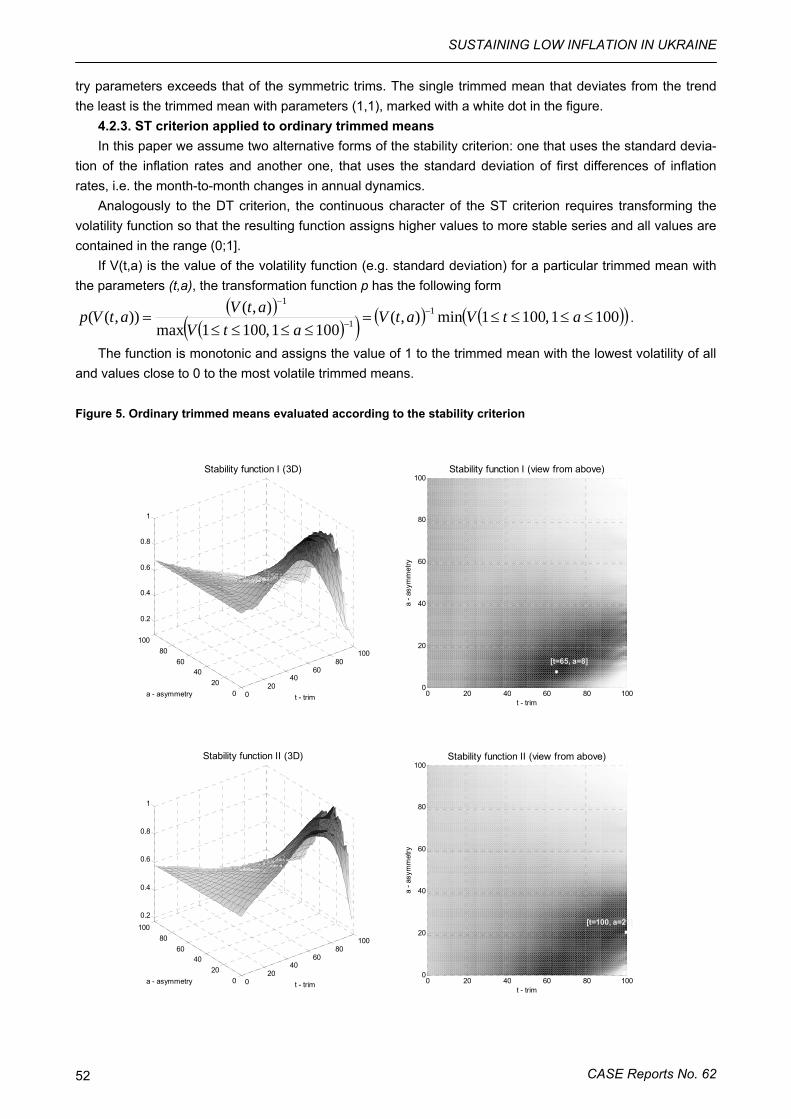
SUSTAINING LOW INFLATION IN UKRAINE
CASE Reports No. 62 52
try parameters exceeds that of the symmetric trims. The single trimmed mean that deviates from the trend the least is the trimmed mean with parameters (1,1), marked with a white dot in the figure.
4.2.3. ST criterion applied to ordinary trimmed means In this paper we assume two alternative forms of the stability criterion: one that uses the standard devia-
tion of the inflation rates and another one, that uses the standard deviation of first differences of inflation rates, i.e. the month-to-month changes in annual dynamics.
Analogously to the DT criterion, the continuous character of the ST criterion requires transforming the volatility function so that the resulting function assigns higher values to more stable series and all values are contained in the range (0;1].
If V(t,a) is the value of the volatility function (e.g. standard deviation) for a particular trimmed mean with the parameters (t,a), the transformation function p has the following form
( )( )( ) ( ) ( )( )1001,1001min),(
1001,1001max),()),(( 1
1
1
≤≤≤≤=≤≤≤≤
= −−
−
atVatVatV
atVatVp .
The function is monotonic and assigns the value of 1 to the trimmed mean with the lowest volatility of all and values close to 0 to the most volatile trimmed means.
Figure 5. Ordinary trimmed means evaluated according to the stability criterion
020
4060
80100
020
4060
80100
0.2
0.4
0.6
0.8
1
t - trim
Stability function I (3D)
a - asymmetry 0 20 40 60 80 1000
20
40
60
80
100
t - trim
Stability function I (view from above)
a - a
sym
met
ry
020
4060
80100
020
4060
80100
0.2
0.4
0.6
0.8
1
t - trim
Stability function II (3D)
a - asymmetry 0 20 40 60 80 1000
20
40
60
80
100
t - trim
Stability function II (view from above)
a - a
sym
met
ry
[t=65, a=8]
[t=100, a=21]
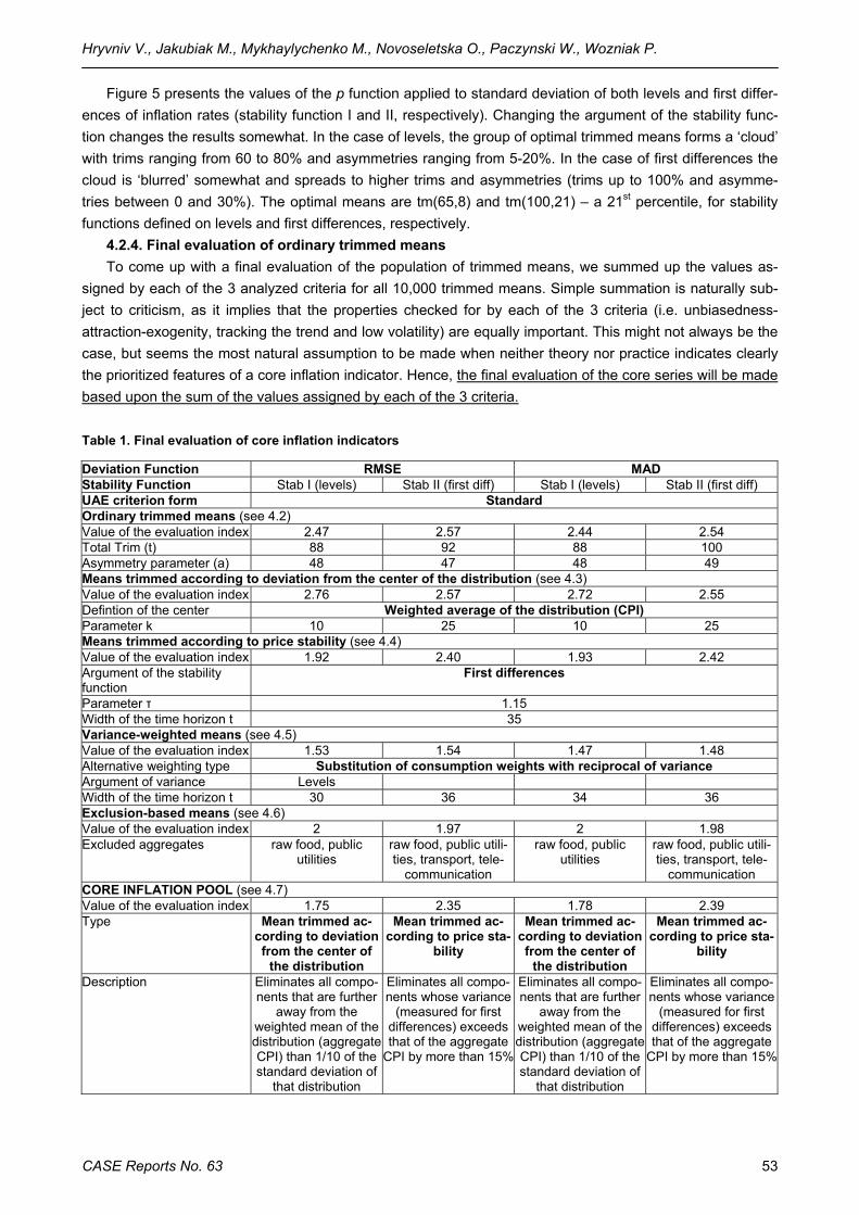
Hryvniv V., Jakubiak M., Mykhaylychenko M., Novoseletska O., Paczynski W., Wozniak P.
CASE Reports No. 63 53
Figure 5 presents the values of the p function applied to standard deviation of both levels and first differ-ences of inflation rates (stability function I and II, respectively). Changing the argument of the stability func-tion changes the results somewhat. In the case of levels, the group of optimal trimmed means forms a ‘cloud’ with trims ranging from 60 to 80% and asymmetries ranging from 5-20%. In the case of first differences the cloud is ‘blurred’ somewhat and spreads to higher trims and asymmetries (trims up to 100% and asymme-tries between 0 and 30%). The optimal means are tm(65,8) and tm(100,21) – a 21st percentile, for stability functions defined on levels and first differences, respectively.
4.2.4. Final evaluation of ordinary trimmed means To come up with a final evaluation of the population of trimmed means, we summed up the values as-
signed by each of the 3 analyzed criteria for all 10,000 trimmed means. Simple summation is naturally sub-ject to criticism, as it implies that the properties checked for by each of the 3 criteria (i.e. unbiasedness-attraction-exogenity, tracking the trend and low volatility) are equally important. This might not always be the case, but seems the most natural assumption to be made when neither theory nor practice indicates clearly the prioritized features of a core inflation indicator. Hence, the final evaluation of the core series will be made based upon the sum of the values assigned by each of the 3 criteria.
Table 1. Final evaluation of core inflation indicators
Deviation Function RMSE MAD Stability Function Stab I (levels) Stab II (first diff) Stab I (levels) Stab II (first diff) UAE criterion form Standard Ordinary trimmed means (see 4.2) Value of the evaluation index 2.47 2.57 2.44 2.54 Total Trim (t) 88 92 88 100 Asymmetry parameter (a) 48 47 48 49 Means trimmed according to deviation from the center of the distribution (see 4.3) Value of the evaluation index 2.76 2.57 2.72 2.55 Defintion of the center Weighted average of the distribution (CPI) Parameter k 10 25 10 25 Means trimmed according to price stability (see 4.4) Value of the evaluation index 1.92 2.40 1.93 2.42 Argument of the stability function
First differences
Parameter τ 1.15 Width of the time horizon t 35 Variance-weighted means (see 4.5) Value of the evaluation index 1.53 1.54 1.47 1.48 Alternative weighting type Substitution of consumption weights with reciprocal of variance Argument of variance Levels Width of the time horizon t 30 36 34 36 Exclusion-based means (see 4.6) Value of the evaluation index 2 1.97 2 1.98 Excluded aggregates raw food, public
utilities raw food, public utili-ties, transport, tele-
communication
raw food, public utilities
raw food, public utili-ties, transport, tele-
communication CORE INFLATION POOL (see 4.7) Value of the evaluation index 1.75 2.35 1.78 2.39 Type Mean trimmed ac-
cording to deviation from the center of
the distribution
Mean trimmed ac-cording to price sta-
bility
Mean trimmed ac-cording to deviation from the center of
the distribution
Mean trimmed ac-cording to price sta-
bility
Description Eliminates all compo-nents that are further
away from the weighted mean of the distribution (aggregate CPI) than 1/10 of the standard deviation of
that distribution
Eliminates all compo-nents whose variance
(measured for first differences) exceeds that of the aggregate
CPI by more than 15%
Eliminates all compo-nents that are further
away from the weighted mean of the distribution (aggregate CPI) than 1/10 of the standard deviation of
that distribution
Eliminates all compo-nents whose variance
(measured for first differences) exceeds that of the aggregate
CPI by more than 15%
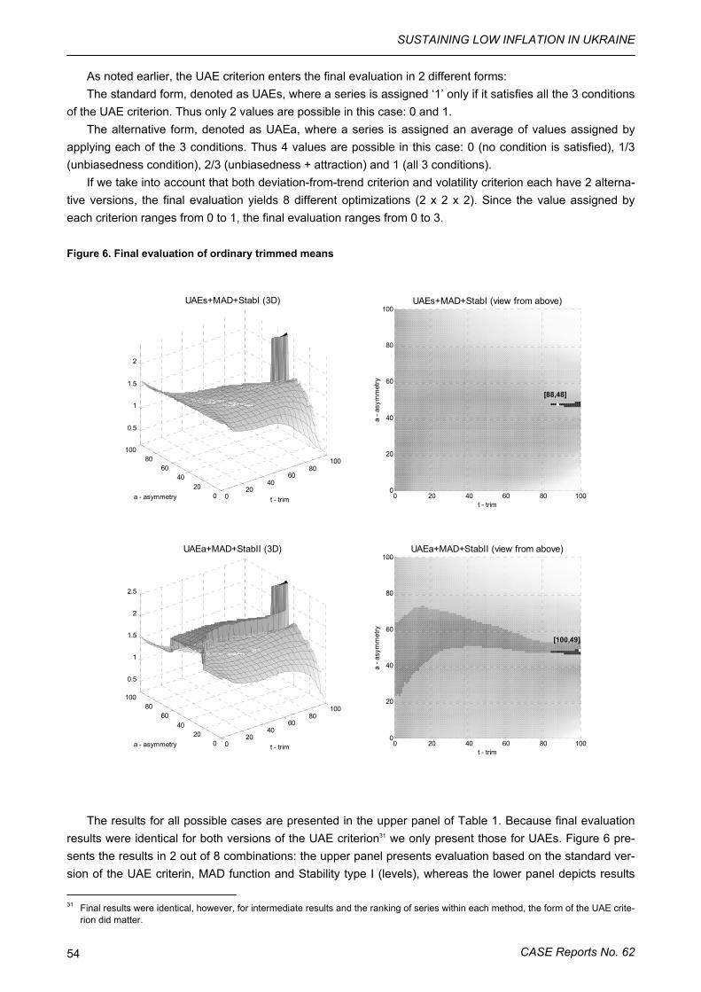
SUSTAINING LOW INFLATION IN UKRAINE
CASE Reports No. 62 54
As noted earlier, the UAE criterion enters the final evaluation in 2 different forms: The standard form, denoted as UAEs, where a series is assigned ‘1’ only if it satisfies all the 3 conditions
of the UAE criterion. Thus only 2 values are possible in this case: 0 and 1. The alternative form, denoted as UAEa, where a series is assigned an average of values assigned by
applying each of the 3 conditions. Thus 4 values are possible in this case: 0 (no condition is satisfied), 1/3 (unbiasedness condition), 2/3 (unbiasedness + attraction) and 1 (all 3 conditions).
If we take into account that both deviation-from-trend criterion and volatility criterion each have 2 alterna-tive versions, the final evaluation yields 8 different optimizations (2 x 2 x 2). Since the value assigned by each criterion ranges from 0 to 1, the final evaluation ranges from 0 to 3.
Figure 6. Final evaluation of ordinary trimmed means
020
4060
80100
020
4060
80100
0.5
1
1.5
2
t - trim
UAEs+MAD+StabI (3D)
a - asymmetry 0 20 40 60 80 1000
20
40
60
80
100
t - trim
UAEs+MAD+StabI (view from above)
a - a
sym
met
ry
020
4060
80100
020
4060
80100
0.5
1
1.5
2
2.5
t - trim
UAEa+MAD+StabII (3D)
a - asymmetry 0 20 40 60 80 1000
20
40
60
80
100
t - trim
UAEa+MAD+StabII (view from above)
a - a
sym
met
ry
[88,48]
[100,49]
The results for all possible cases are presented in the upper panel of Table 1. Because final evaluation results were identical for both versions of the UAE criterion31 we only present those for UAEs. Figure 6 pre-sents the results in 2 out of 8 combinations: the upper panel presents evaluation based on the standard ver-sion of the UAE criterin, MAD function and Stability type I (levels), whereas the lower panel depicts results
31 Final results were identical, however, for intermediate results and the ranking of series within each method, the form of the UAE crite-
rion did matter.
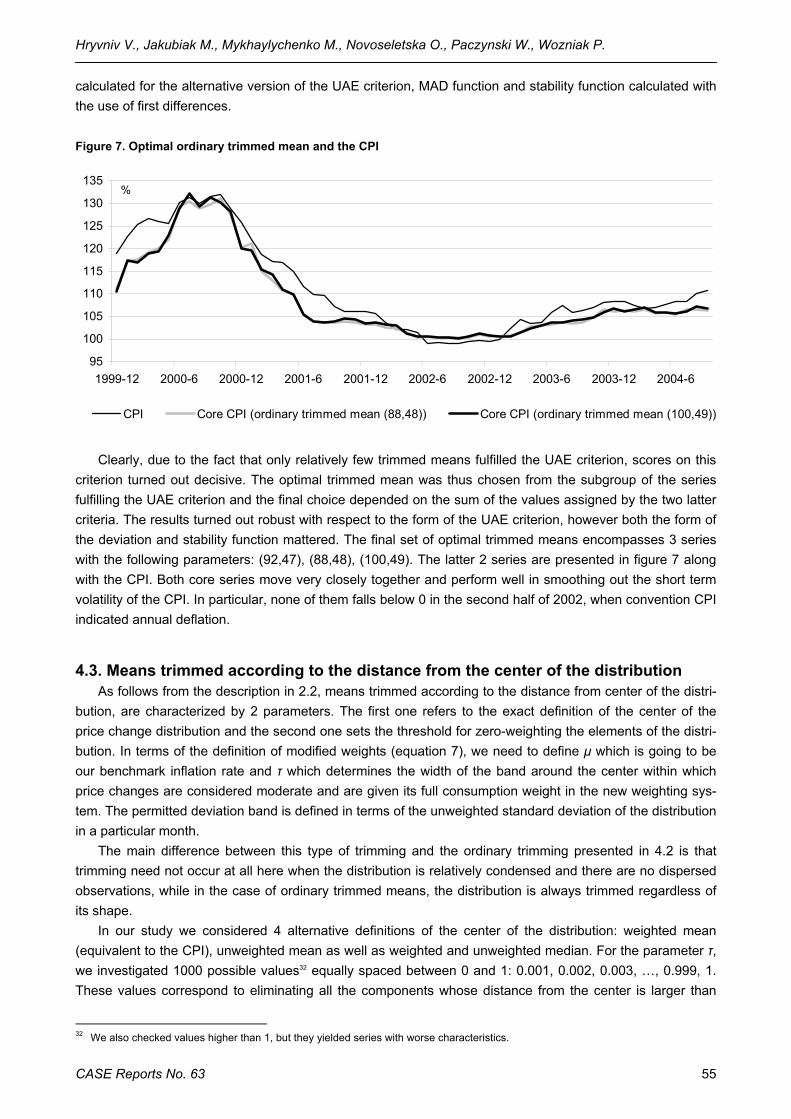
Hryvniv V., Jakubiak M., Mykhaylychenko M., Novoseletska O., Paczynski W., Wozniak P.
CASE Reports No. 63 55
calculated for the alternative version of the UAE criterion, MAD function and stability function calculated with the use of first differences.
Figure 7. Optimal ordinary trimmed mean and the CPI
95
100
105
110
115
120
125
130
135
1999-12 2000-6 2000-12 2001-6 2001-12 2002-6 2002-12 2003-6 2003-12 2004-6
CPI Core CPI (ordinary trimmed mean (88,48)) Core CPI (ordinary trimmed mean (100,49))
%
Clearly, due to the fact that only relatively few trimmed means fulfilled the UAE criterion, scores on this criterion turned out decisive. The optimal trimmed mean was thus chosen from the subgroup of the series fulfilling the UAE criterion and the final choice depended on the sum of the values assigned by the two latter criteria. The results turned out robust with respect to the form of the UAE criterion, however both the form of the deviation and stability function mattered. The final set of optimal trimmed means encompasses 3 series with the following parameters: (92,47), (88,48), (100,49). The latter 2 series are presented in figure 7 along with the CPI. Both core series move very closely together and perform well in smoothing out the short term volatility of the CPI. In particular, none of them falls below 0 in the second half of 2002, when convention CPI indicated annual deflation.
4.3. Means trimmed according to the distance from the center of the distribution As follows from the description in 2.2, means trimmed according to the distance from center of the distri-
bution, are characterized by 2 parameters. The first one refers to the exact definition of the center of the price change distribution and the second one sets the threshold for zero-weighting the elements of the distri-bution. In terms of the definition of modified weights (equation 7), we need to define μ which is going to be our benchmark inflation rate and τ which determines the width of the band around the center within which price changes are considered moderate and are given its full consumption weight in the new weighting sys-tem. The permitted deviation band is defined in terms of the unweighted standard deviation of the distribution in a particular month.
The main difference between this type of trimming and the ordinary trimming presented in 4.2 is that trimming need not occur at all here when the distribution is relatively condensed and there are no dispersed observations, while in the case of ordinary trimmed means, the distribution is always trimmed regardless of its shape.
In our study we considered 4 alternative definitions of the center of the distribution: weighted mean (equivalent to the CPI), unweighted mean as well as weighted and unweighted median. For the parameter τ, we investigated 1000 possible values32 equally spaced between 0 and 1: 0.001, 0.002, 0.003, …, 0.999, 1. These values correspond to eliminating all the components whose distance from the center is larger than
32 We also checked values higher than 1, but they yielded series with worse characteristics.

SUSTAINING LOW INFLATION IN UKRAINE
CASE Reports No. 62 56
1/1000 of a standard deviation up to eliminating all the components further away from the center than 1 standard deviation. Accordingly, the population of means trimmed according to this method is 4000 (4 defini-tions of μ times 1000 values for τ)
The analysis will proceed analogously to that in the preceding subsection. Unlike in the previous case, however, we will not present all the intermediate results and instead we will focus on the final evaluation. Table 1 presents full results of the evaluation procedure for possible combinations of alternative criteria, while figure 8 presents the evaluation score of each of the 400 means in 2 chosen cases. As table 1 sug-gests, in all cases, the optimal series are centered around the weighted mean, i.e. the CPI (μ1), means cal-culated with the use of other definitions of the center of the distribution scored visibly worse. Furthermore, the results turned out robust with respect to the deviation function (criterion DT) and the form of the UAE cri-terion. However, as was the case with ordinary trimmed means, the form of the stability function determines the specific final result. When we evaluate means according to stability function calculated on levels, the op-timal series is the mean with paramter τ=0.1 while, if the function’s arguments are first difference, the optimal mean is characterized by parameter τ=0.25.
Figure 8. Final evaluation of means trimmed according to the distance from the center of the distribution
1.01.21.41.61.82.02.22.42.62.8
0.01
0.04
0.07
0.10
0.13
0.16
0.19
0.22
0.25
0.28
0.31
0.34
0.37
0.40
0.43
0.46
0.49
0.52
0.55
0.58
0.61
0.64
0.67
0.70
0.73
0.76
0.79
0.82
0.85
0.88
0.91
0.94
0.97
1.00
μ1 -weighted mean μ2 -weighted medianμ3 -unweighted mean μ4 -unweighted median
τ
STABILITY function calculated on levels; RMSE; UAEaτ = 0.246
1.01.21.41.61.82.02.22.42.62.8
0.01
0.04
0.07
0.10
0.13
0.16
0.19
0.22
0.25
0.28
0.31
0.34
0.37
0.40
0.43
0.46
0.49
0.52
0.55
0.58
0.61
0.64
0.67
0.70
0.73
0.76
0.79
0.82
0.85
0.88
0.91
0.94
0.97
1.00
μ1 -weighted mean μ2 -weighted medianμ3 -unweighted mean μ4 -unweighted median
τ
STABILITY function calculated on first differences; MAD; UAEaτ = 0.097
The figure graphs four lines (each for an alternative definition of the distribution center) as a function of the τ parameter. Because the form of the stability function used mattered for results, figure 8 contains two graphs: the upper one for the evaluation with the use of the stability function calculated on levels (Stab I) and the lower one plotting the results obtained with the use of the stability function calculated on first differences
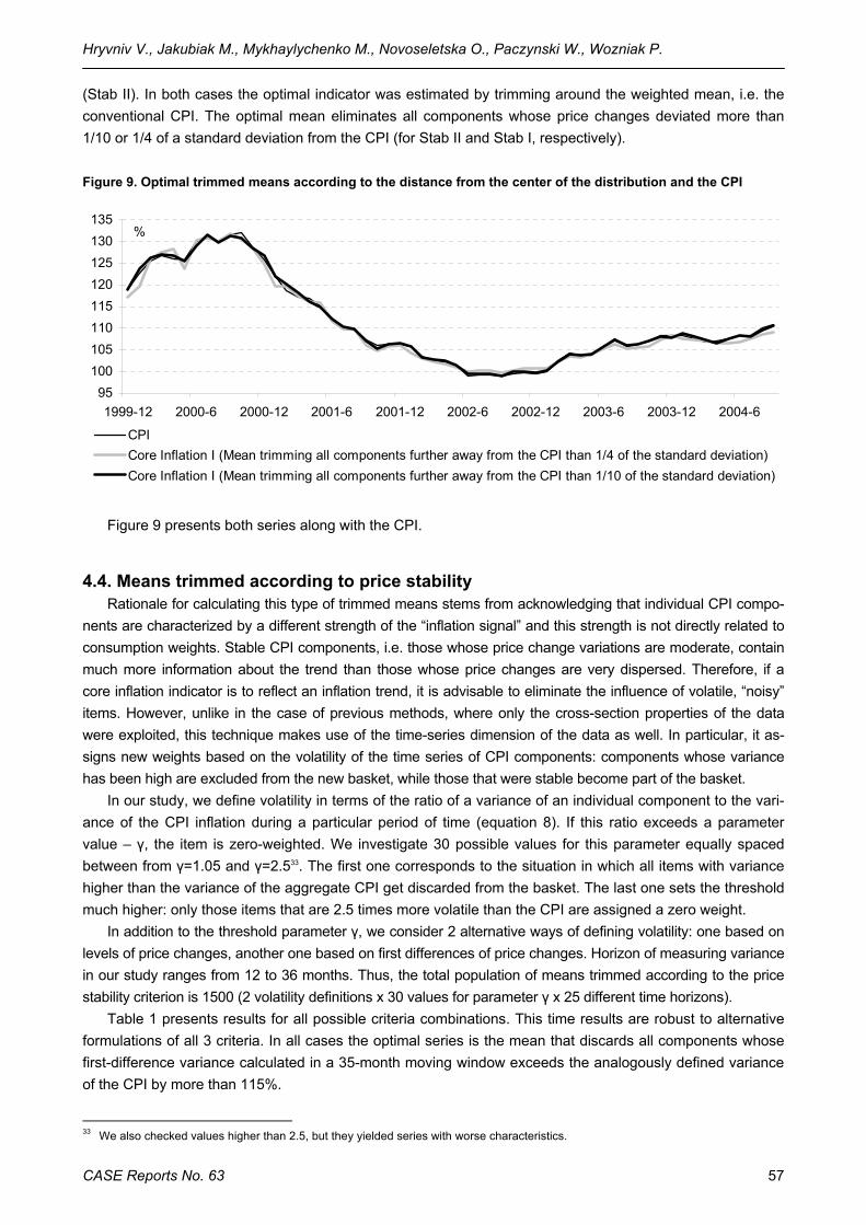
Hryvniv V., Jakubiak M., Mykhaylychenko M., Novoseletska O., Paczynski W., Wozniak P.
CASE Reports No. 63 57
(Stab II). In both cases the optimal indicator was estimated by trimming around the weighted mean, i.e. the conventional CPI. The optimal mean eliminates all components whose price changes deviated more than 1/10 or 1/4 of a standard deviation from the CPI (for Stab II and Stab I, respectively).
Figure 9. Optimal trimmed means according to the distance from the center of the distribution and the CPI
95100105110115120125130135
1999-12 2000-6 2000-12 2001-6 2001-12 2002-6 2002-12 2003-6 2003-12 2004-6
CPICore Inflation I (Mean trimming all components further away from the CPI than 1/4 of the standard deviation)Core Inflation I (Mean trimming all components further away from the CPI than 1/10 of the standard deviation)
%
Figure 9 presents both series along with the CPI.
4.4. Means trimmed according to price stability Rationale for calculating this type of trimmed means stems from acknowledging that individual CPI compo-
nents are characterized by a different strength of the “inflation signal” and this strength is not directly related to consumption weights. Stable CPI components, i.e. those whose price change variations are moderate, contain much more information about the trend than those whose price changes are very dispersed. Therefore, if a core inflation indicator is to reflect an inflation trend, it is advisable to eliminate the influence of volatile, “noisy” items. However, unlike in the case of previous methods, where only the cross-section properties of the data were exploited, this technique makes use of the time-series dimension of the data as well. In particular, it as-signs new weights based on the volatility of the time series of CPI components: components whose variance has been high are excluded from the new basket, while those that were stable become part of the basket.
In our study, we define volatility in terms of the ratio of a variance of an individual component to the vari-ance of the CPI inflation during a particular period of time (equation 8). If this ratio exceeds a parameter value – γ, the item is zero-weighted. We investigate 30 possible values for this parameter equally spaced between from γ=1.05 and γ=2.533. The first one corresponds to the situation in which all items with variance higher than the variance of the aggregate CPI get discarded from the basket. The last one sets the threshold much higher: only those items that are 2.5 times more volatile than the CPI are assigned a zero weight.
In addition to the threshold parameter γ, we consider 2 alternative ways of defining volatility: one based on levels of price changes, another one based on first differences of price changes. Horizon of measuring variance in our study ranges from 12 to 36 months. Thus, the total population of means trimmed according to the price stability criterion is 1500 (2 volatility definitions x 30 values for parameter γ x 25 different time horizons).
Table 1 presents results for all possible criteria combinations. This time results are robust to alternative formulations of all 3 criteria. In all cases the optimal series is the mean that discards all components whose first-difference variance calculated in a 35-month moving window exceeds the analogously defined variance of the CPI by more than 115%.
33 We also checked values higher than 2.5, but they yielded series with worse characteristics.
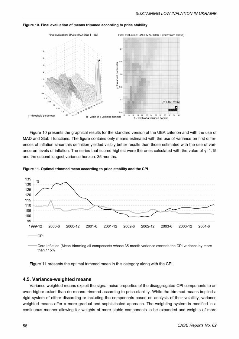
SUSTAINING LOW INFLATION IN UKRAINE
CASE Reports No. 62 58
Figure 10. Final evaluation of means trimmed according to price stability
1214 16
1820
2224
2628
30 3234
1.05
1.3
1.55
1.8
2.05
2.3
0.8
1
1.2
1.4
1.6
1.8
2
h - width of a variance horizon
Final evaluation: UAEs;MAD;Stab I (3D)
γ - threshold parameter 12 14 16 18 20 22 24 26 28 30 32 34 361.05
1.3
1.55
1.8
2.05
2.3
[γ= 1.15 ; h=35]
h - width of a variance horizon
Final evaluation: UAEs;MAD;Stab I (view from above)
γ - th
resh
old
para
met
er
Figure 10 presents the graphical results for the standard version of the UEA criterion and with the use of MAD and Stab I functions. The figure contains only means estimated with the use of variance on first differ-ences of inflation since this definition yielded visibly better results than those estimated with the use of vari-ance on levels of inflation. The series that scored highest were the ones calculated with the value of γ=1.15 and the second longest variance horizon: 35 months.
Figure 11. Optimal trimmed mean according to price stability and the CPI
95100105110115120125130135
1999-12 2000-6 2000-12 2001-6 2001-12 2002-6 2002-12 2003-6 2003-12 2004-6
CPI
Core Inflation (Mean trimming all components whose 35-month variance exceeds the CPI variance by morethan 115%
%
Figure 11 presents the optimal trimmed mean in this category along with the CPI.
4.5. Variance-weighted means Variance weighted means exploit the signal-noise properties of the disaggregated CPI components to an
even higher extent than do means trimmed according to price stability. While the trimmed means implied a rigid system of either discarding or including the components based on analysis of their volatility, variance weighted means offer a more gradual and sophisticated approach. The weighting system is modified in a continuous manner allowing for weights of more stable components to be expanded and weights of more
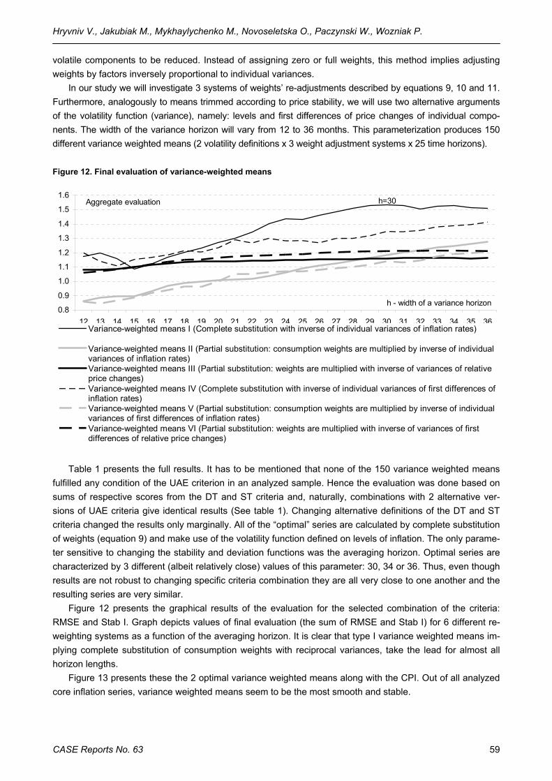
Hryvniv V., Jakubiak M., Mykhaylychenko M., Novoseletska O., Paczynski W., Wozniak P.
CASE Reports No. 63 59
volatile components to be reduced. Instead of assigning zero or full weights, this method implies adjusting weights by factors inversely proportional to individual variances.
In our study we will investigate 3 systems of weights’ re-adjustments described by equations 9, 10 and 11. Furthermore, analogously to means trimmed according to price stability, we will use two alternative arguments of the volatility function (variance), namely: levels and first differences of price changes of individual compo-nents. The width of the variance horizon will vary from 12 to 36 months. This parameterization produces 150 different variance weighted means (2 volatility definitions x 3 weight adjustment systems x 25 time horizons).
Figure 12. Final evaluation of variance-weighted means
0.8
0.9
1.0
1.1
1.2
1.3
1.4
1.5
1.6
12 13 14 15 16 17 18 19 20 21 22 23 24 25 26 27 28 29 30 31 32 33 34 35 36
h - width of a variance horizon
Aggregate evaluation
Variance-weighted means I (Complete substitution with inverse of individual variances of inflation rates)
Variance-weighted means II (Partial substitution: consumption weights are multiplied by inverse of individualvariances of inflation rates)Variance-weighted means III (Partial substitution: weights are multiplied with inverse of variances of relativeprice changes)Variance-weighted means IV (Complete substitution with inverse of individual variances of first differences ofinflation rates)Variance-weighted means V (Partial substitution: consumption weights are multiplied by inverse of individualvariances of first differences of inflation rates)Variance-weighted means VI (Partial substitution: weights are multiplied with inverse of variances of firstdifferences of relative price changes)
h=30
Table 1 presents the full results. It has to be mentioned that none of the 150 variance weighted means fulfilled any condition of the UAE criterion in an analyzed sample. Hence the evaluation was done based on sums of respective scores from the DT and ST criteria and, naturally, combinations with 2 alternative ver-sions of UAE criteria give identical results (See table 1). Changing alternative definitions of the DT and ST criteria changed the results only marginally. All of the “optimal” series are calculated by complete substitution of weights (equation 9) and make use of the volatility function defined on levels of inflation. The only parame-ter sensitive to changing the stability and deviation functions was the averaging horizon. Optimal series are characterized by 3 different (albeit relatively close) values of this parameter: 30, 34 or 36. Thus, even though results are not robust to changing specific criteria combination they are all very close to one another and the resulting series are very similar.
Figure 12 presents the graphical results of the evaluation for the selected combination of the criteria: RMSE and Stab I. Graph depicts values of final evaluation (the sum of RMSE and Stab I) for 6 different re-weighting systems as a function of the averaging horizon. It is clear that type I variance weighted means im-plying complete substitution of consumption weights with reciprocal variances, take the lead for almost all horizon lengths.
Figure 13 presents these the 2 optimal variance weighted means along with the CPI. Out of all analyzed core inflation series, variance weighted means seem to be the most smooth and stable.
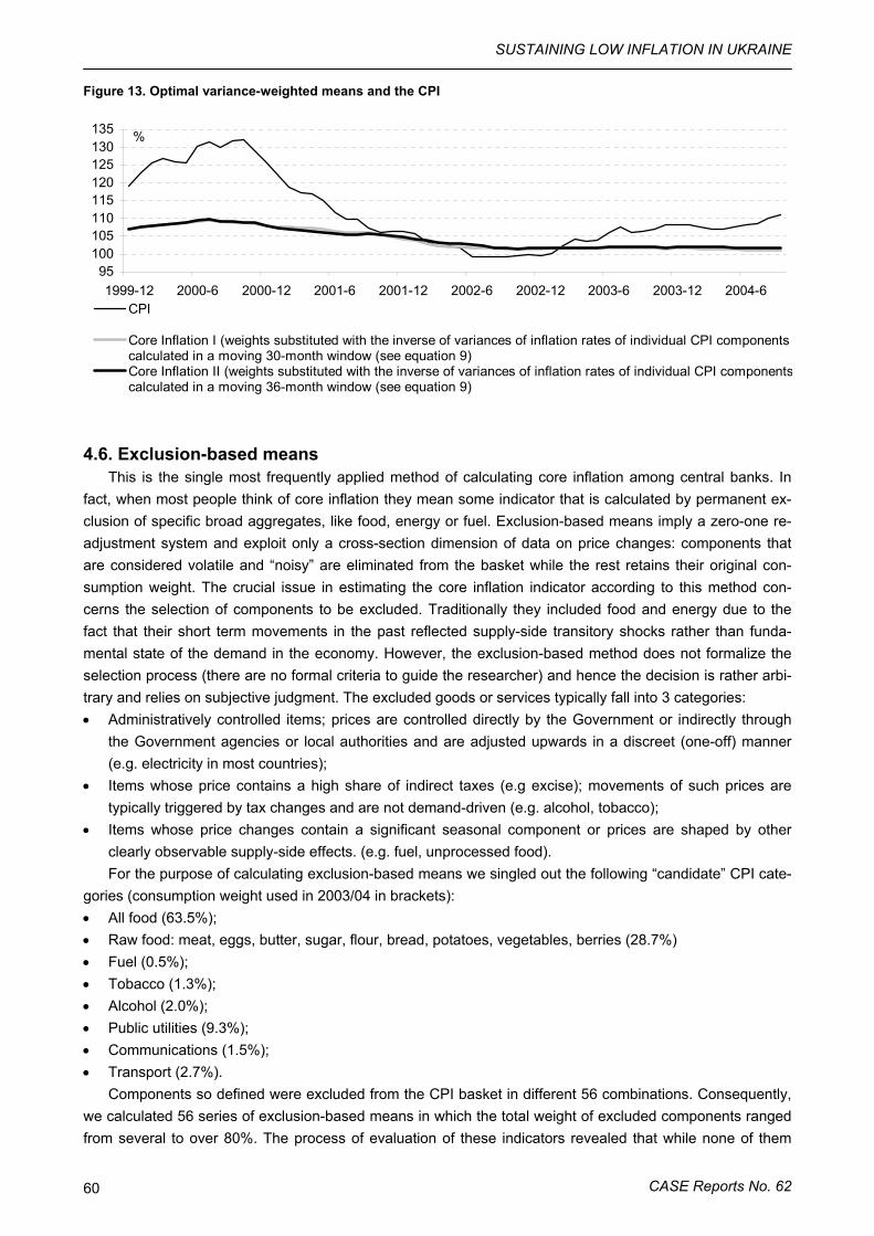
SUSTAINING LOW INFLATION IN UKRAINE
CASE Reports No. 62 60
Figure 13. Optimal variance-weighted means and the CPI
95100105110115120125130135
1999-12 2000-6 2000-12 2001-6 2001-12 2002-6 2002-12 2003-6 2003-12 2004-6CPI
Core Inflation I (weights substituted with the inverse of variances of inflation rates of individual CPI componentscalculated in a moving 30-month window (see equation 9)Core Inflation II (weights substituted with the inverse of variances of inflation rates of individual CPI componentscalculated in a moving 36-month window (see equation 9)
%
4.6. Exclusion-based means This is the single most frequently applied method of calculating core inflation among central banks. In
fact, when most people think of core inflation they mean some indicator that is calculated by permanent ex-clusion of specific broad aggregates, like food, energy or fuel. Exclusion-based means imply a zero-one re-adjustment system and exploit only a cross-section dimension of data on price changes: components that are considered volatile and “noisy” are eliminated from the basket while the rest retains their original con-sumption weight. The crucial issue in estimating the core inflation indicator according to this method con-cerns the selection of components to be excluded. Traditionally they included food and energy due to the fact that their short term movements in the past reflected supply-side transitory shocks rather than funda-mental state of the demand in the economy. However, the exclusion-based method does not formalize the selection process (there are no formal criteria to guide the researcher) and hence the decision is rather arbi-trary and relies on subjective judgment. The excluded goods or services typically fall into 3 categories: • Administratively controlled items; prices are controlled directly by the Government or indirectly through
the Government agencies or local authorities and are adjusted upwards in a discreet (one-off) manner (e.g. electricity in most countries);
• Items whose price contains a high share of indirect taxes (e.g excise); movements of such prices are typically triggered by tax changes and are not demand-driven (e.g. alcohol, tobacco);
• Items whose price changes contain a significant seasonal component or prices are shaped by other clearly observable supply-side effects. (e.g. fuel, unprocessed food). For the purpose of calculating exclusion-based means we singled out the following “candidate” CPI cate-
gories (consumption weight used in 2003/04 in brackets): • All food (63.5%); • Raw food: meat, eggs, butter, sugar, flour, bread, potatoes, vegetables, berries (28.7%) • Fuel (0.5%); • Tobacco (1.3%); • Alcohol (2.0%); • Public utilities (9.3%); • Communications (1.5%); • Transport (2.7%).
Components so defined were excluded from the CPI basket in different 56 combinations. Consequently, we calculated 56 series of exclusion-based means in which the total weight of excluded components ranged from several to over 80%. The process of evaluation of these indicators revealed that while none of them
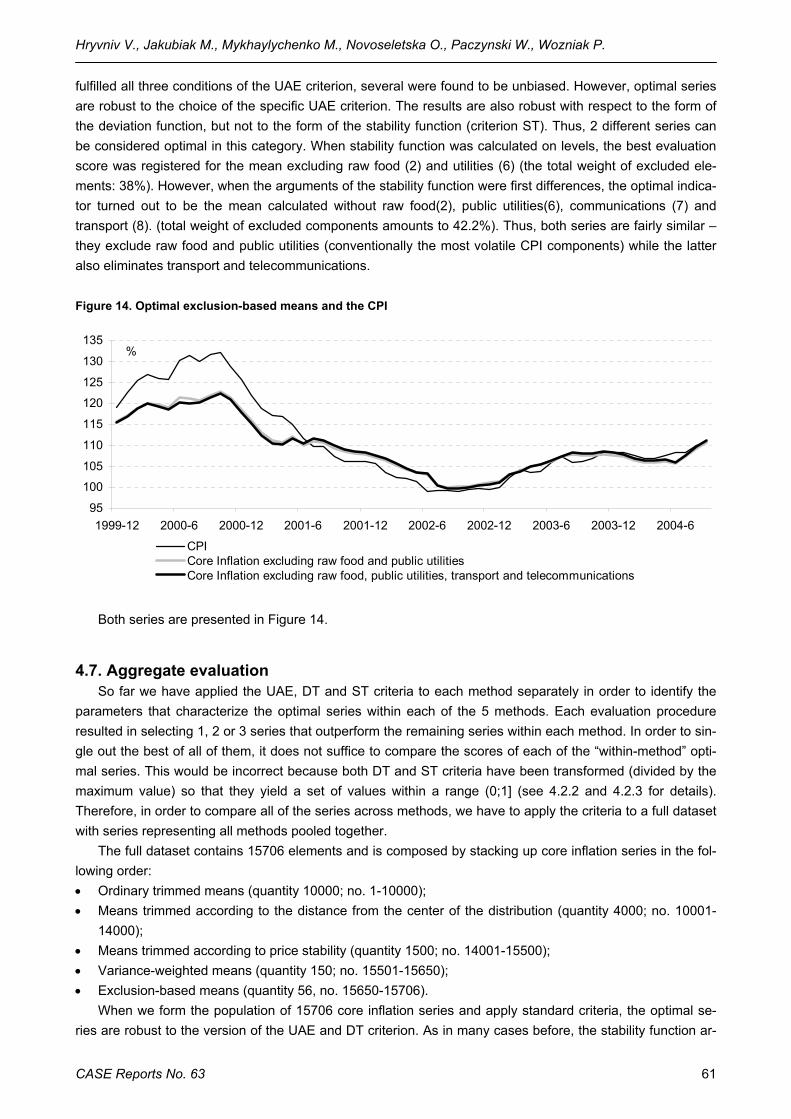
Hryvniv V., Jakubiak M., Mykhaylychenko M., Novoseletska O., Paczynski W., Wozniak P.
CASE Reports No. 63 61
fulfilled all three conditions of the UAE criterion, several were found to be unbiased. However, optimal series are robust to the choice of the specific UAE criterion. The results are also robust with respect to the form of the deviation function, but not to the form of the stability function (criterion ST). Thus, 2 different series can be considered optimal in this category. When stability function was calculated on levels, the best evaluation score was registered for the mean excluding raw food (2) and utilities (6) (the total weight of excluded ele-ments: 38%). However, when the arguments of the stability function were first differences, the optimal indica-tor turned out to be the mean calculated without raw food(2), public utilities(6), communications (7) and transport (8). (total weight of excluded components amounts to 42.2%). Thus, both series are fairly similar – they exclude raw food and public utilities (conventionally the most volatile CPI components) while the latter also eliminates transport and telecommunications.
Figure 14. Optimal exclusion-based means and the CPI
95
100
105
110
115
120
125
130
135
1999-12 2000-6 2000-12 2001-6 2001-12 2002-6 2002-12 2003-6 2003-12 2004-6
CPICore Inflation excluding raw food and public utilities Core Inflation excluding raw food, public utilities, transport and telecommunications
%
Both series are presented in Figure 14.
4.7. Aggregate evaluation So far we have applied the UAE, DT and ST criteria to each method separately in order to identify the
parameters that characterize the optimal series within each of the 5 methods. Each evaluation procedure resulted in selecting 1, 2 or 3 series that outperform the remaining series within each method. In order to sin-gle out the best of all of them, it does not suffice to compare the scores of each of the “within-method” opti-mal series. This would be incorrect because both DT and ST criteria have been transformed (divided by the maximum value) so that they yield a set of values within a range (0;1] (see 4.2.2 and 4.2.3 for details). Therefore, in order to compare all of the series across methods, we have to apply the criteria to a full dataset with series representing all methods pooled together.
The full dataset contains 15706 elements and is composed by stacking up core inflation series in the fol-lowing order: • Ordinary trimmed means (quantity 10000; no. 1-10000); • Means trimmed according to the distance from the center of the distribution (quantity 4000; no. 10001-
14000); • Means trimmed according to price stability (quantity 1500; no. 14001-15500); • Variance-weighted means (quantity 150; no. 15501-15650); • Exclusion-based means (quantity 56, no. 15650-15706).
When we form the population of 15706 core inflation series and apply standard criteria, the optimal se-ries are robust to the version of the UAE and DT criterion. As in many cases before, the stability function ar-
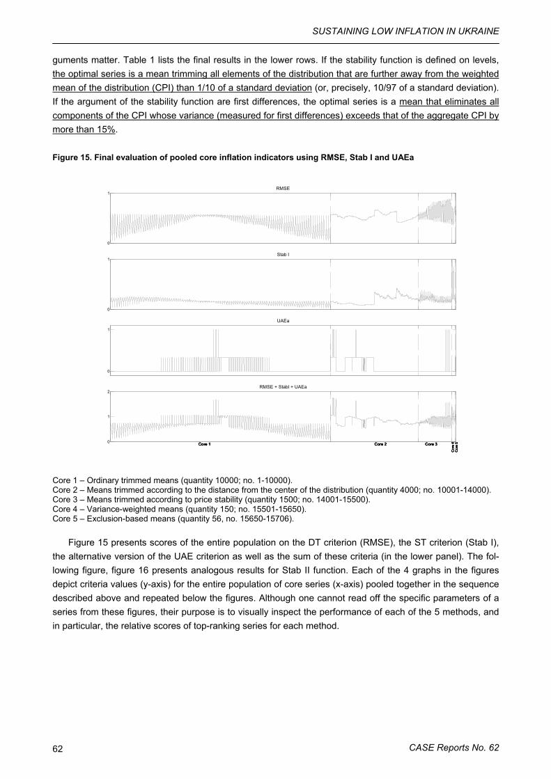
SUSTAINING LOW INFLATION IN UKRAINE
CASE Reports No. 62 62
guments matter. Table 1 lists the final results in the lower rows. If the stability function is defined on levels, the optimal series is a mean trimming all elements of the distribution that are further away from the weighted mean of the distribution (CPI) than 1/10 of a standard deviation (or, precisely, 10/97 of a standard deviation). If the argument of the stability function are first differences, the optimal series is a mean that eliminates all components of the CPI whose variance (measured for first differences) exceeds that of the aggregate CPI by more than 15%.
Figure 15. Final evaluation of pooled core inflation indicators using RMSE, Stab I and UAEa
0
1RMSE
0
1Stab I
0
1
UAEa
0
1
2RMSE + StabI + UAEa
Core 1 Core 2 Core 3
Cor
e 4
Cor
e 5Core 1 Core 2 Core 3
Cor
e 4
Cor
e 5Core 1 Core 2 Core 3
Cor
e 4
Cor
e 5Core 1 Core 2 Core 3
Cor
e 4
Cor
e 5
Core 1 – Ordinary trimmed means (quantity 10000; no. 1-10000). Core 2 – Means trimmed according to the distance from the center of the distribution (quantity 4000; no. 10001-14000). Core 3 – Means trimmed according to price stability (quantity 1500; no. 14001-15500). Core 4 – Variance-weighted means (quantity 150; no. 15501-15650). Core 5 – Exclusion-based means (quantity 56, no. 15650-15706).
Figure 15 presents scores of the entire population on the DT criterion (RMSE), the ST criterion (Stab I), the alternative version of the UAE criterion as well as the sum of these criteria (in the lower panel). The fol-lowing figure, figure 16 presents analogous results for Stab II function. Each of the 4 graphs in the figures depict criteria values (y-axis) for the entire population of core series (x-axis) pooled together in the sequence described above and repeated below the figures. Although one cannot read off the specific parameters of a series from these figures, their purpose is to visually inspect the performance of each of the 5 methods, and in particular, the relative scores of top-ranking series for each method.
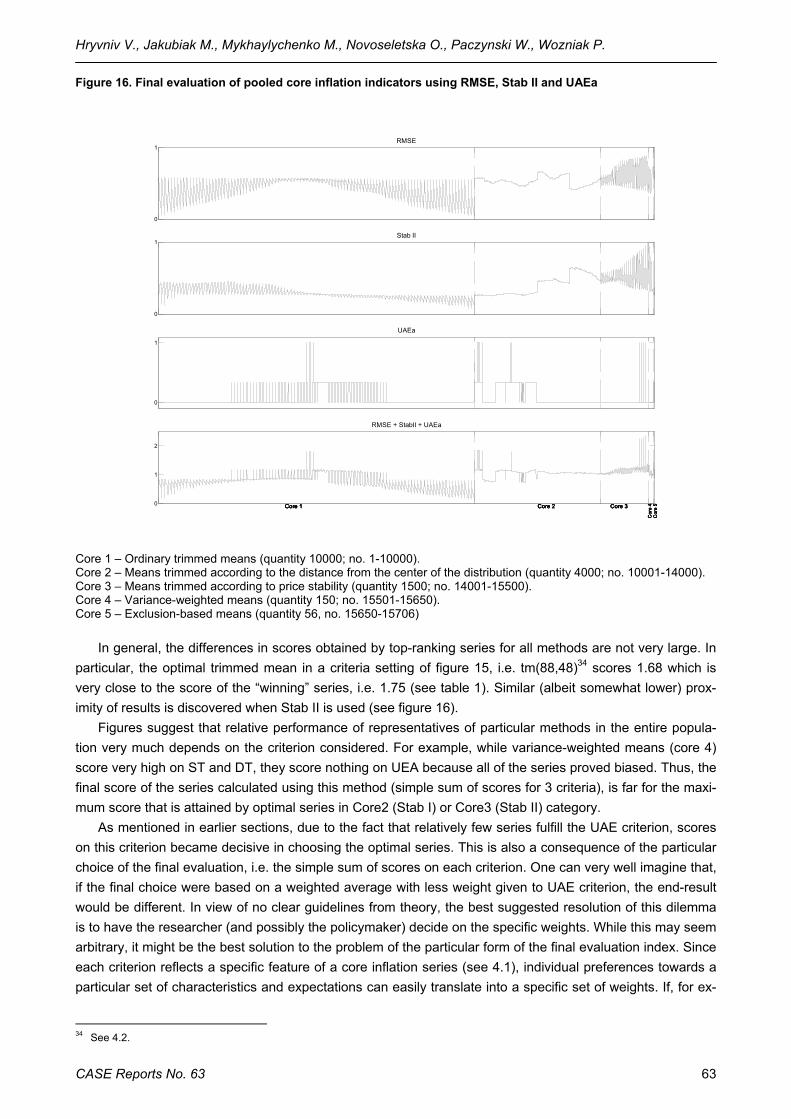
Hryvniv V., Jakubiak M., Mykhaylychenko M., Novoseletska O., Paczynski W., Wozniak P.
CASE Reports No. 63 63
Figure 16. Final evaluation of pooled core inflation indicators using RMSE, Stab II and UAEa
0
1RMSE
0
1Stab II
0
1
UAEa
0
1
2
RMSE + StabII + UAEa
Core 1 Core 2 Core 3
Cor
e 4
Cor
e 5Core 1 Core 2 Core 3
Cor
e 4
Cor
e 5Core 1 Core 2 Core 3
Cor
e 4
Cor
e 5Core 1 Core 2 Core 3
Cor
e 4
Cor
e 5
Core 1 – Ordinary trimmed means (quantity 10000; no. 1-10000). Core 2 – Means trimmed according to the distance from the center of the distribution (quantity 4000; no. 10001-14000). Core 3 – Means trimmed according to price stability (quantity 1500; no. 14001-15500). Core 4 – Variance-weighted means (quantity 150; no. 15501-15650). Core 5 – Exclusion-based means (quantity 56, no. 15650-15706)
In general, the differences in scores obtained by top-ranking series for all methods are not very large. In particular, the optimal trimmed mean in a criteria setting of figure 15, i.e. tm(88,48)34 scores 1.68 which is very close to the score of the “winning” series, i.e. 1.75 (see table 1). Similar (albeit somewhat lower) prox-imity of results is discovered when Stab II is used (see figure 16).
Figures suggest that relative performance of representatives of particular methods in the entire popula-tion very much depends on the criterion considered. For example, while variance-weighted means (core 4) score very high on ST and DT, they score nothing on UEA because all of the series proved biased. Thus, the final score of the series calculated using this method (simple sum of scores for 3 criteria), is far for the maxi-mum score that is attained by optimal series in Core2 (Stab I) or Core3 (Stab II) category.
As mentioned in earlier sections, due to the fact that relatively few series fulfill the UAE criterion, scores on this criterion became decisive in choosing the optimal series. This is also a consequence of the particular choice of the final evaluation, i.e. the simple sum of scores on each criterion. One can very well imagine that, if the final choice were based on a weighted average with less weight given to UAE criterion, the end-result would be different. In view of no clear guidelines from theory, the best suggested resolution of this dilemma is to have the researcher (and possibly the policymaker) decide on the specific weights. While this may seem arbitrary, it might be the best solution to the problem of the particular form of the final evaluation index. Since each criterion reflects a specific feature of a core inflation series (see 4.1), individual preferences towards a particular set of characteristics and expectations can easily translate into a specific set of weights. If, for ex-
34 See 4.2.
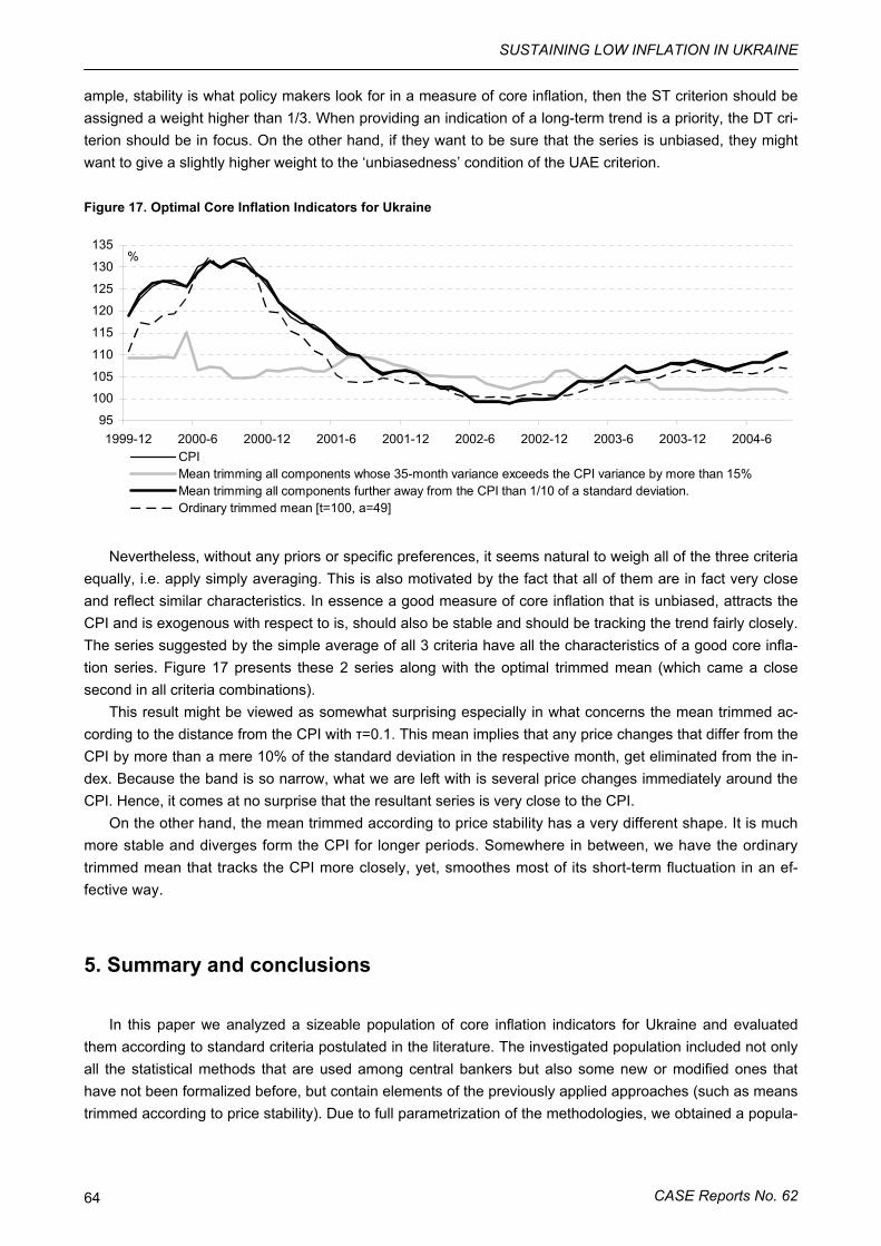
SUSTAINING LOW INFLATION IN UKRAINE
CASE Reports No. 62 64
ample, stability is what policy makers look for in a measure of core inflation, then the ST criterion should be assigned a weight higher than 1/3. When providing an indication of a long-term trend is a priority, the DT cri-terion should be in focus. On the other hand, if they want to be sure that the series is unbiased, they might want to give a slightly higher weight to the ‘unbiasedness’ condition of the UAE criterion.
Figure 17. Optimal Core Inflation Indicators for Ukraine
95
100
105
110
115
120
125
130
135
1999-12 2000-6 2000-12 2001-6 2001-12 2002-6 2002-12 2003-6 2003-12 2004-6CPIMean trimming all components whose 35-month variance exceeds the CPI variance by more than 15% Mean trimming all components further away from the CPI than 1/10 of a standard deviation.Ordinary trimmed mean [t=100, a=49]
%
Nevertheless, without any priors or specific preferences, it seems natural to weigh all of the three criteria equally, i.e. apply simply averaging. This is also motivated by the fact that all of them are in fact very close and reflect similar characteristics. In essence a good measure of core inflation that is unbiased, attracts the CPI and is exogenous with respect to is, should also be stable and should be tracking the trend fairly closely. The series suggested by the simple average of all 3 criteria have all the characteristics of a good core infla-tion series. Figure 17 presents these 2 series along with the optimal trimmed mean (which came a close second in all criteria combinations).
This result might be viewed as somewhat surprising especially in what concerns the mean trimmed ac-cording to the distance from the CPI with τ=0.1. This mean implies that any price changes that differ from the CPI by more than a mere 10% of the standard deviation in the respective month, get eliminated from the in-dex. Because the band is so narrow, what we are left with is several price changes immediately around the CPI. Hence, it comes at no surprise that the resultant series is very close to the CPI.
On the other hand, the mean trimmed according to price stability has a very different shape. It is much more stable and diverges form the CPI for longer periods. Somewhere in between, we have the ordinary trimmed mean that tracks the CPI more closely, yet, smoothes most of its short-term fluctuation in an ef-fective way.
5. Summary and conclusions
In this paper we analyzed a sizeable population of core inflation indicators for Ukraine and evaluated them according to standard criteria postulated in the literature. The investigated population included not only all the statistical methods that are used among central bankers but also some new or modified ones that have not been formalized before, but contain elements of the previously applied approaches (such as means trimmed according to price stability). Due to full parametrization of the methodologies, we obtained a popula-
Hryvniv V., Jakubiak M., Mykhaylychenko M., Novoseletska O., Paczynski W., Wozniak P.
CASE Reports No. 63 65
tion of 15706 series that can be considered comprehensive and complete when it comes to statistically cal-culated core series.
The population of core inflation series was evaluated using a set of 3 criteria each of which refers to the desirable properties of a core inflation indicator. Altogether, these criteria ensure that the indicator that will score high in the ranking will • Be unbiased; • Have the attraction property, i.e. it will “pull in” the CPI whenever it drifts away from the core inflation in-
dicator; • Be exogenous with respect to the CPI; • Track the trend inflation well; • Be stable in terms of both levels and first differences.
The final choices made using these criteria are visible in figure 17. The 3 core series are relatively different and hence a problem of recommending a single indicator comes up. It seems that the mean trimmed according to the distance from the center of the distribution is not a very good candidate since it differs only marginally from the CPI and does not offer a particularly good insight into the future developments of the CPI. Not surpris-ingly, this series scores very low on the stability criterion (see figures 15 and 16).
On the other hand, the mean trimmed according to price stability might be too far away from the actual CPI, to be accepted as a good core inflation indicator. The mean suggests a falling inflation trend during last couple of months while many other credible indicators of inflation processes in Ukraine suggest otherwise.
Undoubtedly the best candidate is the ordinary trimmed mean with parameters very close to the median (or the 47th percentile). It is relatively smooth and seems to have coped very well with reducing short-term volatility and staying relatively close to the CPI.
It has to be mentioned that while ordinary trimmed means are used by many central banks (e.g. Bank of England, National Bank of Poland), the other types of trimmed means, and particularly, the means trimmed according to deviation from the CPI, have not been used officially, to the best of our knowledge, in any cen-tral bank. Thus, if the National Bank of Ukraine decides to introduce core inflation to its official indicators, for practical reasons, it might be easier to start with ordinary trimmed means. Furthermore, all of the trimmed means used at central banks are symmetric means, even though some authors (Marques et al. 2000, Wozniak 2001) suggest that asymmetric trimmed means might be more efficient. For simplicity, we might suggest that the trimmed mean, instead of parameters (92,47), (88, 48) or (100,49) might be also calculated with the simpler parameters to produce a very similar result: asymmetry =50 and the total trim close to 100. The most intuitive choice is the median (100,50) or symmetric trimmed mean (90, 50). The former indicator has been calculated and actively used as a core inflation measure at the Bank of Canada and the National Bank of Poland.
Another core inflation indicator which is widely applied by central banks is exclusion-based mean. Its differ-ent modifications are used in USA, Poland, EU and others. Figure 14 presents best choice of this indicator for Ukraine. Although none of them fulfill UAE criterion, they are quite stable and track the inflation trend pretty good (Figures 15, 16). Their visual analysis evidence that they might be useful for the NBU as well.
Summing up we have to conclude, that the somewhat surprising, or even disappointing, results might be due to several factors. The most important, in our opinion is the dataset used for our analysis. As was men-tioned in section 3.1, our dataset contains 85 individual components, of which the last is a residual category introduced to ensure that the weighted average of the dataset equals the CPI. Visual inspection of this compo-nent indicates that it is one of the most volatile components of the entire basket. Thus, it gets eliminated very often in the processes of applying all the component-blind methods (i.e. all methods except for the exclusion-based method), leaving the basket without the important “stabilizing” element. This might be one of the reasons why the resulting core inflation series seem rather chaotic, volatile or far away from the actual CPI.
Another possible reason is that the length of the analyzed sample is far too short for cointegration analy-sis to be credible. Since the UAE criterion checks for unbiasedness and the presence of the error correction
SUSTAINING LOW INFLATION IN UKRAINE
CASE Reports No. 62 66
mechanism, it refers to long-term processes. However, our analysis is based on a mere 58 observations, far too few to justify using such an approach.
Therefore, research on this important issue needs to be continued and refined. Nonetheless, our current results, which we view as a first research-based recommendation in the area of alternative inflation measures in Ukraine, deserve closer attention of the NBU. We think that the core inflation series indicated by the analysis, constitute a very good alternative to conventional inflation measures, and is implemented by the NBU, they will undoubtedly improve understanding of inflationary processes in Ukraine and facilitate their control.
References
Bryan and Cecchetti (1996) Inflation and the Distribution of Price Changes, NBER Working Paper No. 5793.
Cecchetti, Stephen G. (1996) Measuring Short-Run Inflation for Central Bankers, NBER Working Paper No. 5786.
Eckstein, Otto (1981) Core Inflation, Prentice Hall. Freeman, D.G. (1998) Do Core Inflation Measures Help Forecast Inflation?, Economic Letters, 58, 143-147. Kearns Jonathan, (1998) The distribution and Measurement of Inflation, Reserve Bank of Australia Dis-
cussion Paper No. 9810, RBA1998. Marques, C. R. i João Machado Mota (2000) Using the Asymmetric Trimmed Mean as a Core Inflation
Indicator, Banco de Portugal Working Paper WP 6-00, Banco de Portugal. Marques, C.R., P. D. Neves i A. Goncalves da Silva (2000) Why should Central Banks avoid the use od
the underlying inflation indicator?, Banco de Portugal Working Paper WP 5-00, Banco de Portugal. Marques, C.R., P.D. Neves i L.M. Sarmento (2000) Evaluating Core Inflation Indicators, Banco de Portu-
gal Working Paper WP 3-00, Banco de Portugal. Meyler, Aidan (1999) A Statistical Measure of Core Inflation, Central Bank of Ireland Technical Paper
2/RT/99, Central Bank of Ireland. Petrik and Polovnyov (2002) Базова інфляція: концепція та деякі методи розрахунку (Core inflation:
concept and some methods of calculation), Visnyk NBY, December 2002, pp.47-48. Petrik and Polovnyov (2003) Проблема вибору цільового показника монетарної політики
Національного банку України (Problem of choosing of target indicator for monetary policy of the National Bank of Ukraine), Visnyk NBY, July 2003, 8-14.
Quah, D. and S. P. Vahey (1995) Measuring Core Inflation. The Economic Journal No.105, 1130-1144. Roger, Scott (1995) Measures of Underlying Inflation in New Zealand, 1981-1995, Reserve Bank of New
Zealand Discussion Paper G95/5. Roger, Scott (1994) Alternative Measures of Underlying Inflation in New Zealand, Reserve Bank of New
Zealand Bulletin Vol. 57(2) 109-129. Roger, Scott (1997) A Robust Measure of Underlying Inflation in New Zealand, 1949-1996, Reserve
Bank of New Zealand Discussion Paper G97/7. Wozniak Przemyslaw (2002) Inflacja bazowa (Core inflation), a book in the CASE-Library series, Center
for Social and Economic Research, Warsaw. Wozniak, Przemyslaw (2001) Perspectives of using trimmed means for analyzing core inflation in Poland
(Możliwości wykorzystania średnich obciętych do analizy inflacji bazowej w Polsce), Materiały i Studia no. 117 (NBP Working Paper Series no. 117), National Bank of Poland, www.nbp.pl.

Hryvniv V., Jakubiak M., Mykhaylychenko M., Novoseletska O., Paczynski W., Wozniak P.
CASE Reports No. 63 67
Chapter 5: Monetary Transmission Research in Europe: Lessons for Ukraine
Wojciech Paczynski*
1. Introduction
The term ‘transmission mechanism of the monetary policy’ is applied to the whole process in which cen-tral bank’s monetary policy actions affect macroeconomic variables such as economic activity and price de-velopments. Given the perceived rising importance of monetary policy in promoting sustainable growth and stability of economies (Mishkin, 1996) the recent years saw an intensification of efforts to understand, de-scribe and draw policy relevant lessons from the nature of monetary transmission processes.
This effort has clearly resulted in better understanding of the broad features of the monetary transmis-sion, though it should be stressed that complexity of the process, differences between countries and instabil-ity of the relationships over time all result in there being no unique and undisputed view of all the aspects involved (ECB, 2004).
This paper aims at providing an overview of recent monetary transmission research in Europe that is then used to pose some open questions concerning the future of related work on Ukrainian economy. Sec-tion two sketches the analytical framework that is most commonly used in the analysis of monetary transmis-sion process. Next section discusses some institutional features that affect the nature of the transmission process itself and analytical approaches to it. A quick guide to empirical strategies and typical results they produce in other countries can be found in section four. Concluding section offers a view on the research agenda for Ukraine that draws from the experience of work on other European economies and from specific features of the Ukrainian economy.
2. Steps and channels of monetary transmission
Since the interactions between monetary policy decisions and the behaviour of various macroeco-nomic variables are very complex, it is useful to organise the discussion by introducing some classifica-tions and structure. For simplicity of the exposition we assume here that a major tool of the monetary pol-icy is setting the official interest rates (which is true in countries with floating exchange rates; in an envi-ronment of the fixed exchange rate regime monetary authorities’ ability to impact interest rates is limited; rates are normally determined by the developments in an economy using a currency that serves as an an-chor of the peg). One important classification (cf. Bank of England, 1999) distinguishes two steps in which the monetary policy operates: * I am thankful to Małgorzata Jakubiak and Przemysław Woźniak for comments. The usual disclaimer applies.
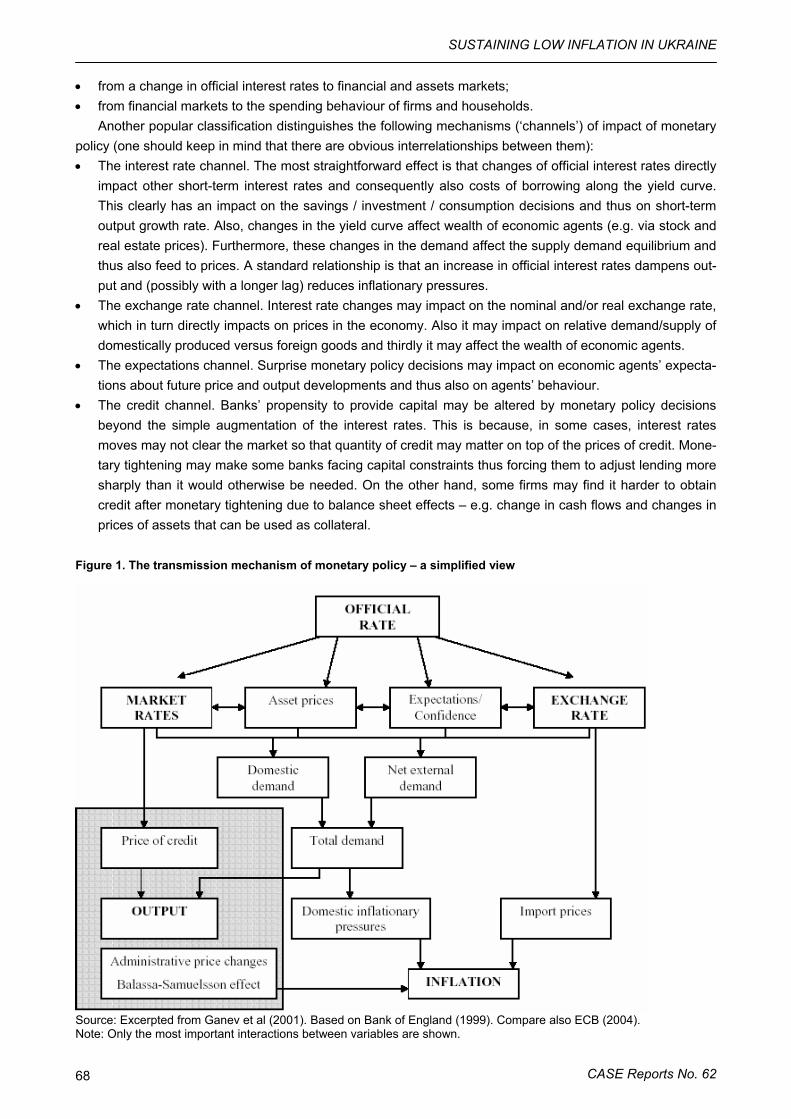
SUSTAINING LOW INFLATION IN UKRAINE
CASE Reports No. 62 68
• from a change in official interest rates to financial and assets markets; • from financial markets to the spending behaviour of firms and households.
Another popular classification distinguishes the following mechanisms (‘channels’) of impact of monetary policy (one should keep in mind that there are obvious interrelationships between them): • The interest rate channel. The most straightforward effect is that changes of official interest rates directly
impact other short-term interest rates and consequently also costs of borrowing along the yield curve. This clearly has an impact on the savings / investment / consumption decisions and thus on short-term output growth rate. Also, changes in the yield curve affect wealth of economic agents (e.g. via stock and real estate prices). Furthermore, these changes in the demand affect the supply demand equilibrium and thus also feed to prices. A standard relationship is that an increase in official interest rates dampens out-put and (possibly with a longer lag) reduces inflationary pressures.
• The exchange rate channel. Interest rate changes may impact on the nominal and/or real exchange rate, which in turn directly impacts on prices in the economy. Also it may impact on relative demand/supply of domestically produced versus foreign goods and thirdly it may affect the wealth of economic agents.
• The expectations channel. Surprise monetary policy decisions may impact on economic agents’ expecta-tions about future price and output developments and thus also on agents’ behaviour.
• The credit channel. Banks’ propensity to provide capital may be altered by monetary policy decisions beyond the simple augmentation of the interest rates. This is because, in some cases, interest rates moves may not clear the market so that quantity of credit may matter on top of the prices of credit. Mone-tary tightening may make some banks facing capital constraints thus forcing them to adjust lending more sharply than it would otherwise be needed. On the other hand, some firms may find it harder to obtain credit after monetary tightening due to balance sheet effects – e.g. change in cash flows and changes in prices of assets that can be used as collateral.
Figure 1. The transmission mechanism of monetary policy – a simplified view
Source: Excerpted from Ganev et al (2001). Based on Bank of England (1999). Compare also ECB (2004). Note: Only the most important interactions between variables are shown.
Hryvniv V., Jakubiak M., Mykhaylychenko M., Novoseletska O., Paczynski W., Wozniak P.
CASE Reports No. 63 69
While such classifications (the one given above is not unique – e.g. ‘expectation channel’ is not always treated separately, some authors also distinguish the ‘asset prices channel’ with regard to assets ranging from currencies to bonds, real estate, stocks, etc.) are useful in organising the discussion, it is often difficult to clearly distinguish between channels and it is usually even more difficult to asses relative importance of channels.
The traditional treatment of the interest rate channel usually abstracts from the effects of interest rate changes on agents’ expectations and also on the price on currencies and other assets. The underlying the-ory is based on the assumptions that central banks have some influence on the real interest rates and not only nominal rates and secondly, that components of aggregate demand are interest sensitive (Juks, 2004).
While the manipulation of monetary policy instruments (such as official interest rates) clearly is the major tool of conducting monetary policy and most empirical studies concentrate on the analysis of their impact, there are also other less formalised methods of exerting impact on financial markets and consequently pos-sibly also on investment and consumption decisions. The most important of these is probably control of and manipulation of information, e.g. issuing news to market participants that impact on their expectations of fu-ture policy actions. Examples of such news include any central bankers’ comments on the expected/intended ERM II accession dates in non-euro EU member states, comments on the possibility of corrections to the whole monetary policy regime, comments on the exchange rate trends (in countries where central banks oc-casionally intervene in the forex market), comments on inflation forecasts (in countries where central banks are focused on price developments).
3. Monetary policy regimes, institutional arrangements and the scope for monetary policy
Clearly, the nature of the transmission mechanism is crucially affected by the monetary policy regime (Mayes, 2004b). In the world of liberalised capital account central banks can control the price of money (in-terest rates) or the quantities of money provided or, alternatively, the exchange rate of the domestic cur-rency, or some combinations thereof. In a (credible) fixed exchange rate regime with full convertibility of the currency the central bank effectively looses the control on interest rates and money creation. Since domestic and anchor currencies are fully exchangeable, domestic interest rates should follow the rates in the anchor currency with some (possibly time varying) risk premium. However, one should keep in mind that even in a floating exchange rate system, the ability of small open economies to set interest rates fully independently is limited by the impact of external factors (Dąbrowski, 2002) and it is not a coincidence that we typically ob-serve co-movements in interest rates in world economies. Indeed, as noted by Mayes (2004a): ‘Inside or outside a monetary union small countries simply have to accept the monetary decisions that relate to the needs of the larger countries and work out a strategy for adapting to them with a minimum of real cost to their citizens. The scope for running a divergent monetary policy despite different domestic shocks and re-quirements is small.’ An interesting piece of empirical evidence supporting this view is provided by Frankel et al. (2002). They study the behaviour of interest rates in the large sample of developing and industrialised economies during the last three decades. The conclusion is that in the long run there is almost full transmis-sion of international interest rates to local rates, perhaps with the exception of the largest industrialised economies (US, Japan, Germany) who are thus the only ones able to possibly adopt independent monetary policy. In the short run, exchange rate regimes appear to matter with the intuitive result that countries adopt-ing more flexible regimes have more room of manoeuvre for (temporary) independent monetary policy since local rates adjust slower to movements in international rates. This finding is corroborated by Shambaugh (2004). The situation would look different for countries with efficient capital controls. Still, in the long run effi-ciency of capital control can be debatable.
SUSTAINING LOW INFLATION IN UKRAINE
CASE Reports No. 62 70
The structure of the banking system and institutional arrangements surrounding it are another important elements impacting heavily on the nature of the monetary transmission process. This remains true also for highly developed economies with well developed banking and financial sectors such as EMU countries. In their study on the euro-zone, Ehrmann et al. (2003) list four aspects that could matter for monetary transmis-sion process: the importance of state influences in determining credit flows, the prevalence of relationship lending, the size of deposit insurance guarantees, and the extent of bank networks. It is no surprise that such issues matter even more in countries with less developed financial architecture, where the importance of the ‘credit channel’ of transmission is usually stronger. Also, institutional arrangements turn out important in in-fluencing the first stage of monetary transmission, i.e. from official interest rates to money market rates. In the context of the euro-zone Moschitz (2004) observes that ‘the behaviour of the overnight rate depends on reserve supply, but equally important on the institutional framework for the reserve market’.
Clearly, there are other institutional and other structural characteristics of countries that can potentially crucially affect the strength and speed of transmission of monetary policy to various economic indicators of interest to policy makers. Among the usual suspects one can mention the role of capital markets as proxied e.g. by stock market capitalisation, credibility of central bank policies, and the characteristics of the labour market (nature of wage contracts, etc.). Nevertheless, it is very difficult to formulate generally binding rules as to which combinations of country characteristics affect the transmission in which way, when. For obvious reasons, the scope of heterogeneity in such matters and their impact on divergences in the transmission of monetary policy were studied at length in the run-up to the introduction of the euro (e.g. Dornbusch et al. (1998), Mihov (2001)). Recently, Jarociński (2004) compared the nature of the transmission between Central and Eastern Europe on the one side and Western Europe on the other side to find some differences and some striking similarities in responses to monetary shocks. The results of Jarociński (2004) appear to em-pirically support the view that smaller financial sector on CEE countries, as compared to the euro-zone makes the economies in the first region less responsive to the monetary policy in the short-run. However, in medium- to long-term horizons, monetary policy in CEE appears to be quite effective. On a more general level, these findings illustrate the complicated nature of the links between institutional characteristics of coun-tries and the nature of monetary policy transmission.
4. Empirical approaches to monetary transmission
There is a multiplicity of empirical approaches to monetary transmission. One could classify them into the following broad categories: • less formalised studies using narrative, graphical and comparative arguments to make inference about
the factors at play and their relative importance, • studies using vector autoregressive (VAR) framework with relatively low data requirements and imposing
relatively mild theoretical assumptions, • studies based on small-scale structural macroeconomic models, • studies based on large-scale structural macroeconomic models, • studies based on microeconomic evidence on the behaviour of non-financial enterprises, • studies based on microeconomic evidence on banks’ behaviour.
4.1. Brief review of empirical literature Rather unsurprisingly, there is a vast literature looking at the effects of the monetary policy in the US.
These analyses benefit from the availability of long time series. Also, many advances in theoretical models behind monetary transmission analyses as well as empirical approaches were pioneered by researchers
Hryvniv V., Jakubiak M., Mykhaylychenko M., Novoseletska O., Paczynski W., Wozniak P.
CASE Reports No. 63 71
based in US universities. Classical references to articles reviewing the large body of monetary transmission research on the US include Leeper, Sims and Zha (1998) and Christiano, Eichenbaum and Evans (2000). Some recent advances in empirical approaches are presented in Uhlig (2001) and Bernanke et al. (2004).
The emergence of the European Central Bank and the introduction of the euro have boosted demand for better understanding of monetary transmission mechanism in the EU12. In 1999, Monetary Transmission Network was created involving ECB and euro-area central banks’ economists to comprehensively study the transmission of the monetary policy in the euro-area35. The outcome of this work was published in the ECB working paper series (no. 91-114) and subsequently in Angeloni, Kashyap and Mojon (2003). A summary of results can also be found in Angeloni et al. (2003). Elbourne and de Haan (2004) is an example of recent work from outside the ECB.
Ganev et al (2001) contain a fairly extensive survey of papers dealing with monetary transmission in Central and Easter Europe. Some more recent results and references to other interesting work can be found in Garbuza (2003), Schmitz (2004), Jarociński (2004) and EFN (2004). A review of the work on three Baltic States can be found in Bank of Estonia (2004).
4.2. Results for Poland This section reviews some of the results on monetary transmission in Poland and discusses the issues
involved in various approaches. It is intended to give an overview of results from various strands of literature in a country where data availability is an issue. It is worth bearing in mind that throughout the analysed pe-riod Polish monetary policy regime was gradually moving towards increased exchange rate flexibility with direct inflation targeting introduced in 1999. Recent years also saw a no-interventions policy of the central bank that did not try to affect the exchange rate of the zloty by entering the forex market.
Kokoszczyński et al. (2002) review results pertaining to monetary policy transmission in the Polish econ-omy using the variety of approaches. One set of results (see also Łyziak, 2002) is based on the small struc-tural model motivated by the framework of Clarida, Gali and Gertler (1999). Impulse response analysis re-veals a rather typical pattern. Output gap falls with a strongest impact felt 3 quarters after the initial monetary policy tightening. The strongest impact on inflation materialises after some 7-9 quarters.
While these results appear realistic and in line with some evidence pertaining to other countries they should be treated as providing just a rough approximation of monetary transmission in Poland in the period up to 2001 (1994-2001 data were used to estimate the underlying model). Kokoszczyński et al. (2002) note significant changes in impulse responses to monetary policy shocks depending on the version of the model employed and data sample used to estimate the model equations. This should not be surprising given the substantial changes in the whole monetary policy framework in Poland during the last 15 years (from various forms of pegged exchange rate regime to a free float), anyway short time series used to estimate models (implying large error margins) and simplicity of the model.
Another set of results comes from analysis based on identified vector autoregressions (VARs). Such an approach requires a selection of variables included in the analysis and a selection of identification schemes (to be able to simulate orthogonal shocks in one variable – interest rate). Kokoszczyński et al. (2002) and Wróbel and Pawłowska (2002) report the results for a three and five variables VARs with identification based on Choleski decomposition motivated by the sequencing of information available to market participants and a set of a-priori assumptions on which variables can impact the other when. Given the very short sample pe-riod for this analysis it is not surprising that some of the results appear to be consistent with the ‘consensus view’ on monetary transmission (e.g. Leeper, Sims and Zha (1998) and Christiano, Eichenbaum and Evans (2000)) while the other appear to contradict the common wisdom. Some surprises in the results of VAR analyses are not typical for Poland only. For instance there is a substantial variation in the results for individ-ual euro area countries as reported by Peersman and Smets (2001).
35 For more information on Monetary Transmission Network see http://www.ecb.int/home/html/researcher_mtn.en.html.
SUSTAINING LOW INFLATION IN UKRAINE
CASE Reports No. 62 72
Kokoszczyński et al. (2002) as well as Wróbel and Pawłowska (2002) also report some results concerning the first step of monetary policy transmission as defined in this paper, i.e. the reaction of commercial banks’ interest rates in response to central bank’s rates changes. The analysis based on error correction model (ECM) using aggregate data reveal that nearly all deposit rates adjust to official rates within around 3-4 months and credit rates appear to adjust very quickly (up to 4 months – visibly faster than in the euro area). Short and quite specific sample that covered mostly a period of interest rate declines did not allow for making any more robust inference about asymmetry of reactions, i.e. different patterns of banks’ responses to tightening and loosening monetary policy. The analysis based on panel data on individual banks reveals that credit adjustment is stronger in the case of small banks with low capital. It also produces a result of stronger adjustment in credit provision among more liquid banks (which is the opposite of what one usually finds in studies e.g. for the euro area). One should, however, be aware that the whole banking system was over-liquid throughout the period under investigation and that most of the period was characterised by monetary easing.
4.3. Selected results from other countries This section provides an overview of empirical work in some other economies that appear to be poten-
tially relevant for the future work on Ukraine. This selection is not based on any strictly defined rules and is certainly not extensive.
Results on monetary transmission in the Baltic States could be interesting from the Ukrainian perspec-tive. The major difference with the Polish case is that three Baltic States are much smaller and more open to trade economies and that they have followed the fixed exchange rate regime for the last few years in an en-vironment of liberalised capital account. An implication of this is that there has been very limited scope for discretionary monetary policy on the side of central banks. In practice their actions can be confined to con-trolling the reserve/liquidity requirements and possibly playing the role of the lender-of-last-resort. For exam-ple Vetlov (2004) describes the experience of the Bank of Lithuania that in an environment of the currency board regime was experimenting with carrying out open market operations in the 1997-1999 period. These actions were firstly motivated by plans to gradually abandon the currency board arrangements. However, after the decision was made that in view of external shocks (Asian and Russian crises) the original exchange rate arrangement should be maintained, the Bank soon realised that there was little need for open market operations, little guidance as to what the optimal interest rate strategy should be and that continuing with conducting such operations could send unwanted signals to market participants. Consequently, open market operations were abandoned.
Bank of Estonia (2004) reviews the results for the three Baltic States generated using small scale struc-tural models developed at the respective central banks. One difficulty in modelling is how to incorporate monetary policy shocks in a way that would be consistent with the overall monetary system (e.g. interest rates are not under the control of central bank). The results are generally in line with those obtained for European advanced economies and specific features of reaction functions appear to be very much model dependant, thus their detailed description is skipped here.
EFN (2004) provide a set of results from VAR analyses using relatively recent data for a number of EU new member states. The identification scheme is by Choleski decomposition using different orderings of variables for countries with relatively independent monetary policy (Czech Republic, Poland, Hungary, Slovak Republic and Slovenia) and for countries with fixed exchange rate regimes (Estonia, Latvia and Lithuania). The results for the majority of countries are broadly similar to the results found for the euro-zone, though the error bands of impulse responses are wide such that differences in observed average impulse responses are unlikely to be significant. This illustrates the problems with the VAR analysis using simple identification schemes in countries with data limitations. In the Czech Republic, output contracts strongly in response to monetary tightening, while prices appear to actually be rising for at least 1.5 years after monetary tightening (price puzzle). In Hungary, the reaction of both output and prices is of expected sign (though not statistically significant), very prompt (maxi-
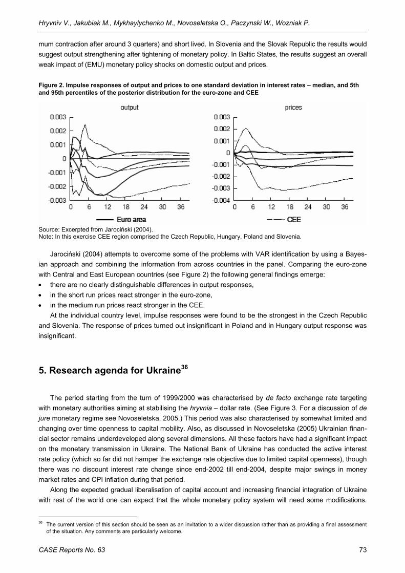
Hryvniv V., Jakubiak M., Mykhaylychenko M., Novoseletska O., Paczynski W., Wozniak P.
CASE Reports No. 63 73
mum contraction after around 3 quarters) and short lived. In Slovenia and the Slovak Republic the results would suggest output strengthening after tightening of monetary policy. In Baltic States, the results suggest an overall weak impact of (EMU) monetary policy shocks on domestic output and prices.
Figure 2. Impulse responses of output and prices to one standard deviation in interest rates – median, and 5th and 95th percentiles of the posterior distribution for the euro-zone and CEE
Source: Excerpted from Jarociński (2004). Note: In this exercise CEE region comprised the Czech Republic, Hungary, Poland and Slovenia.
Jarociński (2004) attempts to overcome some of the problems with VAR identification by using a Bayes-ian approach and combining the information from across countries in the panel. Comparing the euro-zone with Central and East European countries (see Figure 2) the following general findings emerge: • there are no clearly distinguishable differences in output responses, • in the short run prices react stronger in the euro-zone, • in the medium run prices react stronger in the CEE.
At the individual country level, impulse responses were found to be the strongest in the Czech Republic and Slovenia. The response of prices turned out insignificant in Poland and in Hungary output response was insignificant.
5. Research agenda for Ukraine36
The period starting from the turn of 1999/2000 was characterised by de facto exchange rate targeting with monetary authorities aiming at stabilising the hryvnia – dollar rate. (See Figure 3. For a discussion of de jure monetary regime see Novoseletska, 2005.) This period was also characterised by somewhat limited and changing over time openness to capital mobility. Also, as discussed in Novoseletska (2005) Ukrainian finan-cial sector remains underdeveloped along several dimensions. All these factors have had a significant impact on the monetary transmission in Ukraine. The National Bank of Ukraine has conducted the active interest rate policy (which so far did not hamper the exchange rate objective due to limited capital openness), though there was no discount interest rate change since end-2002 till end-2004, despite major swings in money market rates and CPI inflation during that period.
Along the expected gradual liberalisation of capital account and increasing financial integration of Ukraine with rest of the world one can expect that the whole monetary policy system will need some modifications.
36 The current version of this section should be seen as an invitation to a wider discussion rather than as providing a final assessment
of the situation. Any comments are particularly welcome.
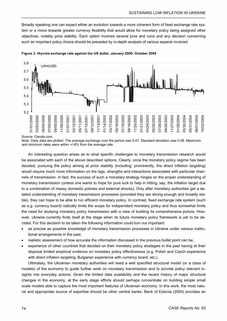
SUSTAINING LOW INFLATION IN UKRAINE
CASE Reports No. 62 74
Broadly speaking one can expect either an evolution towards a more coherent form of fixed exchange rate sys-tem or a move towards greater currency flexibility that would allow for monetary policy being assigned other objectives, notably price stability. Each option involves several pros and cons and any decision concerning such an important policy choice should be preceded by in-depth analysis of various aspects involved.
Figure 3. Hryvnia exchange rate against the US dollar, January 2000- October 2004
5.2
5.3
5.4
5.5
5.6
5.7
5.8
01/0
1/20
00
03/0
3/20
00
05/0
4/20
00
07/0
5/20
00
09/0
5/20
00
11/0
6/20
00
01/0
7/20
01
03/1
0/20
01
05/1
1/20
01
07/1
2/20
01
09/1
2/20
01
11/1
3/20
01
01/1
4/20
02
03/1
7/20
02
05/1
8/20
02
07/1
9/20
02
09/1
9/20
02
11/2
0/20
02
01/2
1/20
03
03/2
4/20
03
05/2
5/20
03
07/2
6/20
03
09/2
6/20
03
11/2
7/20
03
01/2
8/20
04
03/3
0/20
04
05/3
1/20
04
08/0
1/20
04
10/0
2/20
04
UAH/USD
Source: Oanda.com. Note: Daily data are plotted. The average exchange over the period was 5.47. Standard deviation was 0.08. Maximum and minimum rates were within +/-6% from the average rate.
An interesting question arises as to what specific challenges to monetary transmission research would be associated with each of the above described options. Clearly, once the monetary policy regime has been decided, pursuing the policy aiming at price stability (including, prominently, the direct inflation targeting) would require much more information on the lags, strengths and interactions associated with particular chan-nels of transmission. In fact, the success of such a monetary strategy hinges on the proper understanding of monetary transmission (unless one wants to hope for pure luck to help in hitting, say, the inflation target due to a combination of messy domestic policies and external shocks). Only after monetary authorities get a de-tailed understanding of monetary transmission processes (provided they are strong enough and broadly sta-ble), they can hope to be able to run efficient monetary policy. In contrast, fixed exchange rate system (such as e.g. currency board) radically limits the scope for independent monetary policy and thus somewhat limits the need for studying monetary policy transmission with a view of building its comprehensive picture. How-ever, Ukraine currently finds itself at the stage when its future monetary policy framework is yet to be de-cided. For this decision to be taken the following information could turn out important: • as precise as possible knowledge of monetary transmission processes in Ukraine under various institu-
tional arrangements in the past, • realistic assessment of how accurate the information discussed in the previous bullet point can be, • experience of other countries that decided on their monetary policy strategies in the past having at their
disposal limited empirical evidence on monetary policy effectiveness (e.g. Polish and Czech experience with direct inflation targeting, Bulgarian experience with currency board, etc.). Ultimately, the Ukrainian monetary authorities will need a well specified structural model (or a class of
models) of the economy to guide further work on monetary transmission and to provide policy relevant in-sights into everyday actions. Given the limited data availability and the recent history of major structural changes in the economy, at the early stage efforts should perhaps concentrate on building simple small scale models able to capture the most important features of Ukrainian economy. In this work, the most natu-ral and appropriate source of expertise should be other central banks. Bank of Estonia (2004) provides an
Hryvniv V., Jakubiak M., Mykhaylychenko M., Novoseletska O., Paczynski W., Wozniak P.
CASE Reports No. 63 75
interesting overview and discussion of the models developed in the three Baltic States. This experience of alternative modelling approaches and ensuing differences in model behaviour might be worth looking at given the otherwise similar characteristics of the countries. Another potentially interesting lessons can be drawn from the analysis of small scale models such as Bank of Finland’s EDGE model for the euro area (Kortelainen, 2002), FPS model for the New Zealand (Black et al., 1997), small structural model of the Na-tional Bank of Poland (Łyziak, 2002), some of the (very well documented) models used at the Bank of Eng-land (Bank of England, 2000) and several other.
Clearly, the historical record provides a far-from-perfect data source for elaboration of empirical specifi-cations. As noted by van Aarle et al. (2004) ‘the monetary transmissions are still subject to uncertainties as witness e.g. volatile velocity and money multipliers, making econometric testing difficult’. Thus, in learning about monetary transmission mechanism it appears that the best approach is of extracting all possible infor-mation from existing data on Ukraine and at the same time closely monitoring the results obtained for other countries that share some important characteristics with Ukraine. Institutional aspects surrounding the finan-cial sector as a whole and de facto monetary policy framework are important elements that should not be overlooked in the analysis.
References
Angeloni, Ignazio, Anil Kashyap and Benoît Mojon (2003) Monetary Policy Transmission in the Euro Area. A Study by the Eurosystem Monetary Transmission Network, Cambridge University Press.
Angeloni, Ignazio, Anil Kashyap, Benoît Mojon and Daniele Terlizzese (2003) Monetary Policy Transmis-sion in the Euro: Does the Interest Rate Channel Explain All? NBER Working Paper 9984.
Bank of England (1999) The transmission mechanism of monetary policy, report prepared under the guidance of the Monetary Policy Committee, www.bankofengland.co.uk.
Bank of England (2000) Economic Models at the Bank of England: September 2000 Update, www.bankofengland.co.uk.
Bank of Estonia (2004) The Monetary Transmission Mechanism in the Baltic States, Tallin. Bernanke, Ben S., Jean Boivin and Piotr Elisasz (2004) Measuring the Effects of Monetary Policy: A Fac-
tor-Augmented Vector Autoregressive (FAVAR) Approach, NBER Working Paper 10220. Black, R., Cassino, V., Drew, A., Hansen, E., Hunt, B., Rose, D. and Scott, A. (1997) The Forecasting
and Policy System: the Core Model, Reserve Bank of New Zealand Research Paper, No. 43, August. Christiano Lawrence J., Martin Eichenbaum, Charles L. Evans (2000) Monetary policy shocks: What have
we learned and to what end? J. Taylor and M. Woodford (eds.), Handbook of Macroeconomics, North Holland. Clarida, Richard, Jordi Gali, and Mark Gertler (1999) The Science of Monetary Policy: A New Keynesian
Perspective, Journal of Economic Literature, 37, pp. 1661–1707. Dąbrowski, Marek (2002) Is there a room for national monetary policy in the era of globalization? paper
presented at the GDN Fourth Annual Conference, http://www.gdnet.org/pdf/2002AwardsMedalsWinners/FinancialMarkets/marek_dabrowski_paper.pdf.
Dornbusch, Rudiger, Carlo A. Favero and Francesco Giavazzi (1998) Immediate Challenges for the European Central Bank, Economic Policy, 26, 15-64.
ECB (2004) The Monetary Policy of the ECB, European Central Bank, Frankfurt am Main. EFN (2004) Monetary Transmission in Acceding Countries, Annex 4 of the European Forecasting Net-
work Spring 2004 Report, http://www.efn.uni-bocconi.it/. Ehrmann Michael., L. Gambacorta, J. Martínez-Pagés, P. Sevestre and A. Worms (2003) Financial sys-
tems and the role of banks in monetary policy transmission in the euro area, Chapter 14, in I. Angeloni, A. Kashyap and B. Mojon (eds.) Monetary Transmission in the Euro Area, Cambridge University Press.
SUSTAINING LOW INFLATION IN UKRAINE
CASE Reports No. 62 76
Frankel, Jeffrey A., Sergio L. Schmukler and Luis Serven (2002) Global Transmission of Interest Rates: Monetary Independence and Currency Regime, NBER Working Paper 8828.
Gavev, Georgy, Krisztina Molnar, Krzysztof Rybinski and Przemyslaw Wozniak (2001) Transmission Mechanisms of Monetary Policy in Central and Eastern Europe, mimeo, CERGE-EI, http://www.cerge-ei.cz/pdf/gdn/RRCI_09_paper_01.pdf .
Garbuza, Yuriy (2003) The Transmission Mechanism of Monetary Policy: Investigating the Exchange Rate Channel for Central and East European Countries, National University of ‘Kyiv-Mohyla Academy’, MA thesis.
Jarociński, Marek (2004) Responses to Monetary Policy Shocks in the East and West of Europe: A Comparison, CASE Studies & Analyses No. 287.
Juks, Reimo (2004) Monetary Policy Transmission Mechanisms: a Theoretical and Empirical Overview, in Bank of Estonia, The Monetary Transmission Mechanism in the Baltic States, Tallin.
Kokoszczyński, Ryszard, Tomasz Łyziak, Małgorzata Pawłowska, Jan Przystupa and Ewa Wróbel (2002) Mechanizm transmisji polityki pieniężnej – współczesne ramy teoretyczne, nowe wyniki empiryczne dla Pol-ski (Monetary transmission mechanisms – theoretical basis and new empirical results for Poland), Materiały i Studia NBP nr 151.
Kortelainen, M. (2002) EDGE: A Model of the Euro Area with Applications to Monetary Policy, Helsinki: Bank of Finland Study, No. E23.
Leeper E, Sims C. and T. Zao (1998) What does monetary policy do? Brookings Papers on Economic Activity, 2, pp. 1-78.
Łyziak, Tomasz (2002) Monetary transmission mechanism in Poland. The strength and delays, Materiały i Studia NBP Paper 26.
Mayes, David G. (2004a) Introduction, in Bank of Estonia, The Monetary Transmission Mechanism in the Baltic States, Tallin.
Mayes, David G. (2004b) The Monetary Transmission Mechanism in the Baltic States, in Bank of Esto-nia, The Monetary Transmission Mechanism in the Baltic States, Tallin.
Mihov, I. (2001) Monetary Policy Implementation and Transmission in the European Monetary Union, Economic Policy, 33, 371-406.
Mishkin, Frederic S. (1996) The Channels of Monetary Transmission: Lessons for Monetary Policy, NBER Working Paper 5464.
Moschitz, Julius (2004) The Determinant of the Overnight Interest Rate in the Euro Area, ECB Working Paper No. 393.
Novoseletska, O. (2005) Ukrainian Money Market. In: Jakubiak (ed.) Sustaining Low Inflation in Ukraine. CASE Report No. 63.
Peersman, Gert and Frank Smets (2001) The Monetary Transmission Mechanism in the Euro Area: More Evidence from VAR Analysis, ECB Working Paper No. 91.
Shambaugh, Jay C. (2004) The Effect of Fixed Exchange Rates on Monetary Policy, Quarterly Journal of Economics, 119 (1), 301-351.
Schmitz, Birgit (2004) What Role do Banks Play in Monetary Policy Transmission in EU Accession Coun-tries, paper presented at the European University Institute conference in Florence, May.
Uhlig, Harald (2001) What are the Effects of Monetary Policy on Output? Results from an Agnostic Identi-fication Procedure, Center for Economic Research Discussion Paper 1999-28, Tilburg University.
Van Aarle, Bas, Eelke de Long and Robert Sosoian (2004) Macroeconomic Stabilization in Ukraine: Is it Sustainable? paper presented during Study Group on ‘Monetary Policy in Selected CIS Countries’ meeting, Bruges, July.
Vetlov, Igor (2004) The Monetary Transmission Mechanism in Lithuania, in Bank of Estonia, The Mone-tary Transmission Mechanism in the Baltic States, Tallin.
Wróbel, Ewa and Małgorzata Pawłowska (2002) Monetary transmission in Poland: some evidence on in-terest rate and credit channels, Materiały i Studia NBP Paper 24.
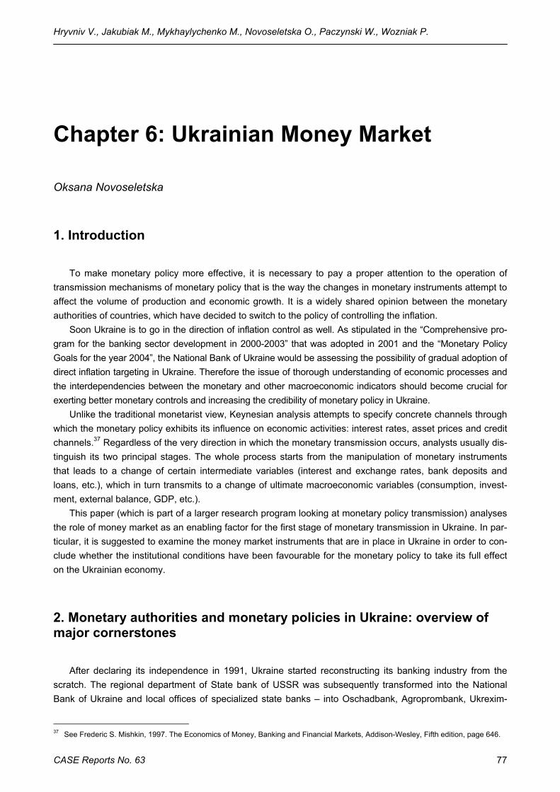
Hryvniv V., Jakubiak M., Mykhaylychenko M., Novoseletska O., Paczynski W., Wozniak P.
CASE Reports No. 63 77
Chapter 6: Ukrainian Money Market
Oksana Novoseletska
1. Introduction
To make monetary policy more effective, it is necessary to pay a proper attention to the operation of transmission mechanisms of monetary policy that is the way the changes in monetary instruments attempt to affect the volume of production and economic growth. It is a widely shared opinion between the monetary authorities of countries, which have decided to switch to the policy of controlling the inflation.
Soon Ukraine is to go in the direction of inflation control as well. As stipulated in the “Comprehensive pro-gram for the banking sector development in 2000-2003” that was adopted in 2001 and the “Monetary Policy Goals for the year 2004”, the National Bank of Ukraine would be assessing the possibility of gradual adoption of direct inflation targeting in Ukraine. Therefore the issue of thorough understanding of economic processes and the interdependencies between the monetary and other macroeconomic indicators should become crucial for exerting better monetary controls and increasing the credibility of monetary policy in Ukraine.
Unlike the traditional monetarist view, Keynesian analysis attempts to specify concrete channels through which the monetary policy exhibits its influence on economic activities: interest rates, asset prices and credit channels.37 Regardless of the very direction in which the monetary transmission occurs, analysts usually dis-tinguish its two principal stages. The whole process starts from the manipulation of monetary instruments that leads to a change of certain intermediate variables (interest and exchange rates, bank deposits and loans, etc.), which in turn transmits to a change of ultimate macroeconomic variables (consumption, invest-ment, external balance, GDP, etc.).
This paper (which is part of a larger research program looking at monetary policy transmission) analyses the role of money market as an enabling factor for the first stage of monetary transmission in Ukraine. In par-ticular, it is suggested to examine the money market instruments that are in place in Ukraine in order to con-clude whether the institutional conditions have been favourable for the monetary policy to take its full effect on the Ukrainian economy.
2. Monetary authorities and monetary policies in Ukraine: overview of major cornerstones
After declaring its independence in 1991, Ukraine started reconstructing its banking industry from the scratch. The regional department of State bank of USSR was subsequently transformed into the National Bank of Ukraine and local offices of specialized state banks – into Oschadbank, Agroprombank, Ukrexim-
37 See Frederic S. Mishkin, 1997. The Economics of Money, Banking and Financial Markets, Addison-Wesley, Fifth edition, page 646.
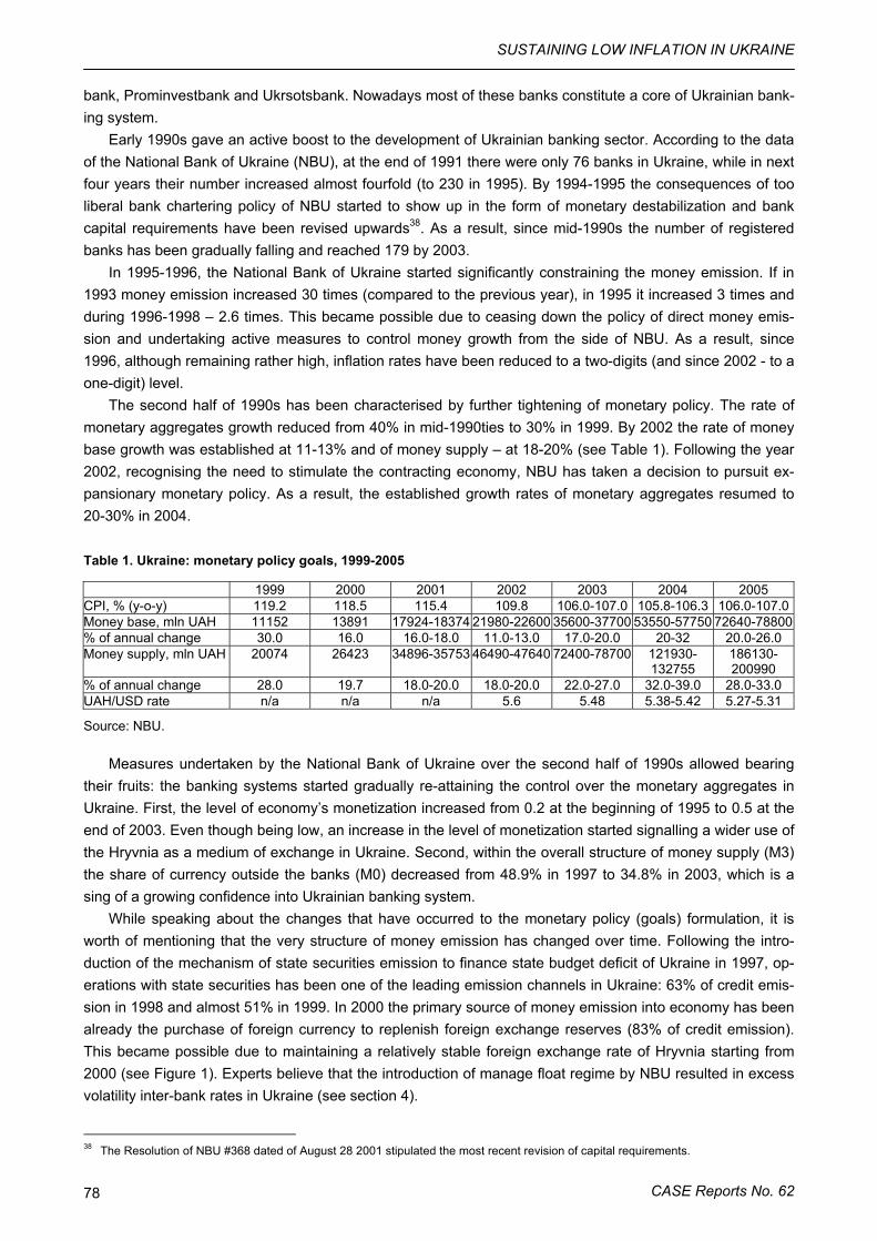
SUSTAINING LOW INFLATION IN UKRAINE
CASE Reports No. 62 78
bank, Prominvestbank and Ukrsotsbank. Nowadays most of these banks constitute a core of Ukrainian bank-ing system.
Early 1990s gave an active boost to the development of Ukrainian banking sector. According to the data of the National Bank of Ukraine (NBU), at the end of 1991 there were only 76 banks in Ukraine, while in next four years their number increased almost fourfold (to 230 in 1995). By 1994-1995 the consequences of too liberal bank chartering policy of NBU started to show up in the form of monetary destabilization and bank capital requirements have been revised upwards38. As a result, since mid-1990s the number of registered banks has been gradually falling and reached 179 by 2003.
In 1995-1996, the National Bank of Ukraine started significantly constraining the money emission. If in 1993 money emission increased 30 times (compared to the previous year), in 1995 it increased 3 times and during 1996-1998 – 2.6 times. This became possible due to ceasing down the policy of direct money emis-sion and undertaking active measures to control money growth from the side of NBU. As a result, since 1996, although remaining rather high, inflation rates have been reduced to a two-digits (and since 2002 - to a one-digit) level.
The second half of 1990s has been characterised by further tightening of monetary policy. The rate of monetary aggregates growth reduced from 40% in mid-1990ties to 30% in 1999. By 2002 the rate of money base growth was established at 11-13% and of money supply – at 18-20% (see Table 1). Following the year 2002, recognising the need to stimulate the contracting economy, NBU has taken a decision to pursuit ex-pansionary monetary policy. As a result, the established growth rates of monetary aggregates resumed to 20-30% in 2004.
Table 1. Ukraine: monetary policy goals, 1999-2005
1999 2000 2001 2002 2003 2004 2005 CPI, % (y-o-y) 119.2 118.5 115.4 109.8 106.0-107.0 105.8-106.3 106.0-107.0Money base, mln UAH 11152 13891 17924-18374 21980-22600 35600-37700 53550-57750 72640-78800% of annual change 30.0 16.0 16.0-18.0 11.0-13.0 17.0-20.0 20-32 20.0-26.0 Money supply, mln UAH 20074 26423 34896-35753 46490-47640 72400-78700 121930-
132755 186130-200990
% of annual change 28.0 19.7 18.0-20.0 18.0-20.0 22.0-27.0 32.0-39.0 28.0-33.0 UAH/USD rate n/a n/a n/a 5.6 5.48 5.38-5.42 5.27-5.31
Source: NBU.
Measures undertaken by the National Bank of Ukraine over the second half of 1990s allowed bearing their fruits: the banking systems started gradually re-attaining the control over the monetary aggregates in Ukraine. First, the level of economy’s monetization increased from 0.2 at the beginning of 1995 to 0.5 at the end of 2003. Even though being low, an increase in the level of monetization started signalling a wider use of the Hryvnia as a medium of exchange in Ukraine. Second, within the overall structure of money supply (M3) the share of currency outside the banks (M0) decreased from 48.9% in 1997 to 34.8% in 2003, which is a sing of a growing confidence into Ukrainian banking system.
While speaking about the changes that have occurred to the monetary policy (goals) formulation, it is worth of mentioning that the very structure of money emission has changed over time. Following the intro-duction of the mechanism of state securities emission to finance state budget deficit of Ukraine in 1997, op-erations with state securities has been one of the leading emission channels in Ukraine: 63% of credit emis-sion in 1998 and almost 51% in 1999. In 2000 the primary source of money emission into economy has been already the purchase of foreign currency to replenish foreign exchange reserves (83% of credit emission). This became possible due to maintaining a relatively stable foreign exchange rate of Hryvnia starting from 2000 (see Figure 1). Experts believe that the introduction of manage float regime by NBU resulted in excess volatility inter-bank rates in Ukraine (see section 4).
38 The Resolution of NBU #368 dated of August 28 2001 stipulated the most recent revision of capital requirements.
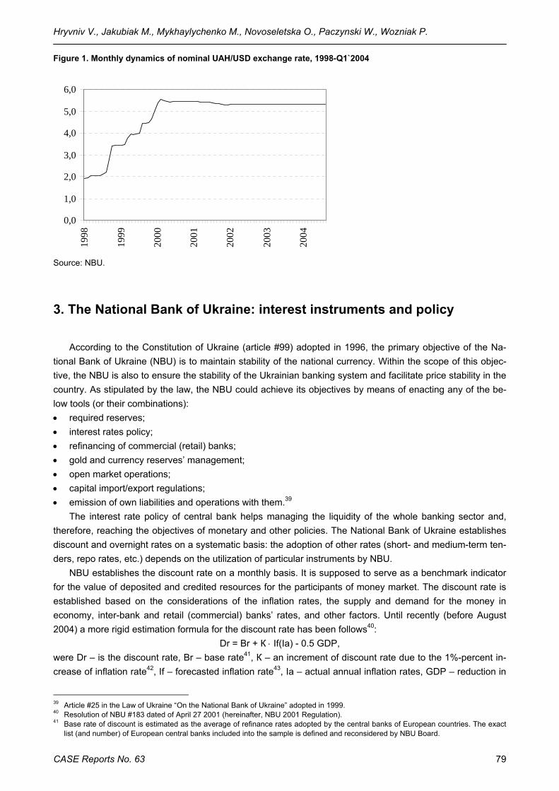
Hryvniv V., Jakubiak M., Mykhaylychenko M., Novoseletska O., Paczynski W., Wozniak P.
CASE Reports No. 63 79
Figure 1. Monthly dynamics of nominal UAH/USD exchange rate, 1998-Q1`2004
0,0
1,0
2,0
3,0
4,0
5,0
6,019
98
1999
2000
2001
2002
2003
2004
Source: NBU.
3. The National Bank of Ukraine: interest instruments and policy
According to the Constitution of Ukraine (article #99) adopted in 1996, the primary objective of the Na-tional Bank of Ukraine (NBU) is to maintain stability of the national currency. Within the scope of this objec-tive, the NBU is also to ensure the stability of the Ukrainian banking system and facilitate price stability in the country. As stipulated by the law, the NBU could achieve its objectives by means of enacting any of the be-low tools (or their combinations): • required reserves; • interest rates policy; • refinancing of commercial (retail) banks; • gold and currency reserves’ management; • open market operations; • capital import/export regulations; • emission of own liabilities and operations with them.39
The interest rate policy of central bank helps managing the liquidity of the whole banking sector and, therefore, reaching the objectives of monetary and other policies. The National Bank of Ukraine establishes discount and overnight rates on a systematic basis: the adoption of other rates (short- and medium-term ten-ders, repo rates, etc.) depends on the utilization of particular instruments by NBU.
NBU establishes the discount rate on a monthly basis. It is supposed to serve as a benchmark indicator for the value of deposited and credited resources for the participants of money market. The discount rate is established based on the considerations of the inflation rates, the supply and demand for the money in economy, inter-bank and retail (commercial) banks’ rates, and other factors. Until recently (before August 2004) a more rigid estimation formula for the discount rate has been follows40:
Dr = Br + К ⋅ If(Ia) - 0.5 GDP, were Dr – is the discount rate, Br – base rate41, К – an increment of discount rate due to the 1%-percent in-crease of inflation rate42, If – forecasted inflation rate43, Ia – actual annual inflation rates, GDP – reduction in
39 Article #25 in the Law of Ukraine “On the National Bank of Ukraine” adopted in 1999. 40 Resolution of NBU #183 dated of April 27 2001 (hereinafter, NBU 2001 Regulation). 41 Base rate of discount is estimated as the average of refinance rates adopted by the central banks of European countries. The exact
list (and number) of European central banks included into the sample is defined and reconsidered by NBU Board.
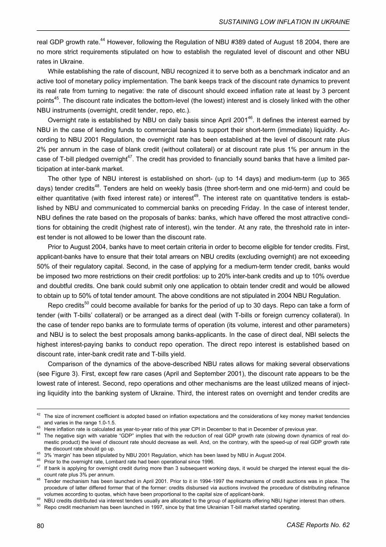
SUSTAINING LOW INFLATION IN UKRAINE
CASE Reports No. 62 80
real GDP growth rate.44 However, following the Regulation of NBU #389 dated of August 18 2004, there are no more strict requirements stipulated on how to establish the regulated level of discount and other NBU rates in Ukraine.
While establishing the rate of discount, NBU recognized it to serve both as a benchmark indicator and an active tool of monetary policy implementation. The bank keeps track of the discount rate dynamics to prevent its real rate from turning to negative: the rate of discount should exceed inflation rate at least by 3 percent points45. The discount rate indicates the bottom-level (the lowest) interest and is closely linked with the other NBU instruments (overnight, credit tender, repo, etc.).
Overnight rate is established by NBU on daily basis since April 200146. It defines the interest earned by NBU in the case of lending funds to commercial banks to support their short-term (immediate) liquidity. Ac-cording to NBU 2001 Regulation, the overnight rate has been established at the level of discount rate plus 2% per annum in the case of blank credit (without collateral) or at discount rate plus 1% per annum in the case of T-bill pledged overnight47. The credit has provided to financially sound banks that have a limited par-ticipation at inter-bank market.
The other type of NBU interest is established on short- (up to 14 days) and medium-term (up to 365 days) tender credits48. Tenders are held on weekly basis (three short-term and one mid-term) and could be either quantitative (with fixed interest rate) or interest49. The interest rate on quantitative tenders is estab-lished by NBU and communicated to commercial banks on preceding Friday. In the case of interest tender, NBU defines the rate based on the proposals of banks: banks, which have offered the most attractive condi-tions for obtaining the credit (highest rate of interest), win the tender. At any rate, the threshold rate in inter-est tender is not allowed to be lower than the discount rate.
Prior to August 2004, banks have to meet certain criteria in order to become eligible for tender credits. First, applicant-banks have to ensure that their total arrears on NBU credits (excluding overnight) are not exceeding 50% of their regulatory capital. Second, in the case of applying for a medium-term tender credit, banks would be imposed two more restrictions on their credit portfolios: up to 20% inter-bank credits and up to 10% overdue and doubtful credits. One bank could submit only one application to obtain tender credit and would be allowed to obtain up to 50% of total tender amount. The above conditions are not stipulated in 2004 NBU Regulation.
Repo credits50 could become available for banks for the period of up to 30 days. Repo can take a form of tender (with T-bills’ collateral) or be arranged as a direct deal (with T-bills or foreign currency collateral). In the case of tender repo banks are to formulate terms of operation (its volume, interest and other parameters) and NBU is to select the best proposals among banks-applicants. In the case of direct deal, NBI selects the highest interest-paying banks to conduct repo operation. The direct repo interest is established based on discount rate, inter-bank credit rate and T-bills yield.
Comparison of the dynamics of the above-described NBU rates allows for making several observations (see Figure 3). First, except few rare cases (April and September 2001), the discount rate appears to be the lowest rate of interest. Second, repo operations and other mechanisms are the least utilized means of inject-ing liquidity into the banking system of Ukraine. Third, the interest rates on overnight and tender credits are
42 The size of increment coefficient is adopted based on inflation expectations and the considerations of key money market tendencies
and varies in the range 1.0-1.5. 43 Here inflation rate is calculated as year-to-year ratio of this year CPI in December to that in December of previous year. 44 The negative sign with variable “GDP” implies that with the reduction of real GDP growth rate (slowing down dynamics of real do-
mestic product) the level of discount rate should decrease as well. And, on the contrary, with the speed-up of real GDP growth rate the discount rate should go up.
45 3% ‘margin’ has been stipulated by NBU 2001 Regulation, which has been laxed by NBU in August 2004. 46 Prior to the overnight rate, Lombard rate had been operational since 1996. 47 If bank is applying for overnight credit during more than 3 subsequent working days, it would be charged the interest equal the dis-
count rate plus 3% per annum. 48 Tender mechanism has been launched in April 2001. Prior to it in 1994-1997 the mechanisms of credit auctions was in place. The
procedure of latter differed former that of the former: credits disbursed via auctions involved the procedure of distributing refinance volumes according to quotas, which have been proportional to the capital size of applicant-bank.
49 NBU credits distributed via interest tenders usually are allocated to the group of applicants offering NBU higher interest than others. 50 Repo credit mechanism has been launched in 1997, since by that time Ukrainian T-bill market started operating.
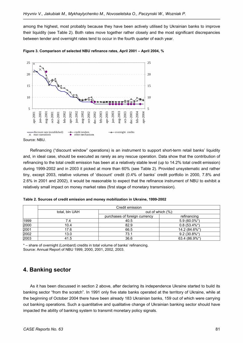
Hryvniv V., Jakubiak M., Mykhaylychenko M., Novoseletska O., Paczynski W., Wozniak P.
CASE Reports No. 63 81
among the highest, most probably because they have been actively utilised by Ukrainian banks to improve their liquidity (see Table 2). Both rates move together rather closely and the most significant discrepancies between tender and overnight rates tend to occur in the fourth quarter of each year.
Figure 3. Comparison of selected NBU refinance rates, April 2001 – April 2004, %
5
10
15
20
25
apr-2
001
jun-
2001
aug-
2001
oct-2
001
dec-
2001
feb-
2002
apr-2
002
jun-
2002
aug-
2002
oct-2
002
dec-
2002
feb-
2003
apr-2
003
jun-
2003
aug-
2003
oct-2
003
dec-
2003
feb-
2004
apr-2
004
5
10
15
20
25
discount rate (established) credit tenders overnight creditsrepo operations other mechanisms
Source: NBU.
Refinancing (“discount window” operations) is an instrument to support short-term retail banks’ liquidity and, in ideal case, should be executed as rarely as any rescue operation. Data show that the contribution of refinancing to the total credit emission has been at a relatively stable level (up to 14.2% total credit emission) during 1999-2002 and in 2003 it picked at more than 60% (see Table 2). Provided unsystematic and rather tiny, except 2003, relative volumes of ‘discount’ credit (0.4% of banks’ credit portfolio in 2000, 7.8% and 2.6% in 2001 and 2002), it would be reasonable to expect that the refinance instrument of NBU to exhibit a relatively small impact on money market rates (first stage of monetary transmission).
Table 2. Sources of credit emission and money mobilization in Ukraine, 1999-2002
Credit emission out of which (%):
total, bln UAH
purchases of foreign currency refinancing 1999 7.4 40.5 5.9 (60.0%*) 2000 10.4 82.9 0.8 (53.4%*) 2001 17.6 66.5 14.2 (84.6%*) 2002 13.0 73.1 9.2 (30.8%*) 2003 41.5 36.6 63.4 (86.9%*)
* – share of overnight (Lombard) credits in total volume of banks’ refinancing. Source: Annual Report of NBU 1999, 2000, 2001, 2002, 2003.
4. Banking sector
As it has been discussed in section 2 above, after declaring its independence Ukraine started to build its banking sector “from the scratch”. In 1991 only five state banks operated at the territory of Ukraine, while at the beginning of October 2004 there have been already 183 Ukrainian banks, 159 out of which were carrying out banking operations. Such a quantitative and qualitative change of Ukrainian banking sector should have impacted the ability of banking system to transmit monetary policy signals.

SUSTAINING LOW INFLATION IN UKRAINE
CASE Reports No. 62 82
At the end of September 2004 two state banks and 19 (out of which only 7 have a 100% of foreign capital) foreign banks operated at the market of Ukraine. As of October 1, the share of foreign capital in the total amount of authorised capital of Ukrainian banks has been slightly exceeding 10%, which has had a downward tendency over the last five years. Therefore, one could conclude that the competition at the Ukrainian banking market (in particular, between the foreign and Ukrainian banks) has been reducing over time.
The reduced competition in the banking sector of Ukraine could be a consequence of sector consolida-tion, especially as concerns the Ukrainian banks, which are required to raise their capitalisation level gradu-ally. The level of concentration among 10 largest Ukrainian banks remained almost without a change (55.3% of total sector assets in December 2000 and 54.9% in June 2004), while the concentration among 25 largest banks increased slightly (from 71.4% in December 2000 to 72.3% in June 2004). Among the top-10 banks, those with the high volume of assets, there are Savings bank, Aval, Ukrsotsbank, Ukreximbank, Prominvest-bank and Privatbank, out of which two banks are state and two more have been formerly state-owned. Over last several years the “leading” group of banks remained stable, which could suggest us that the Ukrainian banking market is segmented, that is divided into several groups with the sounder and more financially solid banks having higher chances to maintain operational at the market.
During 2001-2003 credits have expanded significantly in Ukraine, so that the average growth rate for the period was slightly over 50%. Although being positive, the tendency raises much a number of concerns, one of which is the quality of assets. In 2000-2002 the share of non-performing (substandard, doubtful, and loss) loans reduced from 29.6% of total loans to 21.9%. As of June 2004, the share of non-performing loans con-stituted 27.5%, which is not compatible to the preceding dynamics, since NBU introduced new loan classifi-cation rules in 2003. The international comparison shows that this indicator is relatively higher that in other transition countries, in which this indicator does not exceed 5% (Russia, Czech Republic, Croatia, Bulgaria, Lithuania, Latvia, Hungary, Estonia, etc.).
The soundness of Ukrainian banks, at least as far as the capital adequacy ratio is concerned, remained unchanged: from 15.5 in 2000 to 15.2 in June 2004. Bigger banks are more capitalised that the other, which makes them a major source of injecting new credits into economy. As proven by Prof. Karcheva (NBU Her-ald, October 2004), only higher capitalised Ukrainian banks with the bigger share of attracted long-term household deposits are capable of increasing credits and investments into economy. Therefore, the credit channel of monetary transmission would be limited to these banks only in Ukraine.
Figure 4. Ukrainian banks’ liabilities and credit portfolio, 1998-2003, annual, bln UAH
0
1020
30
40
5060
70
1998
1999
2000
2001
2002
2003
total deposits, bln UAH total credits, bln UAH
Source: NBU.
In 2001-2003 the Ukrainian banking sector experienced a credit boom. Over three last years the size of Ukrainian banks’ liabilities almost tripled (see Figure 4). As of October 1 2004 the share of time deposits in total
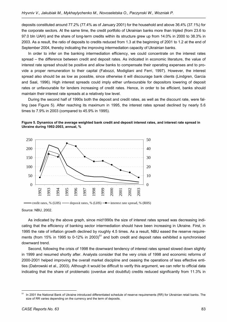
Hryvniv V., Jakubiak M., Mykhaylychenko M., Novoseletska O., Paczynski W., Wozniak P.
CASE Reports No. 63 83
deposits constituted around 77.2% (77.4% as of January 2001) for the household and above 36.4% (37.1%) for the corporate sectors. At the same time, the credit portfolio of Ukrainian banks more than tripled (from 23.6 to 97.0 bln UAH) and the share of long-term credits within its structure grew up from 14.0% in 2000 to 38.3% in 2003. As a result, the ratio of deposits to credits reduced from 1.3 at the beginning of 2001 to 1.2 at the end of September 2004, thereby indicating the improving intermediation capacity of Ukrainian banks.
In order to infer on the banking intermediation efficiency, we could concentrate on the interest rates spread – the difference between credit and deposit rates. As indicated in economic literature, the value of interest rate spread should be positive and allow banks to compensate their operating expenses and to pro-vide a proper remuneration to their capital (Fabozzi, Modigliani and Ferri, 1997). However, the interest spread also should be as low as possible, since otherwise it will discourage bank clients (Lindgren, Garcia and Saal, 1996). High interest spreads could imply either unfavourable for depositors lowering of deposit rates or unfavourable for lenders increasing of credit rates. Hence, in order to be efficient, banks should maintain their interest rate spreads at a relatively low level.
During the second half of 1990s both the deposit and credit rates, as well as the discount rate, were fal-ling (see Figure 5). After reaching its maximum in 1995, the interest rates spread declined by nearly 5.6 times to 7.9% in 2003 (compared to 45.9% in 1995).
Figure 5. Dynamics of the average weighted bank credit and deposit interest rates, and interest rate spread in Ukraine during 1992-2003, annual, %
0
50
100
150
200
250
1992
1993
1994
1995
1996
1997
1998
1999
2000
2001
2002
2003
0
10
20
30
40
50
credit rates, % (LHS) deposit rates, % (LHS) interest rate spread, % (RHS)
Source: NBU, 2002.
As indicated by the above graph, since mid1990s the size of interest rates spread was decreasing indi-cating that the efficiency of banking sector intermediation should have been increasing in Ukraine. First, in 1995 the rate of inflation growth declined by roughly 4.5 times. As a result, NBU eased the reserve require-ments (from 15% in 1995 to 0-12% in 2003)51 and both credit and deposit rates exhibited a synchronised downward trend.
Second, following the crisis of 1998 the downward tendency of interest rates spread slowed down slightly in 1999 and resumed shortly after. Analysts consider that the very crisis of 1998 and economic reforms of 2000-2001 helped improving the overall market discipline and ceasing the operations of less effective enti-ties (Dabrowski et al., 2003). Although it would be difficult to verify this argument, we can refer to official data indicating that the share of problematic (overdue and doubtful) credits reduced significantly from 11.3% in
51 In 2001 the National Bank of Ukraine introduced differentiated schedule of reserve requirements (RR) for Ukrainian retail banks. The
size of RR varies depending on the currency and the term of deposits.
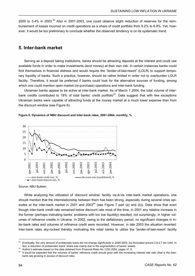
SUSTAINING LOW INFLATION IN UKRAINE
CASE Reports No. 62 84
2000 to 3.4% in 2003.52 Also in 2001-2003, one could observe slight reduction of reserves for the reim-bursement of losses incurred on credit operations as a share of credit portfolio from 9.2% to 6.8%. Yet, how-ever, it would be too preliminary to conclude whether the observed tendency is on its systematic trend.
5. Inter-bank market
Serving as a deposit taking institutions, banks should be attracting deposits at the interest and could use available funds in order to make investments (lend money) at their own risk. In certain instances banks could find themselves in financial distress and would require the “lender-of-last-resort” (LOLR) to support tempo-rary liquidity of banks. Such a practice, however, should be rather limited in order not to overburden LOLR facility. Therefore, it would be preferred if banks could look for the alternative sources of funding, among which one could mention open market (re-purchase) operations and inter-bank funding.
Ukrainian banks appear to be active at inter-bank market. As of March 1 2004, the total volume of inter-bank credits contributed to 18% of total banks’ credit portfolio53. Data suggest that with few exceptions Ukrainian banks were capable of attracting funds at the money market at a much lower expense than from the discount window (see Figure 6).
Figure 6. Dynamics of NBU discount and inter-bank rates, 2001-2004, monthly, %
0
5
10
15
20
25
30
apr-2
001
jul-2
001
oct-2
001
jan-
2002
apr-2
002
jul-2
002
oct-2
002
jan-
2003
apr-2
003
jul-2
003
oct-2
003
jan-
2004
inter-bank credit rate, % discount rate (established), %inter-bank deposit rate, %
Source: NBU Bulletin.
While analyzing the utilization of ‘discount window’ facility vis-à-vis inter-bank market operations, one should mention that the interrelationship between them has been strong, especially during several crisis epi-sodes at the inter-bank market in 2001 and 200354 (see Figure 7 part (a) and (b)). Data show that even though inter-bank credit rate remained below discount rate most of the time, in 2001 any relative increase in the former (perhaps indicating banks’ problems with too low liquidity) resulted, not surprisingly, in higher vol-umes of refinance credits in Ukraine. In 2002, owing to the deflationary period, no significant changes in in-ter-bank rates and volumes of refinance credit were recorded. However, in late 2003 the situation reverted: inter-bank rates sky-rocked thereby motivating the retail banks to utilize the ‘lender-of-last-resort’ facility
52 Eventually, the very amount of problematic loans did not change significantly in 2000-2003, but fluctuated around 2.6-2.7 bln UAH. In
fact, a reduction of problematic loans’ share was mainly due to the augmentation of banks’ assets. 53 Author’s estimate based on the data obtained from Financial Risks No 1(35) 2004, pages VI, X. 54 It would be expected that the volumes of banks’ refinance credit should grow with the increasing interest rate ratio (that is the inter-
bank rate growing in excess of discount rate).
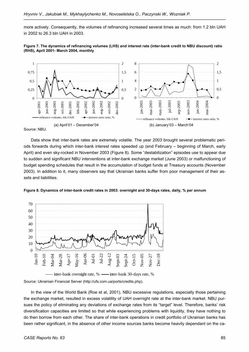
Hryvniv V., Jakubiak M., Mykhaylychenko M., Novoseletska O., Paczynski W., Wozniak P.
CASE Reports No. 63 85
more actively. Consequently, the volumes of refinancing increased several times as much: from 1.2 bln UAH in 2002 to 26.3 bln UAH in 2003.
Figure 7. The dynamics of refinancing volumes (LHS) and interest rate (inter-bank credit to NBU discount) ratio (RHS), April 2001- March 2004, monthly
(a) April’01 – December’04 (b) January’03 – March’04 Source: NBU.
Data show that inter-bank rates are extremely volatile. The year 2003 brought several problematic peri-ods forwards during which inter-bank interest rates speeded up (end February – beginning of March, early April) and even sky-rocked in November 2003 (Figure 8). Some “destabilization” episodes use to appear due to sudden and significant NBU interventions at inter-bank exchange market (June 2003) or malfunctioning of budget spending schedules that result in the accumulation of budget funds at Treasury accounts (November 2003). In addition to it, many observers say that Ukrainian banks suffer from poor management of their as-sets and liabilities.
Figure 8. Dynamics of inter-bank credit rates in 2003: overnight and 30-days rates, daily, % per annum
010203040506070
Jan-
10
Feb-
10
Mar
-04
Mar
-28
Apr
-17
May
-16
Jun-
06
Jul-0
1
Jul-2
2
Aug
-12
Sept
-03
Sept
-24
Oct
-15
Nov
-05
Nov
-27
Dec
-18
inter-bank overnight rate, % inter-bank 30-days rate, %
Source: Ukrainian Financial Server (http://ufs.com.ua/ports/credits.php).
In the view of the World Bank (Roe et al, 2001), NBU excessive regulations, especially those pertaining the exchange market, resulted in excess volatility of UAH overnight rate at the inter-bank market. NBU pur-sues the policy of eliminating any deviations of exchange rates from its “target” level. Therefore, banks’ risk diversification capacities are limited so that while experiencing problems with liquidity, they have nothing to do then borrow from each other. The share of inter-bank operations in credit portfolio of Ukrainian banks has been rather significant, in the absence of other income sources banks become heavily dependant on the ca-
0
0,25
0,5
0,75
1
apr-2
001
jun-
2001
aug-
2001
oct-2
001
dec-
2001
feb-
2002
apr-2
002
jun-
2002
aug-
2002
oct-2
002
dec-
2002
0
0,5
1
1,5
2
refinance volumes, bln UAH interest rates ratio, %
0
2
4
6
8
jan-
2003
mar
-200
3
may
-200
3
jul-2
003
sep-
2003
nov-
2003
jan-
2004
mar
-200
4
0
0,5
1
1,5
2
refinance volumes, bln UAH interest rates ratio, %
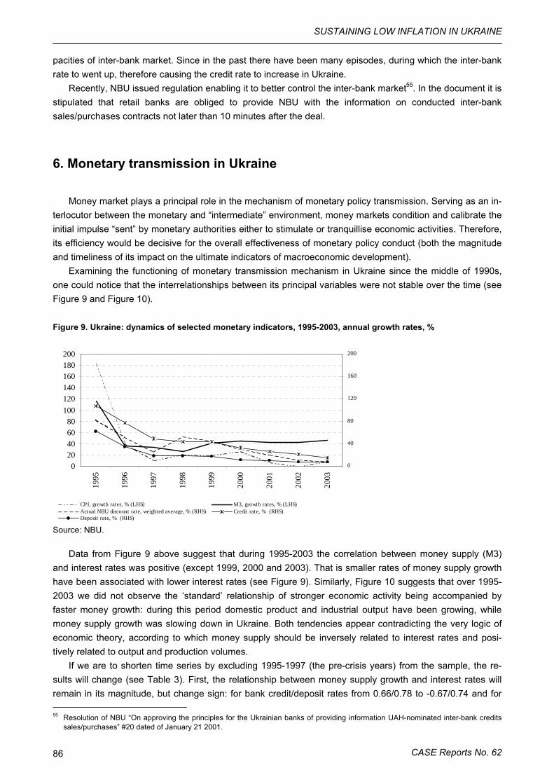
SUSTAINING LOW INFLATION IN UKRAINE
CASE Reports No. 62 86
pacities of inter-bank market. Since in the past there have been many episodes, during which the inter-bank rate to went up, therefore causing the credit rate to increase in Ukraine.
Recently, NBU issued regulation enabling it to better control the inter-bank market55. In the document it is stipulated that retail banks are obliged to provide NBU with the information on conducted inter-bank sales/purchases contracts not later than 10 minutes after the deal.
6. Monetary transmission in Ukraine
Money market plays a principal role in the mechanism of monetary policy transmission. Serving as an in-terlocutor between the monetary and “intermediate” environment, money markets condition and calibrate the initial impulse “sent” by monetary authorities either to stimulate or tranquillise economic activities. Therefore, its efficiency would be decisive for the overall effectiveness of monetary policy conduct (both the magnitude and timeliness of its impact on the ultimate indicators of macroeconomic development).
Examining the functioning of monetary transmission mechanism in Ukraine since the middle of 1990s, one could notice that the interrelationships between its principal variables were not stable over the time (see Figure 9 and Figure 10).
Figure 9. Ukraine: dynamics of selected monetary indicators, 1995-2003, annual growth rates, %
020406080
100120140160180200
1995
1996
1997
1998
1999
2000
2001
2002
2003
0
40
80
120
160
200
CPI, growth rates, % (LHS) M3, growth rates, % (LHS)Actual NBU discount rate, weighted average, % (RHS) Credit rate, % (RHS)Deposit rate, % (RHS)
Source: NBU.
Data from Figure 9 above suggest that during 1995-2003 the correlation between money supply (M3) and interest rates was positive (except 1999, 2000 and 2003). That is smaller rates of money supply growth have been associated with lower interest rates (see Figure 9). Similarly, Figure 10 suggests that over 1995-2003 we did not observe the ‘standard’ relationship of stronger economic activity being accompanied by faster money growth: during this period domestic product and industrial output have been growing, while money supply growth was slowing down in Ukraine. Both tendencies appear contradicting the very logic of economic theory, according to which money supply should be inversely related to interest rates and posi-tively related to output and production volumes.
If we are to shorten time series by excluding 1995-1997 (the pre-crisis years) from the sample, the re-sults will change (see Table 3). First, the relationship between money supply growth and interest rates will remain in its magnitude, but change sign: for bank credit/deposit rates from 0.66/0.78 to -0.67/0.74 and for 55 Resolution of NBU “On approving the principles for the Ukrainian banks of providing information UAH-nominated inter-bank credits
sales/purchases” #20 dated of January 21 2001.
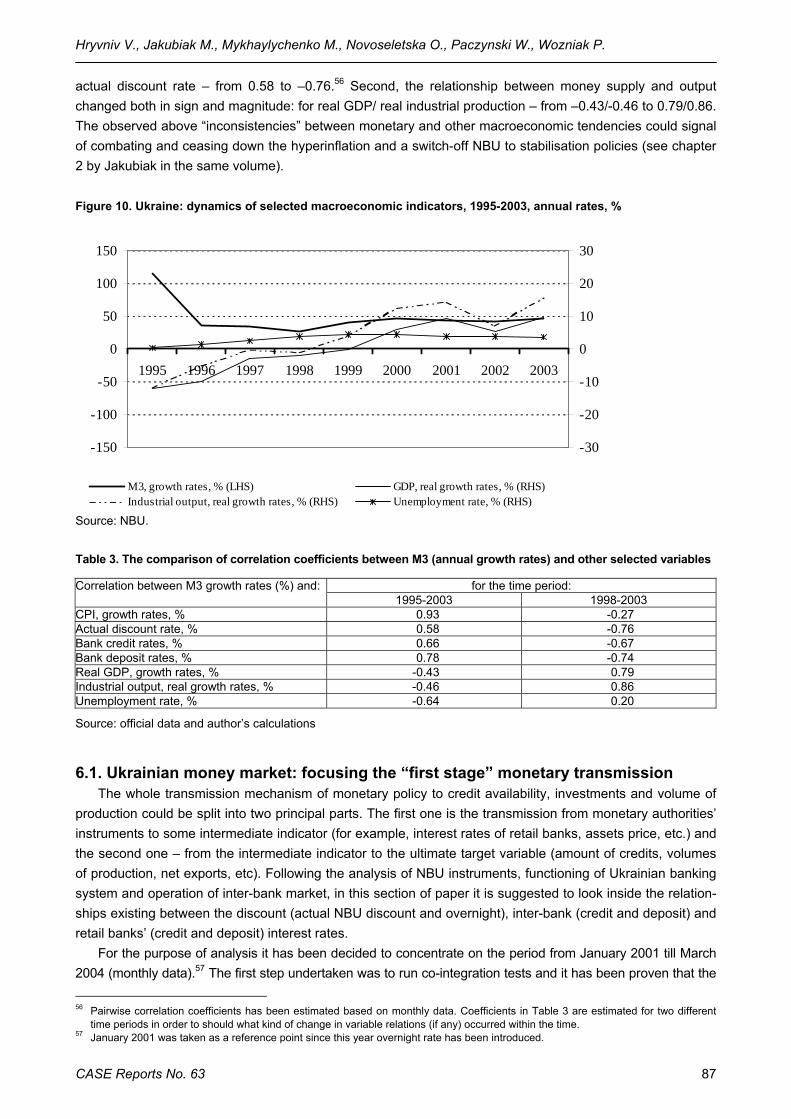
Hryvniv V., Jakubiak M., Mykhaylychenko M., Novoseletska O., Paczynski W., Wozniak P.
CASE Reports No. 63 87
actual discount rate – from 0.58 to –0.76.56 Second, the relationship between money supply and output changed both in sign and magnitude: for real GDP/ real industrial production – from –0.43/-0.46 to 0.79/0.86. The observed above “inconsistencies” between monetary and other macroeconomic tendencies could signal of combating and ceasing down the hyperinflation and a switch-off NBU to stabilisation policies (see chapter 2 by Jakubiak in the same volume).
Figure 10. Ukraine: dynamics of selected macroeconomic indicators, 1995-2003, annual rates, %
-150
-100
-50
0
50
100
150
1995 1996 1997 1998 1999 2000 2001 2002 2003
-30
-20
-10
0
10
20
30
M3, growth rates, % (LHS) GDP, real growth rates, % (RHS)Industrial output, real growth rates, % (RHS) Unemployment rate, % (RHS)
Source: NBU.
Table 3. The comparison of correlation coefficients between M3 (annual growth rates) and other selected variables
for the time period: Correlation between M3 growth rates (%) and: 1995-2003 1998-2003
CPI, growth rates, % 0.93 -0.27 Actual discount rate, % 0.58 -0.76 Bank credit rates, % 0.66 -0.67 Bank deposit rates, % 0.78 -0.74 Real GDP, growth rates, % -0.43 0.79 Industrial output, real growth rates, % -0.46 0.86 Unemployment rate, % -0.64 0.20
Source: official data and author’s calculations
6.1. Ukrainian money market: focusing the “first stage” monetary transmission The whole transmission mechanism of monetary policy to credit availability, investments and volume of
production could be split into two principal parts. The first one is the transmission from monetary authorities’ instruments to some intermediate indicator (for example, interest rates of retail banks, assets price, etc.) and the second one – from the intermediate indicator to the ultimate target variable (amount of credits, volumes of production, net exports, etc). Following the analysis of NBU instruments, functioning of Ukrainian banking system and operation of inter-bank market, in this section of paper it is suggested to look inside the relation-ships existing between the discount (actual NBU discount and overnight), inter-bank (credit and deposit) and retail banks’ (credit and deposit) interest rates.
For the purpose of analysis it has been decided to concentrate on the period from January 2001 till March 2004 (monthly data).57 The first step undertaken was to run co-integration tests and it has been proven that the
56 Pairwise correlation coefficients has been estimated based on monthly data. Coefficients in Table 3 are estimated for two different
time periods in order to should what kind of change in variable relations (if any) occurred within the time. 57 January 2001 was taken as a reference point since this year overnight rate has been introduced.
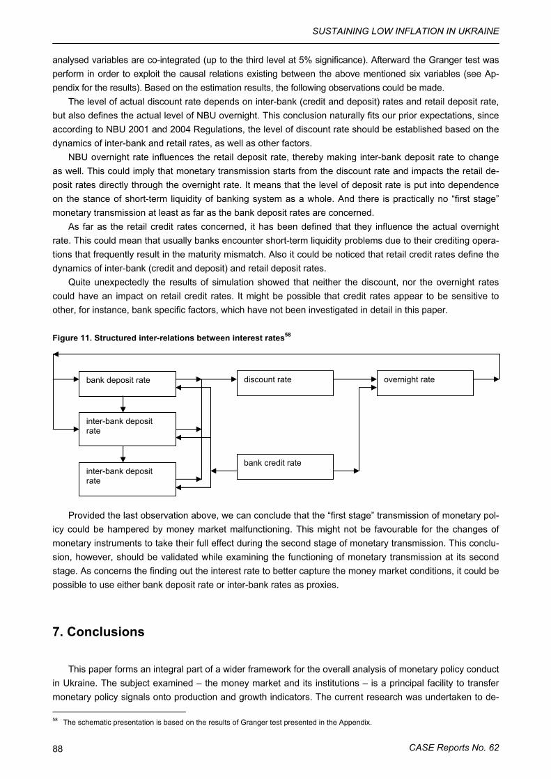
SUSTAINING LOW INFLATION IN UKRAINE
CASE Reports No. 62 88
analysed variables are co-integrated (up to the third level at 5% significance). Afterward the Granger test was perform in order to exploit the causal relations existing between the above mentioned six variables (see Ap-pendix for the results). Based on the estimation results, the following observations could be made.
The level of actual discount rate depends on inter-bank (credit and deposit) rates and retail deposit rate, but also defines the actual level of NBU overnight. This conclusion naturally fits our prior expectations, since according to NBU 2001 and 2004 Regulations, the level of discount rate should be established based on the dynamics of inter-bank and retail rates, as well as other factors.
NBU overnight rate influences the retail deposit rate, thereby making inter-bank deposit rate to change as well. This could imply that monetary transmission starts from the discount rate and impacts the retail de-posit rates directly through the overnight rate. It means that the level of deposit rate is put into dependence on the stance of short-term liquidity of banking system as a whole. And there is practically no “first stage” monetary transmission at least as far as the bank deposit rates are concerned.
As far as the retail credit rates concerned, it has been defined that they influence the actual overnight rate. This could mean that usually banks encounter short-term liquidity problems due to their crediting opera-tions that frequently result in the maturity mismatch. Also it could be noticed that retail credit rates define the dynamics of inter-bank (credit and deposit) and retail deposit rates.
Quite unexpectedly the results of simulation showed that neither the discount, nor the overnight rates could have an impact on retail credit rates. It might be possible that credit rates appear to be sensitive to other, for instance, bank specific factors, which have not been investigated in detail in this paper.
Figure 11. Structured inter-relations between interest rates58
Provided the last observation above, we can conclude that the “first stage” transmission of monetary pol-icy could be hampered by money market malfunctioning. This might not be favourable for the changes of monetary instruments to take their full effect during the second stage of monetary transmission. This conclu-sion, however, should be validated while examining the functioning of monetary transmission at its second stage. As concerns the finding out the interest rate to better capture the money market conditions, it could be possible to use either bank deposit rate or inter-bank rates as proxies.
7. Conclusions
This paper forms an integral part of a wider framework for the overall analysis of monetary policy conduct in Ukraine. The subject examined – the money market and its institutions – is a principal facility to transfer monetary policy signals onto production and growth indicators. The current research was undertaken to de- 58 The schematic presentation is based on the results of Granger test presented in the Appendix.
bank deposit rate
bank credit rate inter-bank deposit rate
inter-bank deposit rate
discount rate overnight rate
Hryvniv V., Jakubiak M., Mykhaylychenko M., Novoseletska O., Paczynski W., Wozniak P.
CASE Reports No. 63 89
fine whether money market conditions has been favourable for the effective monetary policy conduct (“first stage” of transmission).
As concerns the monetary transmission, we have seen that during 1995-2003 no standard relations be-tween monetary and other macroeconomic variables (GDP, volumes of industrial production, unemployment, etc.) has been observed. On the one hand, this could signal of the switch in NBU policy in 1998-1999: from combating hyperinflation towards more effective stabilisation policies. On the other, this imply, most proba-bly, the malfunctioning of the very money market not being able to properly transmit the changes of monetary instruments to economy.
The analysis of “first stage” monetary transmission indicated that unlike the other rates, retail credit rates remain exogenous to the whole array of different interest instruments. Most probably, we could attribute this to other factors having more influence on bank credit rates. Among them one could mention bank specific, for example, competition, bank soundness, assets quality and others, which could significantly hamper the efficiency of banking sector as a whole.
The exogenity of credit rates could mean that monetary authorities are not capable to influence them in the desired manner. Changes in credit availability might be inadequate provided the changes of monetary instruments and, therefore, costly in its economic sense. However, to better shed the light on this we should switch to the analysis of “second stage” of monetary transmission.
Appendix. Results of Granger causality test
Sample: 2001:01 2004:03 Lags: 2 Null Hypothesis: Obs F-Statistic Probability ONA does not Granger Cause DA 27 27.6011 1.0E-06 DA does not Granger Cause ONA 1.98554 0.16116 CBC does not Granger Cause DA 34 0.57968 0.56643 DA does not Granger Cause CBC 1.33380 0.27916 CBD does not Granger Cause DA 34 0.35751 0.70246 DA does not Granger Cause CBD 5.89218 0.00712 IBD does not Granger Cause DA 34 1.10518 0.34470 DA does not Granger Cause IBD 7.50742 0.00236 IBC does not Granger Cause DA 34 1.11133 0.34274 DA does not Granger Cause IBC 3.61021 0.03981 CBC does not Granger Cause ONA 27 0.02721 0.97319 ONA does not Granger Cause CBC 3.23446 0.05869 CBD does not Granger Cause ONA 27 4.71550 0.01976 ONA does not Granger Cause CBD 0.99383 0.38617 IBD does not Granger Cause ONA 27 3.55892 0.04580 ONA does not Granger Cause IBD 0.97950 0.39128 IBC does not Granger Cause ONA 27 1.37906 0.27274 ONA does not Granger Cause IBC 0.15088 0.86084 CBD does not Granger Cause CBC 37 4.70066 0.01622 CBC does not Granger Cause CBD 0.36300 0.69842 IBD does not Granger Cause CBC 37 3.71253 0.03548 CBC does not Granger Cause IBD 1.50259 0.23784 IBC does not Granger Cause CBC 37 3.71232 0.03549 CBC does not Granger Cause IBC 1.46964 0.24512 IBD does not Granger Cause CBD 37 5.95061 0.00635 CBD does not Granger Cause IBD 1.97971 0.15467 IBC does not Granger Cause CBD 37 9.51180 0.00057 CBD does not Granger Cause IBC 4.53631 0.01843 IBC does not Granger Cause IBD 37 5.36762 0.00977 IBD does not Granger Cause IBC 0.42415 0.65795 where CBC – retail credit rate (average weighted), CBD – retail deposit rate (average weighted), IBD – inter-bank deposit rate, IBC – inter-bank credit rate, DA – actual discount rate, ONA – actual overnight rate.
SUSTAINING LOW INFLATION IN UKRAINE
CASE Reports No. 62 90
References
Alexander, W. E., and F. Caramazza (1994) Money Versus Credit: The Role of Banks in the Monetary Transmission Process, in Frameworks for Monetary Stability, ed. by Tomas J.T. Balino and Carlo Cottarelli, pp. 379-422. International Monetary Fund: Washington.
Bernanke, B., and M. Gertler (1995) Inside the Black Box: The Credit Channel of Monetary Policy Transmission, Journal of Economic Perspectives, Vol. 9 (Fall), pp 27-48.
Brunner, K., and A. M. Meltzer (1998) Money and Credit in the Monetary Transmission Process, Ameri-can Economic Review, Vol. 28 (May), pp. 446-51.
Cecchetti, S. (1995) Distinguishing Theories of Monetary Transmission Mechanism, Federal Reserve Bank of St. Louis, Review 77 (May-June), pp. 83-97.
Cottarelli, C., and A. Kourelis (1994) Financial Structure, Bank Lending Rates, and the Transmission Mechanism of Monetary Policy, Staff Papers, International Monetary Fund, Vol. 41 (December), pp 587-623.
Dabrowski, M. and M. Jakubiak (2003) The Sources of Economic Growth in Ukraine after 1998 Currency Crisis and the Country's Prospects, CASE Reports.
Dimsdale, N. (1994). Banks, Capital Markets, and the Monetary Transmission Mechanism, Oxford Re-view of Economic Policy, Vol. 10 (Winter), pp. 34-48.
Fabozzi F. J., Modigliani F. and M. G. Ferri (1997) Foundations of Financial Markets and Institutions. Second edition, Prentice Hall.
Fitch T. P. (1997) Dictionary of Banking Terms, Third Edition, Barron’s. Hubbard, G. R. (1995) Is There a ‘Credit Channel’ of Monetary Policy?, Federal Reserve Bank of St.
Louis, Review 77 (May-June), pp. 63-74. IMF (1998). International Financial Statistics. Yearbook. IMF: Washington. Karcheva, G. (2004) Modelling the Investment Activity of Banks, NBU Herald (October), pp. 11-15. Lindgren C., Garcia G. and M. I. Saal (1996) Bank Soundness and Macroeconomic Policy, International
Monetary Fund. Mishkin F. S. (1997) The Economics of Money, Banking and Financial Markets. Fifth Edition, Addison
Wesley. Montes-Negret F., and L. Papi (1995) Are Bank Interest Rate Spreads Too High?, World Bank Working
Papers. Ramey V. (1993) How Important is Credit Channel in the Transmission of Monetary Policy?, Carnegie-
Rochester Conference Series on Public Policy, Vol. 39, pp 1-45. Roe A., Vlasenko Y., Zhyliaev I., Olenchyk A., Pitchi S., Prigozhina A., and C. Forgash (2001) Ukraine. Fi-
nancial Sector and Economy. New Policy Agenda. The International Bank of Reconstruction and Development. Taylor, J. (1995) The Monetary Transmission Mechanism: An Empirical Framework, Journal of Economic
Perspectives, Vol. 9 (Fall), pp 11-26.
Periodicals: Bulletin of NBU, 1999-2002. Finansovye Riski, 1998-2001. NBU Herald, 2000-2002.
Hryvniv V., Jakubiak M., Mykhaylychenko M., Novoseletska O., Paczynski W., Wozniak P.
CASE Reports No. 63 91
Chapter 7: Monetary Transmission Mechanism in Ukraine: A VAR Approach
Mykyta Mykhaylychenko, Volodymyr Hryniv, Wojciech Paczyński
1. Introduction
This work attempts to apply a well established Vector Autoregression (VAR) methodology to study mone-tary transmission mechanism in Ukraine. Various versions of such studies are perhaps the most common approach in empirical transmission literature in the world. Examples of work in this category include, Leeper et al. (1998), Christiano et al. (2000) and Peersman and Smets (2001). However, to our knowledge, this ap-proach has not been widely applied in Ukraine up to now. This paper attempts to fill this gap by looking at VAR evidence on the monetary transmission process in Ukraine.
Throughout the paper, a benchmark VAR specification, proposed by Peersman and Smets (2001), is used to uncover responses of main Ukrainian macroeconomic variables to interest rate innovation, treated as a monetary policy shock. It is discovered that these responses are present, at least as regards inflation, and the general picture emerging is not at odds with evidence from other countries (e.g. the euro-zone and USA).
Another attribute of this research is that we try to estimate VAR in two “dimensions”. Firstly, several dif-ferent interest rates are used as monetary policy indicators, including NBU’s discount rate, interbank rate and loan interest rate of commercial banks. Secondly, core inflation indicators as well as ordinary CPI, calculated by the Ukrainian State Statistics Committee, are involved in the evaluation. It is revealed that the results for VARs with different interest rates are similar with slight differences. There are no clear cut results concerning the choice of core CPI or standard CPI as a better indicator to be potentially controlled by interest rate changes, though some core inflation indices appear to be more appropriate in this respect.
The paper is organized as follows. The second section offers a brief historical survey on monetary transmission research in Ukraine. Section 3 is devoted to the benchmark VAR model and data description and to the presentation of results based on impulse response functions. Section 4 introduces analysis of variance decomposition and discusses some other robustness checks. Conclusions are in section 5.
2. An overview of empirical work on monetary transmission in Ukraine
Up till now there has been relatively little research on monetary transmission mechanism in Ukraine. Ex-amples of work studying various aspects of transmission include Doroshenko (2001), Tyrkalo and Adamyk (1999), Zaderey (2003), Novoseletska (2005), Shevchuk (2001). Below we provide a concise overview of this literature signaling major approaches that have been taken and summarizing the main findings.
SUSTAINING LOW INFLATION IN UKRAINE
CASE Reports No. 62 92
Firstly, there is a relatively large literature dealing with relations between monetary indicators and other macroeconomic variables. Tyrkalo and Adamyk (1999) and Doroshenko (2001) consider relations between both money supply and inflation and between money supply and GDP. The findings confirm a long-run rela-tionship between money growth and inflation (as one would expect). The period of money expansion and high inflation in the decade of the 1990s was accompanied by contraction of output. Novoseletska (2005) also discusses these issues making note of the break point in the statistical relationship. In the more recent period of financial stability (1999-2003) rising monetary aggregates were accompanied by falling inflation and a rebound of output. Clearly, there are major differences between long-run and short-term effects of money expansion. Bilan (2002 and 2003), Bilan and Siliverstovs (2004), and Leheyda (2004) are examples of recent work studying various aspects of impact of monetary aggregates on other variables and in particular of infla-tion determinants.
Bilan (2003) studies the existence, strength and importance of the ‘liquidity effect’, i.e. fall of interest rates (interbank) in response to money expansion. The study finds the effect to be present and – more im-portantly – to remain in place for a relatively long period. It would thus provide some evidence supporting the view that interest rate channel of monetary transmission has some power – at least as far as the first stage of the transmission is concerned (i.e. an influence of money expansion on market interest rates).
Doroshenko (2001) considers some aspects of exchange rate channel. The results indicate that ex-change rate fluctuations had very limited impact on trade flows over the period 1994-1998. The paper further identifies other factors (different from exchange rates) that shape foreign trade dynamics. The results can be interpreted as giving some support to the hypothesis that exchange rate channel of monetary policy trans-mission can be relatively weak as there appears to be little impact from exchange rates to the trade balance. The suggested explanations include administrative influences in foreign trade. The period from 1999 onward was characterized by nominal stability of exchange rate (de facto peg), so that the potential importance of the exchange rate channel of monetary transmission is hard to test.
Another aspect of this channel – pass-through from exchange rates to prices – was briefly considered by Novoseletska and Myhaylychenko (2004). Authors note that nominal exchange rate stability could contribute to moderate growth rates of prices during the last few years.
There is not too much work directly addressing the relative importance of the credit channel of transmis-sion. Kryshko (2001) is one example concentrating on the first stage of transmission, i.e. the behavior of commercial banks in response to monetary policy actions. The evidence provided by Zaderey (2003) sug-gests a rather weak potential for broad credit channel of monetary transmission. Novoseletska (2004) pro-vide institutional analysis that can be helpful in assessing the potential importance of the channel.
Finally, it is worth mentioning that some work using simple structural approaches to modeling of mone-tary transmission has been initiated. Bolgarin et al. (2000) present some initial results.
3. VAR estimations for Ukraine
This section first describes a benchmark model specification and variables used to later review the re-sults of the VAR exercise, mainly impulse response functions.
3.1. Model and data description The benchmark VAR model, based on the one proposed by Peersman and Smets (2001), has the gen-
eral representation as follows: (1) Yt = A(L)Yt-1 + B(L)Xt + ut, where Yt – vector of endogenous variables, Xt – vector of exogenous variables, and A(L) and B(L) are poly-nomials of the lag operator.
Hryvniv V., Jakubiak M., Mykhaylychenko M., Novoseletska O., Paczynski W., Wozniak P.
CASE Reports No. 63 93
Throughout the paper, the vector of exogenous variables appears in this way: (2) Xt=[yrus oilw], where yrus is Russia’s real output (more precisely – index of 5 basic sectors), and oilw is an index of world oil prices. The former indicator is included in the model in order to allow for the impact of economic activity in Ukraine’s largest trade partner on Ukrainian variables of interest. Secondly, since Ukraine is highly depend-ent on energy imports a variable capturing fluctuations in the world oil prices was included as well. By denot-ing these variables as exogenous, we simply assume that they are not affected by conditions of internal (Ukrainian’s) economy. They may have contemporaneous influence on Ukrainian variables.
In turn, the vector of endogenous variables includes real GDP of Ukraine (yt), internal inflation (pt), real effective exchange rate (xt) and domestic nominal interest rate (rt): (3) Y=[yt pt xt rt].
While estimating the model [1] several different interest rates are considered, including discount interest rate of the NBU (refinancing interest rate), interbank interest rate (market interest rate) and interest rate on commercial banks’ loans to economic agents.
The NBU discount rate could be seen as the one that reflects the central bank’s policy directly. However, in view of the fact that the NBU’s actual policy throughout the period was maintaining hryvnia nominal ex-change rate stability, the freedom to set the discount rate was arguably limited (for a discussion of NBU in-terest rates see Novoseletska, 2005). Thus, other rates such as interbank rate may have actually mirrored the combined monetary policy (a combination of exchange rate interventions and interest rate manipulation) closer than the official rate. On the other hand, interbank interest rate and loan rate may fluctuate not only in response to monetary policy but may also react to other market conditions. Nonetheless, comparison of the results obtained using different interest rates ought to increase robustness of analysis and give broader ground for inferences.
Several different price indices are used as well. As noted by Woźniak and Mykhaylychenko (2005), it is im-portant to reference not only to observed ordinary consumer price index (CPI) but also indices that would reflect long run trend of inflation, namely core inflation. There are few basic core CPI indicators for Ukraine. One of them is trimmed mean (TMU CPI) and another one is obtained by excluding components that are most prone to seasonal fluctuations (EXC CPI). Therefore these two indices are also involved in the estimations as alterna-tives to ordinary CPI in order to investigate sensitivity of the model to employing different inflation indicators.
All the series, except from interest rates and real effective exchange rate (REER) are seasonally ad-justed using the Demetra software developed by the Eurostat. Also, all endogenous and exogenous vari-ables apart from interest rates are included in model in logs. Estimations are carried for monthly data over the time period 1999M1 – 2004M8 (68 observations). We take beginning of 1999 as the starting point since this is the first year after the financial crisis that hit Ukraine in autumn 1998. Lag order is set to 6 (for more details see section 4.2).
VAR models for Ukraine are estimated in levels. Subsequently, check for stationary of any variables is not conducted (the short sample period would render the results dubious, anyway). Noteworthy this issue is quite controversial. For example, Lukyanenko (2002) argues for stationarity as a necessary condition for VAR models. In contrast, Kowalski at al. (2003) point to the choice between less efficiency and less informa-tion while talking about VAR evaluation in levels vs. first (n-th) differences. Estimation of VAR models in lev-els is typical in the kind of monetary transmission analysis as attempted in this paper (e.g. Peersman and Smets, 2001). One should also keep in mind low power of stationary tests applying to relatively short sam-ples (which is exactly the case for Ukraine). Estimation of long-run relations between variables using co-integration theory also seems to suffer from poor efficiency under short series.
Unexpected orthogonal shock in monetary policy (expressed in innovation to interest rate) is identified through Choleski decomposition. Identification of SVAR using the triangular Choleski decomposition de-pends on the ordering of the variables in Yt (for more details see for example Zivot (2000)). In our particular
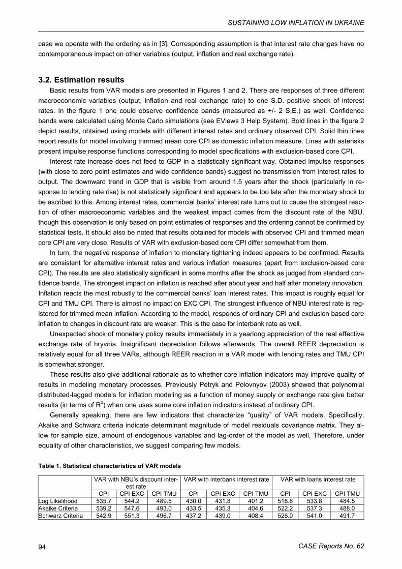
SUSTAINING LOW INFLATION IN UKRAINE
CASE Reports No. 62 94
case we operate with the ordering as in [3]. Corresponding assumption is that interest rate changes have no contemporaneous impact on other variables (output, inflation and real exchange rate).
3.2. Estimation results Basic results from VAR models are presented in Figures 1 and 2. There are responses of three different
macroeconomic variables (output, inflation and real exchange rate) to one S.D. positive shock of interest rates. In the figure 1 one could observe confidence bands (measured as +/- 2 S.E.) as well. Confidence bands were calculated using Monte Carlo simulations (see EViews 3 Help System). Bold lines in the figure 2 depict results, obtained using models with different interest rates and ordinary observed CPI. Solid thin lines report results for model involving trimmed mean core CPI as domestic inflation measure. Lines with asterisks present impulse response functions corresponding to model specifications with exclusion-based core CPI.
Interest rate increase does not feed to GDP in a statistically significant way. Obtained impulse responses (with close to zero point estimates and wide confidence bands) suggest no transmission from interest rates to output. The downward trend in GDP that is visible from around 1.5 years after the shock (particularly in re-sponse to lending rate rise) is not statistically significant and appears to be too late after the monetary shock to be ascribed to this. Among interest rates, commercial banks’ interest rate turns out to cause the strongest reac-tion of other macroeconomic variables and the weakest impact comes from the discount rate of the NBU, though this observation is only based on point estimates of responses and the ordering cannot be confirmed by statistical tests. It should also be noted that results obtained for models with observed CPI and trimmed mean core CPI are very close. Results of VAR with exclusion-based core CPI differ somewhat from them.
In turn, the negative response of inflation to monetary tightening indeed appears to be confirmed. Results are consistent for alternative interest rates and various inflation measures (apart from exclusion-based core CPI). The results are also statistically significant in some months after the shock as judged from standard con-fidence bands. The strongest impact on inflation is reached after about year and half after monetary innovation. Inflation reacts the most robustly to the commercial banks’ loan interest rates. This impact is roughly equal for CPI and TMU CPI. There is almost no impact on EXC CPI. The strongest influence of NBU interest rate is reg-istered for trimmed mean inflation. According to the model, responds of ordinary CPI and exclusion based core inflation to changes in discount rate are weaker. This is the case for interbank rate as well.
Unexpected shock of monetary policy results immediately in a yearlong appreciation of the real effective exchange rate of hryvnia. Insignificant depreciation follows afterwards. The overall REER depreciation is relatively equal for all three VARs, although REER reaction in a VAR model with lending rates and TMU CPI is somewhat stronger.
These results also give additional rationale as to whether core inflation indicators may improve quality of results in modeling monetary processes. Previously Petryk and Polovnyov (2003) showed that polynomial distributed-lagged models for inflation modeling as a function of money supply or exchange rate give better results (in terms of R2) when one uses some core inflation indicators instead of ordinary CPI.
Generally speaking, there are few indicators that characterize “quality” of VAR models. Specifically, Akaike and Schwarz criteria indicate determinant magnitude of model residuals covariance matrix. They al-low for sample size, amount of endogenous variables and lag-order of the model as well. Therefore, under equality of other characteristics, we suggest comparing few models.
Table 1. Statistical characteristics of VAR models
VAR with NBU’s discount inter-est rate
VAR with interbank interest rate VAR with loans interest rate
CPI CPI EXC CPI TMU CPI CPI EXC CPI TMU CPI CPI EXC CPI TMU Log Likelihood 535.7 544.2 489.5 430.0 431.8 401.2 518.8 533.8 484.5 Akaike Criteria 539.2 547.6 493.0 433.5 435.3 404.6 522.2 537.3 488.0 Schwarz Criteria 542.9 551.3 496.7 437.2 439.0 408.4 526.0 541.0 491.7
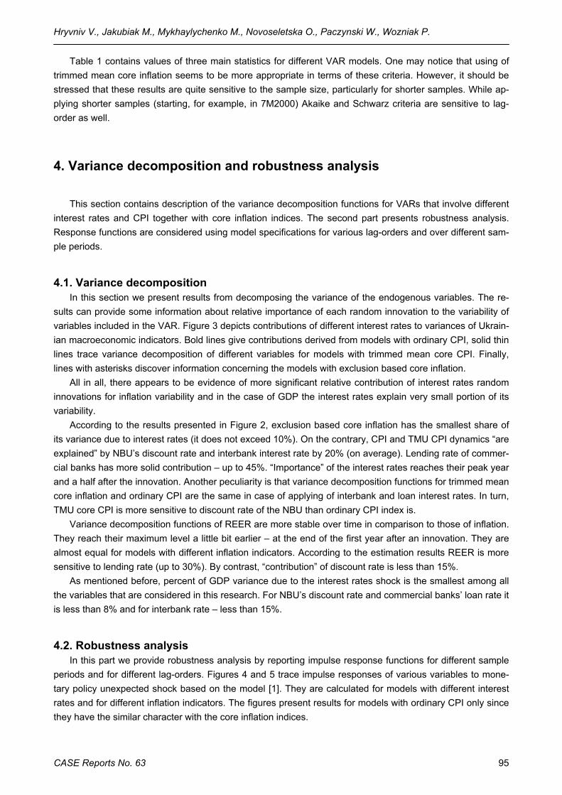
Hryvniv V., Jakubiak M., Mykhaylychenko M., Novoseletska O., Paczynski W., Wozniak P.
CASE Reports No. 63 95
Table 1 contains values of three main statistics for different VAR models. One may notice that using of trimmed mean core inflation seems to be more appropriate in terms of these criteria. However, it should be stressed that these results are quite sensitive to the sample size, particularly for shorter samples. While ap-plying shorter samples (starting, for example, in 7M2000) Akaike and Schwarz criteria are sensitive to lag-order as well.
4. Variance decomposition and robustness analysis
This section contains description of the variance decomposition functions for VARs that involve different interest rates and CPI together with core inflation indices. The second part presents robustness analysis. Response functions are considered using model specifications for various lag-orders and over different sam-ple periods.
4.1. Variance decomposition In this section we present results from decomposing the variance of the endogenous variables. The re-
sults can provide some information about relative importance of each random innovation to the variability of variables included in the VAR. Figure 3 depicts contributions of different interest rates to variances of Ukrain-ian macroeconomic indicators. Bold lines give contributions derived from models with ordinary CPI, solid thin lines trace variance decomposition of different variables for models with trimmed mean core CPI. Finally, lines with asterisks discover information concerning the models with exclusion based core inflation.
All in all, there appears to be evidence of more significant relative contribution of interest rates random innovations for inflation variability and in the case of GDP the interest rates explain very small portion of its variability.
According to the results presented in Figure 2, exclusion based core inflation has the smallest share of its variance due to interest rates (it does not exceed 10%). On the contrary, CPI and TMU CPI dynamics “are explained” by NBU’s discount rate and interbank interest rate by 20% (on average). Lending rate of commer-cial banks has more solid contribution – up to 45%. “Importance” of the interest rates reaches their peak year and a half after the innovation. Another peculiarity is that variance decomposition functions for trimmed mean core inflation and ordinary CPI are the same in case of applying of interbank and loan interest rates. In turn, TMU core CPI is more sensitive to discount rate of the NBU than ordinary CPI index is.
Variance decomposition functions of REER are more stable over time in comparison to those of inflation. They reach their maximum level a little bit earlier – at the end of the first year after an innovation. They are almost equal for models with different inflation indicators. According to the estimation results REER is more sensitive to lending rate (up to 30%). By contrast, “contribution” of discount rate is less than 15%.
As mentioned before, percent of GDP variance due to the interest rates shock is the smallest among all the variables that are considered in this research. For NBU’s discount rate and commercial banks’ loan rate it is less than 8% and for interbank rate – less than 15%.
4.2. Robustness analysis In this part we provide robustness analysis by reporting impulse response functions for different sample
periods and for different lag-orders. Figures 4 and 5 trace impulse responses of various variables to mone-tary policy unexpected shock based on the model [1]. They are calculated for models with different interest rates and for different inflation indicators. The figures present results for models with ordinary CPI only since they have the similar character with the core inflation indices.
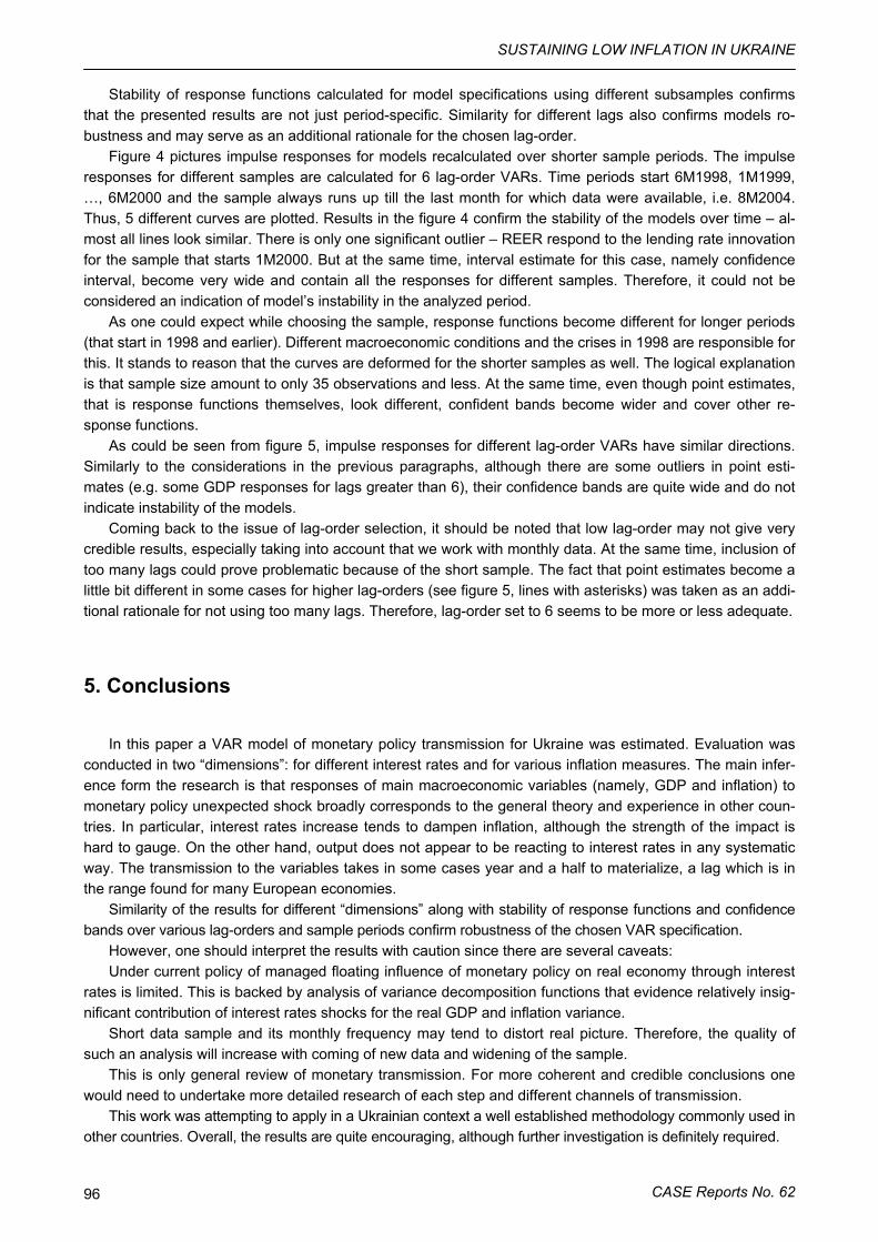
SUSTAINING LOW INFLATION IN UKRAINE
CASE Reports No. 62 96
Stability of response functions calculated for model specifications using different subsamples confirms that the presented results are not just period-specific. Similarity for different lags also confirms models ro-bustness and may serve as an additional rationale for the chosen lag-order.
Figure 4 pictures impulse responses for models recalculated over shorter sample periods. The impulse responses for different samples are calculated for 6 lag-order VARs. Time periods start 6M1998, 1M1999, …, 6M2000 and the sample always runs up till the last month for which data were available, i.e. 8M2004. Thus, 5 different curves are plotted. Results in the figure 4 confirm the stability of the models over time – al-most all lines look similar. There is only one significant outlier – REER respond to the lending rate innovation for the sample that starts 1M2000. But at the same time, interval estimate for this case, namely confidence interval, become very wide and contain all the responses for different samples. Therefore, it could not be considered an indication of model’s instability in the analyzed period.
As one could expect while choosing the sample, response functions become different for longer periods (that start in 1998 and earlier). Different macroeconomic conditions and the crises in 1998 are responsible for this. It stands to reason that the curves are deformed for the shorter samples as well. The logical explanation is that sample size amount to only 35 observations and less. At the same time, even though point estimates, that is response functions themselves, look different, confident bands become wider and cover other re-sponse functions.
As could be seen from figure 5, impulse responses for different lag-order VARs have similar directions. Similarly to the considerations in the previous paragraphs, although there are some outliers in point esti-mates (e.g. some GDP responses for lags greater than 6), their confidence bands are quite wide and do not indicate instability of the models.
Coming back to the issue of lag-order selection, it should be noted that low lag-order may not give very credible results, especially taking into account that we work with monthly data. At the same time, inclusion of too many lags could prove problematic because of the short sample. The fact that point estimates become a little bit different in some cases for higher lag-orders (see figure 5, lines with asterisks) was taken as an addi-tional rationale for not using too many lags. Therefore, lag-order set to 6 seems to be more or less adequate.
5. Conclusions
In this paper a VAR model of monetary policy transmission for Ukraine was estimated. Evaluation was conducted in two “dimensions”: for different interest rates and for various inflation measures. The main infer-ence form the research is that responses of main macroeconomic variables (namely, GDP and inflation) to monetary policy unexpected shock broadly corresponds to the general theory and experience in other coun-tries. In particular, interest rates increase tends to dampen inflation, although the strength of the impact is hard to gauge. On the other hand, output does not appear to be reacting to interest rates in any systematic way. The transmission to the variables takes in some cases year and a half to materialize, a lag which is in the range found for many European economies.
Similarity of the results for different “dimensions” along with stability of response functions and confidence bands over various lag-orders and sample periods confirm robustness of the chosen VAR specification.
However, one should interpret the results with caution since there are several caveats: Under current policy of managed floating influence of monetary policy on real economy through interest
rates is limited. This is backed by analysis of variance decomposition functions that evidence relatively insig-nificant contribution of interest rates shocks for the real GDP and inflation variance.
Short data sample and its monthly frequency may tend to distort real picture. Therefore, the quality of such an analysis will increase with coming of new data and widening of the sample.
This is only general review of monetary transmission. For more coherent and credible conclusions one would need to undertake more detailed research of each step and different channels of transmission.
This work was attempting to apply in a Ukrainian context a well established methodology commonly used in other countries. Overall, the results are quite encouraging, although further investigation is definitely required.
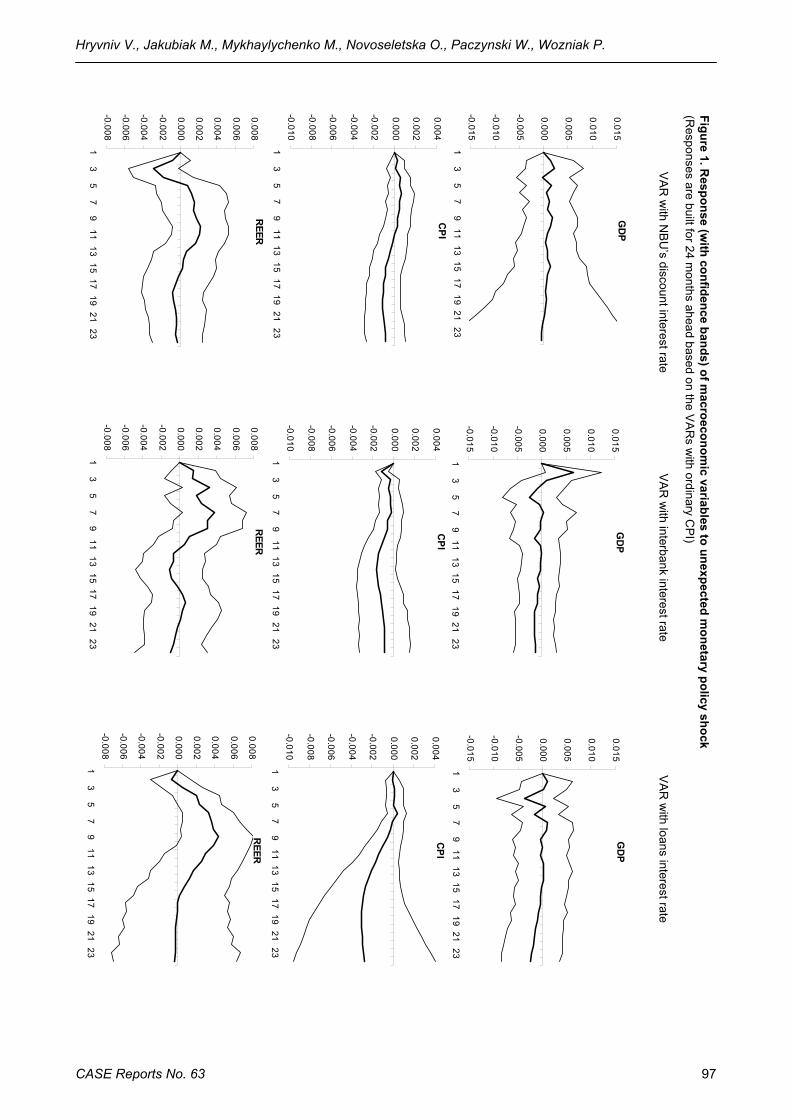
Hryvniv V., Jakubiak M., Mykhaylychenko M., Novoseletska O., Paczynski W., Wozniak P.
CASE Reports No. 63 97
GD
P
-0.015
-0.010
-0.005
0.000
0.005
0.010
0.015
13
57
911
1315
1719
2123
CPI
-0.010
-0.008
-0.006
-0.004
-0.002
0.000
0.002
0.004
13
57
911
1315
1719
2123
REER
-0.008
-0.006
-0.004
-0.002
0.000
0.002
0.004
0.006
0.008
13
57
911
1315
1719
2123
GD
P
-0.015
-0.010
-0.005
0.000
0.005
0.010
0.015
13
57
911
1315
1719
2123
CPI
-0.010
-0.008
-0.006
-0.004
-0.002
0.000
0.002
0.004
13
57
911
1315
1719
2123
REER
-0.008
-0.006
-0.004
-0.002
0.000
0.002
0.004
0.006
0.008
13
57
911
1315
1719
2123
GD
P
-0.015
-0.010
-0.005
0.000
0.005
0.010
0.015
13
57
911
1315
1719
2123
CPI
-0.010
-0.008
-0.006
-0.004
-0.002
0.000
0.002
0.004
13
57
911
1315
1719
2123
REER
-0.008
-0.006
-0.004
-0.002
0.000
0.002
0.004
0.006
0.008
13
57
911
1315
1719
2123
Figure 1. Response (w
ith confidence bands) of macroeconom
ic variables to unexpected monetary policy shock
(Responses are built for 24 m
onths ahead based on the VA
Rs w
ith ordinary CP
I)
V
AR
with N
BU
’s discount interest rate V
AR
with interbank interest rate
VA
R w
ith loans interest rate
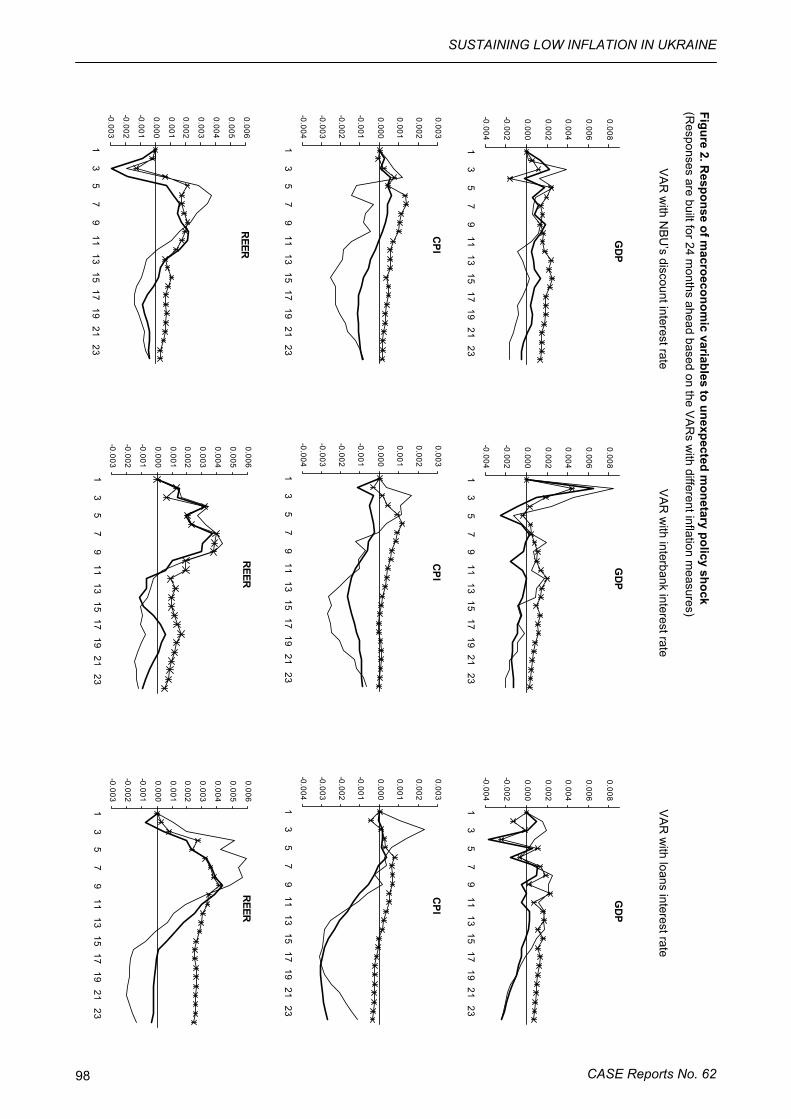
SUSTAINING LOW INFLATION IN UKRAINE
CASE Reports No. 62 98
GDP
-0.004
-0.002
0.000
0.002
0.004
0.006
0.008
13
57
911
1315
1719
2123
CPI
-0.004
-0.003
-0.002
-0.001
0.000
0.001
0.002
0.003
13
57
911
1315
1719
2123
REER
-0.003
-0.002
-0.001
0.000
0.001
0.002
0.003
0.004
0.005
0.006
13
57
911
1315
1719
2123
GDP
-0.004
-0.002
0.000
0.002
0.004
0.006
0.008
13
57
911
1315
1719
2123
CPI
-0.004
-0.003
-0.002
-0.001
0.000
0.001
0.002
0.003
13
57
911
1315
1719
2123
REER
-0.003
-0.002
-0.001
0.000
0.001
0.002
0.003
0.004
0.005
0.006
13
57
911
1315
1719
2123
GDP
-0.004
-0.002
0.000
0.002
0.004
0.006
0.008
13
57
911
1315
1719
2123
CPI
-0.004
-0.003
-0.002
-0.001
0.000
0.001
0.002
0.003
13
57
911
1315
1719
2123
REER
-0.003
-0.002
-0.001
0.000
0.001
0.002
0.003
0.004
0.005
0.006
13
57
911
1315
1719
2123
Figure 2. Response of m
acroeconomic variables to unexpected m
onetary policy shock (R
esponses are built for 24 months ahead based on the V
AR
s with different inflation m
easures)
V
AR
with N
BU
’s discount interest rate V
AR
with interbank interest rate
VA
R w
ith loans interest rate
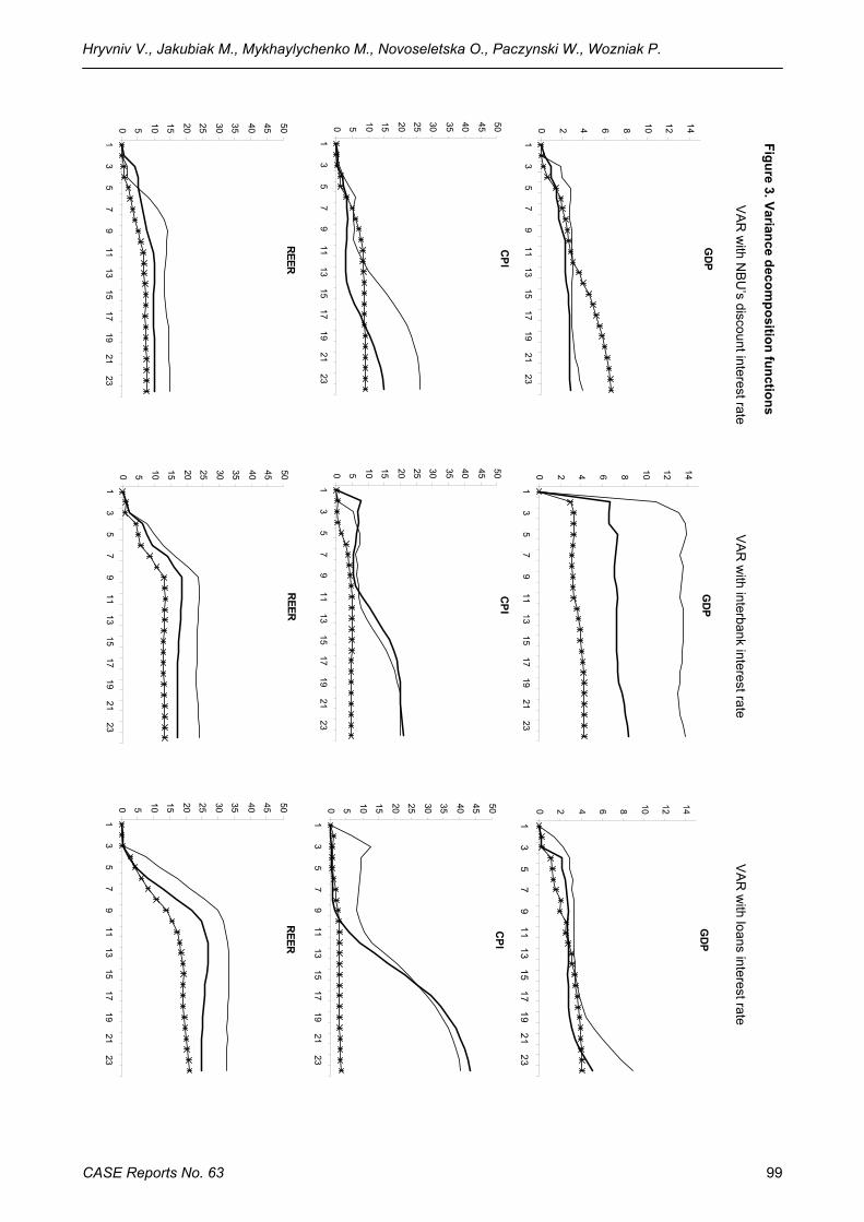
Hryvniv V., Jakubiak M., Mykhaylychenko M., Novoseletska O., Paczynski W., Wozniak P.
CASE Reports No. 63 99
GD
P
0 2 4 6 8 10 12 14
13
57
911
1315
1719
2123
CPI
0 5 10 15 20 25 30 35 40 45 50
13
57
911
1315
1719
2123
REER
0 5 10 15 20 25 30 35 40 45 50
13
57
911
1315
1719
2123
GD
P
0 2 4 6 8 10 12 14
13
57
911
1315
1719
2123
CPI
0 5 10 15 20 25 30 35 40 45 50
13
57
911
1315
1719
2123
REER
0 5 10 15 20 25 30 35 40 45 50
13
57
911
1315
1719
2123
GD
P
0 2 4 6 8 10 12 14
13
57
911
1315
1719
2123
CPI
0 5 10 15 20 25 30 35 40 45 50
13
57
911
1315
1719
2123
REER
0 5 10 15 20 25 30 35 40 45 50
13
57
911
1315
1719
2123
Figure 3. Variance decomposition functions
V
AR
with N
BU
’s discount interest rate V
AR
with interbank interest rate
VA
R w
ith loans interest rate
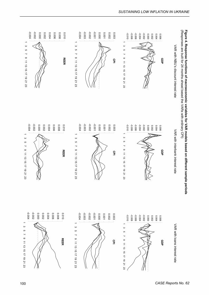
SUSTAINING LOW INFLATION IN UKRAINE
CASE Reports No. 62 100
GDP
-0.010
-0.008
-0.006
-0.004
-0.002
0.000
0.002
0.004
0.006
13
57
911
1315
1719
2123
CPI
-0.004
-0.003
-0.002
-0.001
0.000
0.001
0.002
0.003
13
57
911
1315
1719
2123
REER
-0.004
-0.002
0.000
0.002
0.004
0.006
0.008
0.010
13
57
911
1315
1719
2123
GDP
-0.010
-0.008
-0.006
-0.004
-0.002
0.000
0.002
0.004
0.006
13
57
911
1315
1719
2123
CPI
-0.004
-0.003
-0.002
-0.001
0.000
0.001
0.002
0.003
13
57
911
1315
1719
2123
REER
-0.004
-0.002
0.000
0.002
0.004
0.006
0.008
0.010
13
57
911
1315
1719
2123
GDP
-0.010
-0.008
-0.006
-0.004
-0.002
0.000
0.002
0.004
0.006
13
57
911
1315
1719
2123
CPI
-0.004
-0.003
-0.002
-0.001
0.000
0.001
0.002
0.003
13
57
911
1315
1719
2123
REER
-0.004
-0.002
0.000
0.002
0.004
0.006
0.008
0.010
13
57
911
1315
1719
2123
Figure 4. Response functions of m
acroeconomic variables for VA
R m
odels based on different sample periods
(Responses are built for 24 m
onths ahead based the VA
Rs w
ith ordinary CP
I)
V
AR
with N
BU
’s discount interest rate V
AR
with interbank interest rate
VA
R w
ith loans interest rate
Hryvniv V., Jakubiak M., Mykhaylychenko M., Novoseletska O., Paczynski W., Wozniak P.
CASE Reports No. 63 101
References
Adamyk, Bohdan, Roman Tyrkalo (1999) Monetary policy transmission and its meaning to the effective-ness of NBU activity, Herald of NBU, No.7, рp. 6-11.
Bilan, Olena (2002) Investigating the Liquidity Effect in the Ukrainian Interbank Market, National Univer-sity of Kyiv-Mohyla Academy, MA thesis.
Bolgarin, Igor, Lavan Mahadeva, and Gabriel Sterne. (2000), Some methodological aspects of building and exploiting model of monetary transmission mechanism in Ukraine. Visnyk NBU #11 (November): 4-6 (Деякі методологічні аспекти побудови та використання моделі механізму монетарної трансмісії в Україні, Вісник НБУ, №11, 2000).
Doroshenko, Ihor (2001) Monetary policy of economic growth in the transitional economy. Shevchenko National University, Kyiv, PhD dissertation. (Грошово-кредитна політика економічного зростання у трансформаційній економіці).
Kowalski, Przemysław, Wojciech Paczyński & Łukasz Rawdanowicz (2003) Exchange Rate Regimes and the Real Sector: a Sectoral Analysis of CEE Countries’, Post-Communist Economies, Vol. 15, No. 3.
Lukyanenko, Iryna and Yriy Gorodnichenko (2002) Modern Econometrics Models in Finances, Study Guide.
Mishkin, Frederic S. (1996) The Channels of Monetary Transmission: Lessons for Monetary. Policy, NBER Working Paper 5464. Novoseletska, O., Myhaylychenko, M. (2004) Ukrainian Money Market (Mechanisms of Monetary Policy
Influence on the Economy), CASE-Ukraine, Kyiv, October, unpublished mimeo. Novoseletska, O. (2005) Ukrainian Money Market. In: Jakubiak (ed.) Sustaining Low Inflation in Ukraine.
CASE Report No. 63. Paczynski, W. (2005) Monetary Transmission in Europe: Lessons for Ukraine In: Jakubiak (ed.) Sustain-
ing Low Inflation in Ukraine. CASE Report No. 63. Peersman, Gert and Frank Smats (2001) The Monetary Transmission Mechanism in the Euro Area:
More Evidence from VAR Analysis, ECB Working No. 91. Petryk and Polovnyov (2002) Core inflation: concept and some methods of calculation, Visnyk NBY, De-
cember 2002, pp.47-48. Przystupa, Jan (2002) The exchange rate in the monetary transmission mechanism, NBP, November. Shevchuk, Viktor (2001) The effect of monetary policy on industrial production, inflation and real ex-
change rate in Ukraine during 1994-2000, Herald of NBU, #1, January. Woźniak, P., Mykhaylychenko, M. (2005) Analysis of Core Inflation Indicators in Ukraine. In: Jakubiak
(ed.) Sustaining Low Inflation in Ukraine. CASE Report No. 63. Zaderey, Natalia (2003) Monetary Transmission in Ukraine: is there a Broad Credit Channel, National
University of “Kyiv-Mohyla Academy”, MA thesis. Zivot, Eric (2000) Notes on Structural VAR Modeling, University of Washington, Department of Econom-
ics, Lecture Notes.