1

Cascaded Incremental Nonlinear Dynamic InversionControl for MAV Disturbance Rejection

Ewoud J.J. Smeur, Guido C.H.E. de Croon and Qiping Chu

Abstract—Micro Aerial Vehicles (MAVs) are limited in theiroperation outdoors near obstacles by their ability to withstandwind gusts. Currently widespread position control methods suchas Proportional Integral Derivative control do not perform wellunder the influence of gusts. Incremental Nonlinear DynamicInversion (INDI) is a sensor-based control technique that cancontrol nonlinear systems subject to disturbances. It was devel-oped for the attitude control of manned aircraft or MAVs. Inthis paper we generalize this method to the outer loop control ofMAVs under severe gust loads. Significant improvements over atraditional Proportional Integral Derivative (PID) controller aredemonstrated in an experiment where the quadrotor flies in andout of a windtunnel exhaust at 10 m/s. The control method doesnot rely on frequent position updates, as is demonstrated in anoutside experiment using a standard GPS module. Finally, weinvestigate the effect of using a linearization to calculate thrustvector increments, compared to a nonlinear calculation. Themethod requires little modeling and is computationally efficient.

Index Terms—Quadrocopter, incremental control, INDI, dis-turbance rejection, wind gusts.

I. INTRODUCTION

M ICRO Aerial Vehicles (MAV) have the potential toperform many useful tasks, such as search and rescue

[1], package delivery [2], aerial imaging [3], etc. In many ofthese applications, usage of autonomous MAVs can potentiallyresult in significant cost reduction as compared to currentpractice. But in order to perform these tasks in an outdoorenvironment, the vehicles need to be able to control theirposition under the influence of wind gusts. This is especiallytrue when flying close to obstacles, as a position error due toa wind gust might result in a collision.

Outdoor MAV missions can encounter significant gusts dueto atmospheric turbulence [4]. Moreover, Orr et al. [5] showedthat even a uniform wind can create a very non-uniform windfield in an urban environment. Computational fluid dynamicscalculations showed that with a free stream velocity of 4.6 m/s,flow velocities ranging from 0 to 7.6 m/s are found aroundbuildings. An MAV flying amidst these buildings can beexpected to be subject to up to 7.6 m/s gusts. If such an MAVwere to enter a building through an open window in case of asearch and rescue mission, it would also experience a suddenchange in wind speed. This scenario is especially challengingdue to the confined space of a typical room. And even indoors,an MAV can be subject to aerodynamic disturbances, forinstance caused by its own propeller backwash near walls [6].

The authors are with the Department of Aerospace Engineering,Delft University of Technology, 2629HS Delft, The Netherlands e-mail:e.j.j.smeur@tudelft.nl.

Clearly, a controller that is able to counteract wind gustdisturbances would be of great value. Currently widespreadposition control methods such as Proportional Integral Deriva-tive control (PID), which are used even for aggressive control[7], do not perform well under the influence of gusts. PIDgust rejection properties scale with magnitude of the gains,which is often limited by the GPS update frequency in outdoorscenarios. Moreover, the integrator term is generally slow incompensating persistent wind disturbances.

To cope with wind gusts, a solution could be to use onboardPitot tubes to measure the relative velocity of the MAVwith respect to the wind. The difference with the groundspeed measured by a GPS module can provide an estimateof the local wind [8]. As disturbances may come from alldirections, a minimum of six Pitot tubes would be necessary(two for each axis, as a Pitot tube can not measure negativeairspeed). Alternatively, Mohamed et al. [9] used multiplemulti-probe sensors to obtain flow pitch angle and velocity.Adding such an amount of extra sensors will increase thesystem complexity and cost. Furthermore, airspeed sensors aretypically not reliable at low airspeeds.

Instead of using sensors, one could use a model of the MAVto estimate the wind velocity [10]. Waslander and Wang [11]used an extensive aerodynamic model to estimate wind veloc-ities, with good results in simulation. The downside of thisapproach is that it requires a lot of parameters, which mighteven require windtunnel tests as is done by Schiano et al. [12]and Tomic et al. [13]. If the model does not represent realitywell enough due to modeling errors or airframe changes, thegust disturbance rejection performance will degrade.

In this paper, we introduce a gust resistant controller throughgeneralization of Incremental Nonlinear Dynamic Inversion(INDI) to the outer loop control. The idea is that bothdisturbances as well as control forces are measured by theaccelerometer. This means that a desired acceleration can beachieved by incrementing the previous control input based onthe difference between desired and measured acceleration. Weshow how to deal with filtering of noisy acceleration measure-ments, and how this integrates with the INDI attitude controllerwe developed previously [14]. We will also demonstrate thatthe disturbance rejection capabilities of the INDI inner loopextend to the outer loop control.

The controller is implemented on a Parrot Bebop quadrotorrunning the Paparazzi open source autopilot software1 [15],[16]. Windtunnel experiments show that the quadrotor can

1We have incorporated the INDI control method in Paparazzi, allowingothers to easily experiment with it as well.

arX

iv:1

701.

0725

4v1

[cs

.RO

] 2

5 Ja

n 20

17

2

Fig. 1. The quadrotor in front of the windtunnel during one of theexperiments.

enter and leave the 10 m/s windtunnel flow with only 20cm maximum position deviation on average. A controller thatuses a gain on the integrated error instead of the incrementalcontroller, suffered 146 cm maximum position deviation uponentering and leaving the windtunnel on average. A picture ofthe experiment is shown in Figure 1.

This paper is an extension to the work presented at theIntelligent Robots and Systems conference [17]. Differencesinclude: (1) the use of a large open jet windtunnel as amore accurate and more powerful disturbance than the fanused previously. (2) Incorporation of the propeller thrust curveto calculate the total thrust of the drone. (3) An outdoorsexperiment based on GPS positioning, to demonstrate theperformance in a realistic scenario. (4) The addition of anonlinear method to calculate thrust vector increments.

A. Related Work

Hoffmann et al. [18] developed an altitude controller thatutilizes the vertical acceleration measurement. However, theyfed the acceleration back, multiplied with a gain, withoututilizing the physical relation between thrust and accelera-tion. In a different paper, they state that their PID positioncontrol implementation has little ability to reject disturbancesfrom wind and translational velocity effects [19]. A verticalcontroller using the INDI principle was developed for atraditional helicopter in simulation by Simplicio et al. [20].Only very limited sensor noise was taken into account, whichdid not require any filtering. Also, in both of these papers,by separating the vertical axis from the lateral axes, couplingcan be expected. We show that by inverting the controleffectiveness for all axes, accelerations in each of these axescan be controlled.

Wang et al.[21] applied an acceleration feedback dynamicinversion approach to all axes of a quadrotor, and demon-strated accurate trajectory tracking capabilities. They men-tioned robustness against disturbances, but did not analyzeor demonstrate the controller response against disturbances.

Also, the effects of accelerometer noise or filtering are notdiscussed. Additional differences with the work presented hereare that we do not have a need for a reference model orcommand filtering, and that their approach is not incremental.This means that if a certain control input does not completelyresolve a measured acceleration error (due to input modelingerrors or uncertainties), the error will persist. In an incrementalscheme the input can be incremented again to resolve angularacceleration errors.

II. INCREMENTAL NONLINEAR DYNAMIC INVERSION FORATTITUDE CONTROL

An extended analysis of INDI for attitude control of MAVsis provided in previous work [14]. For completeness, anoverview of the developed attitude controller, along withsome new additions, is presented in this section. Consider thequadrotor shown in Figure 2. The distance from the center ofgravity to each of the rotors along the X axis is given by land along the Y axis by b.

l

Z

X

Y

b

M2

M3

M4

M1

Fig. 2. The Bebop Quadcopter used in the experiments with body axisdefinitions.

We define that Ω is the angular rate vector of the vehicleand the angular rates of the propellers around the body Z axisare described with the vector ω. We also define that T is thethrust provided by all four rotors. Consider Eq. 1, which givesan expression for the angular acceleration and the thrust:[

ΩT

]= F (Ω,v) +G(ω, ω) (1)

Here, F (Ω,v) is the function that describes the vehiclemoments as a function of the angular rates and velocity.G(ω, ω) is the function that maps the input and the derivativeof the input to the angular acceleration and thrust. Note that thethrust force only depends on the rotational rate of the rotors,and so, the fourth row of the F (Ω,v) matrix is zero. Now wecan apply a first order Taylor expansion:[

ΩT

]= F (Ω0,v0) +G(ω0, ω0)

+ ∂∂Ω (F (Ω,v0))|Ω=Ω0

(Ω−Ω0)+ ∂∂v (F (Ω0,v))|v=v0

(v − v0)+ ∂∂ω (G(ω, ω0))|ω=ω0

(ω − ω0)+ ∂∂ω (G(ω0, ω))|ω=ω0(ω − ω0)

(2)

First it can be recognized that the first two terms givethe current angular acceleration and thrust: F (Ω0,v0) +

3

G(ω0, ω0) = [ΩT

0 T0]T . Furthermore we assume thatthe moments due to changes in the function F (Ω,v) aresmall compared to the input moments and can be neglected.Finally, we assume that over the operational domain, the partialderivatives of G(ω, ω) do not change. Therefore, we canapproximate them by the static matrices G1 and G2. Thesecontrol effectiveness matrices are (4×4), because they containthe effectiveness of each of the four rotors on each of the axesroll, pitch, yaw and thrust.

[Ω− Ω0

T − T0

]= G1(ω − ω0) + TsG2(ω − ω0) (3)

Here, the sample time Ts is factored out of G2 to sim-plify future calculations. The angular acceleration Ω0 can bedetermined, by deriving it from the gyroscope using finitedifference. This signal is often very noisy, because the rotatingpropellers lead to vibrations in the airframe. From Bacon etal.[22], we adopt the use of a second order filter, given by:

H(s) =ω2n

s2 + 2ζωns+ ω2n

(4)

This filter also introduces a delay. To be able to apply theTaylor expansion, terms with index 0 should be from the samemoment in time. This is why all these terms should be filteredwith the same filter, such that they are equally delayed. Theseterms are given the subscript f in Eq. 5.

[Ω− Ωf

T − Tf

]= G1(ω − ωf ) + TsG2(ω − ωf ) (5)

By approximating ω and ωf with finite difference, using thelag operator L as ω = (ω(k)−ω(k−1))/Ts = (ω−Lω)/Tsand rearranging the terms, we arrive at:

[Ω− Ωf

T − Tf

]= (G1 +G2)(ω − ωf )−G2L(ω − ωf ) (6)

This equation can now be inverted, to yield Eq. 7.

ωc = ωf+ (G1 +G2)−1

·([νΩ − Ωf

T

]+G2L(ωc − ωf )

)(7)

Here, νΩ is the virtual control, which is the desired angularacceleration that has now become an input. In the next sectionwe will show that the thrust increment T −Tf is calculated inthe outer loop, and is therefore denoted by T . The subscriptc is added to ω to indicate that this is the command sent tothe motors.

The control diagram is shown in Figure 3. The input tothis diagram is the angular acceleration virtual control andthe output is the angular acceleration of the vehicle. Theangular acceleration error, and the thrust increment go into theinversion of the control effectiveness. The increment in motorcommand is added to the feedback from the motors, which isfiltered with the same filter as the angular acceleration. Theactuator dynamics are denoted by A(z).

A. Attitude Control

The control law of Eq. 7 describes how to track angularaccelerations. A PD controller can be used to provide theangular acceleration that will steer the vehicle towards adesired attitude, as is shown in Figure 4.

In this figure we assume small angles, in order to allowsimple integration of the rates to obtain the attitude. In reality,we use a quaternion attitude representation, with the appro-priate feedback, as described by Fresk and Nikolakopoulos[23]. That means that the proportional gain for the quaternionrepresentation has to be twice as large as Kη from Figure 4,since the quaternion derivative is defined as:

q =1

2q ⊗

[0Ω

](8)

where ⊗ denotes the Hamilton product. In previous research[14] we have shown that if the assumptions, mentioned in thederivation of the controller, hold true, the transfer functionfrom νΩ to Ω is simply the actuator dynamics A(z). Whenthe actuator dynamics can be modeled, for instance by firstorder dynamics, the P and D gains can be determined basedon the desired poles and zeros of the system. For the Bebop,the actuator dynamics are modeled with first order dynamicsas shown in Eq. 9, with α = 0.1.

A(z) =α

z − (1− α)(9)

Then the transfer function of the closed loop system fromFigure 4 is as follows:

TFηref→η =KΩKηαT

2s

z3−(3−α)z2+(3−2α+KΩαTs)z+(−1+α−KΩαTs+KΩKηαTs)

(10)

With KΩ = 28 and Kη = 10.7, there is one pole at 0.964and two complex poles at 0.968±0.0463. All poles are withinthe unit circle and the response is fast with little overshoot.

0 0.05 0.1 0.15 0.2 0.25 0.3

Time [s]

-0.05

0

0.05

0.1

0.15

0.2

0.25

0.3

0.35

0.4

0.45

φ[rad

]

σ

µ

design

Fig. 5. Comparison of the designed response and the actual response of theattitude of the quadrotor. The black line is the average, and the gray area onestandard deviation of 25 repetitions.

4

+−

+ (G1 +G2)−1 +

H(z)

A(z)

1z

MAV

Tszz−1

1z

G21z

H(z)z−1Tsz

νΩ Ωerrω ωc

ωfω

T

Ω0ΩfΩf

Ω

Fig. 3. The inner INDI control structure.

+− Kη

+− KΩ A(z) Tsz

z−1Tszz−1

ηref Ωref Ω Ω η

INDI

Fig. 4. The design of the attitude controller for small angles, based on the closed loop response of the INDI controller.

An interesting question is how close the theoretically de-signed response of the attitude matches the actual attituderesponse of the quadrotor. To test this, we subject both theabove transfer function and the real quadrotor to a step input.For the real quadrotor, the step input is repeated 25 times,and the mean and standard deviation are shown in Figure5. The response of the above transfer function is shown inthe same figure in red. The difference between the designedresponse and the actual response is rather small: the error as apercentage of the step magnitude is maximum 6.4 % at 0.14 s.This means that this is a valid way of designing the P and Dgains, based solely on the first order actuator dynamics model.

III. INCREMENTAL NONLINEAR DYNAMIC INVERSIONAPPLIED TO LINEAR ACCELERATIONS

Now that we have a controller that controls the attitude ofthe quadrotor, we can derive an incremental controller for thelinear acceleration of the vehicle. Two reference frames willbe used throughout this derivation; the body frame, as depictedin Figure 2, and the North East Down (NED) frame. Vectorsin the body frame have a subscript B and vectors in the NEDframe have subscript N . The subscripts will only be used toavoid confusion, the position ξ and velocity ξ of the quadrotorwill always be in the NED frame.

The position dynamics are given by Newton’s second lawof motion:

ξ = g +1

mF (ξ,w) +

1

mTN (η, T ) (11)

Where ξ is the acceleration of the MAV, g is the gravityvector and m is the mass. F is the aerodynamic force workingon the airframe as a function of the velocity ξ of the MAVand the wind vector w. TN is the thrust vector in the NED

frame as a function of the attitude η = [φ, θ, ψ]T and the totalthrust produced by the four rotors T .

The thrust vector in the NED frame can be obtainedby taking the thrust vector in the body frame, given byTB = [0, 0, T ]T , and rotating it using the rotation matrixMNB(η). Since the thrust vector in the body frame only hasa Z component, only the last column of the rotation matrixis relevant. The thrust vector in the NED frame is thereforegiven by:

TN (η, T ) = MNB(η)TB =

(sφsψ + cφcψsθ)T(cφsψsθ − cψsφ)T

(cφcθ)T

(12)

where the sine and cosine functions are abbreviated by theletters s and c respectively. Now we can apply a first orderTaylor expansion to Eq. 11, resulting in Eq. 13:

ξ = g + 1mF (ξ0,w0) + 1

mTN (η0, T0)

+ ∂∂ξ

1mF (ξ,w0)|ξ=ξ0

(ξ − ξ0)

+ ∂∂w

1mF (ξ0,w)|w=w0(w −w0)

+ ∂∂φ

1mTN (η, T0)|φ=φ0(φ− φ0)

+ ∂∂θ

1mTN (η, T0)|θ=θ0(θ − θ0)

+ ∂∂T

1mTN (η0, T )|T=T0

(T − T0)

(13)

The first term can be simplified to the acceleration at theprevious timestep: g + 1

mF (ξ0) + 1mTN (η0, T0) = ξ0. This

acceleration can be obtained by rotating the specific forcemeasured by the accelerometer in the body axes to the NEDframe and adding the gravity vector. For the next two terms,the partial derivative of F with respect to ξ and w, we donot have a good estimate. For simplicity of the approach, wechoose not to employ a model of the aerodynamic drag of theairframe. Moreover, it is very difficult, if not impossible, to

5

predict how the wind is going to change. Therefore, the bestguess for these terms is zero. Note that this does not meanthat all aerodynamic forces are neglected. These forces willbe measured with ξ0. Combining this with Eq. 12 and 13 weend up with:

ξ = ξ0 +1

mG(η0, T0)(u− u0) (14)

where u = [φ θ T ]T and

G(η, T ) = (cφsψ − sφcψsθ)T (cφcψcθ)T sφsψ + cφcψsθ(−sφsψsθ − cψcφ)T (cφsψcθ)T cφsψsθ − cψsφ

−cθsφT −sθcφT cφcθ

(15)

The measured accelerations, necessary to obtain ξ0, aretypically noisy due to vibrations in the airframe introducedby the spinning propellers. Therefore, the accelerations needto be filtered. Like in the previous section, the delay of thefilter needs to be accounted for. This is why also here, all termswith subscript 0 will be filtered with the same filter, and begiven a subscript f . Then, if we invert Eq. 14, we obtain theINDI control law for linear accelerations:

uc = uf +mG−1(η0, T0)(ν ξ − ξf ) (16)

We have replaced ξ with the virtual control ν ξ to indicatethat this is now an input to the equation (the desired acceler-ation), and we added the subscript c to u to indicate that thisis the command that will be sent to the inner loop controller.We also define the control increment to be u = uc − uf , soclearly Eq. 16 is an incremental control law.

Suppose we filter the inner loop with filter f1, and the outerloop with filter f2. The thrust increment required by the innerloop is then T − Tf1

. The thrust increment calculated by theouter loop is T−Tf2

. We can only pass on the thrust incrementfrom the outer to the inner loop if these filters are equal. Thatis why for both loops, we use the filter described by Eq. 4,with the same parameters.

IV. IMPLEMENTATION

The implementation of the control law given by Eq. 16 isshown in Figure 6. The input of this diagram is the virtualcontrol, and the output is the acceleration in NED frame.The acceleration in NED frame can be obtained from theaccelerometer measurements with a simple rotation matrix andthe addition of the gravity vector. Increments in roll, pitch andthrust are obtained from the error in acceleration multipliedwith the inverse of the control effectiveness matrix. The rolland pitch increments are added to the filtered measurement ofroll and pitch. Note how the increment in thrust command Tgoes directly into the inner loop.

A. Position Control

In the previous sections, we have shown how the linearacceleration can be controlled using an INDI controller. Tocontrol the position of the MAV, an acceleration referenceneeds to be passed to the outer INDI controller that will steerthe MAV towards its target position. This can be done by a

Proportional Derivative (PD) controller, as is shown in Figure7. The gains of this PD controller were manually tuned.

They depend mainly on two things: the update rate of theposition estimate and the speed of the inner loop controller,which is only dependent on the actuator dynamics. This is thecase because all other components are inverted in the inversionstep of the inner and outer loop. Therefore, if these parametersare known in advance, one can come up with an estimate ofthe PD gains, for instance based on a pole/zero analysis.

B. Adaptive Control Effectiveness

In our previous work we used a Least Mean Squaresalgorithm to adapt the control effectiveness matrix of the rotorsonline. Now, with respect to our previous work, we have addeda row to the control effectiveness matrix that predicts a changein thrust based on the actuator inputs. This row of the controleffectiveness matrix can also be adapted online, together withthe rest of the matrix. The LMS algorithm then becomes:

G(k) = G(k − 1)

−µ2

(G(k − 1)

[∆ωf∆ωf

]−[

∆Ωf

∆T

])[∆ωf∆ωf

]Tµ1

(17)Where:

G(k) =[G1(k) G2(k)

](18)

This means that the effectiveness of the motors with respectto the thrust can also be adapted online. This can be importantif the weight of the vehicle changes during flight, for instancewhen dropping a payload. Given a flight with enough excita-tion of the control input and limited disturbances, the controleffectiveness converges to the control effectiveness calculatedoffline.

C. Estimation of the Thrust

Throughout the derivation of the outer loop INDI controller,we made use of the thrust T , for instance in the matrixG(η, T ). One possibility would be to measure the specificforce in the body Z axis with the accelerometer, and use thisas an estimate for the specific thrust ( Tm ). This approach workswell while hovering, but can lead to errors when there are other(aerodynamic) forces in the body Z axis. These forces occurfor instance at high speed steady flight, when the drone has ahigh bank angle.

Therefore, we used static thrust measurements to model thethrust/rotational rate curve of the propellers. The quadrotorwas mounted upside down on a scale to obtain a measurementof the produced thrust. The rotational rate of the propellers wasobtained from the internal rpm measurement. The results areshown in Figure 8. A quadratic function showed a good fitwith the data. This function is used for the thrust estimate inthe calculations of the controller.

Of course, the actual thrust of the propellers may be slightlydifferent in a real flight, due to a different inflow. Furthermore,since the propellers have a quadratic thrust curve, their controleffectiveness changes depending on their current rotationalrate. In this paper, we assume that the control effectiveness

6

+− mG(η0, T0)−1

+

H(z)

Inner loop

1z

MAV

1z

H(z)

ν ξ ξerr [φ

θ

] [φcθc

]

[φfθf

] [φθ

]

T

ξ0

ξf

ξ

Fig. 6. The outer INDI control structure.

+− Kξ

+− Kξ Outer INDI

Tszz−1

Tszz−1

ξref ξref ν ξ ξ ξ ξ

Fig. 7. The PD controller for the position.

40 60 80 100 120 140 160

Propeller rotational speed(Hz)

0

0.5

1

1.5

Thrust

(N)

Fig. 8. Thrust measurements for different rotor speeds along with a secondorder approximation.

of the rotors with respect to the specific force can be approx-imated by a static one. This removes the need to recalculate(G1 + G2)−1 after every time step, enhancing the speed ofthe algorithm.

Errors introduced by these simplifications are expected tohave low impact, because of the incremental nature of thecontroller. If an increment in thrust does not lead to the desiredacceleration, another increment is applied. This way, smallerrors in the control effectiveness are handled naturally.

D. Linearization

In the previous section, we used a first order Taylor expan-sion to derive the INDI control law. However, from Equation12 it can be seen that the force is actually very nonlinear in

terms of roll and pitch. In Equation 15 it can be seen thatsome of the derivatives can even change sign, for instance ∂z

∂φfor different values of φ.

What this means in practice is that if the increments in theinput are large, because suddenly a large lateral accelerationis required, they will result in a different acceleration thanintended. This will be measured by the accelerometer, andsubsequent increments in the inputs will eventually lead to theright acceleration. But it might be more effective to implementa nonlinear method of finding increments in the input that giveexactly the desired increment in the acceleration.

Since we have the nonlinear function of our inputs available,it is possible to do a nonlinear inversion. At the same time,we would like to keep the incremental structure, because wedon’t have an accurate estimate of the aerodynamic forces F .If we refer to Eq. 11, we can subtract the same formula a shorttime instant earlier:

ξ − ξ0 = g − g0 + 1mF (ξ,w)− 1

mF (ξ0,w0)+ 1mTN (η, T )− 1

mTN (η0, T0)(19)

We assume changes in gravity and the aerodynamic forcesare small during this small time instant:

ξ − ξ0 =1

mTN (η, T )− 1

mTN (η0, T0) (20)

If we desire a different acceleration, we now know whatthe increment in the thrust vector should be. We can calculatewhat the current thrust vector is based on the attitude androtational rate of the rotors. This gives an expression for thenew thrust vector:

TN (η, T ) = m(ξ − ξ0) + TN (η0, T0) (21)

How the thrust vector depends on the thrust and attitude isdescribed by Eq. 12. We can do a nonlinear inversion of this

7

equation to obtain expressions for the thrust, roll and pitchcommands:

T = ||TN || (22)

φc = arcsin

(sin(ψ)TNx − cos(ψ)TNy

T

)(23)

θc = arcsin

(cos(ψ)TNx + sin(ψ)TNy

T cosφc

)(24)

This allows us to find a new attitude and thrust that willsatisfy a desired acceleration, without linearizing the inputfunction. At the same time, we have retained the incrementalstructure, as we calculate the new thrust vector based on theprevious one. For the nonlinear case, the same argument holdsregarding the filtering as for the linearized case: if we filterthe acceleration, we should also filter the other signals withsubscript 0. This is shown below:

TN (η, T ) = m(ξ − ξf ) + TN (ηf , Tf ) (25)

E. Filtering

Both the measured accelerations as well as the rates are fil-tered to remove noise. In the derivation of the INDI controller,we showed that these signals should be filtered with the samefilter. This way, the delay in both loops is synchronized andthe thrust increment can go from the outer loop to the innerloop.

Previously, we have shown that the filter choice has an effecton the disturbance rejection [14]. For the attitude loop, theresponse to a disturbance is given by (1−A(z)H(z)z−1). Bytaking a filter with a higher cutoff frequency, and thereforeless delay, disturbances will be rejected faster. On the otherhand, more noise will end up in the control signals. Since theinner and outer INDI loops are connected and need to use thesame filter, this trade-off should be considered for both loopssimultaneously. For the experiment, we chose a filter with aωn = 50 rad/s and ζ = 0.55.

F. Accelerometer Bias

The outer loop INDI controller is somewhat sensitive toaccelerometer biases. Because the accelerometer measurementis fed back to control the acceleration, an offset in the mea-surement will result in an offset in the actual acceleration aswell. This means that the quadrotor will maintain its positionnot at a position with zero error, but at a position where theposition error times the P gain gives a required accelerationequal to minus the acceleration offset.

This problem does not arise in the inner loop, where theangular acceleration is bias free. This is because in calculatingthe derivative of the rates, the bias disappears from the signal.This is not the case for the outer loop, so we need to estimatethe accelerometer bias in order to remove it. As a secondmeasurement we have the velocity and position from GPS oran indoor positioning system. The velocity measurement canbe derived to obtain a bias free acceleration measurement. The

measurement of the velocity only has a low update rate, so thissignal is not really viable for feedback.

However, the acceleration obtained from velocity can beused to determine the accelerometer bias. The accelerometerbias is a signal that is assumed to vary only very slowly. Thisis why we filter both the accelerometer and the accelerationobtained from the velocity measurement with a second orderfilter with a natural frequency of 0.25 rad/s. This removesall noise while keeping the important bias information. Thesignals are both filtered with the same filter such that they havethe same delay. After the filtering, the signals are subtracted tofind the accelerometer bias. This is only a very simple methodof finding the accelerometer bias, it could alternatively be donewith a Kalman filter.

V. WINDTUNNEL EXPERIMENT

The goal of the experiment is to test how well the INDIcontroller can handle gust disturbances. The experiment isperformed indoors, such that there is a controlled environmentin which repeatable experiments can be performed. The sourceof the wind disturbance is the Open Jet Facility of the TUDelft Aerospace department. It has a 2.85 m by 2.85 m crosssection, and is capable of velocities up to 30 m/s. A picture ofthe drone flying in front of the windtunnel is shown in Figure1. Because the windtunnel is not capable of rapidly increasingor decreasing its velocity, the quadrotor has to fly in and outof the windtunnel exhaust to simulate a gust. This is done byletting the quadrotor alternate between two waypoints every14 seconds, one being in the center of the of the windtunnelexhaust, and one being 2 meters west of this point.

The INDI loop basically controls the acceleration of theMAV. From this perspective, it is an addition to a PIDcontroller, where with INDI the integral gain is zero. Thisis why we will compare the performance of INDI with aregular PID controller. The PID controller is manually tunedto give the fastest response possible without oscillation. Boththe INDI as well as the PID outer loop controllers make useof the inner loop INDI controller for attitude control. For thePID controller, the P, I and D gains work directly on theposition and velocity to produce a reference roll, pitch andthrust. In tuning these gains, there is a trade-off to be made.By increasing the integral gain, faster offset compensationcan be obtained. This way the quadrotor can adjust to thedisturbance of the windtunnel faster. However, with a highintegral gain, the quadrotor will also have more overshoot inreference tracking tasks such as sudden position changes. Thistrade-off is non-existent for the INDI controller.

We can do a crude comparison between the Kξ and Kξ

gains of the INDI controller and the P and D gains of thePID controller. Around hover, the virtual control is related tothe change in commanded attitude angle through a divisionby gravity, assuming small angles. Kξ and Kξ then become0.70 (m/s)/m and 0.15 rad/(m/s) respectively. For the PIDcontroller, the corresponding P and D gains are 0.65 (m/s)/mand 0.20 rad/(m/s) respectively. Though these gains are notexactly the same, the goal of this crude comparison is to showthat both controllers have roughly the same gains. Since we

8

will consider disturbance rejection properties, the integral gainwill play the biggest role.

The MAV used for the experiments is the Bebop quadrotorfrom Parrot. Instead of the stock firmware, it is running thePaparazzi open source autopilot system. An infrared motiontracking system called ’Optitrack’ was used to obtain positioninformation. This system can measure the drone’s positionwith millimeter accuracy at a frequency up to 120 Hz. Butbecause we want the experiment to be realistic for outsidescenarios and since most Global Positioning System (GPS)modules can only provide position updates at four Hz, thedata was only sent to the drone at a frequency of four Hz. Thecontrol algorithm, as well as the onboard accelerometer andgyroscope, were running at 512 Hz. In an outdoor scenario,millimeter accuracy might not be achievable with off theshelve GPS modules. But even though the position might beoff in such a case, gusts will still be rejected the same way asin this indoor experiment, as the INDI controller is based onthe accelerometer.

A. Results

First, consider Figure 9. It shows the acceleration in thenorth axis, which is the axis in which the windtunnel isblowing. The acceleration is filtered with a second order filterwith ωn = 20 rad/s and ζ = 0.7. At 113.6 seconds, thequadrotor is commanded to fly into the wind. The momentthe quadrotor flies into the wind stream is clearly visible inthe figure due to the large acceleration spike, deviating fromthe reference acceleration. Due to this acceleration error, theINDI controller will increment the control inputs in order tomake the acceleration track the reference again. About halfa second after the start of the disturbance, the accelerationcoincides with the reference acceleration, effectively havingcounteracted the disturbance. At that point, the quadcopterhas built up a speed and position error in the north axis. Thequadrotor needs a positive acceleration after the disturbanceto bring these errors back to zero.

110 115 120 125 130 135 140

Time [s]

-1.5

-1

-0.5

0

0.5

1

1.5

ξ[m

/s2]

ξ

ξref

Fig. 9. Acceleration in the north direction for the INDI controller.

The same thing happens at 127.5 seconds, when the quadro-tor is commanded to fly out of the wind again. Now thesudden absence of wind results in a disturbance in the oppositedirection. What also can be observed from this figure is that theaccelerometer measures a more high frequency signal whenflying in the wind. This could be due to the airflow containingsome turbulence.

Figure 10 shows the position along the XN axis, for boththe INDI and PID controllers. The Figure shows the averageof seven times the same maneuver, along with one standarddeviation. For INDI, we can observe that a position error of0.2 m occurs upon entering (113.6 seconds) or leaving (127.5seconds) the windtunnel. This position error is counteractedwithin three seconds after it occurred.

Fig. 10. Position in the North direction for the INDI and PID experiment.The line is the average of seven repetitions, and the colored areas indicateone standard deviation.

Compare this with the position for the PID controller in thesame figure. The maximum error is 1.5 m, and it takes longerfor the position error to be counteracted as compared to theINDI controller. One thing to note is that, when the vehicleis flying in the windtunnel (20-28 seconds) and there are nochanging disturbances, there is very little variance betweenflights. This difference may be attributed to the fact thatthe INDI controller is using the accelerometer for feedback.Though the accelerometer measurement is filtered, it is still abit noisy. A filter with more high frequency attenuation couldhave been used, but this would make the disturbance rejectionof the controller slightly slower, because such a filter has moredelay.

A top view of the experiment is shown in figure 11. Fromthis figure the difference in performance becomes apparent.The Figure shows the entire flight, from takeoff until landing.For the PID controller, you can see how it is blown in thenegative XN direction upon takeoff, entering the windtunnel,and how it overshoots in a straight line upon landing, leavingthe windtunnel flow. The INDI controller is able to cope muchbetter with the sudden wind changes during taking off andlanding.

9

-2.5 -2 -1.5 -1 -0.5 0 0.5

YN [m]

-2

-1.5

-1

-0.5

0

0.5

1

1.5X

N[m

]

INDI

PID

Fig. 11. Top view of the experiment for the PID and INDI controllers at 10m/s.

VI. OUTDOOR TAKEOFF WITH WIND

The experiment in the windtunnel is great from a scientificpoint of view, as it allows us to compare different controllerssubject to exactly the same disturbance. On the other hand,since we used an Optitrack system for position estimation,it might not be clear if the controller can provide the sameperformance in an outdoor scenario. That is why we performeda second experiment; outdoors and with a standard off-the-shelve GPS receiver.

One of the situations in which an MAV needs to cope witha sudden wind disturbance, is during takeoff on a windy day.When on the ground, the ground is compensating the dragfrom the wind. But when the drone takes off, the wind forcewill accelerate the drone. Therefore, a control action is neededto counteract the wind and maintain position.

Since the acceleration is measured with the accelerometer,it is expected that the INDI controller will compensate for thewind force very fast. A PID controller that does not use thisinformation, on the other hand, is expected to drift a bit, untilit has gained some error in position and velocity that causes itto steer back. The integrator part will remove the steady stateerror over time.

Like before, we are using the first version of the Bebopquadrotor for this experiment. As opposed to the secondversion of the Bebop, the first version that is used for thisexperiment has a low quality GPS. With the built-in GPS, thedisturbance rejection performance is hard to evaluate, as theposition estimate will move around quite a bit, regardless if thedrone is moving or not. This is why the quadrotor is equippedwith an external Ublox Neo M8N through a USB connection.This GPS module is commercially available, and the secondversion of the Bebop even ships with this module built in.

Like the windtunnel experiment, we will compare the casewith outer loop INDI and without. The PID controller has thesame gains as in the windtunnel experiment, just like the Pand D gains that produce the acceleration reference for theINDI controller are the same.

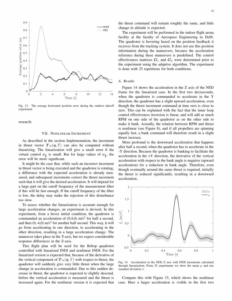
Fig. 12. The horizontal position error during the outdoor takeoff experiment.

A. Results

On the day of the outdoor takeoff experiment an averagewind speed of 5.1 m/s was reported by the Dutch Meteorolog-ical Institute (KNMI). Over the course of one and a half hour,first twelve flights were performed with the PID controller,and then thirteen with the INDI controller. The flights wereperformed one after the other, without breaks. It is assumedthat on average, the wind during the INDI flights was the sameas during the PID flights, even though a fluctuation of the windspeed between flights was observed.

One of the flights with the INDI controller was rejected, asfrom the data it became clear that the state estimation filterhad not converged prior to takeoff. The state estimation errorleads to a bias in the NED acceleration, which in turn leadsto a position offset, as discussed above.

The position error can be seen in Figure 12. The averageposition error is shown in Figure 13.

The position reference was reset to the current position justbefore each flight, so all flights start with a position errorclose to zero. As expected, during the takeoff INDI performsmuch better than the PID controller. It can be seen from Figure13 that the INDI controller produces on average a maximumposition error of 0.24 m as compared to 0.85 m for the PIDcontroller.

Though Figure 13 shows that the average error after sometime is the same for both controllers, it appears from Figure12 that there are some runs for the INDI controller withrelatively large errors. These errors are especially large ifthey are compared to the position error that is the result ofthe takeoff in the wind, which was expected to be the maindisturbance. Closer inspection of some of these datasets showthat when these errors occur, the acceleration measured bythe accelerometer does not correspond with the position andvelocity measured by the GPS. This may indicate that theseerrors are caused by by GPS errors, perhaps upon changingbetween satellites. This could perhaps be solved with a betterstate estimation algorithm, but that is beyond the scope of this

10

0 2 4 6 8 10 12 14

Time [s]

0

0.1

0.2

0.3

0.4

0.5

0.6

0.7

0.8

0.9Average

positionerror[m

]

INDI

PID

Fig. 13. The average horizontal position error during the outdoor takeoffexperiment.

research.

VII. NONLINEAR INCREMENT

As described in the section Implementation, the incrementin thrust vector TN (η, T ) can also be computed withoutlinearizing. The linearization will give a small error if thevirtual control ν ξ is small. But for large values of ν ξ, theerror will be more significant.

It might be the case that, while such an incorrect incrementin thrust vector is being executed and the quadrotor is rotating,a difference with the expected acceleration is already mea-sured, and subsequent increments correct the thrust incrementsuch that it will give the desired acceleration. It will depend fora large part on the cutoff frequency of the measurement filterif this will be fast enough. If the cutoff frequency of the filteris low, the delay may make the rejection of this disturbancetoo slow.

To assess whether the linearization is accurate enough forlarge acceleration changes, an experiment is devised. In thisexperiment, from a hover initial condition, the quadrotor iscommanded an acceleration of (0,4,0) m/s2 for half a second,and then (0,-4,0) m/s2 for another half second. This way, it willgo from accelerating in one direction, to accelerating in theother direction, resulting in a large acceleration change. Themaneuver takes place in the Y-axis, but we expect considerableresponse differences in the Z-axis.

This flight plan will be used for the Bebop quadrotorcontrolled with linearized INDI and nonlinear INDI. For thelinearized version is expected that, because of the derivative ofthe vertical component of TN (η, T ) with respect to thrust, thequadrotor will suddenly give very little thrust when the largechange in acceleration is commanded. Due to this sudden de-crease in thrust, the quadrotor is expected to slightly descend,before the vertical acceleration is measured and the thrust isincreased again. For the nonlinear version it is expected that

the thrust command will remain roughly the same, and littlechange in altitude is expected.

The experiment will be performed in the indoor flight arenafacility at the faculty of Aerospace Engineering in Delft.The quadrotor is hovering based on the position feedback itreceives from the tracking system. It does not use this positioninformation during the maneuvers, because the accelerationreference during these maneuvers is predefined. The controleffectiveness matrices G1 and G2 were determined prior tothe experiment using the adaptive algorithm. The experimentis done with 25 repetitions for both conditions.

A. Results

Figure 14 shows the acceleration in the Z axis of the NEDframe for the linearized case. In the first two deciseconds,when the quadrotor is commanded to accelerate in the Ydirection, the quadrotor has a slight upward acceleration, eventhough the thrust increment command at time zero is close tozero. This can be explained with the fact that the inner loopcontrol effectiveness inversion is linear, and will add as muchRPM on one side of the quadrotor as on the other side tomake it bank. Actually, the relation between RPM and thrustis nonlinear (see Figure 8), and if all propellers are spinningequally fast, a bank command will therefore result in a slightthrust increase.

More profound is the downward acceleration that happensafter half a second, when the quadrotor has to accelerate in the-Y direction. Because the quadrotor is banking to facilitate theacceleration in the +Y direction, the derivative of the verticalacceleration with respect to the bank angle is negative (upwardacceleration) for a reduction in bank angle. Therefore, eventhough eventually around the same thrust is required, initiallythe thrust is reduced significantly, resulting in a downwardacceleration.

0 0.2 0.4 0.6 0.8 1

Time [s]

-0.5

0

0.5

1

1.5

2

ξ z[m

/s2]

σ

µ

Fig. 14. Acceleration in the NED Z axis with INDI increments calculatedthrough linearization. From 25 experiments we show the mean µ and onestandard deviation σ.

Compare this with Figure 15, which shows the nonlinearcase. Here a larger acceleration is visible in the first two

11

deciseconds. This is caused by the fact that the actuator dy-namics are faster than the rotational dynamics. The nonlinearincrement is calculated for the tilted thrust vector, thereforea positive thrust increment is commanded by the outer loopINDI controller. However, the rotational dynamics are slowerthan the thrust dynamics. Therefore, the thrust is increasedalready before the final attitude is attained. This causes thevehicle to accelerate upwards initially.

0 0.2 0.4 0.6 0.8 1

Time [s]

-1

-0.5

0

0.5

1

1.5

ξ z[m

/s2]

σ

µ

Fig. 15. Acceleration in the NED Z axis with INDI increments calculatedthrough nonlinear calculation. From 25 experiments we show the mean µ andone standard deviation σ.

After half a second, when the large acceleration change iscommanded, the response is quite different from the linearcase. Instead of acceleration downward, the vehicle acceleratesupward. This can be explained by recognizing that the quadro-tor will need more or less the same bank angle to acceleratewith the same amount in the other direction. This meansthat the same thrust is needed. However, while the vehicleis rotating, it passes the point of zero bank angle, for whichit actually needs less thrust to avoid a vertical acceleration.This can explain that the vehicle accelerates upward, reducesthrust, and then overshoots to downward acceleration when itreaches the bank angle at which increased thrust is needed.

Comparing, the nonlinear implementation results in a ver-tical acceleration that averages better to the intended zerom/s2. However, there is still quite some unintended verticalacceleration present. One thing that could improve this is bytaking the nonlinear thrust curve into account for the inner loopas well. These acceleration changes were the largest possiblewithout introducing saturation in the actuators. Of course, thelarger the acceleration change, the larger the nonlinear effects.To analyze if the difference is more significant for largeracceleration changes, more experiments are necessary.

VIII. CONCLUSIONS

We have generalized Incremental Nonlinear Dynamic In-version (INDI) for the control of linear accelerations of aquadrotor subject to disturbances. The experiment in the wind-tunnel shows that the INDI controller better resists gusts than

a traditional Proportional Integral Derivative (PID) controller.In the experiments, the quadrotor received four Hz positionupdates, which means that the technique can readily be appliedoutdoors with standard GPS modules. This is demonstratedin an outdoor experiment, where the INDI controller showssimilar performance benefits as in the windtunnel. This outerloop INDI controller can increase the ability of Micro AerialVehicles to perform tasks that require accurate position controlunder gusty conditions, such as flying near obstacles, enteringa building through a window, etc.

A. Future Work

The investigation of the effects of linearization in the outerloop gives rise to the question if the linearizations in theinner loop are adequately justified. A solution could be tolinearly calculate increments for the inner loop, and then usethe nonlinear mapping of Figure 8 to map the linear incrementsto the correct nonlinear increments.

Though the inner and outer loop INDI controllers are quiterobust, a situation that can still lead to instability is saturationof the actuators. In this case, doing the control allocationthrough the inverse of the control effectiveness matrix andsaturating the resultant control vector, leads to a suboptimalrealization of the control objective, because some axes aremore important than others. Taking the axis priorities intoaccount when calculating the control vector might solve thisproblem.

Furthermore, we will apply this control method to hybridUAVs, that combine vertical takeoff and landing with fastforward flight using a wing. These vehicles are very proneto be disturbed due to their large aerodynamic surfaces, andINDI is especially good at disturbance rejection.

FUNDING

This research was funded by the Delphi Consortium.

ACKNOWLEDGMENT

The authors would like to thank Matej Karasek, for his helpwith the windtunnel experiment, and Freek van Tienen, forporting the Paparazzi software to the Bebop quadrotor.

REFERENCES

[1] A. Ryan and J. Hedrick, “A mode-switching path planner for UAV-assisted search and rescue,” in 44th IEEE Conference on Decision andControl, 2005, pp. 1471–1476.

[2] R. D’Andrea, “Can drones deliver?” IEEE Transactions on AutomationScience and Engineering, vol. 11, no. 3, pp. 647–648, July 2014.

[3] J. Kim and S. Sukkarieh, “Airborne simultaneous localisation andmap building,” in IEEE International Conference on Robotics andAutomation, 2003, pp. 406–411.

[4] K. Alexis, G. Nikolakopoulos, and A. Tzes, “Constrained-Control of aQuadrotor Helicopter for Trajectory Tracking under Wind-Gust Distur-bances,” in IEEE Mediterranean Electrotechnical Conference, 2010, pp.1411–1416.

[5] M. W. Orr, S. J. Rasmussen, E. D. Karni, and W. B. Blake, “Frameworkfor Developing and Evaluating MAV Control Algorithms in a RealisticUrban Setting,” in American Control Conference, June 2005, pp. 4096–4101.

[6] S. Shen, N. Michael, and V. Kumar, “Autonomous Multi-Floor IndoorNavigation with a Computationally Constrained MAV,” in InternationalConference on Robotics and Automation, May 2011, pp. 20–25.

12

[7] D. Mellinger, N. Michael, and V. Kumar, “Trajectory generation andcontrol for precise aggressive maneuvers with quadrotors,” The Interna-tional Journal of Robotics Research, vol. 31, no. 5, pp. 664–674, 2012.

[8] N. Sydney, B. Smyth, and D. A. Paley, “Dynamic control of autonomousquadrotor flight in an estimated wind field,” in IEEE Conference onDecision and Control (CDC), December 2013, pp. 3609–3616.

[9] A. Mohamed, M. Abdulrahim, S. Watkins, and R. Clothier, “Develop-ment and flight testing of a turbulence mitigation system for micro airvehicles,” Journal of Field Robotics, 2015.

[10] J. Escareno, S. Salazar, H. Romero, and R. Lozano, “Trajectory Controlof a Quadrotor Subject to 2D Wind Disturbances,” Journal of Intelligent& Robotic Systems, vol. 70, no. 1, pp. 51–63, August 2012.

[11] S. L. Waslander and C. Wang, “Wind Disturbance Estimation andRejection for Quadrotor Position Control,” in AIAA Infotech@AerospaceConference and AIAA Unmanned...Unlimited Conference, April 2009.

[12] F. Schiano, J. Alonso-Mora, K. Rudin, P. Beardsley, R. Siegwart, andB. Siciliano, “Towards Estimation and Correction of Wind Effects ona Quadrotor UAV,” in International Micro Air Vehicle Conference andCompetition (IMAV), August 2014, pp. 134–141.

[13] T. Tomic, K. Schmid, P. Lutz, A. Mathers, and S. Haddadin, “The FlyingAnemometer: Unified Estimation of Wind Velocity from AerodynamicPower and Wrenches,” in International Conference on Intelligent Robotsand Systems (IROS), Daejeon, Korea, October 2016, pp. 1637–1644.

[14] E. J. J. Smeur, Q. P. Chu, and G. C. H. E. de Croon, “AdaptiveIncremental Nonlinear Dynamic Inversion for Attitude Control of MicroAerial Vehicles,” Journal of Guidance, Control, and Dynamics, vol. 39,no. 3, pp. 450–461, March 2016.

[15] G. Hattenberger, M. Bronz, and M. Gorraz, “Using the Paparazzi UAVSystem for Scientific Research,” in International Micro Air VehicleConference and Competition (IMAV), 2014, pp. 247–252.

[16] B. Remes, D. Hensen, F. van Tienen, C. de Wagter, E. van der Horst,and G. de Croon, “Paparazzi: how to make a swarm of Parrot ARDrones fly autonomously based on GPS.” in International Micro AirVehicle Conference and Flight Competition (IMAV), Toulouse, France,September 2013, pp. 307–313.

[17] E. J. J. Smeur, de G.C.H.E de Croon, and Q. Chu, “Gust disturbancealleviation with incremental nonlinear dynamic inversion,” in Interna-tional Conference on Intelligent Robots and Systems (IROS). IEEE/RSJ,December 2016, pp. 5626–5631.

[18] G. M. Hoffmann, H. Huang, S. L. Waslander, and C. J. Tomlin, “Pre-cision flight control for a multi-vehicle quadrotor helicopter testbed,”Control Engineering Practice, vol. 19, no. 9, pp. 1023–1036, 2011.

[19] ——, “Quadrotor Helicopter Flight Dynamics and Control: Theory andExperiment,” in Guidance, Navigation and Control Conference andExhibit. AIAA Paper 2007-6461, August 2007.

[20] P. Simplicio, M. Pavel, E. van Kampen, and Q. Chu, “An accelerationmeasurements-based approach for helicopter nonlinear flight controlusing Incremental Nonlinear Dynamic Inversion,” Control EngineeringPractice, vol. 21, no. 8, pp. 1065–1077, aug 2013.

[21] J. Wang, T. Raffler, and F. Holzapfel, “Nonlinear Position ControlApproaches for Quadcopters Using a Novel State Representation,” inGuidance, Navigation and Control Conference. AIAA Paper 2012-4913, August 2012.

[22] B. J. Bacon, A. J. Ostroff, and S. M. Joshi, “Reconfigurable NDIController Using Inertial Sensor Failure Detection & Isolation,” IEEETransactions On Aerospace And Electronic Systems, vol. 37, no. 4, pp.1373–1383, Oct 2001.

[23] E. Fresk and G. Nikolakopoulos, “Full Quaternion Based AttitudeControl for a Quadrotor,” in European Control Conference. IEEE,July 2013, pp. 3864–3869.