carrier phase and pseudorange disagreement as...
TRANSCRIPT
Carrier Phase and Pseudorange Disagreement as
Revealed by Precise Point Positioning Solutions
Demetrios Matsakis, U.S. Naval Observatory (USNO)
Demetrios Matsakis
U.S. Naval Observatory (USNO)
Washington, DC USA
Zhiheng Jiang
Division of Time, Frequency, and Gravimetry
International Bureau of Weight and Measures (BIPM)
Paris, France
Wenjun Wu
National Time Service Center (NTSC)
Lintong, China
Abstract In GNSS data reduction, carrier phase (phase) and
pseudorange (code) data are complementary. An illustrative
example of their interplay is provided, and then it is shown that
frequency biases in phase data can be estimated by examination
of the difference between the code and phase residuals in Precise
Point Positioning (PPP) solutions. Apparent frequency biases, in
some cases approaching 0.2 ns/day have been found, although
many are an order of magnitude less. These frequency biases
could be due to small design imperfections in the GPS receivers.
We have also noted that PPP processing is sensitive to the
relative weights given the pseudorange (code) and the phase in
the sense that down-weighting the code by a factor of 10,000 is
preferable to down-weighting by a factor of 10 billion; we think
we understand the reason for this.
INTRODUCTION
In GNSS carrier phase solutions, the high precision of
phase data results in their being typically weighted
>=10,000 times more than the code data. Therefore, the
phase data dominate in the determination of most
parameters including orbits, atmosphere, Earth
Orientation, site position, and the clock frequencies.
Clock times however, cannot be determined by the phase
data because of the unknown ambiguities and therefore
the code data determine the average values of the
integrated clock frequencies – in essence providing the
constant of integration for integrating frequency to time,
which is also equivalent to setting the average ambiguity.
Phase and code data are therefore complementary in use
although not entirely independent of each other.
The interplay between these two kinds of complementary
data is the theme of this paper. The phase and code are
measured differently inside the receiver, and we report a
method of checking fielded receivers independently of
each other.
We note with pleasure that although the technique
described here may be new in some ways, similar
analyses have been presented earlier by Marc Weiss [1,
2], who himself credits still earlier work.
AN EXAMPLE OF THE INTERPLAY
An experiment was reported at the 2014 ION-PNT [3]
wherein PPP solutions were generated from data in which
the code and phase of just one satellite (PRN1) were
manually offset by 10 ns from their measured values by
editing the RINEX files. In this instance, the positions
and troposphere values were not affected, nor were the
phase residuals. Rather, 96-98% of the 10 ns was
absorbed into the code residuals of PRN1, while the
receiver clock errors varied by 220-390 ps and the
ambiguity errors were of similar magnitude but opposite
sign.
The explanation is that the ambiguities served to align
PRN1’s data with the other satellites so that clock
frequencies would be unperturbed. The overall clock
time would be set by an average of all satellites, so that
PRN1’s 10 ns offset perturbed the answer by roughly 1/32
of its value, and the remaining 31/32 were absorbed into
PRN1’s code residuals.
A COMMON CLOCK/ANTENNA EXAMPLE
Figure 1 shows the difference between PPP solutions for
the time of two receivers of the same make observed in
common clock/common antenna mode. Using the
NRCan PPP analysis package, each day’s values were
extracted from the middle day of Kalman filter solution
based on averaging the results of the forward and
backward passes of a 7-day “round-trip” solution. This
approach is known to reduce day-boundary issues
considerably, because the time (average of integrated
frequency) is based on seven days of code-frequency
differencing instead of just one. Since the two receivers
shared both clock and antenna, their frequency difference
would be expected to be zero and most modelling or
solution errors would be expected to cancel as well. The
fact that many errors neatly cancel enhances the

prominence of the sawtooth pattern. Note that although
the frequency offset between the two receivers exists over
a day, the time average of each day is roughly the same as
the previous day’s average. The explanation is that the
sawtooth is the result of the frequency of the phase data
being recorded differently in the two receivers (and
therefore erroneously in at least one of them). Since the
daily time averages did not vary, we infer that the code
data had no frequency difference as measured.
Figures 2-6 support this explanation; they were generated
from the raw RINEX (raw data) files without use of the
NRCan PPP package. Data for each signal and epoch
were extracted from the RINEX files of each receiver, and
the difference between the L1 and L2 carrier phase
signals were computed. Also, the L1 and L2 differences
were averaged as weighted by ionosphere-removal
process to create “L3” values for each satellite track. The
L1, L2, and L3 values for each satellite track were then
individually and independently fit for offsets and slopes.
The offsets are related to the ambiguities and biases; they
are not of interest here. The fitted slopes correspond to a
frequency offset between the phase data of the two
receivers. Although considerable noise is present, the
frequency offsets are definitely not zero. A firmware
change on MJD 56010 greatly reduced the difference, but
did not entirely eliminate it. This indicates that the
problem is in the receiver design and not due to the data
reduction process or satellite signals.
THE METHODOLOGY FOR THE STAND-ALONE
ANALYSIS
In our methodology, multiday PPP solutions using the
NRCan PPP package [4] were generated from a variety of
geodetic GPS receivers whose data were analyzed
completely independently. The phase residuals from the
PPP solutions were subtracted from the code residuals of
each multiday solution. The data for each complete
satellite track were then fit for an offset and a rate.
Ideally this would be done separately for each satellite
track, however the goodness of the fit is vastly improved
if just one offset and slope parameter are fit to all
residuals. Either way, the offsets would be related to the
ambiguities and biases, and discarded. The rates were
retained for study, and they represent the frequency
offsets of the phase data. Ten–day and fifty-day averages
over all satellites are presented in this paper; un-averaged
data are noisier although they could potentially be
processed so as to yield other kinds of information [5].
This technique is independent of effects that would affect
the code and the phase data equally, such as the orbits,
clocks, troposphere, site positions, and Earth orientation.
It is independent of the ionosphere to the extent that the
dual-frequency pre-processing removed its effects. It is
not independent of multipath, second-order ionosphere, or
the phase wind as the satellite rotates in orbit [6], but
neither code nor phase multipath would be expected to
vary linearly over a satellite track, on the average and
phase-wind is removed within the PPP package. It would
also not be independent of environmental effects, such as
temperature which typically but not always affects the
code more than the phase. For sites in the Americas, the
temperatures and second-order ionosphere effects would
be expected to always be largest over the last six hours of
any UTC-day (from 18:00 to 24:00). However, there
should be little effect because in the 7-day and longer
analyses reported here there would be almost as many
tracks terminating at a temperature maximum as starting
at one.
In the case of second-order ionosphere effects, the total
error during the severe ionosphere storm of October 30,
2003 was estimated to be of order a hundred ps in the
slant line-of-sight [7], while the effect on the clocks was
of order 10 ps [8].
RESULTS WITH 7-DAY SOLUTIONS
Figures 7-20 show the daily rate averages over time, for
selected receivers. Some temporal variations are apparent.
The above-mentioned unit that changed its behavior due
to a firmware upgrade (receiver Y in Figures 3-6) is unit
38. Figure 21 shows the time-averaged satellite slope of
each unit, grouped by manufacturer. The one-sigma
limits for each receiver are shown as an envelope about
the points, and computed from the scatter in the fit
residuals. No brand was immune to the effect, and units of
the same make showed variations in performance.
One future approach for verification would be to look for
solution-boundary jumps in long-term solutions such as
the monthly solutions generated by the BIPM.
Since the details of receiver design are proprietary, our
speculation as to the means of improvement is limited to
general statements such as the need to improve the phase
lock parameters. Given the current situation, it is possible
that receiver biases can be adequately compensated by
parameterization of the code-phase frequency bias within
the PPP solution, or in a similar post-fit procedure, but
this has not been explored.
FINDINGS WITH 34-DAY SOLUTIONS
In order to study this effect further, we studied reductions
of all the data contributed to the BIPM participating labs,
for the months of October through December, 2014. This
section is to be considered preliminary, until a full
understanding is achieved.
Initially, using the default procedures used by the BIPM
for PPP, we found very small slopes in the code-phase
residuals of the weighted forward and backward solutions,
outputted in the PPP package with the identifier “BWD”
(Figure 22). However, we found the slopes would appear
by setting the weight given the code to the USNO default
(Figure 23). (In the NRCan package, the weights are
given by the inverse square of the Pseudorange Sigma
(PSIG, which the USNO set to 5 while the BIPM set to 1)
and the Carrier Phase Sigma (which was set to .01 by both
institutions). In Figure 23, one laboratory showed no
slope but did display a large constant offset. This large
offset is the “memory” of an ambiguity jump that
occurred in the filter’s forward pass; such effects limit the
power of this technique.
We explain the dependence upon the relative code
weights using the example of Figures 24-26, which show
the 86,653 ambiguities over the 1625 satellite passes
observed by the receiver NIST in the December 2014
solution. Because the troposphere, site vertical, and
clock/ambiguity parameters are correlated, our PPP
solutions allow the ambiguities to float. In the backward
pass, the initial values are determined by the forward
pass. Figure 26 shows that the ambiguities can vary by
tens of picoseconds over a tenth of a day, and also that
many points do not contribute to setting the ambiguity
difference between tracks (although the code contributes
to the clock and ambiguity values of all points). It is clear
that even the largest observed slope of 200 ps/day could
be absorbed within the ambiguity variations shown, and
therefore the code data could correct for the receiver’s
phase bias if the data’s time- range was large enough to
provide an adequate lever-arm
In order to find other possible explanations for the
receiver’s apparent phase frequency bias, we also
considered the residuals as a function of satellite
direction. The receiver NIST is located in a highly
asymmetric geographic location, with mountains to the
west and much flatter topography to the east. An
asymmetric unmodelled troposphere between the east and
west directions would cause rising satellite’s ambiguities
to be set so as to bring about agreement with phase data
from satellites that are setting over the mountains. This
would lead to a frequency variation over time. Figure 27
shows that there is a nonzero and constant code-phase
difference between east and west for NIST. However,
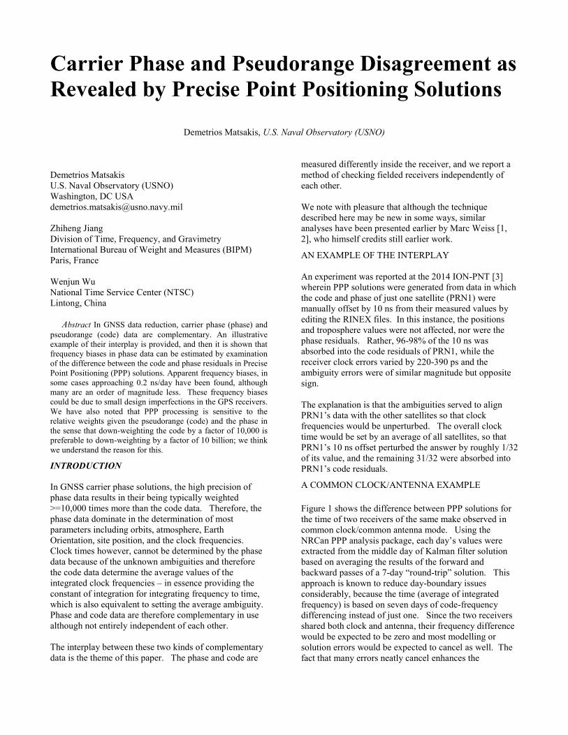
Figure 28 shows that NIST and IP02 (in Portugal) have
the same east-west asymmetry in magnitude and sign.
However, their slopes are of opposite sense.
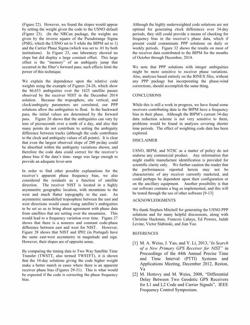
By comparing the timing data to Two Way Satellite Time
Transfer (TWSTT, also termed TWSTFT), it is shown
that the 34-day solutions giving the code higher weight
make a better match in cases where there is an apparent
receiver phase bias (Figures 29-31). This is what would
be expected if the code is correcting the phase frequency
bias.
Although the highly underweighted code solutions are not
optimal for generating clock differences over 34-day
periods, they still could provide a means of checking for
frequency bias in the receiver’s phase data, which if
present could contaminate PPP solutions on daily or
weekly periods. Figure 32 shows the results on most of
the receiver data contributed to the BIPM for the months
of October through December, 2014.
We note that PPP solutions with integer ambiguities
might be more sensitive to receiver phase variations.
Also, analyses based entirely on the RINEX files, without
any PPP package but incorporating the phase-wind
corrections, should accomplish the same thing.
CONCLUSIONS
While this is still a work in progress, we have found some
receivers contributing data to the BIPM have a frequency
bias in their phase. Although the BIPM’s current 34-day
data reduction scheme is not very sensitive to them,
problems would be found in analyses covering shorter
time periods. The effect of weighting code data has been
explored.
DISCLAIMER
USNO, BIPM, and NTSC as a matter of policy do not
endorse any commercial product. Any information that
might enable manufacture identification is provided for
scientific clarity only. We further caution the reader that
the performances reported herein may not be
characteristic of any receiver currently marketed, and
could perhaps be dependent upon their configuration or
on the ancillary equipment. Another possibility is that
our software contains a bug as implemented, and this will
be tested through the use of other software [9-13]
ACKNOWLEDGMENTS
We thank Stephen Mitchell for generating the USNO PPP
solutions and for many helpful discussions, along with
Christine Hackman, Francois Lahaye, Ed Powers, Judah
Levine, Victor Slabinski, and Jian Yao.
REFERENCES
[1] M. A. Weiss, J. Yao, and Y. Li, 2013,“In Search
of a New Primary GPS Receiver for NIST” in
Proceedings of the 44th Annual Precise Time
and Time Interval (PTTI) Systems and
Applications Meeting, December 2012, Reston,
Va
[2] M. Hottovy and M. Weiss, 2008, “Differential
Delay Between Two Geodetic GPS Receivers
for L1 and L2 Code and Carrier Signals”, IEEE
Frequency Control Symposium.

[3] C. Hackman, 2014, “Mitigating the Impact of
Predicted-Satellite-Clock Errors on GNSS PPP
Positioning”, ION-ITM
[4] http://webapp.geod.nrcan.gc.ca/geod/tools-
outils/ppp.php.
[5] D. Matsakis, K. Senior, and P. Cook, 2002,
“Comparison of Continuously Filtered GPS
Carrier Phase Time Transfer with Independent
GPS Carrier-Phase Solutions and with Two-Way
Satellite Time Transfer,” in Proceedings of the
33rd
Annual Precise Time and Time Interval
(PTTI) Systems and Applications Meeting, 27-
29 November 2001, Long Beach, California,
USA (U.S. Naval Observatory, Washington,
D.C.), pp. 63-87
[6] J.T. Wu, S.c. Wu, G.A. Hajj, W.J. Bertiger, and
s.M. Litchen, 1993, “Effects of antenna
orientation on GPS carrier phase”, Man.
Geodetica 18, pp. 91-98.
[7] S. Datta-Barua, T. Walter, J. Blanch, and
P.Enge, 2008, “Bounding higher-order
ionosphere errors for the dual-frequency GPS
user,”, Radio science 43, RS5010
[8] S. Pireaux, P. Defraigne, L. Wauters, N.
Bergeot, Q. Baire, and C. Bruyninx, 2010,
“Higher-order ionospheric effects in GPS time
and frequency transfer”, GPS Solutins, 14(3),
267-277.
[9] J. Yao and J. Levine, 2013, “A New Algorithm
to Eliminate GPS Carrier-phase Time T ransfer
Boundary Discontinuity” ION-PTTI
[10] J. Yao and J. Levine, 2014, “An
Improvement of RINEX-Shift Algorithm for
Continuous GPS Carrier-Phse Time Transfer,
ION-GNSS
[10] J. Yao and J. Levine, 2014, “GPS
Measurements Anomaly and Continuous GPS
Carrier-Phase Time Transfer, ION-PTTI
[11] J. Yao, S. Ivan, and J. Levine, 2015,
“Comparison of Two Continuous GPS Carrier-
Phase Time Transfer Techniques”, 2015,
Proceedings IFCS/EFTF, Denver, Co., USA
[12]N. Guyennon, P. Defraigne, and C. Bruyninx,
2007, “PPP and phase-only gps time and
frequency transfer, 27th EFTF Proceedings, pp
904-908.
Figure 1. PPP clock difference between two geodetic receivers
Figure 2. Difference in slopes of satellite tracks at the L3 frequency (2.54*L-1.54*L2).
Each point represents the slope of a completed satellite track at its midpoint.

Figure 3. As in previous figure, except the differences in the slopes of the
completed satellite tracks are at the L1 frequency.
Figure 4. As in previous figure, except the difference in the slopes of the
completed satellite tracks is at the L2 frequency.

Figure 5. As with figure 2, except but with receiver pairs Y and Z
Figure 6. As with figure 2, except with receiver pair X and Z

Figures 7-20 show daily slopes in code-phase from individual receivers. Unit 38 is “Y” in Figures 2-5.


Figure 21. Average slope of code-phase, over all complete satellite tracks, for each receiver studied. All units between
two vertical markers have a common manufacturer. One-sigma limits are indicated by the continuous curves;
therefore the large variations in units 24 and 25 are not significant. Unit 38 is receiver “Y” in figures 2-5, and is based
only upon data since the firmware upgrade.

Figure 22. Code-Phase Residuals for many laboratories in 34-day solutions covering the month of December, 2014. None
of them display a large systematic slope, although some of those were found to have them in the USNO’s 7-day solutions.
Figure 23. Code-Phase residuals using the same processing as the previous figure, except that the weight of the code was
decreased by a factor of one million. Note that three laboratories now display a systematic frequency offset. The large
constant offset of one laboratory is the memory of an ambiguity jump in the forward pass.

Figure 24 Ambiguities from all observations, backwards direction. The red points were offset for display.
Figure 25. A section of previous figure.

Figure 26. A very small portion of the previous figure. The solution proceeds in the backwards direction, so the
intial ambiguities initially vary considerably as the approach maturity. The final ambiguities are not applied to the
entire satellite track in these solutions.
Figure 27. Code-phase residuals in the easterly and westerly directions for the receiver with IGS designation NIST, and their
almost-constant difference.
\
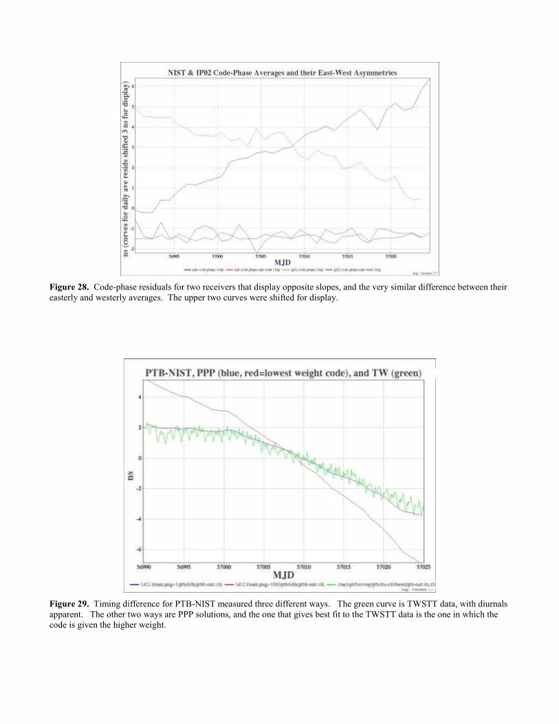
Figure 28. Code-phase residuals for two receivers that display opposite slopes, and the very similar difference between their
easterly and westerly averages. The upper two curves were shifted for display.
Figure 29. Timing difference for PTB-NIST measured three different ways. The green curve is TWSTT data, with diurnals
apparent. The other two ways are PPP solutions, and the one that gives best fit to the TWSTT data is the one in which the
code is given the higher weight.
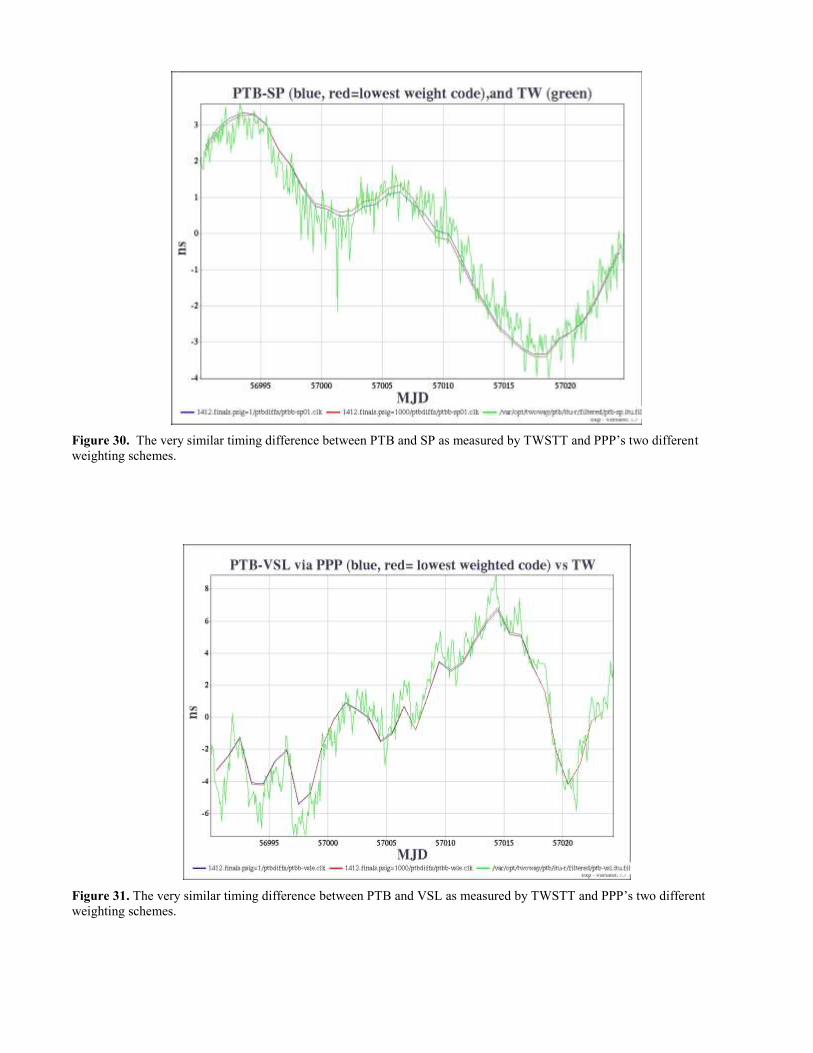
Figure 30. The very similar timing difference between PTB and SP as measured by TWSTT and PPP’s two different
weighting schemes.
Figure 31. The very similar timing difference between PTB and VSL as measured by TWSTT and PPP’s two different
weighting schemes.

Figure 32. Slope of residuals in solutions for October, November, and December 2014. Receivers between vertical
markers are of the same time. Each receiver has a unique abscissa-value. If all three months provided reasonable
data there will be three points for that receiver. The formal errors are comparable to the dot size. A spread between
points for the same receiver could indicate a change of that receiver’s properties.