arX

iv:1

606.

0885

2v1

[as

tro-

ph.G

A]

28

Jun

2016

CARMA LARGE AREA STAR FORMATION SURVEY: DENSE GAS IN THE

YOUNG L1451 REGION OF PERSEUS

Shaye Storm1,2, Lee G. Mundy2, Katherine I. Lee1,2, Manuel Fernandez-Lopez3,4, Leslie W. Looney3, PeterTeuben2, Hector G. Arce5, Erik W. Rosolowsky6, Aaron M. Meisner 7, Andrea Isella8, Jens Kauffmann9,Yancy L. Shirley10, Woojin Kwon11, Adele L. Plunkett12, Marc W. Pound2, Dominique M. Segura-Cox3,

Konstantinos Tassis13,14, John J. Tobin15, Nikolaus H. Volgenau16, Richard M. Crutcher3, Leonardo Testi17

Accepted to The Astrophysical Journal (ApJ); June 25, 2016

(see published version for full-resolution figures)

ABSTRACT

We present a 3 mm spectral line and continuum survey of L1451 in the Perseus MolecularCloud. These observations are from the CARMA Large Area Star Formation Survey (CLASSy),which also imaged Barnard 1, NGC 1333, Serpens Main and Serpens South. L1451 is the surveyregion with the lowest level of star formation activity—it contains no confirmed protostars. HCO+,HCN, and N2H

+ (J = 1 → 0) are all detected throughout the region, with HCO+ the most spatiallywidespread, and molecular emission seen toward 90% of the area above N(H2) column densities of1.9×1021 cm−2. HCO+ has the broadest velocity dispersion, near 0.3 km s−1 on average, comparedto ∼0.15 km s−1 for the other molecules, thus representing a range from supersonic to subsonic gasmotions. Our non-binary dendrogram analysis reveals that the dense gas traced by each molecule hassimilar hierarchical structure, and that gas surrounding the candidate first hydrostatic core (FHSC),L1451-mm, and other previously detected single-dish continuum clumps have similar hierarchicalstructure; this suggests that different sub-regions of L1451 are fragmenting on the pathway toforming young stars. We determined the three-dimensional morphology of the largest detectable

1Harvard-Smithsonian Center for Astrophysics, 60 Garden Street, Cambridge, MA 02138, USA

2Department of Astronomy, University of Maryland, College Park, MD 20742, USA; sstorm@astro.umd.edu

3Department of Astronomy, University of Illinois at Urbana–Champaign, 1002 West Green Street, Urbana, IL 61801, USA

4Instituto Argentino de Radioastronomıa, CCT-La Plata (CONICET), C.C.5, 1894, Villa Elisa, Argentina

5Department of Astronomy, Yale University, P.O. Box 208101, New Haven, CT 06520-8101, USA

6University of Alberta, Department of Physics, 4-181 CCIS, Edmonton AB T6G 2E1, Canada

7Lawrence Berkeley National Laboratory and Berkeley Center for Cosmological Physics, Berkeley, CA 94720, USA

8Physics & Astronomy Department, Rice University, P.O. Box 1892, Houston, TX 77251-1892, USA

9Max Planck Institut fur Radioastronomie, Auf dem Hugel 69 D53121, Bonn Germany

10Steward Observatory, 933 North Cherry Avenue, Tucson, AZ 85721, USA

11Korea Astronomy and Space Science Institute,776 Daedeok-daero, Yuseong-gu, Daejeon 305-348, Republic of Korea

12European Southern Observatory, Av. Alonso de Cordova 3107, Vitacura, Santiago de Chile

13Department of Physics and Institute of Theoretical & Computational Physics, University of Crete, PO Box 2208, GR-710 03, Heraklion, Crete, Greece

14Foundation for Research and Technology - Hellas, IESL, Voutes, 7110 Heraklion, Greece

15Leiden Observatory, 540 J.H. Oort Building, Niels Bohrweg 2, NL-2333 CA Leiden, The Netherlands

16Las Cumbres Observatory Global Telescope Network, Inc. 6740 Cortona Drive, Suite 102 Goleta, CA 93117, USA

17ESO, Karl-Schwarzschild-Strasse 2 D-85748 Garching bei Munchen, Germany

– 2 –

dense gas structures to be relatively ellipsoidal compared to other CLASSy regions, which appearedmore flattened at largest scales. A virial analysis shows the most centrally condensed dust structuresare likely unstable against collapse. Additionally, we identify a new spherical, centrally condensedN2H

+ feature that could be a new FHSC candidate. The overall results suggest L1451 is a youngregion starting to form its generation of stars within turbulent, hierarchical structures.

1. Introduction

The star formation process in a molecular cloud starts well before protostars are detectable at infraredwavelengths. In general, it begins with the formation of the molecular cloud that may span tens of parsecs (Evans1999; Elmegreen & Scalo 2004; McKee & Ostriker 2007); it continues as structure and density enhancements arecreated by the interaction of turbulence, gravity, and magnetic fields at parsec scales (McKee & Ostriker 2007;Crutcher 2012), and it progresses until prestellar core collapse occurs at 0.01–0.1 pc scales (di Francesco et al.2007; Bergin & Tafalla 2007). Once a first generation of protostars is formed within those dense cores, the youngstars can feed energy back into the cloud and impact subsequent star formation that may occur (Nakamura & Li2007; Carroll et al. 2009; Nakamura & Li 2014). A full understanding of how turbulence, gravity, and magneticfields control the star formation process requires observations that span cloud to core spatial scales at thesedistinct evolutionary stages.

An individual molecular cloud can be a great testbed for studying the star formation process across spaceand time if it is sufficiently close to get better than 0.1 pc resolution, and if it contains regions with distinctevolutionary stages. The Perseus Molecular Cloud is a nearby example of such a cloud. The regions of Perseuswith infrared detections of young stellar objects (YSOs) span a range of evolutionary epochs based on YSOstatistics from the c2d Legacy project (Jørgensen et al. 2008; Evans et al. 2009). For example, the IC 348region has 121 YSOs, with 9.1% being Class I or younger; the NGC 1333 region has 102 YSOs, with 34% beingClass I or younger; Barnard 1 region has 9 YSOs, with 89% being Class I or younger. Regions without currentprotostellar activity also exist within Perseus. The B1-E region may be forming a first generation of densecores (Sadavoy et al. 2012), and the L1451 region has a single detection of a compact continuum core, which isa candidate first hydrostatic core (FHSC) (Pineda et al. 2011).

The CARMA Large Area Star Formation Survey (CLASSy) observed the dense gas in three evolu-tionary distinct regions within Perseus (Storm et al. 2014) and two regions within Serpens (Lee et al. 2014;Fernandez-Lopez et al. 2014) with high angular and velocity resolution. The observations enable a high reso-lution study of the structure and kinematics of star forming material at different epochs. From early to latestages of evolution (based on the ratio of Class II and older to Class I and younger YSOs), the Perseus regionsof CLASSy are L1451, Barnard 1, and NGC 1333. The youngest region, L1451, probes cloud conditions duringthe origin of clumps and stars; the more evolved Barnard 1 region probes cloud conditions when a relativelysmall number of protostars are formed, and the active NGC 1333 region probes cloud conditions when dozensof clustered protostars are driving outflows back into the cloud. Details of CLASSy, along with an analysis ofBarnard 1, can be found in Storm et al. (2014) (referred to as Paper I in the sections below).

This paper focuses on the L1451 region. L1451 is located ∼5.5 pc to the southwest of NGC 1333 (seeFigure 1 of Paper I). The region has been surveyed at a number of wavelengths as reported in the literatureand summarized below. It contains no Spitzer -identified YSOs at IRAC or MIPS wavelengths (Jørgensen et al.2008)1. Hatchell et al. (2005) and Kirk et al. (2006) did not identify any cores in their JCMT SCUBA 850 µmsurvey. There are four 1.1 mm sources identified in the Bolocam Survey (Enoch et al. 2006) that are classifiedas “starless” cores in Enoch et al. (2008): PerBolo 1, 2, 4, and 6. Pineda et al. (2011) used 3 mm CARMA and

1The Spitzer c2d YSO sample is 90% complete down to 0.05 L⊙ for clouds at 260 pc (Evans et al. 2009).

– 3 –

1.3 mm SMA observations to show that PerBolo 2 is not a starless core, but likely a core with an embeddedYSO or a FHSC.

The Bolocam cores within L1451 are colder and less dense than the average Bolocam cores within Perseus.The visual extinction (AV ) of the four Bolocam sources ranges from 8 to 11 magnitudes, while the mean andmedian AV for all Perseus sources are 24.6 and 12, respectively (Enoch et al. 2006). The mean particle densityof the L1451 Bolocam sources ranges from 0.9 × 105 to 1.5 × 105 cm−3, which is lower than the mean densityfor all Perseus sources of 3.2 × 105 (Enoch et al. 2008). The kinetic temperature of gas within the L1451 coresranges from 9.1 to 10.3 K, which is lower than the mean for all Perseus cores of 11.0 (Rosolowsky et al. 2008a).These statistics complement the YSO statistics that suggest L1451 it is at an earlier evolutionary epoch thanBarnard 1 and NGC 1333.

The main science goals of our large-area, high-resolution, spectral line observations of this young region are:1) to quantify the dense gas content of a cloud region possibly at the onset of star formation, 2) to determinewhether complex, hierarchical structure formation exists before the onset of star formation, as predicted bytheories of turbulence-driven star formation, 3) to better understand how natal cloud material fragments onthe pathway to star formation, by quantifying the hierarchical similarities and differences between sub-regionsof L1451 with and without compact cores, 4) to estimate the boundedness of the dense structures in young starforming regions, and 5) to potentially discover new young cores.

The paper is organized as follows. Section 2 provides an overview of CLASSy observations of L1451.Properties of the L1451-mm continuum detection are in Section 3. Section 4 presents the dense gas morphologyusing integrated intensity and channel maps, and Section 5 presents the dense gas kinematic results from spectralline fitting. A dendrogram analysis of the HCO+, HCN, and N2H

+ data cubes is in Section 6. Section 7 showshow we calculate column density, dust temperature, and extinction maps using Herschel data, along with adendrogram analysis of the extinction map. Section 8 discusses the current state of star formation in L1451using the spectral line data in combination with the continuum data to further quantify physical and spatialproperties of structures in L1451. We summarize our key findings in Section 9.

2. Observations

The details of CLASSy observations, calibration, and mapping are found in Paper I; specifics related toL1451 are summarized here. We mosaicked a total area of ∼150 square arcminutes in CARMA23 mode, whichuses all 23 CARMA antennas. The mosaic was made up of two adjacent rectangles, containing a total of 673individual pointings with 31′′ spacing in a hexagonal grid (see Figure 1). The reference position of the mosaic isat the center of the eastern rectangle: α=03h25m17s, δ=30◦21′23′′(J2000). The L1451-mm core (Pineda et al.2011) is within the eastern rectangle. The region was observed for 150 total hours, split between the DZ andEZ configurations, which provide projected baselines from about 1–40 kλ and 1–30 kλ, respectively, and ahybrid array (DEZ) with baselines ranging from about 1–35 kλ. The DEZ array was not used for the CLASSyobservations presented in Paper I, and is the reason the synthesized beam for L1451 is slightly larger thanthat for Barnard 1. See Table 1 for a summary of observing dates and calibrators. The mapped region coversroughly 1.1 pc by 0.6 pc with about 1800 AU spatial resolution.

The correlator setup is summarized in Table 2. N2H+, HCO+, and HCN (J = 1 → 0) were simultaneously

observed in 8 MHz bands, providing a velocity resolution of 0.16 km s−1. We also used a 500 MHz bandfor continuum observations and calibration. Data were inspected and calibrated using MIRIAD (MultichannelImage Reconstruction, Image Analysis and Display; Sault et al. 1995) as described in Paper I. 3C84 was observedevery 16 minutes for gain calibration; 3C111 was used for gain calibration when 3C84 transited above 80 degreeselevation. Uranus was observed for absolute flux calibration. The flux of 3C84 varied between 16 and 21 Jy overthe observing period, while 3C111 varied between 2.6 and 4.5 Jy. The uncertainty in absolute flux calibration

– 4 –

Fig. 1.— A Herschel image of the 250 µm emission (yellow is brighter emission, red is fainter emission) from L1451with the CLASSy mosaic pointing centers overlaid as white points. The spacing of the pointing centers is 31′′, and ourtotal area coverage is ∼150 square arcminutes. The locations of 1.1 mm Bolocam sources (Enoch et al. 2006) and theL1451-mm compact continuum core (Pineda et al. 2011) are marked with black squares and a black star, respectively.

is about 10%. We will only report statistical uncertainties when quoting errors in measured values throughoutthe paper.

To create spectral-line images which fully recover emission at all spatial scales, CARMA observed in single-dish mode during tracks with stable atmospheric opacity. The OFF position for L1451 was 3.5′ west and 13.7′

south of the mosaic reference position, at the location of a gap in 12CO and 13CO emission to ensure nosignificant dense gas contribution. The single-dish data from the 10.4-m dishes was calibrated in MIRIAD asdescribed in Paper I. The antenna temperature rms in the final single-dish cubes was ∼0.02 K for all threemolecules. The spectral-line interferometric and single-dish data were combined with mosmem, a maximumentropy joint deconvolution algorithm in MIRIAD. The noise levels and synthesized beams for the final datacubes are given in Table 2. The rms noise in these lines correspond to brightness temperature rms of 0.34 Kfor N2H

+ and 0.30 K for HCO+ and HCN.

We created a 3 mm continuum map with the interferometric data from the 500 MHz window. The rms inthe continuum map is ∼1.3 mJy beam−1 with a synthesized beam of 9.2′′ × 6.6′′. Single-dish continuum datacan not be acquired at CARMA.

Table 1. Observation Summary

Array Dates Total Hours Flux Cal. Gain Cal. Mean Flux (Jy)

DZ October 2012 25 Uranus 3C84/3C111 18.6/2.6April – June 2013 19 Uranus 3C84/3C111 17.1/2.7

DEZ February 2013 31 Uranus 3C84/3C111 20.7/3.9EZ August – September 2012 25 Uranus 3C84/3C111 18.0/3.1

July – August 2013 50 Uranus 3C84/3C111 17.5/4.2

– 5 –

3. Continuum Results

We detected no compact continuum sources above the 5σ level of the 3 mm continuum map. One sourcewas detected above 3σ that could be confirmed with other observations; L1451-mm (Pineda et al. 2011) isdetected at 4σ with 5.2 mJy beam−1. Figure 2 shows the 3 mm continuum image toward L1451-mm. Theposition, peak brightness, and lower-limit mass for our detection were calculated following the prescriptiondescribed in Paper I and are listed in Table 3. The position and peak brightness agree with CARMA 3 mmmeasurements from Pineda et al. (2011), which had a ∼5′′ synthesized beam. Our image shows a possiblesecondary peak to the north of the brightest emission. However, this secondary peak is only within the 2–3σcontours and does not appear in the higher sensitivity observations of Pineda et al. (2011). Pineda et al. (2011)detected a low-velocity CO (J = 2 → 1) outflow in this area; we do not detect any HCN or HCO+ outflowemission near this source.

Fig. 2.— The single continuum detection in our field. The synthesized beam is 9.2′′ × 6.6′′, and the 1σ sensitivity is1.3 mJy beam−1. The contour levels are 2, 3 times 1σ; no negative contours are present.

4. Morphology of Dense Molecular Gas

4.1. Integrated Intensity Emission

Figure 3 shows integrated intensity maps for HCO+, HCN, and N2H+ (J = 1 → 0) (∼8′′ angular reso-

lution), along with a Herschel 250 µm image (18.1′′ angular resolution) for a visual comparison between the

Table 2. Correlator Setup Summary

Line Rest Freq. No. Chan. Chan. Width Vel. Coverage Vel. Resolution Chan. RMS Synth. Beama

(GHz) (MHz) (km s−1) (km s−1) (Jy beam−1)

N2H+ 93.173704b 159 0.049 24.82 0.157 0.14 8.6′′ × 6.8′′

Continuum 92.7947 47 10.4 1547 33.6 0.0013 9.2′′ × 6.6′′

HCO+ 89.188518 159 0.049 25.92 0.164 0.12 8.8′′ × 7.1′′

HCN 88.631847c 159 0.049 26.10 0.165 0.12 8.9′′ × 7.2′′

Note. — aThe synthesized beam is slightly different for each pointing center, and MIRIAD calculates a synthesized

beam for the full mosaic based on all of the pointings. bThe rest frequency of the band was set to the weighted meanfrequency of the center three hyperfine components. cThe rest frequency of the band was set to the frequency of the

center hyperfine component. See http://splatalogue.net for frequencies of the HCN and N2H+ hyperfine components.

– 6 –

dense gas and dust emission. The line maps were integrated over all channels with identifiable emission. Thelocations of the four Bolocam 1.1 mm sources (Enoch et al. 2006) and the one compact continuum core inL1451 are marked on each image of Figure 3. Four of the five sources are located near peaks of dense gas anddust emission. While the molecules and dust are tracing similar features around those sources, the exact mor-phological details vary. Below, we describe the qualitative emission features, and refer to the colored rectanglesin Figure 3 for reference.

All tracers show a curved structure surrounding L1451-mm and the two nearby Bolocam sources (see redrectangle in Figure 3), with a peak of integrated emission at the location of L1451-mm. The southwesternedge of the curved structure has a stream of emission that extends further to the southwest (see dark bluerectangle in upper left panel of Figure 3), which can be seen in all the maps, though it extends furthest in theHCO+, HCN, and dust maps. The two other Bolocam sources to the far east of L1451-mm are surroundedby significant molecular gas structure (see green rectangle in lower left panel). The HCO+ emission has thelargest spatial extent in this region.

The integrated emission in the three lines is less similar across the western half of L1451 compared to theeastern half. There is a strong, condensed N2H

+ source (see orange rectangle in lower right panel) that does notappear strongly in the HCN or HCO+ maps, but that does correspond to a peak of emission in the dust map(see Section 8.3 for more details on this source). The strongest HCO+ feature in the western half of the maphas a weaker counterpart in the HCN map (see purple rectangle), which appears even weaker in N2H

+. Finally,there is HCO+ emission to the northwest of the curved structure (see cyan rectangle) that closely mimics dustemission in that region; this emission is weakly detected in HCN, but not in N2H

+. Since the J = 1 → 0transition of HCO+ traces densities about an order of magnitude lower than the other two molecules (Shirley2015), the regions with strong HCO+ and weak HCN and N2H

+ are likely at lower density compared to regionswhere all the molecules have strong emission.

4.2. Channel Emission

Figure 4 shows channel maps of HCO+, HCN, and N2H+ highlighting the bulk of the emission, which

occurs from ∼4.8 to 3.5 km s−1, with 2-channel spacing (e.g., we skip the 4.66 km s−1 channel between the4.82 km s−1 and 4.50 km s−1 channels of HCO+). In general, it is clear from the channel maps in Figure 4that strong HCO+ emission is more widespread compared to HCN emission, and particularly N2H

+ emission(as was also evident in Figure 3). We label qualitative features in the HCO+ channel maps, from A throughI, in the order that they appear in velocity space (with eastern sources being labeled before western sources).We then place those same labels on the HCN and N2H

+ maps to aid a qualitative comparison of dense gasfeatures, given below.

Features A and C in the eastern half of the map are traced with all molecules, with varying strength. InFigure 4, Feature A appears strongly in HCO+ at 4.82 km s−1, faintly at 4.82 km s−1 in HCN, and not until

Table 3. Observed Properties of Continuum Detection

Source Position Pk. Bright. MassName (h:m:s, d:′:′′) (mJy beam−1) (M⊙)(1) (2) (3) (4)

L1451-mm 03:25:10.38, +30:23:55.9 5.2 ± 1.3 0.10 ± 0.03

Note. — (3) Peak brightness, (4) Lower-limit mass using the peak brightness andassumptions outlined in Paper I.

– 7 –

Fig. 3.— Integrated intensity maps of HCO+, HCN, and N2H+(J = 1 → 0) emission toward L1451, along with a Herschel

250 µm map of the region. HCO+ emission was integrated from 5.316 to 3.018 km s−1. HCN emission was integratedover all three hyperfine components from 9.945 to 7.962 km s−1, 5.154 to 2.841 km s−1, and −2.115 to −3.932 km s−1.N2H

+ emission was integrated over all seven hyperfine components over velocity ranges from 11.542 to 8.714 km s−1,5.729 to 2.744 km s−1, and −3.383 to −4.639 km s−1. The rms of the maps are 0.08, 0.13, and 0.16 Jy beam−1 km s−1 forHCO+, HCN, and N2H

+, respectively. The four Bolocam 1.1 mm sources in this region are marked with “x” symbols, andthe L1451-mm compact continuum core is marked with an asterisk. Colored rectangles show the locations of qualitativefeatures discussed in Section 4.1.

4.47 km s−1 in N2H+. Even when it finally appears as N2H

+ emission, the emission is much more spatiallyconcentrated than what we observe in HCO+ and HCN. This spatial concentration is likely because the N2H

+

(J = 1 → 0) line traces higher-density, colder material compared to HCO+ and HCN (J = 1 → 0) lines (Shirley2015). A 1.1 mm Bolocam core is located within Feature A, and corresponds with a peak in the N2H

+ emission.Feature A moves northeast to southwest from 4.82 km s−1 to lower-velocity channels as Feature C appears toits southwest. Features A and C are possibly part of the same larger-scale structure, which will be explored inthe next section when we analyze the kinematics of this region. Like Feature A, Feature C is more spatiallyconcentrated in N2H

+, and contains a 1.1 mm Bolocam source at an N2H+ peak of emission.

Feature B contains the L1451-mm compact continuum source. It appears strongly in all molecules, thoughit contains a prominent ridge of emission at 4.82 km s−1 in HCO+ and HCN that does not appear in N2H

+

near that velocity.

Features D, E, F, G, H, and I are all identified based on the HCO+ emission. HCN emission appears weaklytoward all features seen with HCO+, while N2H

+ only shows faint emission in one channel for Features G andH at 3.84 km s−1. The descriptions below are based on HCO+. Feature D appears to the west of FeaturesA and C, and to the south of Feature B, seen at 4.50 km s−1 as an elliptical feature. Feature E appears asa prominent, round emission feature at 4.50 km s−1, with more extended emission in channels surroundingthe 4.50 km s−1 peak of emission. Feature F is emission that starts just to the northwest of Feature B at

– 8 –

4.17 km s−1, peaks at 3.83 km s−1, and then appears to get fainter while extending to the southwest at theunshown 3.67 km s−1 channel, while then brightening to the southwest at 3.51 km s−1. Feature G emissionpeaks at 3.83 km s−1, and appears as a stream of emission to the east of Feature E. Feature H is a streamerto the southwest of Feature B and the south of Feature F, which first appears at 3.83 km s−1. It persists at3.51 km s−1 and more faintly extends into two lower-velocity channels not shown in the figure. Feature I firstappears at 3.51 km s−1, brightens in two lower-velocity channels not shown in the figure, and is not detectableat velocities lower than that.

Feature J, referred to as L1451-west in the rest of the paper, is relatively round emission that only appearsstrongly in the N2H

+ data. It first appears at 4.79 km s−1 in Figure 4, and is visible across a total offour velocity channels per hyperfine component—the structure can be seen repeating for another hyperfinecomponent, starting in the 3.84 km s−1 channel. We discuss details of the structure and kinematics of L1451-west in Section 8.3.

We detect no HCN or HCO+ outflow emission in any channel, which suggests that L1451 is a young regionwith little to no protostellar activity. Figure 5 show an example spectrum for each molecule from the locationof L1451-mm within a single synthesized beam. The conversions from Jy beam−1 to K for these data are2.47 K/Jy beam−1, 2.46 K/Jy beam−1, and 2.42 K/Jy beam−1 for HCO+, HCN, and N2H

+, respectively.

A small fraction of HCO+ and HCN spectra across L1451 show double peaks with a variety of line-shapecharacteristics—we estimate that ∼3% of cloud locations show double-peak features. We cannot determinethe absolute cause of the double peaks without H13CN and H13CO+ (J = 1 → 0) observations at each cloudlocation, so analyzing these features is beyond the scope of this paper. However, the most likely scenario isself-absorption from a foreground screen of lower-density gas with a significant HCO+ and HCN (J = 1 → 0)population. An infall scenario can be ruled out in many locations since infall predicts a stronger blue peak(Evans 1999) while we often observe stronger red peaks; a scenario with two-components along the sameline-of-sight can likely be ruled out in many locations where the HCO+ and HCN spectra do not both showdouble-peaks.

– 9 –

Fig. 4.— Left : Five HCO+ channels maps, with two-channel spacing. The rms in each channel is 0.12 Jy beam−1, andthe color intensity ranges from 0.12–1.3 Jy beam−1. Features discussed in the text are identified with a letter in thefirst channel they appear. Center : Five HCN channels maps. The rms in each channel is 0.12 Jy beam−1, and the colorintensity ranges from 0.12–0.9 Jy beam−1. Feature labels from the HCO+ maps are overplotted in the same locationsfor aid in comparing the emission across molecules. Right : Five N2H

+ channel maps. Note that several features appeartwice across the channels due to the hyperfine structure of N2H

+. The rms in each channel map is 0.14 Jy beam−1, andthe color intensity ranges from 0.14–0.9 Jy beam−1. Feature labels from the HCO+ maps are overplotted in the samelocations for aid in comparing the emission across molecules. Feature J (also referred to as L1451-west) only appears inN2H

+, so it is only labeled in this figure.

– 10 –

Fig. 5.— Example HCO+, HCN, and N2H+ spectra from the location of L1451-mm reported in Table 3. Spectra are

averaged over one synthesized beam, and the conversion factors from Jy beam−1 to Kelvin are reported in the text.

– 11 –

5. Kinematics of Dense Molecular Gas

We fitted the molecular line emission presented in Section 4 with Gaussians using the method described inPaper I, and present the centroid velocity and line-of-sight velocity dispersion maps here. The seven resolvablehyperfine components of the N2H

+ (J = 1 → 0) line, and the three hyperfine components of the HCN (J =1 → 0) line, are simultaneously fit assuming the same velocity dispersion and excitation conditions for eachcomponent. HCO+ (J = 1 → 0) has no hyperfine splitting and is fit as a single Gaussian component.

We fit all the HCN and HCO+ spectra with a single component across the entire field, even though about3% of the spectra show evidence of double-peaks. To estimate the impact of fitting a double-peaked spectrumwith a single component, we extrapolated several double-peaked spectra to a single peak, fit those single-peakspectra, and measured the full width at half of the extrapolated single-peak spectra. From those fits, we estimatethat the velocity dispersions derived from the single-component fits to double-peaked spectra are overestimatedby ∼10%. Considering that only about 3% of the spectra have this 10% overestimation, the double-peaks havea negligible impact on the results presented in this paper.

Although a low-velocity outflow from L1451-mm was previously detected in CO (J = 2 → 1) by Pineda et al.(2011), we do not detect any outflow signatures in our HCN or HCO+ (J = 1 → 0) observations as we did inother CLASSy fields. Therefore, there are no line broadening effects from outflows that are impacting the lineprofile fits.

In Figure 6, we plot the fitted centroid velocity and velocity dispersion where: 1) the integrated intensityis greater than or equal to four times the rms of the integrated intensity map, and 2) the peak signal-to-noiseof the spectrum is greater than five. We will use these kinematic maps in the following sections in order tointerpret the hierarchical and turbulent nature of the region. Here we list some general features of interestpertaining to the maps:

1. HCO+ has systematically larger line-of-sight velocity dispersion compared to HCN and N2H+. The mean

and standard deviation of the velocity dispersions across the maps are 0.29 ± 0.10, 0.16 ± 0.07, and0.12 ± 0.04 km s−1, for HCO+, HCN, and N2H

+, respectively. The observed mean velocity dispersionsabove should be compared to the isothermal sound speed of the mean gas particles in the cloud fordetermining the turbulence in the observed gas. Note that the thermal velocity dispersion of the meangas particle in the cloud is different from the thermal velocity dispersion of an individual molecule. If weassume that the typical temperature in this region is 10 K based on ammonia observations of Bolocamcores (Rosolowsky et al. 2008a), then the isothermal sound speed between the mean gas particles wouldbe ∼0.2 km s−1 (assuming molecular weight per free particle of 2.33), while the isothermal sound speedbetween individual N2H

+ particles would be ∼0.05 km s−1.

The N2H+ velocity dispersions are subsonic everywhere, the HCN velocity dispersions are subsonic in most

cloud locations, and the HCO+ velocity dispersions are transsonic to supersonic in most cloud locations.Note that even though N2H

+ and HCN are subsonic in many areas of L1451, they are not exhibitingpurely thermal velocity dispersions, which would be ∼0.05 km s−1 for 10 K gas. The J = 1 → 0 lineof HCO+ traces densities about an order of magnitude lower than that of HCN and N2H

+ (see Shirley2015). Therefore, we are likely observing the trend from supersonic to subsonic gas motions as gas goesfrom the larger, less-dense scales traced by HCO+ to the smaller, more-dense scales traced by HCN andN2H

+. This is expected in a turbulent medium, where velocity dispersion scales proportionally with size(McKee & Ostriker 2007).

2. All three molecules are tracing gas with centroid velocities ranging from ∼3.8–4.7 km s−1. However, theHCO+ gas extends to lower velocities, due to the gas in the Feature H streamer, which appears in theHCN maps, but is not strong enough to provide reliable kinematic measurements. HCO+ also extends to

– 12 –

higher velocities, due to strong gas emission from the northeast part of Feature A, which is noticeable inthe first channel of Figure 4.

3. The HCO+ centroid velocities for Features A and C show a gradient from northeast to southwest. It ispossible that this is a large, rotating piece of dense gas, which is fragmenting into denser components (e.g.,the Bolocam 1 mm sources). It is also possible that the redshifted northeast section and the blueshiftedsouthwest section represent independent components in the turbulent medium, or that they are merelyprojected along the same line of sight. Observations of optically thin tracers, and tracers of lower-density,larger-scale material are needed to help distinguish between these scenarios.

4. The gas in the eastern half of Feature B shows a velocity gradient along the length of the feature. It ismost blueshifted at the southeastern end near the L1451-mm core, and becomes increasingly redshiftedfurther away to the northwest. The gas immediately surrounding the L1451-mm compact continuumcore has a centroid velocity pattern that is consistent with rotation (Pineda et al. 2011), and has velocitydispersions that increase toward the core center. L1451-west N2H

+ velocity dispersions also peak at thecore center, and we compare these two sources in detail in Section 8.3.

5. Our measurements of N2H+ centroid velocity and velocity dispersion towards L1451-mm agree well with

the results in Pineda et al. (2011), in terms of absolute values measured and gradients across the source.

Fig. 6.— Kinematics of dense gas in L1451. Left: Centroid velocity (km s−1) maps of HCO+, HCN, and N2H+

(J = 1 → 0) emission, from top to bottom. Right: Line-of-sight velocity dispersion (FWHM/2.355 in km s−1) maps ofHCO+, HCN, and N2H

+ (J = 1 → 0) emission, from top to bottom. We masked these maps to visualize only statisticallyrobust kinematic results (see Section 5 text). The color scales are the same across molecules.

– 13 –

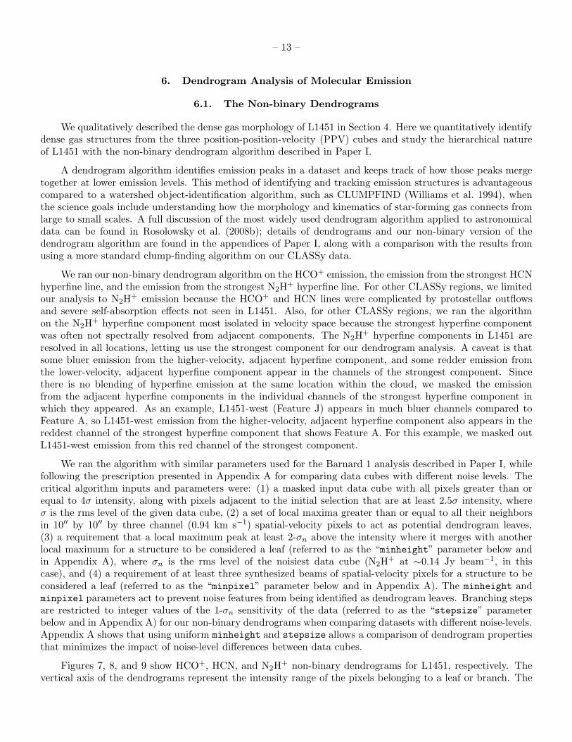
6. Dendrogram Analysis of Molecular Emission

6.1. The Non-binary Dendrograms

We qualitatively described the dense gas morphology of L1451 in Section 4. Here we quantitatively identifydense gas structures from the three position-position-velocity (PPV) cubes and study the hierarchical natureof L1451 with the non-binary dendrogram algorithm described in Paper I.

A dendrogram algorithm identifies emission peaks in a dataset and keeps track of how those peaks mergetogether at lower emission levels. This method of identifying and tracking emission structures is advantageouscompared to a watershed object-identification algorithm, such as CLUMPFIND (Williams et al. 1994), whenthe science goals include understanding how the morphology and kinematics of star-forming gas connects fromlarge to small scales. A full discussion of the most widely used dendrogram algorithm applied to astronomicaldata can be found in Rosolowsky et al. (2008b); details of dendrograms and our non-binary version of thedendrogram algorithm are found in the appendices of Paper I, along with a comparison with the results fromusing a more standard clump-finding algorithm on our CLASSy data.

We ran our non-binary dendrogram algorithm on the HCO+ emission, the emission from the strongest HCNhyperfine line, and the emission from the strongest N2H

+ hyperfine line. For other CLASSy regions, we limitedour analysis to N2H

+ emission because the HCO+ and HCN lines were complicated by protostellar outflowsand severe self-absorption effects not seen in L1451. Also, for other CLASSy regions, we ran the algorithmon the N2H

+ hyperfine component most isolated in velocity space because the strongest hyperfine componentwas often not spectrally resolved from adjacent components. The N2H

+ hyperfine components in L1451 areresolved in all locations, letting us use the strongest component for our dendrogram analysis. A caveat is thatsome bluer emission from the higher-velocity, adjacent hyperfine component, and some redder emission fromthe lower-velocity, adjacent hyperfine component appear in the channels of the strongest component. Sincethere is no blending of hyperfine emission at the same location within the cloud, we masked the emissionfrom the adjacent hyperfine components in the individual channels of the strongest hyperfine component inwhich they appeared. As an example, L1451-west (Feature J) appears in much bluer channels compared toFeature A, so L1451-west emission from the higher-velocity, adjacent hyperfine component also appears in thereddest channel of the strongest hyperfine component that shows Feature A. For this example, we masked outL1451-west emission from this red channel of the strongest component.

We ran the algorithm with similar parameters used for the Barnard 1 analysis described in Paper I, whilefollowing the prescription presented in Appendix A for comparing data cubes with different noise levels. Thecritical algorithm inputs and parameters were: (1) a masked input data cube with all pixels greater than orequal to 4σ intensity, along with pixels adjacent to the initial selection that are at least 2.5σ intensity, whereσ is the rms level of the given data cube, (2) a set of local maxima greater than or equal to all their neighborsin 10′′ by 10′′ by three channel (0.94 km s−1) spatial-velocity pixels to act as potential dendrogram leaves,(3) a requirement that a local maximum peak at least 2-σn above the intensity where it merges with anotherlocal maximum for a structure to be considered a leaf (referred to as the “minheight” parameter below andin Appendix A), where σn is the rms level of the noisiest data cube (N2H

+ at ∼0.14 Jy beam−1, in thiscase), and (4) a requirement of at least three synthesized beams of spatial-velocity pixels for a structure to beconsidered a leaf (referred to as the “minpixel” parameter below and in Appendix A). The minheight andminpixel parameters act to prevent noise features from being identified as dendrogram leaves. Branching stepsare restricted to integer values of the 1-σn sensitivity of the data (referred to as the “stepsize” parameterbelow and in Appendix A) for our non-binary dendrograms when comparing datasets with different noise-levels.Appendix A shows that using uniform minheight and stepsize allows a comparison of dendrogram propertiesthat minimizes the impact of noise-level differences between data cubes.

Figures 7, 8, and 9 show HCO+, HCN, and N2H+ non-binary dendrograms for L1451, respectively. The

vertical axis of the dendrograms represent the intensity range of the pixels belonging to a leaf or branch. The

– 14 –

horizontal axis is arranged with the major features identified in Figure 4 progressing from east-to-west; welabel certain branches that are associated with major features, and we provide the numeric label for structuresreferred to in the upcoming discussion. The isolated leaves are presented in numerical order. The horizontaldotted line in each dendrogram represents an intensity cut at 2.5-σn that aids in cross-comparison of dendrogramstatistics (see Appendix A) and is discussed in Section 6.3.

The HCO+ dendrogram contains the largest number of structures, with 86 leaves and 27 branches. TheHCN dendrogram contains 33 leaves and 13 branches, while the N2H

+ dendrogram only contains 16 leavesand 6 branches. Leaves that peak at least 6-σn in intensity above the branch they merge directly into arecolored green and referred to as high-contrast leaves2. The strongest leaf for every molecule is at or near thelocation of L1451-mm in Feature B: Leaf 66 is the strongest structure in the HCO+ dendrogram, with a peakintensity of 2.78 Jy beam−1, leaf 30 is the strongest structure in the HCN dendrogram, with a peak intensityof 2.58 Jy beam−1, and leaf 10 is the strongest structure in the N2H

+ dendrogram, with a peak intensity of1.62 Jy beam−1.

Fig. 7.— The HCO+ non-binary dendrogram for L1451. The vertical axis represents the Jy beam−1 intensity for a givenlocation within the gas hierarchy. The horizontal axis is ordered so that features identified in Section 4 are generallyordered from east to west. Leaves and branches discussed in the text are labeled with their numerical identifier, andbranches associated with major features from Section 4 are marked with the feature letter. The leaves colored green peakat least 6-σn above their first merge level. The horizontal dotted line represents the 2.5-σn intensity cut above which wecalculate tree statistics when comparing dendrograms made from data with different noise levels. The leaves labeled “x”are discarded from the calculation of tree statistics when comparing the dendrograms of different molecules observed withdifferent noise levels, but they are used when studying the structure of an individual dendrogram.

2We will use the definition of high-contrast leaves, first introduced in Paper I, as a way of comparing the properties of strongleaves across CLASSy clouds in future papers.

– 15 –

Fig. 8.— Same as Figure 7, but for the HCN non-binary dendrogram.

Fig. 9.— Same as Figure 7, but for the N2H+ non-binary dendrogram.

6.2. Dendrogram Spatial and Kinematics Properties

The leaves and branches of each dendrogram represent molecular structures. We fit for the spatial propertiesof each structure, as we did in Paper I, using the regionprops program in MATLAB. This program fits anellipse to the integrated intensity footprint of each dendrogram structure to determine its RA centroid, DECcentroid, major axis, minor axis, and position angle. Columns 2–6 in Tables 4–6 list the spatial propertiesof each structure. To quantify the shape of each structure, we use the axis ratio and filling factor of the fit(Columns 7 and 8 of Tables 4–6). We lastly define the structure size (Column 9 of Tables 4–6) as the geometricmean of the major and minor axes, assuming a distance of 235 pc when converting to parsec units.

Histograms of the size, filling factor, and axis ratio for all leaves and branches are plotted in the top rowsof Figures 10–12. All HCO+ and HCN leaves are smaller than 0.12 pc, while all N2H

+ leaves are smallerthan 0.06 pc. HCO+ branches are the largest of all molecules, peaking at 0.46 pc, while HCN branches peak

– 16 –

at 0.24 pc, and N2H+ branches peak at 0.17 pc. This is expected since HCO+ shows the most widespread

emission in the channel and integrated emission maps. The filling factor for all molecular structures is between0.45 and 0.95. The structures with filling factor closest to unity are leaves, indicating that leaves are morelikely to be elliptically shaped objects while branches are more likely to be irregularly shaped objects. The axisratio for all structures is between 0.19 and 0.95, showing that there is a distribution from elongated to roundstructures, without strong differences between leaves and branches. There are no obvious differences betweenthe high-contrast leaves and the rest of the leaves.

We use the integrated intensity footprints of the dendrogram structures in combination with the centroidvelocity and velocity dispersion maps to determine kinematic properties of leaves and branches. The fourproperties present in Tables 4–6 are: mean and rms centroid velocity (〈Vlsr〉 and ∆Vlsr, respectively), and meanand rms velocity dispersion (〈σ〉 and ∆σ, respectively). We illustrated how to derive these properties for leavesand branches in Section 6 of Paper I.

Histograms of 〈Vlsr〉, ∆Vlsr, and 〈σ〉 are plotted in the bottom rows of Figures 10–12. HCO+ traces largervariation in 〈Vlsr〉 compared to HCN and N2H

+. We attribute this to HCO+ being sensitive to more widespreademission away from the densest regions of L1451, and therefore tracing more widespread centroid velocitiesrelative to the systemic velocity of the most spatially compact gas. For all molecules, ∆Vlsr of the leavesgenerally extends from low to moderate velocities, while it is distributed from moderate to high velocities forthe branches. This indicates a trend where ∆Vlsr is generally lower for smaller structures than larger structures.This trend was also seen for Barnard 1 gas structures, and we discussed explanations in Paper I; the primaryreason was the scale-dependent nature of turbulence, which causes gas parcels separated by smaller distancesto have smaller rms velocity differences between them (McKee & Ostriker 2007).

The distribution of 〈σ〉 is similar for leaves and branches, with neither distribution showing a preferenceto peak at high or low velocities. This trend was also seen in Paper I for Barnard 1, indicating that 〈σ〉 doesnot strongly depend on the projected size of a structure. The peak 〈σ〉 for HCO+ is higher compared to HCNand N2H

+: 0.42 km s−1, 0.18, and 0.13 km s−1, respectively. Since HCO+ traces effective excitation densitiesof an order of magnitude lower than HCN and N2H

+ (Shirley 2015), we are likely observing emission fromlower-density gas that is more extended along the line-of-sight. This could increase the line-of-sight velocitydispersions, which are expected to scale with cloud depth in a turbulent medium (McKee & Ostriker 2007).There are no obvious differences in these kinematic properties between the high-contrast leaves and the rest ofthe leaves.

6.3. Tree Statistics

The dendrograms in Figures 7–9 show an apparently wide variety of hierarchical complexity betweenmolecular tracers and between sub-regions of L1451. In this section, we quantify the hierarchical nature of thegas with tree statistics that were introduced and explained in Paper I so that the complexity between moleculesand sub-regions can be quantitatively compared. Specifically, we calculate the maximum branching level, meanpath length, and mean branching ratio of the entire L1451 region for each molecule in a uniform way thataccounts for differences in the noise-level of each data cube (see Appendix A). We then calculate those samestatistics for individual features within each dendrogram.

To compare the tree statistics of the dendrograms from the different molecular tracers we follow Appendix Aand only consider leaves and branches above a 2.5-σn intensity cut, where σn is the rms of the noisiest moleculardata cube. The N2H

+ PPV cube has the highest noise level, at ∼0.14 Jy beam−1, so the cut for each dendrogramis at ∼0.35 Jy beam−1, and is represented as the horizontal dotted line in Figures 7–9. Only leaves that peakat least 2-σn above the cut are still considered in the statistics—all other leaves are marked with an “x” in thedendrograms. A branch below the cut is discounted, but if the leaf directly above it is more than 2-σn above the

– 17 –

cut, then the leaf is counted as a leaf with a branching level of zero (e.g., leaf 64 in Figure 7). This comparisonof tree statistics ensures that we can compare the hierarchical structure of emission from the different moleculesindependent of noise-level differences introduced from the observing setup. These considerations are not neededwhen comparing tree statistics from sub-regions of a single dendrogram.

The path length statistic, defined only for leaves, is the number of branching levels it takes to go from aleaf to the tree base. The branching ratio statistic, defined only for branches, is the number of structures abranch splits into immediately above it in the dendrogram. We will be linking these tree statistics to cloudfragmentation in the discussion to follow. A more evolved region with a lot of hierarchical structure willhave a higher maximum branching level and larger mean path length than a young region that is startingto form overdensities and fragment. The branching ratio of a very hierarchical region will be smaller than aregion fragmenting into many substructures in a single step. This is likely an overly simplistic view, since themolecular emission, and in turn, the dendrograms and tree statistics, can also be affected by projection effectsand line opacity. We briefly discussed these effects in Paper I; since they are extremely difficult to accuratelymodel over such a large area, we use the simple view that hierarchy comes from fragmentation3.

The tree statistics of each dendrogram from the different molecular tracers are reported in the first sectionof Table 7. The mean branching ratios are 3.8, 3.3, and 3.1 for the HCO+, HCN, and N2H

+ emission, respec-tively. We interpret this to mean that each molecule is tracing physical structures that are fragmenting in ahierarchically similar way (e.g., a structure is most likely to fragment into about three to four sub-structures).The mean path length of HCO+ is 1.0 level longer than that of HCN and N2H

+, and the maximum branchinglevel of HCO+ is two more than that of HCN and three more than that of N2H

+. This trend in fragmentationlevels is likely due to the ability of each tracer to detect material at different spatial scales and physical densi-ties. As the effective excitation density of the tracer goes down from N2H

+ to HCN to HCO+, our observationsare more sensitive to more widespread emission, which means we are sensitive to more levels of fragmentationextending from the higher-density leaves (detectable with all tracers) to the lowest detectable branches (mostdetectable with HCO+). Therefore, even though the dendrograms in Figures 7–9 look very different, a compar-ison of their tree statistics using a uniform noise-level cut, along with an understanding of what each moleculeis tracing, produces a consistent picture of the hierarchical structure of dense gas in L1451 from ∼0.5 pc tosub-0.1 pc scales.

The tree statistics of sub-regions from individual molecular tracers are reported in the second section ofTable 7. We compare the sub-region statistics of Features A, B, C, and all other features with hierarchical com-plexity (e.g., Feature H in the HCO+ and HCN dendrograms). The sections of the dendrograms correspondingto individual features are marked in Figures 7–9 with letter identifiers, and we only consider structures abovethose identifiers in this comparison. For example, in the HCO+ dendrogram, Features A and C merge togetherat the branch labeled “A+C,” but we consider the statistics of the individual features only above labels “A” and“C”. Features A, B, and C are the only features with any hierarchical complexity in the N2H

+ dendrogram, andare the ones with the most branching steps in the HCN and HCO+ dendrograms. They are also the most likelysites for current and future star formation, since they account for emission surrounding the only continuumsource detections in the field: Feature B surrounds L1451-mm, and Features A and C surround Bolocam 1 mmsources.

There is a trend of decreasing maximum branching level and mean path length from Feature B to A to Cand then to the other remaining features. Features A and B are more similar to each other than either is to

3Although a few regions within L1451 show double-peaked HCO+ spectra, which we attribute primarily to self-absorption andnot true multiple components, the dendrogram algorithm rarely splits structures containing such spectral features in two. Wesearched the dendrogram structure cube and data cube by eye, and determined that only leaves 15 and 47 are likely split due tothese double-peaked spectra. Accounting for this would reduce the branching ratio of branch 93 from three to two, have no effect onthe maximum branching level, and have negligible impact on the average tree statistics. Therefore, we do not consider the HCO+

dendrogram to be contaminated by double-peaked spectra.

– 18 –

the remaining other features, indicating that the gas in both features has fragmented a similar amount relativeto the rest of the complex structure in the L1451 field. The mean path length and maximum branching levelof Feature C bridge the gap between the maximum fragmentation amount seen in Feature A and B and theminimum fragmentation amount seen in the remaining other features.

We interpret the similarity in hierarchical branching levels between Features A and B to mean that thesesub-regions have progressed to a similar stage along the evolutionary track of cloud fragmentation. We know ayoung star or first core (L1451-mm) is forming within Feature B at or near the location of the maximum gasemission intensity (leaf 66, 30, and 10 for HCO+, HCN, and N2H

+, respectively). For Feature A, PerBolo 6 isat or near the location of maximum gas emission intensity in Feature A (leaf 15, 7, and 6 for HCO+, HCN, andN2H

+, respectively). We argue that with Feature A and B showing very similar tree statistics, with Feature Bhaving a confirmed compact continuum detection at its hierarchical peak, and with Feature A having a single-dish continuum detection at its hierarchical peak, that a star is likely to form within Feature A. This argumentcan be extended to Feature C being the next most likely place for current or future star formation, followedby the even less fragmented features. Follow-up observations of the single-dish cores and other column densityenhancements in these features will be useful for testing this expectation. The mean branching ratios betweenall features are similar for all molecules, indicating that all structures are fragmenting into a similar number ofsub-structures at each branching step, regardless how far a feature is along its evolution toward forming stars.

– 19 –

Table 4. HCO+ Dendrogram Leaf and Branch Properties

No. RA DEC Maj. Axis Min. Axis PA Axis Filling Size 〈Vlsr〉 ∆Vlsr 〈 σ 〉 ∆σ Pk. Int. Contrast Level

(h:m:s) (◦:′:′′) (′′) (′′) (◦) Ratio Factor (pc) (km s−1) (km s−1) (km s−1) (km s−1) (Jy beam−1)(1) (2) (3) (4) (5) (6) (7) (8) (9) (10) (11) (12) (13) (14) (15) (16)

Leaves

13 03:25:31.6 +30:21:34.6 18.1 14.7 105.5 0.81 0.86 0.019 4.72(2) 0.04(2) 0.21(2) 0.04(2) 1.29 2.2 414 03:25:01.2 +30:21:13.7 140.5 65.4 139.4 0.47 0.62 0.109 4.63(2) 0.09(2) 0.21(2) 0.07(1) 0.99 4.8 015 03:25:26.1 +30:21:54.4 56.7 42.0 134.6 0.74 0.71 0.056 4.55(1) 0.05(1) 0.30(1) 0.05(1) 2.12 6.0 516 03:25:31.1 +30:22:56.5 117.4 53.9 121.4 0.46 0.75 0.091 4.76(1) 0.06(0) 0.17(0) 0.04(0) 1.74 7.4 217 03:24:55.8 +30:24:31.8 22.8 13.1 81.8 0.57 0.86 0.020 4.46(3) 0.06(2) 0.41(1) 0.03(1) 1.09 3.3 3

Branches

86 03:25:09.8 +30:23:52.9 47.6 42.9 118.3 0.90 0.73 0.051 3.89(1) 0.06(1) 0.19(1) 0.03(0) 2.35 ... 687 03:25:03.4 +30:24:39.6 50.3 38.0 54.4 0.75 0.65 0.050 4.32(2) 0.07(1) 0.29(1) 0.04(1) 1.91 ... 688 03:25:02.7 +30:24:17.9 110.8 59.8 49.9 0.54 0.68 0.093 4.20(2) 0.10(1) 0.26(1) 0.05(1) 1.77 ... 589 03:25:09.3 +30:24:03.8 89.4 53.3 161.4 0.60 0.65 0.079 4.03(2) 0.11(2) 0.21(1) 0.03(1) 1.77 ... 590 03:25:05.0 +30:24:13.9 186.3 102.2 93.1 0.55 0.75 0.157 4.18(1) 0.16(1) 0.24(0) 0.04(0) 1.62 ... 4

Note. — Table 4 is published in its entirety in a machine readable format in the Astrophysical Journal online edition of thispaper. A portion is shown here for guidance regarding its form and content.

Note. — (2)–(6) The position, major axis, minor axis, and position angle were determined from regionprops in MATLAB. Wedo not report formal uncertainties of these values since the spatial properties of irregularly shaped objects is dependent on thechosen method.(7) Axis ratio, defined as the ratio of the minor axis to the major axis.(8) Filling factor, defined as the area of the leaf or branch inscribed within the fitted ellipse, divided by the area of the fittedellipse.(9) Size, defined as the geometric mean of the major and minor axes, for an assumed distance of 235 pc.(10) The weighted mean Vlsr of all fitted values within a leaf or branch. Weights are determined from the statistical uncertaintiesreported by the IDL MPFIT program. The error in the mean is reported in parentheses as the uncertainty in the last digit. It wascomputed as the standard error of the mean, ∆Vlsr/

√N , where ∆Vlsr is the value in column 11 and N is the number of beams’

worth of pixels within a given object. We report kinematic properties only for objects that have at least three synthesized beams’worth of kinematic pixels.(11) The weighted standard deviation of all fitted Vlsr values within a leaf or branch. The error was computed as the standard

error of the standard deviation, ∆Vlsr/√

2(N − 1), assuming the sample of beams was drawn from a larger sample with a Gaussianvelocity distribution.(12) The weighted mean velocity dispersion of all fitted values within a leaf or branch. The error was computed as the standard

error of the mean, ∆σ/√N .

(13) The weighted standard deviation of all fitted velocity dispersion values within a leaf or branch. The error was computed as

the standard error of the standard deviation, ∆σ/√

2(N − 1).(14) For a leaf, this is the peak intensity measured in a single channel in the dendrogram analysis. For a branch, this is theintensity level where the leaves above it merge together.(15) “Contrast” is defined as the difference between the peak intensity of a leaf and the height of its closest branch in thedendrogram, divided by 1-σn.(16) The branching level in the dendrogram. For example, the base of the tree is level 0, so an isolated leaf that grows directlyfrom the base is considered to be at level 0. A leaf that grows from a branch one level above the base will be at level 1, etc.

– 20 –

Table 5. HCN Dendrogram Leaf and Branch Properties

No. RA DEC Maj. Axis Min. Axis PA Axis Filling Size 〈Vlsr〉 ∆Vlsr 〈 σ 〉 ∆σ Pk. Int. Contrast Level

(h:m:s) (◦:′:′′) (′′) (′′) (◦) Ratio Factor (pc) (km s−1) (km s−1) (km s−1) (km s−1) (Jy beam−1)(1) (2) (3) (4) (5) (6) (7) (8) (9) (10) (11) (12) (13) (14) (15) (16)

Leaves

5 03:25:24.1 +30:21:03.2 71.4 41.7 162.3 0.58 0.59 0.062 4.49(1) 0.05(1) 0.13(1) 0.03(0) 1.29 3.5 46 03:25:25.4 +30:21:45.4 27.1 19.7 82.7 0.73 0.86 0.026 4.56(2) 0.06(1) 0.15(1) 0.04(1) 1.30 3.6 47 03:25:26.3 +30:22:10.6 37.0 20.7 112.3 0.56 0.80 0.031 4.60(2) 0.06(1) 0.13(1) 0.06(1) 1.51 6.0 38 03:25:31.6 +30:22:59.0 53.1 29.1 101.8 0.55 0.72 0.045 4.73(1) 0.04(1) 0.11(1) 0.04(1) 0.89 2.7 29 03:25:28.4 +30:23:09.9 46.9 26.4 18.9 0.56 0.57 0.040 ... ... ... ... 0.68 2.3 1

Branches

33 03:25:03.0 +30:24:41.8 58.4 46.1 37.9 0.79 0.67 0.059 4.30(2) 0.08(2) 0.15(1) 0.05(1) 1.14 ... 334 03:25:09.5 +30:24:03.4 92.4 47.2 158.3 0.51 0.78 0.075 4.00(2) 0.10(1) 0.11(0) 0.03(0) 1.14 ... 235 03:25:02.7 +30:24:32.7 112.1 44.4 37.4 0.40 0.68 0.080 4.28(2) 0.11(2) 0.15(1) 0.05(1) 0.99 ... 236 03:25:05.6 +30:24:16.7 180.1 100.9 103.4 0.56 0.75 0.154 4.17(1) 0.14(1) 0.12(1) 0.06(0) 0.85 ... 137 03:25:24.6 +30:21:11.0 98.8 64.4 21.4 0.65 0.65 0.091 4.50(1) 0.06(1) 0.14(1) 0.04(0) 0.78 ... 3

Note. — Table 5 is published in its entirety in a machine readable format in the Astrophysical Journal online edition of thispaper. A portion is shown here for guidance regarding its form and content.

Note. — Columns the same at Table 4.

– 21 –

Table 6. N2H+ Dendrogram Leaf and Branch Properties

No. RA DEC Maj. Axis Min. Axis PA Axis Filling Size 〈Vlsr〉 ∆Vlsr 〈 σ 〉 ∆σ Pk. Int. Contrast Level

(h:m:s) (◦:′:′′) (′′) (′′) (◦) Ratio Factor (pc) (km s−1) (km s−1) (km s−1) (km s−1) (Jy beam−1)(1) (2) (3) (4) (5) (6) (7) (8) (9) (10) (11) (12) (13) (14) (15) (16)

Leaves

6 03:25:26.0 +30:21:44.0 51.1 36.0 30.7 0.70 0.66 0.049 4.57(1) 0.04(1) 0.13(1) 0.03(1) 1.25 4.0 37 03:25:03.9 +30:25:00.3 36.8 19.6 89.7 0.53 0.68 0.031 4.45(1) 0.03(1) 0.09(1) 0.02(0) 1.40 3.5 18 03:25:16.1 +30:19:47.4 35.7 28.9 54.8 0.81 0.68 0.037 ... ... ... ... 0.89 3.7 09 03:24:55.8 +30:23:23.3 19.3 11.6 61.8 0.60 0.77 0.017 ... ... ... ... 0.66 2.1 010 03:25:07.3 +30:24:32.1 38.5 21.1 96.6 0.55 0.71 0.032 4.24(1) 0.03(1) 0.08(0) 0.01(0) 1.62 3.0 2

Branches

16 03:25:08.5 +30:24:11.8 101.3 38.3 136.7 0.38 0.71 0.071 4.11(2) 0.12(1) 0.10(0) 0.02(0) 1.18 ... 117 03:25:04.8 +30:24:18.4 196.1 108.9 95.0 0.56 0.62 0.166 4.26(2) 0.17(1) 0.11(0) 0.03(0) 0.90 ... 018 03:25:17.7 +30:18:54.8 141.7 42.6 101.8 0.30 0.65 0.088 4.08(2) 0.07(2) 0.13(1) 0.04(1) 0.69 ... 019 03:25:25.6 +30:21:34.2 96.5 65.4 41.1 0.68 0.62 0.091 4.58(1) 0.04(1) 0.10(1) 0.02(0) 0.67 ... 220 03:25:27.2 +30:21:45.9 200.6 100.1 53.0 0.50 0.56 0.161 ... ... ... ... 0.53 ... 1

Note. — Table 6 is published in its entirety in a machine readable format in the Astrophysical Journal online edition of thispaper. A portion is shown here for guidance regarding its form and content.

Note. — Columns the same as Table 4.

– 22 –

Table 7. Tree Statistics

Line (Sub-region) Total No.a Max Levelb Mean PLc Mean BRd

Comparison Across Tracerse

HCO+ 113 6 2.3 3.8HCN 46 4 1.3 3.3N2H

+ 22 3 1.3 3.1

Comparison of Sub-Regionsf

HCO+ (A) 10 6 4.8 2.3HCO+ (B) 16 7 5.9 2.5HCO+ (C) 8 5 4.2 2.3HCO+ (others) 9 4 3.7 2.0HCN (A) 13 4 2.4 2.4HCN (B) 13 4 2.6 2.4HCN (C) 6 2 1.5 2.5HCN (others) 3 1 1.0 2.0N2H

+ (A) 9 3 2.2 2.7N2H

+ (B) 5 2 1.7 2.0N2H

+ (C) 3 1 1.0 2.0N2H

+ (others) NA NA NA NA

Note. — a Total number of leaves and branches. b Maximumbranching level tree statistic. c Mean path length tree statistic. dMeanbranching ratio tree statistic. e Using method for comparing dendro-grams of data with different noise levels, where only structures abovethe horizontal dotted line in Figures 7–9 without an “x” symbol areused to calculate tree statistics. f Using original dendrogram of theindividual molecular tracer, where all structures are used to calculatetree statistics.

– 23 –

0.0 0.1 0.2 0.3 0.4 0.50

10

20

30

40

0.0 0.1 0.2 0.3 0.4 0.5size (pc)

0

10

20

30

40

N

HC LeafLC LeafBranch

0.4 0.5 0.6 0.7 0.8 0.9 1.0filling factor

0

2

4

6

8

10

12

N

0.2 0.4 0.6 0.8 1.0axis ratio

0

5

10

15

N

3.5 4.0 4.5 5.0<vlsr> (km/s)

0

1

2

3

4

5

6

N

0.0 0.1 0.2 0.3∆vlsr (km/s)

0

5

10

15

N

0.1 0.2 0.3 0.4 0.5<σ> (km/s)

0

2

4

6

8

10

N

Fig. 10.— Histograms of HCO+ dendrogram leaf and branch properties. High-contrast (HC) leaves, above 6-σn contrast,are represented by green; low-contrast (LC) leaves, below 6-σn contrast, are represented by blue; branches are representedby white. See the text in Section 6.2 for a discussion of trends seen in these histograms.

0.0 0.1 0.2 0.3 0.4 0.50

5

10

15

0.0 0.1 0.2 0.3 0.4 0.5size (pc)

0

5

10

15

N

HC LeafLC LeafBranch

0.4 0.5 0.6 0.7 0.8 0.9 1.0filling factor

0

1

2

3

4

5

6

N

0.2 0.4 0.6 0.8 1.0axis ratio

0

2

4

6

8

N

3.5 4.0 4.5 5.0<vlsr> (km/s)

0

1

2

3

4

5

6

N

0.0 0.1 0.2 0.3∆vlsr (km/s)

0

2

4

6

8

N

0.1 0.2 0.3 0.4 0.5<σ> (km/s)

0

2

4

6

8

10

12

N

Fig. 11.— Same as Figure 10, but for HCN.

7. Dust in L1451

The CLASSy observations provide excellent measurements of gas structure and kinematics, but are lessreliable for column density or mass information due to large uncertainties in relative abundance and opacity ofthe molecular emission. For this, we turned to Herschel observations.

– 24 –

0.0 0.1 0.2 0.3 0.4 0.50

2

4

6

8

10

12

0.0 0.1 0.2 0.3 0.4 0.5size (pc)

0

2

4

6

8

10

12

N

HC LeafLC LeafBranch

0.4 0.5 0.6 0.7 0.8 0.9 1.0filling factor

0

1

2

3

4

N

0.2 0.4 0.6 0.8 1.0axis ratio

0

1

2

3

4

5

N

3.5 4.0 4.5 5.0<vlsr> (km/s)

0.0

0.5

1.0

1.5

2.0

2.5

3.0

N

0.0 0.1 0.2 0.3∆vlsr (km/s)

0

1

2

3

4

5

6

N

0.1 0.2 0.3 0.4 0.5<σ> (km/s)

0

1

2

3

4

5

6

7

N

Fig. 12.— Same as Figure 10, but for N2H+.

7.1. L1451 Column Density and Temperature

We used Herschel 160, 250, 350, and 500 µm observations of L1451 to derive the column density andtemperature of the dust. There is no detectable emission at 70 µm toward this region. The Herschel im-ages were corrected for the zero-level offset based on a comparison with Planck and DIRBE/IRAS data(Meisner & Finkbeiner 2015). In detail, we added offsets of 37.1, 42.6, 23.3 and 10.2 MJy/sr to the Her-

schel 160, 250, 350 and 500 µm maps, respectively. The images were convolved to the angular resolution ofthe Herschel 500 µm band (∼36′′) using the convolution kernels from Aniano et al. (2011), and were regriddedto a common pixel size of 10′′. The fitting was performed on a pixel-by-pixel basis with a modified blackbodyspectrum of Iν = κνB(ν, T )Σ, where κν is the dust mass opacity coefficient at frequency ν, B(ν, T ) is the Planckfunction at temperature T, and Σ = µmpN(H2) is the gas mass column density for a mean molecular weight ofµ = 2.8 (e.g. Kauffmann et al. 2008) assuming a gas-to-dust ratio of 100:1. We assume κν = 0.1×(ν/1012 Hz)β

cm2 g−1 (Beckwith & Sargent 1991) and β = 1.7.

The resulting column density and temperature maps are shown in Figures 13 and 14, respectively. We vali-dated our SED fitting procedure by comparing our derived optical depth to that of the Planck Collaboration et al.(2014) model. Specifically, we re-ran our SED fits after smoothing the Herschel input maps to match thePlanck Collaboration et al. (2014) resolution of 5′, and found that our derived 300 µm optical depth agreeswith that of the Planck -based model to within 5% on average. The mean column density of L1451 that is en-closed within the 2.0×1021 cm−2 contour in Figure 13 (the white contour that encircles all of the high columndensity regions) is 3.7×1021 cm−2 with a standard deviation of 1.7×1021 cm−2. The peak column density of1.2×1022 cm−2 occurs at the location of the Bolocam source, PerBolo 4. The mean temperature within the15.0 K contour of Figure 14 is 14.0 K, with a standard deviation of 0.7 K. A minimum temperature of 11.9 Koccurs at the location of L1451-mm.

Gas kinetic temperature measurements exist toward the four Bolocam sources in our field (Rosolowsky et al.2008a). Those gas temperatures are ∼2–3.5 K lower than we find by fitting the Herschel SEDs. Our results,and those from Planck Collaboration et al. (2014) that we compared to, assume emission from a single cloudlayer. However, variations in temperature along the line of sight, typically caused by a warmer layer of fore-ground and background material surrounding a dense, cold star-forming region, are often present. This warmercloud component can drive the fitted temperature up and fitted column density down when only doing a single

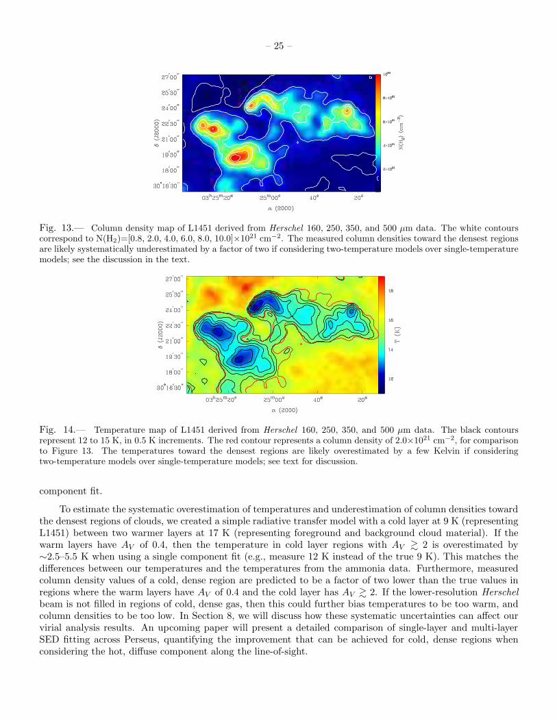
– 25 –

Fig. 13.— Column density map of L1451 derived from Herschel 160, 250, 350, and 500 µm data. The white contourscorrespond to N(H2)=[0.8, 2.0, 4.0, 6.0, 8.0, 10.0]×1021 cm−2. The measured column densities toward the densest regionsare likely systematically underestimated by a factor of two if considering two-temperature models over single-temperaturemodels; see the discussion in the text.

Fig. 14.— Temperature map of L1451 derived from Herschel 160, 250, 350, and 500 µm data. The black contoursrepresent 12 to 15 K, in 0.5 K increments. The red contour represents a column density of 2.0×1021 cm−2, for comparisonto Figure 13. The temperatures toward the densest regions are likely overestimated by a few Kelvin if consideringtwo-temperature models over single-temperature models; see text for discussion.

component fit.

To estimate the systematic overestimation of temperatures and underestimation of column densities towardthe densest regions of clouds, we created a simple radiative transfer model with a cold layer at 9 K (representingL1451) between two warmer layers at 17 K (representing foreground and background cloud material). If thewarm layers have AV of 0.4, then the temperature in cold layer regions with AV & 2 is overestimated by∼2.5–5.5 K when using a single component fit (e.g., measure 12 K instead of the true 9 K). This matches thedifferences between our temperatures and the temperatures from the ammonia data. Furthermore, measuredcolumn density values of a cold, dense region are predicted to be a factor of two lower than the true values inregions where the warm layers have AV of 0.4 and the cold layer has AV & 2. If the lower-resolution Herschel

beam is not filled in regions of cold, dense gas, then this could further bias temperatures to be too warm, andcolumn densities to be too low. In Section 8, we will discuss how these systematic uncertainties can affect ourvirial analysis results. An upcoming paper will present a detailed comparison of single-layer and multi-layerSED fitting across Perseus, quantifying the improvement that can be achieved for cold, dense regions whenconsidering the hot, diffuse component along the line-of-sight.

– 26 –

7.2. Dendrogram Analysis of Dust

The column density results in the previous section are angular resolution limited compared to our CLASSymaps, so it is difficult to estimate the mass within the smallest molecular structures we identified using thedendrogram analysis in Section 6. Therefore, we take the approach of first defining structures based on thedust data here, and then using the kinematic information within those structures to explore energy balance inthe next section.

We converted the NH2 column density map to an extinction map using a conversion factor of NH2/AV

= (1/2) × 1.87 × 1021 cm−2 mag−1 (Draine 2003). We then ran our non-binary dendrogram algorithm onthe extinction map to define dust structures in the field. We used an rms and branching step of 0.2 AV ,and required that local maxima peak at least 0.4 AV above the merge level to be considered a real leaf. Thealgorithm identified 8 leaves and 6 branches in the region where we have molecular line data.

The extinction map, with dendrogram-identified structures, is shown in Figure 15. Properties of thedendrogram structures are listed in Table 8, including their coordinate, size, weighted mean temperature andcolumn density, and total mass. The mean temperature and column density, and total mass of each structureconsiders all of the emission interior to the structure (e.g., branch 9 includes emission from branch 9 and leaves0 and 2). To calculate the total mass within each structure, we first converted the column density at each pixelto a solar mass unit as:

M(α, δ) = µH2mHNH2(α, δ)A, (1)

where µH2 is the molecular weight per hydrogen molecule (2.8), mH is the mass of a hydrogen atom, NH2(α, δ)is the column density at a pixel location, and A is the pixel area. As before, the assumed distance is 235 pc.We then totaled the mass enclosed within each structure. The mass of leaves ranges from 0.2 to 5.1 M⊙, andthe mass enclosed within branches ranges from 3.0 to 15.9 M⊙. The mass interior to the yellow and purplecontours in Figure 15 is 14.9 M⊙ and 12.4 M⊙, respectively.

Fig. 15.— Visual extinction map of L1451 (greyscale), as derived from the column density map in Figure 13. Thesolid black contour represents AV = 2, and the mean extinction within that contour is 3.8 mag with a 1.8 mag standarddeviation. Dendrogram-derived dust structure boundaries are shown with colored contours. The peak extinction is∼13 mag within structure 0.

– 27 –

Table 8. Dust Structure Properties

No. RA DEC Size 〈T〉 〈NH2〉 Mtot σ

tot,N2H+ σtot,HCN σtot,HCO+

(h:m:s) (◦:′:′′) (pc) (K) (1021 cm−2) (solar) (km s−1) (km s−1) (km s−1)(1) (2) (3) (4) (5) (6) (7) (8) (9) (10)

Leaves

0 03:25:13.3 +30:19:05.8 0.23 13.6 5.1 5.1 0.34 0.39 0.491 03:25:00.2 +30:21:22.1 0.08 14.4 2.8 0.2 ... 0.41 0.442 03:25:27.2 +30:21:43.6 0.17 13.2 5.0 3.1 0.27 0.29 0.403 03:24:35.5 +30:22:09.5 0.07 13.6 4.4 0.4 0.37 0.34 0.494 03:24:47.0 +30:23:11.2 0.14 13.9 4.0 1.4 ... 0.54 0.645 03:24:26.8 +30:22:47.7 0.17 13.9 4.6 2.0 0.28 0.44 0.536a 03:25:08.7 +30:24:09.5 0.07 12.2 7.2 0.5 0.25 0.25 0.337 03:25:01.5 +30:24:27.9 0.07 12.7 6.4 0.5 0.26 0.28 0.40

Branches

8 03:25:01.5 +30:24:12.9 0.21 13.7 4.1 3.0 0.33 0.33 0.429 03:25:17.8 +30:20:07.0 0.41 14.2 3.1 13.1 0.44 0.47 0.5410 03:24:29.2 +30:22:26.8 0.27 14.2 3.6 4.5 0.35 0.45 0.5711 03:24:54.2 +30:23:38.9 0.33 14.1 3.3 6.2 0.34 0.39 0.5112 03:24:43.1 +30:23:04.4 0.46 14.3 3.1 12.4 0.39 0.43 0.5413 03:25:17.1 +30:19:52.8 0.51 14.3 3.0 14.9 0.47 0.50 0.56

Note. — (4) Geometric mean of major and minor axis fit to structure (used as diameter of structure).(5) Weighted mean temperature within structure. (6) Weighted mean column density of H2 within

structure. (7) Total mass within structure. (8) N2H+ velocity dispersion calculated from integrated

spectrum across structure; see Section 8.2 for discussion. (9) HCN velocity dispersion calculated from

integrated spectrum across structure; see Section 8.2 for discussion. (10) HCO+ velocity dispersioncalculated from integrated spectrum across structure; see Section 8.2 for discussion. a L1451-mm islocated within this structure.

– 28 –

8. Discussion

The goal of this discussion section is to understand the state of star formation in L1451 using results andanalysis presented in previous sections. We selected L1451 as a CLASSy region because of its very low starformation activity. There are no confirmed protostar detections, and only one confirmed compact continuumcore. This is very different from the other CLASSy regions, which have many protostars and outflows. Wewanted to use L1451 to study the structure and kinematics of the densest regions of clouds before star formationactivity feeds back into the cloud.

We now explore the following questions. What column density threshold are we capturing with our spectralline observations, and do dendrogram-identified structures trace actual column density features that can informstructure formation in a young cloud? If so, will any structures go on to form stars? We address these questionsin this section by exploring the correspondence between molecular line and continuum emission, with a virialanalysis of L1451 structures, and by describing the similarities and differences between L1451-mm and L1451-west. We conclude with an analysis of the three-dimensional morphology of L1451 on the largest scales to seehow it compares to more evolved CLASSy regions.

8.1. Connecting molecular and column density structures

L1451 is the one CLASSy region with strong, widespread HCO+ and HCN that is not affected by outflowsand significant self-absorption. This enabled a dendrogram analysis of all three molecules in Section 6, insteadof just N2H

+, and lets us now compare the identified molecular structures to the column density structure ofL1451 presented in Section 7. Figures 16 and 17 have the dendrogram footprints of the lowest-level branches,and all the leaves, respectively, overplotted on column density structure derived from Herschel data. Wecombined the footprints of all the contoured emission in Figures 16 and 17 to create a mask for the columndensity map for determining how well the molecular emission captures material at different column densities.

Fig. 16.— Dendrogram lowest-level branch footprints for all molecules, overplotted on our extinction map that wasregridded to match the CLASSy pixel scale (beams for column density (36′′) and molecular (8′′) maps are in the lowerright). Red = HCO+, blue = HCN, and green = N2H

+. We label each branch with its dendrogram structure number,and branch properties can be examined in Tables 4–6.

Figure 18 shows cumulative distribution functions for column density in regions with and without lineemission (regions with line emission are defined as having at least a single molecular detection, while regionswithout line emission are defined as having no molecular detections). A threshold for star formation above

– 29 –

Fig. 17.— Dendrogram leaf footprints for all molecules, overplotted on our extinction map that was regridded to matchthe CLASSy pixel scale (beams for column density (36′′) and molecular (8′′) maps are in the lower right). Red = HCO+,blue = HCN, and green = N2H

+. We label a few examples with dendrogram structure numbers, and leaf properties canbe examined in Tables 4–6.

AV ∼ 8, or an H2 column density of 7.5 × 1021 cm−2, has been postulated based on the distribution of prestellarcores and protostars within the densest regions of molecular clouds (Johnstone et al. 2004; Hatchell et al. 2005;Andre et al. 2014, and references therein). Only 0.002% of dust regions without a molecular gas detection areabove the threshold column density if we take our derived column densities as correct. If our measured columndensities are uniformly underestimated by a factor of two from the true values, as was discussed in Section 7.1,still only 1% of dust regions without a molecular gas detection are above the threshold column density. 90%of the regions where we detect molecules are at column densities above 1.9 × 1021 cm−2, with a maximum of1.3 × 1022 cm−2, and minimum of 8.9 × 1020 cm−2. 90% of the regions where we do not detect moleculesare below 2.4 × 1021 cm−2, with a maximum of 7.8 × 1021 cm−2, and minimum of 3.6 × 1020 cm−2. Thisshows that spectral line observations using our suite of dense-gas tracer molecules are a great probe of the starforming material in young regions above the threshold for star formation and down to column densities of afew × 1021 cm−2.

This result of molecular emission capturing most of the cloud material near and above the threshold ofstar formation, combined with the result that the branches in Figure 16 are fragmenting to form the leavesin Figure 17 in a similar hierarchical fashion for each molecule (see Section 6.3), suggests that dendrogram-identified molecular structure is able to trace physical structure formation, despite some biases due to chemistryand extinction. This provides observational evidence that structure formation precedes star formation inmolecular clouds. Complex morphological structure in a turbulent cloud can be formed by turbulence-drivencascades from large-scale flows before the onset of star formation (Klessen & Hennebelle 2010, and referencetherein), and it can be produced from internally-driven turbulence from protostellar feedback (Carroll et al.2009; Federrath et al. 2014; Nakamura & Li 2014). Our result helps to disentangle externally and internallydriven structure, which it is important for demonstrating an observational case of complex, hierarchical densegas structure existing in a turbulent cloud at an epoch before internal feedback can impact the natal cloudenvironment.

– 30 –

0 2.0•1021 4.0•1021 6.0•1021 8.0•1021 1.0•1022 1.2•1022 1.4•1022

N(H2) (cm-2)

0.0

0.2

0.4

0.6

0.8

1.0

CD

F

0 2 4 6 8 10 12 14AV (mag)

detect gasdo not detect gas

Fig. 18.— Cumulative distribution functions for the areas of the L1451 column density map where we have detectedmolecular emission (solid curve), and the areas where we have not detected molecular emission (dashed curve). The solidvertical line marks the column density threshold for star formation (Andre et al. 2014, and references therein), while thedashed-dotted vertical line represents that threshold if our measured column densities are underestimated by a factor oftwo from the true column densities.

8.2. Virial Analysis of Structures

We next use a virial analysis to assess the stability of L1451 structures against collapse. We know one staris currently forming in L1451, based on the detection of compact 3 mm emission at L1451-mm. However, itis unknown if the majority of L1451 structures are dominated by gravitational potential energy and thereforeunstable against collapse, or rather dominated by internal pressure and therefore stable against collapse andpossibly confined by large external pressure. For the virial analysis, we use the dust results in combination withthe molecular data. In Section 7, we derived column densities and temperatures across L1451 at the angularresolution of the longest wavelength Herschel band (36′′). We also found dendrogram-identified dust structuresin the extinction map. In this section, we use that information for dust leaves along with CLASSy kinematicdata from Section 5 to assess the energy balance of several structures in L1451.

The virial theorem is useful for describing the stability of structures. There are several approaches for ap-plying the virial theorem to molecular cloud observations in the literature (e.g., Larson 1981; Bertoldi & McKee1992; McKee & Zweibel 1992; Ballesteros-Paredes 2006; Kauffmann et al. 2013). We follow the formalism ofBertoldi & McKee (1992) and Kauffmann et al. (2013), who define the observed virial parameter of an individ-ual structures as

αobs ≡5σ2

totR

GM(2)

where σtot, R, and M are the one-dimensional velocity dispersion (including thermal and non-thermal gasmotions), radius, and mass of the structure, respectively. Kauffmann et al. (2013) summarize that the criticalvalue of the virial parameter for a spherical structure not supported by magnetic pressure is α ≈ 2. Structureswith α ≪ 2 are supercritical and unstable against collapse unless they are supported by magnetic fields.Structures with α ≫ 2 are subcritical and stable against collapse—they should dissipate unless they are confinedby high external pressure. As discussed in Kauffmann et al. (2013), this critical value includes the effects ofdensity gradients within and outside of the structure, as well as surface pressure from the immediate surroundingmedium.

– 31 –

For the virial parameter definition in Equation 2, M is the mass of each source derived from our Herschelanalysis and is reported in Column 7 of Table 8. A major source of systematic uncertainty in the calculatedmass is the underestimate in the column density value derived from the Herschel SED fitting in Section 7.1.In Section 7.1, we discussed how using a single temperature model (ignoring the warmer foreground andbackground component surrounding the colder L1451 region) for fitting the Herschel SEDs leads to estimatedcolumn densities that are about a factor of two lower than the true column densities. If the measured columndensities are a factor of two lower than the true column densities, this directly leads to a mass underestimate bya factor of two and a virial parameter overestimate by a factor of two. Work has been done on the galactic scaleto estimate dust mass underestimation due to poor spatial resolution and temperature mixing in Herschel data.For example, Galliano et al. (2011) found that Herschel-derived dust masses can be ∼50% underestimated inthe Large Magellanic Cloud (LMC). Even though our observations have much higher spatial resolution thanobservations of the LMC, this is a useful comparison since the warm-cold temperature contrast in local cloudslike L1451 may be more extreme than on galactic scales. For core scales, Shetty et al. (2009) demonstrated thattemperature variations along the line-of-sight will lead to inaccurate measurements of dust properties from SEDfitting. We will consider the likely systematic underestimation of mass from our SED fitting in the discussionof results below.

The radius of each structure, R, in the virial parameter definition is half of the size reported in Column 4of Table 8. The one-dimensional velocity dispersion of each structure, σtot, in the virial parameter definitionincludes thermal and non-thermal support against collapse. The thermal component of the velocity dispersionwas calculated as:

σth =

√

kT

µmH

, (3)

where T is the mean temperature of the dust within the structure, µ is the mean molecular weight (2.33), andmH is the hydrogen atomic mass. The non-thermal component of the velocity dispersion was calculated foreach molecular tracer separately, as:

σnth,tracer =√

σ2obs,tracer − σ2

th,tracer (4)

where σ2obs,tracer is the observed velocity dispersion of the molecular emission within the structure, and σth,tracer

is the thermal velocity dispersion of the molecule at the mean temperature found within the structure:

σth,tracer =

√

kT

µtracermH

. (5)

We determined σ2obs,tracer by masking the CLASSy molecular data cubes using the boundaries of each dust

structure, generating an integrated spectrum for each molecule, and fitting for the velocity dispersion of thatintegrated spectrum. The final σtotal,tracer value was then calculated as:

σtot,tracer =√

σ2th

+ σ2nth,tracer

(6)

and is reported in Columns 8, 9, and 10 of Table 8 for N2H+, HCN, and HCO+, respectively. The temperature

overestimate from the single-temperature Herschel SED fitting discussed in Section 7.1 systematically increasesthe thermal component of the internal velocity dispersion of each structure, thereby increasing the dispersiveterm used to calculate α. The temperature error is less significant than the factor of two column densityerror discussed above, but still contributes a ∼7% systematic increase in the virial parameter if the measuredtemperature is overestimated by 2.5 K from the true value.

Virial parameters for each dust leaf structure are reported in Table 9, with unique values for each moleculartracer resulting from different velocity dispersions between the tracers. For each tracer, we first report the

– 32 –

measured virial parameter using the masses derived from the Herschel SED fitting, and then report a valuereduced by a factor of two to account for the likely systematic underestimation of the fitted column densityvalues discussed above.

Two things are clear from the α values in Table 9. First, the α values typically vary by a factor oftwo between tracers, with N2H

+ and HCO+ data giving the lowest and highest virial parameter, respectively.This trend with molecular tracer is not surprising, since it connects to the differences in spatial extent andkinematics between molecular emission discussed in Sections 4 and 5. The HCO+ traces the most spatiallyextended emission on the plane of the sky, implying it is tracing the most extended emission along the line-of-sight if the two spatial directions are correlated. This implication is strongly supported by HCO+ havingthe largest line-of-sight velocity dispersions. Since the virial parameter scales as the square of the velocitydispersion of each molecule, the larger HCO+ velocity dispersion leads to the larger virial parameter. Thisshows that the choice of kinematic tracer has large impact on the interpretation of a given structure.

Second, all virial parameter values are greater than two if we use the masses derived from the single-temperature model of Herschel SED fitting. If we assume that the mass is underestimated by a factor of twoand the virial parameter is overestimated by a factor of two (ignoring the systematic temperature uncertaintyalso increasing the virial parameter), then some of the structures have virial parameters near or less than thecritical value of 2 for instability against collapse. Structures 1, 3, 4, and 7 have α above two regardless of themolecular tracer used or assumption of mass. These structures have the weakest dense gas emission in thefield and/or appear the least centrally condensed in the column density maps, so it is reasonable that theyappear to be the least unstable against collapse. Structures 0, 2, 5, and 6 have α near or below two, appearcentrally condensed in the column density map, and have strong molecular emission in the line maps. Structure0 contains Per Bolo 4, structure 2 contains Per Bolo 6, structure 5 contains L1451-west, and structure 6 containsL1451-mm. These results together support these structures (or at least the central parts of these structures)being unstable against collapse, and the L1451 region as a whole being at the onset of forming a few protostars.

We will extend this type of virial analysis in upcoming work to compare virial parameters across CLASSyregions. This way, even if there are systematic and statistical uncertainties, all structures will have beenobserved and analyzed in the same way, making a relative comparison of virial parameters across cloud regionsat different stages of evolution possible.

– 33 –

Table 9. Virial Parameters

α (N2H+) α (HCN) α (HCO+)

No. 1-temp 2-tempa 1-temp 2-tempa 1-temp 2-tempa

(1) (2) (3) (4) (5) (6) (7)0 3.0 1.5 4.0 2.0 6.1 3.11 ... ... 28.5 14.3 32.9 16.52 2.3 1.2 2.8 1.4 5.2 2.63 15.3 7.7 13.1 6.6 26.0 13.04 ... ... 17.5 8.8 24.8 12.45 3.8 1.9 9.3 4.7 13.5 6.86b 4.4 2.2 4.5 2.3 7.9 4.07 6.2 3.1 6.8 3.4 14.0 7.0

Note. — (1) Leaf number from Table 8. (2) Virial parameter calculated usingEquation 2 with the N2H

+ velocity dispersion and mass derived from Herschel

single-temperature SED fitting. (3) Column 2, corrected by a factor of two toaccount for the likely underestimation of column density (and therefore mass)from single-temperature SED fitting discussed in text. (4) Same as Column 2,but using the HCN velocity dispersion. (5) Same as Column 3, but using theHCN velocity dispersion. (6) Same as Column 2, but using the HCO+ velocitydispersion. (7) Same as Column 3, but using the HCO+ velocity dispersion.aWe are not formally using a two-temperature model to fit the Herschel SEDs,but are applying a correction factor that estimates the likely effect of using sucha model. bL1451-mm is located within this structure.

– 34 –

8.3. Closer Look at L1451-mm and L1451-west

In this section, we explore the properties of the two centrally condensed, roughly spherical cores in L1451.One is L1451-mm, which we know is a compact object containing a YSO or a FHSC (Pineda et al. 2011).The other is L1451-west, which has been discovered with these observations. We summarize the morphologyand kinematics of L1451-mm below, and then describe the properties of L1451-west and how they compare toL1451-mm.

The top row of Figure 19 shows molecular and continuum features of L1451-mm. L1451-mm is the onlyconfirmed compact continuum core in L1451, and all molecules trace strong emission near, and surrounding itslocation. All molecules peak in integrated emission at a location slightly offset from the L1451-mm compactcontinuum core. The molecular emission that surrounds the core is more concentrated for N2H

+, and morewidespread for HCN and HCO+. The N2H

+ centroid velocity field shows a gradient across the core, whichPineda et al. (2011) modeled as a rotating and infalling envelope using slightly higher angular resolution (5′′)data; we measure a gradient of about 6 km s−1 pc−1 through the peak of integrated emission at a positionangle of 120 deg east of north (see white line in the top row panels of Figure 19). The velocity dispersion fieldis narrowest around the edges of the core with minima ∼0.07 km s−1, and it shows an increase toward thecore location, with a peak ∼0.2 km s−1. See Pineda et al. (2011) for detailed discussion and modeling of thepossibility that L1451-mm is a dense core with a central YSO and disk, or a dense core with a central FHSC.

Fig. 19.— The top and bottom rows show properties of L1451-mm and L1451-west, respectively. From left-to-right,the panels are: N2H

+, HCN, and HCO+ integrated intensity (Jy beam−1 km s−1), N2H+ centroid velocity (km s−1),

and N2H+ velocity dispersion (km s−1). The kinematic maps of each source are on the same color scale. The velocity

dispersion is expressed as Gaussian σ (FWHM/2.355 in km s−1). The green 0.0039 mJy beam−1 contour represents ourL1451-mm compact continuum detection. The red contours are used to accentuate specific features in the greyscale maps.The white lines represent the direction of the measured velocity gradient through L1451-mm.

The bottom row of Figure 19 shows molecular and continuum features of L1451-west. The N2H+ integrated

intensity map does not have a single peak of integrated emission at the center of the structure. Instead, thereare two peaks in the southern half of the source ∼2.5 Jy beam−1 km s−1, and one peak in the northern halfof the source ∼2.4 Jy beam−1 km s−1 (the red contours in the bottom-left panel of Figure 19 represent 1.1–2.5 Jy beam−1 km s−1 in 0.2 Jy beam−1 km s−1 increments). The source is considerably weaker in HCN, andnot detected in HCO+. This apparent lower-abundance of HCO+ may indicate that this might be a very cold,dense region of L1451, where CO is depleted. If CO is frozen out onto dust grains, then it is not able to destroy

– 35 –

N2H+, and N2H

+ remains abundant. Likewise, if CO is frozen out, it is not available to create HCO+ throughcollisions with H3

+ (Prasad & Huntress 1980). Our temperature map in Figure 14 does not suggest that dustaround L1451-west is significantly colder than L1451-mm, but higher-resolution continuum observations withmodeling to remove any warm component could reveal differences in the two sources that are not resolvablewith the current data. It is also possible that the HCO+ (J = 1 → 0) photons are being absorbed by HCO+

molecules in lower-density foreground gas; observations of higher-J transitions are needed to test this.

The N2H+ centroid velocity field of L1451-west shows a relatively complex structure compared with L1451-

mm, with higher velocity emission in the southern and northeastern sections of the core, and lower velocityemission toward the center and west of the core. The velocity dispersion field of L1451-west is narrowest aroundthe edges of the core with minima ∼0.07 km s−1, and it peaks near ∼0.2 km s−1 at the location of lowest velocityemission in the central part of the source. It is possible that infall is producing the increased velocity dispersion,in addition to any undetected outflows and/or unresolved disk rotation from source center. Infall would broadenthe molecular emission toward the core center, with the blueshifted emission being brighter than the redshiftedemission if the N2H

+ emission is optically thick. This could explain why the peak of velocity dispersion is atthe location with the bluest centroid velocity. The signal-to-noise of the detectable HCN spectra are too low tolook for evidence of infall motions, so this needs to be followed up with deeper observations of optically thickand thin lines.

There is no compact continuum emission detected toward L1451-west. The 3σ flux density limit for apoint source (.3′′ = 700 AU) in our observations is 3.9 mJy, corresponding to a mass limit of 0.08 M⊙ for theconversion from mJy to M⊙ discussed in Paper I. We use the location of peak velocity dispersion as a proxy forthe location of a compact continuum core, if it exists; this peak is offset from the peak in the Herschel-derivedcolumn density map by about 16′′.

We estimated the size and physical density of L1451-mm and L1451-west for a more detailed comparison.To determine the size, we used the MIRIAD imfit routine to fit a two-dimensional Gaussian to the N2H

+

integrated intensity map. The geometric means of the major and minor axes are 37′′ and 32′′ for L1451-mmand L1451-west, respectively. To determine the maximum physical density, we took the peak column density ofeach source within the fitted Gaussian, and assumed their depth was the same extent as their geometric meanacross the plane of the sky. For both sources, the physical density is 7–8× 104 cm−3 in the 8′′ beam. Thisdensity is sensible, considering that we observe N2H

+ and HCN (J = 1 → 0) in L1451, which are moleculartransitions with effective excitation densities on the order of 105 cm−3.

We also compared the mass within 4200 AU (18′′ at d=235 pc) to the intrinsic radius at 70% of peakintensity, following the analysis of starless cores presented in Kauffmann et al. (2008). We measured the massusing the Herschel data, and got 0.22 and 0.23 M⊙ for L1451-mm and L1451-west, respectively. We measuredthe radius using the N2H

+ integrated intensity, since the dust data is not as well resolved to derive accurateradius measurements. L1451-mm measured 8′′, and L1451-west measured 12′′ at 70% of the peak intensity.Compared to the sample of starless cores in Kauffmann et al. (2008), L1451-mm is more centrally dense thanmost starless objects, while L1451-west is near the upper limit of central density seen in starless objects.

All of these observational results point to L1451-west being similar to, but slightly less evolved than,L1451-mm, yet more evolved than a prestellar core. Although deep continuum and spectral line observationswill be needed to determine the true nature of these sources, they are some of the best evidence that L1451 isa region that is just starting to form its first stars.

8.4. Three-Dimensional Morphology of L1451

Comparing the projected size of cloud structure to its depth along the line-of-sight gives a better under-standing of the three-dimensional geometry of a region where stars are forming (e.g., a region that is primarily

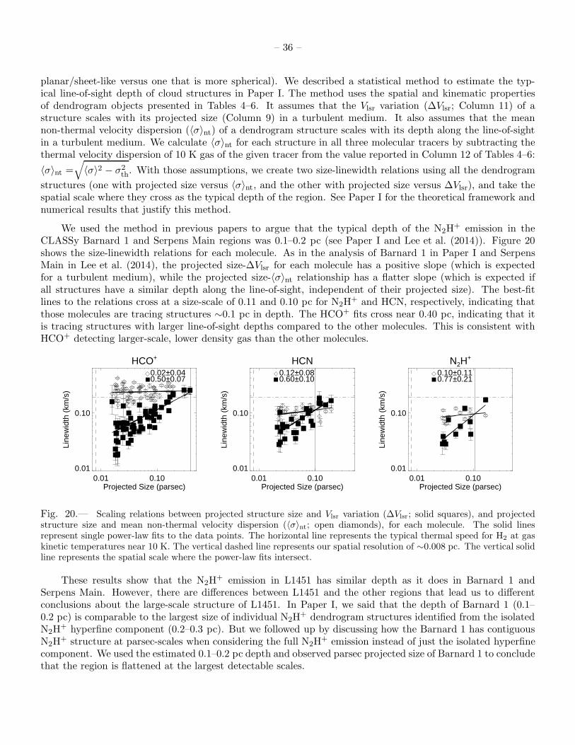
– 36 –

planar/sheet-like versus one that is more spherical). We described a statistical method to estimate the typ-ical line-of-sight depth of cloud structures in Paper I. The method uses the spatial and kinematic propertiesof dendrogram objects presented in Tables 4–6. It assumes that the Vlsr variation (∆Vlsr; Column 11) of astructure scales with its projected size (Column 9) in a turbulent medium. It also assumes that the meannon-thermal velocity dispersion (〈σ〉nt) of a dendrogram structure scales with its depth along the line-of-sightin a turbulent medium. We calculate 〈σ〉nt for each structure in all three molecular tracers by subtracting thethermal velocity dispersion of 10 K gas of the given tracer from the value reported in Column 12 of Tables 4–6:

〈σ〉nt =√

〈σ〉2 − σ2th. With those assumptions, we create two size-linewidth relations using all the dendrogram

structures (one with projected size versus 〈σ〉nt, and the other with projected size versus ∆Vlsr), and take thespatial scale where they cross as the typical depth of the region. See Paper I for the theoretical framework andnumerical results that justify this method.

We used the method in previous papers to argue that the typical depth of the N2H+ emission in the

CLASSy Barnard 1 and Serpens Main regions was 0.1–0.2 pc (see Paper I and Lee et al. (2014)). Figure 20shows the size-linewidth relations for each molecule. As in the analysis of Barnard 1 in Paper I and SerpensMain in Lee et al. (2014), the projected size-∆Vlsr for each molecule has a positive slope (which is expectedfor a turbulent medium), while the projected size-〈σ〉nt relationship has a flatter slope (which is expected ifall structures have a similar depth along the line-of-sight, independent of their projected size). The best-fitlines to the relations cross at a size-scale of 0.11 and 0.10 pc for N2H

+ and HCN, respectively, indicating thatthose molecules are tracing structures ∼0.1 pc in depth. The HCO+ fits cross near 0.40 pc, indicating that itis tracing structures with larger line-of-sight depths compared to the other molecules. This is consistent withHCO+ detecting larger-scale, lower density gas than the other molecules.

HCO+

0.01 0.10Projected Size (parsec)

0.01

0.10

Line

wid

th (

km/s

)

0.02±0.040.50±0.07

HCN

0.01 0.10Projected Size (parsec)

0.01

0.10

Line

wid

th (

km/s

)

0.12±0.080.60±0.10

N2H+

0.01 0.10Projected Size (parsec)

0.01

0.10

Line

wid

th (

km/s

)0.10±0.110.77±0.21

Fig. 20.— Scaling relations between projected structure size and Vlsr variation (∆Vlsr; solid squares), and projectedstructure size and mean non-thermal velocity dispersion (〈σ〉nt; open diamonds), for each molecule. The solid linesrepresent single power-law fits to the data points. The horizontal line represents the typical thermal speed for H2 at gaskinetic temperatures near 10 K. The vertical dashed line represents our spatial resolution of ∼0.008 pc. The vertical solidline represents the spatial scale where the power-law fits intersect.

These results show that the N2H+ emission in L1451 has similar depth as it does in Barnard 1 and

Serpens Main. However, there are differences between L1451 and the other regions that lead us to differentconclusions about the large-scale structure of L1451. In Paper I, we said that the depth of Barnard 1 (0.1–0.2 pc) is comparable to the largest size of individual N2H

+ dendrogram structures identified from the isolatedN2H

+ hyperfine component (0.2–0.3 pc). But we followed up by discussing how the Barnard 1 has contiguousN2H

+ structure at parsec-scales when considering the full N2H+ emission instead of just the isolated hyperfine

component. We used the estimated 0.1–0.2 pc depth and observed parsec projected size of Barnard 1 to concludethat the region is flattened at the largest detectable scales.

– 37 –

In projection, the full N2H+ emission, sub-millimeter continuum emission, and other molecular emission

from L1451 region does not appear to have contiguous structure across parsec scales like all other CLASSyregions. Instead, the emission is concentrated in a few major features, sub-parsec in size, that were identifiedin Section 4. Because of this, we argue that the L1451 is not a flattened, sheet-like region of dense gas anddust at parsec-scales with connected substructure. In N2H

+, it appears more like a loose collection of denseconcentrations that are ∼0.2 pc projected on the sky and ∼0.1 pc deep.

The physical density of the regions of L1451 with N2H+ emission can be estimated from the cloud depth

and column density. For a 0.1 pc depth of N2H+ emission and a mean N(H2) of 6 × 1021 cm−2 measured from

the Herschel data, the derived physical density is 2 × 104 cm−3 in the regions of L1451 with N2H+ emission.

It is possible to excite N2H+ at a range of physical densities, where the range depends on the molecular

column density (and thus relative abundance of N2H+ to H2), the gas kinetic temperature, and the linewidth

of emission. Using the RADEX program (van der Tak et al. 2007), we find that N2H+ (J = 1 → 0) can reach

1 K brightness temperatures with a physical density of 2.7 × 104 cm−3 if the gas kinetic temperature is 12 K,the molecular column density of N2H

+ is 6 × 1012 cm−2, and the linewidth of emission is 0.3 km s−1. Thisphysical density is essentially the same as derived from our depth and column density measurements, providinga consistency check to our measurements.

We can compare the typical depth of the molecular emission to the projected size of the largest-scalestructures of each molecule in Figure 16 to infer the three-dimensional morphology of the individual molecularstructures. The projected size of N2H

+ structure 21 (lowest level branch of Features A) is ∼0.17 pc, structure18 (lowest level branch of Features C) is ∼0.09 pc, and structure 17 (lowest level branch of Features B) is∼0.17 pc. For a typical N2H

+ depth of 0.11 pc, these structures have axis ratios of 1.5:1 and 0.8:1, with a meanof 1.3:1. The projected size of HCN structure 45 (lowest level branch of Feature A) is ∼0.24 pc, structure 43(lowest level branch of Feature C) is ∼0.17 pc, and structure 40 (lowest level branch of Feature B) is ∼0.19 pc.For a typical HCN depth of 0.10 pc, these structures have axis ratios between 2.4:1 and 1.7:1, with a mean axisratio of 2.0:1. The projected size of HCO+ structure 111 (lowest level branch connecting Features A and C) is∼0.43 pc, and structure 112 (lowest level branch connecting Features B, H, F, G, E, and I) is ∼0.46 pc. Forour derived typical HCO+ depth of 0.40 pc, these structures have axis ratios of 1.1:1 and 1.2:1.

With axis ratios between 0.8:1 and 2.4:1 for individual structures that do not connect at larger scales, theseresults support the L1451 region being composed of discrete, high-density structures that are approximatedas ellipsoids. In addition to not having contiguous, flattened structure at parsec scales like the other CLASSyregions studied to-date (Serpens Main and Barnard 1), none of the large-scale structures of L1451 appear tohave clear filamentary substructure like was the case in all other CLASSy regions. These results differentiateL1451 from the other regions in a way beyond the lack of protostars and outflows.

If L1451 is not a flattened, sheet-like region at parsec-scales, if it does not have prominent filamentarystructure, and if it has less active star formation than the other CLASSy regions, then it is natural to speculatewhat caused these differences. A cloud complex, like Perseus, that spans tens of parsecs will have differentturbulent energies in different parts of the cloud. Simulations of turbulence-driven star formation with super-sonic turbulence (e.g., Federrath & Klessen 2012) show that star formation within several-parsec scale cloudsis clustered in regions where material has been compressed to high densities, leaving voids of star formationin other parts of the cloud. We speculate that the L1451 region of Perseus may not have been compressedas strongly by supersonic turbulence to form an overdense sheet-like structure at parsec-scales like may havehappened several parsecs away near the cloud regions that became Barnard 1 and NGC 1333. Without acomparable push to high-density that other more active regions of Perseus got, the L1451 region may havebeen predisposed to forming fewer stars.

– 38 –

9. Summary of L1451 Results

We presented observations and analysis of the L1451 region of the CARMA Large Area Star FormationSurvey. We summarize the key findings below.

1. Only one compact continuum source is detected at 3 mm, down to a 3σ limit of 3.9 mJy beam−1 (0.08 M⊙

limit) in a 9.2′′ × 6.6′′ beam. The detected source is L1451-mm, which has previously been identified asa FHSC candidate.

2. We detect widespread HCO+, HCN, and N2H+ (J = 1 → 0) emission in L1451. The HCO+ emission

covers the largest area of the cloud, which we attribute to HCO+ tracing lower-density material than theother molecules. HCN emission morphology is nearly identical to HCO+, although it is weaker and lessspatially extended in most regions. We detect no molecular outflows from HCO+ or HCN. The N2H

+

emission appears the most spatially compact, and reveals a newly identified compact core, which we callL1451-west.

3. All molecules trace gas at similar systemic velocities, but the velocity dispersion of the HCO+ emissionis significantly larger than that of HCN or N2H

+: mean dispersions are 0.29, 0.16, and 0.12 km s−1,respectively. This is likely due to HCO+ tracing lower-density gas at larger scales than the other twomolecules; in a turbulent medium, there is more power on larger scales, which will produce larger velocitydispersions.

4. We derive column density and temperature maps from Herschel observations at 160, 250, 350, and 500 µm.The values were derived using modified blackbody spectrum fits to the data, and column densities agreeto within 5% of Planck results when compared at the same angular resolution. The temperatures towardthe densest regions are ∼2–3 K warmer than kinetic temperatures derived from single-pointing ammoniaobservations toward dense cores. We attribute this difference to a limitation of using a single-componentfit when modeling SEDs from cold, dense regions of molecular clouds. A simple multi-layer model showsthat having warm, 17 K foreground and background emission surrounding cold, 9 K cloud emission, cancause temperatures to be overestimated by a few K, and column densities to be underestimated by afactor of two.

5. The structure of the star-forming material in L1451 that is traced by the cumulative molecular emission wedetect with CLASSy is very similar to the column density structure we derived from Herschel observations.All of the cloud locations that are above the AV ∼ 8 threshold for star formation are detected in densegas, and 90% of the molecular emission is at column densities above 1.9 × 1021 cm−2. This shows thathigh-resolution observations of this suite of spectral lines over large areas of molecular clouds are anexcellent probe of the structure and kinematics of star forming material in young regions.

6. We use our non-binary dendrogram algorithm to identify dense gas structures in the HCO+, HCN, andN2H

+ data cubes. The number of identified leaf and branch dendrogram structures decreases from HCO+

to HCN to N2H+, providing an apparently wide range of hierarchical complexity in the different tracers.

However, a uniform comparison of tree statistics that accounts for differences in the noise-level of each datacube shows that all tracers are identifying structures that are fragmenting in a similar way. The differencesin dendrogram branching levels and number of structures between tracers are likely due to differences indensity sensitivity of the different tracers. We show that tree statistics of the gas structure surroundingL1451-mm (a confirmed young protostar or FHSC) is very similar to that of the gas surrounding Per Bolo 6(a single-dish continuum detection), and argue this is an indication that star formation is proceeding ina similar fashion in both regions, with Per Bolo 6 a likely site of future star formation.

– 39 –

7. A virial analysis of dust structures identified in our Herschel-derived extinction map of L1451 resulted inall structures being stable against collapse when using the masses derived from single-temperature Her-

schel SED fitting and velocity dispersion from any CLASSy molecular tracer. However, we discussed howthe virial parameter is likely overestimated by about a factor of two from the systematic underestimationof column densities from the simplistic single-temperature SED fitting. Also, the virial parameter of agiven structure is strongly dependent on the molecular tracer used to estimate its kinetic energy; N2H

+

and HCO+ resulted in the lowest and highest virial parameters, respectively, with typical differences ofabout a factor of two. The dust structures that appear most centrally condensed in the dust maps arenear or below the critical value for instability when considering the systematic uncertainty to the massand using the N2H

+ or HCN velocity dispersion.

8. We detect two strong, centrally condensed N2H+ structures: L1451-mm, and a newly identified source

that we label L1451-west. L1451-mm was characterized by Pineda et al. (2011) as a FHSC candidate oryoung protostar. Our data shows that L1451-west is similar to, but likely younger than L1451-mm. It hasstrong emission from N2H

+ but appears depleted in HCO+, unlike L1451-mm which has strong emissionfrom both molecules. Both sources show N2H

+ velocity dispersions peaking at the core center. L1451-west is less centrally condensed than L1451-mm, but more centrally condensed that the typical prestellarcore; this indicates that L1451-west is likely at an evolutionary state between the typical prestellar coreand a FHSC or young protostar. Follow-up observations will determine if L1451-west is a viable FHSCcandidate.

9. We use our size-linewidth analysis first presented in Paper I to estimate the typical line-of-sight depth ofdense gas structures in L1451. Typical inferred line-of-sight depths for HCO+ structures are 0.40 pc, andfor HCN and N2H

+ structures are ∼0.10 pc. These depths are found to be within a factor of two of theprojected sizes of gas structures, showing that the three-dimensional dense gas morphology in L1451 isrelatively ellipsoidal at the largest detectable scales when compared to the more evolved CLASSy regionsthat appear flattened/sheet-like at the largest scales.

Overall, these observations support the creation of complex, hierarchical dense gas structure in molecularclouds without internal feedback from protostars. We cannot say that individual structures within L1451 aredefinitively gravitationally bound based on our analysis, but that several structures are consistent with beingunstable to collapse within the uncertainties in the data; we also know at least one star is forming in the regionbased on compact continuum detections. The velocities in these structures are larger than pure thermal andrange from subsonic gas motions on the smallest scales (as traced by N2H

+) to slightly supersonic gas motionson the largest scales (as traced by HCO+); this supports external supersonic turbulence on even larger scalesthan those traced by HCO+ being the driver of the first structure within the densest regions of molecular cloudcomplexes; those structures then become the dense, fertile grounds for the future formation of stars.

The science-ready spectral line data cubes for L1451 are hosted at our project website:http://carma.astro.umd.edu/classy. We welcome the community to make use of the data.

The authors would like to thank the referee for encouraging critiques that improved the paper, and allmembers of the CARMA staff that made these observations possible. CLASSy was supported by AST-1139990(University of Maryland) and AST-1139950 (University of Illinois). Support for CARMA construction wasderived from the Gordon and Betty Moore Foundation, the Kenneth T. and Eileen L. Norris Foundation,the James S. McDonnell Foundation, the Associates of the California Institute of Technology, the Universityof Chicago, the states of Illinois, California, and Maryland, and the National Science Foundation. OngoingCARMA development and operations are supported by the National Science Foundation under a cooperativeagreement, and by the CARMA partner universities.

Facility: CARMA

– 40 –

REFERENCES

Andre, P., Di Francesco, J., Ward-Thompson, D., et al. 2014, Protostars and Planets VI, 27

Aniano, G., Draine, B. T., Gordon, K. D., & Sandstrom, K. 2011, PASP, 123, 1218

Ballesteros-Paredes, J. 2006, MNRAS, 372, 443

Beckwith, S. V. W., & Sargent, A. I. 1991, ApJ, 381, 250

Bergin, E. A., & Tafalla, M. 2007, ARA&A, 45, 339

Bertoldi, F., & McKee, C. F. 1992, ApJ, 395, 140

Carroll, J. J., Frank, A., Blackman, E. G., Cunningham, A. J., & Quillen, A. C. 2009, ApJ, 695, 1376

Crutcher, R. M. 2012, ARA&A, 50, 29

di Francesco, J., Evans, II, N. J., Caselli, P., et al. 2007, Protostars and Planets V, 17

Draine, B. T. 2003, ARA&A, 41, 241

Elmegreen, B. G., & Scalo, J. 2004, ARA&A, 42, 211

Enoch, M. L., Evans, II, N. J., Sargent, A. I., et al. 2008, ApJ, 684, 1240

Enoch, M. L., Young, K. E., Glenn, J., et al. 2006, ApJ, 638, 293

Evans, II, N. J. 1999, ARA&A, 37, 311

Evans, II, N. J., Dunham, M. M., Jørgensen, J. K., et al. 2009, ApJS, 181, 321

Federrath, C., & Klessen, R. S. 2012, ApJ, 761, 156

Federrath, C., Schron, M., Banerjee, R., & Klessen, R. S. 2014, ApJ, 790, 128

Fernandez-Lopez, M., Arce, H. G., Looney, L., et al. 2014, ApJ, 790, L19

Galliano, F., Hony, S., Bernard, J.-P., et al. 2011, A&A, 536, A88

Hatchell, J., Richer, J. S., Fuller, G. A., et al. 2005, A&A, 440, 151

Johnstone, D., Di Francesco, J., & Kirk, H. 2004, ApJ, 611, L45

Jørgensen, J. K., Johnstone, D., Kirk, H., et al. 2008, ApJ, 683, 822

Kauffmann, J., Bertoldi, F., Bourke, T. L., Evans, II, N. J., & Lee, C. W. 2008, A&A, 487, 993

Kauffmann, J., Pillai, T., & Goldsmith, P. F. 2013, ApJ, 779, 185

Kirk, H., Johnstone, D., & Di Francesco, J. 2006, ApJ, 646, 1009

Klessen, R. S., & Hennebelle, P. 2010, A&A, 520, A17

Larson, R. B. 1981, MNRAS, 194, 809

Lee, K. I., Fernandez-Lopez, M., Storm, S., et al. 2014, ApJ, 797, 76

McKee, C. F., & Ostriker, E. C. 2007, ARA&A, 45, 565

– 41 –

McKee, C. F., & Zweibel, E. G. 1992, ApJ, 399, 551

Meisner, A. M., & Finkbeiner, D. P. 2015, ApJ, 798, 88

Nakamura, F., & Li, Z.-Y. 2007, ApJ, 662, 395

—. 2014, 783, 115

Pineda, J. E., Arce, H. G., Schnee, S., et al. 2011, ApJ, 743, 201

Planck Collaboration, Abergel, A., Ade, P. A. R., et al. 2014, A&A, 571, A11

Prasad, S. S., & Huntress, Jr., W. T. 1980, ApJS, 43, 1

Rosolowsky, E. W., Pineda, J. E., Foster, J. B., et al. 2008a, ApJS, 175, 509

Rosolowsky, E. W., Pineda, J. E., Kauffmann, J., & Goodman, A. A. 2008b, ApJ, 679, 1338

Sadavoy, S. I., di Francesco, J., Andre, P., et al. 2012, A&A, 540, A10

Sault, R. J., Teuben, P. J., & Wright, M. C. H. 1995, in Astronomical Society of the Pacific Conference Series,Vol. 77, Astronomical Data Analysis Software and Systems IV, ed. R. A. Shaw, H. E. Payne, & J. J. E.Hayes, 433

Shetty, R., Kauffmann, J., Schnee, S., Goodman, A. A., & Ercolano, B. 2009, ApJ, 696, 2234

Shirley, Y. L. 2015, PASP, 127, 299

Storm, S., Mundy, L. G., Fernandez-Lopez, M., et al. 2014, ApJ, 794, 165

van der Tak, F. F. S., Black, J. H., Schoier, F. L., Jansen, D. J., & van Dishoeck, E. F. 2007, A&A, 468, 627

Williams, J. P., de Geus, E. J., & Blitz, L. 1994, ApJ, 428, 693

A. Noise Dependence of Dendrogram Structure and Statistics

In Paper I, we analyzed a single non-binary dendrogram from the position-position-velocity (PPV) cube ofthe isolated hyperfine component of N2H

+ in Barnard 1. In this paper, we analyzed the non-binary dendrogramsfrom the PPV cubes of the strongest hyperfine components of N2H

+ and HCN, and the single component ofHCO+ in L1451. There was a noise difference of 15% between those cubes, and the goal of this section isto establish how we can compare dendrogram structure and statistics of data with different noise-levels. Wewill argue that the key for a proper comparison is to construct the dendrograms using absolute, physical units(as opposed to units based on the sensitivity of an individual data set) for certain dendrogram algorithmparameters, including the parameters for: 1) the minimum height for a local maximum to peak above the levelwhere it merges with adjacent local maxima to be considered a real leaf (minheight), and 2) the minimumallowed branching step height between adjacent levels in the dendrogram (stepsize).

We will demonstrate those points using two integrated intensity maps of Barnard 14 that have similarsignal but different noise, created from different hyperfine components in the N2H

+ PPV cube presented in

This preprint was prepared with the AAS LATEX macros v5.2.

4We use Barnard 1 instead of L1451 for demonstration in this appendix because Barnard 1 was the first CLASSy region analyzedand used to test the dendrogram analysis methods.

– 42 –

Paper I. The N2H+ (J = 1 → 0) transition is split into seven resolvable hyperfine components, which have

effectively the same velocity dispersion and excitation condition but different peak intensity. We can integrateover different combinations of hyperfine components to create moment maps with different signal-to-noise ratio(SNR). Specifically, we integrate over all seven hyperfine components to create a “full-velocity component”integrated intensity map (referred to as the FVC map later in the section), and over the isolated velocitycomponent to make the “lowest-velocity component” integrated intensity map (referred to as the LVC maplater in the section). The LVC map has lower signal than the FVC map, but also lower noise (σLV C) inemission-free regions compared to the FVC map (σFV C), since noise scales as

√Nσ, where N is the number of

channels, and σ is the noise in a single channel.

The questions we want to answer hinge on how to consistently analyze dendrogram structure and statisticswhen we change the noise in a map while keeping the signal the same. Therefore, we normalize the FVC mapto have the same signal as the LVC map in regions where the LVC map has emission greater than 6σLV C . Inregions less than 6σLV C in the LVC map, we scale the FVC map down by a factor of 7, which is the meannormalization factor in regions of strong signal. We then calculate the rms of the normalized FVC map (referredto as the NFVC map later in the section), σNFV C , which is 0.03 Jy beam−1 km s−1, compared to σLV C of0.09 Jy beam−1 km s−1. The result is a NFVC map with similar signal to the LVC map with three times lowernoise; this is the scenario we want to test our dendrogram algorithm on.

We ran our non-binary dendrogram algorithm on the Barnard 1 versions of these two maps in two differentways. First, we allowed each dendrogram to have a stepsize and minheight based on the rms of each map,meaning stepsize = 1σNFV C and minheight = 2σNFV C for the NFVC map, and stepsize = 1σLV C andminheight = 2σLV C for the LVC map. Second, we forced each dendrogram to have the same stepsize andminheight based on the noisier map, meaning stepsize = 1σLV C and minheight = 2σLV C for both maps.Using absolute units across maps as in this second case could be beneficial because absolute units are linked withphysical properties of a cloud, while noise units are linked with the properties of the individual observations.For example, if a study wants to link fragmentation properties of column density structure in different cloudsto the properties of star formation in those clouds, it would be more sensible to define an absolute unit, such asa minimum mass or column density that is always the same across clouds, for branching and leaf identification,rather than a noise unit, such as 1σ, which can be different for different clouds.

For the first case, where we allowed the stepsize and minheight parameters to be based on the noise-levelof the individual map, the resulting dendrogram-identified structures for the two Barnard 1 maps are shown inFigure 21, and the dendrograms are shown in Figure 22. Two of the strongest peaks in the region are similarlyidentified in both maps (structures 9 and 11 in the LVC map are 27 and 31 in the NFVC map). However, someleaves break up into multiple structures when lowering the noise of the map and also lowering the absolutethreshold for creating a leaf and a branching step (structure 6 in the LVC map becomes structures 22, 23, 25,and 28 in the NFVC map).

This shows that the hierarchical structure of two maps of the same region that have different noise cansignificantly change if minheight and stepsize are kept in terms of the sensitivity of each individual map.This makes sense if we consider an extreme limit of very low noise maps that may soon be produced by ALMA.If the noise in a map is extremely reduced, structures peaking 2σ above a merger level with other structureswould likely not represent physically relevant features, but small-scale variations on top of physical meaningfulfeatures. In this case of extremely low noise, it would make more sense to define a physically relevant minimumunit for studying structure, such as a minimum mass.

For the second case, we used the values of the LVC map for stepsize and minheight for the constructionof both dendrograms. That meant that each dendrogram could branch in 0.09 Jy beam−1 steps, and leavesneeded to be 0.18 Jy beam−1 above their merge level to be considered real—these were our minimum physicallyrelevant units to study structure across these two maps with different noise. The resulting dendrogram-identifiedstructures for the two Barnard 1 maps are shown in Figure 23, and the dendrograms are shown in Figure 24.

– 43 –

Fig. 21.— Structures identified by our non-binary dendrogram algorithm from the Barnard 1 integrated intensity mapsmade from the lowest-velocity hyperfine component (left) and from all hyperfine components normalized as discussed inthe text (right). The dendrogram algorithm parameters are listed in the figure, and are based on the noise level of theindividual maps. Structures are labeled with numbers that correspond to leaves and branches in Figure 22. See Paper Ifor a description and analysis of the Barnard 1 region.

Fig. 22.— Non-binary dendrograms from the integrated intensity maps made from the lowest-velocity hyperfine compo-nent (left) and from all hyperfine components normalized as discussed in the text (right) using the dendrogram algorithmparameters listed in the figure. The boxes highlight examples of the same regions of emission between the two maps fora comparison of identified structures when using non-uniform algorithm parameters on maps with different noise levels.The tree statistics in the figure inset are discussed in the text. See Paper I for a description and analysis of the Barnard 1region.

The main take-away from these figures is that lowering the noise but keeping the same absolute units forstudying structure results in very similar dendrograms. A large-scale, low-intensity branch (structure 16 in theNFVC map) is added around smaller-scale, higher-intensity structures found in the LVC map, and some leavesthat branched directly from the tree base in the LVC map now branch from one level up due to the addition ofthe large-scale, low-intensity branch (e.g., leaf 8 becomes leaf 7). The strongest peaks in the region are similarlyidentified in both maps (structures 6, 9, and 11 in the LVC map are 6, 8, 10 in the NFVC map); lowering thenoise did not cause these structures to break up. This provides evidence that if the noise in a map is lowered,and the stepsize and minheight parameters are kept constant, the hierarchical structure will not significantly

– 44 –

change—the main effect is to add lower-intensity branching structure to connect parts of the emission hierarchynot previously connected.

Fig. 23.— Structures identified by our non-binary dendrogram algorithm from the Barnard 1 integrated intensity mapsmade from the lowest-velocity hyperfine component (left) and from all hyperfine components normalized as discussed inthe text (right). The dendrogram algorithm parameters are listed in the figure, and are the same for each map. Structuresare labeled with numbers that correspond to leaves and branches in Figure 24. See Paper I for a description and analysisof the Barnard 1 region.

Fig. 24.— Non-binary dendrograms from the integrated intensity maps made from the lowest-velocity hyperfine compo-nent (left) and from all hyperfine components normalized as discussed in the text (right) using the uniform dendrogramalgorithm parameters listed in the figure. The colored boxes highlight examples of the same regions of emission betweenthe two maps for a comparison of identified structures when using uniform algorithm parameters on maps with differentnoise levels. The tree statistics in the figure inset are discussed in the text. See Paper I for a description and analysis ofthe Barnard 1 region.

Another important test is how the tree statistics change between the dendrograms when the noise changes.We calculate the tree statistics of the LVC map in both cases as described in Paper I, and list the statisticsas insets of Figures 22 and 24. To compare statistics between the LVC and NFVC maps in each case, we onlyconsider the dendrogram structures in the NFVC map above the mask level applied to the LVC map. Thedendrogram of the LVC map has a minimum integrated intensity of 0.21 Jy beam−1 km s−1 (set by the 2.5σLV C

mask limit to the data input to the dendrogram algorithm). Since the NFVC map extends to lower emission

– 45 –

levels set by a 2.5σNFV C mask limit, we calculate the statistics for that dendrogram above a cut correspondingto the same 2.5σLV C limit of the LVC map (the cut is represented in Figures 22 and 24 by the horizontal dashedline). This means that leaves from the NFVC map must peak 2σNFV C or 2σLV C above the noisier mask level tobe considered real, for the first and second case, respectively. The leaves that do not meet this requirement aremarked with an “x” in Figures 22 and 24. Any branch below this noisier mask level is removed, and structuresabove it are lowered one level.

For the first case, where we set stepsize and minheight based on the noise-level of the individual map,the NFVC dendrogram has a maximum branching level three levels higher than the LVC dendrogram, a meanpath length about half a level larger than the LVC dendrogram, and a mean branching ratio 0.6 higher thanthe LVC dendrogram. The differences in maximum branching level and mean path length can be explained bythe NFVC map having a lower absolute threshold for what can be considered a leaf compared to the LVC map(minheight of 0.06 Jy beam−1 km s−1 vs. 0.18 Jy beam−1 km s−1), and allowing branching steps at smallerabsolute units compared to the LVC map (stepsize of 0.03 Jy beam−1 km s−1 vs. 0.09 Jy beam−1 km s−1);when it is easier to break emission into leaves and to define new branching levels, there will be more hierarchicalstructure in the dendrogram.

For the second case, where we set stepsize and minheight based on a minimum relevant Jy beam−1 km s−1

value, the mean path lengths agree to a tenth of a level, the mean branching ratios are identical, and themaximum branching levels differ by only one level. This demonstrates how tree structure can be defined sothat lowering the noise of a map will not alter the calculated tree statistics significantly. When comparingdifferent clouds with different noise-levels, it will be important to use a minimum relevant value for algorithmparameters so that the emission in each cloud has the same absolute threshold for what can be considered aleaf and what can be considered a significant branching step.

In conclusion, the dendrograms of clouds observed with different noise can be uniformly compared if thecomparison uses absolute units for the dendrogram contouring and leaf requirements instead of units based onthe noise-level of each individual map, and if the comparison of tree statistics only analyzes structures above aminimum intensity level set by the noisiest map.