carlo fezzi and ian j. b ateman · 2020-03-06 · fezzi and bateman structural agricultural land...
TRANSCRIPT

STRUCTURAL AGRICULTURAL LAND USE MODELING
FOR SPATIAL AGRO-ENVIRONMENTAL POLICY ANALYSIS
CARLO FEZZI AND IAN J. BATEMAN
This paper develops a spatially disaggregated, structural econometric model of agricultural land use
and production based on the joint multi-output technology representation introduced by Chambers
and Just (1989). Starting from a flexible specification of the farm profit function, we derive land use
allocation, input application, crop yield, and livestock intensity equations in a joint and theoretically
consistent framework. To account for the presence of censored observations in micro-level data, the
model is estimated as a system of two-limit Tobit equations via quasi-maximum likelihood.We present
an empirical application using fine-scale spatial data covering the entirety of England andWales and
including the main economic, policy, and environmental drivers of land use change in the past forty
years.A simulation of the effects of diffuse pollution reduction measures illustrates how our approach
can be applied for agro-environmental policy appraisal.
Key words: agro-environmental policy, land use, multivariate Tobit, quasi-maximum likelihood,
structural econometric modeling, system of censored equations.
JEL codes: C34, Q15, Q53.
The agricultural sector is an area of eco-nomic activity most subject to intervention,with policy objectives ranging from food secu-rity to biodiversity to the control of diffusepollution. Farmers’ land use decisions, whilstprivate, have often significant public impli-cations, generating both external costs, suchas wildlife-habitat changes, deforestation, andwetland degradation, and external benefits,like the provision of recreational opportuni-ties. Encouraging agricultural land use changeis, therefore, a commonly applied strategyfor delivery of policy objectives, particularlyin various areas of environmental manage-ment (European Commission 2000; Sumner,Alston, and Glauber 2010). Such decision
Corresponding author:Carlo Fezzi.Address:CSERGE,UniversityofEastAnglia,Norwich (UK),NR47TJ. Phone:+44 (0)1603591359,fax: +44(0)1603593739, email: [email protected]. Ian Bateman is aprofessor in the Department of Environmental Sciences, Univer-sity of EastAnglia, and an adjunct professor in the Department ofAgricultural and Resource Economics at the University of West-ern Australia, Perth, and the Department of Economics, WaikatoUniversity.We are obliged to the editor, Professor Erik Lichtenberg, and twoanonymous referees for their comments, which greatly enhancedthe quality of the paper. Many thanks also to Silvia Ferrini, JoeHerriges, Cathy Kling,Wolfram Schlenker, and the participants ofthe 16th EAERE conference and the 27th IAAE conference, towhich a previous version of this article was presented.We are alsograteful to Paulette Posen for her help withGIS data.This researchwas supported by the SEER project, which is funded by the ESRC(reference RES-060-25-0063).
making requiresmodels of farmers’ behavioralresponse that are well grounded in theoryand are empirically sound, in order to quan-tify the impact of changes in policy, marketconditions, and environmental factors on landuse, production, and environmental external-ities. These variables are inherently spatiallyheterogeneous, varying significantly over rela-tively small areas according to environmental,climatic, and socioeconomic conditions. Forthis reason, spatial data are increasingly incor-porated into econometric land use modelsfor applied agro-environmental policy analysis.This article presents a spatially explicit, struc-tural econometric framework embracing landuse decisions, crop and livestock production,input applications, and profits. The resultingmodel is thenused to consider a current policy–relevant issue concerning interventions aimedat reducing agriculture’s negative environmen-tal externalities.Various studies have developed spatially
explicit, econometric models to explain cropallocation choices and their implication for theenvironment. Examples include research byLichtenberg (1989), Wu and Segerson (1995),Chomitz and Gray (1996), Wu et al. (2004),Lubowski, Plantinga, and Stavins (2006), andLangpap, Hascic, and Wu (2008). Irwin et al.(2009) and Brady and Irwin (2011) present
Amer. J. Agr. Econ. 93(4): 1168–1188; doi: 10.1093/ajae/aar037Received May 2010; accepted May 2011; published online July 18, 2011
©TheAuthor (2011). Published by Oxford University Press on behalf of theAgricultural andApplied EconomicsAssociation. All rights reserved. For permissions, please e-mail: [email protected]
Fezzi and Bateman Structural Agricultural Land Use Modeling 1169
recent reviews.The studiesmost closely relatedto ours are by Arnade and Kelch (2007) andLacroix and Thomas (2011). Like us, theybuild upon the dual multi-output profit func-tionwith fixed allocatable inputs introduced byChambers and Just (1989) to derive land useallocations, input demand, and output supplyequations in a unifying framework. However,there are some differences both in the theo-retical models (particularly in the approachesused to derive land use equations) and in theempirical, econometric specifications. On thefirst point, Arnade and Kelch (2007) obtainestimable land use equations by setting theshadowpriceof landequal to theobserved landprices, while Lacroix and Thomas (2011) findthe optimal land allocations by computing thederivatives of the profit function with respectto the crop area subsidies. On the other hand,we remain closer to the original Chambers andJust (1989) development and derive land useshare equations using the first-order conditionsof the profit maximization problem.Regarding the empirical specification,
Arnade and Kelch (2007) illustrate theirapproach on aggregated data and, therefore,can ignore the presence of corner solutions infarmers’ production decisions. However, bothfarm-level data and fine-scale spatial dataare characterized by censored observations.Failure to adequately account for this featureproduces biased and inconsistent parameterestimates (Amemiya 1973). We address thisissue by showing how the land use share andthe input and output equations derived fromthe joint profit function can be specified as asystem of simultaneousTobit equations (Tobin1958). In doing so, we draw upon approachesrecently developed for estimating censoredhousehold demand systems (e.g.,Dong,Gould,and Kaiser 2004; Meyerhoefer, Ranney, andSahn 2005; Yen, Lin, and Smallwood 2003).Likewise, Lacroix and Thomas (2011) tacklethis problem by using a two-step estimationmethod, building onWooldridge (1995). Theirtechnique uses a fixed-effect estimator tocontrol for unobserved heterogeneity amongfarmers, while we explicitly model differencesin soils, climate, and other environmental,policy, and economic drives by using spatiallydisaggregated data.To our knowledge, this article is the first
implementation of the Chambers and Just(1989) approach into a spatially disaggregatedmodel accounting for multiple sources of het-erogeneity. The empirical application is basedon a large panel of 2-km2 grid records collected
in each of the seventeen Agricultural Censusyears from 1969 to 2006 for the entirety ofEngland and Wales (EW). This rich databaseallows us to capture the heterogeneity in EWtopographic, soil, and climatic characteristics,alongside the corresponding variation in agri-cultural practices.While thesedata are ideal forinvestigations of the environmental impact ofagricultural land use, the disadvantage of usingsuch a detailed spatial resolution is that infor-mation on profits is not available at this finea scale. Therefore, unlike Lacroix and Thomas(2011),we cannot estimate the entire structuralmodel, but can still address those equationsthat deal with land use and livestock numbers:the twomain determinants of farms’ ecologicalfootprint (e.g., Lord and Anthony 2000; Lord,Anthony, and Goodlass 2002, concerning dif-fuse nutrient pollution to rivers; Phetteplace,Johnson, and Seidl 2001, regarding greenhousegas emissions). Since the main focus of thispaper is to encompass the spatial heterogeneityof agricultural land use and its environmen-tal implications within a structural framework,we conclude by presenting a policy-relevantapplication analyzing the impacts of spatiallytargeted diffuse pollution reduction measures,motivated by recent European Union (EU)directives (European Commission 2000).
The Modeling Framework
The theoretical framework underpinning ourstructural model builds upon the Chambersand Just (1989) farm profitmaximization prob-lem in the presence of fixed allocatable inputs.The empirical model is then derived by spec-ifying the profit function as a normalizedquadratic.
The Theoretical Model
Consider a farm profit maximization prob-lem with land as the only fixed allocatableinput. Furthermore, indicate with y the vec-tor of m outputs, with r the vector of n inputs,with p the vector of strictly positive expectedoutput prices, with w the vector of strictly pos-itive input prices, with l the vector of h landuse allocations, with L the total land avail-able, and with z the vector of k other fixedfactors (which may include physical and envi-ronmental characteristics,policy incentives andconstraints, etc.).1 Note that input and output
1 Weconsider expected output prices rather than observed pricesbecause farmers formulate their land allocation and production
1170 July 2011 Amer. J. Agr. Econ.
prices are farm-gate prices and, therefore, takeinto account transportation costs. Since weare also considering livestock outputs, we gen-eralize the original framework allowing thenumber of possible land uses h to be differ-ent from the number of possible outputsm. Infact,while having each land use type producinga specific output is an acceptable depiction ofarable systems, it generally misrepresents live-stock farms, where a specific land use can beused formore than one output type (e.g., grass-land can be used to raise both beef and dairycattle).2
Given the fixed land allocation, the multi-output profit function can be written as:
π(p,w, z, l1, . . . , lh)(1)
= max{p′y − w′r : y ∈ Y(r, z, l1, . . . , lh)}
where Y(r, z, l1, . . . , lh) indicates the pro-ducible output set for a given land allocation.3
This profit function is positively linearly homo-geneous and convex in input and output prices.In such a framework, one can derive the profitmaximizing input demand and output supplygiven a fixed land allocation via Hotelling’slemma (Chambers and Just 1989). Further-more, the profit function associated with theoptimal land allocation can be written as:
π(p,w, z,L)(2)
= maxl1,...,lh
{
π(p,w, z, l1, . . . , lh) :
h∑
i=1
lh = L
}
.
The farm profit maximization problem can beexpressed, without any loss of generality, interms of profit maximization per unit of land.Indicating with s the h land use shares corre-sponding to the land use allocations l, and with
decisions without knowing with certainty what the price of theoutputs at harvest time will be.2 An alternative solution to model livestock farms would be to
sub-divide a pasture field devoted to multiple animal types intosmaller fields, each one devoted to a specific animal. For instance,consider a grassland field used for both beef cattle and sheep pro-duction. In theory, we could allocate it to two distinct land uses:“pasture for beef” and “pasture for sheep,” allowing us to maintaina 1:1 relation between output and land use types. While theoreti-cally interesting, this subdivision is impractical as it would requirea priori knowledge of the production function for both sheep andbeef in order to implement the allocation.3 This framework assumes that farmers are risk neutral. How-
ever, empirical analyses (e.g. Chavas and Holt 1990; Pope and Just1991) show that farmers decisions may present some degree of riskaversion. The approach outlined in this paper is, however, flexibleenough to allow departures from risk neutrality. These could beencompassed following, for instance, Coyle (1999) or Sckokai andMoro (2005).
πL(.) the profits per unit of land,we can rewritethe optimal land use allocation problem as:
πL(p,w, z,L)(3)
= maxs1,...,sh
{
πL(p,w, z,L, s1, . . . , sh) :
h∑
i=1
sh = 1
}
.
This expression, whilst written in terms of landuse share and profit per area, is equivalent toequation (2) and does not assume constantreturns to scale. In fact, profit per area is afunctionofL,and therefore theprofitmaximiz-ing shares depend on the total land available.Since the profit-per-area function is positivelylinearly homogeneous and strictly convex ininput and output prices, one can derive usingHotelling’s lemma the output supply (yL) andinput demand (rL) per area (hereafter werefer to these quantities as input and outputintensities) as:
yLi (p,w, z,L) =
∂πL(p,w, z,L)
∂pi
(4a)
=πL(p,w, z,L, s1, . . . , sh)
∂pi
and
rLj (p,w, z,L) =
∂πL(p,w, z,L)
∂wj
(4b)
=πL(p,w, z,L, s1, . . . , sh)
∂wj
where the superscript on s indicates theoptimalshares, i.e. the shares that satisfy equation (3).The equations describing the optimal land allo-cations can be derived by recognizing that landis allocated to different uses in order to equal-ize their marginal rent or shadow prices.4 Interms of optimal land use shares this can bewritten as:
∂πL(p,w, z,L, s1, . . . , sh)
∂s1(5)
=∂πL(p,w, z,L, s1, . . . , sh)
∂si
,
for i = 2, . . . ,h
4 Even if corner solutions arise, this condition still holds for allland uses receiving a nonzero allocation (see Chambers and Just1989).
Fezzi and Bateman Structural Agricultural Land Use Modeling 1171
which are the first-order conditions ofequation (3). The linearity of these equationsin the optimal land allocations, includingthe constraint that the sum of the sharesneeds to be equal to one, leads to a linearsystem of h equations in h unknowns, whichcan be solved to obtain the optimal landallocation as a function of p, w, z, and L.5
For empirical estimation, relations (4) and (5)can be translated into a unifying frameworkencompassing land use share allocation, inputand output intensities, and profits by directlyspecifying the profit function per area as oneof the flexible functional forms available inthe literature (see e.g., Chambers 1988).6
The Empirical Specification
We specify the profits per area as a normal-ized quadratic (NQ) function. This functionalform has been widely applied in agriculturaleconomics for modeling joint (in input) multi-output production processes (Arnade andKelch 2007; Guyomard, Baudry, and Carpen-tier 1996; Moore, Gollehon, and Carey 1994;Oude Lansink and Peerlings 1996; Sckokaiand Moro 2005). Some of the desirable prop-erties of the NQ profit function are that itis locally flexible and self-dual and its Hes-sian is a matrix of constants (i.e., convexityholds globally). Furthermore, it allows nega-tive profits (losses) that cannot be included inother specifications,such as the translog.Defin-ing with wn the numeraire good, indicatingwith x = (p/wn,w/wn) the vector of normal-ized input and output (netput) prices and withz∗ = (z,L) the vector of fixed factors includingpolicy and environmental drivers and the totalland availableL, the NQ profit function can be
5 More precisely, these results are valid also if the equations arelinear in amonotonic transformation of the optimal land use shares(e.g., the logarithm transformation). This is true if profit per area isspecified as a quadratic function of this monotonic transformation,as in most established flexible functional forms such as the translogand normalized quadratic. However, prices and other fixed factorscan enter the profit function and derived land allocation equationsin any desired functional form.6 Clearly, apart from the role of output price expectations, the
decisionmakingprocess proposedby thismodel is essentially static.However, agricultural land use decisions are inherently dynamic.They need to take into account crop rotations,perennial crops, con-version costs andmanyother intertemporal aspects (e.g.,Just 2000).Nevertheless, almost all spatially explicit econometric land usemodels are specified in a static framework (Chakir 2009; Chomitzand Gray 1995; Chomitz and Thomas 2003; Langpap, Hascic, andWu 2008; Lubowski, Plantinga, and Stavins 2006; Wu et al. 2004)with only recent contributions beginning to address dynamic deci-sion making (De Pinto and Nelson 2009). Extending the structuralmodel presented in this paper to encompass dynamic decisionsrepresents an important avenue for further research.
written as:
πL = α0 +
m+n−1∑
i=1
αixi +1
2
m+n−1∑
i=1
m+n−1∑
j=1
(6)
× αijxixj +
h−1∑
i=1
βisi +1
2
h−1∑
i=1
h−1∑
j=1
× βijsisj +
k+1∑
i=1
γiz∗i +
1
2
k+1∑
i=1
k+1∑
j=1
× γijz∗i z∗
j +
m+n−1∑
i=1
h−1∑
j=1
δijxisj
+
m+n−1∑
i=1
k+1∑
j=1
φijxiz∗j +
h−1∑
i=1
k+1∑
j=1
ϕijsiz∗j
where πL = πL/wn is the normalized profit perunit of land. This profit function is linearlyhomogeneous by construction, and symme-try can be ensured by imposing αij = αji, βij =βji and γij = γji. Only h − 1 land use sharesappear in the profit function, since the lastone can be computed by difference and it istherefore redundant. Input and output inten-sities can be derived as in equations (4a) and(4b). For instance, if xi is a normalized outputprice, the corresponding output intensity canbe written as:
∂πL
∂xi
= yLi = αi +
m+n−1∑
j=1
αijxj +
h−1∑
j=1
δijsj(7)
+
k+1∑
j=1
φijz∗j
which contains the same structural parametersas the profit function. Furthermore, optimalland use shares can be derived by solving thefollowing system of h − 1 equations:
∂πL
∂s1= β1 +
m+n−1∑
j=1
δ1jxj +
h−1∑
j=1
β1jsj(8a)
+
k+1∑
j=1
ϕ1jz∗j = βi +
m+n−1∑
j=1
δijxj
+
h−1∑
j=1
βijsj +
k+1∑
j=1
ϕijz∗j =
∂πL
∂si
,

1172 July 2011 Amer. J. Agr. Econ.
(for i = 2, . . . ,h − 1),
with
h∑
j=1
sj = 1.(8b)
This system contains (h − 1) (m + n + k +h/2+ 1) structural parameters that are alsoincluded in the profit function. Solving the sys-tem for the optimal land use shares leads to hreduced form equations:
si = θi +
m+n−1∑
j=1
θjixj +
k+1∑
j=1
ηjiz∗j ,(9)
for i = 1, . . . ,h
with θ and η being the vectors of the param-eters to be estimated, which are nonlinearcombinations of the structural parameters inequation (8). This reduced-form system con-tains h(m + n + k + 1) parameters and m +n + k + 1 restrictions:
h∑
i=1
θi = 1
h∑
i=1
θji = 0, j = 1, . . . ,m + n − 1
h∑
i=1
ηji = 0, j = 1, . . . ,k + 1
which need to be satisfied to ensure thatthe sum of the shares equals one. Note thatthis leaves only (h − 1) (m + n + k + 1) freereduced form parameters, which, if estimatedalone, are not sufficient to recover all the struc-tural parameters in equation (10). To identifyall the structural parameters and to maximizeefficiency, the systems in equations (7) and (9)canbe jointly estimatedwith theprofit functionin equation (6). The next section illustrates thedata and the econometric framework requiredfor this implementation.
Implementation for Agro-EnvironmentalPolicy Assessment
The previous sections presented a generalizedmethodology to jointly analyze agriculturalprofits, landuse, input,andoutput decision.Thefocus of the empirical application and the data
availability will drive additional assumptionsnecessary to translate this framework into astructural econometric model and determinethe corresponding estimation technique. Inthis section we consider the data requirementsfor spatially explicit agro-environmental pol-icy evaluation and present the correspondingeconometric methods.
Data Requirements
We consider three possible implementationstrategies, each supported by a different datasource: (a) aggregated data on a national orregional level, (b) farm-level data, (c) spatiallydisaggregate data.
Data aggregated on a national level or onlarge regions are easily accessible and, there-fore, have regularly served as demonstrativeexamples for methodological advances in thefield (e.g., Arnade and Kelch 2007; Ball etal. 1997; Chambers and Just 1988; Just 1974).Fitting our framework to this type of dataobviously requires the assumption of constantreturns to scale per unit of land, which canbe incorporated into the empirical specifica-tion by simply dropping the term L in thevector of fixed factors z. Considering estima-tion, an important advantage of these data isthe absence of corner solutions, which con-siderably simplifies the approach. In such acase, the profit function in equation (6), thenetput intensity in equation (7), and the landuse share in equation (9) can be specifiedwith additive, normal residuals. Under thesepremises, the system can be jointly estimatedvia maximum likelihood (ML), imposing sym-metry restrictions and ensuring convexity inprices (e.g.,Diewert andWales 1987). Land useshares, however, must sum to one, and there-fore their corresponding error terms must sumto zero, implying that the residual covariancematrix of the share system is singular.The solu-tion is simply to drop one of the land useshare equations, obtaining estimates that areinvariant towhich equation is dropped (Barten1969). Despite being easily accessible and con-venient for estimation,thevalidityof thesedatafor agro-environmental policy development is,unfortunately, quite limited. In fact, aggregat-ing over large areas conceals spatial variation,crucial in determining the pattern of land useand its impact on the environment.
Farm-level data have the advantage of allow-ing the direct analysis of the decision-makingunits. For this reason, these data are the mostsuited to study of farmers’ behavioral choices.
Fezzi and Bateman Structural Agricultural Land Use Modeling 1173
Assumptions on constant returns to scale arenot required in this framework. On the otherhand, estimation is considerably complicatedby the presence of corner solutions in pro-duction decisions, which creates a significantamount of censored observations in both theland use share and the netput intensity systems.In such a case, the practice of assuming nor-mal disturbances and implementing ML leadsto inconsistent estimates (Amemiya 1973).Wediscuss an alternative, consistent estimationtechnique for ourmodel later on in this section.Farm databases are often very comprehensive,including information on revenues, costs, capi-tal stocks, and land use allocations. However,for confidentiality reasons, the precise posi-tion of the farm is typically omitted, and onlythe region or the province where the farmis located is released. This results in environ-mental and climatic drivers being either omit-ted from farm-level studies (e.g., Henning andHenningsen 2007; Lacroix and Thomas 2011;Oude Lansink and Peerlings 1996) or repre-sented rather crudely (e.g., Sckokai and Moro2005).With the availability of detailed environ-mental characteristics on a farm scale, thesedata would be the most suitable for modelestimation. This wealth of information, in fact,would allow the analysis of the entire structuralframework comprising equations (6), (7), and(9). However, this would still not be sufficientfor spatially sensitive policy studies, becausescenario analyses would require predictionsover large areas for which knowledge of allfarm boundaries would be necessary. Giventhat this information is unlikely to be available,constant returns to scale or other simplifyingassumptions would be required to extrapolatemodel findings beyond the estimation sam-ple. While this is a feasible analytic strategy,its weakness lies in a mismatch in assump-tions between the modeling estimation andmodeling prediction strategies.
Spatially disaggregated data represent a con-venient middle ground between aggregatedand farm-level data. In this categorywe includedata that are aggregated on a scale that is(a) small enough to capture the spatial varia-tion in the environmental and climatic driversof farmers’ behavior and (b) proportionatewith the scale of the decision-making unit. Thefirst characteristic reflects the need to effec-tively encompass the heterogeneity in climaticand environmental factors that drives the eco-nomic and ecological consequences of land usechange. The second requirement addresses themodeling assumption that each spatial unit is
a decision-making unit.7As discussed, this is anecessary compromise in order to be able toproduce spatially explicit policy analyses, evenwhen the model is estimated on farm-leveldata. The advantage of this framework is thatmodel estimation and model predictions areimplemented under the same assumptions.Thedisadvantage is that profits data are typicallyunavailable at this spatial resolution, meaningthat the entire structural framework cannot beestimated. Indeed, if the objective is to calcu-late welfare impacts, farm-level data are thebest option. If, instead, the interest lies in cap-turing the spatial heterogeneity of agriculturalland allocation behaviors so as to accuratelyassess their environmental impact, then spa-tially disaggregated data are probably themostsuitable among those currently available to theapplied researcher. Finally, if the size of thespatial units is commensurate with the farmscale, corner solutions will be present also inthis typeof data.Aswith farm-level data,there-fore, the estimation technique needs to takeinto account the existenceof censoredobserva-tion in the output intensity and land use shareequations.
Estimation with Micro-Level Data andCensored Observations
The technique presented in this section consis-tently estimates the farmmodel,accounting forthe presence of censored observations typicalof both farm-level and spatially disaggregateddata. Netput values are censored from belowat zero, while land use shares are boundedbetween zero and one and constrained to sumto one. In such a case, assuming normal distur-bances and implementing ML leads to incon-sistent estimates of the systems in equations (7)and (9) (Amemiya 1973). To address this issue,the land allocation system can be specifieda multivariate Tobit model (Tobin 1958), inwhich the latent shares s∗
i are defined as inequation (9) plus additive normal residuals,and observed shares are: si = 0 if s∗
i ≤ 0, si = 1if s∗
i ≥ 1 and si = s∗i otherwise. This framework
canbe interpreted by recalling that agriculturalland is allocated to different uses according totheir associated shadow prices. Therefore, in
7 Of course, spatially disaggregated data are sometimes subjectto mismatching problems, since the boundaries of the spatial unitsoften do not correspond to those of the decision making units. Insuch case the assumption that each spatial unit is a decision mak-ing unit can be substituted with the more general assumption ofconstant returns to scale and land market equilibrium.
1174 July 2011 Amer. J. Agr. Econ.
eachgrid square,censoring frombelow(above)implies that the corresponding landuse shadowprice is lower (higher) than those of alternativeuses. One concern arising from this specifica-tion is that although the adding-up restrictionholds for the latent equations, it is not satisfiedfor the observed shares. We address this issuefollowingPudney (1989),who suggests treatingone of the shares as a residual category,defined
by the identity sh = 1−∑h−1
j=1 sj and estimating
the remainingh − 1equations as a joint system.This approach has been already implementedin applied demand analysis for the estima-tion of censored systems of equations usinghousehold data (Yen and Huang 2002; Yen,Lin, and Smallwood 2003).Applied studies aretypically characterized by the presence of aresidual “other land” category encompassing acomposite bundle of highly heterogeneous andmarginal land uses, which provides an obviouschoice for the unmodeled category.8
When there are more than three equa-tions, the ML estimation of a Tobit systemrequires the evaluation of multiple Gaus-sian integrals, which is computationally veryintensive. The recent literature on consumerdemand system estimation has proposed var-ious approaches to address this issue, includ-ing two-step estimation (Shonkwiler and Yen1999), minimum distance estimation (Peraliand Chavas 2000), simulated maximum like-lihood (Yen and Huang 2002; Yen, Lin, andSmallwood 2003), maximum entropy (Dong,Gould, and Kaiser 2004), and generalizedmethod of moments (Meyerhoefer, Ranney,and Sahn 2005). In this paper we follow thepractical and computationally feasible solu-tion proposed by Yen, Lin, and Smallwood(2003), who suggest approximating the mul-tivariate Tobit with a sequence of bivariatemodels, deriving a consistent quasi-maximumlikelihood (QML) estimator. Considering twoequations i and j and observation t, indicatingwith qt = [xt; z
∗t ] the vector of explanatory vari-
ables, with δi and δj the vectors of parametersto be estimated, and with σi,t and σj,t the resid-ual standard errors of the latent variables anddefining ei,t = (si,t − δ′
iqt)/σi,t and ej,t = (sj,t −
δ′jqt)/σj,t , then the likelihood of the bivariate
8 The resulting parameter estimates are not invariant to whichequation is dropped. This is not a significant problem in mostland use analyses, since the exclusion of the “other land” categoryis the logical choice according to the land use shares definition.When parameter invariance is a crucial issue,other estimation tech-niques can be implemented (e.g., Dong, Gould, and Kaiser 2004;Meyerhoefer, Ranney, and Sahn 2005).
Tobit model censored between 0 and 1 can bewritten as:
Li,j,t = [9(ei,t ; ej,t ; ρij)]I(si,t=0;sj,t=0)(10)
× [σ−1i,t σ−1
j,t ψ(ei,t ; ej,t ; ρij)]I(0<si,t<1;0<sj,t<1)
× [9(−ei,t ; ej,t ;−ρij)]I(si,t=1;sj,t=0)
× [9(ei,t ;−ej,t ;−ρij)]I(si,t=0;sj,t=1)
× [σ−1i,t φ(ei,t)8[(ej,t − ρijei,t)/
× (1− ρ2ij)0.5]I(0<si,t<1;sj,t<0)
× [σ−1j,t φ(ej,t)8[(ei,t − ρijej,t)/
× (1− ρ2ij)0.5]I(si,t<0;0<sj,t<1)
where φ(.) and 8(.) indicate the density andthe distribution function of the standard nor-mal, ψ(.; .; .) and 9(.; .; ) the density and thedistribution function of the standard bivariatenormal and where I(.) is an indicator functionassuming value 1when the argument conditionis satisfied and 0 otherwise. In Tobit specifica-tions, unmodeled heteroskedasticity is a seri-ous problem, causing all parameter estimatesto be biased. This can be taken into accountby allowing the standard errors to vary acrossobservations as a function of a vector of exoge-nous variables ν and a vector of parameters ζ.Specifically, for observation t and equation i:
(11) σj,t = exp(ζ′iνi,t).
Considering the land use share system thatexcludes the hth land use share, the likeli-hoodmaximized by the QML estimator can bewritten as:
(12) L =
T∏
t=1
h−1∏
i=1
h−1∏
j=i+1
Li,j,t
where T is the total number of observationswithin the sample. This QML estimator isconsistent and allows the estimation of cross-equation correlations and the imposition ofcross-equation restrictions. However, since thequasi-likelihood is different from the likeli-hood of the true model, the parameter covari-ance matrix needs to be estimated using therobust procedure introduced byWhite (1982).The same QML approach can be implementedto estimate the netput system in equation (7)but clearly neither discarding one of the equa-tions nor applying any censoring from above.
Fezzi and Bateman Structural Agricultural Land Use Modeling 1175
As shown previously, the land use shares inequation (9) are expressed in reduced form,their parameters being nonlinear combina-tions of the structural profit function param-eters included in equation (8). Estimation ofequation (9) alone does not provide enoughfree parameters to identify the parametersin equation (8). However, if data on net-put intensities and profits are available, theseequations can be jointly estimated to increaseefficiency and recover all the structural param-eters. Clearly, the appropriate symmetry andconvexity restrictions need to be imposed inestimation.
An Empirical Application: Agricultural LandUse in England and Wales
Given the current policy concern regardingthe environmental and spatial aspects of agri-cultural land use, in this empirical analysiswe focus on the land use and livestock num-ber equations while maintaining the model’sstructural foundation and its clear underpin-ning assumptions.9 Given the lack of detailedspatial-resolution data on profits, however, wewill not be able to estimate all the structuralparameters of the profit function, but onlythose relating to the livestock outputs.
Data, Sources, and Descriptive Statistics
We employ a unique database that integratesmultiple sources of information dating back tothe late 1960s. The resulting data, collected ona 2-km2 grid (400 ha), cover the entirety of EWandencompass, for the past forty years:(a) landuse shares and livestock number, (b) environ-mental and climatic determinants,(c) input andoutput prices, (d) policy and other drivers. Thedifferent data sources are described in detailbelow.
Agricultural land use data. Data on agricul-tural land use hectares and livestock numbers,derived from the June Agricultural Census(JAC) on a 2-km2 (400 ha) grid, are avail-able online from EDINA (the EdinburghUniversity Data Library), which aggregatesinformation collected by the Department
9 In addition to agent’s risk neutrality, already imposed to derivethe theoreticalmodel,the empirical application requires the follow-ing additional assumptions: (a) all farmers use the same technology,conditional on the environmental and other observed factors, (b)
factor supply are perfectly elastic, (c) unobserved variables areuncorrelated with the regressors.
of Environment, Food and Rural Affairs(DEFRA), and the Welsh Assembly. Thesedata cover EW for seventeen unevenly spacedyears between 1969 and 2006 (in years 2002,2005, and 2006, only Welsh data are avail-able). This yields roughly 38,000 grid-squarerecords each year and a total of about 580,000observations.Regarding livestock numbers,we distinguish
between dairy cattle, beef cattle, and sheep.Dairy cattle also include those heifers less thantwo years old that are not in milk productionbut are classified as being part of the dairyherd in the JAC statistics. All nondairy cat-tle are categorized as beef cattle. Turning toconsider arable land use types, we explicitlymodel cereals (including wheat, barley, oats,etc.), oilseed rape, root crops (potatoes andsugar beet), temporary grassland (grass beingsownevery three to five years and typically partof an arable crop rotation), permanent grass-land (grassland maintained perpetually with-out reseeding) and rough grazing. These sixland use types together cover more than 88%of the total agricultural landwithin the country.We include the remaining 12% in the “other”land category encompassinghorticulture,otherarable crops, woodland on the farm, set-aside,bare, fallow, and all other land (ponds, paths,etc.). As described on the EDINA website(www.edina.ac.uk), grid-square land use esti-mates are derived from parish summaries orDEFRA estimates, taking into account poten-tial land use capability. These statistics cansometimes overestimate or underestimate theamount of agricultural land within an area,since their collection is based on the locationof the main farm house. For example, whena farm’s agricultural land belongs to morethan one parish, all the land use is assignedto that parish in which the main farm is reg-istered.10 For this reason the recorded areasof certain extensive land uses, in particularrough grazing and permanent grassland, cansometimes exceed the total amount of landwithin a grid square (400 ha). We correct thisfeature by rescaling the sum of the differ-ent agricultural land use areas assigned toeach grid square to match with the total agri-cultural land derived from the AgriculturalLand Classification (ALC) system publishedby DEFRA and the Welsh Assembly.11 This
10 For a more detailed description see http://edina.ac.uk/agcensus/agcen2.pdf (accessed 7April 2009).11 This data is described in detail at http://www.defra.gov.uk/
farm/environment/land-use/pdf/alcleaflet.pdf (accessed on the 7

1176 July 2011 Amer. J. Agr. Econ.
Table 1. Descriptive Statistics: Land Uses (ha), and Livestock Numbers (heads) per 2-km GridSquare
1969 1988 2004 Total
x x x x s(x) Min Max
Cereals 87.8 94.6 76.4 83.0 77.4 0 347.2Oilseed Rape 0.1 8.5 13.3 6.9 12.3 0 124.7Root crops 10.1 9.5 7.5 9.1 18.7 0 186.8Temporary grassland 41.1 28.8 22.6 29.3 28.7 0 349.5Permanent grassland 116.7 115.6 112.7 113.0 97.0 0 400Rough grazing 47.1 39.6 40.5 44.0 100 0 400Other 22.8 26.6 45.7 37.8 45.6 0 400Tot. land 325.6 323.2 318.7 323.1 96.9 1.25 400Dairy 87.1 71.5 62.0 74.1 99.1 0 1128Beef 151.4 149.8 89.9 144.9 123.8 0 1221Sheep 472.2 784.1 323.8 693.6 899.0 0 11289
Notes: Only grid squares containing some agricultural land (according to the ALC) are considered; x indicates the sample mean, s(x) the sample standard
deviation.
rescaling process, while ensuring consistency,has no direct influence on model estimation,which is based on share data.Descriptive statistics for the agricultural
land use types and livestock numbers arereported in table 1 for three illustrative yearsand for the total dataset. These figures referonly to grid squares in which there is at leastsome land classified as agriculture accordingto the ALC. As shown in the table, whereasthe total land devoted to farming has changedonly slightly over the last forty years, its allo-cation between the different agricultural landuses has transformed considerably. In partic-ular, the area of oilseed rape has increasedsubstantially, driven by the soaring prices andthe targeted support payments included in var-ious reforms of the EU CommonAgriculturalPolicy (CAP). In contrast, root crop shareshave been decreasing somewhat, as their rel-ative prices have fallen. However, because oftheir comparatively higher revenues, their cul-tivation continues to be limited primarilybysoil and climate factors. Cereals are consis-tently the main arable crops in the country,
April 2009). It is based on a series of surveys carried out from thelate 1960s to the late 1980s and distinguishes agricultural land fromurban and other non-agricultural lands. To account for urban areaincreases since the last survey, we augment this data using LandCover Map 2000 information (Centre of Ecology and Hydrol-ogy, http://www.ceh.ac.uk/sections/seo/lcm2000_home.html, acc.7 April 2009). However, in the United Kingdom the growthof urban areas has been relatively modest and the totalamount of land devoted to agriculture has remained fairlyconstant over the last two decades (see DEFRA statistics athttp://www.defra.gov.uk/environment/statistics/land/alltables.htm,acc. 7 April 2009). The reason for this static situation is that urbansprawl has been severely restricted in the UK by a series of urbanplanning policies dating back to the 70s (for a discussion see Couchand Karecha 2006).
although changes in technology, prices, andarea payments have induced variability in theirarea allocations.Temporary grassland has beensteadily decreasing,whereas the areas devotedto roughgrazingandpermanent grasslandhaveremained fairly constant. Land included in thecategory “other” has significantly increased,particularly since the 1990s, because of theintroduction of set-aside and various grantsencouraging farm woodland. In contrast, thelast fifteen years have seen a decline of thelivestock sector, with challenges such as theoutbreak of bovine spongiform encephalopa-thy and decreasing prices leading to a consid-erable reduction in stocking rates. Finally, withconcerns regarding the empirical specificationin mind, it is important to note that all vari-ables are obviously censored from below atzero, while the most extensive land uses (e.g.,grassland) are also censored from above at thegrid square size (400 ha).
Physical environment and climatic data.Using 2-km2 grid data allows us to fully rep-resent the heterogeneity that characterizes theUK farming system. For each grid square,we extract, from the National Soil ResourcesInstitute Land Information System database12:average annual rainfall (denoted aar), autumnmachinery working days (mwd, a measure ofthe suitability of the soil for arable cultiva-tion), mean potential evapotranspiration (pt,indicating theamountofwater that,if available,can be evaporated and transpired), medianduration of field capacity (fc, reflecting water
12 For more details, see http://www.landis.org.uk/gateway/ooi/intro.cfm (acc. 7 April 2009).
Fezzi and Bateman Structural Agricultural Land Use Modeling 1177
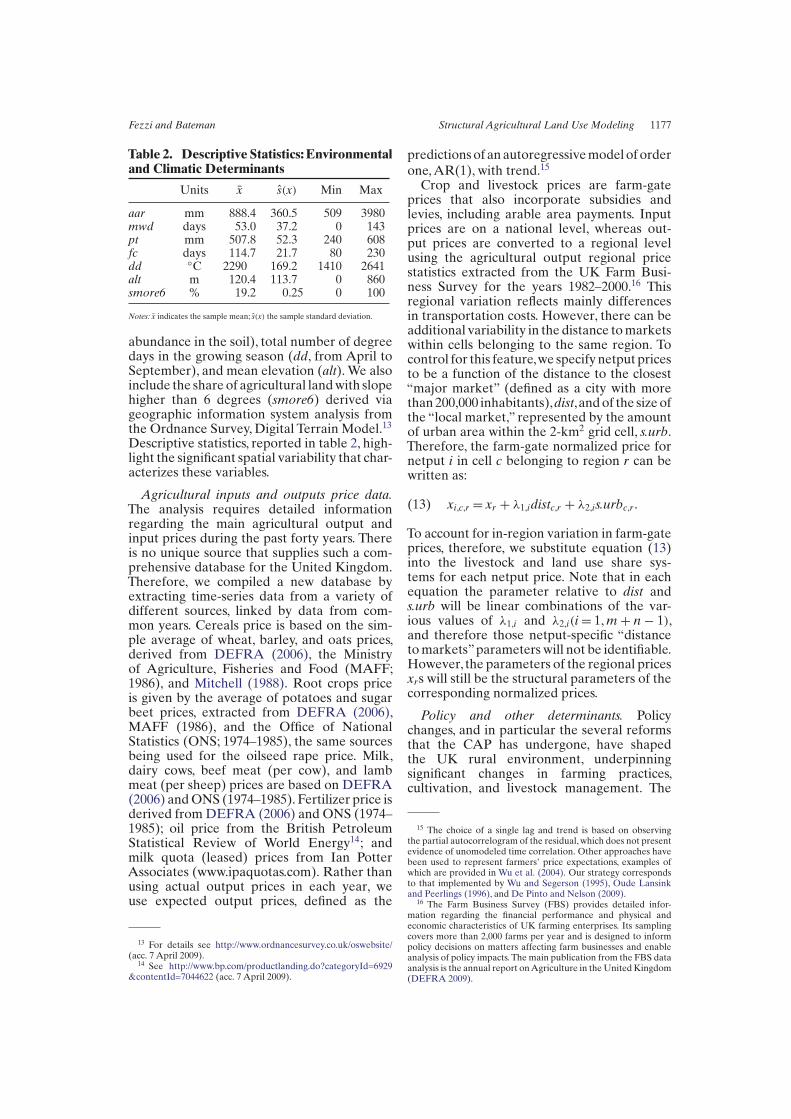
Table 2. Descriptive Statistics: Environmentaland Climatic Determinants
Units x s(x) Min Max
aar mm 888.4 360.5 509 3980mwd days 53.0 37.2 0 143pt mm 507.8 52.3 240 608fc days 114.7 21.7 80 230dd ◦C 2290 169.2 1410 2641alt m 120.4 113.7 0 860smore6 % 19.2 0.25 0 100
Notes: x indicates the sample mean; s(x) the sample standard deviation.
abundance in the soil), total number of degreedays in the growing season (dd, from April toSeptember), and mean elevation (alt).We alsoinclude the shareof agricultural landwith slopehigher than 6 degrees (smore6) derived viageographic information system analysis fromthe Ordnance Survey,Digital Terrain Model.13
Descriptive statistics, reported in table 2, high-light the significant spatial variability that char-acterizes these variables.
Agricultural inputs and outputs price data.The analysis requires detailed informationregarding the main agricultural output andinput prices during the past forty years. Thereis no unique source that supplies such a com-prehensive database for the United Kingdom.Therefore, we compiled a new database byextracting time-series data from a variety ofdifferent sources, linked by data from com-mon years. Cereals price is based on the sim-ple average of wheat, barley, and oats prices,derived from DEFRA (2006), the Ministryof Agriculture, Fisheries and Food (MAFF;1986), and Mitchell (1988). Root crops priceis given by the average of potatoes and sugarbeet prices, extracted from DEFRA (2006),MAFF (1986), and the Office of NationalStatistics (ONS; 1974–1985), the same sourcesbeing used for the oilseed rape price. Milk,dairy cows, beef meat (per cow), and lambmeat (per sheep) prices are based on DEFRA(2006) andONS (1974–1985). Fertilizer price isderived fromDEFRA (2006) and ONS (1974–1985); oil price from the British PetroleumStatistical Review of World Energy14; andmilk quota (leased) prices from Ian PotterAssociates (www.ipaquotas.com). Rather thanusing actual output prices in each year, weuse expected output prices, defined as the
13 For details see http://www.ordnancesurvey.co.uk/oswebsite/(acc. 7 April 2009).14 See http://www.bp.com/productlanding.do?categoryId=6929
&contentId=7044622 (acc. 7 April 2009).
predictionsof anautoregressivemodeloforderone,AR(1), with trend.15
Crop and livestock prices are farm-gateprices that also incorporate subsidies andlevies, including arable area payments. Inputprices are on a national level, whereas out-put prices are converted to a regional levelusing the agricultural output regional pricestatistics extracted from the UK Farm Busi-ness Survey for the years 1982–2000.16 Thisregional variation reflects mainly differencesin transportation costs. However, there can beadditional variability in the distance tomarketswithin cells belonging to the same region. Tocontrol for this feature,we specify netput pricesto be a function of the distance to the closest“major market” (defined as a city with morethan200,000 inhabitants),dist,andof the size ofthe “local market,” represented by the amountof urban area within the 2-km2 grid cell, s.urb.Therefore, the farm-gate normalized price fornetput i in cell c belonging to region r can bewritten as:
(13) xi,c,r = xr + λ1,idistc,r + λ2,is.urbc,r .
To account for in-region variation in farm-gateprices, therefore, we substitute equation (13)into the livestock and land use share sys-tems for each netput price. Note that in eachequation the parameter relative to dist ands.urb will be linear combinations of the var-ious values of λ1,i and λ2,i(i = 1,m + n − 1),and therefore those netput-specific “distancetomarkets”parameters will not be identifiable.However, the parameters of the regional pricesxrs will still be the structural parameters of thecorresponding normalized prices.
Policy and other determinants. Policychanges, and in particular the several reformsthat the CAP has undergone, have shapedthe UK rural environment, underpinningsignificant changes in farming practices,cultivation, and livestock management. The
15 The choice of a single lag and trend is based on observingthe partial autocorrelogram of the residual,which does not presentevidence of unomodeled time correlation. Other approaches havebeen used to represent farmers’ price expectations, examples ofwhich are provided in Wu et al. (2004). Our strategy correspondsto that implemented by Wu and Segerson (1995), Oude Lansinkand Peerlings (1996), and De Pinto and Nelson (2009).16 The Farm Business Survey (FBS) provides detailed infor-
mation regarding the financial performance and physical andeconomic characteristics of UK farming enterprises. Its samplingcovers more than 2,000 farms per year and is designed to informpolicy decisions on matters affecting farm businesses and enableanalysis of policy impacts. The main publication from the FBS dataanalysis is the annual report onAgriculture in theUnitedKingdom(DEFRA 2009).
1178 July 2011 Amer. J. Agr. Econ.
subsidies directly linked to specific crop orlivestock productions, such as the interventionprices, are already included in the output andinput prices. In addition, we include bothspace-variable and space-invariant policydrivers. In the latter group we include the rateof compulsory set-aside and the milk (leased)quota price. In the former group we incorpo-rate those area-specific policy measures thatvary by both time and space. Specifically, wecalculate the share of each grid square in eachyear which is designated as National Park,Nitrate Vulnerable Zone (NVZ) or Envi-ronmentally Sensitive Area (ESA).17 NVZs,established in 1996 and extended in 2003 and2008, have been designed to reduce surfaceand groundwater nitrate contamination incompliance with the EU Nitrate Directive(European Council 1991). The range of mea-sures enforced in NVZs does not go beyondgood agricultural practice, and thereforewhile being mandatory and uncompensated,these are not expected to significantly changeagricultural land use shares. ESAs, introducedin 1987 and subject to various extensions insubsequent years, were launched to safeguardand enhance areas of particularly high land-scape, wildlife, or historic value. Participationin ESA schemes is voluntary, and farmersreceive monetary compensation for engagingin environmentally friendly farming practices,such as converting arable land to permanentgrassland, establishing hedgerows, etc.
Estimation Results and ForecastingPerformance
We implement the QML approach fromequation (12) to estimate two censored, het-eroskedastic Tobit systems: the three-livestock(dairy cattle, beef cattle, sheep) intensity sys-tem from equation (7) and the six land use(cereal, oilseed rape, root crops, temporarygrassland, permanent grassland, rough graz-ing) shares system from equation (9). Selectingas starting values the parameter estimates ofunivariate, heteroskedastic Tobit models andusing the Newton–Raphson method as themaximization algorithm, the QML approachconverges in a convenient length of time forboth systems.18 We discard from the model
17 Digital boundaries at a field level for National Parks, NVZsand ESAs in each year have been downloaded from MAGIC(www.magic.gov.uk).18 We estimate the model using the ml function in Stata 10.1
runningona1.86GHz IntelCore 2Duoprocessor,with 2GBRAM.The six-equation land use shares system converges in just over six
the normalized price parameters that presenta high collinearity (but always retain the ownprice and fertilizer price) to improve the esti-mates of the remaining ones, since the agricul-tural price variables in our sample, as in moststudies, are characterized by a high degree ofcorrelation.19
We do not estimate the model on the entiresample of about 580,000 observations becauseof computational reasons and concerns aboutpossible spatial autocorrelation in the resid-uals. In our framework, among the possiblecauses of residual spatial correlation are unob-servable spatially correlated variables, spa-tial spillovers, and measurement errors due,for example, to spatial aggregation (Anselin1988). Ignoring such issues within a censoredregression may lead to biased and inconsis-tent parameter estimates. In order to decreasethe computational burden and remove resid-ual spatial autocorrelation, we estimate themodel using only a fraction of the origi-nal data selected via spatial sampling (e.g.,Carrión-Flores and Irwin 2004; Nelson andHellerstein 1997). This is defined by randomlyextracting one grid square and then samplingevery fourth grid cell along both latitude andlongitude axes (i.e., considering only the cor-ner grids in a four by four square of cells),leaving a subsample of roughly 30,000 obser-vations (about 5% of the original data). Fol-lowing Carrión-Flores and Irwin (2004), weassess the robustness of our results by compar-ing the parameters’ estimates obtained fromthis samplewith those derived fromalternativesampling methods: two different spatial sam-pling schemes (sampling the fifth and eighthgrid square in both dimensions) and a ran-dom selection of 5% of the data in eachyear.20 Since cell-specific omitted factors canbe present in our data,we allow the residuals tobe correlated among observations pertaining
hours, whereas the three-equation livestock system requires onlyten minutes.19 Despite the high-correlations, the price coefficients appear to
be fairly stable across specifications: there is no change in signif-icance or sign of any of the retained price parameters when theprices of the other outputs are included in the equations (the onlyexception is the parameter on fertilizer price in the permanentgrassland equation, which changes from insignificant to slightlysignificant, but remains very low in magnitude).20 Recalling the discussion of the previous subsection, in all the
sampling schemes we classify as outliers (and exclude from theestimation samples) those grid cells in which the JAC rescalingprocess would be too substantial. We define such cases as those inwhich: (a) the difference between the sum of the agricultural landuse areas from the JAC and the total agricultural area accordingto the ALC is higher than the total grid cell size of 400 ha or (b)
the ratio of these two agricultural areas is greater than 4 or smallerthan 1/4. This roughly corresponds to 7% of the observations.
Fezzi and Bateman Structural Agricultural Land Use Modeling 1179
Table 3. Z-Tests of Parameter Invariance
Land Use Share System Livestock Intensity System(363 parameters) (198 parameters)
Sample N % Reject Max Mean % Reject Max Mean
A 19085 3.5 2.56 0.72 1.5 2.66 0.73B 7539 1.7 2.73 0.61 2.0 2.18 0.67C 29890 11.0 6.38 0.91 1.0 2.19 0.63
Notes:The z-tests assess the null hypothesis that all the parameters are not significantly different from those estimated using the base sampling scheme: randomly
sample one cell and then keep one cell every four in both latitude and longitude axes (total number of observations= 29,860). SampleA= like the base scheme,
but keeping one cell every five; sample B= like the base scheme, but keeping one cell in every eight. In those sampling schemes, the sampled cells are the same
in every year. Sample C = randomly sample 5% of the cells in each year. Since the samples are drawn independently, indicating with βX the parameter and
with VβX the covariance matrix in sample X, the test is: z= (βA − βX)/[VβA +VβX]1/2 , which is asymptotically distributed as a standard normal. These are
the same tests reported in Carrión-Flores and Irwin (2004). “% reject” indicates the percentage of times the test is rejected at the 95% level, “max” indicates
the maximum value of the z-test, and “mean” the average value (both in absolute values).
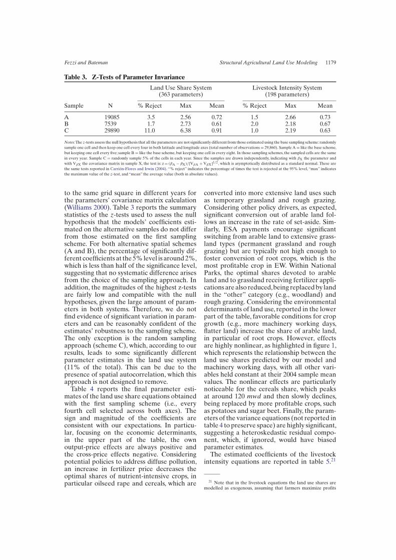
to the same grid square in different years forthe parameters’ covariance matrix calculation(Williams 2000). Table 3 reports the summarystatistics of the z-tests used to assess the nullhypothesis that the models’ coefficients esti-mated on the alternative samples do not differfrom those estimated on the first samplingscheme. For both alternative spatial schemes(A and B), the percentage of significantly dif-ferent coefficients at the5%level is around2%,which is less than half of the significance level,suggesting that no systematic difference arisesfrom the choice of the sampling approach. Inaddition, the magnitudes of the highest z-testsare fairly low and compatible with the nullhypotheses, given the large amount of param-eters in both systems. Therefore, we do notfind evidence of significant variation in param-eters and can be reasonably confident of theestimates’ robustness to the sampling scheme.The only exception is the random samplingapproach (scheme C), which, according to ourresults, leads to some significantly differentparameter estimates in the land use system(11% of the total). This can be due to thepresence of spatial autocorrelation, which thisapproach is not designed to remove.Table 4 reports the final parameter esti-
mates of the land use share equations obtainedwith the first sampling scheme (i.e., everyfourth cell selected across both axes). Thesign and magnitude of the coefficients areconsistent with our expectations. In particu-lar, focusing on the economic determinants,in the upper part of the table, the ownoutput-price effects are always positive andthe cross-price effects negative. Consideringpotential policies to address diffuse pollution,an increase in fertilizer price decreases theoptimal shares of nutrient-intensive crops, inparticular oilseed rape and cereals, which are
converted into more extensive land uses suchas temporary grassland and rough grazing.Considering other policy drivers, as expected,significant conversion out of arable land fol-lows an increase in the rate of set-aside. Sim-ilarly, ESA payments encourage significantswitching from arable land to extensive grass-land types (permanent grassland and roughgrazing) but are typically not high enough tofoster conversion of root crops, which is themost profitable crop in EW. Within NationalParks, the optimal shares devoted to arableland and to grassland receiving fertilizer appli-cations arealso reduced,being replacedby landin the “other” category (e.g., woodland) andrough grazing. Considering the environmentaldeterminants of land use, reported in the lowerpart of the table, favorable conditions for cropgrowth (e.g., more machinery working days,flatter land) increase the share of arable land,in particular of root crops. However, effectsare highly nonlinear, as highlighted in figure 1,which represents the relationship between theland use shares predicted by our model andmachinery working days, with all other vari-ables held constant at their 2004 sample meanvalues. The nonlinear effects are particularlynoticeable for the cereals share, which peaksat around 120 mwd and then slowly declines,being replaced by more profitable crops, suchas potatoes and sugar beet. Finally, the param-eters of the variance equations (not reported intable 4 to preserve space) are highly significant,suggesting a heteroskedastic residual compo-nent, which, if ignored, would have biasedparameter estimates.The estimated coefficients of the livestock
intensity equations are reported in table 5.21
21 Note that in the livestock equations the land use shares aremodelled as exogenous, assuming that farmers maximize profits

1180 July 2011 Amer. J. Agr. Econ.
Table 4. Land Use Share Equations Parameter Estimates
Oilseed Root Temp. Perm. RoughCereals Rape Crops Grassland Grassland Grazing
Pcereals 0.132∗∗∗ – – −0.047∗∗ – –Prape – 0.148∗∗∗∗ – – – –Prootcrops – – 0.037∗ – – –Pfertilizer −0.110∗∗∗ −0.284∗∗∗∗ −0.023∗ 0.069∗∗∗ −0.018 0.035∗∗∗
Set-aside rate −0.425∗∗∗∗ −0.116∗∗∗∗ 0.004 −0.010 −0.033 −0.025∗∗
ESA share −0.033∗∗∗ −0.005 −0.001 0.001 0.039∗∗ 0.030∗∗
Park share −0.020∗ −0.004 −0.003∗ −0.018∗ −0.062∗ 0.042∗
Urban share −0.056∗∗ −0.018∗∗ −0.004 −0.011∗ 0.082∗∗∗ 0.001Distance to major city −0.002 −0.016∗∗∗∗ 0.003 −0.010∗∗ −0.036∗∗∗ 0.008∗
smore6 −0.087∗∗∗ −0.019∗∗∗ −0.004 −0.006 0.128∗∗∗ 0.052∗∗∗∗
alt 13.961∗∗∗ 3.027∗∗ −3.466∗∗∗ −1.072 # #alt2 6.288∗∗ 1.672∗ −1.070∗ −0.745 # #alt <200m # # # # −0.068∗∗∗ 0.007alt >200m # # # # 0.084 −0.154∗
I(alt >200m) # # # # −26.791 21.956mwd 4.170∗∗∗∗ 0.332 1.575∗∗∗∗ 1.107∗∗∗ −7.832∗∗ −0.751mwd2 −1.303 −0.425 0.677∗∗ 0.152 −1.229 0.262pt 6.625∗ 1.011 0.217 −3.582∗ −25.853∗∗ 13.096∗∗
pt2 −2.749 −1.047 0.484 3.845∗ 5.663 −7.614∗∗
fc −4.807 −8.274∗∗ −1.742∗∗ 0.942 6.432 5.164fc2 17.188∗∗ −6.514∗ 2.568∗∗ −6.479∗ −21.100∗ 4.998dd −4.312 0.436 −4.767∗∗∗ 3.562∗∗ 34.183∗∗∗ −6.103∗
dd2 2.540 0.269 1.646∗∗ −1.375 −2.279 −1.370aar −3.193 −9.643∗∗∗ 5.128∗∗∗∗ 5.655∗∗ 0.137 7.930aar2 −1.055 −6.777∗∗ 1.612∗∗ 4.688∗∗ −4.474 6.981∗
Trend 0.0156 0.284∗∗∗∗ −0.018∗∗∗ −0.153∗∗∗∗ −0.103∗∗∗ 0.044∗∗∗
Const 41.276∗∗∗ −13.65∗∗∗ 5.492∗∗∗∗ 16.550∗∗∗ 40.583∗∗ −1.609
Notes:To preserve space the residual correlations, the parameters corresponding to the variance equations and those of the environmental factors interactions
are not reported in the table, but are available under request from the authors. Environmental determinants included as orthogonal polynomials to eliminate
correlation between the linear and the quadratic terms. – = variable removed because of collinearity with the other prices, # = parameter not included in the
equation, * = t-stat >2, ** = t-stat >3, *** = t-stat >4, **** = t-stat >10. All variables defined as in table 1. N= 29,860.
These parameters are structural, in the sensethat they are the same ones appearing in theprofit function. The exceptions are the con-stant terms, which cannot be identified as theαis appearing in equation (6), since they alsocapture the average impacts of all the pos-sible omitted factors. Of course, profits datawould not only allow this identification butalso promote more efficient estimation of theremaining parameters.
in a two-step process and, therefore, treat land use allocations asfixed factors in the netput equations. This is the same approachemployed by Arnade and Kelch (2007) and stems directly fromthe Chambers and Just (1989) profit function maximization. Usingunivariate Tobit models we empirically compare two estimationapproaches: the standard ML which assumes that the land useshares are exogenous and a ML with instrumental variables tomodel land use shares as endogenous. The first strategy providessignificantly superior out-of-sample performance for each of thethree livestock equations. This suggests that, at least in our sam-ple, land use allocation choices are planned on a longer-run basisand can be considered as fixed when evaluating livestock intensitydecisions.
Figure 1. Relationships among predicted landuse shares and machinery working days
Notes: Predicted shares and asymptotic 95% confidence intervals; all other
explanatory variables fixed at their average levels in year 2004.
Fezzi and Bateman Structural Agricultural Land Use Modeling 1181
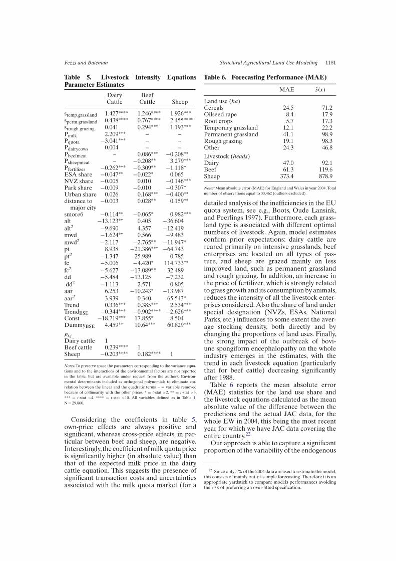
Table 5. Livestock Intensity EquationsParameter Estimates
Dairy BeefCattle Cattle Sheep
stemp.grassland 1.427∗∗∗∗ 1.246∗∗∗∗ 1.926∗∗∗
sperm.grassland 0.438∗∗∗∗ 0.767∗∗∗∗ 2.455∗∗∗∗
srough.grazing 0.041 0.294∗∗∗ 1.193∗∗∗
Pmilk 2.209∗∗∗ – –Pquota −3.041∗∗∗ – –Pdairycows 0.004 – –Pbeefmeat – 0.086∗∗∗ −0.208∗∗
Psheepmeat – −0.208∗∗ 3.279∗∗∗
Pfertilizer −0.262∗∗∗ −0.309∗∗ −1.118∗
ESA share −0.047∗∗ −0.022∗ 0.065NVZ share −0.005 0.010 −0.146∗∗∗
Park share −0.009 −0.010 −0.307∗
Urban share 0.026 0.168∗∗∗ −0.400∗∗
distance to −0.003 0.028∗∗ 0.159∗∗
major citysmore6 −0.114∗∗ −0.065∗ 0.982∗∗∗
alt −13.123∗∗ 0.405 −36.604alt2 −9.690 4.357 −12.419mwd −1.624∗∗ 0.566 −9.483mwd2 −2.117 −2.765∗∗ −11.947∗
pt 8.938 −21.386∗∗∗ −64.743pt2 −1.347 25.989 0.785fc −5.006 −4.420∗ 114.733∗∗
fc2 −5.627 −13.089∗∗ 32.489dd −5.484 −13.125 −7.232dd2 −1.113 2.571 0.805aar 6.253 −10.243∗ −13.987aar2 3.939 0.340 65.543∗
Trend 0.336∗∗∗ 0.385∗∗∗ 2.534∗∗∗
TrendBSE −0.344∗∗∗ −0.902∗∗∗∗ −2.626∗∗∗
Const −18.719∗∗∗ 17.855∗ 8.504DummyBSE 4.459∗∗ 10.64∗∗∗ 60.829∗∗∗
ρi,jDairy cattle 1Beef cattle 0.239∗∗∗∗ 1Sheep −0.203∗∗∗∗ 0.182∗∗∗∗ 1
Notes:To preserve space the parameters corresponding to the variance equa-
tions and to the interactions of the environmental factors are not reported
in the table, but are available under request from the authors. Environ-
mental determinants included as orthogonal polynomials to eliminate cor-
relation between the linear and the quadratic terms. – = variable removed
because of collinearity with the other prices, * = t-stat >2, ** = t-stat >3,
*** = t-stat >4, **** = t-stat >10. All variables defined as in Table 1.
N= 29,860.
Considering the coefficients in table 5,own-price effects are always positive andsignificant, whereas cross-price effects, in par-ticular between beef and sheep, are negative.Interestingly,the coefficient ofmilk quotapriceis significantly higher (in absolute value) thanthat of the expected milk price in the dairycattle equation. This suggests the presence ofsignificant transaction costs and uncertaintiesassociated with the milk quota market (for a
Table 6. Forecasting Performance (MAE)
MAE s(x)
Land use (ha)Cereals 24.5 71.2Oilseed rape 8.4 17.9Root crops 5.7 17.3Temporary grassland 12.1 22.2Permanent grassland 41.1 98.9Rough grazing 19.1 98.3Other 24.3 46.8
Livestock (heads)Dairy 47.0 92.1Beef 61.3 119.6Sheep 373.4 878.9
Notes:Mean absolute error (MAE) for England andWales in year 2004. Total
number of observations equal to 33,462 (outliers excluded).
detailed analysis of the inefficiencies in the EUquota system, see e.g., Boots, Oude Lansink,and Peerlings 1997). Furthermore, each grass-land type is associated with different optimalnumbers of livestock. Again, model estimatesconfirm prior expectations: dairy cattle arereared primarily on intensive grasslands, beefenterprises are located on all types of pas-ture, and sheep are grazed mainly on lessimproved land, such as permanent grasslandand rough grazing. In addition, an increase inthe price of fertilizer, which is strongly relatedto grass growthand its consumptionbyanimals,reduces the intensity of all the livestock enter-prises considered.Also the share of land underspecial designation (NVZs, ESAs, NationalParks, etc.) influences to some extent the aver-age stocking density, both directly and bychanging the proportions of land uses. Finally,the strong impact of the outbreak of bovi-une spongiform encephalopathy on the wholeindustry emerges in the estimates, with thetrend in each livestock equation (particularlythat for beef cattle) decreasing significantlyafter 1988.Table 6 reports the mean absolute error
(MAE) statistics for the land use share andthe livestock equations calculated as the meanabsolute value of the difference between thepredictions and the actual JAC data, for thewhole EW in 2004, this being the most recentyear for which we have JAC data covering theentire country.22
Our approach is able to capture a significantproportion of the variability of the endogenous
22 Since only 5%of the 2004 data are used to estimate themodel,this consists of mainly out-of-sample forecasting. Therefore it is anappropriate yardstick to compare models performances avoidingthe risk of preferring an over-fitted specification.
1182 July 2011 Amer. J. Agr. Econ.
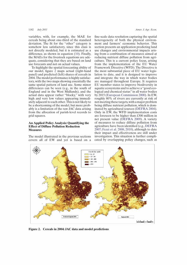
variables, with, for example, the MAE forcereals being about one-third of the standarddeviation. The fit for the “other” category issomehow less satisfactory, since this class isnot directly modeled, but it is estimated as adifference, as shown in equation (10). Finally,the MAEs for the livestock equations are ade-quate, considering that they are based on landuse forecasts and not on actual values.To highlight the spatial forecasting ability of
our model, figure 2 maps actual (right-handpanel) and predicted (left) shares of cereals in2004.Themodel performance is highly satisfac-tory,with the twomaps showing essentially thesame spatial pattern of land use. Some minordifferences can be seen (e.g., in the south ofEngland and in the West Midlands), and theactual data appear rather “blocky,” with veryhigh and very low values appearing immedi-ately adjacent to each other.This is not likely tobe a shortcoming of the model, but more prob-ably is a limitation of the raw JAC data arisingfrom the allocation of parish-level records togrid squares.
An Applied Policy Analysis: Quantifying theEffect of Diffuse Pollution ReductionMeasures
The model illustrated in the previous sectionscovers all of EW and yet is based on a
fine-scale data resolution capturing the spatialheterogeneity of both the physical environ-ment and farmers’ economic behavior. Thissection presents an application predicting landuse changes and environmental impacts aris-ing from a combination of measures aimed atreducing nutrient diffuse pollution from agri-culture. This is a current policy focus, arisingfrom the implementation of the EU WaterFramework Directive (WFD).The Directive isthe most substantial piece of EU water legis-lation to date, and it is designed to improveand integrate the way in which water bodiesare managed throughout Europe. It requiresEU member states to improve biodiversity inaquatic ecosystems and to achieve a“good eco-logical and chemical status” in all water bodiesby 2015 (European Commission 2000). In EW,roughly 80% of rivers are currently at risk ofnotmeeting these targets,withamajorproblembeing diffuse nutrient pollution, which is dom-inated by agricultural sources (DEFRA 2004).Only in EW, the WFD implementation costsare foreseen to be higher than £300 million innet present value (DEFRA 2009). A varietyof measures to reduce diffuse pollution fromagriculture have been identified (e.g.,DEFRA2007; Fezzi et al. 2008, 2010), although to datetheir impact and effectiveness are still underinvestigation. This situation is further compli-cated by overlapping policy changes, such as
Figure 2. Cereals in 2004: JAC data and model predictions

Fezzi and Bateman Structural Agricultural Land Use Modeling 1183
the ongoing reform of the CAP, and externalpressures, such as long-term shifts in fooddemand and climate change. Our approachincludes, in a common framework,market,pol-icy, and environmental drivers and thereforecan be used to test complex scenarios, involv-ing simultaneous changes of multiple factors.However, in order to isolate the effect of possi-ble WFD implementation measures, we focusin this simulation solely upon nutrient reduc-tion measures, holding all the other driversstable at their baseline levels (year 2004).To address the requirements of the WFD, a
joint initiative by DEFRA, the Environmen-tal Agency, and English Nature has identifiedforty catchments across England as priorityareas for action and, via the Catchment Sensi-tive Farming Programme (CSFP), is providingboth advice anddirect payments aimedat influ-encing farming practices so as to reduce diffusewater pollution. In our simulation,we estimatethe changes in land use and livestock numbersin these priority catchments arising from twopossible nutrient leaching reduction measures:(a) a tax on fertilizer of £50/tonne, (b) designa-tion of these areas as ESAs. We also addressthe implication of these two measures for dif-fuse pollution by calculating the correspondingchanges in nitrogen (N) soil balance using theapproach developed by Lord, Anthony, andGoodlass (2002).Nutrient balance calculation is very trans-
parent and relatively insensitive to variation inweather conditions, and it has been proposed
as an indicator of agricultural diffuse pollutionby various international organizations (e.g., theOrganisation for Economic Co-operation andDevelopment; OECD 2001). The approach isstraightforward and consists of calculating thedifference between the N inputs received bythe soil (e.g., fertilizer,manure) and the conse-quent outputs (e.g., harvested matter removedfrom the field, including grass grazed by thelivestock). Each agricultural activity, therefore,produces a nutrient surplus that is retained inthe soil and will eventually leach to the wateraccording to site-specific factors such as soiltexture, slope, and rainfall. The N surplus indi-cates the nitrogen available for leaching fromagriculture given a certain land use. In a rel-atively small country such as the UK, there islittle variation in fertilizer inputs for a givencrop, and therefore a single national set ofsurplus values for crops is appropriate (Lord,Anthony, and Goodlass 2002). Consideringgrassland,on the other hand,N application canchange greatly, from roughly zero tomore than400 kg/ha, according to the livestock intensity.Therefore, adopting an N surplus per head oflivestock approach is a more accurate rep-resentation of nutrient balance for this landuse (Jarvis 2000; Lord,Anthony, and Goodlass2002).Results from our two scenarios are detailed
in table 7. The first column reports estimatesof the N surplus per hectare (or livestockhead) per year arising from each agriculturalactivity (derived from tables 1 and 4 of Lord,
Table 7. Policy Simulation Results and Year 2004 Baseline (model and JAC data)
JAC Rescaled Data Model Predictions (changes in land use)
£50 Fertilizer ESAAnnual N Surplus Baseline Baseline Tax Increase
(Kg N ha−1) (10,000 ha) (10,000 ha) (%) (%)Cereals 47.5 125.0 125.5 −0.9 −10.5Oilseed rape 101.9 18.3 15.6 −15.0 −10.6Root crops 65.8 16.1 10.3 −1.4 −2.9Temp. grass 0 36.5 33.1 2.2 −1.5Perm. grass 0 155.1 162.0 −0.1 10.0Rough grazing 0 50.0 43.0 0.9 28.5Other 25.6 82.2 93.6 2.9 −11.5
(Kg N head−1) (10,000 heads) (10,000 ha) (%) (%)Dairy 63.7 103.1 79.5 −1.9% −11.5%Beef 43.1 186.3 171.9 −1.5% 4.2%Sheep 5.9 783.6 800.3 −1.4% 10.3%
Notes:Results refer only to grid squares included in priority Catchments Sensitive Farming areas. Nitrate surplus per year taken from Tables 1 and 4 in Lord,
Anthony and Goodlass (2002). N surplus for “root crops” given by the average of sugar beet and potatoes, for “other” calculated by using the proportions of
woodland, set aside, horticulture and other arable crops in year 2004 JAC. For dairy and beef cattle calculated by using the proportions of adult, followers and
young cattle in year 2004 JAC. For sheep calculated by using the proportion of sheep and lambs in year 2004 JAC.
1184 July 2011 Amer. J. Agr. Econ.
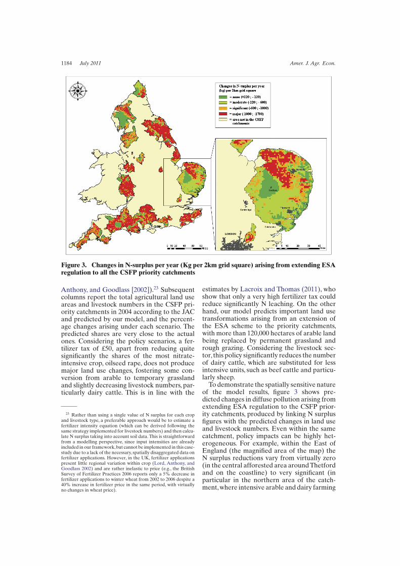
Figure 3. Changes in N-surplus per year (Kg per 2km grid square) arising from extending ESAregulation to all the CSFP priority catchments
Anthony, and Goodlass [2002]).23 Subsequentcolumns report the total agricultural land useareas and livestock numbers in the CSFP pri-ority catchments in 2004 according to the JACand predicted by our model, and the percent-age changes arising under each scenario. Thepredicted shares are very close to the actualones. Considering the policy scenarios, a fer-tilizer tax of £50, apart from reducing quitesignificantly the shares of the most nitrate-intensive crop, oilseed rape, does not producemajor land use changes, fostering some con-version from arable to temporary grasslandand slightly decreasing livestock numbers, par-ticularly dairy cattle. This is in line with the
23 Rather than using a single value of N surplus for each cropand livestock type, a preferable approach would be to estimate afertilizer intensity equation (which can be derived following thesame strategy implemented for livestock numbers) and then calcu-late N surplus taking into account soil data. This is straightforwardfrom a modelling perspective, since input intensities are alreadyincluded in our framework,but cannot be implemented in this case-study due to a lack of the necessary, spatially disaggregated data onfertilizer applications. However, in the UK, fertilizer applicationspresent little regional variation within crop (Lord, Anthony, andGoodlass 2002) and are rather inelastic to price (e.g., the BritishSurvey of Fertilizer Practices 2006 reports only a 5% decrease infertilizer applications to winter wheat from 2002 to 2006 despite a40% increase in fertilizer price in the same period, with virtuallyno changes in wheat price).
estimates by Lacroix and Thomas (2011), whoshow that only a very high fertilizer tax couldreduce significantly N leaching. On the otherhand, our model predicts important land usetransformations arising from an extension ofthe ESA scheme to the priority catchments,with more than 120,000 hectares of arable landbeing replaced by permanent grassland andrough grazing. Considering the livestock sec-tor, this policy significantly reduces the numberof dairy cattle, which are substituted for lessintensive units, such as beef cattle and particu-larly sheep.To demonstrate the spatially sensitive nature
of the model results, figure 3 shows pre-dicted changes in diffuse pollution arising fromextending ESA regulation to the CSFP prior-ity catchments, produced by linking N surplusfigures with the predicted changes in land useand livestock numbers. Even within the samecatchment, policy impacts can be highly het-erogeneous. For example, within the East ofEngland (the magnified area of the map) theN surplus reductions vary from virtually zero(in the central afforested area aroundThetfordand on the coastline) to very significant (inparticular in the northern area of the catch-ment,where intensive arable and dairy farming

Fezzi and Bateman Structural Agricultural Land Use Modeling 1185
are switched to more extensive agriculturalland uses). On the national scale, variation iseven more noteworthy, with major N surplusreductions typically taking place in the mostagriculturally intensive areas.
Concluding Remarks
This article develops a structural approachencompassing agricultural land use deci-sions, livestock numbers, crop yields, inputapplications, and profits in a coherent and uni-fying framework. The underpinning theoreti-cal model builds upon the joint multi-outputprofit function introduced by Chambers andJust (1989) and is translated into an empiri-cally tractable system of equations by directlyspecifying the profit function as one of theflexible functional forms available in the lit-erature. The system can be estimated onfarm-level or spatially disaggregated data byimplementing a strategy that is robust tothe presence of censored observations. Herewe propose an extension of the QML esti-mator developed by Yen, Lin, and Small-wood (2003) for systems of censored demandequations.A large, spatially explicit, high-resolution
database is compiled and used to empiricallytest this framework. The model is employedwithin a decision-relevant context to exam-ine the impact of policy change using eitherinput taxation or area-based schemes to reducethe incidence of diffuse agricultural pollu-tion of water quality. Policy impacts arefound to be highly spatially heterogeneous,and significantly affect margins that are bothextensive (land use type) and intensive (live-stock numbers). Given the key role that live-stock play in nutrient leaching, this quan-tification is essential to assess environmentalimplications.The findings of this research could be
extended in several directions. First, while inthe methodological section we propose a tech-nique to estimate the entire profit functionsystem, in the empirical application we didnot recover all the structural parameters ofthe model and, therefore, did not derive thewelfare implications of land use change. Farm-level data on profits and yields could be usedto address this limitation and jointly estimatethe entire system of equations (6), (7), and(9). The obvious drawback of this approachwould be loss of the spatial dimension of
the analysis, which could be at least partiallymaintained by knowing the locations of thefarms and linking them to the environmentalcharacteristics. Secondly, this model is gen-eral enough to be implemented in a varietyof empirical contexts. Given the refined spec-ification of the climatic variables, an obviouscandidate is the prediction of the effects ofglobal warming on agriculture. Finally, thisframework is essentially static: an importantextension would be to formulate a dynamiceconometric specification to investigate theintertemporal aspects of agricultural produc-tion decisions.
References
Amemiya, T. 1973. Regression Analysis Whenthe DependentVariable Is Truncated Nor-mal. Econometrica 41: 997–1016.
Anselin, L. 1988. Spatial Econometrics. In ACompanion to Theoretical Econometrics,ed. B. Baltagi, pp. 310–330. Oxford: Black-well.
Antle, J., and S. Capalbo. 2001. Econometric-process models for integrated assessmentof agricultural production systems.Ameri-can Journal of Agricultural Economics 83:389–401.
Antle, J., S. Capalbo, S. Mooney S., E. Elliott,and K. Paustian K. 2003. Spatial hetero-geneity, contract design, and the efficiencyof carbon sequestration policies for agri-culture. Journal of Environmental Eco-nomics and Management, 46: 231–250.
Arnade, C., and D. Kelch. 2007. Estimationof area elasticities from a standard profitfunction.American Journal of AgriculturalEconomics 89: 727–737.
Ball, E. V., J.-C. Bureau, K. Eakin, and A.Somwaru. 1997. Cap reform: modelingsupply response subject to the land set-aside.Agricultural Economics,17:277–288.
Barten, A. P. 1969. Maximum likelihood esti-mation of a complete system of demandequations. European Economic Review 1:7–73.
Boots, M., A. Oude Lansink, and J. Peerlings.1997. Efficiency loss due to distortion inDutch milk quota trade.European Reviewof Agricultural Economics 24: 31–46.
Brady, M., and E. Irwin. 2011. Accounting forspatial effects in economics models of landuse: recent developments and challengesahead. Environmental and Resource Eco-nomics 48: 487–509.
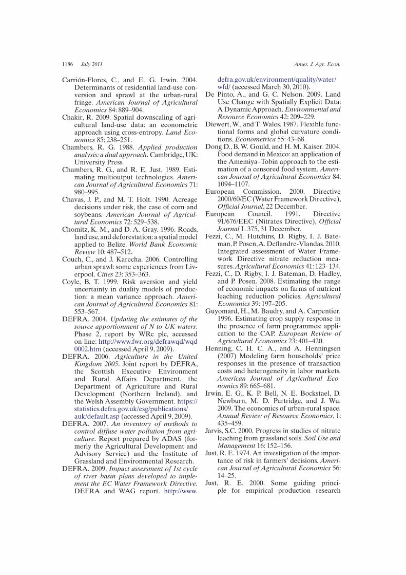
1186 July 2011 Amer. J. Agr. Econ.
Carrión-Flores, C., and E. G. Irwin. 2004.Determinants of residential land-use con-version and sprawl at the urban-ruralfringe. American Journal of AgriculturalEconomics 84: 889–904.
Chakir, R. 2009. Spatial downscaling of agri-cultural land-use data: an econometricapproach using cross-entropy. Land Eco-nomics 85: 238–251.
Chambers, R. G. 1988. Applied productionanalysis: a dual approach. Cambridge,UK:University Press.
Chambers, R. G., and R. E. Just. 1989. Esti-mating multioutput technologies. Ameri-can Journal of Agricultural Economics 71:980–995.
Chavas, J. P., and M. T. Holt. 1990. Acreagedecisions under risk, the case of corn andsoybeans. American Journal of Agricul-tural Economics 72: 529–538.
Chomitz, K. M., and D. A. Gray. 1996. Roads,land use,and deforestation:a spatialmodelapplied to Belize. World Bank EconomicReview 10: 487–512.
Couch, C., and J. Karecha. 2006. Controllingurban sprawl: some experiences from Liv-erpool. Cities 23: 353–363.
Coyle, B. T. 1999. Risk aversion and yielduncertainty in duality models of produc-tion: a mean variance approach. Ameri-can Journal of Agricultural Economics 81:553–567.
DEFRA. 2004. Updating the estimates of thesource apportionment of N to UK waters.Phase 2, report by WRc plc, accessedon line: http://www.fwr.org/defrawqd/wqd0002.htm (accessedApril 9, 2009).
DEFRA. 2006. Agriculture in the UnitedKingdom 2005. Joint report by DEFRA,the Scottish Executive Environmentand Rural Affairs Department, theDepartment of Agriculture and RuralDevelopment (Northern Ireland), andthe Welsh Assembly Government. https://statistics.defra.gov.uk/esg/publications/auk/default.asp (accessedApril 9, 2009).
DEFRA. 2007. An inventory of methods tocontrol diffuse water pollution from agri-culture. Report prepared by ADAS (for-merly the Agricultural Development andAdvisory Service) and the Institute ofGrassland and Environmental Research.
DEFRA. 2009. Impact assessment of 1st cycleof river basin plans developed to imple-ment the EC Water Framework Directive.DEFRA and WAG report. http://www.
defra.gov.uk/environment/quality/water/wfd/ (accessed March 30, 2010).
De Pinto, A., and G. C. Nelson. 2009. LandUse Change with Spatially Explicit Data:ADynamicApproach.Environmental andResource Economics 42: 209–229.
Diewert,W., and T.Wales. 1987. Flexible func-tional forms and global curvature condi-tions. Econometrica 55: 43–68.
Dong D., B.W. Gould, and H. M. Kaiser. 2004.Food demand in Mexico: an application ofthe Amemiya–Tobin approach to the esti-mation of a censored food system.Ameri-can Journal of Agricultural Economics 84:1094–1107.
European Commission. 2000. Directive2000/60/EC(WaterFrameworkDirective),Official Journal, 22 December.
European Council. 1991. Directive91/676/EEC (Nitrates Directive), OfficialJournal L 375, 31 December.
Fezzi, C., M. Hutchins, D. Rigby, I. J. Bate-man,P. Posen,A.Deflandre-Vlandas. 2010.Integrated assessment of Water Frame-work Directive nitrate reduction mea-sures.Agricultural Economics 41: 123–134.
Fezzi, C., D. Rigby, I. J. Bateman, D. Hadley,and P. Posen. 2008. Estimating the rangeof economic impacts on farms of nutrientleaching reduction policies. AgriculturalEconomics 39: 197–205.
Guyomard, H., M. Baudry, and A. Carpentier.1996. Estimating crop supply response inthe presence of farm programmes: appli-cation to the CAP. European Review ofAgricultural Economics 23: 401–420.
Henning, C. H. C. A., and A. Henningsen(2007) Modeling farm households’ priceresponses in the presence of transactioncosts and heterogeneity in labor markets.American Journal of Agricultural Eco-nomics 89: 665–681.
Irwin, E. G., K. P. Bell, N. E. Bockstael, D.Newburn, M. D. Partridge, and J. Wu.2009. The economics of urban-rural space.Annual Review of Resource Economics, 1:435–459.
Jarvis, S.C. 2000. Progress in studies of nitrateleaching from grassland soils. Soil Use andManagement 16: 152–156.
Just,R. E. 1974.An investigation of the impor-tance of risk in farmers’ decisions.Ameri-can Journal of Agricultural Economics 56:14–25.
Just, R. E. 2000. Some guiding princi-ple for empirical production research
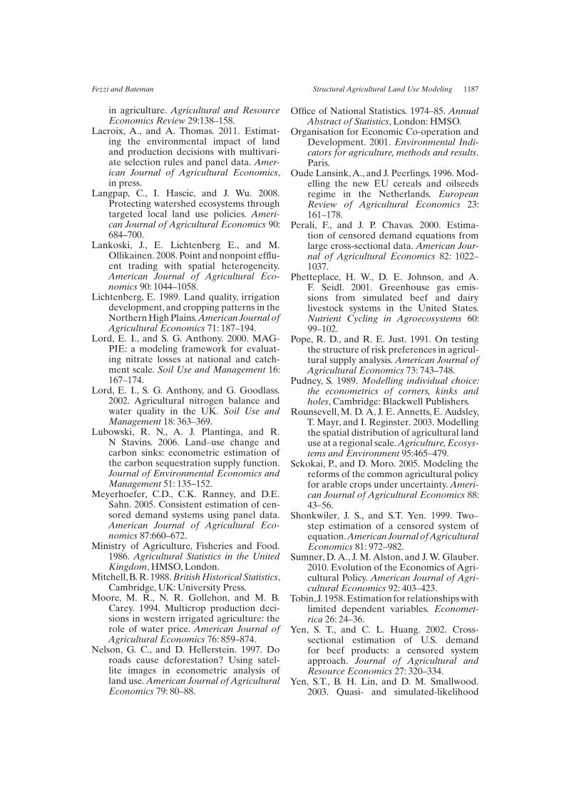
Fezzi and Bateman Structural Agricultural Land Use Modeling 1187
in agriculture. Agricultural and ResourceEconomics Review 29:138–158.
Lacroix, A., and A. Thomas. 2011. Estimat-ing the environmental impact of landand production decisions with multivari-ate selection rules and panel data. Amer-ican Journal of Agricultural Economics,in press.
Langpap, C., I. Hascic, and J. Wu. 2008.Protecting watershed ecosystems throughtargeted local land use policies. Ameri-can Journal of Agricultural Economics 90:684–700.
Lankoski, J., E. Lichtenberg E., and M.Ollikainen. 2008. Point and nonpoint efflu-ent trading with spatial heterogeneity.American Journal of Agricultural Eco-nomics 90: 1044–1058.
Lichtenberg, E. 1989. Land quality, irrigationdevelopment, and cropping patterns in theNorthernHighPlains.American Journal ofAgricultural Economics 71: 187–194.
Lord, E. I., and S. G. Anthony. 2000. MAG-PIE: a modeling framework for evaluat-ing nitrate losses at national and catch-ment scale. Soil Use and Management 16:167–174.
Lord, E. I., S. G. Anthony, and G. Goodlass.2002. Agricultural nitrogen balance andwater quality in the UK. Soil Use andManagement 18: 363–369.
Lubowski, R. N., A. J. Plantinga, and R.N Stavins. 2006. Land–use change andcarbon sinks: econometric estimation ofthe carbon sequestration supply function.Journal of Environmental Economics andManagement 51: 135–152.
Meyerhoefer, C.D., C.K. Ranney, and D.E.Sahn. 2005. Consistent estimation of cen-sored demand systems using panel data.American Journal of Agricultural Eco-nomics 87:660–672.
Ministry of Agriculture, Fisheries and Food.1986. Agricultural Statistics in the UnitedKingdom, HMSO, London.
Mitchell,B.R. 1988.British Historical Statistics,Cambridge, UK:University Press.
Moore, M. R., N. R. Gollehon, and M. B.Carey. 1994. Multicrop production deci-sions in western irrigated agriculture: therole of water price. American Journal ofAgricultural Economics 76: 859–874.
Nelson, G. C., and D. Hellerstein. 1997. Doroads cause deforestation? Using satel-lite images in econometric analysis ofland use.American Journal of AgriculturalEconomics 79: 80–88.
Office of National Statistics. 1974–85. AnnualAbstract of Statistics, London: HMSO.
Organisation for Economic Co-operation andDevelopment. 2001. Environmental Indi-cators for agriculture, methods and results.Paris.
Oude Lansink,A., and J. Peerlings. 1996. Mod-elling the new EU cereals and oilseedsregime in the Netherlands. EuropeanReview of Agricultural Economics 23:161–178.
Perali, F., and J. P. Chavas. 2000. Estima-tion of censored demand equations fromlarge cross-sectional data.American Jour-nal of Agricultural Economics 82: 1022–1037.
Phetteplace, H. W., D. E. Johnson, and A.F. Seidl. 2001. Greenhouse gas emis-sions from simulated beef and dairylivestock systems in the United States.Nutrient Cycling in Agroecosystems 60:99–102.
Pope, R. D., and R. E. Just. 1991. On testingthe structure of risk preferences in agricul-tural supply analysis.American Journal ofAgricultural Economics 73: 743–748.
Pudney, S. 1989. Modelling individual choice:the econometrics of corners, kinks andholes, Cambridge: Blackwell Publishers.
Rounsevell, M. D.A, J. E. Annetts, E. Audsley,T. Mayr, and I. Reginster. 2003. Modellingthe spatial distribution of agricultural landuse at a regional scale.Agriculture, Ecosys-tems and Environment 95:465–479.
Sckokai, P., and D. Moro. 2005. Modeling thereforms of the common agricultural policyfor arable crops under uncertainty.Ameri-can Journal of Agricultural Economics 88:43–56.
Shonkwiler, J. S., and S.T. Yen. 1999. Two–step estimation of a censored system ofequation.American Journal ofAgriculturalEconomics 81: 972–982.
Sumner,D.A., J. M.Alston, and J.W. Glauber.2010. Evolution of the Economics ofAgri-cultural Policy. American Journal of Agri-cultural Economics 92: 403–423.
Tobin,J. 1958.Estimation for relationshipswithlimited dependent variables. Economet-rica 26: 24–36.
Yen, S. T., and C. L. Huang. 2002. Cross-sectional estimation of U.S. demandfor beef products: a censored systemapproach. Journal of Agricultural andResource Economics 27: 320–334.
Yen, S.T., B. H. Lin, and D. M. Smallwood.2003. Quasi- and simulated-likelihood

1188 July 2011 Amer. J. Agr. Econ.
approaches to censored demand systems:food consumption by food stamp recip-ients in the United States. AmericanJournal of Agricultural Economics 85:458–478.
White, H. 1982. Maximum likelihood estima-tion of misspecified models. Econometrica50: 1–25.
Williams,R.L. 2000.A note on robust varianceestimation for cluster–correlated data.Biometrics 56: 645–646.
Wooldridge, J. M. 1995. Selection correc-tions for panel data under conditional
mean independence assumptions. Journalof Econometrics 68: 115–132.
Wu, J., R. M. Adams, C. L. Kling, andK.Tanaka 2004. Frommicrolevel decisionsto landscape changes: an assessment ofagricultural conservation policies. Ameri-can Journal of Agricultural Economics 81:26–41.
Wu, J., and K. Segerson. 1995. The impactof policies and land characteristics onpotential groundwater pollution in Wis-consin. American Journal of AgriculturalEconomics 77: 1033–1047.