Senior Lecturer, Civil Engineering Department, The University of Texas, ECJ Building 6.204, Austin, TX 6

78712

CAR FOLLOWING MODELS

BY RICHARD W. ROTHERY6

T

xf(t)

x5(t)

xf(t)

�x5(t)

�xf(t)

x5(t)

xf(t)

xi(t)

CHAPTER 4 - Frequently used Symbols

� = Numerical coefficientsa = Generalized sensitivity coefficient

5,m

a (t) = Instantaneous acceleration of a followingf

vehicle at time ta (t) = Instantaneous acceleration of a lead

5

vehicle at time t� = Numerical coefficient C = Single lane capacity (vehicle/hour)- = Rescaled time (in units of response time,

T) following vehicle = Short finite time period u (t) = Velocity profile of the lead vehicle of aF = Amplitude factor� = Numerical coefficient k = Traffic stream concentration in vehicles

per kilometer 7 = Frequency of a monochromatic speedk = Jam concentrationj

k = Concentration at maximum flowm

k = Concentration where vehicle to vehiclef

interactions begin = Instantaneous speed of a lead vehicle atk = Normalized concentration time tn

L = Effective vehicle lengthL = Inverse Laplace transform-1

� = Proportionality factor� = Sensitivity coefficient, i = 1,2,3,...i

ln(x) = Natural logarithm of xq = Flow in vehicles per hourq = Normalized flown

<S> = Average spacing rear bumper to rearbumper = Instantaneous position of the following

S = Initial vehicle spacing vehicle at time ti

S = Final vehicle spacing = Instantaneous position of the ith vehicle atf

S = Vehicle spacing for stopped traffic time to

S(t) = Inter-vehicle spacing z(t) = Position in a moving coordinate system�S = Inter-vehicle spacing change

= Average response timeT = Propagation time for a disturbanceo

t = Time

t = Collision timec

T = Reaction timeU = Speed of a lead vehicle

5

U = Speed of a following vehiclef

U = Final vehicle speedf

U = Free mean speed, speed of traffic near zerof

concentrationU = Initial vehicle speedi

U = Relative speed between a lead andrel

5

platoonV = Speed V = Final vehicle speedf

oscillation= Instantaneous acceleration of a following

vehicle at time t

= Instantaneous speed of a following vehicleat time t

= Instantaneous speed of a lead vehicle attime t

= Instantaneous speed of a following vehicleat time t

= Instantaneous position of a lead vehicle attime t

< x > = Average of a variable x

6 = Frequency factor

S ���V��V2

� 0.5(a1f a1

5)

� � �

(4.2)

(4.3)

4.CAR FOLLOWING MODELS

It has been estimated that mankind currently devotes over 10 roadways. The speed-spacing relations that were obtained frommillion man-years each year to driving the automobile, which on these studies can be represented by the following equation:demand provides a mobility unequaled by any other mode oftransportation. And yet, even with the increased interest intraffic research, we understand relatively little of what isinvolved in the "driving task". Driving, apart from walking,talking, and eating, is the most widely executed skill in the worldtoday and possibly the most challenging. where the numerical values for the coefficients, �, �, and � take

Cumming (1963) categorized the various subtasks that are are given below:involved in the overall driving task and paralleled the driver'srole as an information processor (see Chapter 3). This chapterfocuses on one of these subtasks, the task of one vehiclefollowing another on a single lane of roadway (car following).This particular driving subtask is of interest because it isrelatively simple compared to other driving tasks, has beensuccessfully described by mathematical models, and is animportant facet of driving. Thus, understanding car followingcontributes significantly to an understanding of traffic flow. Carfollowing is a relatively simple task compared to the totality oftasks required for vehicle control. However, it is a task that iscommonly practiced on dual or multiple lane roadways whenpassing becomes difficult or when traffic is restrained to a singlelane. Car following is a task that has been of direct or indirectinterest since the early development of the automobile.

One aspect of interest in car following is the average spacing, S,that one vehicle would follow another at a given speed, V. Theinterest in such speed-spacing relations is related to the fact thatnearly all capacity estimates of a single lane of roadway werebased on the equation:

C = (1000) V/S (4.1) permeated safety organizations can be formed. In general, the

where physical length of vehicles; the human-factor element ofC = Capacity of a single lane

(vehicles/hour) V = Speed (km/hour)S = Average spacing rear bumper to rear

bumper in meters

The first Highway Capacity Manual (1950) lists 23observational studies performed between 1924 and 1941 thatwere directed at identifying an operative speed-spacing relationso that capacity estimates could be established for single lanes of

on various values. Physical interpretations of these coefficients

� = the effective vehicle length, L � = the reaction time, T

� = the reciprocal of twice the maximum averagedeceleration of a following vehicle

In this case, the additional term, � V , can provide sufficient2

spacing so that if a lead vehicle comes to a full stopinstantaneously, the following vehicle has sufficient spacing tocome to a complete stop without collision. A typical valueempirically derived for � would be � 0.023 seconds /ft . A less2

conservative interpretation for the non-linear term would be:

where a and a are the average maximum decelerations of theƒ 5

following and lead vehicles, respectively. These terms attemptto allow for differences in braking performances betweenvehicles whether real or perceived (Harris 1964).

For � = 0, many of the so-called "good driving" rules that have

speed-spacing Equation 4.2 attempts to take into account the

perception, decision making, and execution times; and the netphysics of braking performances of the vehicles themselves. Ithas been shown that embedded in these models are theoreticalestimates of the speed at maximum flow, (�/�) ; maximum0.5

flow, [� + 2(� �) ] ; and the speed at which small changes in0.5 -1

traffic stream speed propagate back through a traffic stream,(�/�) (Rothery 1968). 0.5

The speed-spacing models noted above are applicable to caseswhere each vehicle in the traffic stream maintains the same ornearly the same constant speed and each vehicle is attempting to

�� &$5 )2//2:,1*02'(/6

� � �

maintain the same spacing (i.e., it describes a steady-state traffic 1958 by Herman and his associates at the General Motorsstream). Research Laboratories. These research efforts were microscopic

Through the work of Reuschel (1950) and Pipes (1953), the which one vehicle followed another. With such a description,dynamical elements of a line of vehicles were introduced. In the macroscopic behavior of single lane traffic flow can bethese works, the focus was on the dynamical behavior of a approximated. Hence, car following models form a bridgestream of vehicles as they accelerate or decelerate and each between individual "car following" behavior and thedriver-vehicle pair attempts to follow one another. These efforts macroscopic world of a line of vehicles and their correspondingwere extended further through the efforts of Kometani and flow and stability properties.Sasaki (1958) in Japan and in a series of publications starting in

approaches that focused on describing the detailed manner in

4.1 Model Development

Car following models of single lane traffic assume that there is vehicle characteristics or class ofa correlation between vehicles in a range of inter-vehicle characteristics and from the driver's vastspacing, from zero to about 100 to 125 meters and provides an repertoire of driving experience. Theexplicit form for this coupling. The modeling assumes that each integration of current information anddriver in a following vehicle is an active and predictable control catalogued knowledge allows for theelement in the driver-vehicle-road system. These tasks are development of driving strategies whichtermed psychomotor skills or perceptual-motor skills because become "automatic" and from which evolvethey require a continued motor response to a continuous series "driving skills".of stimuli.

The relatively simple and common driving task of one vehicle commands with dexterity, smoothness, andfollowing another on a straight roadway where there is no coordination, constantly relying on feedbackpassing (neglecting all other subsidiary tasks such as steering, from his own responses which arerouting, etc.) can be categorized in three specific subtasks: superimposed on the dynamics of the system's

� Perception: The driver collects relevant informationmainly through the visual channel. This It is not clear how a driver carries out these functions in detail.information arises primarily from the motion The millions of miles that are driven each year attest to the factof the lead vehicle and the driver's vehicle. that with little or no training, drivers successfully solve aSome of the more obvious information multitude of complex driving tasks. Many of the fundamentalelements, only part of which a driver is questions related to driving tasks lie in the area of 'humansensitive to, are vehicle speeds, accelerations factors' and in the study of how human skill is related toand higher derivatives (e.g., "jerk"), inter- information processes. vehicle spacing, relative speeds, rate ofclosure, and functions of these variables (e.g., The process of comparing the inputs of a human operator to thata "collision time"). operator's outputs using operational analysis was pioneered by

� Decision These attempts to determine mathematical expressions linkingMaking: A driver interprets the information obtained by input and output have met with limited success. One of the

sampling and integrates it over time in order to primary difficulties is that the operator (in our case the driver)provide adequate updating of inputs. has no unique transfer function; the driver is a differentInterpreting the information is carried out 'mechanism' under different conditions. While such an approachwithin the framework of a knowledge of has met with limited success, through the course of studies like

� Control: The skilled driver can execute control

counterparts (lead vehicle and roadway).

the work of Tustin (1947), Ellson (1949), and Taylor (1949).

<U5Uf> <Urel>

1 tP

t� t/2

t t/2Urel(t)dt

tc S(t)Urel

�� &$5 )2//2:,1*02'(/6

� � �

(4.5)

(4.6)

these a number of useful concepts have been developed. For where � is a proportionality factor which equates the stimulusexample, reaction times were looked upon as characteristics of function to the response or control function. The stimulusindividuals rather than functional characteristics of the task itself. function is composed of many factors: speed, relative speed, In addition, by introducing the concept of "information", it has inter-vehicle spacing, accelerations, vehicle performance, driverproved possible to parallel reaction time with the rate of coping thresholds, etc. with information.

The early work by Tustin (1947) indicated maximum rates of the question is, which of these factors are the most significant fromorder of 22-24 bits/second (sec). Knowledge of human an explanatory viewpoint. Can any of them be neglected and stillperformance and the rates of handling information made it retain an approximate description of the situation beingpossible to design the response characteristics of the machine for modeled? maximum compatibility of what really is an operator-machinesystem. What is generally assumed in car following modeling is that a

The very concept of treating an operator as a transfer function avoid collisions.implies, partly, that the operator acts in some continuousmanner. There is some evidence that this is not completely These two elements can be accomplished if the driver maintainscorrect and that an operator acts in a discontinuous way. Thereis a period of time during which the operator having made a"decision" to react is in an irreversible state and that the responsemust follow at an appropriate time, which later is consistent withthe task.

The concept of a human behavior being discontinuous incarrying out tasks was first put forward by Uttley (1944) andhas been strengthened by such studies as Telfor's (1931), whodemonstrated that sequential responses are correlated in such away that the response-time to a second stimulus is affectedsignificantly by the separation of the two stimuli. Inertia, on theother hand, both in the operator and the machine, creates anappearance of smoothness and continuity to the control element.

In car following, inertia also provides direct feedback data to theoperator which is proportional to the acceleration of the vehicle.Inertia also has a smoothing effect on the performancerequirements of the operator since the large masses and limitedoutput of drive-trains eliminate high frequency components ofthe task.

Car following models have not explicitly attempted to take all ofthese factors into account. The approach that is used assumesthat a stimulus-response relationship exists that describes, atleast phenomenologically, the control process of a driver-vehicleunit. The stimulus-response equation expresses the concept thata driver of a vehicle responds to a given stimulus according to arelation:

Response = � Stimulus (4.4)

Do all of these factors come into play part of the time? The

driver attempts to: (a) keep up with the vehicle ahead and (b)

a small average relative speed, U over short time periods, sayrel

t, i.e.,

is kept small. This ensures that ‘collision’ times:

are kept large, and inter-vehicle spacings would not appreciablyincrease during the time period, t. The duration of the t willdepend in part on alertness, ability to estimate quantities such as:spacing, relative speed, and the level of information required forthe driver to assess the situation to a tolerable probability level(e.g., the probability of detecting the relative movement of anobject, in this case a lead vehicle) and can be expressed as afunction of the perception time.

Because of the role relative-speed plays in maintaining relativelylarge collision times and in preventing a lead vehicle from'drifting' away, it is assumed as a first approximation that theargument of the stimulus function is the relative speed.

From the discussion above of driver characteristics, relativespeed should be integrated over time to reflect the recent timehistory of events, i.e., the stimulus function should have the formlike that of Equation 4.5 and be generalized so that the stimulus

< U5Uf > <Urel >P

t� t/2

t t/2)(tt �)Urel(t

�)dt

)(t) (tT)

Past

Weightingfunction

Future

Now

Time

(tT) 0, for tgT

(tT) 1, for t T

P�

o (tT)dt 1

T(t) Pt

0t �)(t �)dt �

T

�� &$5 )2//2:,1*02'(/6

� � �

(4.7)

(4.8)

(4.9)

(4.10)

(4.12)

at a given time, t, depends on the weighted sum of all earliervalues of the relative speed, i.e.,

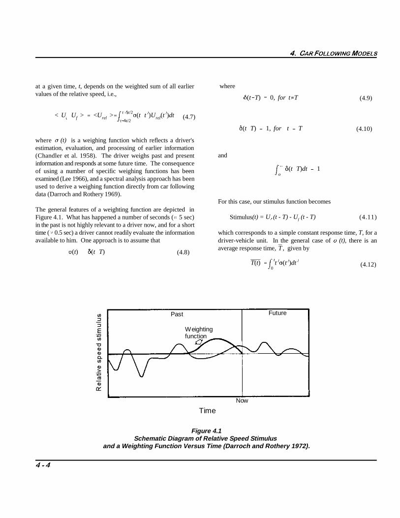
where ) (t) is a weighing function which reflects a driver'sestimation, evaluation, and processing of earlier information(Chandler et al. 1958). The driver weighs past and presentinformation and responds at some future time. The consequenceof using a number of specific weighing functions has beenexamined (Lee 1966), and a spectral analysis approach has beenused to derive a weighing function directly from car followingdata (Darroch and Rothery 1969).

The general features of a weighting function are depicted inFigure 4.1. What has happened a number of seconds (� 5 sec)in the past is not highly relevant to a driver now, and for a shorttime (� 0.5 sec) a driver cannot readily evaluate the information which corresponds to a simple constant response time, T, for aavailable to him. One approach is to assume that

where

and

For this case, our stimulus function becomes

Stimulus(t) = U (t - T) - U (t - T) (4.11)5 f

driver-vehicle unit. In the general case of ) (t), there is anaverage response time, , given by

Figure 4.1Schematic Diagram of Relative Speed Stimulus

and a Weighting Function Versus Time (Darroch and Rothery 1972).

xf(t) �[x.5(tT)x

.f(tT)]

xf(t�T) �[x.5(t)x

.f(t)]

x

�� &$5 )2//2:,1*02'(/6

� � �

(4.14)

(4.15)

The main effect of such a response time or delay is that the driveris responding at all times to a stimulus. The driver is observingthe stimulus and determining a response that will be made sometime in the future. By delaying the response, the driver obtains"advanced" information.

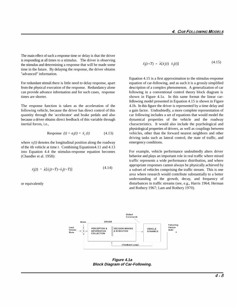
For redundant stimuli there is little need to delay response, apart equation of car-following, and as such it is a grossly simplifiedfrom the physical execution of the response. Redundancy alone description of a complex phenomenon. A generalization of carcan provide advance information and for such cases, response following in a conventional control theory block diagram istimes are shorter. shown in Figure 4.1a. In this same format the linear car-

The response function is taken as the acceleration of the 4.1b. In this figure the driver is represented by a time delay andfollowing vehicle, because the driver has direct control of this a gain factor. Undoubtedly, a more complete representation ofquantity through the 'accelerator' and brake pedals and also car following includes a set of equations that would model thebecause a driver obtains direct feedback of this variable through dynamical properties of the vehicle and the roadwayinertial forces, i.e., characteristics. It would also include the psychological and

Response (t) = a (t) = (t) (4.13) f f

where x (t) denotes the longitudinal position along the roadwayi

of the ith vehicle at time t. Combining Equations4.11 and 4.13into Equation 4.4 the stimulus-response equation becomes(Chandler et al. 1958):

or equivalently

Equation 4.15 is a first approximation to the stimulus-response

following model presented in Equation 4.15 is shown in Figure

physiological properties of drivers, as well as couplings betweenvehicles, other than the forward nearest neighbors and otherdriving tasks such as lateral control, the state of traffic, andemergency conditions.

For example, vehicle performance undoubtedly alters driverbehavior and plays an important role in real traffic where mixedtraffic represents a wide performance distribution, and whereappropriate responses cannot always be physically achieved bya subset of vehicles comprising the traffic stream. This is onearea where research would contribute substantially to a betterunderstanding of the growth, decay, and frequency ofdisturbances in traffic streams (see, e.g., Harris 1964; Hermanand Rothery 1967; Lam and Rothery 1970).

Figure 4.1aBlock Diagram of Car-Following.

xf(-�1) C[(x.5(-)x

.f(-))]

�xn(t) u��vn

)0

(1))t

(n�))T�

n�) -(n�))T n�)1

(n1)!)!& (u0(t-)u)dt

�� &$5 )2//2:,1*02'(/6

� � �

(4.16)

Figure 4.1bBlock Diagram of the Linear Car-Following Model.

4.2 Stability Analysis

In this section we address the stability of the linear car followingequation, Equation 4.15, with respect to disturbances. Twoparticular types of stabilities are examined: local stability andasymptotic stability.

Local Stability is concerned with the response of a followingvehicle to a fluctuation in the motion of the vehicle directly infront of it; i.e., it is concerned with the localized behaviorbetween pairs of vehicles.

Asymptotic Stability is concerned with the manner in which afluctuation in the motion of any vehicle, say the lead vehicle ofa platoon, is propagated through a line of vehicles.

The analysis develops criteria which characterize the types ofpossible motion allowed by the model. For a given range ofmodel parameters, the analysis determines if the traffic stream(as described by the model) is stable or not, (i.e., whetherdisturbances are damped, bounded, or unbounded). This is animportant determination with respect to understanding theapplicability of the modeling. It identifies several characteristicswith respect to single lane traffic flow, safety, and model validity.If the model is realistic, this range should be consistent withmeasured values of these parameters in any applicable situationwhere disturbances are known to be stable. It should also beconsistent with the fact that following a vehicle is an extremelycommon experience, and is generally stable.

4.2.1 Local Stability

In this analysis, the linear car following equation, (Equation4.15) is assumed. As before, the position of the lead vehicle andthe following vehicle at a time, t, are denoted by x (t) and x (t),

5 f

respectively. Rescaling time in units of the response time, T,using the transformation, t = -T, Equation 4.15 simplifies to

where C = �T. The conditions for the local behavior of thefollowing vehicle can be derived by solving Equation 4.16 by themethod of Laplace transforms (Herman et al. 1959).

The evaluation of the inverse Laplace transform for Equation4.16 has been performed (Chow 1958; Kometani and Sasaki1958). For example, for the case where the lead and followingvehicles are initially moving with a constant speed, u, thesolution for the speed of the following vehicle was given byChow where � denotes the integral part of t/T. The complexform of Chow's solution makes it difficult to describe variousphysical properties (Chow 1958).

L 1[C(C � ses)1s

C � ses 0

�S

1�

(VU)

P�

0xf(t�T)dt VU

�P�

0[x.

l(t)x.

f(t)]dt �S

�S P�

0[ �x

5(t)x

.f(t)]dt VU

�

ea0t e

tb0t

C � e1(�0.368), then a0�0, b00

�� &$5 )2//2:,1*02'(/6

� � �

(4.17)

(4.18)

(4.19)

(4.20)

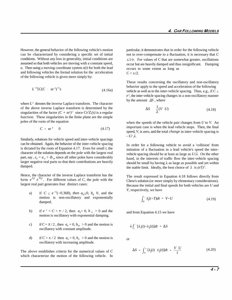
However, the general behavior of the following vehicle's motion particular, it demonstrates that in order for the following vehiclecan be characterized by considering a specific set of initialconditions. Without any loss in generality, initial conditions areassumed so that both vehicles are moving with a constant speed,u. Then using a moving coordinate system z(t) for both the leadand following vehicles the formal solution for the accelerationof the following vehicle is given more simply by:

(4.16a)

where L denotes the inverse Laplace transform. The character-1

of the above inverse Laplace transform is determined by thesingularities of the factor (C + se ) since Cs Z (s) is a regulars -1 2

5

function. These singularities in the finite plane are the simplepoles of the roots of the equation

Similarly, solutions for vehicle speed and inter-vehicle spacingscan be obtained. Again, the behavior of the inter-vehicle spacingis dictated by the roots of Equation 4.17. Even for small t, thecharacter of the solution depends on the pole with the largest realpart, say , s = a + ib , since all other poles have considerably0 0 0

larger negative real parts so that their contributions are heavilydamped.

Hence, the character of the inverse Laplace transform has theform . For different values of C, the pole with thelargest real part generates four distinct cases:

a) if , and themotion is non-oscillatory and exponentiallydamped.

b) if e < C < % / 2, then a < 0, b > 0 and the- 10 0

motion is oscillatory with exponential damping.

c) if C = % / 2 , then a = 0, b , > 0 and the motion is0 0

oscillatory with constant amplitude.

d) if C > % / 2 then a > 0, b > 0 and the motion is0 0

oscillatory with increasing amplitude.

The above establishes criteria for the numerical values of Cwhich characterize the motion of the following vehicle. In

not to over-compensate to a fluctuation, it is necessary that C

�1/e. For values of C that are somewhat greater, oscillationsoccur but are heavily damped and thus insignificant. Dampingoccurs to some extent as long as C < %/2.

These results concerning the oscillatory and non-oscillatorybehavior apply to the speed and acceleration of the following vehicle as well as to the inter-vehicle spacing. Thus, e.g., if C �e , the inter-vehicle spacing changes in a non-oscillatory manner-1

by the amount �S , where

when the speeds of the vehicle pair changes from U to V. Animportant case is when the lead vehicle stops. Then, the finalspeed, V, is zero, and the total change in inter-vehicle spacing is- U/ �. In order for a following vehicle to avoid a 'collision' frominitiation of a fluctuation in a lead vehicle's speed the inter-vehicle spacing should be at least as large as U/�. On the otherhand, in the interests of traffic flow the inter-vehicle spacingshould be small by having � as large as possible and yet withinthe stable limit. Ideally, the best choice of � is (eT) . -1

The result expressed in Equation 4.18 follows directly fromChow's solution (or more simply by elementary considerations).Because the initial and final speeds for both vehicles are U andV, respectively, we have

and from Equation 4.15 we have

or

�� &$5 )2//2:,1*02'(/6

� � �

as given earlier in Equation 4.18.

In order to illustrate the general theory of local stability, theresults of several calculations using a Berkeley Ease analogcomputer and an IBM digital computer are described. It isinteresting to note that in solving the linear car followingequation for two vehicles, estimates for the local stabilitycondition were first obtained using an analog computer fordifferent values of C which differentiate the various type ofmotion.

Figure 4.2 illustrates the solutions for C= e , where the lead-1

vehicle reduces its speed and then accelerates back to its originalspeed. Since C has a value for the locally stable limit, theacceleration and speed of the following vehicle, as well as theinter-vehicle spacing between the two vehicles are non-oscillatory.

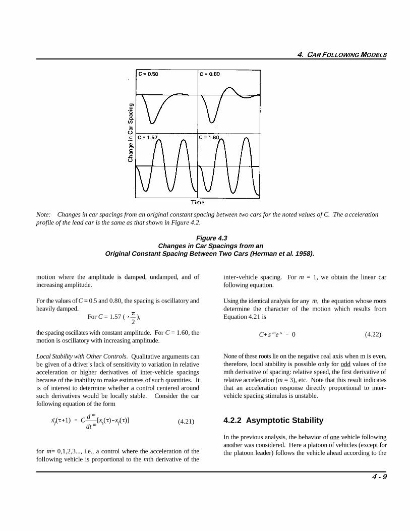
In Figure 4.3, the inter-vehicle spacing is shown for four othervalues of C for the same fluctuation of the lead vehicle as shownin Figure 4.2. The values of C range over the cases of oscillatory

Note: Vehicle 2 follows Vehicle 1 (lead car) with a time lag T=1.5 sec and a value of C=e (�0.368), the limiting value for local-1

stability. The initial velocity of each vehicle is u

Figure 4.2Detailed Motion of Two Cars Showing the

Effect of a Fluctuation in the Acceleration of the Lead Car (Herman et al. 1958).

xf(-�1) C d m

dt m[x

5(-)xf(-)]

C�s me s 0

�%

2

�� &$5 )2//2:,1*02'(/6

� � �

(4.21)

(4.22)

Note: Changes in car spacings from an original constant spacing between two cars for the noted values of C. The accelerationprofile of the lead car is the same as that shown in Figure 4.2.

Figure 4.3Changes in Car Spacings from an

Original Constant Spacing Between Two Cars (Herman et al. 1958).

motion where the amplitude is damped, undamped, and ofincreasing amplitude.

For the values of C = 0.5 and 0.80, the spacing is oscillatory andheavily damped.

For C = 1.57 ( ), Equation 4.21 is

the spacing oscillates with constant amplitude. For C = 1.60, themotion is oscillatory with increasing amplitude.

Local Stability with Other Controls. Qualitative arguments canbe given of a driver's lack of sensitivity to variation in relativeacceleration or higher derivatives of inter-vehicle spacingsbecause of the inability to make estimates of such quantities. Itis of interest to determine whether a control centered aroundsuch derivatives would be locally stable. Consider the carfollowing equation of the form

for m= 0,1,2,3..., i.e., a control where the acceleration of thefollowing vehicle is proportional to the mth derivative of the

inter-vehicle spacing. For m = 1, we obtain the linear carfollowing equation.

Using the identical analysis for any m, the equation whose rootsdetermine the character of the motion which results from

None of these roots lie on the negative real axis when m is even,therefore, local stability is possible only for odd values of themth derivative of spacing: relative speed, the first derivative ofrelative acceleration (m = 3), etc. Note that this result indicatesthat an acceleration response directly proportional to inter-vehicle spacing stimulus is unstable.

4.2.2 Asymptotic Stability

In the previous analysis, the behavior of one vehicle followinganother was considered. Here a platoon of vehicles (except forthe platoon leader) follows the vehicle ahead according to the

xn�1(t�T) �[ �xn(t) �xn�1(t)]

uo(t) ao� foei7t

un(t) ao� fnei7t

un(t) ao�F(7,�,,,n)ei6(7,�,,,n)

[1�(7�

)2�2(7

�)sin(7,)]n/2

1�(7�

)2�2(7

�)sin(7,) > 1

7

�> 2sin(7,)

�, < 12

[lim7�0(7,)/sin(7,)]

xn�1(t)�u0(t)4%n�

12�

T½

# exp [tn/�]4n/�(1/2�,)

�� &$5 )2//2:,1*02'(/6

� � ��

(4.23)

(4.24)

(4.25)

(4.26)

(4.27)

(4.28)

linear car following equation, Equation 4.15. The criterianecessary for asymptotic stability or instability were firstinvestigated by considering the Fourier components of the speedfluctuation of a platoon leader (Chandler et al. 1958).

The set of equations which attempts to describe a line of N i.e. ifidentical car-driver units is:

where n =0,1,2,3,...N.

Any specific solution to these equations depends on the velocityprofile of the lead vehicle of the platoon, u (t), and the two0

parameters � and T. For any inter-vehicle spacing, if adisturbance grows in amplitude then a 'collision' wouldeventually occur somewhere back in the line of vehicles.

While numerical solutions to Equation 4.23 can determine atwhat point such an event would occur, the interest is todetermine criteria for the growth or decay of such a disturbance.Since an arbitrary speed pattern can be expressed as a linearcombination of monochromatic components by Fourier analysis,the specific profile of a platoon leader can be simply representedby one component, i.e., by a constant together with amonochromatic oscillation with frequency, 7 and amplitude, fo

, i.e.,

and the speed profile of the nth vehicle by

Substitution of Equations 4.24 and 4.25 into Equation 4.23yields:

where the amplitude factor F (7, �, ,, n) is given by

which decreases with increasing n if

The severest restriction on the parameter � arises from the lowfrequency range, since in the limit as 7 � 0, � must satisfy theinequality

Accordingly, asymptotic stability is insured for all frequencieswhere this inequality is satisfied.

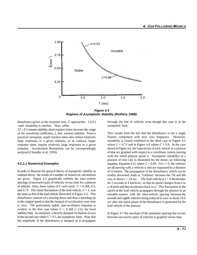
For those values of 7 within the physically realizable frequencyrange of vehicular speed oscillations, the right hand side of theinequality of 4.27 has a short range of values of 0.50 to about0.52. The asymptotic stability criteria divides the two parameterdomain into stable and unstable regions, as graphicallyillustrated in Figure 4.4.

The criteria for local stability (namely that no local oscillationsoccur when �,� e ) also insures asymptoticstability. It has also-1

been shown (Chandler et al. 1958) that a speed fluctuation canbe approximated by:

Hence, the speed of propagation of the disturbance with respectto the moving traffic stream in number of inter-vehicleseparations per second, n/t, is �.

That is, the time required for the disturbance to propagatebetween pairs of vehicles is � , a constant, which is independent-1

of the response time T. It is noted from the above equation thatin the propagation of a speed fluctuation the amplitude of the

c=0.52

Unstable

Stable

1.00

0.75

0.50

0.25

0 0.5 1.0 1.5 2.0

T (sec)

c=0.50

�� &$5 )2//2:,1*02'(/6

� � ��

Figure 4.4Regions of Asymptotic Stability (Rothery 1968).

disturbance grows as the response time, T, approaches 1/(2�) until instability is reached. Thus, while�T < 0.5 ensures stability, short reaction times increase the rangeof the sensitivity coefficient, �, that ensures stability. From apractical viewpoint, small reaction times also reduce relativelylarge responses to a given stimulus, or in contrast, largerresponse times require relatively large responses to a givenstimulus. Acceleration fluctuations can be correspondinglyanalyzed (Chandler et al. 1958).

4.2.1.1 Numerical Examples

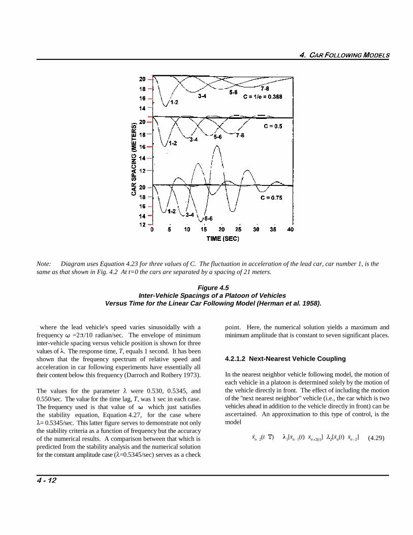
In order to illustrate the general theory of asymptotic stability asoutlined above, the results of a number of numerical calculationsare given. Figure 4.5 graphically exhibits the inter-vehiclespacings of successive pairs of vehicles versus time for a platoonof vehicles. Here, three values of C were used: C = 0.368, 0.5,and 0.75. The initial fluctuation of the lead vehicle, n = 1, wasthe same as that of the lead vehicle illustrated in Figure 4.2. Thisdisturbance consists of a slowing down and then a speeding upto the original speed so that the integral of acceleration over timeis zero. The particularly stable, non-oscillatory response isevident in the first case where C = 0.368 (�1/e), the localstability limit. As analyzed, a heavily damped oscillation occursin the second case where C = 0.5, the asymptotic limit. Note thatthe amplitude of the disturbance is damped as it propagates

through the line of vehicles even though this case is at theasymptotic limit.

This results from the fact that the disturbance is not a singleFourier component with near zero frequency. However,instability is clearly exhibited in the third case of Figure 4.5where C = 0.75 and in Figure 4.6 where C = 0.8. In the caseshown in Figure 4.6, the trajectories of each vehicle in a platoonof nine are graphed with respect to a coordinate system movingwith the initial platoon speed u. Asymptotic instability of aplatoon of nine cars is illustrated for the linear car followingequation, Equation 4.23, where C = 0.80. For t = 0, the vehiclesare all moving with a velocity u and are separated by a distanceof 12 meters. The propagation of the disturbance, which can bereadily discerned, leads to "collision" between the 7th and 8thcars at about t = 24 sec. The lead vehicle at t = 0 deceleratesfor 2 seconds at 4 km/h/sec, so that its speed changes from u tou -8 km/h and then accelerates back to u. This fluctuation in thespeed of the lead vehicle propagates through the platoon in anunstable manner with the inter-vehicle spacing between theseventh and eighth vehicles being reduced to zero at about 24.0sec after the initial phase of the disturbance is generated by thelead vehicle of the platoon.

In Figure 4.7 the envelope of the minimum spacing that occursbetween successive pairs of vehicles is graphed versus time

xn�2(t�,) �1[ �xn�1(t) �xn�2(t)]��2[ �xn(t) �xn�2]

�� &$5 )2//2:,1*02'(/6

� � ��

(4.29)

Note: Diagram uses Equation 4.23 for three values of C. The fluctuation in acceleration of the lead car, car number 1, is thesame as that shown in Fig. 4.2 At t=0 the cars are separated by a spacing of 21 meters.

Figure 4.5Inter-Vehicle Spacings of a Platoon of Vehicles

Versus Time for the Linear Car Following Model (Herman et al. 1958).

where the lead vehicle's speed varies sinusoidally with a point. Here, the numerical solution yields a maximum andfrequency 7 =2%/10 radian/sec. The envelope of minimum minimum amplitude that is constant to seven significant places.inter-vehicle spacing versus vehicle position is shown for threevalues of �. The response time, T, equals 1 second. It has beenshown that the frequency spectrum of relative speed andacceleration in car following experiments have essentially alltheir content below this frequency (Darroch and Rothery 1973).

The values for the parameter � were 0.530, 0.5345, and0.550/sec. The value for the time lag, T, was 1 sec in each case.The frequency used is that value of 7 which just satisfiesthe stability equation, Equation 4.27, for the case where�= 0.5345/sec. This latter figure serves to demonstrate not onlythe stability criteria as a function of frequency but the accuracyof the numerical results. A comparison between that which ispredicted from the stability analysis and the numerical solutionfor the constant amplitude case (�=0.5345/sec) serves as a check

4.2.1.2 Next-Nearest Vehicle Coupling

In the nearest neighbor vehicle following model, the motion ofeach vehicle in a platoon is determined solely by the motion ofthe vehicle directly in front. The effect of including the motionof the "next nearest neighbor" vehicle (i.e., the car which is twovehicles ahead in addition to the vehicle directly in front) can beascertained. An approximation to this type of control, is themodel

�� &$5 )2//2:,1*02'(/6

� � ��

Note: Diagram illustrates the linear car following equation, eq. 4.23, where C=080.

Figure 4.6Asymptotic Instability of a Platoon of Nine Cars (Herman et al. 1958).

Figure 4.7Envelope of Minimum Inter-Vehicle Spacing Versus Vehicle Position (Rothery 1968 ).

(�1��2), < 12

(7,)/sin(7,)] (�1��2), > 12

xn�1(t�,) �[ �xn(t) �xn�1(t)]

Sf Si��1(Uf Ui)

k1f k1

i ��1(UfUi)

�� &$5 )2//2:,1*02'(/6

� � ��

(4.30) (4.31)

(4.32)

(4.33)

(4.34)

which in the limit 7� 0 is This equation states that the effect of adding next nearestneighbor coupling to the control element is, to the first order, toincrease � to (� + � ). This reduces the value that � can have1 1 2 1

and still maintain asymptotic stability.

4.3 Steady-State Flow

This section discusses the properties of steady-state traffic flow also follows from elementary considerations by integration ofbased on car following models of single-lane traffic flow. In Equation 4.32 as shown in the previous section (Gazis et al.particular, the associated speed-spacing or equivalent speed-concentration relationships, as well as the flow-concentrationrelationships for single lane traffic flow are developed.

The Linear Case. The equations of motion for a single lane oftraffic described by the linear car following model are given by:

where n = 1, 2, 3, ....

In order to interrelate one steady-state to another under thiscontrol, assume (up to a time t=0) each vehicle is traveling at a 1) They link an initial steady-state to a second arbitraryspeed U and that the inter-vehicle spacing is S . Suppose thati i

at t=0, the lead vehicle undergoes a speed change and increasesor decreases its speed so that its final speed after some time, t, isU . A specific numerical solution of this type of transition isf

exhibited in Figure 4.8.

In this example C = �T=0.47 so that the stream of traffic isstable, and speed fluctuations are damped. Any case where theasymptotic stability criteria is satisfied assures that eachfollowing vehicle comprising the traffic stream eventuallyreaches a state traveling at the speed U . In the transition fromf

a speed U to a speed U , the inter-vehicle spacing S changesi f

from S to S , wherei f

This result follows directly from the solution to the car followingequation, Equation 4.16a or from Chow (1958). Equation 4.33

1959). This result is not directly dependent on the time lag, T,except that for this result to be valid the time lag, T, must allowthe equation of motion to form a stable stream of traffic. Sincevehicle spacing is the inverse of traffic stream concentration, k,the speed-concentration relation corresponding to Equation 4.33is:

The significance of Equations 4.33 and 4.34 is that:

steady-state, and

2) They establish relationships between macroscopic trafficstream variables involving a microscopic car followingparameter, � .

In this respect they can be used to test the applicability of the carfollowing model in describing the overall properties of singlelane traffic flow. For stopped traffic, U = 0, and thei

corresponding spacing, S , is composed of vehicle length ando

"bumper-to-bumper" inter-vehicle spacing. The concentrationcorresponding to a spacing, S, is denoted by k and is frequentlyo j

referred to as the 'jam concentration'.

Given k, then Equation 4.34 for an arbitrary traffic state definedj

by a speed, U, and a concentration, k, becomes

U �(k1k1

j )

q Uk �(1 kkj

)

�� &$5 )2//2:,1*02'(/6

� � ��

(4.35)

(4.36)

Note: A numerical solution to Equation 4.32 for the inter-vehicle spacings of an 11- vehicle platoon going from one steady-state toanother (�T = 0.47). The lead vehicle's speed decreases by 7.5 meters per second.

Figure 4.8Inter-Vehicle Spacings of an Eleven Vehicle Platoon (Rothery 1968).

A comparison of this relationship was made (Gazis et al. 1959)with a specific set of reported observations (Greenberg 1959) fora case of single lane traffic flow (i.e., for the northbound trafficflowing through the Lincoln Tunnel which passes under the The inability of Equation 4.36 to exhibit the required qualitativeHudson River between the States of New York and New Jersey). relationship between flow and concentration (see Chapter 2) ledThis comparison is reproduced in Figure 4.9 and leads to an to the modification of the linear car following equation (Gazis etestimate of 0.60 sec for �. This estimate of � implies an upper al. 1959).-1

bound for T � 0.83 sec for an asymptotic stable traffic streamusing this facility.

While this fit and these values are not unreasonable, afundamental problem is identified with this form of an equationfor a speed-spacing relationship (Gazis et al. 1959). Because itis linear, this relationship does not lead to a reasonabledescription of traffic flow. This is illustrated in Figure 4.10where the same data from the Lincoln Tunnel (in Figure 4.9) isregraphed. Here the graph is in the form of a normalized flow,

versus a normalized concentration together with thecorresponding theoretical steady-state result derived fromEquation 4.35, i.e.,

Non-Linear Models. The linear car following model specifiesan acceleration response which is completely independent ofvehicle spacing (i.e., for a given relative velocity, response is thesame whether the vehicle following distance is small [e.g., of theorder of 5 or 10 meters] or if the spacing is relatively large [i.e.,of the order of hundreds of meters]). Qualitatively, we wouldexpect that response to a given relative speed to increase withsmaller spacings.

�� &$5 )2//2:,1*02'(/6

� � ��

Note: The data are those of (Greenberg 1959) for the Lincoln Tunnel. The curve represents a "least squares fit" of Equation 4.35to the data.

Figure 4.9Speed (miles/hour) Versus Vehicle Concentration (vehicles/mile).(Gazis et al. 1959).

Note: The curve corresponds to Equation 4.36 where the parameters are those from the "fit" shown in Figure 4.9.

Figure 4.10Normalized Flow Versus Normalized Concentration (Gazis et al. 1959).

� �1/S(t) �1/[xn(t)xn�1(t)]

xn�1(t�,) �1

[xn(t)xn�1(t)][ �xn(t) �xn�1(t)]

u �1ln (kj /k)

q �1kln(kj /k)

�� &$5 )2//2:,1*02'(/6

� � ��

(4.37)

(4.38)

(4.39)

(4.40)

In order to attempt to take this effect into account, the linear therefore the flow-concentration relationship, does not describemodel is modified by supposing that the gain factor, �, is not a the state of the traffic stream. constant but is inversely proportional to vehicle spacing, i.e.,

where � is a new parameter - assumed to be a constant and approaches to single-lane traffic flow because in these cases any1

which shall be referred to as the sensitivity coefficient. Using small speed change, once the disturbance arrives, each vehicleEquation 4.37 in Equation 4.32, our car following equation is: instantaneously relaxes to the new speed, at the 'proper' spacing.

for n = 1,2,3,... downstream from the vehicle initiating the speed change at a

As before, by assuming the parameters are such that the trafficstream is stable, this equation can be integrated yielding thesteady-state relation for speed and concentration:

and for steady-state flow and concentration:

where again it is assumed that for u=0, the spacing is equal toan effective vehicle length, L = k . These relations for steady--1

state flow are identical to those obtained from considering thetraffic stream to be approximated by a continuous compressiblefluid (see Chapter 5) with the property that disturbances arepropagated with a constant speed with respect to the movingmedium (Greenberg 1959). For our non-linear car followingequation, infinitesimal disturbances are propagated with speed� . This is consistent with the earlier discussion regarding the1

speed of propagation of a disturbance per vehicle pair.

It can be shown that if the propagation time, , , is directly0

proportional to spacing (i.e., , � S), Equations 4.39 and 4.400

are obtained where the constant ratio S /, is identified as the Assuming that this data is a representative sample of thiso

constant � . facility's traffic, the value of 27.7 km/h is an estimate not only ofl

These two approaches are not analogous. In the fluid analogy but it is the 'characteristic speed' for the roadway undercase, the speed-spacing relationship is 'followed' at every instant consideration (i.e., the speed of the traffic stream whichbefore, during, and after a disturbance. In the case of car maximizes the flow). following during the transition phase, the speed-spacing, and

A solution to any particular set of equations for the motion of atraffic stream specifies departures from the steady-state. This isnot the case for simple headway models or hydro-dynamical

This emphasizes the shortcoming of these alternate approaches.They cannot take into account the behavioral and physicalaspects of disturbances. In the case of car following models, theinitial phase of a disturbance arrives at the nth vehicle

time (n-1)T seconds after the onset of the fluctuation. The timeit takes vehicles to reach the changed speed depends on theparameter �, for the linear model, and � , for the non-linear1

model, subject to the restriction that � > T or � < S/T,-11

respectively.

These restrictions assure that the signal speed can never precedethe initial phase speed of a disturbance. For the linear case, therestriction is more than satisfied for an asymptotic stable traffic stream. For small speed changes, it is also satisfied for the non-linear model by assuming that the stability criteria results for thelinear case yields a bound for the stability in the non-linear case. Hence, the inequality �, /S*<0.5 provides a sufficient stabilitycondition for the non-linear case, where S* is the minimumspacing occurring during a transition from one steady-state toanother.

Before discussing a more general form for the sensitivitycoefficient (i.e., Equation 4.37), the same reported data(Greenberg 1959) plotted in Figures 4.9 and 4.10 are graphed inFigures 4.11 and 4.12 together with the steady-state relations(Equations 4.39 and 4.40 obtained from the non-linear model,Equation 4.38). The fit of the data to the steady-state relation viathe method of "least squares" is good and the resulting values for� and k are 27.7 km/h and 142 veh/km, respectively.1 j

the sensitivity coefficient for the non-linear car following model

�� &$5 )2//2:,1*02'(/6

� � ��

Note: The curve corresponds to a "least squares" fit of Equation 4.39 to the data (Greenberg 1959).

Figure 4.11Speed Versus Vehicle Concentration (Gazis et al. 1959).

Note: The curve corresponds to Equation 4.40 where parameters are those from the "fit" obtained in Figure 4.11.

Figure 4.12Normalized Flow Versus Normalized Vehicle Concentration (Edie et al. 1963).

� �2x.n�1(t�,)/[xn(t)xn�1(t)]

2

xn�1(t�,)�2x

.n�1(t�,)

[xn(t)xn�1(t)]2[x.

n(t)x.n�1(t)]

U Uf ek/km

q Uf kek/km

U Uf for 0�k�kf

U Uf expk kf

km

U Uf (1k/kj)

U Uf (1L/S)

�U (Uf L/S2) �S

xn�1(t�,) Uf L

[xn(t)xn�1(t)]2[ �xn(t) �xn�1(t)]

�� &$5 )2//2:,1*02'(/6

� � ��

(4.41)

(4.42)

(4.43)

(4.44)

(4.45)

(4.46)

(4.47)

(4.48)

(4.49)

The corresponding vehicle concentration at maximum flow, i.e.,when u = � , is e k. This predicts a roadway capacity of1 j

-l

� e k of about �1400 veh/h for the Lincoln Tunnel. A noted1 j-l

undesirable property of Equation 4.40 is that the tangent dq/dtis infinite at k = 0, whereas a linear relation between flow andconcentration would more accurately describe traffic near zeroconcentration. This is not a serious defect in the model since carfollowing models are not applicable for low concentrationswhere spacings are large and the coupling between vehicles areweak. However, this property of the model did suggest thefollowing alternative form (Edie 1961) for the gain factor,

This leads to the following expression for a car following model:

As before, this can be integrated giving the following steady-state equations:

and

where U is the "free mean speed", i.e., the speed of the trafficf

stream near zero concentration and k is the concentration whenm

the flow is a maximum. In this case the sensitivity coefficient, �2

can be identified as k . The speed at optimal flow is e Um f-1 -1

which, as before, corresponds to the speed of propagation of adisturbance with respect to the moving traffic stream. Thismodel predicts a finite speed, U , near zero concentration. f

Ideally, this speed concentration relation should be translated tothe right in order to more completely take into accountobservations that the speed of the traffic stream is independentof vehicle concentration for low concentrations, .i.e.

and

where k corresponds to a concentration where vehicle tof

vehicle interactions begin to take place so that the stream speedbegins to decrease with increasing concentration. Assuming thatinteractions take place at a spacing of about 120 m, k wouldf

have a value of about 8 veh/km. A "kink" of this kind wasintroduced into a linear model for the speed concentrationrelationship (Greenshields 1935).

Greenshields' empirical model for a speed-concentration relationis given by

where U is a “free mean speed” and k is the jam concentration.f j

It is of interest to question what car following model wouldcorrespond to the above steady-state equations as expressed byEquation 4.46. The particular model can be derived in thefollowing elementary way (Gazis et al. 1961). Equation 4.46 isrewritten as

Differentiating both sides with respect to time obtains

which after introduction of a time lag is for the (n+1) vehicle:

Uf L

[xn(t)xn�1(t)]2

xn�1(t�,) �[ �xn(t) �xn�1(t)]

� a5,m�x m

n�1(t�,)/[xn(t)xn�1(t)]5

fm(U) a # fl(S)�b

fp(x) x1p

fp(x) 5nx

b fm(Uf )

b afl(L)

�� &$5 )2//2:,1*02'(/6

� � ��

(4.50)

(4.51)

(4.52)

(4.53)

(4.54)

(4.55)

(4.56)

(4.57)

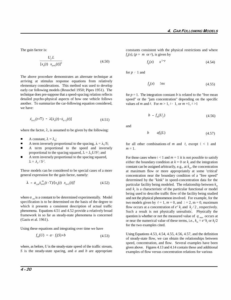
The gain factor is:

The above procedure demonstrates an alternate technique atarriving at stimulus response equations from relativelyelementary considerations. This method was used to developearly car following models (Reuschel 1950; Pipes 1951). Thetechnique does pre-suppose that a speed-spacing relation reflectsdetailed psycho-physical aspects of how one vehicle followsanother. To summarize the car-following equation considered,we have:

where the factor, �, is assumed to be given by the following:

� A constant, � = � ;0

� A term inversely proportional to the spacing, � = � /S; 1

� A term proportional to the speed and inverselyproportional to the spacing squared, � = � U/S ; and2

2

� A term inversely proportional to the spacing squared, � = � / S .3

2

These models can be considered to be special cases of a moregeneral expression for the gain factor, namely:

where a is a constant to be determined experimentally. Model 5,m

specification is to be determined on the basis of the degree towhich it presents a consistent description of actual trafficphenomena. Equations 4.51 and 4.52 provide a relatively broadframework in so far as steady-state phenomena is concerned(Gazis et al. 1961).

Using these equations and integrating over time we have

where, as before, U is the steady-state speed of the traffic stream,S is the steady-state spacing, and a and b are appropriate

constants consistent with the physical restrictions and wheref (x), (p = m or 5), is given by p

for p g 1 and

for p = 1. The integration constant b is related to the "free meanspeed" or the "jam concentration" depending on the specificvalues of m and 5. For m > 1, 5g 1, or m =1, 5 >1

and

for all other combinations of m and 5, except 5 < 1 and m = 1.

For those cases where 5 < 1 and m = 1 it is not possible to satisfyeither the boundary condition at k = 0 or k and the integrationj

constant can be assigned arbitrarily, e.g., at k , the concentrationm

at maximum flow or more appropriately at some 'critical'concentration near the boundary condition of a "free speed"determined by the "kink" in speed-concentration data for theparticular facility being modeled. The relationship between km

and k is a characteristic of the particular functional or modelj

being used to describe traffic flow of the facility being studiedand not the physical phenomenon involved. For example, for thetwo models given by 5 = 1, m = 0, and 5 = 2, m = 0, maximumflow occurs at a concentration of e k and k / 2 , respectively.-l

j j

Such a result is not physically unrealistic. Physically thequestion is whether or not the measured value of q occurs atmax

or near the numerical value of these terms, i.e., k = e k or k /2m j j-1

for the two examples cited.

Using Equations 4.53, 4.54, 4.55, 4.56, 4.57, and the definitionof steady-state flow, we can obtain the relationships betweenspeed, concentration, and flow. Several examples have beengiven above. Figures 4.13 and 4.14 contain these and additionalexamples of flow versus concentration relations for various

�� &$5 )2//2:,1*02'(/6

� � ��

Note: Normalized flow versus normalized concentration corresponding to the steady-state solution of Equations 4.51 and 4.52for m=1 and various values of 5.

Figure 4.13Normalized Flow Versus Normalized Concentration (Gazis et al. 1963).

Figure 4.14Normalized Flow versus Normalized Concentration Corresponding to the Steady-State

Solution of Equations 4.51 and 4.52 for m=1 and Various Values of 55 (Gazis 1963).

�� &$5 )2//2:,1*02'(/6

� � ��

values of 5 and m. These flow curves are normalized by lettingq = q/q , and k = k/k .n max n j

It can be seen from these figures that most of the models shownhere reflect the general type of flow diagram required to agreewith the qualitative descriptions of steady-state flow. Thespectrum of models provided are capable of fitting data like thatshown in Figure 4.9 so long as a suitable choice of theparameters is made. spacing, i.e., m= 0, 5 =1 (Herman et al. 1959). A generalized

equation for steady-state flow (Drew 1965) and subsequentlyThe generalized expression for car following models, Equations tested on the Gulf Freeway in Houston, Texas led to a model4.51 and 4.52, has also been examined for non-integral valuesfor m and 5 (May and Keller 1967). Fittingdata obtained on theEisenhower Expressway in Chicago they proposed a model with As noted earlier, consideration of a "free-speed" near lowm = 0.8 and 5 = 2.8. Various values for m and 5 can be identifiedin the early work on steady-state flow and car following . model m = 1, 5 = 2 (Edie 1961). Yet another model, m = 1,

The case m = 0, 5 = 0 equates to the "simple" linear car followingmodel. The case m = 0, 5 = 2 can be identified with a modeldeveloped from photographic observations of traffic flow madein 1934 (Greenshields 1935). This model can also be developed

considering the perceptual factors that are related to the carfollowing task (Pipes and Wojcik 1968; Fox and Lehman 1967;Michaels 1963). As was discussed earlier, the case for m = 0,5 = 1 generates a steady-state relation that can be developed byafluid flow analogy to traffic (Greenberg 1959) and led to thereexamination of car following experiments and the hypothesisthat drivers do not have a constant gain factor to a given relative-speed stimulus but rather that it varies inversely with the vehicle

where m = 0 and 5 = 3/2.

concentrations led to the proposal and subsequent testing of the

5 = 3 resulted from analysis of data obtained on the EisenhowerExpressway in Chicago (Drake et al. 1967). Further analysis ofthis model together with observations suggest that the sensitivitycoefficient may take on different values above a lane flow ofabout 1,800 vehicles/hr (May and Keller 1967).

4.4 Experiments And Observations

This section is devoted to the presentation and discussion of derived from car following models for steady-state flow areexperiments that have been carried out in an effort to ascertain examined. whether car following models approximate single lane trafficcharacteristics. These experiments are organized into two Finally, the degree to which any specific model of the typedistinct categories. examined in the previous section is capable of representing a

The first of these is concerned with comparisons between car macroscopic viewpoints is examined. following models and detailed measurements of the variablesinvolved in the driving situation where one vehicle followsanother on an empty roadway. These comparisons lead to aquantitative measure of car following model estimates for thespecific parameters involved for the traffic facility and vehicletype used.

The second category of experiments are those concerned withthe measurement of macroscopic flow characteristics: the studyof speed, concentration, flow and their inter-relationships forvehicle platoons and traffic environments where traffic ischanneled in a single lane. In particular, the degree to which thistype of data fits the analytical relationships that have been

consistent framework from both the microscopic and

4.4.1 Car Following Experiments

The first experiments which attempted to make a preliminaryevaluation of the linear car following model were performed anumber of decades ago (Chandler et al. 1958; Kometani andSasaki 1958). In subsequent years a number of different testswith varying objectives were performed using two vehicles,three vehicles, and buses. Most of these tests were conducted ontest track facilities and in vehicular tunnels.

xn�1(t�,) �[ �xn(t) �xn�1(t)]��xn(t)

�� &$5 )2//2:,1*02'(/6

� � ��

(4.58)

In these experiments, inter-vehicle spacing, relative speed, speedof the following vehicle, and acceleration of the followingvehicles were recorded simultaneously together with a clocksignal to assure synchronization of each variable with everyother.

These car following experiments are divided into six specificcategories as follows:

1) Preliminary Test Track Experiments. The firstexperiments in car following were performed by (Chandleret al. 1958) and were carried out in order to obtainestimates of the parameters in the linear car followingmodel and to obtain a preliminary evaluation of this model.Eight male drivers participated in the study which wasconducted on a one-mile test track facility.

2) Vehicular Tunnel Experiments. To further establish the even though the relative speed has been reduced to zero orvalidity of car following models and to establish estimates, near zero. This situation was observed in several cases inthe parameters involved in real operating environments tests carried out in the vehicular tunnels - particularlywhere the traffic flow characteristics were well known, a when vehicles were coming to a stop. Equation 4.58series of experiments were carried out in the Lincoln, above allows for a non-zero acceleration when the relativeHolland, and Queens Mid-Town Tunnels of New York speed is zero. A value of � near one would indicate anCity. Ten different drivers were used in collecting 30 test attempt to nearly match the acceleration of the lead driverruns. for such cases. This does not imply that drivers are good

3) Bus Following Experiments. A series of experimentswere performed to determine whether the dynamicalcharacteristics of a traffic stream changes when it iscomposed of vehicles whose performance measures aresignificantly different than those of an automobile. Theywere also performed to determine the validity and measureparameters of car following models when applied to heavyvehicles. Using a 4 kilometer test track facility and 53-passenger city buses, 22 drivers were studied. b) Experiments of Forbes et al. Several experiments

4) Three Car Experiments. A series of experiments wereperformed to determine the effect on driver behavior whenthere is an opportunity for next-nearest following and offollowing the vehicle directly ahead. The degree to whicha driver uses the information that might be obtained froma vehicle two ahead was also examined. The relativespacings and the relative speeds between the first and thirdvehicles and the second and third vehicles together withthe speed and acceleration of the third vehicle wererecorded.

5) Miscellaneous Experiments. Several additional carfollowing experiments have been performed and reportedon as follows:

a) Kometani and Sasaki Experiments. Kometani andSasaki conducted and reported on a series of experimentsthat were performed to evaluate the effect of an additionalterm in the linear car following equation. This term isrelated to the acceleration of the lead vehicle. Inparticular, they investigated a model rewritten here in thefollowing form:

This equation attempts to take into account a particulardriving phenomenon, where the driver in a particular staterealizes that he should maintain a non-zero acceleration

estimators of relative acceleration. The conjecture here isthat by pursuing the task where the lead driver isundergoing a constant or near constant accelerationmaneuver, the driver becomes aware of this qualitativelyafter nullifying out relative speed - and thereby shifts theframe of reference. Such cases have been incorporatedinto models simulating the behavior of bottlenecks intunnel traffic (Helly 1959).

using three vehicle platoons were reported by Forbes et al. (1957). Here a lead vehicle was driven by one of theexperimenters while the second and third vehicles weredriven by subjects. At predetermined locations along theroadway relatively severe acceleration maneuvers wereexecuted by the lead vehicle. Photographic equipmentrecorded these events with respect to this movingreference together with speed and time. From theserecordings speeds and spacings were calculated as afunction of time. These investigators did not fit this datato car following models. However, a partial set of this datawas fitted to vehicle following models by anotherinvestigator (Helly 1959). This latter set consisted of six

�� &$5 )2//2:,1*02'(/6

� � ��

tests in all, four in the Lincoln Tunnel and two on an for which the correlation coefficient is a maximum and typicallyopen roadway. falls in the range of 0.85 to 0.95.

c) Ohio State Experiments. Two different sets ofexperiments have been conducted at Ohio StateUniversity. In the first set a series of subjects have been given for �, their product; C = �T, the boundary value forstudied using a car following simulator (Todosiev 1963).An integral part of the simulator is an analog computerwhich could program the lead vehicle for many differentdriving tasks. The computer could also simulate theperformance characteristics of different following vehicles.These experiments were directed toward understanding themanner in which the following vehicle behaves when thelead vehicle moves with constant speed and themeasurement of driver thresholds for changes in spacing,relative speed, and acceleration. The second set ofexperiments were conducted on a level two-lane statehighway operating at low traffic concentrations (Hankinand Rockwell 1967). In these experiments the purposewas "to develop an empirically based model of carfollowing which would predict a following car'sacceleration and change in acceleration as a function ofobserved dynamic relationships with the lead car." As inthe earlier car following experiments, spacing and relativespeed were recorded as well as speed and acceleration ofthe following vehicle.

d) Studies by Constantine and Young. These studieswere carried out using motorists in England and aphotographic system to record the data (Constantine andYoung 1967). The experiments are interesting from thevantage point that they also incorporated a secondphotographic system mounted in the following vehicle anddirected to the rear so that two sets of car following datacould be obtained simultaneously. The latter set collectedinformation on an unsuspecting motorist. Althoughaccuracy is not sufficient, such a system holds promise.

4.4.1.1 Analysis of Car Following Experiments

The analysis of recorded information from a car followingexperiment is generally made by reducing the data to numericalvalues at equal time intervals. Then, a correlation analysis iscarried out using the linear car following model to obtainestimates of the two parameters, � and T. With the data indiscrete form, the time lag ,T, also takes on discrete values. Thetime lag or response time associated with a given driver is one

The results from the preliminary experiments (Chandler et al.1958) are summarized in Table 4.1 where the estimates are

asymptotic stability; average spacing, < S >; and average speed,< U >. The average value of the gain factor is 0.368 sec . The-1

average value of �T is close to 0.5, the asymptotic stabilityboundary limit.

Table 4.1 Results from Car-Following Experiment

Driver �� <U> <S> ��T

1 0.74 sec 19.8 36 1.04-1

m/sec m

2 0.44 16 36.7 0.44

3 0.34 20.5 38.1 1.52

4 0.32 22.2 34.8 0.48

5 0.38 16.8 26.7 0.65

6 0.17 18.1 61.1 0.19

7 0.32 18.1 55.7 0.72

8 0.23 18.7 43.1 0.47

Using the values for � and the average spacing <S > obtained foreach subject a value of 12.1 m/sec (44.1 km/h) is obtained for anestimate of the constant a (Herman and Potts 1959). This1, 0

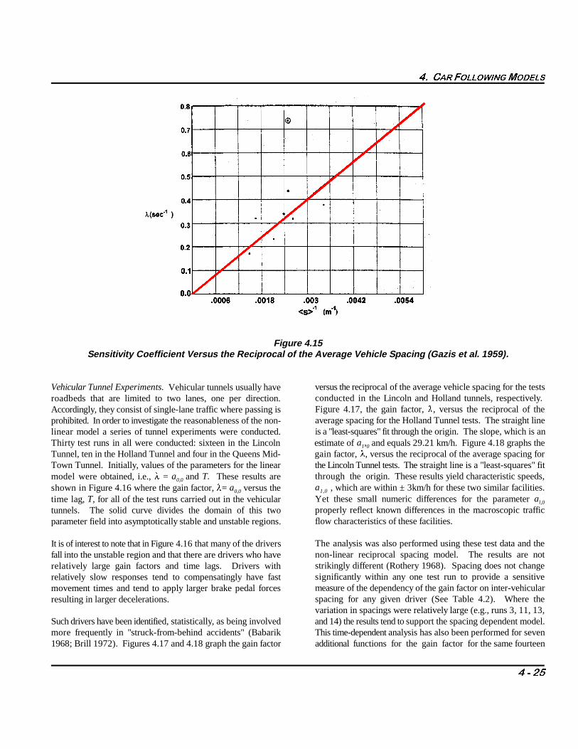
latter estimate compares the value � for each driver with thatdriver's average spacing, <S > , since each driver is in somewhatdifferent driving state. This is illustrated in Figure 4.15. Thisapproach attempts to take into account the differences in theestimates for the gain factor � or a , obtained for different0,0

drivers by attributing these differences to the differences in theirrespective average spacing. An alternate and more directapproach carries out the correlation analysis for this model usingan equation which is the discrete form of Equation 4.38 to obtaina direct estimate of the dependence of the gain factor on spacing,S(t).

�� &$5 )2//2:,1*02'(/6

� � ��

Figure 4.15Sensitivity Coefficient Versus the Reciprocal of the Average Vehicle Spacing (Gazis et al. 1959).

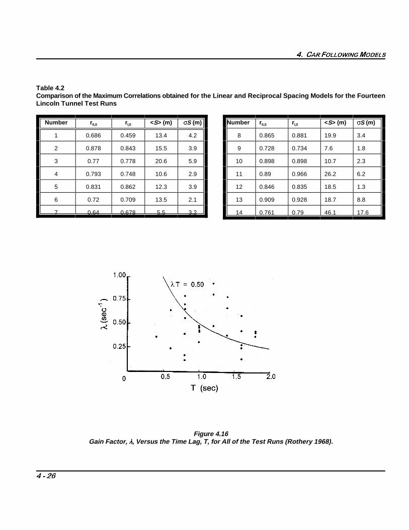
Vehicular Tunnel Experiments. Vehicular tunnels usually haveroadbeds that are limited to two lanes, one per direction.Accordingly, they consist of single-lane traffic where passing isprohibited. In order to investigate the reasonableness of the non-linear model a series of tunnel experiments were conducted.Thirty test runs in all were conducted: sixteen in the Lincoln estimate of a , and equals 29.21 km/h. Figure 4.18 graphs theTunnel, ten in the Holland Tunnel and four in the Queens Mid- gain factor, �, versus the reciprocal of the average spacing forTown Tunnel. Initially, values of the parameters for the linear the Lincoln Tunnel tests. The straight line is a "least-squares" fitmodel were obtained, i.e., � = a and T. These results are0,0

shown in Figure 4.16 where the gain factor, �= a versus the0,0

time lag, T, for all of the test runs carried out in the vehiculartunnels. The solid curve divides the domain of this twoparameter field into asymptotically stable and unstable regions.

It is of interest to note that in Figure 4.16 that many of the driversfall into the unstable region and that there are drivers who haverelatively large gain factors and time lags. Drivers withrelatively slow responses tend to compensatingly have fastmovement times and tend to apply larger brake pedal forcesresulting in larger decelerations.

Such drivers have been identified, statistically, as being involved and 14) the results tend to support the spacing dependent model.more frequently in "struck-from-behind accidents" (Babarik This time-dependent analysis has also been performed for seven1968; Brill 1972). Figures 4.17 and 4.18 graph the gain factor additional functions for the gain factor for the same fourteen

versus the reciprocal of the average vehicle spacing for the testsconducted in the Lincoln and Holland tunnels, respectively. Figure 4.17, the gain factor, �, versus the reciprocal of theaverage spacing for the Holland Tunnel tests. The straight lineis a "least-squares" fit through the origin. The slope, which is an

1 0

through the origin. These results yield characteristic speeds,a , which are within ± 3km/h for these two similar facilities.1,0

Yet these small numeric differences for the parameter al,0

properly reflect known differences in the macroscopic trafficflow characteristics of these facilities.

The analysis was also performed using these test data and thenon-linear reciprocal spacing model. The results are notstrikingly different (Rothery 1968). Spacing does not changesignificantly within any one test run to provide a sensitivemeasure of the dependency of the gain factor on inter-vehicularspacing for any given driver (See Table 4.2). Where thevariation in spacings were relatively large (e.g., runs 3, 11, 13,

�� &$5 )2//2:,1*02'(/6

� � ��

Table 4.2Comparison of the Maximum Correlations obtained for the Linear and Reciprocal Spacing Models for the FourteenLincoln Tunnel Test Runs

Number r r < S> (m) ))S (m) Number r r < S> (m) ))S (m)0,0 l,0

1 0.686 0.459 13.4 4.2 8 0.865 0.881 19.9 3.4

2 0.878 0.843 15.5 3.9 9 0.728 0.734 7.6 1.8

3 0.77 0.778 20.6 5.9 10 0.898 0.898 10.7 2.3

4 0.793 0.748 10.6 2.9 11 0.89 0.966 26.2 6.2

5 0.831 0.862 12.3 3.9 12 0.846 0.835 18.5 1.3

6 0.72 0.709 13.5 2.1 13 0.909 0.928 18.7 8.8

7 0.64 0.678 5.5 3.2 14 0.761 0.79 46.1 17.6

0,0 l,0

Figure 4.16Gain Factor, ��, Versus the Time Lag, T, for All of the Test Runs (Rothery 1968).

�� &$5 )2//2:,1*02'(/6

� � ��

Note: The straight line is a "least-squares" fit through the origin. The slope, which is an estimate of a , equals 29.21 km/h.1,0

Figure 4.17Gain Factor, ��, Versus the Reciprocal of the

Average Spacing for Holland Tunnel Tests (Herman and Potts 1959).

Note: The straight line is a "least-squares" fit through the origin. The slope, is an estimate of a , equals 32.68 km/h.1,0

Figure 4.18Gain Factor, �� ,Versus the Reciprocal of the

Average Spacing for Lincoln Tunnel Tests (Herman and Potts 1959).

�� &$5 )2//2:,1*02'(/6

� � ��

little difference from one model to the other. There are definite of the cases when that factor is introduced and this model (5=1;trends however. If one graphs the correlation coefficient for agiven 5, say 5=1 versus m; 13 of the cases indicate the best fits the analysis are summarized in Figure 4.19 where the sensitivityare with m = 0 or 1. Three models tend to indicate marginal coefficient a versus the time lag, T, for the bus followingsuperiority; they are those given by (5=2; m=1), (5=1; m=0) and(5=2; m=0).

Bus Following Experiments. For each of the 22 drivers tested,the time dependent correlation analysis was carried out for thelinear model (5=0; m=0), the reciprocal spacing model (5=1;m=0), and the speed, reciprocal-spacing-squared model (5=2;m=1). Results similar to the Tunnel analysis were obtained: highcorrelations for almost all drivers and for each of the threemodels examined (Rothery et al. 1964).

The correlation analysis provided evidence for the reciprocalspacing effect with the correlation improved in about 75 percent

m=0) provided the best fit to the data. The principle results of

0,0

experiments are shown. All of the data points obtained in theseresults fall in the asymptotically stable

region, whereas in the previous automobile experimentsapproximately half of the points fell into this region. In Figure4.19, the sensitivity coefficient, a , versus the time lag, T, for0,0

the bus following experiments are shown. Some drivers arerepresented by more than one test. The circles are test runs bydrivers who also participated in the ten bus platoon experiments.The solid curve divides the graph into regions of asymptoticstability and instability. The dashed lines are boundaries for theregions of local stability and instability.

Table 4.3Maximum Correlation Comparison for Nine Models, a , for Fourteen Lincoln Tunnel Test Runs.

55,m

Driver r(0,0) r(1,-1) r(1,0) r(1,1) r(1,2) r(2,-1) r(2,0) r(2,1) r(2,2)

1 0.686 0.408 0.459 0.693 0.721 0.310 0.693 0.584 0.690

2 0.878 0.770 0.843 0.847 0.746 0.719 0.847 0.827 0.766

3 0.770 0.757 0.778 0.786 0.784 0.726 0.786 0.784 0.797

4 0.793 0.730 0.748 0.803 0.801 0.685 0.801 0.786 0.808

5 0.831 0.826 0.862 0.727 0.577 0.805 0.728 0.784 0.624

6 0.720 0.665 0.709 0.721 0.709 0.660 0.720 0.713 0.712

7 0.640 0.470 0.678 0.742 0.691 0.455 0.745 0.774 0.718

8 0.865 0.845 0.881 0.899 0.862 0.818 0.890 0.903 0.907

9 0.728 0.642 0.734 0.773 0.752 0.641 0.773 0.769 0.759

10 0.898 0.890 0.898 0.893 0.866 0.881 0.892 0.778 0.865

11 0.890 0.952 0.966 0.921 0.854 0.883 0.921 0.971 0.940

12 0.846 0.823 0.835 0.835 0.823 0.793 0.835 0.821 0.821

13 0.909 0.906 0.923 0.935 0.927 0.860 0.935 0.928 0.936

14 0.761 0.790 0.790 0.771 0.731 0.737 0.772 0.783 0.775

a0,0 a1,0

<S>

a0,0 a2,1<U>

<S>2

�� &$5 )2//2:,1*02'(/6

� � ��

Note: For bus following experiments - Some drivers are represented by more than one test. The circles are test runs by driverswho also participated in the ten bus platoons experiments. The solid curve divides the graph into regions of asymptotic stabilityand instability. The dashed lines are boundaries for the regions of local stability and instability.

Figure 4.19Sensitivity Coefficient, a ,Versus the Time Lag, T (Rothery et al. 1964).0,0

The results of a limited amount of data taken in the rain suggestthat drivers operate even more stably when confronted with wetroad conditions. These results suggest that buses form a highlystable stream of traffic.

The time-independent analysis for the reciprocal-spacing modeland the speed-reciprocal-spacing-squared model uses the timedependent sensitivity coefficient result, a , the average speed,0,0

<U> , and the average spacing, <S>, for eachof the car In Figure 4.21, the sensitivity coefficient versus the ratio of thefollowing test cases in order to form estimates of a and a ,1,0 2,1

i.e. by fitting

and

respectively (Rothery et al. 1964).

Figures 4.20 and 4.21 graph the values of a for all test runs0,0

versus <S> and <U> <S> , respectively. In Figure 4.20, the-1 -2

sensitivity coefficient versus the reciprocal of the averagespacing for each bus following experiment, and the "least-squares" straight line are shown. The slope of this regression isan estimate of the reciprocal spacing sensitivity coefficient. Thesolid dots and circles are points for two different test runs.

average speed to the square of the average spacing for each busfollowing experiment and the "least-square" straight line areshown. The slope of this regression is an estimate of the speed-reciprocal spacing squared sensitivity coefficient. The solid dotsand circles are data points for two different test runs. The slopeof the straight line in each of these figures give an estimate oftheir respective sensitivity coefficient for the sample population.For the reciprocal spacing model the results indicate an estimatefor a = 52.8 ± .05 m/sec. (58 ± 1.61 km/h) and for the speed-1,0

reciprocal spacing squared model a = 54.3 ± 1.86 m. The2,1

errors are one standard deviation.

�� &$5 )2//2:,1*02'(/6

� � ��

Note: The sensitivity coefficient versus the reciprocal of the average spacing for each bus following experiment. The least squaresstraight line is shown. The slope of this regression is an estimate of the reciprocal spacing sensitivity coefficient. The solid dots andcircles are data points for two different test runs.

Figure 4.20Sensitivity Coefficient Versus the Reciprocal of the Average Spacing (Rothery et al. 1964).

Note: The sensitivity coefficient versus the ratio of the average speed to the square of the average spacing for each bus followingexperiment. The least squares straight line is shown. The slope of this regression is an estimate of the speed-reciprocal spacingsquared sensitivity coefficient. The solid dots and circles are data points for two different test runs.

Figure 4.21Sensitivity Coefficient Versus the Ratio of the Average Speed (Rothery et al. 1964).

xn�2(t�,) �1[ �xn�1(t) �xn�2(t)]��2[ �xn(t) �xn�2(t)]

xn�2(t�,) �l [ �xn�1(t) �xn�2(t)]� [ �xn(t) �xn�2(t)]

�2/�1

MN

j 1[ �xExp.

n (j. t) �xTheor..n (j. t)]2

�xnsu

�xn

�� &$5 )2//2:,1*02'(/6

� � ��

(4.61)

(4.62)

(4.63)

Three Car Experiments. These experiments were carried out inan effort to determine, if possible, the degree to which a driveris influenced by the vehicle two ahead, i.e., next nearestinteractions (Herman and Rothery 1965). The data collected inthese experiments are fitted to the car following model:

This equation is rewritten in the following form:

where obtained for each of the drivers for �T, exceeded the asymptotic

A linear regression analysis is then conducted for specific values contain such a term. This is not surprising, given the task ofof the parameter . For the case = 0 there is nearest neighborcoupling only and for >> 1 there is next nearest

neighbor coupling only. Using eight specific values of (0,0.25, 0.50, 1, 5, 10, 100, and �) and a mean response time of1.6 sec, a maximum correlation was obtained when = 0.However, if response times are allowed to vary, modestimprovements can be achieved in the correlations.

While next nearest neighbor couplings cannot be ruled outentirely from this study, the results indicate that there are nosignificant changes in the parameters or the correlations when where the data has been quantitized at fixed increments of t,following two vehicles and that the stimulus provided by thenearest neighbor vehicle, i.e., the 'lead' vehicle, is the mostsignificant. Models incorporating next nearest neighborinteractions have also been used in simulation models (Fox andLehman 1967). The influence of including such interactions insimulations are discussed in detail by those authors.

Miscellaneous Car Following Experiments. A brief discussionof the results of three additional vehicle following experimentsare included here for completeness.

The experiments of Kometani and Sasaki (1958) were carfollowing experiments where the lead vehicle's task was closelyapproximated by: "accelerate at a constant rate from a speed u toa speed u' and then decelerate at a constant rate from the speedu' to a speed u." This type of task is essentially 'closed' since the

external situation remains constant. The task does not changeappreciably from cycle to cycle. Accordingly, response timescan be reduced and even canceled because of the cyclic natureof the task.

By the driver recognizing the periodic nature of the task or thatthe motion is sustained over a period of time (� 13 sec for theacceleration phase and � 3 sec for the deceleration phase) thedriver obtains what is to him/her advanced information. Accordingly, the analysis of these experiments resulted in shortresponse times � 0.73 sec for low speed (20-40 km/h.) tests and� 0.54 sec for high speed (40-80 km/h.) tests. The results alsoproduced significantly large gain factors. All of the values

stability limit. Significantly better fits of the data can be madeusing a model which includes the acceleration of the lead vehicle(See Equation 4.58) relative to the linear model which does not

following the lead vehicle's motion as described above.

A partial set of the experiments conducted by Forbes et al.(1958) were examined by Helly (1959), who fitted test runs tothe linear vehicle model, Equation 4.41, by varying � and T tominimize the quantity:

N t is the test run duration, (j. t) is the experimentallyExp.

measured values for the speed of the following vehicle at timej t, and (j. t) is the theoretical estimate for the speed ofTheor..

the following vehicle as determined from the experimentallymeasured values of the acceleration of the following vehicle andthe speed of the lead vehicle using the linear model. Theseresults are summarized in Table 4.4.

Ohio State Simulation Studies. From a series of experimentsconducted on the Ohio State simulator, a relatively simple carfollowing model has been proposed for steady-state carfollowing (Barbosa 1961). The model is based on the conceptof driver thresholds and can be most easily described by meansof a 'typical' recording of relative speed versus spacing as

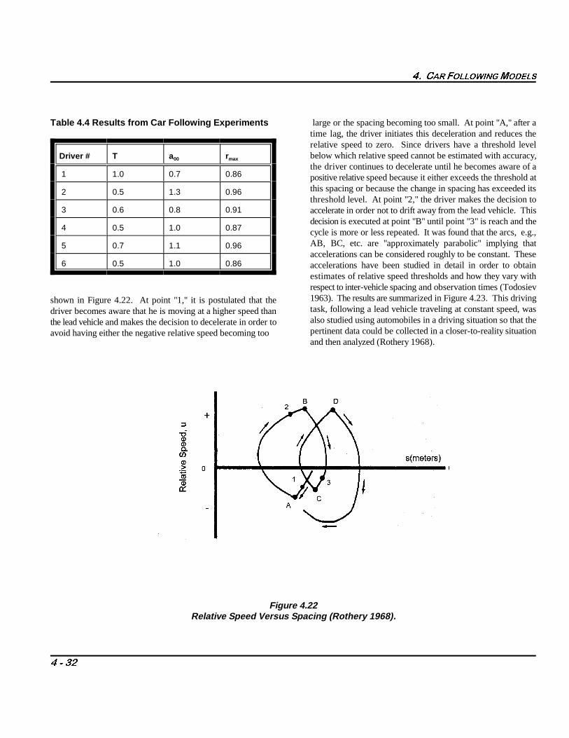
�� &$5 )2//2:,1*02'(/6

� � ��

Table 4.4 Results from Car Following Experiments large or the spacing becoming too small. At point "A," after a

Driver # T a r00 max

1 1.0 0.7 0.86

2 0.5 1.3 0.96

3 0.6 0.8 0.91

4 0.5 1.0 0.87

5 0.7 1.1 0.96

6 0.5 1.0 0.86

shown in Figure 4.22. At point "1," it is postulated that thedriver becomes aware that he is moving at a higher speed thanthe lead vehicle and makes the decision to decelerate in order toavoid having either the negative relative speed becoming too

time lag, the driver initiates this deceleration and reduces therelative speed to zero. Since drivers have a threshold levelbelow which relative speed cannot be estimated with accuracy,the driver continues to decelerate until he becomes aware of apositive relative speed because it either exceeds the threshold atthis spacing or because the change in spacing has exceeded itsthreshold level. At point "2," the driver makes the decision toaccelerate in order not to drift away from the lead vehicle. Thisdecision is executed at point "B" until point "3" is reach and thecycle is more or less repeated. It was found that the arcs, e.g.,AB, BC, etc. are "approximately parabolic" implying thataccelerations can be considered roughly to be constant. Theseaccelerations have been studied in detail in order to obtainestimates of relative speed thresholds and how they vary withrespect to inter-vehicle spacing and observation times (Todosiev1963). The results are summarized in Figure 4.23. This drivingtask, following a lead vehicle traveling at constant speed, wasalso studied using automobiles in a driving situation so that thepertinent data could be collected in a closer-to-reality situationand then analyzed (Rothery 1968).

Figure 4.22Relative Speed Versus Spacing (Rothery 1968).

�xn�1(t�,) �i[ �xn(t) �xn�1(t)]

�� &$5 )2//2:,1*02'(/6

� � ��

(4.64)

Figure 4.23Relative Speed Thresholds Versus Inter-Vehicle Spacing for

Various Values of the Observation Time. (Rothery 1968).

The interesting element in these latter results is that the character speed stimulus is positive or negative. This effect can be takenof the motion as exhibited in Figure 4.22 is much the same. into account by rewriting our basic model as:However, the range of relative speeds at a given spacing thatwere recorded are much lower than those measured on thesimulator. Of course the perceptual worlds in these two tests areconsiderably different. The three dimensional aspects of the testtrack experiment alone might provide sufficient additional cues where � = � or � depending on whether the relative speed isto limit the subject variables in contrast to the two dimensional greater or less than zero.CRT screen presented to the 'driver' in the simulator. In anycase, thresholds estimated in driving appear to be less than those A reexamination of about forty vehicle following tests that weremeasured via simulation. carried out on test tracks and in vehicular tunnels indicates,

Asymmetry Car Following Studies. One car followingexperiment was studied segment by segment using a modelwhere the stimulus included terms proportional to deviationsfrom the mean inter-vehicle spacing, deviations from the meanspeed of the lead vehicle and deviations from the mean speed ofthe following car (Hankin and Rockwell 1967). An interestingresult of the analysis of this model is that it implied anasymmetry in the response depending on whether the relative

i + -

without exception, that such an asymmetry exists (Herman andRothery 1965). The average value of � is �10 percent greater-

than � . The reason for this can partly be attributed to the fact+

that vehicles have considerably different capacities to accelerateand decelerate. Further, the degree of response is likely to bedifferent for the situations where vehicles are separatingcompared to those where the spacing is decreasing. This effectcreates a special difficulty with car following models as isdiscussed in the literature (Newell 1962; Newell 1965). One of

�� &$5 )2//2:,1*02'(/6

� � ��

the principal difficulties is that in a cyclic change in the lead The associated units for these estimates are ft/sec, ft /sec, andvehicle's speed - accelerating up to a higher speed and then miles/car, respectively. As illustrated in this table, excellentreturning to the initial speed, the asymmetry in acceleration and agreement is obtained with the reciprocal spacing model. Howdeceleration of the following car prevents return to the original well these models fit the macroscopic data is shown in Figurespacing. With n such cycles, the spacing continues to increasethereby creating a drifting apart of the vehicles. A relaxationprocess needs to be added to the models that allows for thisasymmetry and also allows for the return to the correct spacing.

4.4.2 Macroscopic Observations: Single Lane Traffic

Several data collections on single lane traffic have been carriedout with the specific purpose of generating a large sample fromwhich accurate estimates of the macroscopic flow characteristicscould be obtained. With such a data base, direct comparisonscan be made with microscopic, car following estimates -particularly when the car following results are obtained on thesame facility as the macroscopic data is collected. One of thesedata collections was carried out in the Holland Tunnel (Edie etal. 1963). The resulting macroscopic flow data for this 24,000vehicle sample is shown in Table 4.5.

The data of Table 4.5 is also shown in graphical form, Figures4.24 and 4.25 where speed versus concentration and flow versusconcentration are shown, respectively. In Figure 4.24, speedversus vehicle concentration for data collected in the HollandTunnel is shown where each data point represents a speed classof vehicles moving with the plotted speed ± 1.61 m/sec. InFigure 4.25, flow versus vehicle concentration is shown; thesolid points are the flow values derived from the speed classesassuming steady-state conditions. (See Table 4.5 and Figure4.24.) Also included in Figure 4.25 are one-minute average flowvalues shown as encircled points. (See Edie et al. 1963). Usingthis macroscopic data set, estimates for three sensitivitycoefficients are estimated for the particular car following modelsthat appear to be of significance. These are: a , a , and a .1,0 2,1 2,0

These are sometimes referred to as the Reciprocal SpacingModel, Edie's Model, and Greenshields' Model, respectively.The numerical values obtained are shown and compared with themicroscopic estimates from car following experiments for thesesame parameters.

2

4.26, where the speed versus vehicle concentration data isgraphed together with the curves corresponding to the steady-state speed-concentration relations for the various indicatedmodels. The data appears in Figure 4.24 and 4.25.

The curves are least square estimates. All three models providea good estimate of the characteristic speed (i.e., the speed atoptimum flow, namely 19, 24, and 23 mi/h for the reciprocalspacing, reciprocal spacing squared, and speed reciprocalspacing squared models, respectively).

Edie's original motivation for suggesting the reciprocal spacingspeed model was to attempt to describe low concentration, non-congested traffic. The key parameter in this model is the "meanfree speed", i.e., the vehicular stream speed as the concentrationgoes to zero. The least squares estimate from the macroscopicdata is 26.85 meters/second.

Edie also compared this model with the macroscopic data in theconcentration range from zero to 56 vehicles/kilometer; thereciprocal spacing model was used for higher concentrations(Edie 1961). Of course, the two model fit is better than any onemodel fitted over the entire range, but marginally (Rothery1968). Even though the improvement is marginal there is anapparent discontinuity in the derivative of the speed-concentration curve. This discontinuity is different than thatwhich had previously been discussed in the literature. It hadbeen suggested that there was an apparent break in the flowconcentration curve near maximum flow where the flow dropssuddenly (Edie and Foote 1958; 1960; 1961). That type ofdiscontinuity suggests that the u-k curve is discontinuous.

However, the data shown in the above figures suggest that thecurve is continuous and its derivative is not. If there is adiscontinuity in the flow concentration relation near optimumflow it is considerably smaller for the Holland Tunnel than hasbeen suggested for the Lincoln Tunnel. Nonetheless, theapparent discontinuity suggests that car following may bebimodal in character.

�� &$5 )2//2:,1*02'(/6

� � ��

Table 4.5 Macroscopic Flow Data

Speed Average Spacing Concentration Number of(m/sec) (m) (veh/km) Vehicles

2.1 12.3 80.1 22

2.7 12.9 76.5 58

3.3 14.6 67.6 98

3.9 15.3 64.3 125

4.5 17.1 57.6 196

5.1 17.8 55.2 293

5.7 18.8 52.6 436

6.3 19.7 50 656

6.9 20.5 48 865

7.5 22.5 43.8 1062

8.1 23.4 42 1267

8.7 25.4 38.8 1328

9.3 26.6 37 1273

9.9 27.7 35.5 1169

10.5 30 32.8 1096

11.1 32.2 30.6 1248

11.7 33.7 29.3 1280

12.3 33.8 26.8 1162

12.9` 43.2 22.8 1087

13.5 43 22.9 1252

14.1 47.4 20.8 1178

14.7 54.5 18.1 1218

15.3 56.2 17.5 1187

15.9 60.5 16.3 1135

16.5 71.5 13.8 837

17.1 75.1 13.1 569

17.7 84.7 11.6 478

18.3 77.3 12.7 291

18.9 88.4 11.1 231

19.5 100.4 9.8 169

20.1 102.7 9.6 55

20.7 120.5 8.1 56

�� &$5 )2//2:,1*02'(/6

� � ��

Note: Each data point represents a speed class of vehicles moving with the plotted speed ± 1 ft/sec (See Table 4.4).

Figure 4.24Speed Versus Vehicle Concentration (Edie et al. 1963).

Note: The solid points are the flow values derived from the speed classes assuming steady-state condition. Also included inFigure 4.25 are one minute average flow values shown as encircled points.

Figure 4.25Flow Versus Vehicle Concentration (Edie et al. 1963).

�� &$5 )2//2:,1*02'(/6

� � ��

Figure 4.26Speed Versus Vehicle Concentration (Rothery 1968).

Table 4.6 flow variables without resorting to using two differentParameter Comparison(Holland Tunnel Data)

Parameters Estimates EstimatesMicroscopic Macroscopic

a 26.8 27.81,0

a 0.57 0.122, 0

a (123) (54)2,1-1 -1

A totally different approach to modeling traffic flow variableswhich incorporates such discontinuities can be found in theliterature. Navin (1986) and Hall (1987) have suggested thatcatastrophe theory (Thom 1975; Zeeman 1977) can be used asa vehicle for representing traffic relationships. Specifically,Navin followed the two regime approach proposed by Edie andcited above and first suggested that traffic relations can berepresented using the cusp catastrophe. A serious attempt toapply such an approach to actual traffic data in order to represent

expressions or two different sets of parameters to one expressionhas been made by Hall (1987). More recently, Acha-Daza andHall (1994) have reported an analysis of freeway data usingcatastrophe theory which indicates that such an approach caneffectively be applied to traffic flow. Macroscopic data has alsobeen reported on single lane bus flow. Here platoons of tenbuses were studied (Rothery et al. 1964).

Platoons of buses were used to quantify the steady-state streamproperties and stability characteristics of single lane bus flow. Ideally, long chains of buses should be used in order to obtainthe bulk properties of the traffic stream and minimize the endeffects or eliminate this boundary effect by having the leadvehicle follow the last positioned vehicle in the platoon using acircular roadway. These latter type of experiments have beencarried out at the Road Research Laboratory in England(Wardrop 1965; Franklin 1967).

In the platoon experiments, flow rates, vehicle concentration,and speed data were obtained. The average values for the speedand concentration data for the ten bus platoon are shown inFigure 4.28 together with the numerical value for the parameter

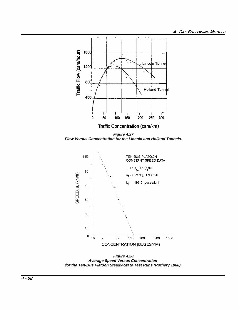
�� &$5 )2//2:,1*02'(/6

� � ��

Figure 4.27Flow Versus Concentration for the Lincoln and Holland Tunnels.

Figure 4.28Average Speed Versus Concentration

for the Ten-Bus Platoon Steady-State Test Runs (Rothery 1968).

�� &$5 )2//2:,1*02'(/6

� � ��

a = 53 km/h which is to be compared to that obtained from the1,0

two bus following experiments discussed earlier namely, 58km/h. Given these results, it is estimated that a single lane ofstandard size city buses is stable and has the capacity of over65,000 seated passengers/hour. An independent check of thisresult has been reported (Hodgkins 1963). Headway times and

speed of clusters of three or more buses on seven differenthighways distributed across the United States were measuredand concluded that a maximum flow for buses would beapproximately 1300 buses/hour and that this would occur atabout 56 km/h.

4.5 Automated Car Following

All of the discussion in this chapter has been focused on manual Mechanical Laboratory (Oshima et al. 1965), the Transportationcar following, on what drivers do in following one or more other Road Research Laboratory (Giles and Martin 1961; Cardewvehicles on a single lane of roadway. Paralleling these studies, 1970), Ford Motor Corporation (Cro and Parker 1970) and theresearch has also focused on developing controllers that would Japanese Automobile Research Institute (Ito 1973). During theautomatically mimic this task with specific target objectives in past several decades three principal research studies in this arenamind. stand out: a systems study of automated highway systems

At the 1939 World's Fair, General Motors presented program on numerous aspects of automated highways conductedconceptually such a vision of automated highways where at The Ohio State University from 1964-1980, and the Programvehicles were controlled both longitudinally (car following) and on Advanced Technology for the Highway (PATH) at thelaterally thereby freeing drivers to take on more leisurely University of California, Berkeley from about 1976 to theactivities as they moved at freeway speeds to their destinations. present. Three overviews and detailed references to milestonesIn the intervening years considerable effort has been extended of these programs can be found in the literature: Bender (1990),towards the realization of this transportation concept. One prime Fenton and Mayhan (1990), and Shladover et al. (1990),motivation for such systems is that they are envisioned to provide respectively.more efficient utilization of facilities by increasing roadwaycapacity particularly in areas where constructing additional The car following elements in these studies are focused onroadway lanes is undesirable and or impractical, and in addition, developing controllers that would replace driver behavior, carrymight improve safety levels. The concept of automated out the car following task and would satisfy one or morehighways is one where vehicles would operate on both performance and/or safety criteria. Since these studies haveconventional roads under manual control and on specially essentially been theoretical, they have by necessity required theinstrumented guideways under automatic control. Here we are difficult task of modeling vehicle dynamics. Given a controllerinterested in automatic control of the car following task. Early for the driver element and a realistic model representation ofresearch in this arena was conducted on both a theoretical and vehicle dynamics a host of design strategies and issues have beenexperimental basis and evaluated at General Motors Corporation addressed regarding inter-vehicular spacing control, platoon(Gardels 1960; Morrison 1961; Flory et al. 1962), Ohio State configurations, communication schemes, measurement andUniversity (Fenton 1968; Bender and Fenton 1969; Benton timing requirements, protocols, etc. Experimental verificationset al. 1971; Bender and Fenton 1970), Japan Governmental of these elements are underway at the present time by PATH.

conducted at General Motors from 1971-1981, a long-range

�� &$5 )2//2:,1*02'(/6

� � ��

4.6 Summary and Conclusions

Historically, the subject of car following has evolved over the this chapter has addressed in order. First, it provides apast forty years from conceptual ideas to mathematical model mathematical model of a relative common driving task anddescriptions, analysis, model refinements resulting from provides a scientific foundation for understanding this aspect ofempirical testing and evaluation and finally extensions into the driving task; it provides a means for analysis of local andadvanced automatic vehicular control systems. These asymptotic stability in a line of vehicles which carry implicationsdevelopments have been overlapping and interactive. There with regard to safety and traffic disruptions and other dynamicalhave been ebbs and flows in both the degree of activity and characteristics of vehicular traffic flow; it provides a steady stateprogress made by numerous researchers that have been involved description of single lane traffic flow with associated roadin the contributions made to date. capacity estimates; it provides a stepping stone for extension into

The overall importance of the development of the subject of car will undoubtedly continue to provide stimulus andfollowing can be viewed from five vantage points, four of which encouragement to scientists working in related areas of traffic

advance automatic vehicle control systems; and finally, it has and

theory.

References

Acha-Daza, J. A. and F. L. Hall (1994). Application ofCatastrophe Theory to Traffic Flow Variables.Transportation Research - B, 28B(3). Elsevier ScienceLtd., pp. 235-250. Constantine, T. and A. P. Young (1967). Traffic Dynamics:

Babarik, P. (1968). Automobile Accidents and Driver Car Following Studies. Traffic Engineering and Control 8,Reaction Pattern. Journal of Applied Psychology, 52(1),pp. 49-54. Cumming, R. W. (1963). The Analysis of Skills in Driving.

Barbosa, L. (1961). Studies on Traffic Flow Models. ReportsNo. 202A-1. The Ohio State University Antenna Darroch, J. N. and R. W. Rothery (1973). Car Following andLaboratory.

Bender, J. G. (1971). An Experimental Study of Vehicle Symposium on the Theory of Traffic Flow andAutomatic Longitudinal Control. IEEE Transactions onVehicular Technology, VT-20, pp. 114-123.

Bender, J. G. (1991). An Overview of Systems Studies ofAutomated Highway Systems. IEEE Transactions onVehicular Technology 40(1). IEEE Vehicular TechnologySociety, pp. 82-99. Drew, D. R. (1965). Deterministic Aspects of Freeway

Bender, J. G. and R. E. Fenton (1969). A Study of Automatic Operations and Control. Highway Research Record, 99,Car Following. IEEE Transactions on VehicularTechnology, VT-18, pp. 134-140. Edie, L. C. (1961). Car-Following and Steady State Theory

Cardew, K. H. F. (1970). The Automatic Steering of Vehicles for Non-Congested Traffic. Operations Research 9(1),-An Experimental System Fitted to a Citroen Car. RL 340, Road Research Laboratories. Edie, L. C. and E. Baverez (1967). Generation and

Chandler, F. E., R. Herman, and E. W. Montroll, (1958). Traffic Dynamics: Studies in Car Following, Operations Science Proceedings of the 3rd International Symposium onResearch, 6, pp. 165-184. the Theory of Traffic Flow. L.C. Edie, R. Herman and R.W.

Chow, T. S. (1958). Operational Analysis of a TrafficDynamics Problem. Operations Research, 6(6),pp. 165-184.

pp. 551.

Journal of the Australian Road Research Board 1, pp. 4.

Spectral Analysis. Proceedings of the 5th International

Transportation. Ed. Newell, G. F., American ElsevierPublishing Co., New York.

Drake, J. S., J. L. Schofer, and A. D. May, Jr. (1967). AStatistical Analysis of Speed Density Hypotheses. HighwayResearch Record 154, pp. 53-87.

pp. 48-58.

pp. 66-76.

Propagation of Stop-Start Waves. Vehicular Traffic

Rothery (Eds.). American Elsevier, New York.

�� &$5 )2//2:,1*02'(/6

� � ��

Edie, L. C. and R. S. Foote, (1958). Traffic Flow in Tunnels. Greenburg, H. (1959). An Analysis of Traffic Flow.Proceedings of the Highway Research Board, 37, Operations Research 7(I), pp. 255-275.pp. 334-344.

Edie, L. C. and R. S. Foote (1960). Effect of Shock Waves on Proceedings of the Highway Research Board, 14, 468.Tunnel Traffic Flow. Proceedings of the Highway Research Hall, F. L. (1987). An Interpretation of Speed-FlowBoard, 39, pp. 492-505.

Edie, L. C., and R. S. Foote (1961). Experiments on Single Transportation Research, 21A, pp. 335-344.Lane Flow in Tunnels. Theory of Traffic Flow Proceedings Hankin, A. and T. H. Rockwell (1967). A Model of Carof the Theory of Traffic Flow. Ed. R. Herman. ElsevierPub. Co., Amsterdam, pp. 175-192.

Edie, L. C., R. S. Foote, R. Herman, and R. W. Rothery(1963). Analysis of Single Lane Traffic Flow. TrafficEngineering, 21, 27.

Ellson, D. G. (1949). The Application of Operational Analysisto Human Motor Behavior. Psychology Review 9,pp. 56.

Fenton, R. E. (1968). One Approach to Highway Automation.Proceedings IEEE 56; pp. 556-566.

Fenton, R. E. and R. J. Mayhan (1991). Automated HighwayStudies at The Ohio State University - An Overview. IEEETransaction on Vehicular Technology 40(1); IEEEVehicular Technology Society, pp. 100-113.

Flory, L. E. (1962). Electronic Techniques in a System ofHighway Vehicle Control. RCA Review 23, pp. 293-310.

Forbes, T. W., M. J. Zagorski, E. L. Holshouser, and W. A.Deterline (1959). Measurement of Driver Reaction toTunnel Conditions. Proceedings of the Highway ResearchBoard 37, pp. 345-357.

Gardels, K. (1960). Automatic Car Controls for ElectronicHighways. GM Research Laboratories Report GMR-276,Warren, MI.

Gazis, D. C., R. Herman, and R. B. Potts (1959). CarFollowing Theory of Steady State Traffic Flow. OperationsResearch 7(4), pp. 499-505.

Gazis, D. C., R. Herman, and R. W. Rothery (1961). Non-Linear Follow the Leader Models of Traffic Flow.Operations Research, 9, pp. 545-567.

Gazis, D. C., R. Herman, and R. W. Rothery (1963). Analytical Methods in Transportation: Mathematical Car-Following Bonn, Germany.Theory of Traffic Flow. Journal of the EngineeringMechanics Division, ASCE Proc. Paper 3724 89(Paper372), pp. 29-46. Hodgkins, E. A. (1963). Effect of Buses on Freeway Capacity.

Giles, C. G. and J. A. Martin (1961). Cable Installation forVehicle Guidance Investigation in the New Research Trackat Crowthorne. Rep RN/4057/CGG, Road ResearchLaboratory, Crowthorne, England.

Greenshields, B. D. (1935). A Study of Traffic Capacity.

Concentration Relationships Using Catastrophe Theory.

Following Derived Empirically by Piece-Wise RegressionAnalysis. Vehicular Traffic Science Proceedings of the 3rdInternational Symposium on the Theory of Traffic Flow.L.C. Edie, R. Herman and R.W. Rothery (Eds.). AmericanElsevier, New York.

Harris, A. J. (1964). Following Distances, Braking Capacityand the Probability of Danger of Collision BetweenVehicles. Australian Road Research Board, Proceedings 2,Part 1, pp. 496-412.

Helly, W. (1959). Dynamics of Single-Lane Vehicular TrafficFlow. Research Report No. 2, Center for OperationsResearch, MIT. Cambridge, Mass.

Herman, R., E. W. Montroll, R. B. Potts and R. W. Rothery(1958). Traffic Dynamics: Analysis of Stability in CarFollowing. Operations Research, E. 17, pp. 86-106.

Herman, R. and R. B. Potts (1959). Single Lane TrafficTheory and Experiment. Proceedings Symposium onTheory of Traffic Flow. Ed. R. Herman, ElsevierPublications Co., pp. 120-146.

Herman, R. and R. W. Rothery (1962). Microscopic andMacroscopic Aspects of Single Lane Traffic Flow.Operations Research, Japan, pp. 74.

Herman, R. and R. W. Rothery (1965). Car Following andSteady-State Flow. Proceedings of the 2nd InternationalSymposium on the Theory of Traffic Flow. Ed J. Almond,O.E.C.D., Paris.

Herman, R. and R. W. Rothery (1969). Frequency andAmplitude Dependence of Disturbances in a TrafficStream. Proceedings of 4th International Symposium on theTheory of Traffic Flow, Ed. W. Leutzbach and P. Baron.

Highway Capacity Manual (1950). U.S. Government PrintingOffice, Washington, DC.

Presentation at the 43rd Annual Meeting of the HighwayResearch Board 33. Highway Research Abstracts, pp. 69.

Ito, T. (1973). An Automatic Drivers System of Automobilesby Guidance Cables. Society of Automotive Engineering(730127).

�� &$5 )2//2:,1*02'(/6

� � ��

Kometani, E. and T. Suzaki (1958). On the Stability of TrafficFlow. J. Operations Research, Japan 2, pp. 11-26.

Lam, T. and R. W. Rothery (1970). Spectral Analysis ofSpeed fluctuations on a Freeway. Transportation Science4(3).

Lee, G. (1966). A Generalization of Linear Car-FollowingTheory. Operations Research 14(4), pp. 595-606.

May, A. D. and H.E.M. Keller (1967). Non-Integer CarFollowing Models. Highway Research Record 199, pp. 19-32.

Michaels, R. M. (1963). Perceptual Factors in CarFollowing. Proceedings of the 2nd InternationalSymposium on the Theory of Road Traffic Flow (London,England), OECD.

Navin, F. P. D. (1986). Traffic Congestion Catastrophes. Transportation Planning and Technology 11, pp. 19-25.

Newell, G. F. (1961). Nonlinear Effects in the Dynamics ofCar Following. Operations Research 9(2), pp. 209-229.

Newell, G. F. (1962). Theories of Instability in DenseHighway Traffic. J. Operations Research Society of Japan5(1), pp. 9-54.

Oshima, R. (1965). Control System for Automobile Driving. Proceedings of the Tokyo 1FAC Symposium, pp. 347-357.Pipes, L. A. (1951). A Proposed Dynamic Analogy of Traffic.

ITTE Report, Institute of Transportation and TrafficEngineering, University of California, Berkeley.

Pipes, L. A. (1953). An Operational Analysis of TrafficDynamics. Journal of Applied Physics 24, pp. 271-281.

Reuschel, A. (1950). Fahrzeugbewegungen in der KolonneBeigleichformig beschleunigtem oder vertzogertenLeitfahrzeub, Zeit. D. Oster. Ing. U. Architekt Vereines Ed.(Vehicle Movements in a Platoon with UniformAcceleration or Deceleration of the Lead Vehicle), pp. 50-62 and 73-77.

Rothery, R. W., R. Silver, R. Herman and C. Torner (1964). Analysis of Experiments on Single Lane Bus Flow.Operations Research 12, pp. 913.

Shladover, S. E., C. A. Desoer, J. D. Hedrick, M. Tomizuka,J. Walrand, W. B. Zhang, D. H. McMahon, H. Peng, S. Shiekholeslam, and N. McKeown (1991). AutomatedVehicle Control Developments in the PATH Program.IEEE Transactions on Vehicular Technology 40(1), pp. 114-130.

Taylor, F. V. (1949). Certain Characteristics of the HumanServe. Electrical Engineering 68, pp. 235.

Telfor, G. W. (1931). The Refractory Phase of Voluntary andAssociative Responses. Journal of ExperimentalPsychology, 14, pp. 1.

Thorn, R. (1975). Structural Stability and Morphogenesis. An English Translation by D.H. Fowler. John Wiley &Sons, New York.

Todosiev, E. P. (1963). The Action Point Model of the DriverVehicle System. Report No. 202A-3. Ohio StateUniversity, Engineering Experiment Station, Columbus,Ohio.

Tuck, E. (1961). Stability of Following in Two Dimensions. Operations Research, 9(4), pp. 479-495.

Tustin, A. (1947). The Nature of the Operator Response inManual Control and its Implication for Controller Design.J.I.E.E. 92, pp. 56.

Unwin, E. A. and L. Duckstein (1967). Stability of Reciprocal-Spacing Type Car Following Models.Transportation Science, 1, pp. 95-108.

Uttley, A. (1941). The Human Operator as an IntermittentServo. Report of the 5th Meeting of Manual TrackingPanel, GF/171.SR1A.

Wardrop, J. G. (1965). Experimental Speed/Flow Relations ina Single Lane. Proceedings of the 2nd InternationalSymposium on the Theory of Road Traffic Flow. Ed. J.Almond O.E.C.D.

Zeeman, E. C. (1977). Catastrophe Theory. Selected Papers1972-1977. Addison-Wesley, London.