capital budgeting risk analysis 1finance - pedro barroso

Capital BudgetingRisk Analysis

1Finance - Pedro Barroso

Sensitivity, Scenario, and Break-Even

• Allows us to look behind the NPV number to see how stable our estimates are

• When working with spreadsheets, try to build your model so that you can adjust variables in a single cell and have the NPV calculations update accordingly


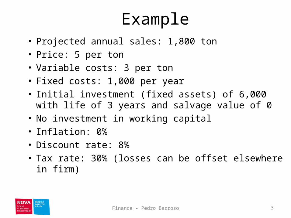
Example• Projected annual sales: 1,800 ton• Price: 5 per ton• Variable costs: 3 per ton• Fixed costs: 1,000 per year• Initial investment (fixed assets) of 6,000 with life of 3

years and salvage value of 0• No investment in working capital• Inflation: 0%• Discount rate: 8%• Tax rate: 30% (losses can be offset elsewhere in firm)


Example

Microsoft Office Excel 97-2003 Worksheet

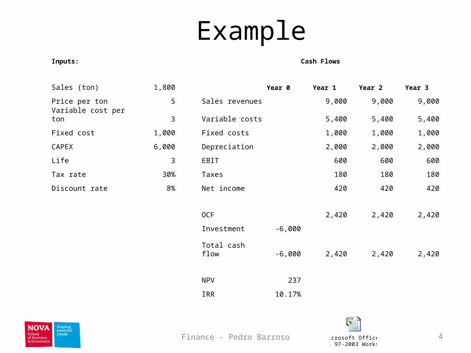
Inputs: Cash Flows

Sales (ton) 1,800 Year 0 Year 1 Year 2 Year 3

Price per ton 5 Sales revenues 9,000 9,000 9,000

Variable cost per ton 3 Variable costs 5,400 5,400 5,400

Fixed cost 1,000 Fixed costs 1,000 1,000 1,000

CAPEX 6,000 Depreciation 2,000 2,000 2,000

Life 3 EBIT 600 600 600

Tax rate 30% Taxes 180 180 180

Discount rate 8% Net income 420 420 420

OCF 2,420 2,420 2,420

Investment -6,000

Total cash flow -6,000 2,420 2,420 2,420

NPV 237

IRR 10.17%


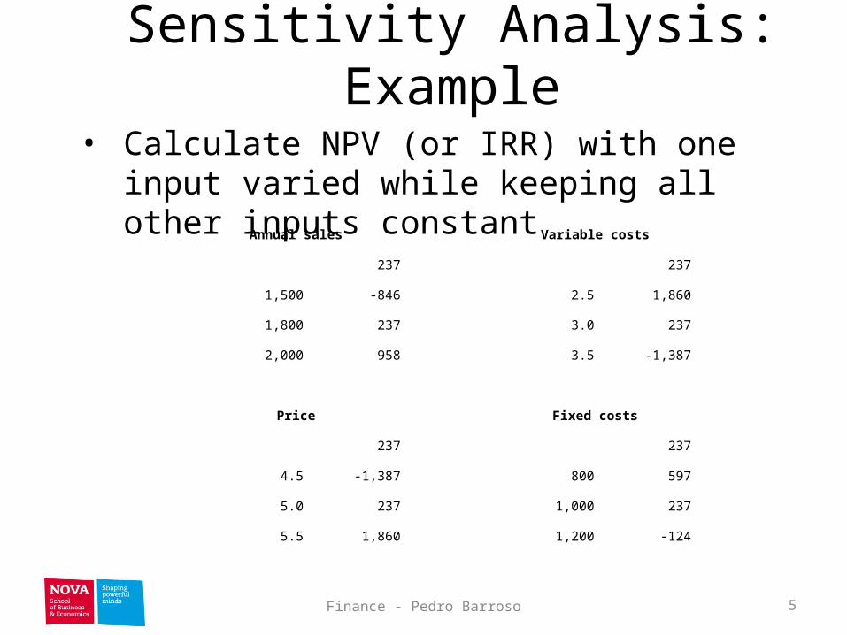
Sensitivity Analysis: Example• Calculate NPV (or IRR) with one input varied while

keeping all other inputs constantAnnual sales Variable costs

237 237

1,500 -846 2.5 1,860

1,800 237 3.0 237

2,000 958 3.5 -1,387

Price Fixed costs

237 237

4.5 -1,387 800 597

5.0 237 1,000 237

5.5 1,860 1,200 -124


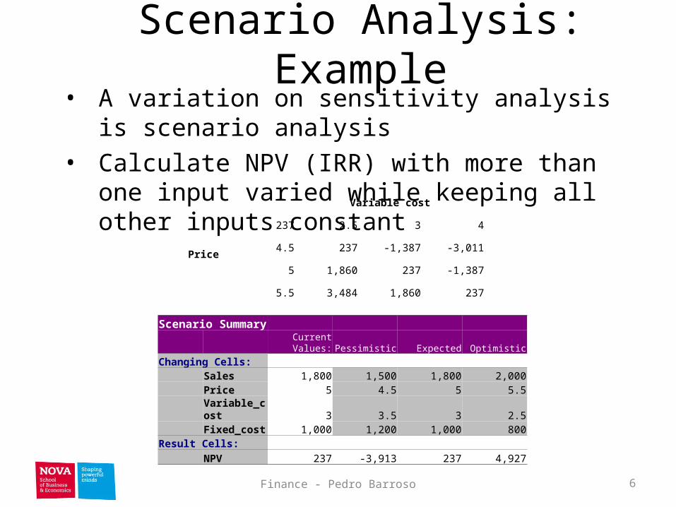
Scenario Analysis: Example• A variation on sensitivity analysis is scenario analysis• Calculate NPV (IRR) with more than one input varied

while keeping all other inputs constantVariable cost

Price

237 2.5 3 4

4.5 237 -1,387 -3,011

5 1,860 237 -1,387

5.5 3,484 1,860 237

Scenario Summary

Current Values: Pessimistic Expected OptimisticChanging Cells: Sales 1,800 1,500 1,800 2,000 Price 5 4.5 5 5.5 Variable_cost 3 3.5 3 2.5 Fixed_cost 1,000 1,200 1,000 800Result Cells: NPV 237 -3,913 237 4,927


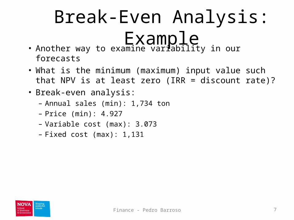
Break-Even Analysis: Example• Another way to examine variability in our forecasts• What is the minimum (maximum) input value such that NPV is

at least zero (IRR = discount rate)?• Break-even analysis:

– Annual sales (min): 1,734 ton– Price (min): 4.927– Variable cost (max): 3.073– Fixed cost (max): 1,131


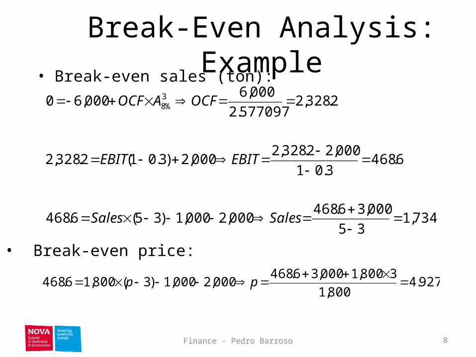
Break-Even Analysis: Example• Break-even sales (ton):

734,135

000,36.468000,2000,1)35(6.468

6.4683.01

000,22.328,2000,2)3.01(2.328,2

2.328,2577097.2

000,6000,60 3

%8

SalesSales

EBITEBIT

OCFAOCF

• Break-even price:

927.4800,1

3800,1000,36.468000,2000,1)3(800,16.468

pp


Real Options

• One of the fundamental insights of modern finance theory is that options have value

• Because corporations make decisions in a dynamic environment, they have options that should be considered in project valuation

• Traditional NPV does not include options value (always zero or positive)


Real Options• Option to Expand– Has value if demand turns out to be higher than

expected

• Option to Abandon– Has value if demand turns out to be lower than

expected

• Option to Delay– Has value if the underlying variables are changing

with a favorable trend


Discounted CF and Options• We can calculate the market value of a project as the sum of the

NPV of the project without options and the value of the managerial options implicit in the project:

NPV + Options

Example: Comparing a specialized machine versus a more versatile machine; if they both cost about the same and last the same amount of time, more versatile machine is more valuable because it comes with options


Option to Abandon: Example• Suppose we are drilling an oil well. The drilling rig

costs $300 today, and in one year the well is either a success or a failure

• Outcomes are equally likely. Discount rate is 10%

• PV of the successful payoff at time one is $575

• PV of the unsuccessful payoff at time one is $0


Option to Abandon: Example

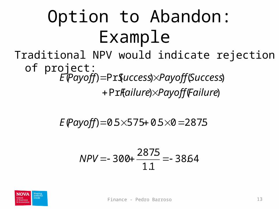
Traditional NPV would indicate rejection of project:

64.381.1

5.287300

5.28705.05755.0)(

)()Pr()()Pr()(

NPV

PayoffE

FailurePayoffFailureSuccessPayoffSuccessPayoffE



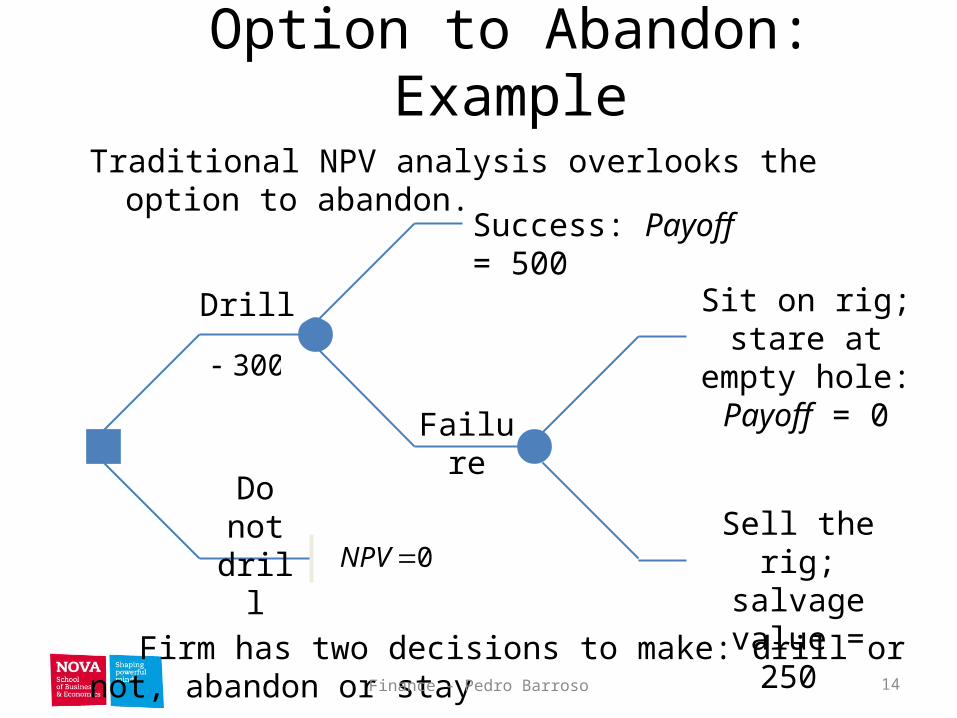
Firm has two decisions to make: drill or not, abandon or stay

Do not drill

Drill

0NPV

Failure

Success: Payoff = 500

Sell the rig; salvage value

= 250

Sit on rig; stare at empty hole:

Payoff = 0

Traditional NPV analysis overlooks the option to abandon.

300



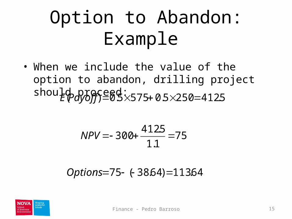
• When we include the value of the option to abandon, drilling project should proceed:

64.113)64.38(75

751.1

5.412300

5.4122505.05755.0)(

Options

NPV

PayoffE


Option to Delay: Example

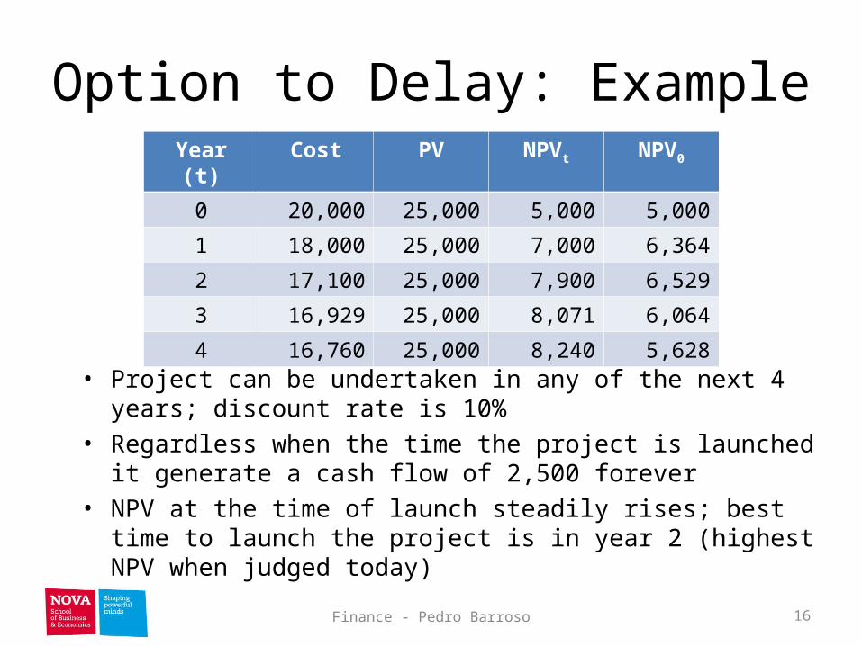
• Project can be undertaken in any of the next 4 years; discount rate is 10%

• Regardless when the time the project is launched it generate a cash flow of 2,500 forever

• NPV at the time of launch steadily rises; best time to launch the project is in year 2 (highest NPV when judged today)

Year (t) Cost PV NPVt NPV0

0 20,000 25,000 5,000 5,000

1 18,000 25,000 7,000 6,364

2 17,100 25,000 7,900 6,529

3 16,929 25,000 8,071 6,064

4 16,760 25,000 8,240 5,628


Decision Trees

• Allow us to graphically represent the alternatives available to us in each period and the likely consequences of our actions

• This graphical representation helps to identify the best course of action


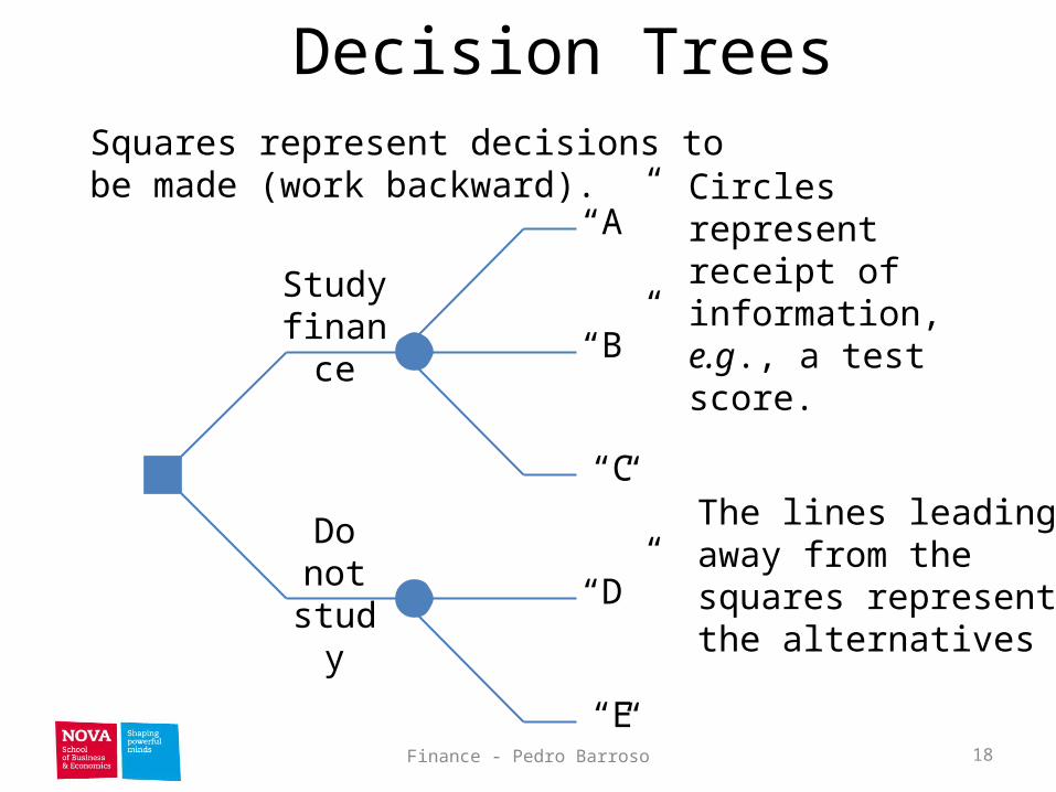
Decision Trees

Do not study

Study finance

Squares represent decisions to be made (work backward). Circles represent

receipt of information, e.g., a test score.

The lines leading away from the squares represent the alternatives

“C”

“A”

“B”

“E”

“D”


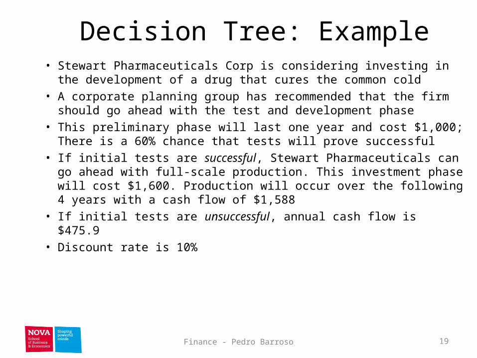
Decision Tree: Example• Stewart Pharmaceuticals Corp is considering investing in the

development of a drug that cures the common cold• A corporate planning group has recommended that the firm

should go ahead with the test and development phase• This preliminary phase will last one year and cost $1,000; There

is a 60% chance that tests will prove successful• If initial tests are successful, Stewart Pharmaceuticals can go

ahead with full-scale production. This investment phase will cost $1,600. Production will occur over the following 4 years with a cash flow of $1,588

• If initial tests are unsuccessful, annual cash flow is $475.9• Discount rate is 10%


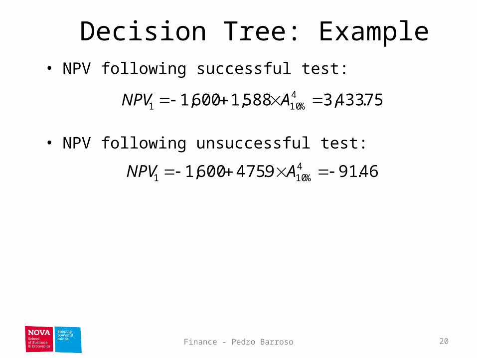
Decision Tree: Example• NPV following successful test:

• NPV following unsuccessful test:

75.433,3588,1600,1 4%101 ANPV

46.919.475600,1 4%101 ANPV


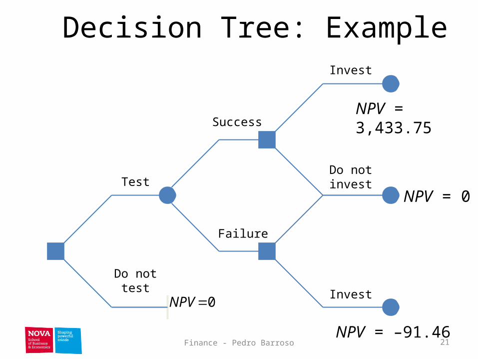
Decision Tree: Example

Do not test

Test

Failure

Success

Do not invest

Invest

Invest0NPV

NPV = 3,433.75

NPV = 0

NPV = –91.4621Finance - Pedro Barroso

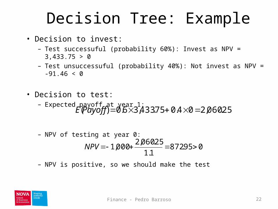
Decision Tree: Example• Decision to invest:

– Test successuful (probability 60%): Invest as NPV = 3,433.75 > 0– Test unsuccessuful (probability 40%): Not invest as NPV = -91.46 < 0

• Decision to test:– Expected payoff at year 1:

– NPV of testing at year 0:

– NPV is positive, so we should make the test

25.060,204.075.433,36.0)( PayoffE

095.8721.1

25.060,2000,1 NPV


capital budgeting risk analysis 1finance - pedro barroso

Documents

finance pedro barroso

options value

npv options example

breakeven analysis

scenario analysis

sensitivity analysis

example breakeven sales

breakeven price