CANoe Product Information

CANoe

2

Table of Contents

1 Introduction to CANoe ............................................................................................................................................................. 5 1.1 Bus Systems and Protocols ...................................................................................................................................................... 6 1.2 Product Concept and Variants ................................................................................................................................................ 6 1.3 Product Components ................................................................................................................................................................ 6 1.4 System Requirements ............................................................................................................................................................... 7 1.5 Additional Usage Scenarios ..................................................................................................................................................... 7 1.5.1 CANoe under „EULA“................................................................................................................................................................ 7 1.5.2 CANoe under “ELA” .................................................................................................................................................................. 7 1.6 Further Information .................................................................................................................................................................. 7

2 Functions.................................................................................................................................................................................... 8 2.1 Special Functions ...................................................................................................................................................................... 9 2.2 Database Support ................................................................................................................................................................... 10

3 Analysis .................................................................................................................................................................................... 10 3.1 Measurement Setup................................................................................................................................................................ 11 3.2 Trace Window .......................................................................................................................................................................... 12 3.3 Graphics Window .................................................................................................................................................................... 13 3.4 Scope Window ......................................................................................................................................................................... 14 3.5 Data Window........................................................................................................................................................................... 15 3.6 Statistics Window .................................................................................................................................................................. 15 3.7 State Tracker ........................................................................................................................................................................... 16 3.8 Write Window ......................................................................................................................................................................... 17 3.9 Video Window.......................................................................................................................................................................... 18 3.10 GPS Window ............................................................................................................................................................................ 19 3.11 Triggers and Filters ................................................................................................................................................................. 19 3.12 Logging/Replay ....................................................................................................................................................................... 20

4 Stimulation/Simulation .......................................................................................................................................................... 20 4.1 Variables and Generators ...................................................................................................................................................... 20 4.1.1 Interactive Generator ............................................................................................................................................................. 20 4.1.2 Signal Generator ..................................................................................................................................................................... 21 4.2 Set Start Values ...................................................................................................................................................................... 22 4.3 Symbol Mapping ...................................................................................................................................................................... 23 4.4 Interaction Layer, Network Management, Transport Protocols ........................................................................................ 23 4.4.1 OEM-Specific Extensions ....................................................................................................................................................... 23 4.4.2 Configuration of the Interaction Layer ................................................................................................................................. 24 4.5 MATLAB/Simulink ................................................................................................................................................................... 24 4.5.1 Further Functions of the CANoe MATLAB/Simulink Integration ....................................................................................... 25 4.5.2 Further Information ................................................................................................................................................................ 26

5 Test ........................................................................................................................................................................................... 26 5.1 Testing ECUs and Networks .................................................................................................................................................. 26 5.2 CANoe RT/VN8900 and CAPL-on-Board .............................................................................................................................. 30 5.3 Vector Tool Platform .............................................................................................................................................................. 30 5.4 CAN/CAN FD Disturbances ................................................................................................................................................... 30 5.5 Further Information ................................................................................................................................................................ 31

CANoe

3

6 Diagnostics .............................................................................................................................................................................. 32 6.1 Further Information ................................................................................................................................................................ 35

7 SoA and AUTOSAR Adaptive ................................................................................................................................................. 36 7.1 Communication Concepts – Current Developement ........................................................................................................... 36 7.2 The CANoe Communication Model ........................................................................................................................................ 36

8 Programming ........................................................................................................................................................................... 37 8.1 CAPL Interface ........................................................................................................................................................................ 37 8.1.1 C-Like Syntax .......................................................................................................................................................................... 37 8.1.2 Event-oriented Control........................................................................................................................................................... 38 8.1.3 Symbolic Access ...................................................................................................................................................................... 38 8.1.4 Application-Specific Language Extensions .......................................................................................................................... 38 8.2 CAPL Browser ......................................................................................................................................................................... 40 8.3 .NET Programming .................................................................................................................................................................. 41 8.4 Debugging ................................................................................................................................................................................ 42 8.4.1 Further Information ................................................................................................................................................................ 42 8.5 Visual Sequencer ..................................................................................................................................................................... 43

9 Panels ....................................................................................................................................................................................... 43

10 Hardware Interfaces ............................................................................................................................................................... 44

11 Interfaces to Other Applications ........................................................................................................................................... 44 11.1 COM Interface ......................................................................................................................................................................... 44 11.1.1 Further Information ................................................................................................................................................................ 45 11.2 FDX ........................................................................................................................................................................................... 45 11.3 ASAM XIL API .......................................................................................................................................................................... 45 11.4 FMI ............................................................................................................................................................................................ 45

12 Option .Scope .......................................................................................................................................................................... 45 12.1 Application Areas .................................................................................................................................................................... 45 12.2 Overview of Advantages ........................................................................................................................................................ 46 12.3 Supported Protocols ............................................................................................................................................................... 46 12.4 Supported Oscilloscope Hardware ........................................................................................................................................ 47 12.5 Oscilloscope Software ............................................................................................................................................................ 47 12.5.1 Configuration Functions ......................................................................................................................................................... 47 12.5.2 Trigger Functions .................................................................................................................................................................... 47 12.5.3 Analysis Functions .................................................................................................................................................................. 48 12.5.4 Offline Functions ..................................................................................................................................................................... 48

13 Option .Sensor ......................................................................................................................................................................... 48 13.1 Application Areas .................................................................................................................................................................... 49 13.2 Supported Sensor Protocols .................................................................................................................................................. 49 13.3 Supported Serial Protocols .................................................................................................................................................... 49 13.4 Highlights ................................................................................................................................................................................. 50

14 Option .SmartCharging .......................................................................................................................................................... 50

15 Option .AMD/XCP ................................................................................................................................................................... 51 15.1 Application Areas .................................................................................................................................................................... 51 15.1.1 Calibration Protocol (XCP) / CAN Calibration Protocol (CCP) ......................................................................................... 51 15.1.2 AUTOSAR Monitoring and Debugging (AMD) ...................................................................................................................... 51 15.2 ECU Access .............................................................................................................................................................................. 52

CANoe

4

15.2.1 Supported Bus Systems and Protocols ................................................................................................................................. 52 15.2.2 VX1000 Measurement and Calibration Interface ................................................................................................................ 52 15.2.3 CSM Measurement Module .................................................................................................................................................... 52 15.2.4 Hardware Debugger Support ................................................................................................................................................. 52 15.3 Overview of Advantages ........................................................................................................................................................ 53 15.4 Functions.................................................................................................................................................................................. 53 15.5 Integration in CANoe .............................................................................................................................................................. 54 15.6 Configuration .......................................................................................................................................................................... 54

16 Functional Extensions for Special Applications ................................................................................................................... 55 16.1 DiVa (Diagnostic Integration and Validation Assistant) .................................................................................................... 55

17 Training .................................................................................................................................................................................... 55

V6.1 11/2018

Valid for CANoe from version 11.0 SP3.

This document presents the CANoe use areas of analysis, stimulation/simulation, testing, diagnostics and their individual functions. The document also contains a brief overview of programming in CANoe, supplemental options and programs as well as hardware and software interfaces.

Product information and technical data on CANoe with the .FlexRay, .LIN and .MOST options are presented in separate documents.

CANoe

5

1 Introduction to CANoe

CANoe is a versatile tool for the development, testing and analysis of entire ECU networks as well as individual ECUs. It supports network designers, development and test engineers at OEMs and suppliers over the entire development process – from planning to the start-up of entire distributed systems or individual ECUs.

At the beginning of the development process, CANoe is used to create simulation models which simulate the behavior of the ECUs. Over the further course of ECU development, these models serve as the basis for analysis, testing and the integration of bus systems and ECUs. This makes it possible to detect problems early and correct them. Graphic and text based analysis windows are provided for evaluating the results.

CANoe contains the Test Feature Set for easy and automated test execution. It is used to model and execute sequential test sequences and automatically generate a test report. The Diagnostic Feature Set is also available within CANoe for diagnostic communications with the ECU.

Figure 1: CANoe user interface

CANoe

6

1.1 Bus Systems and Protocols

In CANoe, various options are available for the different bus systems and CAN-based protocols, and any combination of these options may be used.

CANoe supports the following bus systems: CAN, CAN FD, LIN, MOST, FlexRay, J1708, Ethernet, K-Line, A429, WLAN and AFDX®1

Option .CAN is the basis for these supported CAN-based protocols: J1939, ISO 11783, CANopen, GMLAN, CANaero. Others upon request.

You will find detailed information on the options in separate product information documents.

1.2 Product Concept and Variants

CANoe is available in the following variants for special purposes at OEMs and suppliers:

> With full range of functionality

> As a Runtime (run) variant with unmodifiable simulations, full range of analysis functions and easy activation/deactivation of individual network nodes. This variant is intended for users who wish to quickly and simply test their ECU in interaction with a prescribed remaining bus simulation.

> As a Project Execution (pex) variant with just a graphic user interface. The test cases and results are very easy to control without requiring special evaluation of the underlying messages.

The CANoe/CANalyzer compatibility mode lets you use both programs, e.g. within a project or an organization, by exchanging uniform configurations. Then the appropriate program can be used in the optimal variant for each use case. During ECU development, the full variant of CANoe is used, while system integrators and test drivers can use the same configuration in CANalyzer to test the bus communications.

1.3 Product Components

The product contents depend on the selected product variant. The full version contains the following components in addition to CANoe itself:

> Numerous sample configurations of the overall system, on all installed bus system options and on special use cases such as testing and diagnostics

> Editors and display programs for various database formats, for panels and for CAPL programming

> Installation instructions, manuals and online help functions

> Transport protocol (TP) per ISO/DIS 15765-2 and the interaction layer (IL) according to Vector specification

Other modules, such as OEM-specific TP or IL, are not included with the standard product, but they can be obtained from Support at no extra charge.

1 AFDX® is a registered trademark of Airbus

CANoe

7

1.4 System Requirements

Component Recommended Minimum

Processor

> Intel compatible

> > 2 GHz

> ≥ 2 cores

> Intel compatible

> 1 GHz

> 2 cores

Memory (RAM) 16 GB 4 GB

Hard drive capacity ≥ 20 GB SSD ≥ 3 GB

≥ 2.0 GB (depending on options used and required operating system components)

Screen resolution Full HD 1280×1024 Pixels

Operating system

> Windows 7 (≥ SP1)

> Windows 8.1

> Windows 10 (≥ version 1709)

1.5 Additional Usage Scenarios

1.5.1 CANoe under „EULA“

In addition to Section 2.1 of the "End User License Agreement for Vector Standard Software Products", the following usage scenarios are permitted for CANoe; "CANoe automation or remote access to CANoe is allowed with a device license if CANoe is operated in order to access a real system with Vector hardware (VN, VT, VX) (for example at a test station or in a server environment)".

1.5.2 CANoe under “ELA”

In Addition to Section 2.1 and 2.2 of the “Enterprise Licensing Terms and Conditions for Vector Standard Software Products” the following usage scenarios are permitted for CANoe; "Automation of CANoe or remote access to CANoe is allowed with a device license and/or named user license if CANoe is operated to access a real system with Vector hardware (VN, VT, VX) (for example at a test station or in a server environment).“

1.6 Further Information

> Vector Support & Downloads

> Demo versions Various demo versions are available on the web for CANoe. They contain sample configurations for the various application areas as well as a detailed online help function, in which all CANoe functions are described.

> Application notes In the following chapters, we refer to additional application notes that offer in-depth information on the individual application areas.

> CANoe Feature Matrix More information on variants, channels and bus system support is presented in the feature matrix.

CANoe

8

2 Functions

Basic CANoe functions include:

> Use of databases that describe the specific network (e.g. DBC, FIBEX, LDF, NCF, AUTOSAR System Description, MOST Function Catalog)

> Simulation of entire systems and remaining bus simulations

> Analysis of the bus communications

> Testing of entire networks and/or individual ECUs

> Diagnostic communication per KWP2000 and UDS and use as a fully functional diagnostic tester

> User programmability using the CAPL programming language to support simulation, analysis and testing

> Creating customized user interfaces to control the simulation and tests or to display analysis data

> Integration of additional I/O hardware and/or special test hardware (VT System)

> Intuitive user interface with flexible docking concept and user-friendly menu structures

> Support of new Vector bus hardware:

> VN1610 (2 channels – CAN)

> VN1611 (2 channels – CAN and LIN/K-Line)

> VN1630 (4 channels – CAN and LIN/K-Line)

> VN1640 (4 channels – CAN and LIN/K-Line)

CANoe

9

2.1 Special Functions

CANoe highlights include:

> For critical, real-time relevant simulations and tests, CANoe operates in a distributed mode on two PCs

> CAPL-on-Board makes it possible to execute CAPL nodes directly on the interface hardware

> Numerous add-ons make it easy to adapt to OEM-specific services and protocols (transport protocols, network management, Interaction Layer, etc.)

> Diagnostic functions:

> Parameterization of diagnostics by diagnostic descriptions as ODX 2.0.1/2.2.0, MDX 2.0/3.0 or CDD

> Definition of simple diagnostic services with the Basic Diagnostic Editor

> Support of physical and functional addressing

> Quick and simple On-Board Diagnostics with built-in OBD-II tester

> Diagnostic observer for UDS and KWP2000 based on parameterizable diagnostic descriptions

> Transport protocol observer for ISO/DIS 15765-2

> Support of DoIP (Diagnostics over IP) and HSFZ (High Speed Fahrzeugzugang)

> Special diagnostic CAPL functions for simulating and testing ECUs

> The Vector VT System enables comprehensive ECU tests in which I/O lines are used in addition to bus access

> Test cases may be linked to requirements using commonly used requirements tools such as Telelogic DOORS

> CANoe supports integration of MATLAB/Simulink models

> CANoe can be used as a run-time environment for the ECU code of AUTOSAR or OSEK-OS applications

> Access to internal ECU signals over XCP/CCP including protocol disassembly and analysis for CAN, CAN FD, FlexRay and Ethernet

> Control of digital and analog I/O modules as well as measurement hardware permits processing of real signal values in simulations and test environments

> Open software interfaces, such as Microsoft COM, FDX, FMI or ASAM XIL API, enable integration in existing system environments.

CANoe

10

2.2 Database Support

CANoe supports system descriptions based on the following formats: DBC (CAN), LDF (LIN), XML (MOST), FIBEX (FlexRay) and AUTOSAR descriptions (CAN/FlexRay/Ethernet).

CANoe can process the following diagnostic descriptions: CDD (CANdelaStudio), ODX 2.0.1/2.2.0 as PDX files and MDX 2.0/3.0.

Information of these databases can be symbolically displayed and used in CANoe.

Figure 2: Trace Window with analysis filters and diagnostic interpretation

3 Analysis

The basis for analysis in CANoe is the data flow from the data source to its display or logging. The data may also be processed. For example, filters can be integrated that define which data should be considered in an analysis and which data should not.

Highlights

> Easy to configure the analysis window by drag & drop. For example, this method can be used to copy or move messages or signals from one analysis window to another.

> For a multifunctional analysis, one type of window (e.g. Graphics Window) can be integrated multiple times in the data flow, which enables parallel analysis.

> Easy start and stop logging directly from the status bar.

CANoe supplies the user with windows and blocks such as those described below.

CANoe

11

3.1 Measurement Setup

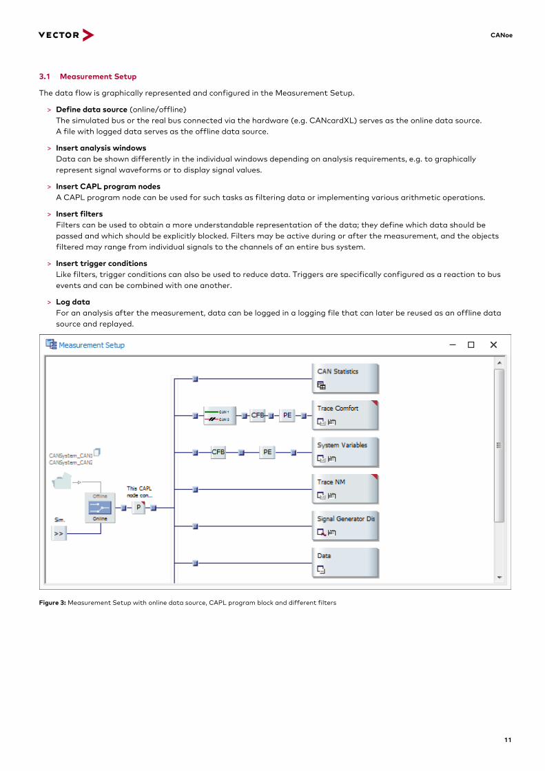
The data flow is graphically represented and configured in the Measurement Setup.

> Define data source (online/offline) The simulated bus or the real bus connected via the hardware (e.g. CANcardXL) serves as the online data source. A file with logged data serves as the offline data source.

> Insert analysis windows Data can be shown differently in the individual windows depending on analysis requirements, e.g. to graphically represent signal waveforms or to display signal values.

> Insert CAPL program nodes A CAPL program node can be used for such tasks as filtering data or implementing various arithmetic operations.

> Insert filters Filters can be used to obtain a more understandable representation of the data; they define which data should be passed and which should be explicitly blocked. Filters may be active during or after the measurement, and the objects filtered may range from individual signals to the channels of an entire bus system.

> Insert trigger conditions Like filters, trigger conditions can also be used to reduce data. Triggers are specifically configured as a reaction to bus events and can be combined with one another.

> Log data For an analysis after the measurement, data can be logged in a logging file that can later be reused as an offline data source and replayed.

Figure 3: Measurement Setup with online data source, CAPL program block and different filters

CANoe

12

3.2 Trace Window

Bus activities − such as the sending of messages or Error Frames − are listed in the Trace Window. Individual signal values may be displayed for each message. Functions such as those listed below are available for analyzing the data:

> Insert filters There are various types of filters in the Trace Window. They can be used to reduce the amount of data displayed, and data can even be deleted from the data stream.

> Hide unchanged data To improve ease of viewing, data that does not change is slowly faded or removed entirely from the screen.

> Color events Important events and messages can be highlighted in color.

> Set markers Markers can be set to identify and quickly find events. The marker is assigned to an event and therefore to its time stamp as well. The set markers can also be displayed in other analysis windows.

> Show statistics Various aspects of messages/signals, including their values, can be displayed in different views in detail. Differences between the time stamps or signal values may also be calculated.

> Log data It is possible to export some or all of the Trace Window contents. Files that have already been exported can be converted to a different format afterwards, e.g. to further process the same dataset in different programs.

Figure 4: Trace Window with active Stop filter and set marker

CANoe

13

3.3 Graphics Window

The Graphics Window is used to graphically display the values of signals, environment data and diagnostic parameters as curves. Listed below are some of the functions available for measurement and evaluation of these curves:

> Show measurement markers/difference markers Measurement or difference markers can be used to perform absolute or relative analyses of measurement values. The measurement marker can be synchronized to the Trace Window display.

> Set markers Markers can be set to identify and quickly find events. The marker is assigned to one event and therefore to its time stamp as well. The set markers can also be displayed in other analysis windows.

> Show measurement columns In the legend, global or local minima and maxima may be shown for each signal, or Y-differences between signals of the same type can be displayed.

> Show statistics Statistical data such as minimum, maximum, mean value and standard deviation can be compiled for selected signals or all signals of the Graphics Window.

> X/Y mode By right clicking in the signal list every signal can also be configured as x-axis.

> Log data Signals of the Graphics Windows can be logged automatically or manually during the measurement. This involves extracting the signals from the messages and saving them in binary form in signal based MDF files. In the Graphics Window, the entire signal waveform or just a visible section of the signal waveform can be saved to a file.

Figure 5: Graphics Window with set marker

CANoe

14

3.4 Scope Window

The Scope Window graphically depicts bus level measurements and is used for the analysis of protocol errors (see also option .Scope, Chapter 12 ).

> Set triggers In the Scope Window, it is possible to trigger manually, via CAPL or via preconfigured conditions. Any number of trigger conditions may be created, and the individual trigger conditions can be combined in a logical OR relationship.

> Analyze measurement values The diagram graphically depicts the measurement values and their logical interpretation.

> Compare signals The user may choose different approaches to comparing data. For example, it is possible to compare different time-based sections of the same data acquisition or time-based sections of different data acquisitions.

> Log data Acquired data may be exported and then imported for later analysis.

> CAPL control in test modules The Scope Window can be controlled from a CAPL test module. It can be triggered by CAPL, for example, or it can wait for a scope event to occur.

> Measurement Cursors A measurement cursor is useful to measure physical data like time and voltage as well as measuring the difference of these values related to another cursor. Cursor tooltips show the logical values (e.g. dominant/recessive) of bits. All physical values are listed in a separate legend.

> Global Markers In the Scope Window, markers can be set for marking significant points of a measurement. Each marker has a name and a defined time stamp.

> Eye diagram Enhanced analysis possibilities e.g. superposition of bits or presentation of the “ideal bit”.

Figure 6: Scope Window with eye diagram

CANoe

15

3.5 Data Window

The Data Window is used to display the values of signals, system variables and diagnostic parameters in different types of representation.

> Show values The data may be displayed as raw or symbolic values. Other display variants are scientific notation and the display of global and local min/max values.

> Log data Signals can be logged during the measurement and saved to MDF binary format.

Figure 7: Data Window with various representation types for incoming values

3.6 Statistics Window

The Statistics Window shows statistical information about bus activities (CAN, LIN, FlexRay) during a measurement. This includes such information as bus load on node and frame level, burst counter/duration, counters/rates for frames and errors, and controller states.

> Show statistical data of individual channels The display of statistical data can be limited to a specific channel, or it can be configured for all available channels.

> Set updating interval This is used to modify the interval for updating the display.

> Pause statistics The display of statistical data can be paused during a measurement.

CANoe

16

Figure 8: CAN Statistics Window with statistical data for one channel (CAN 2)

Certain CAN/LIN/FlexRay statistics can be evaluated in analysis windows such as the Graphics Window, or in program nodes via automatically defined statistical system variables. These system variables are available for each configured network channel and are updated independently of the Statistics Window.

3.7 State Tracker

The State Tracker can be used to analyze states, state transitions, CAN/CAN FD Frames, signals and diagnostic parameters to visualize time dependencies. The State Tracker is especially well-suited to displaying digital inputs and outputs as well as status information such as terminals status or network management states.

> Search for errors Errors can be searched and functions can be monitored based on analysis of the time response of states, signals and state transitions.

> Analyze information Various information such as the states of internal ECU communications, bus signals or ECU I/Os can be analyzed together.

> Monitor AUTOSAR runnables Monitoring of runnable states that were read out via XCP.

> Set triggers Users can define trigger conditions for initiating a measurement.

> Set markers Markers can be set to identify measurement time points. The time between the set markers can be measured.

CANoe

17

Figure 9: State Tracker for analyzing ECU states

3.8 Write Window

The Write Window displays system messages and user-specific outputs from CAPL programs.

> Configure output The Write Window offers different views for filtering system messages according to their source.

> Log output The Write Window output may be saved to a file or copied to the clipboard as text and be copied to other Windows applications from there.

> Status Display Informs about new unread warning and error messages in the Write Window.

Figure 10: Write Window with system messages and CAPL outputs

CANoe

18

3.9 Video Window

The Video Window can be used to record and play back video files.

The most commonly used video formats are supported in the Video Window depending on the current system configuration and the DirectShow components already installed on the system. Thus, for example, uncompressed AVI, compressed AVI (with corresponding installed Codec, e.g., DivX), MPG, MPEG, WMV, and MP4.

> Online measurement and recording Using a Video Window, video files can be recorded from a configured video source (e.g., a camera). After the measurement, the Video Window displays the recorded video file, which can be played back and navigated in.

> File import Outside of the measurement, it is possible to import video files to a Video Window.

> Offline analysis Define a video file as an offline source in the configuration of the Video Window. This video file is then displayed during the offline analysis. Typically, the video file that was recorded during the online measurement is defined as the offline source.

> Window synchronization Video files can be synchronized with other analysis windows.

Figure 11: Video Window

CANoe

19

3.10 GPS Window

The GPS Window can be used to integrate GPS information in CANoe. The GPS Window is part of the basic feature set of CANoe.

> Display data GPS data can be displayed in analysis windows.

> Offline analysis GPS data can be logged and replayed for later analysis.

> Window synchronization GPS data can be synchronized with other analysis windows.

> Display card The momentary vehicle position and trip route covered are displayed on an electronic map in the GPS Window. This enables consideration of geographic aspects in the interpretation of logged measurement data.

Figure 12: GPS Window

3.11 Triggers and Filters

Triggers and filters can react to specific bus events, and they serve to reduce the amount of displayed or logged data. Examples of trigger conditions are error states, messages, signals and signal changes (edges). Complex system states can be triggered by forming groups and linking them with logical operators.

> Filters in the Measurement Setup Various filters are available in the Measurement Setup that can be used to define which data should be passed to the specific analysis windows and/or which data should be explicitly blocked. All filters can be used as Stop and Pass Filters.

> Triggers in the Measurement Setup Different trigger conditions can be used in the Measurement Setup to influence the logging of data to a logging file.

> Filters in the Trace Window In the Trace Window, data can be reduced for analysis both during and after the measurement using various filters. For example, you could set predefined filters to filter for individual signals and signal values or set different column filters.

> Filter in the hardware The CAN controllers use acceptance filtering to control which received messages are passed to CANoe.

CANoe

20

3.12 Logging/Replay

Data can be logged in CANoe and replayed later in a post-measurement analysis.

> Replay The Replay Block can be used to replay measurement sequences that have been logged in a logging file. The messages contained in the logging file are introduced into the data flow.

> Logging The Logging Block can log the bus traffic in the BLF and ASCII formats. The logged data can then be replayed in offline mode or with a Replay Block.

4 Stimulation/Simulation

In developing distributed communications systems with CANoe, the remaining bus simulation is automatically created based on database information, including the graphic user interface for control and display. The communications behavior of these systems may be fully simulated and analyzed. Over the further course of the development process, individual nodes can be replaced by real ECUs within the simulation. This remaining bus and environment simulation gives the supplier a development and test environment for both the overall system and for individual ECUs and modules.

Phase 1 Phase 2 Phase 3

Figure 13: Development process with CANoe from network simulation to real overall system

Highlight

> Simple starting and stopping of simulation and stimulation features via status bar

4.1 Variables and Generators

System variables are available for all simulation and analysis blocks, panels and for the integrated I/O hardware. They are used system-wide to exchange configuration parameters, measurement values or to link external programs via the COM interface.

To stimulate the remaining bus simulation or connected I/O hardware, signals, environment or system variables can be directly introduced by Signal Generators. This makes it easy to inject signal curves such as ramps or sinusoidal waveforms into the system. It is also possible to extract logged signal waveforms from logging files and use them as the generator type.

4.1.1 Interactive Generator

The Interactive Generator (IG) can be used to send messages as well as to set the corresponding signal values. This is an easy way to create a remaining bus simulation.

> Define messages Messages can be defined manually in the send list or with a database. The properties of the messages can be customized.

> Send messages Messages which are configured in the send list can be sent periodically when a specific screen button is pressed or by pressing a predefined keyboard key.

CANoe

21

> Change signal values In the Interactive Generator, the raw data of each message can be modified in the signal list. For configured signals of a specific message signal waveforms (signal curves) may be defined with the integrated Signal Generator. Raw data and signal values can be easily sent with the associated message, e.g. to check the reaction of an ECU.

> Layer 7 protocols Depending on the bus system the Interactive Generator supports simple layer 7 protocols (e.g. J1939 or GMLAN) and the transmit of multiplexing messages.

Figure 14: Interactive Generator with configured messages and their signals

4.1.2 Signal Generator

The Signal Generator can be used to define a waveform for signals and variables (sine, ramp, pulse, value list, etc.).

> Send values Here, sending of the relevant messages is handled according to a defined send model. In LIN and FlexRay, a schedule table handles sending of messages. In CAN, the interaction layer (IL) handles sending of messages in conjunction with function libraries (DLLs). The Signal Generator can be started and stopped during the measurement.

> Define value waveforms There are two ways to define Signal Generators. A waveform may be defined for a single signal/variable, or it may be loaded from a logging file.

> Support in panels To automatically stimulate ECUs from panels over a longer time period, Signal Generators may be assigned to the signals/variables. The assigned Signal Generators are visualized on the panel and any errors are shown.

CANoe

22

Figure 15: Signal Generator with user-defined signal waveform

4.2 Set Start Values

In the Start Values Window, values that are set on measurement start can be preassigned for system variables, environment variables, and signals.

The list of start values can be exported to a file and loaded from a file. Thus, for example, simulation parameters can be conveniently assigned using various sets of start values.

Figure 16: Start Value Window

CANoe

23

4.3 Symbol Mapping

Using the mapping dialog, symbols (system variables, environment variables, and signals) can be mapped.

When the value of a source variable changes during measurement, the value of the destination variable is automatically set. Optionally, you can apply a linear conversion formula.

Figure 17: Symbol Mapping dialog

4.4 Interaction Layer, Network Management, Transport Protocols

CANoe offers an extensive set of protocol libraries for creating the remaining bus simulations. They implement such functions as network management based on a specific OEM or AUTOSAR standard. The use of standardized transport protocols simplifies the process of setting up simulation or test applications, because these services are already fully integrated. Other options may also be used to reproducibly inject error cases to check the related ECU stack. The interaction layers which are also available are used to abstract the sending behavior of the simulation nodes to a signal layer. This makes it easy to set signals in all applications, and CANoe then ensures that they are sent on the bus according to the OEM-specific sending logic.

CANoe supports the following protocol standards:

> Diagnostic protocols: KWP2000 and UDS (ISO 14229)

> Network management (NM): AUTOSAR, OSEK-NM

> Transport protocols (TP): ISO/DIS 15765-2, CMDT (J1939), BAM (J1939) and TPs for MOST, LIN and FlexRay

> Interaction layer (IL): Vector IL

4.4.1 OEM-Specific Extensions

Currently, CANoe also supports specific TP, NM and IL extensions for 20 OEMs that include BMW, Daimler, VAG, Audi, Ford, Toyota, Fiat, Porsche, Renault.

These extensions make it easy to generate an entire remaining bus simulation, including NM and TP. This also eliminates manual writing of code – e.g. for the send model. Serving as the basis here is a correctly parameterized network description file, in which the entire sending behavior is configured, and it also defines such information as which nodes participate in NM. The Model Generation Wizard can now generate an entire remaining bus simulation for CANoe from such a description file.

Please contact your Vector sales partner for more information.

CANoe

24

4.4.2 Configuration of the Interaction Layer

Configuration of the Interaction The configuration dialog of the Interaction Layer (IL) offers a straightforward way to display and edit transmission types.

The dialog evaluates the transmission type description of an interaction layer (Vector Interaction Layer, OEM Interaction Layer) from the database and displays it. The OEM-specific variants are taken into consideration here.

Figure 18: Configuration dialog of the Interaction Layer

4.5 MATLAB/Simulink

Development engineers use the CANoe MATLAB/Simulink integration for functional and application prototyping, integrating complex MATLAB models in CANoe tests and simulations and for developing control algorithms in real-time applications. CANoe and the Simulink models communicate directly via signals and system variables.

The CANoe MATLAB/Simulink integration supports three different execution modes:

> In the HIL or online mode, code is generated from the Simulink model that is added as a DLL at a simulated node in CANoe. The model is calculated in real time with CANoe. Automatically generated system variables can be used to make post-run changes to model parameters without recompiling.

> In offline mode, the two programs are coupled. Simulink provides the time base, and CANoe is in Slave mode. The entire system operates in simulated mode. It is not possible to access real hardware here.

> The synchronized mode is similar to offline mode in its operation. However, in synchronized mode CANoe provides the time base that is derived from the connected hardware. This enables access to real hardware in this mode. One limitation is that the Simulink model must be computed faster than in real time, because in this mode the Simulink simulation is slowed down to adapt the overall simulation to the CANoe simulation time.

CANoe

25

4.5.1 Further Functions of the CANoe MATLAB/Simulink Integration

> The Model Viewer depicts the integrated Simulink models and Stateflow diagrams, which gives precise insight into the model structure without MATLAB. It lets users navigate through the model structure.

Figure 19: Model Viewer

> To modify model parameters, the model can be calibrated over XCP on CAN or XCP on Ethernet while the model is running autonomously in standalone mode. This involves generating an A2L file in code generation.

Figure 20: Workflow calibration

CANoe

26

> Call of CAPL functions from a Simulink model

> Trigger a Simulink subsystem with a CAPL function

> React to changes to environment variables in Simulink

> Use of Simulink models in CANoe’s analysis branch. Special options for Simulink data analysis can be used here.

4.5.2 Further Information

The application note AN-IND-1-007_Using_MATLAB_with_CANoe describes the use of MATLAB/Simulink together with CANoe. It presents the fundamentals of the CANoe/MATLAB Interface and provides an overview of different use cases.

5 Test

5.1 Testing ECUs and Networks

One of the primary use cases of CANoe is to test ECUs and networks. Such tests are used to verify individual development steps, test prototypes or perform regression and conformance tests. CANoe services the System Under Test at all interfaces here. This assures the fullest possible test coverage.

Figure 21: Testing with full access to the ECU

CANoe

27

To assure that your testing tasks can be implemented simply and flexibly, the Test Feature Set consists of the following components:

> In CANoe, sequential test flows are implemented as test units or test modules, which are subclassified into test groups and test cases. The individual units/modules can be executed at any time during a measurement.

> Test units comprise a collection of data which contain the implementation of the tests (e.g. CAPL/C# files, test tables, test diagrams or parameter files). A test unit may contain for example the test implementation for a specific ECU function. Test units are managed within test configurations. A test configuration may contain 1…n test units which are sequentially executed in a consecutive manner. A CANoe system configuration on the other hand may contain any number of different test configurations which may be executed in parallel. Executable test units are developed with vTESTstudio. vTESTstudio is a separate product which provides the following concepts for efficient test design and organization:

> Different design methods for test implementation: tabular-based, programmatic (e.g. CAPL, C#) and graphical (e.g. Test Sequence Diagram, State Diagram)

> Parameter & Variant Management

> Classification Trees for efficient test data generation

> Project internal and external libraries for high reusability

> Traceability and change tracking of external requirements and test case specifications

> Add-on tools for connection to external test data management tools (e.g. IBM Rational Quality Manager, PTC Integrity, Siemens Polarion) including upload of the test results

> Test modules may be implemented in XML, CAPL or .NET. In XML modules, tests are assembled from predefined test patterns, and it is easy to parameterize them via input and output vectors. CAPL and .NET test modules, on the other hand, are programmed and therefore exhibit very flexible test flow control. The .NET test modules can be conveniently developed in C# or VB.NET. The different description forms may be combined according to requirements. Test modules are managed in test environments. These test environments contain test modules as well as further function blocks for test execution. Test environments are saved separately from the CANoe system configuration. Therefore, it is easy to reuse them in different projects. Hint: Test modules should only be used in the context of smaller test packages or for the quick examination of single functions of the subject under test. For all other use cases, the organization in a vTESTstudio project is recommended, where the tests can be designed and managed very effectively.

> In parallel to test execution, other system states can be checked such as conformance to the cycle times of individual messages. These constraints are automatically added to the test evaluation.

> The Test Service Library contains a collection of prepared test functions that simplify the process of setting up tests. They are used in the test modules and are parameterized via the database. For example, it is possible to monitor the cycle times of messages, an ECU’s reaction time from the time a message is received until it sends the response message or the validity of signal values and diagnostic parameters. To evaluate the quality of the tested ECUs, different statistical values of the tests are output, such as the number of reported deviations over the test time period.

> When a test module or test unit is executed, an extensive test report is generated. Along with the names of the executed test cases and the individual test results, user-defined information or automatic screenshots of various analysis windows can also be recorded, for example. The following output formats are available for the test report:

> VTESTREPORT (recommended) CANoe writes the results in a very efficient file format that enables users to perform fast and comprehensive analysis. The created VTESTREPORT files can be visualized and analyzed later on with the CANoe Test Report Viewer. This tool is part of the CANoe installation, and can be obtained from the Vector download center for usage without additional costs.

> XML CANoe writes the results to a flexibly further processed XML file. The output format for the test report is adapted into a readable file via an XSLT stylesheet.

CANoe

28

> Direct control of I/O hardware in CANoe makes it possible to use analog and digital ECU interfaces in addition to bus communications. Along with standard I/O components, the Vector VT System represents a modular hardware system for comprehensively testing ECUs in the automotive field.

Figure 22: Graphical test design for a central locking system in vTESTstudio

CANoe

29

Figure 23: Test flow for a central locking system with associated test report in HTML

Figure 24: Graphical user interface of the new CANoe Test Report Viewer

CANoe

30

5.2 CANoe RT/VN8900 and CAPL-on-Board

CANoe offers different options for executing real-time relevant simulation and test functions on a dedicated platform, i.e. separate from the graphic user interface. This simply involves increasing total system performance as necessary, and it is possible to implement shorter latency times and more precise timers.

> In CANoe RT, the simulation and test environment and evaluation are configured on a standard computer, while the simulation and the test run on a dedicated computer under Windows Embedded.

> The network interface VN8900 contains a processor platform, on which the simulation and the test are automatically executed.

> With the VN8900 it is possible to download a CANoe configuration onto the device and operate it without in a standalone mode without GUI computer.

> CAPL-on-Board improves the real-time capability of Vector USB hardware interfaces e.g. VN1630/40, by allowing CAPL nodes and Visual Sequences to run directly on the hardware.

Figure 25: Test system based on CANoe RT and Test Feature Set with integration of different bus systems as well as digital and analog I/Os

5.3 Vector Tool Platform

The Vector Tool Platform (VTP) offers various services that can be used in CANoe. Currently VTP consists of the two components Smart Device Access (SDA) and Extended Real Time (ERT). Not all devices support all components automatically.

> Extended Real Time improves the latency and determinism of CANoe. To achieve this, the device is logically divided into two areas. A new area provides Extended Real Time, in which predefined functions can be executed under real-time conditions. With ERT, additional transfer cycle times of 200µs and 500µs can be set for some measured values in order to achieve higher sampling rates.

> The Platform Manager is an add-on tool for configuring and controlling all devices of the Vector Tool Platform (VN8800, VN8900, VT6000, RT Rack).

Figure 26: Vector Tool Platform components

5.4 CAN/CAN FD Disturbances

With the hardware interface VH6501 the CAN / CAN FD bus can be disturbed. The hardware combines the functionality of a faulty hardware and a network interface in one device.

For triggering the disturbance, the interface provides various triggering possibilities for CAN and CAN FD, e.g.

> I / O trigger

> Frame trigger, e.g. SOF, Frame, Bus Idle, Error

> Combined Frame Triggers for disturbing e.g. different IDs (up to 32 parallel conditions including wildcards)

CANoe

31

Any interfering sequences can be generated fine granular, e.g. to put the controller in the BUS-OFF state or to perform a sample point test.

Disturbing dominant levels with recessive levels are also possible

Figure 27: Disturbance of the ACK slot at a CAN frame recorded with option .Scope

The VH6501 can be configured in CANoe with a built-in CAPL API. Different triggers and sequences can be configured with this API. The trigger position for a disturbance sequence may be set arbitrarily for a frame trigger.

Figure 28: CAPL code definition and activation of the ACK slot fault

The CAPL API offers the possibility to use the VH6501 very well in an automated test.

Various fault situations can be generated on the CAN/CAN FD bus, e.g.:

> bit errors

> defects in shape

> lengthening and shortening of bits

> CRC errors

5.5 Further Information

Fundamental concepts of CANoe’s Test Feature Set are described in application note AN-IND-1-002_Testing_with_CANoe.

CANoe

32

6 Diagnostics

CANoe is used in diagnostics development in ECUs. In this area, CANoe supports both the implementation and testing of diagnostics functionality by providing access to the diagnostic interfaces of ECUs. The following concepts and functions are available, for example:

> Support of all important diagnostic description formats for KWP2000 and UDS (ISO 14229):

> ODX 2.0.1/2.2.0 as PDX files

> MDX 2.0/3.0/4.0

> CANdelaStudio (CDD)

> Option of modifying key diagnostic communication parameters of the diagnostic description (transport and diagnostic layer) in the Diagnostic/ISO-TP configuration dialog

> Basic Diagnostic Editor for quickly defining simple diagnostic services, if no diagnostic description is available (for CAN, LIN, FlexRay, Ethernet and K-Line)

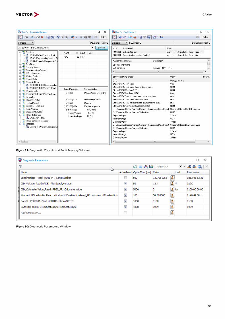
> Interactive diagnostic tester with Diagnostic Console, Fault Memory Window and Diagnostic Session Control with configurable security-DLL

> Interactive Diagnostic Parameters Window for cyclic or manual query and display of diagnostic parameters from diagnostic responses

> Preconfigured OBD-II tester with related Diagnostic Console and Fault Memory Window

> Support of several addressing schemes (e.g. normal, extended, normal fixed and mixed) and addressing types (functional/physical)

> Analysis of diagnostic communications on the service and parameter levels (i.e. symbolic representation based on the diagnostic description) in the Trace, Data and Graphics Windows as well as in the State Tracker

> Display of protocol errors in the Trace Window

> Optional use of panels to display diagnostic parameters and stimulation of ECUs via diagnostic requests

> Simulation of the diagnostics functionality of ECUs

> Specification/integration/regression tests based on the Test Feature Set (Test Units, CAPL and XML test modules) or with CANoe .DiVa

> Options for accessing all diagnostic communication layers (CAN messages, transport protocol and diagnostic services) for good and bad case tests

> Support of all important network types in the automotive field (CAN, LIN, FlexRay, Ethernet and K-Line)

> Gateways to other networks (e.g. MOST) can be implemented by CAPL simulation nodes or CAPL DLLs

> Support of DoIP (Diagnostics over IP), HSFZ (High Speed Fahrzeugzugang) and DoSoAd (Diagnostics over AUTOSAR Socket Adaptor)

> Logging and replay of diagnostic sequences via macros

CANoe

33

Figure 29: Diagnostic Console and Fault Memory Window

Figure 30: Diagnostic Parameters Window

CANoe

34

Figure 31: Basic Diagnostic Editor

Figure 32: OBD-II Window

CANoe

35

Figure 33: Diagnostic/ISO-TP configuration dialog

Figure 34: Representation of diagnostic communication in the Trace Window

6.1 Further Information

The application note AN-IND-1-001_CANoe_CANalyzer_as_Diagnostic_Tools describes a general introduction to working with diagnostics in CANoe/CANalyzer. Fundamental technical aspects and options are presented with the Diagnostic Feature Set. This document supplements CANoe’s online help and can be used as a tutorial.

The application note AN-IND-1-004_Diagnostics_via_gateway_in_CANoe describes the concept for a diagnostic gateway between CAN and every other bus system or transport protocol, to make CANoe’s Diagnostic Feature Set available if direct access is not possible.

CANoe

36

7 SoA and AUTOSAR Adaptive

7.1 Communication Concepts – Current Developement

The classic signal-based communication is increasingly supplemented by service-oriented communication patterns. The AUTOSAR Adaptive platform, for example consistently uses service-oriented approach. Service-oriented communication is often based on the TCP/IP protocol stack and uses communication middleware, for example SOME/IP. The transmitted network message, i.e. the Ethernet frame, and the actual application view drift here much more apart than in case of signal based communication via CAN. In addition, the service interfaces and the associated data structures are defined in a way which is detached from a specific network transmission or network topology.

7.2 The CANoe Communication Model

CANoe supports this new design paradigm. To do so, databases are imported into the CANoe communication model. Via a built-in Communication Object Editor you can define your own communication objects and edit the existing ones.

Figure 35: Import options for the CANoe communication model.

CANoe enables the use of the service interfaces directly as modeling artifact. The service interfaces support methods and events. Complex data types, used for example in the area of object detection, are supported directly. Endpoints which provide or use a service interface (providers and consumers) can be directly simulated in CANoe.

CANoe

37

Figure 36: Access of service interfaces and representation in the Trace Window.

8 Programming

8.1 CAPL Interface

The CAPL (Communication Access Programming Language) programming language extends the functional scope of CANoe tremendously. Special characteristics of CAPL include:

> Can be learned quickly since it is based on the C programming language

> Fully event-controlled in its operation. CANoe assumes control.

> Supports symbolic access to all database information such as messages and signals. Signal values can be used directly in their physical form.

> The language has been extended with special functions for quick implementation of problem solutions in various use scenarios (simulation, testing, diagnostics and analysis of various bus systems)

> Flexible extension by external libraries

8.1.1 C-Like Syntax

The usual scalar data types and arrays are provided (1, 2, 4 and 8 byte long whole number types as well as an 8 byte long floating point type). Assignments, arithmetic operators and loop flow control conform to C-syntax.

myFunction {

int counter;

for ( counter = 0; counter < 8; counter++ ) {

doSomethingWithCounter ( counter );

}

}

CANoe

38

8.1.2 Event-oriented Control

CAPL is an event-controlled programming language. In contrast to C, special predefined event handlers (event procedures) are available in CAPL, which are always executed whenever a specific event occurs – or, if time controlled, then triggered by the hardware or internal to CANoe.

Here are just a few examples of these event handlers:

Event Handler Event

On timer seconds cycle Time controlled

On message ESPStatus Message input or output

On signal update Rewrites signal value

On sysvar Modifies system variable

On diagRequest Diagnostic request

On FRError Detects FlexRay bus errors

8.1.3 Symbolic Access

Signal values are generally accessed as physical values, regardless of the scaling of message transmission. This is set in the database and is taken from there.

> Physical access to signal values:

// Definition of the representation in the database

$EnergyMgmt::BatteryVoltage = 14.1;

> Access to raw value of a signal:

// 8 to 18 Volt with 12bit resolution, without range check

$EnergyMgmt::BatteryVoltage.raw = (14.1 - 8) / (18 - 8) * 4096;

> Access on a message base:

// Most significant bytes Motorola, of 12 bits only the lower 4 bits are used

msg.byte(0) = (msg.byte(0) & 0xF0) | (byte)((14.1 - 8) / (18 - 8) * 4096 / 256) & 0xF;

// Least significant byte

msg.byte(1) = (byte)((14.1 - 8) / (18 - 8) * 4096) & 0xFF;

output(msg);

8.1.4 Application-Specific Language Extensions

For all use cases of CANoe there are numerous functions that are specially tailored to everyday problems related to these topics.

> Simulation A complete remaining bus simulation can be created with the help of CAPL. This relieves the developer of routine work tasks. Signals, messages and the timing behavior of the buses are defined in the database (e.g. in DBC, LDF or FIBEX files); these files are often managed, maintained and updated centrally. Using the supplied extensions (node layer DLLs), the database information can be used without having to write a single line of code. Sending, for example, - periodic sending or just on specific events – is handled entirely by CANoe according to database requirements, and the developer only needs to be concerned with the actual functionality, i.e. the contents of signals.

> Testing CAPL also offers convenient control options for programming automated tests that support both test execution and evaluation. Just a few lines of code is all it takes to create a basic structure that utilizes the test flow and automated reporting. So, with just a small program, a CAPL test node is able to provide a well-organized summary of the test flow with the standard report.

CANoe

39

testcase MyTestCase()

{

TestCaseTitle("myTC", "My Test Case");

TestCaseDescription("A test of mine");

TestCaseComment("first take a short break ");

TestWaitForTimeout(200);

If ( MyTestExecution () > 0 )

TestStepPass("myTC successful");

else

TestStepFail("myTC failed");

}

long MyTestExecution ()

{

/* Own code */

return 1;

}

MyTest() {

MyTestCase();

TestSetVerdictModule(TestGetVerdictLastTestCase());

}

Figure 37: Test node with Test Execution dialog and test report

CANoe

40

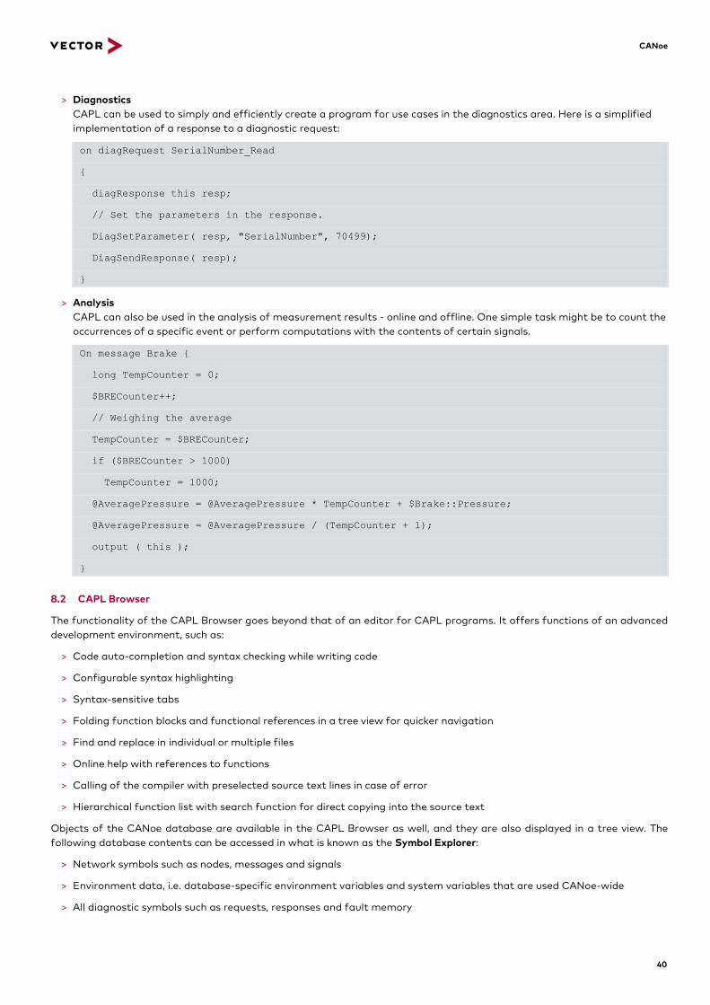
> Diagnostics CAPL can be used to simply and efficiently create a program for use cases in the diagnostics area. Here is a simplified implementation of a response to a diagnostic request:

on diagRequest SerialNumber_Read

{

diagResponse this resp;

// Set the parameters in the response.

DiagSetParameter( resp, "SerialNumber", 70499);

DiagSendResponse( resp);

}

> Analysis CAPL can also be used in the analysis of measurement results - online and offline. One simple task might be to count the occurrences of a specific event or perform computations with the contents of certain signals.

On message Brake {

long TempCounter = 0;

$BRECounter++;

// Weighing the average

TempCounter = $BRECounter;

if ($BRECounter > 1000)

TempCounter = 1000;

@AveragePressure = @AveragePressure * TempCounter + $Brake::Pressure;

@AveragePressure = @AveragePressure / (TempCounter + 1);

output ( this );

}

8.2 CAPL Browser

The functionality of the CAPL Browser goes beyond that of an editor for CAPL programs. It offers functions of an advanced development environment, such as:

> Code auto-completion and syntax checking while writing code

> Configurable syntax highlighting

> Syntax-sensitive tabs

> Folding function blocks and functional references in a tree view for quicker navigation

> Find and replace in individual or multiple files

> Online help with references to functions

> Calling of the compiler with preselected source text lines in case of error

> Hierarchical function list with search function for direct copying into the source text

Objects of the CANoe database are available in the CAPL Browser as well, and they are also displayed in a tree view. The following database contents can be accessed in what is known as the Symbol Explorer:

> Network symbols such as nodes, messages and signals

> Environment data, i.e. database-specific environment variables and system variables that are used CANoe-wide

> All diagnostic symbols such as requests, responses and fault memory

CANoe

41

Figure 38: CAPL Browser with opened CAPL program, contained event procedures and network symbols from the database

8.3 .NET Programming

In CANoe,.NET programming languages can be used at different places:

> for programming simulated network nodes

> for programming test modules, test cases and test libraries

> for programming of so called snippets

CANoe offers a special API for.NET programming, which specifically extends the languages (i.e. it creats Embedded Domain Specific Languages). Programming languages that are directly supported are C# (programming language recommended by Vector), Visual Basic .NET and J#:

> Use Visual Studio as editor .NET programs can be conveniently edited, e.g. with Visual Studio 2005, 2008 or 2010 as the development environment. The Express Editions of Visual Studio are available free of charge.

> Access to signals, environment and system variables A class is provided in .NET for each signal and each environment or system variable; it can be used to access the value in the CANoe run-time environment. Example:

double value = EnvSpeedEntry.Value;

CANoe

42

> Access to CAN messages A class is available in .NET for each CAN message defined in the database. Instances of these classes can be created, signal values can be set, and the frame can be placed on the bus with the Send method. In addition, the attribute [OnCANFrame] can be used to react to the receipt of CAN messages.

If no database is used, the general class CANFrame can be used directly, or individual classes can be derived from this class. Signals are defined with the attribute [Signal].

> Access to diagnostics If one or more diagnostic descriptions are configured, a .NET library can be used to send diagnostic requests and receive diagnostic responses in test modules and snippets. It is possible to set parameters in requests and read out from responses.

The library Vector.Diagnostics is supported by several other Vector applications, i.e. it is very easy to reuse diagnostic sequences in CANoe as well as in CANape, CANdito or Indigo.

> Event procedures Methods with special attributes are provided for reacting to events in CANoe. The methods are then called if the event occurs (exactly as in CAPL).

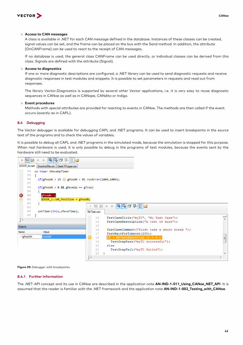
8.4 Debugging

The Vector debugger is available for debugging CAPL and .NET programs. It can be used to insert breakpoints in the source text of the programs and to check the values of variables.

It is possible to debug all CAPL and .NET programs in the simulated mode, because the simulation is stopped for this purpose. When real hardware is used, it is only possible to debug in the programs of test modules, because the events sent by the hardware still need to be evaluated.

Figure 39: Debugger with breakpoints

8.4.1 Further Information

The .NET-API concept and its use in CANoe are described in the application note AN-IND-1-011_Using_CANoe_NET_API. It is assumed that the reader is familiar with the .NET framework and the application note AN-IND-1-002_Testing_with_CANoe.

CANoe

43

8.5 Visual Sequencer

This is a quick way to graphically configure flow sequences without requiring programming. Variables and signals may be set within such sequences. Frames and diagnostic commands can also be sent. In addition, it is possible to wait for certain events, check values or define repetitions with control structures (repeat…until). These sequences are therefore ideal for simple tests of heterogeneous systems or for stimulating ECUs.

Figure 40: Visual Sequencer for creating test and stimulation sequences. Makes it easy to select commands and database objects with auto-complete support and to display detailed database information.

9 Panels

Panels are graphical elements that can be used to modify signal and variable values and display them with controls such as sliders or pointer instruments. Different types of panels are available in CANoe.

> Signal panel A signal panel offers a simple way to modify signal values at measurement time. A distinction is made between node panels and network panels among the signal panels. When a node panel is used, the Tx signals of the related node are automatically configured. When network panels are used, the Tx signals of the entire network are automatically configured.

> Symbol panel The symbol panel can be used to display and/or modify the values of signals and variables during the simulation.

> User-defined panels User-defined panels are user interfaces for special use cases. Such panels might be used to control the simulation and test environment, for example, or to display the analysis data from CAPL programs. The Panel Designer can be used to conveniently create such panels. For example, it is easy to link a symbol to a control by drag & drop. The individual panels and controls are configured via the constantly open Properties Window, and a whole series of useful alignment functions ensure an optimal layout.

> User-programmable ActiveX and .NET panels These panels that are created with programming languages such as Visual Basic 6.0, Visual Basic.NET or C# can be integrated in CANoe.

CANoe

44

Figure 41: User-defined panels for displaying signal and variable values

10 Hardware Interfaces

CANoe supports all hardware interfaces available from Vector. Optimal bus access is possible for every use case thanks to a large selection of different computer interfaces (PCMCIA, USB 2.0, PCI, PCI-Express, PXI) and bus transceivers.

Figure 42: Overview of Vector hardware

11 Interfaces to Other Applications

CANoe can access parameter values in existing ECUs using the ASAM-MCD3 Server provided by CANape − and thereby over XCP and CCP. Option .XCP offers direct XCP integration in CANoe (see chapter 13 ).

11.1 COM Interface

The integrated COM Server (Component Object Model) enables control of the measurement sequence by external applications and convenient data exchange with standard software, e.g. for measurement data analysis or in-depth evaluation of the observed bus traffic. Frequently used programming/script languages here are Visual Basic or Visual Basic for Applications. C++/C# are also frequently used. The functionality that CANoe offers over the COM interface covers such aspects as:

> Control of the simulation, starting and stopping the measurement

> Loading existing configurations, generating new configurations, adding databases and blocks to the Simulation Setup

> Control of automated tests, start test execution, add test modules

> Access to signals and system variables, access to CAPL functions, compiling of CAPL nodes

CANoe

45

Visual Basic script example for starting the measurement:

set app = createobject( "canoe.application")

set measurement = app.measurement

measurement.start

set app = nothing

Visual Basic script example for opening a configuration:

set app = createobject( "canoe.application")

app.open "D:\PathToMyConfig\myconfig.cfg"

set app = nothing

11.1.1 Further Information

A general introduction to COM Server functionality of CANoe/CANalyzer is described in application note AN-AND-1-117_CANalyzer_CANoe_as_a_COM_server. Fundamental technical considerations and options are presented, and they are illustrated as Microsoft Visual Basic examples.

11.2 FDX

CANoe FDX (Fast Data eXchange) is a protocol, with which data can be exchanged between CANoe and other systems − simply, quickly and with minimal delay − over an Ethernet connection. The protocol gives other systems read and write access to system variables, environment variables and bus signals of CANoe. It is also possible to send control commands to CANoe via FDX (e.g. for starting and stopping the measurement) or receive status information.

The other system might be an HIL system in a test bench, for example, or a computer that should display data from CANoe. The protocol is based on the widely used standard protocol UDP (based on IPv4).

11.3 ASAM XIL API

ASAM XIL is an API standard for the communication between test automation tools and test benches. All types of test benches are supported, e.g. SIL, MIL and HIL.

Data between CANoe and the test benches is exchanged by utilizing prepared .NET assemblies with a C# API.

11.4 FMI

FMI (Functional Mock-up Interface) is a tool independent standard to exchange models as well as to establish tool couplings. CANoe supports the import of such models (FMUs) for co-simulation as well as the export of FMUs. Both FMI 1.0 and 2.0 is supported.

12 Option .Scope

The option .Scope is an integrated oscilloscope solution for CANoe based on a very powerful USB oscilloscope hardware. This CANoe option appears as a further analysis window with views for configuration, bus level and protocol decoding. The supported hardware has up to 4 input channels for example 2 CAN / CAN FD / FlexRay or LIN 4 / IO channels can be measured. The scope is triggered by the Sync line of Vector interface hardware (e.g. VN1630/40, VN8900, VT System). The option .Scope is available for all variants except CANoe pex, and together with the CANoe Test Feature Set can be used to fully automate physical layer tests.

12.1 Application Areas

The powerful combination of the USB oscilloscope and CANoe offers many new ways to analyze protocol errors and to automate physical layer tests. The analysis of the bus system’s physical layer is often indispensable, especially when performing conformance tests. With bus-specific trigger conditions and CANoe time synchronization, the causes of protocol errors can be found significantly faster than with any traditional oscilloscope.

CANoe

46

Figure 43: Detailed analysis of a CAN FD frame/error on physical and logical level with the Scope Window

12.2 Overview of Advantages

> Extremely compact and portable oscilloscope solution based on an USB oscilloscope hardware

> Easy bus connection via Vector Scope Bus Probe

> Oscilloscope functionality specially developed for bus analysis, e.g.:

> Predefined trigger conditions for bus errors and events

> Synchronous recording of bus and I/O signals with the CANoe time base

> Complete decode of protocol errors (e.g. CAN Error Frames)

> Eye diagram

> CAPL interface for automated scope tests including report creation

12.3 Supported Protocols

> Bus systems: CAN, CAN FD, FlexRay und LIN

> Sensor protocols: SENT and PSI5

CANoe

47

12.4 Supported Oscilloscope Hardware

> Vector PicoScope 5444B-034:

> USB precision oscilloscope with 200 MHz bandwidth and 500 MS/s sampling rate

> 4 input channels for bus signals (2 CAN/CAN FD/FlexRay or 4 LIN/IO)

> Vector PicoScope 5242B-034:

> USB precision oscilloscope with 60 MHz bandwidth and 500 MS/s sampling rate

> 2 input channels for bus signals (1 CAN/CAN FD/FlexRay or 2 LIN/IO)

> Bus connection via Vector Scope Bus Probe with D-Sub connector

> Vector Scope Y-Trigger Cable for internal and external triggering via the sync line of a Vector interface

12.5 Oscilloscope Software

Option .Scope appears as a new analysis window in CANoe with views for configuration/measurements, bus levels and protocol decoding.

12.5.1 Configuration Functions

> Connection of several bus signals to input channels of oscilloscope. For each bus system a default configuration for scope hardware is created.

> Easy configuration of sampling rate (independent of bus baud rate) in min. sampling points per bit

> Automatic adjustment of acquisition time depending on the bus baud rate

> Pre-/post-trigger time adjustable from 10% to 90%

> Support of up to multiple scope devices of the same type

12.5.2 Trigger Functions

> Single and Repeated trigger modes

> Manual triggering via the toolbar or CAPL function

> Simple trigger conditions:

> Trigger on frames (ID or ID range)

> Trigger on protocol errors (e.g. CAN Error Frames)

> All conditions may be combined in a logical OR relationship

> Triggering on external signals with edge or pulse triggers (IO trigger)

> Advanced trigger conditions programmable by CAPL:

> Trigger on change in a frame signal or in a system variable (e.g. I/O)

> Trigger on test fail verdict in test modules

> Complex trigger conditions may be defined as AND/OR relationships

> Establishment of trigger conditions via the COM interface of CAPL

CANoe

48

12.5.3 Analysis Functions

> Detailed decoding of the bus levels on the bit level, even in case of protocol errors

> Display of the time stamp and the voltage value per sampling value

> Bidirectional synchronization of Trace view (logical values of the data link layer) and the diagram (physical values). The diagram shows the signal encoding of the Trace view.

> Time-Synchronization with other CANoe windows, e.g. Trace Window, Graphics Window and State Tracker

> CAPL:

> Serial bit mask analysis. Definition of bit masks for each bit in analysis range (CAN, CAN FD and FlexRay)

> Measurement functions for bus signal voltage and time difference (e.g. bit time)

> Measurement functions for rise/fall time of bit edges

> Test Feature Set (TFS) to establish automated and reproducible test scenarios with support of test reports

12.5.4 Offline Functions

Offline functions of the Scope Window are available to users even without a license for option .Scope, e.g. to view and analyze measurements made by colleagues.

> Overview and easy management of scope measurements

> Automatic display of new measurement data

> Eye diagram analysis with single bitmask accessible via user interface

> Export and import of the entire scope measurement with logical and physical data (binary format *.csfx)

> Export of scope measurement data in ASCII (*.csv) or MATLAB formats (*.mat)

> Export/Import of eye diagrams (*.ceye).

> Comparison mode for scope signals and for entire scope measurements

> Easy screenshot creation and bitmap export for test reports

> Marking significant points of a measurement with global markers

13 Option .Sensor

The option .Sensor allows you to analyze the sensor communication. It is possible to observe sensor signals on the sensor bus as well as the distribution of the sensor signal in the vehicle network. Even complex communication scenarios can be generated and analyzed quickly, as proven CANoe analysis concepts and an intuitive configuration are used. With the ability to simulate both the control unit and the sensor, option .Sensor also supports developers in building simple to demanding test environments. Full control over all relevant log data consists in the simulation. In addition, sophisticated error detection mechanisms facilitate the debugging of the system.

The physical connection to the sensor networks is done using the hardware module VT2710. It is fully adapted to the functionality of option .Sensor and part of Vector's modular test environment VT System. The flexible structure of the VT2710 is beneficial: as required, up to four PSI5 or SENT channels are configurable with piggybacks. With this module, users have a precise analysis tool, which allows accurate bitrate settings and precise message time stamps and fits in seamlessly into the existing VT environment with the tool concept as well as the programming interface. The module is prepared for additional sensor logs.

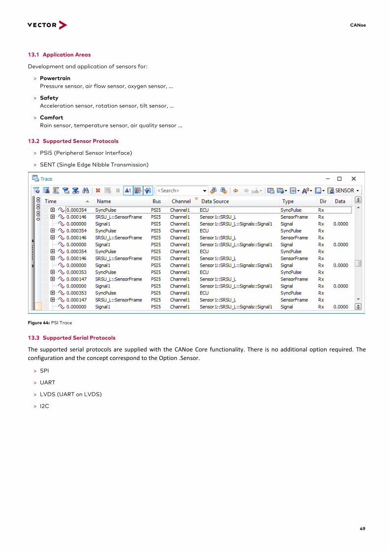
CANoe

49

13.1 Application Areas

Development and application of sensors for:

> Powertrain Pressure sensor, air flow sensor, oxygen sensor, ...

> Safety Acceleration sensor, rotation sensor, tilt sensor, ...

> Comfort Rain sensor, temperature sensor, air quality sensor ...

13.2 Supported Sensor Protocols

> PSI5 (Peripheral Sensor Interface)

> SENT (Single Edge Nibble Transmission)

Figure 44: PSI Trace

13.3 Supported Serial Protocols

The supported serial protocols are supplied with the CANoe Core functionality. There is no additional option required. The configuration and the concept correspond to the Option .Sensor.

> SPI

> UART

> LVDS (UART on LVDS)

> I2C

CANoe

50

13.4 Highlights

> Intuitive user interface for quick configuration of the sensor channels

> Sensor configurations can be comfortably exported for other CANoe configurations

> CANoe Trace Window for concise protocol analysis

> Serial hardware module VT2710 supporting four PSI5 or four SENT channels

Figure 45: VT Module 2710 and configuration dialog of the Option .Sensor

14 Option .SmartCharging

In order to test the complete Smart Charge communication the option .SmartCharging may be used. CANoe simulates either the vehicle (EV) or the charge point (EVSE). Just like with the other options a protocol analysis is easily possible, i.e. SCC specific events are displayed symbolically in the Trace Window. Furthermore there are a CAPL API as well as specific system variables available. The protocols ISO15118 and DIN70121 are supported. The option .SmartCharging requires the option .Ethernet. The specific VT System module VT7870 provides access to the hardware including fault injection.

CANoe

51

15 Option .AMD/XCP

Option .AMD/XCP extends CANoe by adding the ability to access ECU memory. This access is done via the ASAM-standardized XCP or CCP protocol and is convenient to configure with files in A2L format.

15.1 Application Areas

15.1.1 Calibration Protocol (XCP) / CAN Calibration Protocol (CCP)

CANoe offers access to internal ECU values via XCP/CCP for testing and analysis tasks. In contrast to the pure blackbox test, in which only the external ECU signals are stimulated and measured, internal values can also be calibrated and evaluated over XCP/CCP. Changes to these parameters lead to specific error states, and the resulting ECU behavior can be tested directly. It is also possible to test different variants of ECU software – switching is performed directly over XCP. Missing sensor values can also be simulated by writing values to the relevant memory locations via XCP/CCP.

In analysis, CANoe .AMD/XCP lets you analyze internal ECU parameters time synchronous to bus signals. For example, status information can be incorporated into the analysis, e.g. terminals status or task switching.

Figure 46: Access to an ECU via XCP on CAN/FlexRay/Ethernet and CCP-on-CAN

15.1.2 AUTOSAR Monitoring and Debugging (AMD)

Effective with release 10 the Vector MICROSAR AUTOSAR stack offers the generation of A2L files for the BSW modules (Basic Software Components) and the SWC (Software Components) and thereby provides the symbolic information.

You can read internal states and data flow out of a control unit and analyze it together with bus data. Option .AMD/XCP uses the established XCP and CCP protocols to read the data from the control unit.

Figure 47: Potential ECU access methods with CANoe .AMD

CANoe

52

15.2 ECU Access

15.2.1 Supported Bus Systems and Protocols

> XCP (X Calibration Protocol) on CAN, CAN FD, FlexRay2, Ethernet3 and LIN

> CCP (CAN Calibration Protocol)

15.2.2 VX1000 Measurement and Calibration Interface

> Measurement at rates of up to 30 MB/sec

> Supported debug interfaces: DAP (Device Access Port), Nexus Class 2 and 3

> No additional CPU load during measurement via Nexus Class 3 and DAP

> Capable of use in vehicles

> Interface via XCP on Ethernet

> Time stamp precision: 1µs

> Available for the following microcontroller: Infineon TriCore, Infineon XC 2000, Infineon Aurix, Freescale MPC5xxx, Texas Instruments TMS 570, Renesas V850 E2, others upon request.

Figure 48: Vector VX1000 product family

15.2.3 CSM Measurement Module

Via the XCP gateway module you can access the measurement data of high-precision measurement modules of the CSM company. For example, the measurement module ADMM 4 HS800 provides four analog measurement values with 800 kHz. You can evaluate and log these measurement data via the option .AMD/XCP.

15.2.4 Hardware Debugger Support

Hardware debuggers from the iSYSTEM company enable access to ECU memory without additional software or an XCP driver. No additional resources are utilized, and real-time behavior is unaffected.

> Interface via XCP on Ethernet Slave in winIDEA software version 9.12.78 or newer

> Measurement via pre-defined DAQ lists (Data AcQuisition):

> On change of a memory area (minimum cycle 100 µs)

> Periodically at 1 ms, 10 ms, 100 ms, 1 s

> Time stamp precision: 100 µs

> Universal solution for ECU development in the laboratory

2 Requires the corresponding CANoe option (.FlexRay/.LIN) 3 Display of Ethernet packets requires CANoe option .Ethernet. Transmitted data can be analyzed without option. Ethernet.

CANoe

53

15.3 Overview of Advantages

> Extended test options by access to internal ECU values

> Time synchronous analysis of internal ECU values, bus signals and I/O signals

> XCP/CCP protocol interpretation in the Trace Window (online and offline)

> Automatic configuration via ASAM A2L file

15.4 Functions

> XCP/CCP Window for configuration

> Online access to internal ECU values in RAM over XCP on CAN, XCP on Ethernet (TCP and UDP), XCP on FlexRay, XCP on LIN and CCP (for CCP/XCP on CAN, XCP on FlexRay and XCP on LIN the respective bus options are required.)

> Measurement methods: DAQ, Polling, on connect, Single Shot Upload over CAPL

> Writes scalar, multi-dimensional, and complex variables to the ECU's RAM via Download

> Measuring with ECU time stamp for DAQ

> Supports ASAM MCD-2 MC (A2L) databases up to version 1.7

> Support of scalar CCP/XCP data types (UBYTE, SBYTE, UWORD, SWORD, ULONG, SLONG, UINT64, SINT64, FLOAT32_IEEE, FLOAT64_IEEE)

> Complex CCP/XCP data types: 1-dimensional arrays, CURVE, MAP (supported axis types: COM_AXIS, SHARED_AXIS, FIX_AXIS)

> Dynamic, static and predefined DAQ lists are supported

> Secure access via Seed & Key (DLL and SKB format)

> Parallel access to multiple ECUs

> Address Update for ECU symbols from Linker Map file

> Address Update for ECU symbols from the ECU at runtime (generic measurement)

> XCP/CCP values are available as system variables in all CANoe functions

> Can be run under CANoe RT (Real Time) and VN8900 in standalone mode

CANoe

54

15.5 Integration in CANoe

CANoe assumes the role of the XCP/CCP master, which is to configure via one A2L file. The XCP signals are available as system variables; they enable access via the Test Feature Set, CAPL, .NET, DiVa, MATLAB/Simulink and CANoe analysis windows. The XCP signals are always located under the namespace <XCP>::<ECU name>. Here, “ECU name” stands for the name of the ECU to be measured, which is given in the XCP configuration. Based on this CANoe .AMD/XCP can address multiple ECUs over XCP in parallel.

Figure 49: System variable configuration in CANoe

Figure 50: XCP system variables in the State Tracker

15.6 Configuration

Option .AMD/XCP is configured by the A2L file format standardized by the ASAM working group. The A2L file contains information about communication (transport layer) with the ECU and descriptions of the variables that can be measured and stimulated. It also contains information about the interpretation of values (symbolic value tables) and conversion rules, so that symbolically interpreted values can be displayed directly in CANoe’s analysis windows.

CANoe

55

16 Functional Extensions for Special Applications

16.1 DiVa (Diagnostic Integration and Validation Assistant)

Option .DiVa extends CANoe into a tool for automatically generating and executing test cases for implementing and integrating the diagnostic protocol. The test cases are generated based on ODX or CANdela diagnostic descriptions, and they assure broad and detailed test coverage for the diagnostic implementation of an ECU.

17 Training

As part of our training program, we offer various classes and workshops on CANoe in our classrooms at Vector and on-site at our customers.

You will find more information on individual training courses and a schedule online.

Get More Information Visit our website for: > News > Products > Demo software > Support > Training classes > Addresses www.vector.com