can we hear the shape of the universe?jmf/cv/seminars/pgcolloquium.pdf · can we hear the shape of...
TRANSCRIPT

Can we hear the shape of the universe?
Jose Figueroa-O’Farrill
School of Mathematics
PG Colloquium, 20 November 2003

1
The Big Questionsr

1
The Big Questionsr
• Is the (spatial) universe finite or infinite?

1
The Big Questionsr
• Is the (spatial) universe finite or infinite?
• What is the geometry and topology of the universe?

1
The Big Questionsr
• Is the (spatial) universe finite or infinite?
• What is the geometry and topology of the universe?
• What is the ultimate fate of the universe?

1
The Big Questionsr
• Is the (spatial) universe finite or infinite?
• What is the geometry and topology of the universe?
• What is the ultimate fate of the universe?
And the answers are...

2
Space and time in Newton’s Principia

2
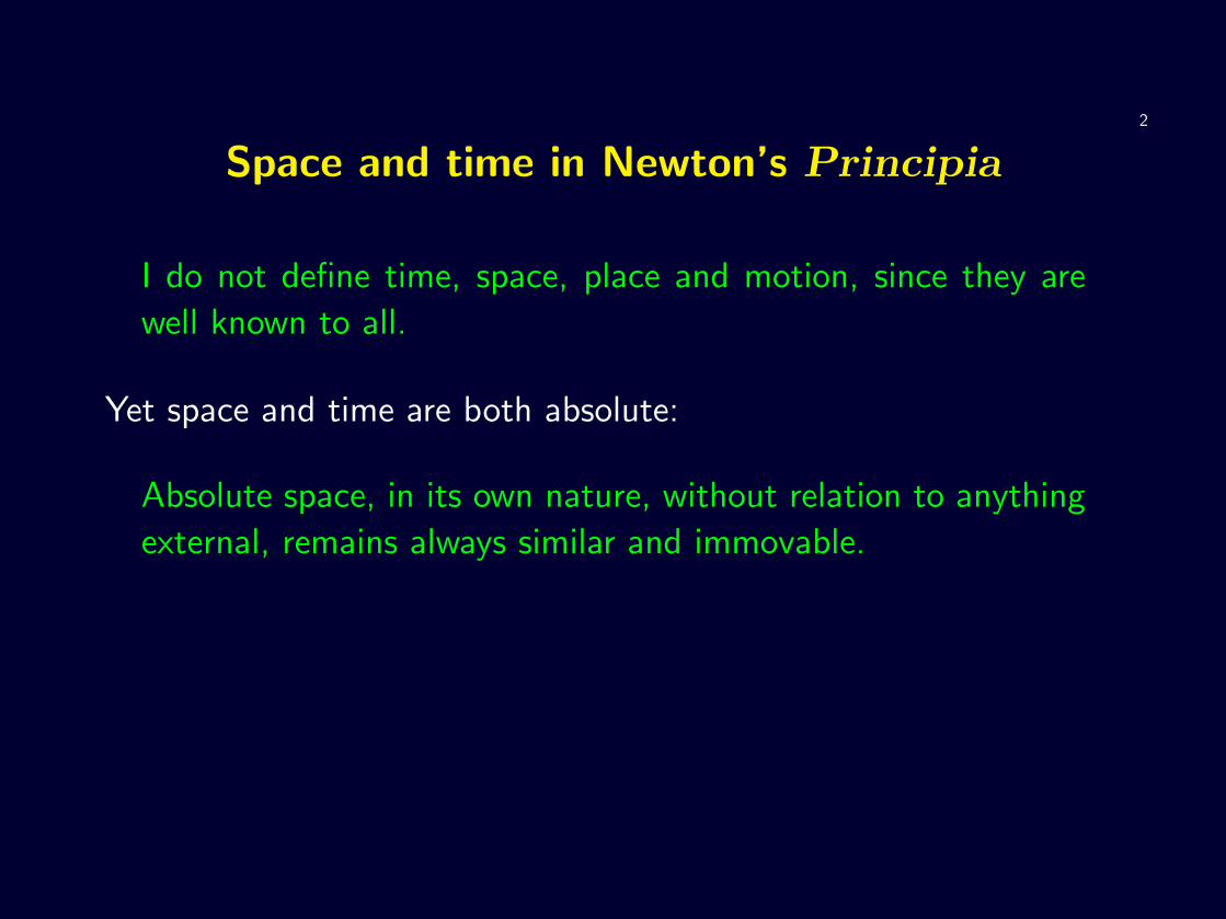
Space and time in Newton’s Principia
I do not define time, space, place and motion, since they are
well known to all.

2
Space and time in Newton’s Principia
I do not define time, space, place and motion, since they are
well known to all.
Yet space and time are both absolute
2
Space and time in Newton’s Principia
I do not define time, space, place and motion, since they are
well known to all.
Yet space and time are both absolute:
Absolute space, in its own nature, without relation to anything
external, remains always similar and immovable.
2
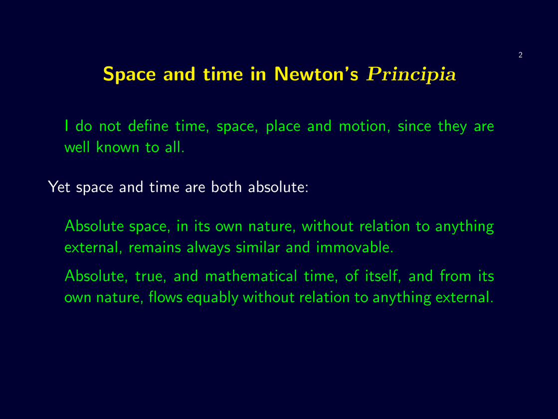
Space and time in Newton’s Principia
I do not define time, space, place and motion, since they are
well known to all.
Yet space and time are both absolute:
Absolute space, in its own nature, without relation to anything
external, remains always similar and immovable.
Absolute, true, and mathematical time, of itself, and from its
own nature, flows equably without relation to anything external.

2
Space and time in Newton’s Principia
I do not define time, space, place and motion, since they are
well known to all.
Yet space and time are both absolute:
Absolute space, in its own nature, without relation to anything
external, remains always similar and immovable.
Absolute, true, and mathematical time, of itself, and from its
own nature, flows equably without relation to anything external.
The Newtonian universe is thus R× R3.

3
Galilean relativity

3
Galilean relativity
• the motion of a point particle, say, is described by a path

3
Galilean relativity
• the motion of a point particle, say, is described by a path
x : [0, 1] → R3

3
Galilean relativity
• the motion of a point particle, say, is described by a path
x : [0, 1] → R3
subject to Newton’s equation

3
Galilean relativity
• the motion of a point particle, say, is described by a path
x : [0, 1] → R3
subject to Newton’s equation
x(t) = F (x(t))

3
Galilean relativity
• the motion of a point particle, say, is described by a path
x : [0, 1] → R3
subject to Newton’s equation
x(t) = F (x(t))
• if F = 0 particles move in straight lines

3
Galilean relativity
• the motion of a point particle, say, is described by a path
x : [0, 1] → R3
subject to Newton’s equation
x(t) = F (x(t))
• if F = 0 particles move in straight lines, and Newton’s equation

4
is invariant under Galilean transformations

4
is invariant under Galilean transformations
x 7→ x + tv

4
is invariant under Galilean transformations
x 7→ x + tv t 7→ t + a

4
is invariant under Galilean transformations
x 7→ x + tv t 7→ t + a
• velocities add

4
is invariant under Galilean transformations
x 7→ x + tv t 7→ t + a
• velocities add:
x(t) 7→ x(t) + v

4
is invariant under Galilean transformations
x 7→ x + tv t 7→ t + a
• velocities add:
x(t) 7→ x(t) + v
so there is no maximum velocity

4
is invariant under Galilean transformations
x 7→ x + tv t 7→ t + a
• velocities add:
x(t) 7→ x(t) + v
so there is no maximum velocity
• more generally, time intervals are invariant

4
is invariant under Galilean transformations
x 7→ x + tv t 7→ t + a
• velocities add:
x(t) 7→ x(t) + v
so there is no maximum velocity
• more generally, time intervals are invariant, and so are distances

4
is invariant under Galilean transformations
x 7→ x + tv t 7→ t + a
• velocities add:
x(t) 7→ x(t) + v
so there is no maximum velocity
• more generally, time intervals are invariant, and so are distances:
|x1 − tv − (x2 − tv)| = |x1 − x2|

5
Faraday’s field lines

5
Faraday’s field lines
• Michael Faraday envisioned novel objects moving in space

5
Faraday’s field lines
• Michael Faraday envisioned novel objects moving in space: space-
filling lines starting and ending on electric charges

5
Faraday’s field lines
• Michael Faraday envisioned novel objects moving in space: space-
filling lines starting and ending on electric charges

6
Maxwell equations

6
Maxwell equations
James Clerk Maxwell formulated Faraday’s electrical theory
mathematically

6
Maxwell equations
James Clerk Maxwell formulated Faraday’s electrical theory
mathematically:
curlE = −1c
∂B
∂t
curlB =1c
∂E
∂t

6
Maxwell equations
James Clerk Maxwell formulated Faraday’s electrical theory
mathematically:
curlE = −1c
∂B
∂t
curlB =1c
∂E
∂t
div E = 0
div B = 0

6
Maxwell equations
James Clerk Maxwell formulated Faraday’s electrical theory
mathematically:
curlE = −1c
∂B
∂t
curlB =1c
∂E
∂t
div E = 0
div B = 0
where E(x, t) and B(x, t) are the electric and magnetic fields,
respectively.

7
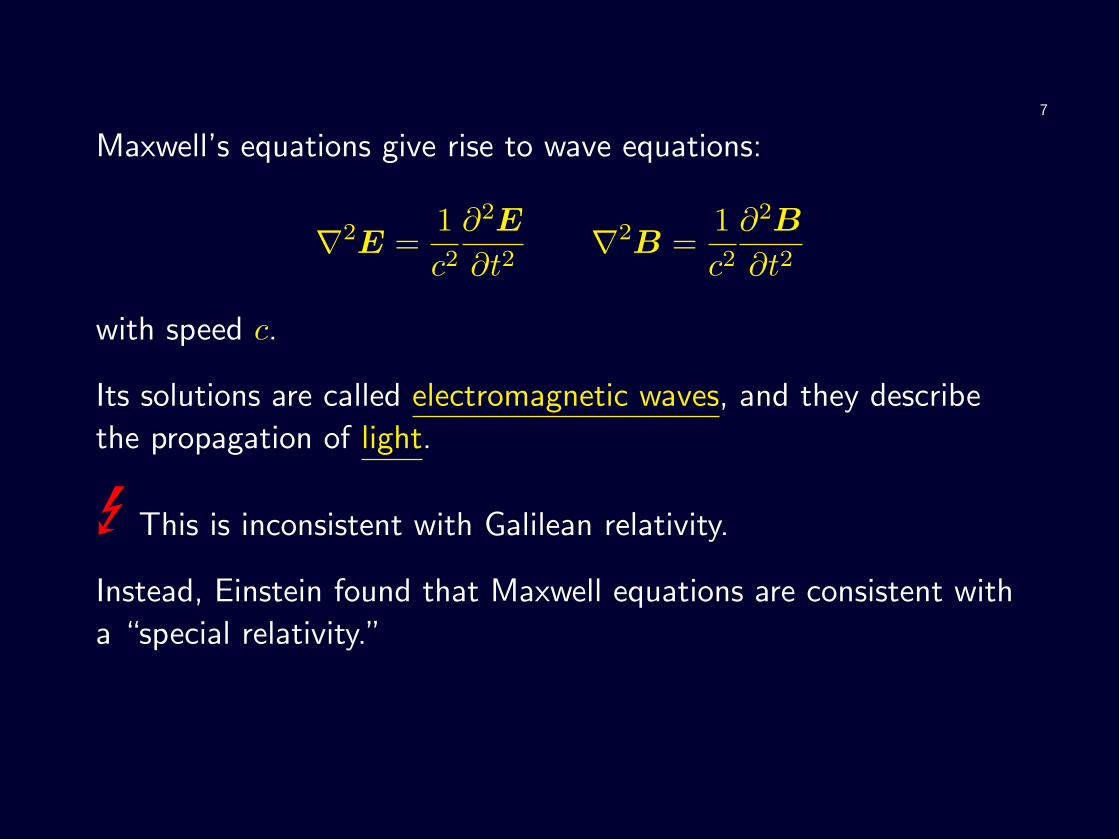
Maxwell’s equations give rise to wave equations:
∇2E =1c2
∂2E
∂t2

7
Maxwell’s equations give rise to wave equations:
∇2E =1c2
∂2E
∂t2∇2B =
1c2
∂2B
∂t2

7
Maxwell’s equations give rise to wave equations:
∇2E =1c2
∂2E
∂t2∇2B =
1c2
∂2B
∂t2
with speed c.

7
Maxwell’s equations give rise to wave equations:
∇2E =1c2
∂2E
∂t2∇2B =
1c2
∂2B
∂t2
with speed c.
Its solutions are called electromagnetic waves

7
Maxwell’s equations give rise to wave equations:
∇2E =1c2
∂2E
∂t2∇2B =
1c2
∂2B
∂t2
with speed c.
Its solutions are called electromagnetic waves, and they describe
the propagation of light.

7
Maxwell’s equations give rise to wave equations:
∇2E =1c2
∂2E
∂t2∇2B =
1c2
∂2B
∂t2
with speed c.
Its solutions are called electromagnetic waves, and they describe
the propagation of light.
E

7
Maxwell’s equations give rise to wave equations:
∇2E =1c2
∂2E
∂t2∇2B =
1c2
∂2B
∂t2
with speed c.
Its solutions are called electromagnetic waves, and they describe
the propagation of light.
E This is inconsistent with Galilean relativity.
7
Maxwell’s equations give rise to wave equations:
∇2E =1c2
∂2E
∂t2∇2B =
1c2
∂2B
∂t2
with speed c.
Its solutions are called electromagnetic waves, and they describe
the propagation of light.
E This is inconsistent with Galilean relativity.
Instead, Einstein found that Maxwell equations are consistent with
a “special relativity.”

8
Special Relativity

8
Special Relativity
In special relativity, the invariant quantity is the proper time

8
Special Relativity
In special relativity, the invariant quantity is the proper time
τ = |x1 − x2|2 − c2(t1 − t2)2

8
Special Relativity
In special relativity, the invariant quantity is the proper time
τ = |x1 − x2|2 − c2(t1 − t2)2
between two spacetime events (x1, t1) and (x2, t2)

8
Special Relativity
In special relativity, the invariant quantity is the proper time
τ = |x1 − x2|2 − c2(t1 − t2)2
between two spacetime events (x1, t1) and (x2, t2).
Z

8
Special Relativity
In special relativity, the invariant quantity is the proper time
τ = |x1 − x2|2 − c2(t1 − t2)2
between two spacetime events (x1, t1) and (x2, t2).
Zτ = 0 if and only if two events can be joined by a light ray.

8
Special Relativity
In special relativity, the invariant quantity is the proper time
τ = |x1 − x2|2 − c2(t1 − t2)2
between two spacetime events (x1, t1) and (x2, t2).
Zτ = 0 if and only if two events can be joined by a light ray.
Instead of Galilean transformations

8
Special Relativity
In special relativity, the invariant quantity is the proper time
τ = |x1 − x2|2 − c2(t1 − t2)2
between two spacetime events (x1, t1) and (x2, t2).
Zτ = 0 if and only if two events can be joined by a light ray.
Instead of Galilean transformations, we have
9
Lorentz transformations

9
Lorentz transformations:
x 7→ x + (γ − 1)(v · x)v
v2− γtv
t 7→ γ(t− v · xc2
)

9
Lorentz transformations:
x 7→ x + (γ − 1)(v · x)v
v2− γtv
t 7→ γ(t− v · xc2
)where γ =
1√1− ‖v‖2
c2

9
Lorentz transformations:
x 7→ x + (γ − 1)(v · x)v
v2− γtv
t 7→ γ(t− v · xc2
)where γ =
1√1− ‖v‖2
c2
More generally, a Lorentz transformation is a linear map
Λ : R4 → R4 preserving the Minkowski inner product

9
Lorentz transformations:
x 7→ x + (γ − 1)(v · x)v
v2− γtv
t 7→ γ(t− v · xc2
)where γ =
1√1− ‖v‖2
c2
More generally, a Lorentz transformation is a linear map
Λ : R4 → R4 preserving the Minkowski inner product:
〈(x1, t1), (x2, t2)〉 = x1 · x2 − c2t1t2

9
Lorentz transformations:
x 7→ x + (γ − 1)(v · x)v
v2− γtv
t 7→ γ(t− v · xc2
)where γ =
1√1− ‖v‖2
c2
More generally, a Lorentz transformation is a linear map
Λ : R4 → R4 preserving the Minkowski inner product:
〈(x1, t1), (x2, t2)〉 = x1 · x2 − c2t1t2
Z

9
Lorentz transformations:
x 7→ x + (γ − 1)(v · x)v
v2− γtv
t 7→ γ(t− v · xc2
)where γ =
1√1− ‖v‖2
c2
More generally, a Lorentz transformation is a linear map
Λ : R4 → R4 preserving the Minkowski inner product:
〈(x1, t1), (x2, t2)〉 = x1 · x2 − c2t1t2
Z 〈−,−〉 is indefinite

10
The electromagnetic universe is (R4, 〈−,−〉)

10
The electromagnetic universe is (R4, 〈−,−〉), which is called
Minkowski spacetime

10
The electromagnetic universe is (R4, 〈−,−〉), which is called
Minkowski spacetime, and is written E1,3

10
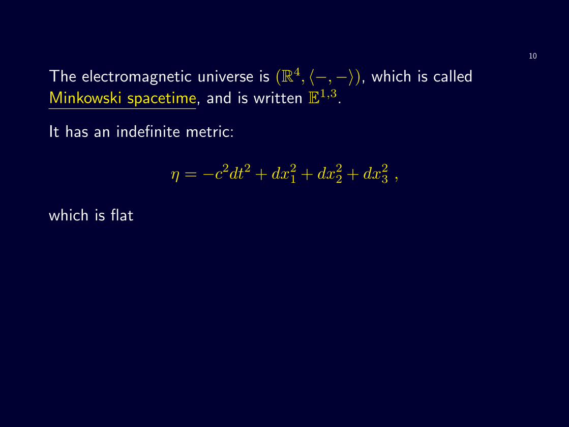
The electromagnetic universe is (R4, 〈−,−〉), which is called
Minkowski spacetime, and is written E1,3.
It has an indefinite metric

10
The electromagnetic universe is (R4, 〈−,−〉), which is called
Minkowski spacetime, and is written E1,3.
It has an indefinite metric:
η = −c2dt2 + dx21 + dx2
2 + dx23
10
The electromagnetic universe is (R4, 〈−,−〉), which is called
Minkowski spacetime, and is written E1,3.
It has an indefinite metric:
η = −c2dt2 + dx21 + dx2
2 + dx23 ,
which is flat
10
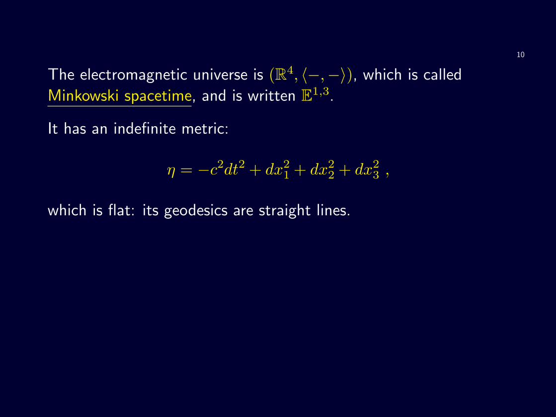
The electromagnetic universe is (R4, 〈−,−〉), which is called
Minkowski spacetime, and is written E1,3.
It has an indefinite metric:
η = −c2dt2 + dx21 + dx2
2 + dx23 ,
which is flat: its geodesics are straight lines.

11
General Relativity

11
General Relativity
• Galileo had discovered the equivalence principle

11
General Relativity
• Galileo had discovered the equivalence principle:
inertial mass = gravitational mass

11
General Relativity
• Galileo had discovered the equivalence principle:
inertial mass = gravitational mass
and Einstein geometrised it

11
General Relativity
• Galileo had discovered the equivalence principle:
inertial mass = gravitational mass
and Einstein geometrised it
• GR mantra

11
General Relativity
• Galileo had discovered the equivalence principle:
inertial mass = gravitational mass
and Einstein geometrised it
• GR mantra:
Spacetime tells matter how to move

11
General Relativity
• Galileo had discovered the equivalence principle:
inertial mass = gravitational mass
and Einstein geometrised it
• GR mantra:
Spacetime tells matter how to move, and matter tells
spacetime how to curve.

12
• Mathematically
12
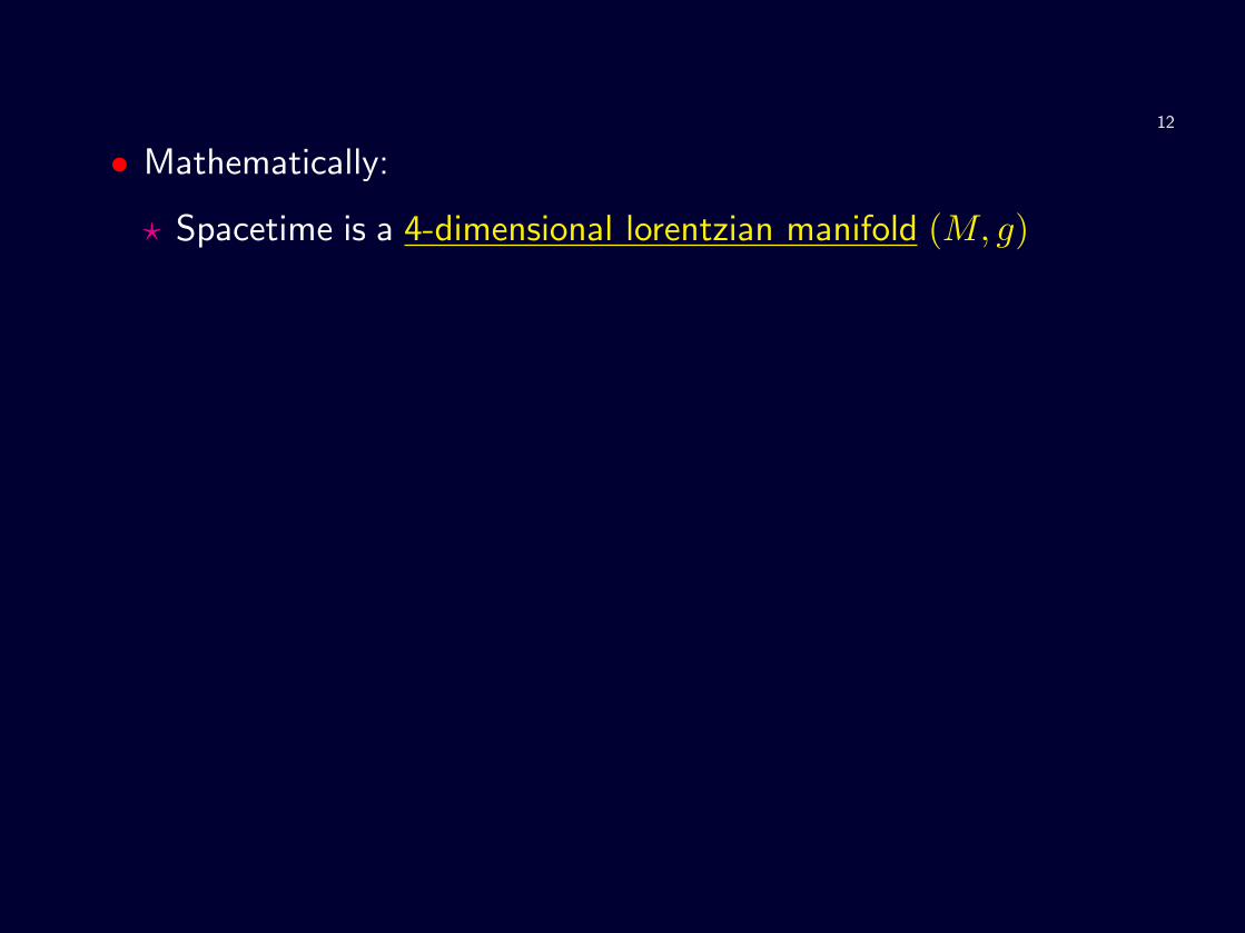
• Mathematically:
? Spacetime is a 4-dimensional lorentzian manifold (M, g)

12
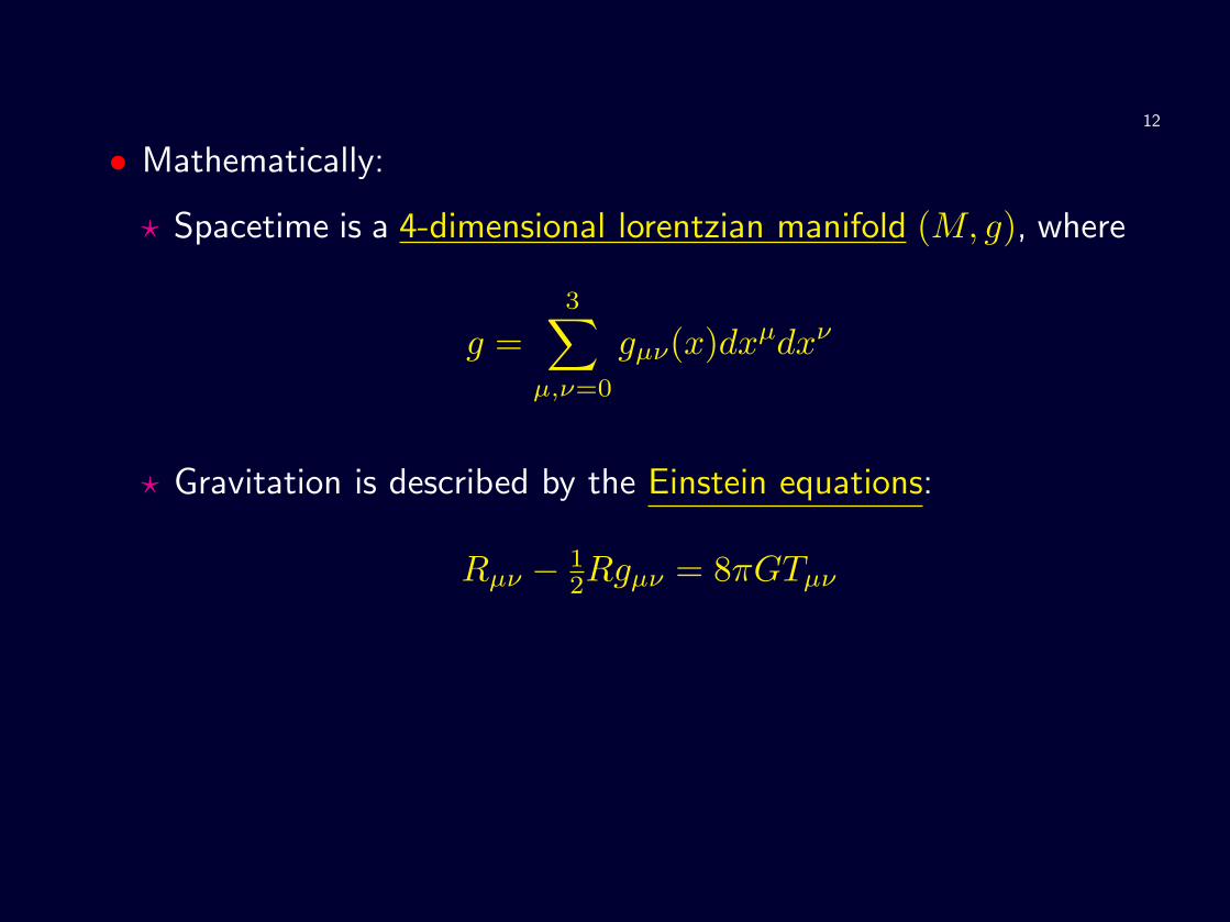
• Mathematically:
? Spacetime is a 4-dimensional lorentzian manifold (M, g), where
g =3∑
µ,ν=0
gµν(x)dxµdxν

12
• Mathematically:
? Spacetime is a 4-dimensional lorentzian manifold (M, g), where
g =3∑
µ,ν=0
gµν(x)dxµdxν
? Gravitation is described by the Einstein equations
12
• Mathematically:
? Spacetime is a 4-dimensional lorentzian manifold (M, g), where
g =3∑
µ,ν=0
gµν(x)dxµdxν
? Gravitation is described by the Einstein equations:
Rµν − 12Rgµν = 8πGTµν

12
• Mathematically:
? Spacetime is a 4-dimensional lorentzian manifold (M, g), where
g =3∑
µ,ν=0
gµν(x)dxµdxν
? Gravitation is described by the Einstein equations:
Rµν − 12Rgµν = 8πGTµν
Which spacetime (M, g) describes our universe?
13
Empirical basis for FLRW cosmology

13
Empirical basis for FLRW cosmology
• Hubble (1920s)
13
Empirical basis for FLRW cosmology
• Hubble (1920s)
? uniform redshift of spectral lines in all directions
13
Empirical basis for FLRW cosmology
• Hubble (1920s)
? uniform redshift of spectral lines in all directions and growing
with distance

13
Empirical basis for FLRW cosmology
• Hubble (1920s)
? uniform redshift of spectral lines in all directions and growing
with distance
? space between stars is expanding isotropically

13
Empirical basis for FLRW cosmology
• Hubble (1920s)
? uniform redshift of spectral lines in all directions and growing
with distance
? space between stars is expanding isotropically
? “principle of mediocrity” =⇒ homogeneity

13
Empirical basis for FLRW cosmology
• Hubble (1920s)
? uniform redshift of spectral lines in all directions and growing
with distance
? space between stars is expanding isotropically
? “principle of mediocrity” =⇒ homogeneity
• Penzias and Wilson (1965)

13
Empirical basis for FLRW cosmology
• Hubble (1920s)
? uniform redshift of spectral lines in all directions and growing
with distance
? space between stars is expanding isotropically
? “principle of mediocrity” =⇒ homogeneity
• Penzias and Wilson (1965):
? discovered Cosmic Microwave Background

13
Empirical basis for FLRW cosmology
• Hubble (1920s)
? uniform redshift of spectral lines in all directions and growing
with distance
? space between stars is expanding isotropically
? “principle of mediocrity” =⇒ homogeneity
• Penzias and Wilson (1965):
? discovered Cosmic Microwave Background
? confirms homogeneity and isotropy at large scales

14
At large scales, our universe is described by R× Σ

14
At large scales, our universe is described by R× Σ, with R the
cosmological time

14
At large scales, our universe is described by R× Σ, with R the
cosmological time, and Σ a three-dimensional manifold of constant
curvature

14
At large scales, our universe is described by R× Σ, with R the
cosmological time, and Σ a three-dimensional manifold of constant
curvature: our spatial universe.

14
At large scales, our universe is described by R× Σ, with R the
cosmological time, and Σ a three-dimensional manifold of constant
curvature: our spatial universe.
The geometry is described by a
Friedmann–Lemaıtre–Robertson–Walker metric

14
At large scales, our universe is described by R× Σ, with R the
cosmological time, and Σ a three-dimensional manifold of constant
curvature: our spatial universe.
The geometry is described by a
Friedmann–Lemaıtre–Robertson–Walker metric:
−dt2 + a(t)2h
where h is the metric on Σ.

14
At large scales, our universe is described by R× Σ, with R the
cosmological time, and Σ a three-dimensional manifold of constant
curvature: our spatial universe.
The geometry is described by a
Friedmann–Lemaıtre–Robertson–Walker metric:
−dt2 + a(t)2h
where h is the metric on Σ.
a(t) is determined from the Einstein equations

14
At large scales, our universe is described by R× Σ, with R the
cosmological time, and Σ a three-dimensional manifold of constant
curvature: our spatial universe.
The geometry is described by a
Friedmann–Lemaıtre–Robertson–Walker metric:
−dt2 + a(t)2h
where h is the metric on Σ.
a(t) is determined from the Einstein equations, which depend on
the “matter” content of the universe

14
At large scales, our universe is described by R× Σ, with R the
cosmological time, and Σ a three-dimensional manifold of constant
curvature: our spatial universe.
The geometry is described by a
Friedmann–Lemaıtre–Robertson–Walker metric:
−dt2 + a(t)2h
where h is the metric on Σ.
a(t) is determined from the Einstein equations, which depend on
the “matter” content of the universe, currently

15

16
The geometry and topology of the spatial universe
16
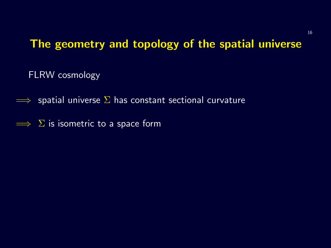
The geometry and topology of the spatial universe
FLRW cosmology

16
The geometry and topology of the spatial universe
FLRW cosmology
=⇒ spatial universe Σ has constant sectional curvature
16
The geometry and topology of the spatial universe
FLRW cosmology
=⇒ spatial universe Σ has constant sectional curvature
=⇒ Σ is isometric to a space form

16
The geometry and topology of the spatial universe
FLRW cosmology
=⇒ spatial universe Σ has constant sectional curvature
=⇒ Σ is isometric to a space form
=⇒ Σ is isometric to Σ/Γ

16
The geometry and topology of the spatial universe
FLRW cosmology
=⇒ spatial universe Σ has constant sectional curvature
=⇒ Σ is isometric to a space form
=⇒ Σ is isometric to Σ/Γ, where Σ is a simply-connected three-
dimensional space form

16
The geometry and topology of the spatial universe
FLRW cosmology
=⇒ spatial universe Σ has constant sectional curvature
=⇒ Σ is isometric to a space form
=⇒ Σ is isometric to Σ/Γ, where Σ is a simply-connected three-
dimensional space form, and Γ is a discrete subgroup of the
isometries of Σ

17
The metric h on Σ takes the form

17
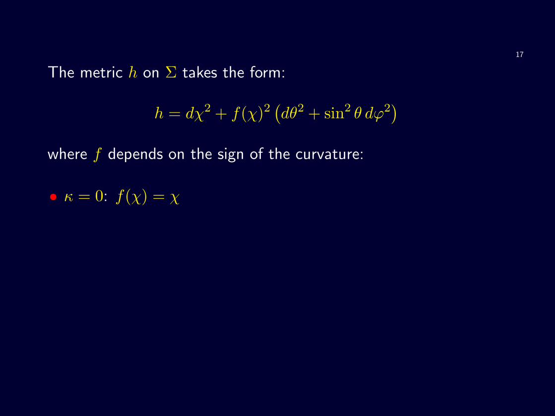
The metric h on Σ takes the form:
h = dχ2 + f(χ)2(dθ2 + sin2 θ dϕ2
)

17
The metric h on Σ takes the form:
h = dχ2 + f(χ)2(dθ2 + sin2 θ dϕ2
)where f depends on the sign of the curvature

17
The metric h on Σ takes the form:
h = dχ2 + f(χ)2(dθ2 + sin2 θ dϕ2
)where f depends on the sign of the curvature:
• κ = 0
17
The metric h on Σ takes the form:
h = dχ2 + f(χ)2(dθ2 + sin2 θ dϕ2
)where f depends on the sign of the curvature:
• κ = 0: f(χ) = χ

17
The metric h on Σ takes the form:
h = dχ2 + f(χ)2(dθ2 + sin2 θ dϕ2
)where f depends on the sign of the curvature:
• κ = 0: f(χ) = χ
• κ = 1

17
The metric h on Σ takes the form:
h = dχ2 + f(χ)2(dθ2 + sin2 θ dϕ2
)where f depends on the sign of the curvature:
• κ = 0: f(χ) = χ
• κ = 1: f(χ) = sin χ

17
The metric h on Σ takes the form:
h = dχ2 + f(χ)2(dθ2 + sin2 θ dϕ2
)where f depends on the sign of the curvature:
• κ = 0: f(χ) = χ
• κ = 1: f(χ) = sin χ
• κ = −1

17
The metric h on Σ takes the form:
h = dχ2 + f(χ)2(dθ2 + sin2 θ dϕ2
)where f depends on the sign of the curvature:
• κ = 0: f(χ) = χ
• κ = 1: f(χ) = sin χ
• κ = −1: f(χ) = sinhχ

18
• κ = 0

18
• κ = 0 (flat)

18
• κ = 0 (flat): Σ = E3

18
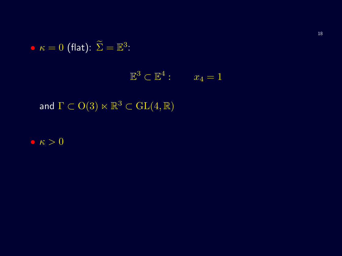
• κ = 0 (flat): Σ = E3:
E3 ⊂ E4

18
• κ = 0 (flat): Σ = E3:
E3 ⊂ E4 : x4 = 1

18
• κ = 0 (flat): Σ = E3:
E3 ⊂ E4 : x4 = 1
and Γ ⊂ O(3) n R3 ⊂ GL(4, R)
18
• κ = 0 (flat): Σ = E3:
E3 ⊂ E4 : x4 = 1
and Γ ⊂ O(3) n R3 ⊂ GL(4, R)
• κ > 0

18
• κ = 0 (flat): Σ = E3:
E3 ⊂ E4 : x4 = 1
and Γ ⊂ O(3) n R3 ⊂ GL(4, R)
• κ > 0 (spherical)

18
• κ = 0 (flat): Σ = E3:
E3 ⊂ E4 : x4 = 1
and Γ ⊂ O(3) n R3 ⊂ GL(4, R)
• κ > 0 (spherical): Σ = S3

18
• κ = 0 (flat): Σ = E3:
E3 ⊂ E4 : x4 = 1
and Γ ⊂ O(3) n R3 ⊂ GL(4, R)
• κ > 0 (spherical): Σ = S3:
S3 ⊂ E4

18
• κ = 0 (flat): Σ = E3:
E3 ⊂ E4 : x4 = 1
and Γ ⊂ O(3) n R3 ⊂ GL(4, R)
• κ > 0 (spherical): Σ = S3:
S3 ⊂ E4 : x21 + x2
2 + x23 + x2
4 =1κ2

18
• κ = 0 (flat): Σ = E3:
E3 ⊂ E4 : x4 = 1
and Γ ⊂ O(3) n R3 ⊂ GL(4, R)
• κ > 0 (spherical): Σ = S3:
S3 ⊂ E4 : x21 + x2
2 + x23 + x2
4 =1κ2
and Γ ⊂ O(4)

19
• κ < 0

19
• κ < 0 (hyperbolic)

19
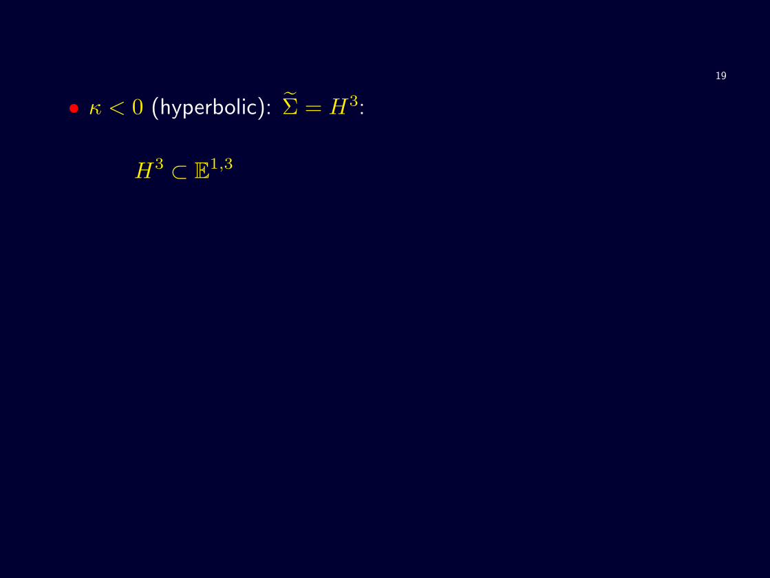
• κ < 0 (hyperbolic): Σ = H3
19
• κ < 0 (hyperbolic): Σ = H3:
H3 ⊂ E1,3

19
• κ < 0 (hyperbolic): Σ = H3:
H3 ⊂ E1,3 : −x20 + x2
1 + x22 + x2
3 =−1κ2

19
• κ < 0 (hyperbolic): Σ = H3:
H3 ⊂ E1,3 : −x20 + x2
1 + x22 + x2
3 =−1κ2
x0 > 0

19
• κ < 0 (hyperbolic): Σ = H3:
H3 ⊂ E1,3 : −x20 + x2
1 + x22 + x2
3 =−1κ2
x0 > 0
and Γ ⊂ O(1, 3)

19
• κ < 0 (hyperbolic): Σ = H3:
H3 ⊂ E1,3 : −x20 + x2
1 + x22 + x2
3 =−1κ2
x0 > 0
and Γ ⊂ O(1, 3)
Spherical and hyperbolic spaceforms are rigid

19
• κ < 0 (hyperbolic): Σ = H3:
H3 ⊂ E1,3 : −x20 + x2
1 + x22 + x2
3 =−1κ2
x0 > 0
and Γ ⊂ O(1, 3)
Spherical and hyperbolic spaceforms are rigid: their topology
determines their geometry!

19
• κ < 0 (hyperbolic): Σ = H3:
H3 ⊂ E1,3 : −x20 + x2
1 + x22 + x2
3 =−1κ2
x0 > 0
and Γ ⊂ O(1, 3)
Spherical and hyperbolic spaceforms are rigid: their topology
determines their geometry! (e.g., Mostow rigidity)

19
• κ < 0 (hyperbolic): Σ = H3:
H3 ⊂ E1,3 : −x20 + x2
1 + x22 + x2
3 =−1κ2
x0 > 0
and Γ ⊂ O(1, 3)
Spherical and hyperbolic spaceforms are rigid: their topology
determines their geometry! (e.g., Mostow rigidity)
Big question

19
• κ < 0 (hyperbolic): Σ = H3:
H3 ⊂ E1,3 : −x20 + x2
1 + x22 + x2
3 =−1κ2
x0 > 0
and Γ ⊂ O(1, 3)
Spherical and hyperbolic spaceforms are rigid: their topology
determines their geometry! (e.g., Mostow rigidity)
Big question:
Which topology do we inhabit?
20
Large scale anisotropy in the CMB

20
Large scale anisotropy in the CMB
The COsmic Background Explorer showed large scale anisotropy

20
Large scale anisotropy in the CMB
The COsmic Background Explorer showed large scale anisotropy

21
The Wilkinson Microwave Anisotropy Probe refined the data

21
The Wilkinson Microwave Anisotropy Probe refined the data:

22
Physics of the CMB

22
Physics of the CMB
• CMB results from photons produced in the early universe

22
Physics of the CMB
• CMB results from photons produced in the early universe
• WMAP data is a snapshot of the “surface of last scatter”

22
Physics of the CMB
• CMB results from photons produced in the early universe
• WMAP data is a snapshot of the “surface of last scatter”
• CMB is measured in temperature

22
Physics of the CMB
• CMB results from photons produced in the early universe
• WMAP data is a snapshot of the “surface of last scatter”
• CMB is measured in temperature: / 3◦K

22
Physics of the CMB
• CMB results from photons produced in the early universe
• WMAP data is a snapshot of the “surface of last scatter”
• CMB is measured in temperature: / 3◦K
• anisotropy is measured as “temperature fluctuations”

22
Physics of the CMB
• CMB results from photons produced in the early universe
• WMAP data is a snapshot of the “surface of last scatter”
• CMB is measured in temperature: / 3◦K
• anisotropy is measured as “temperature fluctuations”, and is due
to density fluctuations in the early universe

23
We introduce a “scalar perturbation” to the FLRW metric

23
We introduce a “scalar perturbation” to the FLRW metric:
−(1 + 2Φ)dt2 + a(t)2(1− 2Φ)h

23
We introduce a “scalar perturbation” to the FLRW metric:
−(1 + 2Φ)dt2 + a(t)2(1− 2Φ)h
in the form of a “gravitational potential”

23
We introduce a “scalar perturbation” to the FLRW metric:
−(1 + 2Φ)dt2 + a(t)2(1− 2Φ)h
in the form of a “gravitational potential” Φ : R× Σ → R.
23
We introduce a “scalar perturbation” to the FLRW metric:
−(1 + 2Φ)dt2 + a(t)2(1− 2Φ)h
in the form of a “gravitational potential” Φ : R× Σ → R.
The time evolution of Φ is fixed by the Einstein equations
23
We introduce a “scalar perturbation” to the FLRW metric:
−(1 + 2Φ)dt2 + a(t)2(1− 2Φ)h
in the form of a “gravitational potential” Φ : R× Σ → R.
The time evolution of Φ is fixed by the Einstein equations, whence
it is determined by its “initial value” Φ0 : Σ → R.

23
We introduce a “scalar perturbation” to the FLRW metric:
−(1 + 2Φ)dt2 + a(t)2(1− 2Φ)h
in the form of a “gravitational potential” Φ : R× Σ → R.
The time evolution of Φ is fixed by the Einstein equations, whence
it is determined by its “initial value” Φ0 : Σ → R.
The “Sachs–Wolfe effect” relates the temperature fluctuations in
the CMB to Φ0.

24
Strategy

24
Strategy: Try to work out Φ0 from WMAP data

24
Strategy: Try to work out Φ0 from WMAP data, and hence the
geometry of Σ.

24
Strategy: Try to work out Φ0 from WMAP data, and hence the
geometry of Σ.
• WMAP data defines Ψ : S2 → R

24
Strategy: Try to work out Φ0 from WMAP data, and hence the
geometry of Σ.
• WMAP data defines Ψ : S2 → R, which we expand in spherical
harmonics

24
Strategy: Try to work out Φ0 from WMAP data, and hence the
geometry of Σ.
• WMAP data defines Ψ : S2 → R, which we expand in spherical
harmonics
• gravitational potential Φ0 : Σ → R

24
Strategy: Try to work out Φ0 from WMAP data, and hence the
geometry of Σ.
• WMAP data defines Ψ : S2 → R, which we expand in spherical
harmonics
• gravitational potential Φ0 : Σ → R, which we can also expand in
harmonics on Σ

24
Strategy: Try to work out Φ0 from WMAP data, and hence the
geometry of Σ.
• WMAP data defines Ψ : S2 → R, which we expand in spherical
harmonics
• gravitational potential Φ0 : Σ → R, which we can also expand in
harmonics on Σ
• lowest lying modes in expansion of Φ0 carry information about the
topology of Σ

24
Strategy: Try to work out Φ0 from WMAP data, and hence the
geometry of Σ.
• WMAP data defines Ψ : S2 → R, which we expand in spherical
harmonics
• gravitational potential Φ0 : Σ → R, which we can also expand in
harmonics on Σ
• lowest lying modes in expansion of Φ0 carry information about the
topology of Σ, and feed into the lowest lying modes in expansion
of Ψ
There is a related mathematical problem...

25
Can we hear the shape of the universe?

25
Can we hear the shape of the universe?
We can determine the length of a string by hearing it vibrate

25
Can we hear the shape of the universe?
We can determine the length of a string by hearing it vibrate.
Mark Kac (1966)

25
Can we hear the shape of the universe?
We can determine the length of a string by hearing it vibrate.
Mark Kac (1966): Can we hear the shape of a drum?

25
Can we hear the shape of the universe?
We can determine the length of a string by hearing it vibrate.
Mark Kac (1966): Can we hear the shape of a drum?
Mathematically, given a riemannian manifold (M, g), consider the
Laplacian operator ∆ acting on functions

25
Can we hear the shape of the universe?
We can determine the length of a string by hearing it vibrate.
Mark Kac (1966): Can we hear the shape of a drum?
Mathematically, given a riemannian manifold (M, g), consider the
Laplacian operator ∆ acting on functions:
∆f(x) =∑i,j
gij(x)∇i∇jf(x)

25
Can we hear the shape of the universe?
We can determine the length of a string by hearing it vibrate.
Mark Kac (1966): Can we hear the shape of a drum?
Mathematically, given a riemannian manifold (M, g), consider the
Laplacian operator ∆ acting on functions:
∆f(x) =∑i,j
gij(x)∇i∇jf(x)
with ∇ the riemannian connection.

26
The eigenvalues of ∆ define the spectrum of (M, g)

26
The eigenvalues of ∆ define the spectrum of (M, g).
Kac’s question is

26
The eigenvalues of ∆ define the spectrum of (M, g).
Kac’s question is:
Are isospectral 2-manifolds isometric?

26
The eigenvalues of ∆ define the spectrum of (M, g).
Kac’s question is:
Are isospectral 2-manifolds isometric?
The answer is known to be false in general

26
The eigenvalues of ∆ define the spectrum of (M, g).
Kac’s question is:
Are isospectral 2-manifolds isometric?
The answer is known to be false in general:
Milnor (1964)

26
The eigenvalues of ∆ define the spectrum of (M, g).
Kac’s question is:
Are isospectral 2-manifolds isometric?
The answer is known to be false in general:
Milnor (1964): R16/Λ1 and R16/Λ2 are isospectral but not
isometric.
26
The eigenvalues of ∆ define the spectrum of (M, g).
Kac’s question is:
Are isospectral 2-manifolds isometric?
The answer is known to be false in general:
Milnor (1964): R16/Λ1 and R16/Λ2 are isospectral but not
isometric.
More recent counterexamples

26
The eigenvalues of ∆ define the spectrum of (M, g).
Kac’s question is:
Are isospectral 2-manifolds isometric?
The answer is known to be false in general:
Milnor (1964): R16/Λ1 and R16/Λ2 are isospectral but not
isometric.
More recent counterexamples: planar domains.

26
The eigenvalues of ∆ define the spectrum of (M, g).
Kac’s question is:
Are isospectral 2-manifolds isometric?
The answer is known to be false in general:
Milnor (1964): R16/Λ1 and R16/Λ2 are isospectral but not
isometric.
More recent counterexamples: planar domains.
But it is true for three-dimensional space-forms!

27
Spherical harmonics
27
Spherical harmonics
• F : R3 → R: a homogeneous polynomial of degree `

27
Spherical harmonics
• F : R3 → R: a homogeneous polynomial of degree `
• F = r`f

27
Spherical harmonics
• F : R3 → R: a homogeneous polynomial of degree `
• F = r`f , where f : S2 → R

27
Spherical harmonics
• F : R3 → R: a homogeneous polynomial of degree `
• F = r`f , where f : S2 → R
• F is harmonic ⇐⇒ ∆f = −`(` + 1)f on S2

27
Spherical harmonics
• F : R3 → R: a homogeneous polynomial of degree `
• F = r`f , where f : S2 → R
• F is harmonic ⇐⇒ ∆f = −`(` + 1)f on S2
• all eigenfunctions of ∆ are obtained in this way

27
Spherical harmonics
• F : R3 → R: a homogeneous polynomial of degree `
• F = r`f , where f : S2 → R
• F is harmonic ⇐⇒ ∆f = −`(` + 1)f on S2
• all eigenfunctions of ∆ are obtained in this way
• the eigenspace V` with eigenvalue −`(`+1) has dimension 2`+1

27
Spherical harmonics
• F : R3 → R: a homogeneous polynomial of degree `
• F = r`f , where f : S2 → R
• F is harmonic ⇐⇒ ∆f = −`(` + 1)f on S2
• all eigenfunctions of ∆ are obtained in this way
• the eigenspace V` with eigenvalue −`(`+1) has dimension 2`+1
• V` is an irreducible representation of SO(3)

28
• spherical harmonics Y` m

28
• spherical harmonics Y` m, m = −`, ..., `

28
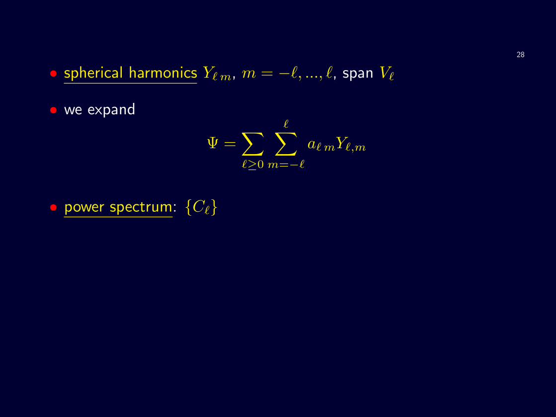
• spherical harmonics Y` m, m = −`, ..., `, span V`

28
• spherical harmonics Y` m, m = −`, ..., `, span V`
• we expand
Ψ =∑`≥0
∑m=−`
a` mY`,m
28
• spherical harmonics Y` m, m = −`, ..., `, span V`
• we expand
Ψ =∑`≥0
∑m=−`
a` mY`,m
• power spectrum: {C`}

28
• spherical harmonics Y` m, m = −`, ..., `, span V`
• we expand
Ψ =∑`≥0
∑m=−`
a` mY`,m
• power spectrum: {C`}, where
C` =∑
m=−`
|a` m|2

28
• spherical harmonics Y` m, m = −`, ..., `, span V`
• we expand
Ψ =∑`≥0
∑m=−`
a` mY`,m
• power spectrum: {C`}, where
C` =∑
m=−`
|a` m|2
• WMAP data gives {C`} up to ` ∼ 100

29
A spherical universe

29
A spherical universe
Consider a spherical universe Σ = S3/Γ

29
A spherical universe
Consider a spherical universe Σ = S3/Γ.
• functions on S3/Γ are Γ-invariant functions on S3

29
A spherical universe
Consider a spherical universe Σ = S3/Γ.
• functions on S3/Γ are Γ-invariant functions on S3
• S3 and S3/Γ are locally isometric

29
A spherical universe
Consider a spherical universe Σ = S3/Γ.
• functions on S3/Γ are Γ-invariant functions on S3
• S3 and S3/Γ are locally isometric
=⇒ laplacians on S3 and on S3/Γ agree
29
A spherical universe
Consider a spherical universe Σ = S3/Γ.
• functions on S3/Γ are Γ-invariant functions on S3
• S3 and S3/Γ are locally isometric
=⇒ laplacians on S3 and on S3/Γ agree
• eigenfunctions on S3/Γ are Γ-invariant spherical harmonics
30
Spherical harmonics on S3

30
Spherical harmonics on S3
• F : R4 → R: a homogeneous polynomial of degree k

30
Spherical harmonics on S3
• F : R4 → R: a homogeneous polynomial of degree k
• F = rkf

30
Spherical harmonics on S3
• F : R4 → R: a homogeneous polynomial of degree k
• F = rkf , where f : S3 → R

30
Spherical harmonics on S3
• F : R4 → R: a homogeneous polynomial of degree k
• F = rkf , where f : S3 → R
• F is harmonic ⇐⇒ ∆f = −k(k + 2)f on S3

30
Spherical harmonics on S3
• F : R4 → R: a homogeneous polynomial of degree k
• F = rkf , where f : S3 → R
• F is harmonic ⇐⇒ ∆f = −k(k + 2)f on S3
• all eigenfunctions of ∆ are obtained in this way

30
Spherical harmonics on S3
• F : R4 → R: a homogeneous polynomial of degree k
• F = rkf , where f : S3 → R
• F is harmonic ⇐⇒ ∆f = −k(k + 2)f on S3
• all eigenfunctions of ∆ are obtained in this way
• the eigenspace Vk with eigenvalue −k(k + 2) has dimension
(k + 1)2

30
Spherical harmonics on S3
• F : R4 → R: a homogeneous polynomial of degree k
• F = rkf , where f : S3 → R
• F is harmonic ⇐⇒ ∆f = −k(k + 2)f on S3
• all eigenfunctions of ∆ are obtained in this way
• the eigenspace Vk with eigenvalue −k(k + 2) has dimension
(k + 1)2
• Vk is an irreducible representation of SO(4)

31
Subgroups Γ ⊂ SO(4)

31
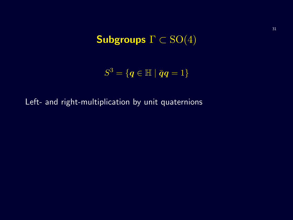
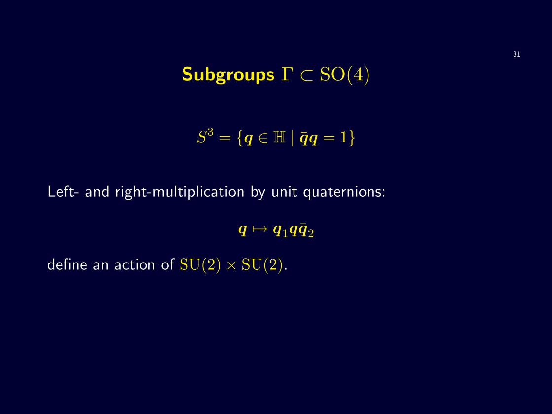
Subgroups Γ ⊂ SO(4)
S3 = {q ∈ H | qq = 1}
31
Subgroups Γ ⊂ SO(4)
S3 = {q ∈ H | qq = 1}
Left- and right-multiplication by unit quaternions

31
Subgroups Γ ⊂ SO(4)
S3 = {q ∈ H | qq = 1}
Left- and right-multiplication by unit quaternions:
q 7→ q1qq2
31
Subgroups Γ ⊂ SO(4)
S3 = {q ∈ H | qq = 1}
Left- and right-multiplication by unit quaternions:
q 7→ q1qq2
define an action of SU(2)× SU(2).

31
Subgroups Γ ⊂ SO(4)
S3 = {q ∈ H | qq = 1}
Left- and right-multiplication by unit quaternions:
q 7→ q1qq2
define an action of SU(2)× SU(2).
The element (−1,−1) acts trivially

31
Subgroups Γ ⊂ SO(4)
S3 = {q ∈ H | qq = 1}
Left- and right-multiplication by unit quaternions:
q 7→ q1qq2
define an action of SU(2)× SU(2).
The element (−1,−1) acts trivially, so we have an action of
SO(4) = (SU(2)× SU(2)) /Z2

32
Let Γ ⊂ SO(4) be a finite subgroup
32
Let Γ ⊂ SO(4) be a finite subgroup.
Three types

32
Let Γ ⊂ SO(4) be a finite subgroup.
Three types:
• left-acting: q 7→ γq, γ ∈ Γ

32
Let Γ ⊂ SO(4) be a finite subgroup.
Three types:
• left-acting: q 7→ γq, γ ∈ Γ
• right-acting: q 7→ qγ, γ ∈ Γ

32
Let Γ ⊂ SO(4) be a finite subgroup.
Three types:
• left-acting: q 7→ γq, γ ∈ Γ
• right-acting: q 7→ qγ, γ ∈ Γ
• doubly-acting

32
Let Γ ⊂ SO(4) be a finite subgroup.
Three types:
• left-acting: q 7→ γq, γ ∈ Γ
• right-acting: q 7→ qγ, γ ∈ Γ
• doubly-acting
For the first two types

32
Let Γ ⊂ SO(4) be a finite subgroup.
Three types:
• left-acting: q 7→ γq, γ ∈ Γ
• right-acting: q 7→ qγ, γ ∈ Γ
• doubly-acting
For the first two types: Γ ⊂ SU(2).

33
Finite subgroups Γ ⊂ SU(2)

33
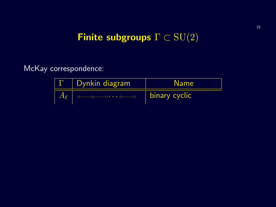
Finite subgroups Γ ⊂ SU(2)
McKay correspondence

33
Finite subgroups Γ ⊂ SU(2)
McKay correspondence:
Γ Dynkin diagram Name
33
Finite subgroups Γ ⊂ SU(2)
McKay correspondence:
Γ Dynkin diagram Name
A` e e e e e· · · binary cyclic

33
Finite subgroups Γ ⊂ SU(2)
McKay correspondence:
Γ Dynkin diagram Name
A` e e e e e· · · binary cyclic
D` e e e e e· · ·
ebinary dihedral

33
Finite subgroups Γ ⊂ SU(2)
McKay correspondence:
Γ Dynkin diagram Name
A` e e e e e· · · binary cyclic
D` e e e e e· · ·
ebinary dihedral
E6 e e e e ee
binary tetrahedral

33
Finite subgroups Γ ⊂ SU(2)
McKay correspondence:
Γ Dynkin diagram Name
A` e e e e e· · · binary cyclic
D` e e e e e· · ·
ebinary dihedral
E6 e e e e ee
binary tetrahedral
E7 e e e e e ee
binary octahedral

33
Finite subgroups Γ ⊂ SU(2)
McKay correspondence:
Γ Dynkin diagram Name
A` e e e e e· · · binary cyclic
D` e e e e e· · ·
ebinary dihedral
E6 e e e e ee
binary tetrahedral
E7 e e e e e ee
binary octahedral
E8 e e e e e e ee
binary dodecahedral

34
And the answer is...

34
And the answer is...
Luminet, Weeks, Riazuelo, Lehoucq and Uzan (2003)

34
And the answer is...
Luminet, Weeks, Riazuelo, Lehoucq and Uzan (2003) found that
the first year WMAP data suggests

34
And the answer is...
Luminet, Weeks, Riazuelo, Lehoucq and Uzan (2003) found that
the first year WMAP data suggests:
Σ ∼=

34
And the answer is...
Luminet, Weeks, Riazuelo, Lehoucq and Uzan (2003) found that
the first year WMAP data suggests:
Σ ∼= S3/

34
And the answer is...
Luminet, Weeks, Riazuelo, Lehoucq and Uzan (2003) found that
the first year WMAP data suggests:
Σ ∼= S3/E8 (!)

34
And the answer is...
Luminet, Weeks, Riazuelo, Lehoucq and Uzan (2003) found that
the first year WMAP data suggests:
Σ ∼= S3/E8 (!)
• the universe is finite!

34
And the answer is...
Luminet, Weeks, Riazuelo, Lehoucq and Uzan (2003) found that
the first year WMAP data suggests:
Σ ∼= S3/E8 (!)
• the universe is finite!
• π1(Σ) ∼= E8

34
And the answer is...
Luminet, Weeks, Riazuelo, Lehoucq and Uzan (2003) found that
the first year WMAP data suggests:
Σ ∼= S3/E8 (!)
• the universe is finite!
• π1(Σ) ∼= E8 =⇒ the universe is not simply-connected!

35
• [E8, E8] = E8

35
• [E8, E8] = E8 =⇒ H1(Σ) = π1/[π1, π1] = 0

35
• [E8, E8] = E8 =⇒ H1(Σ) = π1/[π1, π1] = 0=⇒ Σ is a homology 3-sphere

35
• [E8, E8] = E8 =⇒ H1(Σ) = π1/[π1, π1] = 0=⇒ Σ is a homology 3-sphere
• Σ is counterexample to the “wrong” Poincare conjecture!
36
Caveat emptor

36
Caveat emptor
• few data points

36
Caveat emptor
• few data points: only C` for ` = 2, 3, 4 were matched

36
Caveat emptor
• few data points: only C` for ` = 2, 3, 4 were matched
• statistical significance in doubt

36
Caveat emptor
• few data points: only C` for ` = 2, 3, 4 were matched
• statistical significance in doubt
• circles in the sky?

36
Caveat emptor
• few data points: only C` for ` = 2, 3, 4 were matched
• statistical significance in doubt
• circles in the sky?
• a little too exceptional?

36
Caveat emptor
• few data points: only C` for ` = 2, 3, 4 were matched
• statistical significance in doubt
• circles in the sky?
• a little too exceptional?
• awaiting more data: WMAP, Planck surveyor,...

37
Watch this space.