can employment reduce lawlessness and …
TRANSCRIPT
NBER WORKING PAPER SERIES
CAN EMPLOYMENT REDUCE LAWLESSNESS AND REBELLION? A FIELDEXPERIMENT WITH HIGH-RISK MEN IN A FRAGILE STATE
Christopher BlattmanJeannie Annan
Working Paper 21289http://www.nber.org/papers/w21289
NATIONAL BUREAU OF ECONOMIC RESEARCH1050 Massachusetts Avenue
Cambridge, MA 02138June 2015
The intervention was designed and implemented by Action On Armed Violence in cooperation withRobert Deere, David Elliot, Melissa Fuerth, Christine Lang and Sebastian Taylor. For comments wethank Steve Archibald, Eli Berman, Erwin Bulte, Amanda Clayton, Alexandra Hartman, MacartanHumphreys, Larry Katz, Supreet Kaur, Stathis Kalyvas, Mattias Lundberg, Mike McGovern, MushfiqMobarak, Eric Mvukiyehe, Suresh Naidu, Rohini Pande, Celia Paris, Paul Richards, Cyrus Samii,Raul Sanchez de la Sierra, Jacob Shapiro, Chris Udry, Steven Wilkinson, the anonymous referees,and seminar participants at Columbia, Cornell, Princeton, Stanford, Yale, IFPRI, the World Bank,and University of Washington. Abhit Bhandari, Philip Blue, Natalie Carlson, Camelia Dureng, MathildeEmeriau, Tricia Gonwa, Rebecca Littman, Richard Peck, Gwendolyn Taylor, Xing Xia, and John Zayzayprovided research assistance through Innovations for Poverty Action (IPA). Data collection was supportedby the UN Peacebuilding Fund (via UNDP) and the World Bank’s SIEF and CHYAO trust funds.The views expressed herein are those of the authors and do not necessarily reflect the views of theNational Bureau of Economic Research.
NBER working papers are circulated for discussion and comment purposes. They have not been peer-reviewed or been subject to the review by the NBER Board of Directors that accompanies officialNBER publications.
© 2015 by Christopher Blattman and Jeannie Annan. All rights reserved. Short sections of text, notto exceed two paragraphs, may be quoted without explicit permission provided that full credit, including© notice, is given to the source.
Can Employment Reduce Lawlessness and Rebellion? A Field Experiment with High-RiskMen in a Fragile StateChristopher Blattman and Jeannie AnnanNBER Working Paper No. 21289June 2015JEL No. C93,D74,J21,O12
ABSTRACT
States and aid agencies use employment programs to rehabilitate high-risk men in the belief that peacefulwork opportunities will deter them from crime and violence. Rigorous evidence is rare. We experimentallyevaluate a program of agricultural training, capital inputs, and counseling for Liberian ex-fighters whowere illegally mining or occupying rubber plantations. 14 months after the program ended, men whoaccepted the program offer increased their farm employment and profits, and shifted work hours awayfrom illicit activities. Men also reduced interest in mercenary work in a nearby war. Finally, somemen did not receive their capital inputs but expected a future cash transfer instead, and they reducedillicit and mercenary activities most of all. The evidence suggests that illicit and mercenary labor supplyresponds to small changes in returns to peaceful work, especially future and ongoing incentives. Butthe impacts of training alone, without capital, appear to be low.
Christopher BlattmanSchool of International and Public AffairsColumbia University420 West 118th StreetNew York, NY 10027and [email protected]
Jeannie AnnanInternational Rescue CommitteeNew York, [email protected]
1 Introduction
After war, a common question is what to do with poor, unemployed, high-risk men such as
ex-fighters. Poor job opportunities could mean they are easier to re-recruit into violence,
increasing the risk that war recurs.1 They pose other risks as well. One is election violence. In
Sierra Leone, for instance, parties paid ex-fighters to intimidate voters.2 Another is crime.
Former paramilitaries in Colombia, for example, have been recruited by criminal bands.3
And, as this paper describes, ex-fighters in Liberia were drawn into illegal work and interest
in mercenary fighting.
To prevent this, nearly every fragile state funds some form of public works scheme,
training, or other employment intervention for young men.4 It is also the reason most
demobilization, disarmament, and reintegration (DDR) programs have a heavy employment
component. But can job programs turn swords into ploughshares?
These programs are rooted in three assumptions: first, that states can stimulate lawful
employment by supplying training or capital; second, that lawful employment will decrease
incentives for illegal work and rebellion; and third, that jobs and higher incomes will socially
and politically integrate men into society.
The first assumption is plausible. Economic theory and evidence suggests that the av-
erage poor person has high returns to capital inputs and sometimes to skills, in large part
because they are able but credit constrained.5 High-risk men in fragile states are not average,
however. They have a comparative advantage in violence, and they often lack the human,
social, and physical capital to succeed in peacetime labor markets.
Yet the evidence on such high-risk men is limited and inconclusive. Observational studies
of DDR programs report low or indeterminate effects on economic and political reintegra-1Walter (2004); Blattman and Ralston (2015)2Christensen and Utas (2008)3Nussio and Oppenheim (2014)4e.g. World Bank (2012)5See for instance Banerjee and Duflo (2011); Blattman and Ralston (2015).
1
tion.6 By their own admission, however, most DDR programs are poorly executed.7 Also,
often the primary goal of DDR is to get a peace agreement signed, not sustained economic
reintegration.
The second assumption is rooted in the idea that fighters are rational and that crime and
rebellionrespond to changes in the opportunity cost of participation (Becker, 1968; Popkin,
1979). While persuasive, there is little rigorous, individual-level evidence outside the United
States (US). In developing countries, it comes mainly from country- and district-level analysis
of income shocks.8 Similarly, in developed countries, studies also suggest city-level crime rates
fall as wages rise.9 There are limits to testing theories of individual behavior with meso-level
data, however, especially because income shocks also affect the incentives of rebel groups,
states, and civilian populations.10
Some scholars also doubt that employment meaningfully deters crime and violence. Not
all criminal activities crowd out work hours, and insurgent groups might not be labor con-
strained (Berman et al., 2011). While fighting is risky, sometimes being a civilian is riskier,
and so many men join armed groups for the security they provide, especially in Liberia’s
wars (Bøås and Hatløy, 2008). Moreover, studies of gangs and revolutions suggest that the
key motivator might not be wages but demand drivers such as status, ideology, outrage, or
a desire for justice. For example, Levitt and Venkatesh (2000) argue for the symbolic value
attached to seniority in US drug gangs. Scholars of revolution argue that injustices and
other grievances generate outrage and with it an intrinsic satisfaction from violent action6e.g. Humphreys and Weinstein, 2007; Levely, 2011. In Burundi, Gilligan et al. (2012) compare men in
an unserved DDR region to men in two served regions, and see that men in the program region have greaterincomes but see little evidence of socio-political integration.
7See for example Kingma and Muggah (2009); Tajima (2009).8Weather and trade shocks intensify ongoing wars (e.g. Bazzi and Blattman, 2014; Miguel et al., 2004;
Dube and Vargas, 2013) and municipal-level drug production in Mexico (Dube et al., 2014).9See Freeman (1999). More recently, program evaluations show that residential job training programs
reduce crime and poverty, but that these effects may be short-lived (Heckman and Kautz, 2013). The problemmay be with the residential approach rather than the training itself.
10Income shocks could affect conflict and crime because they lower police/counterinsurgency capacity.Aggregate shocks may also affect armed recruitment strategies or incentives to pillage. Finally, weathershocks could incite conflict by inducing migration (such as pastoral people moving to settled lands) orincreasing water struggles.
2
(e.g. Merton, 1938; Gurr, 1971; Wood, 2003).
Finally, the third assumption, from employment and incomes to socio-political integra-
tion, is intuitively plausible but has no firm basis in theory or evidence. In principle, poverty
could drive grievances or anomie that dissociate young men from mainstream society. Job
programs could mend the damage. But evidence is limited.11
This paper evaluates a program that provided agricultural training and capital inputs
to high-risk men in post-war Liberia. Liberia’s war ended in 2003, but in 2009 thousands
of ex-fighters still occupied rubber plantations, illicitly mined precious minerals, or illegally
logged. They clustered in “hotspots” where the state had little control. The state considered
them a major security risk.
To shift men away from illegal activities and mitigate mercenary recruitment, the non-
profit Action on Armed Violence (AoAV) designed a program including several months of
residential agricultural training, counseling and “life skills” classes, and farm inputs worth
$125. AoAV recruited over 1100 high-risk men in 138 communities. Roughly half were
randomly offered the program, and three-quarters complied.
Fourteen months after training, we observed several impacts. First, contrary to the con-
ventional wisdom in DDR circles, even the highest risk men were overwhelmingly interested
in farming. Second, treated men shifted their hours of work away from illicit resource extrac-
tion towards farming by roughly 20%. Almost none exited illicit work completely, however.
Rather they simply shifted their portfolio of occupations. Their incomes increased about
$12 a month as a result. Third, the program had little effect on peer networks, hierar-
chical military relationships, aggression, social integration, or attitudes toward violence or
democracy.
Fourth, when an election crisis in Côte d’Ivoire led to a short war, between 3 and 10% of
men in the control group reported actions such as attending secret meetings with recruiters11One of the few employment interventions to measure these outcomes, a postwar cash transfer program
in Uganda, finds large economic gains but little change in socio-political behavior (Blattman et al., 2014).Gilligan et al. (2012) reach similar conclusions with a DDR program in Burundi. More evidence is needed.
3
or being willing to fight at the going recruitment fees. Many also reported talking to an ex-
commander recently. We have several proxies for recruitment interest, most imperfect. None
of our sample actually went to fight, since the war ended abruptly. Nonetheless, treated men
were about a quarter less likely to report these mercenary recruitment proxies.
Finally, future economic incentives seem to have been crucial in deterring both illicit
and mercenary interest. Roughly a third of treated men did not receive their package of
farm inputs because of unexpected supply issues. At the time of the survey, AoAV had told
these men to expect to receive a cash equivalent in the near future. Men would miss the
transfer if they left their villages to fight abroad or mine, meaning the cash transfer was
de facto conditional. We use arguably exogenous variation in the receipt of inputs (and
the expectation of a future transfer) to show this incentive explains a large portion of the
reduction in illicit mining and proxies for mercenary interest.
These results have several implications for the rehabilitation of high-risk men. For ex-
ample, we see that high-risk men had positive returns to a supply-side intervention of agri-
cultural capital and skills. This success contrasts with the spotty record of non-farm skills
training, and suggests that agricultural DDR and jobs programs may be more effective in
fragile agrarian states.
This increase in employment and incomes did not affect social and political integration,
however, at least after 18 months. Thus economic assistance alone may be insufficient to
fully reintegrate high-risk men. To our surprise, an intensive and well-executed attempt to
socialize men through through counseling had little tangible effect in this case. We argue
that some features of the program—its residential approach, concentrating ex-combatants
with each other and with ex-commanders—interfered with effective resocialization.
Nonetheless, the higher returns to farming significantly changed incentives for crime
and mercenary work. This is notable for several reasons: because rigorous individual-level
evidence that crime and rebellion respond to legal wages is almost nonexistent; because so
many other reintegration models and programs have failed; and finally because the specific
4
labor response is insightful. A modest change in income (40 cents a day) led to a sizable
shift in illicit employment, implying the labor supply between illegal and legal sectors is
highly responsive to small changes in relative wages. Also note, however, that people do
not exit illicit work entirely. Employment in both legal and criminal sectors is a rational
response to risk, and so men optimally keep at least some of that alternative income stream
in their portfolio of work. Grogger (1998) finds the same response among US criminals. This
evidence suggests jobs programs are more likely to affect criminal activity on the intensive
than extensive margin.
Finally, the importance of future payouts in deterring undesirable behavior implies that
ongoing and conditional incentives may be an important element of peacebuilding. This
implies that programs such as sustained cash-for-work could help deter crime or armed
recruitment.
One caveat to these results is that all our outcomes are self-reported, and if the treated
underreport crime or mercenary interest, we will overstate treatment effects. We argue this is
unlikely given the pattern of outcomes we see, such as no treatment effect on the anti-social
behaviors that were targeted by the program, and large effects on behaviors ignored in the
curriculum (such as illicit mining). Also, we discuss evidence from urban Liberia that high
risk men in the control group may underreport crime. But systematic misreporting is a risk,
most of all with our proxies for mercenary interest and activity.
A second caveat is that it is difficult to say why the program made men less likely to
commit crimes or rebel. This is a recurring limitation of quantitative studies of rebellion:
we cannot measure motivations.
Nonetheless, the patterns of results suggest that this particular program deterred mer-
cenary interest in large part because of its effects on material incentives. Not only does the
effect of the intervention on mercenary interest resemble the effect on illegal work, but both
are especially influenced by future cash incentives. We also did not see an effect on armed
social networks, attitudes to violence, or non-material forms of aggression, suggesting the
5
program didn’t work by breaking recruitment networks or socializing men against violence.12
We cannot exclude a role for non-material incentives in recruitment. For example, training
and farming may have strengthened the social standing of treated men and made agrarian
life more attractive. While undoubtedly true to some extent, this interpretation is hard
to square with the deterrence effect of future cash transfers, or with the fact that most of
our measures of community integration were unaffected by the program. In any case, our
interpretation is merely that material incentives do matter to ex-fighters, at least on the
margin.
The remainder of this paper outlines the program and experimental protocols, the data
we collected, a theoretical framework for understanding program components, the impacts
of the program, and a discussion of how we can interpret the impacts to speak to theoretical
and policy debates on recidivism and violence prevention.
2 Intervention and experiment
From 1989-96 and 1999-2003 two civil wars wracked Liberia. They killed nearly 10% of
Liberia’s 3.5 million people, displaced a majority, and recruited tens of thousands of young
men into combat (Republic of Liberia, 2008). Since 2003, however, Liberia has been at peace
and growing economically.
By 2008, the government and a United Nations (UN) peacekeeping force estimated 9,000
ex-fighters were living in remote “hotspots” were engaged in illegal resource extraction, in-
cluding alluvial gold and diamond mining, logging, and rubber tapping (Republic of Liberia,
2008). The government was eager to curb resource theft so that the concessions could be
licensed and taxed, typically to foreign firms. These were crucial sectors for the Liberian
economy, and ending illegal exploitation was one of the government’s core economic recovery
strategies.12Note that, while breaking networks is usually an objective of DDR programs, it was not AoAV’s explicit
objective or a basis for program design.
6
Peacekeepers also viewed these hotspot men as threats to regional peace. For decades,
regional conflicts have been fueled by cross-border mercenary recruitment of men like these.
A 2008 coup in neighboring Guinea fueled rumors of recruitment of Liberians as mercenaries,
and there were regular violent clashes between the state and plantation squatters.
2.1 The program
As a result, one of the highest priorities was to create stable jobs for high-risk men. To do
so, AoAV rebuilt and operated two training centers, one in central Bong County, and one in
the eastern Sinoe County. They designed a program with four main components:
1. Residential coursework and practical training in rice and vegetable farming, animal
husbandry, rubber and palm cultivation (three months in Sinoe and four months in
Bong). In residence, AoAV also provided meals, lodging, clothing, literacy classes, and
basic medical care and personal items.
2. Counseling and a “life skills” class that aimed to socialize men to peacetime life. During
the residential program it met three times a week in groups of 20. The locally-developed
approach used semi-scripted lectures and group discussion, and was led by facilitators
who were ex-combatants themselves. It focused on: reframing and understanding
wartime actions; dealing with symptoms of traumatic stress; managing anger; and
resolving disputes peacefully. Facilitators also conducted informal out-of-classroom
mentoring.
3. After graduation, transport to a community of their choice, coordinating with the
community for access to farmland.
4. A two-stage package of tools/supplies tailored to the trainee’s interests, such as veg-
etable farming or animal husbandry, that cost $125. Men received the first half upon
graduation and the second half several weeks later, if AoAV could locate them and
7
confirm they had initiated farming or animal-raising. In addition, Sinoe graduates
were given $50 cash. This was not part of the program plan but was negotiated after
a miscommunication during recruitment.
AoAV estimated the cost (excluding fixed costs such as training site construction and head
office expenses) to be roughly $1275 per person in 2009.13
The government and UN peacekeeping force used the exit of ex-combatants from the
enclaves to increase state control of the area, which typically meant a civilian administrator,
periodic UN peacekeeper patrols, and the preparations to sell mining or rubber tapping
licenses to small and medium firms. With virtually no police or staff, however, the state’s
reach was limited. The main change on the ground was likely the slow transfer of the
concessions to private companies.
2.2 Target sites
For the Sinoe site, AoAV recruited in 35 communities on and around the Sinoe Rubber
Plantation. A few months before, it had reverted to state control after the expulsion of
a former rebel general. Hundreds of squatters, mainly non-ranking ex-fighters and their
families, still remained.
For the Bong program, AoAV recruited in 103 communities in three regions. First, several
dozen remote villages and mining camps in Gbarpolu County—one of the most isolated
counties, known for illicit logging and mining. The camps were magnets for opportunistic
youth and ex-fighters, some led by ex-commanders. Second, they recruited in 12 villages and
towns in and around Ganta, a border city, where at the time there were reports of mercenary
recruitment after a Guinean coup. Third, they recruited ex-combatants from villages near
the training site.13Appendix A describes the curriculum and budget.
8
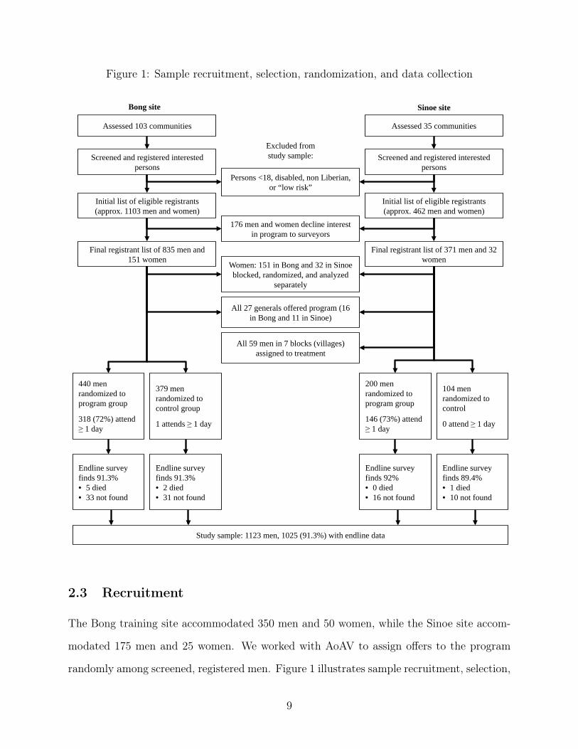
Figure 1: Sample recruitment, selection, randomization, and data collection
Assessed 103 communities
Screened and registered interested persons
Bong site
Initial list of eligible registrants (approx. 1103 men and women)
Persons <18, disabled, non Liberian, or “low risk”
Final registrant list of 835 men and 151 women
176 men and women decline interest in program to surveyors
All 27 generals offered program (16 in Bong and 11 in Sinoe)
440 men randomized to program group
318 (72%) attend ≥ 1 day
379 men randomized to control group
1 attends ≥ 1 day
Assessed 35 communities
Screened and registered interested persons
Sinoe site
Initial list of eligible registrants (approx. 462 men and women)
Final registrant list of 371 men and 32 women
Endline survey finds 91.3% • 5 died • 33 not found
Endline survey finds 91.3% • 2 died • 31 not found
200 men randomized to program group
146 (73%) attend ≥ 1 day
104 men randomized to control
0 attend ≥ 1 day
Endline survey finds 92% • 0 died • 16 not found
Endline survey finds 89.4% • 1 died • 10 not found
Excluded from study sample:
Study sample: 1123 men, 1025 (91.3%) with endline data
Women: 151 in Bong and 32 in Sinoe blocked, randomized, and analyzed
separately
All 59 men in 7 blocks (villages) assigned to treatment
2.3 Recruitment
The Bong training site accommodated 350 men and 50 women, while the Sinoe site accom-
modated 175 men and 25 women. We worked with AoAV to assign offers to the program
randomly among screened, registered men. Figure 1 illustrates sample recruitment, selection,
9
randomization, and data.
From May to October 2009 AoAV advertised the program in community meetings, and
screened and registered interested and eligible people. There was overwhelming interest in the
program among the hotspot population, high-risk or not. AoAV collected extensive data on
war experiences and current economic activities and attempted to register those they deemed
to be the highest-risk men, especially those least served by previous postwar programs. They
excluded people deemed physically incapable of agriculture and non-Liberians.
We have no data on the men screened out, but we observed the process first-hand and
observed mainly low-risk men being turned away (e.g. non-combatants, or well integrated
ex-fighters). Undoubtedly some high-risk men were not interested in the program, so did
not register.
AoAV registered 1,565 men and women and passed them to a baseline survey team.
176 people withdrew their interest or could not be found, resulting in 1,206 registered men
and 183 women. Our experimental analysis excludes 27 high-ranking “generals” who were
automatically offered the program, as the UN considered it too risky to exclude them. We
also exclude women who participated in the program, who were few in number have very
different characteristics and risks.
This screening and self-selection has implications for the interpretation of treatment
effects: they apply to the subset of non-ranking, high-risk men who have some minimum
interest in a training intervention. This is probably the main quantity of academic and policy
interest, however.
2.4 Randomization
To randomize men, we blocked by training site, rank, and community and, within blocks,
assigned each person a uniform random variable and sorted in ascending order. Men were
randomly assigned to an offer to enter the program in this order within blocks until a target
number per block was reached. If a person refused or could not be located, they were still
10
assigned to the treatment group (an offer) and the offer went to the next person on the list.14
Of 1,123 men, 57% were assigned to treatment.
3 Data
Table 1 describes men at baseline.15 On average, the men were aged 30, had 5.9 years of
schooling, with 27% literate. They reported cash earnings of $47 in the past month, savings
of $46, and debts of $7. 74% were in a wartime faction, though only 17% reported being on
the front lines. 13% reported close relations with a former commander.
Most men already were already subsistence farming, as markets were distant and food
expensive. On average they had 4.8 years of farm experience. 32% said farming was their
main source of income, and 29% reported it was non-farm labor or business. 47% reported
some work in illicit activities in the past week, but only 23% said that this was their main
source of income. 87% said they were “very interested” in being a farmer. 90% said they
could easily access 10 acres of land.
The sample was broadly balanced along covariates. Columns 2 and 3 of Table 1 report the
treatment and control group difference in select baseline covariates. Just 7% of all covariates
have an imbalance with p < .1. The treatment group, however, had lower savings and spent
more time in armed factions.16 All treatment estimates control for all covariates.14We adopted this method because AoAV had a fixed number of program spots to fill and a short time
in which to inform and pick up the dispersed men. In Sinoe, 59 men from 7 blocks were dropped from thestudy because their block was fully assigned to treatment. Bridge collapses and construction delays meantthat they received only one or two days notice before pickup, thereby increasing refusal rates such that allmen received the offer.
15See Appendix B.1 for more covariates. Surveyors failed to collect data on 13 (1.2%) men. 5% also optedto skip some sensitive questions on war experiences. We impute the median for missing baseline data.
16A joint test of significance of all 83 baseline covariates has p = .41 excluding these two covariates, butp < .01. including them. Note, however, that other variables related to wealth, debts, armed group activity,and violence have little association with treatment. Moreover, there is little treatment-control difference inpredicted outcomes using baseline covariates (see Appendix B.1). As a result, imbalance is unlikely to be anidentification concern.
11
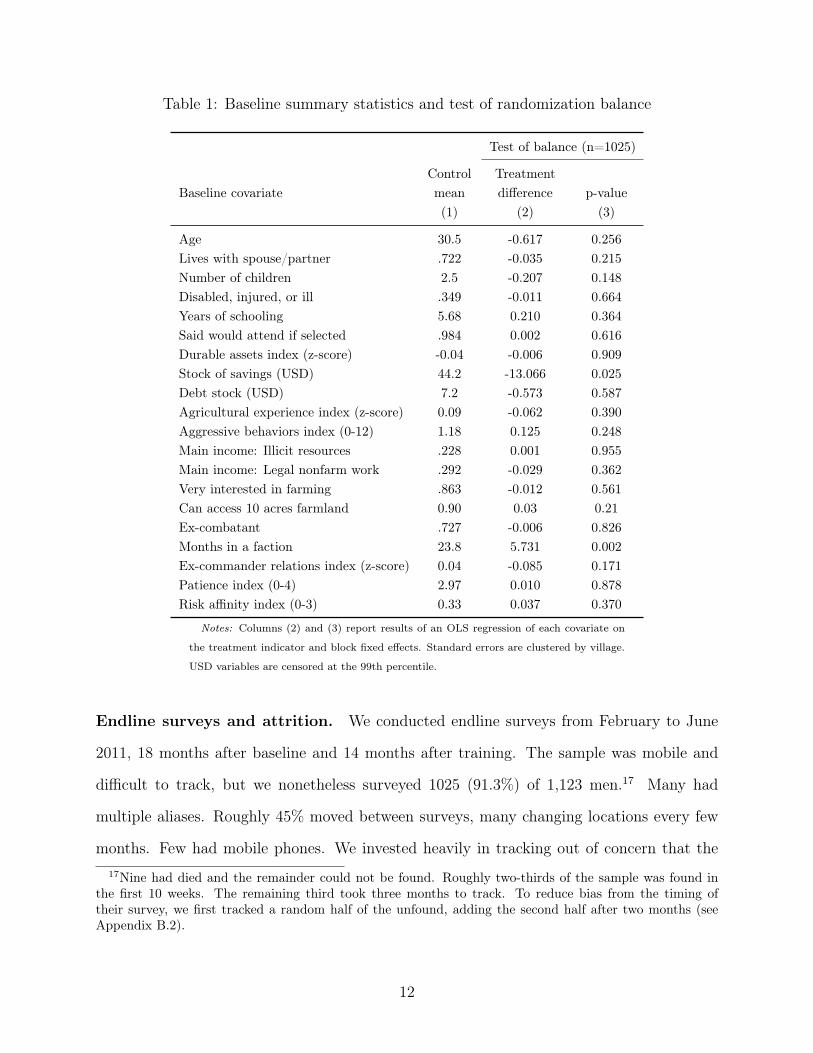
Table 1: Baseline summary statistics and test of randomization balance
Test of balance (n=1025)
Baseline covariateControlmean
Treatmentdifference p-value
(1) (2) (3)
Age 30.5 -0.617 0.256Lives with spouse/partner .722 -0.035 0.215Number of children 2.5 -0.207 0.148Disabled, injured, or ill .349 -0.011 0.664Years of schooling 5.68 0.210 0.364Said would attend if selected .984 0.002 0.616Durable assets index (z-score) -0.04 -0.006 0.909Stock of savings (USD) 44.2 -13.066 0.025Debt stock (USD) 7.2 -0.573 0.587Agricultural experience index (z-score) 0.09 -0.062 0.390Aggressive behaviors index (0-12) 1.18 0.125 0.248Main income: Illicit resources .228 0.001 0.955Main income: Legal nonfarm work .292 -0.029 0.362Very interested in farming .863 -0.012 0.561Can access 10 acres farmland 0.90 0.03 0.21Ex-combatant .727 -0.006 0.826Months in a faction 23.8 5.731 0.002Ex-commander relations index (z-score) 0.04 -0.085 0.171Patience index (0-4) 2.97 0.010 0.878Risk affinity index (0-3) 0.33 0.037 0.370
Notes: Columns (2) and (3) report results of an OLS regression of each covariate on
the treatment indicator and block fixed effects. Standard errors are clustered by village.
USD variables are censored at the 99th percentile.
Endline surveys and attrition. We conducted endline surveys from February to June
2011, 18 months after baseline and 14 months after training. The sample was mobile and
difficult to track, but we nonetheless surveyed 1025 (91.3%) of 1,123 men.17 Many had
multiple aliases. Roughly 45% moved between surveys, many changing locations every few
months. Few had mobile phones. We invested heavily in tracking out of concern that the17Nine had died and the remainder could not be found. Roughly two-thirds of the sample was found in
the first 10 weeks. The remaining third took three months to track. To reduce bias from the timing oftheir survey, we first tracked a random half of the unfound, adding the second half after two months (seeAppendix B.2).
12
hardest to find would be the most prone to violence. We made at least four attempts to
locate each person. To mitigate excess attrition among the untreated, they received a phone
worth $15 for completing the endline.
Attrition is not significantly correlated with treatment, and all baseline covariates explain
just 11 percent of the variation. Some covariates are significantly related, and imply unfound
could be those with a higher propensity for illicit activities and violence—they are slightly
more likely to be ex-combatants, have slightly higher baseline aggression, and have been
illicit rubber tappers.18
Qualitative data. We also conducted eight weeks of unstructured interviews before, dur-
ing, and after the program with participants, community leaders, UN and government per-
sonnel, and non-study residents. Furthermore, under our supervision, one American and two
Liberian research assistants followed 26 treated men over two years, typically interviewing
them four times (before, during and twice after training).19 To understand recruitment ac-
tivities we also conducted informal interviews with ex-fighters and ex-commanders outside
our sample, as well as government and UN personnel, during the crisis in Côte d’Ivoire.
4 Conceptual framework
AoAV designed their intervention to affect occupational choice in three ways. First, they
used training to raise the returns to labor and capital in agriculture. Second, the input
package aimed to relieve a constraint on available capital, with inputs that were difficult
to sell or use in other sectors. Like many DDR and correctional programs, the goal was to
provide material incentives for lawful rather than unlawful work.
A third aspect of the intervention, the counseling and life-skills, aimed at something18See Appendix B.3 for regression results. A test of joint significance of all covariates, however, has p < .01.19They followed semi-structured questionnaires at each stage, with topics including: program experiences,
economic activities, social relationships, war experiences, aggression, and aspirations. In addition to inter-views, research assistants accompanied these individuals to class, to their fieldwork, mealtimes, and freetime. They took detailed notes and recorded and transcribed interviews.
13
less conventional: socialization. The idea was that some actions or professions have direct
utility benefits or penalties—that people have preferences over how their income is earned
(e.g. Akerlof and Kranton, 2000). These preferences are thought to be partly rooted in one’s
self-image, social category, and experiences. By providing education, a new profession, and
relocation, AoAV’s intervention tried to affect occupational choice by changing self-image
and peers, and thus affecting penalties from oneself or peers for deviant behavior.
This section tries to capture these aims in a simple model of occupational choice between
legal and illegal occupations. We outline the framework and key insights here, with full
details in Appendix C.
4.1 Setup
We assume people allocate their labor between leisure l, legal activities La (such as agricul-
ture), and illicit activities Lm (such as unlicensed mining or mercenary work). Legal work
(“agriculture”, for simplicity) is a function of one’s labor, productivity θ (driven by locally-
available technologies and techniques), and capital inputs Xt−1 (such as seeds), which are
decided in the previous period. Agricultural output is thus F (θ, Lat , Xt−1), and AoAV’s
intervention provides inputs and aims to increase productivity.
Meanwhile, we assume mining and mercenary work pays an hourly wage that varies over
time, wt.20 It also comes with a risk of future punishment. For simplicity, we assume this cost
is a linear function of last periods’ hours in mining and mercenary work: ρfLmt−1, where ρ is
the probability of apprehension and f is the punishment. Punishment includes imprisonment
and foregone wages, but it could also include the withholding of a “peace dividend” such as
a cash transfer.21
20In other words, crime principally uses labor as an input. For example, mining requires capital and landrights, and the “bosses” who hold these hire men as “mining boys” on short-term renewable contracts thatpay a daily wage plus a payment tied to output. While there is uncertainty in output, and hence the wage,output is principally a function of labor inputs by the laborer (given a boss’ capital).
21As described below, treated men who chose to specialize in animal-raising expected to receive an in-kindcapital or cash transfer. In this case, ρ is the possibility of missing the transfer if he leaves town to mineor fight, and f the value of the transfer. In principle f could include risk of injury or death, except we’vemodeled it as a transitory shock. Nonetheless a very large f would provide the basic comparative statics.
14
Total earnings from all activities are thus yt ≡ ptF (θ, Lat , Xt−1) +wtLmt − ρfLmt−1, where
p is the price for output. In addition to investing in agricultural inputs, the person can also
invest or borrow through a riskless asset with constant returns 1 + r.22 We can consider the
case where there is no production risk, and also the case where agricultural productivity and
the illicit wage are subject to stochastic shocks.
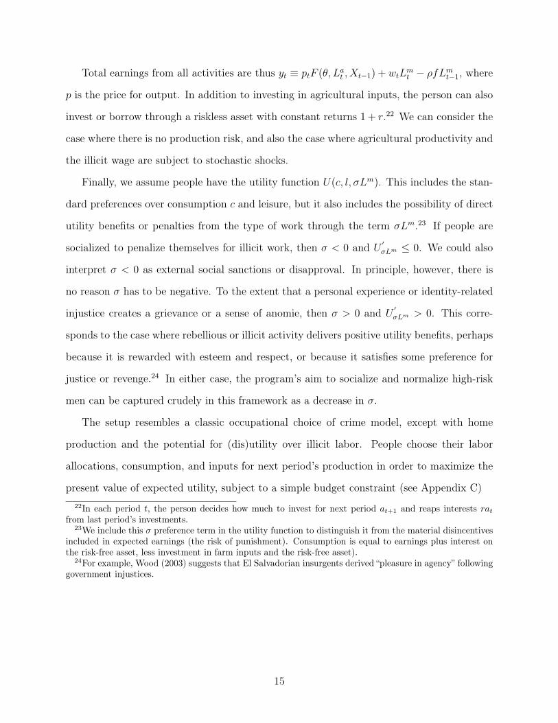
Finally, we assume people have the utility function U(c, l, σLm). This includes the stan-
dard preferences over consumption c and leisure, but it also includes the possibility of direct
utility benefits or penalties from the type of work through the term σLm.23 If people are
socialized to penalize themselves for illicit work, then σ < 0 and U ′σLm ≤ 0. We could also
interpret σ < 0 as external social sanctions or disapproval. In principle, however, there is
no reason σ has to be negative. To the extent that a personal experience or identity-related
injustice creates a grievance or a sense of anomie, then σ > 0 and U′σLm > 0. This corre-
sponds to the case where rebellious or illicit activity delivers positive utility benefits, perhaps
because it is rewarded with esteem and respect, or because it satisfies some preference for
justice or revenge.24 In either case, the program’s aim to socialize and normalize high-risk
men can be captured crudely in this framework as a decrease in σ.
The setup resembles a classic occupational choice of crime model, except with home
production and the potential for (dis)utility over illicit labor. People choose their labor
allocations, consumption, and inputs for next period’s production in order to maximize the
present value of expected utility, subject to a simple budget constraint (see Appendix C)22In each period t, the person decides how much to invest for next period at+1 and reaps interests rat
from last period’s investments.23We include this σ preference term in the utility function to distinguish it from the material disincentives
included in expected earnings (the risk of punishment). Consumption is equal to earnings plus interest onthe risk-free asset, less investment in farm inputs and the risk-free asset).
24For example, Wood (2003) suggests that El Salvadorian insurgents derived “pleasure in agency” followinggovernment injustices.
15
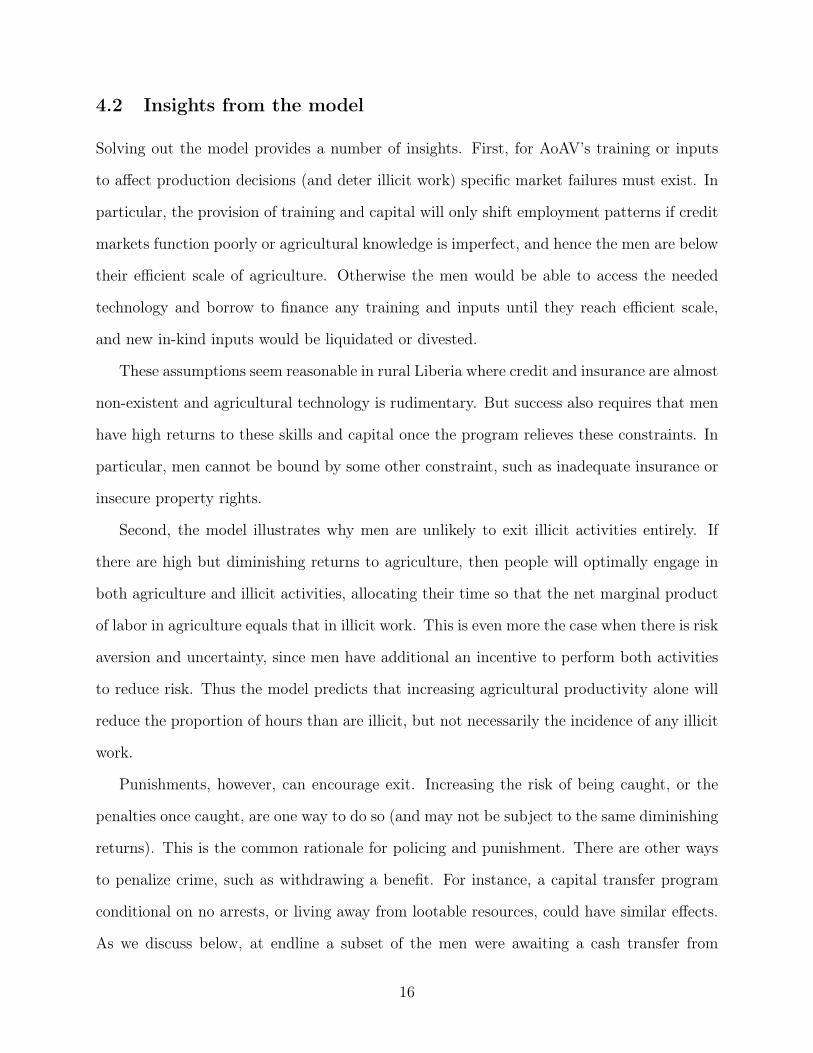
4.2 Insights from the model
Solving out the model provides a number of insights. First, for AoAV’s training or inputs
to affect production decisions (and deter illicit work) specific market failures must exist. In
particular, the provision of training and capital will only shift employment patterns if credit
markets function poorly or agricultural knowledge is imperfect, and hence the men are below
their efficient scale of agriculture. Otherwise the men would be able to access the needed
technology and borrow to finance any training and inputs until they reach efficient scale,
and new in-kind inputs would be liquidated or divested.
These assumptions seem reasonable in rural Liberia where credit and insurance are almost
non-existent and agricultural technology is rudimentary. But success also requires that men
have high returns to these skills and capital once the program relieves these constraints. In
particular, men cannot be bound by some other constraint, such as inadequate insurance or
insecure property rights.
Second, the model illustrates why men are unlikely to exit illicit activities entirely. If
there are high but diminishing returns to agriculture, then people will optimally engage in
both agriculture and illicit activities, allocating their time so that the net marginal product
of labor in agriculture equals that in illicit work. This is even more the case when there is risk
aversion and uncertainty, since men have additional an incentive to perform both activities
to reduce risk. Thus the model predicts that increasing agricultural productivity alone will
reduce the proportion of hours than are illicit, but not necessarily the incidence of any illicit
work.
Punishments, however, can encourage exit. Increasing the risk of being caught, or the
penalties once caught, are one way to do so (and may not be subject to the same diminishing
returns). This is the common rationale for policing and punishment. There are other ways
to penalize crime, such as withdrawing a benefit. For instance, a capital transfer program
conditional on no arrests, or living away from lootable resources, could have similar effects.
As we discuss below, at endline a subset of the men were awaiting a cash transfer from
16
AoAV, and we will argue this punishment lens is a useful way to consider their incentives.
Finally, the model suggests who ought to be targeted by agriculture-oriented reintegra-
tion program, in terms of who is more likely to engage in illicit activities but potential to be
influenced by policy: people with low initial productivity but interest in learning (in agricul-
ture, in this case, though the same argument could be made for other peaceful activities);
and who have little capital and are credit constrained.
Also, the model points out that it will be more difficult to persuade men to pick up
agriculture when their disutility of illicit work is low, when the returns to illicit work are
high (such as rising gold prices), and when agricultural input prices are relatively high.
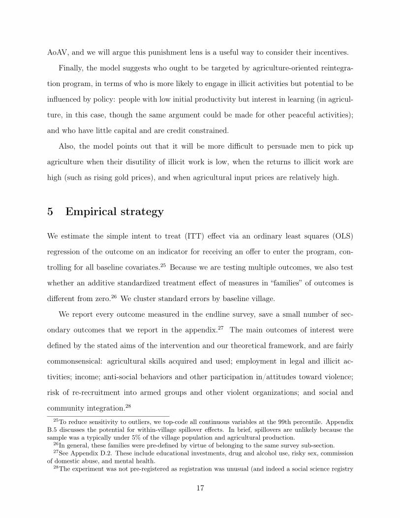
5 Empirical strategy
We estimate the simple intent to treat (ITT) effect via an ordinary least squares (OLS)
regression of the outcome on an indicator for receiving an offer to enter the program, con-
trolling for all baseline covariates.25 Because we are testing multiple outcomes, we also test
whether an additive standardized treatment effect of measures in “families” of outcomes is
different from zero.26 We cluster standard errors by baseline village.
We report every outcome measured in the endline survey, save a small number of sec-
ondary outcomes that we report in the appendix.27 The main outcomes of interest were
defined by the stated aims of the intervention and our theoretical framework, and are fairly
commonsensical: agricultural skills acquired and used; employment in legal and illicit ac-
tivities; income; anti-social behaviors and other participation in/attitudes toward violence;
risk of re-recruitment into armed groups and other violent organizations; and social and
community integration.28
25To reduce sensitivity to outliers, we top-code all continuous variables at the 99th percentile. AppendixB.5 discusses the potential for within-village spillover effects. In brief, spillovers are unlikely because thesample was a typically under 5% of the village population and agricultural production.
26In general, these families were pre-defined by virtue of belonging to the same survey sub-section.27See Appendix D.2. These include educational investments, drug and alcohol use, risky sex, commission
of domestic abuse, and mental health.28The experiment was not pre-registered as registration was unusual (and indeed a social science registry
17
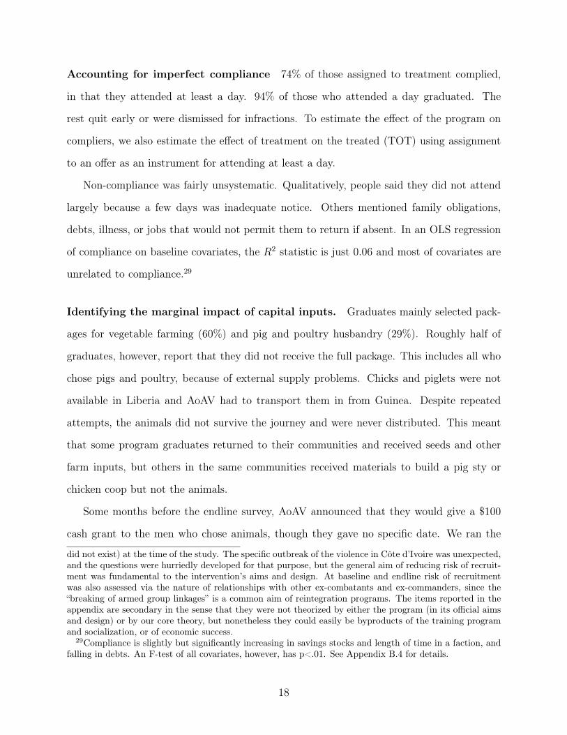
Accounting for imperfect compliance 74% of those assigned to treatment complied,
in that they attended at least a day. 94% of those who attended a day graduated. The
rest quit early or were dismissed for infractions. To estimate the effect of the program on
compliers, we also estimate the effect of treatment on the treated (TOT) using assignment
to an offer as an instrument for attending at least a day.
Non-compliance was fairly unsystematic. Qualitatively, people said they did not attend
largely because a few days was inadequate notice. Others mentioned family obligations,
debts, illness, or jobs that would not permit them to return if absent. In an OLS regression
of compliance on baseline covariates, the R2 statistic is just 0.06 and most of covariates are
unrelated to compliance.29
Identifying the marginal impact of capital inputs. Graduates mainly selected pack-
ages for vegetable farming (60%) and pig and poultry husbandry (29%). Roughly half of
graduates, however, report that they did not receive the full package. This includes all who
chose pigs and poultry, because of external supply problems. Chicks and piglets were not
available in Liberia and AoAV had to transport them in from Guinea. Despite repeated
attempts, the animals did not survive the journey and were never distributed. This meant
that some program graduates returned to their communities and received seeds and other
farm inputs, but others in the same communities received materials to build a pig sty or
chicken coop but not the animals.
Some months before the endline survey, AoAV announced that they would give a $100
cash grant to the men who chose animals, though they gave no specific date. We ran the
did not exist) at the time of the study. The specific outbreak of the violence in Côte d’Ivoire was unexpected,and the questions were hurriedly developed for that purpose, but the general aim of reducing risk of recruit-ment was fundamental to the intervention’s aims and design. At baseline and endline risk of recruitmentwas also assessed via the nature of relationships with other ex-combatants and ex-commanders, since the“breaking of armed group linkages” is a common aim of reintegration programs. The items reported in theappendix are secondary in the sense that they were not theorized by either the program (in its official aimsand design) or by our core theory, but nonetheless they could easily be byproducts of the training programand socialization, or of economic success.
29Compliance is slightly but significantly increasing in savings stocks and length of time in a faction, andfalling in debts. An F-test of all covariates, however, has p<.01. See Appendix B.4 for details.
18
endline survey shortly before disbursal.
We can use this supply interruption to compare the impacts of receiving training and
inputs versus training and a promise of a cash transfer in the near future. While the inter-
ruption was exogenous, men’s choice of animal versus farm input packages was not. We can
interpret any difference as causal if we think selection of package is exogenous conditional
on observed data.
Conditional unconfoundedness is plausible. Animals have lower cash flow than vegeta-
bles, are more capital intensive, involve less labor, and are perceived to be more profitable.
Thus we might expect more patient, wealthier men with other labor opportunities to choose
animals. But we see no such pattern; the choice of specializations seems to be relatively
uncorrelated with a rich set of baseline covariates. Table 2 report an OLS regression of poul-
try/pig package choice on select baseline covariates among graduates. Only one covariate is
significant: a 1 SD increase in agricultural experience is associated with a 7 percentage point
increase in poultry/pig choice.
19
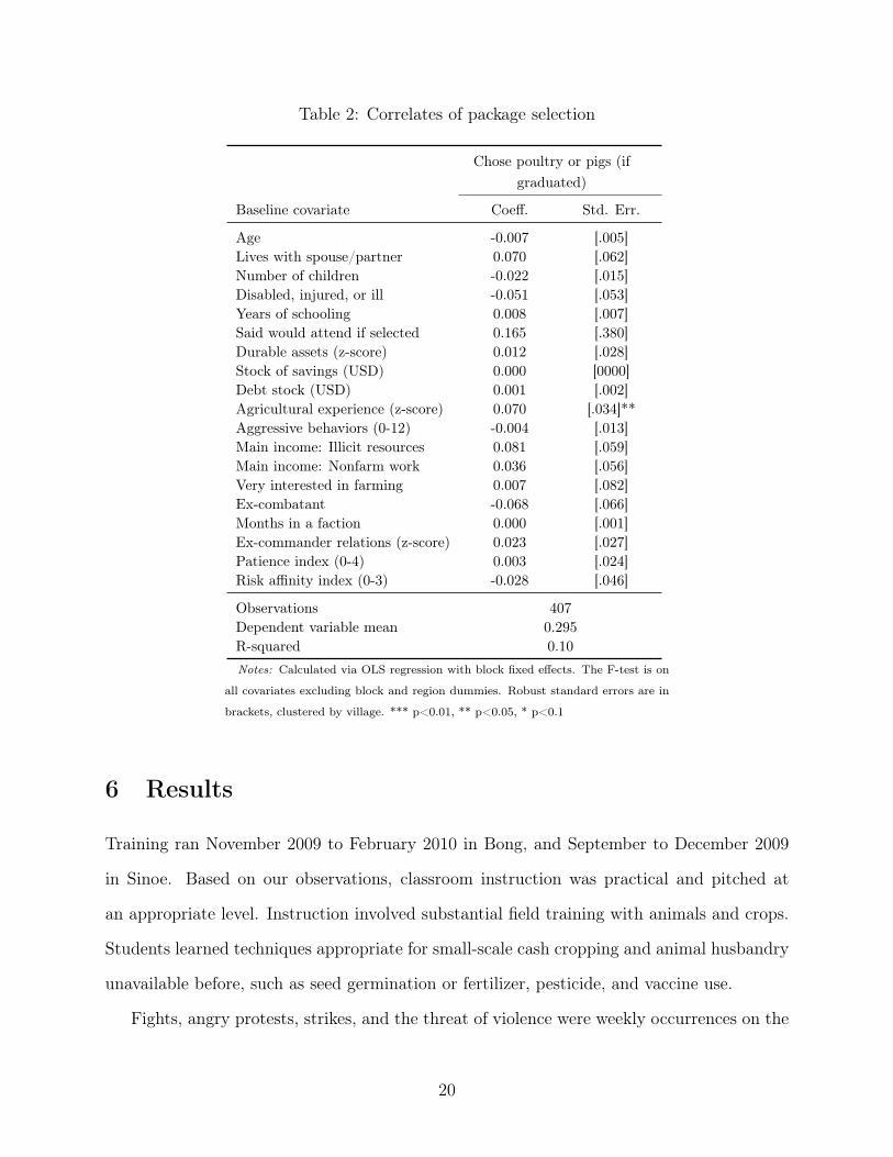
Table 2: Correlates of package selection
Chose poultry or pigs (ifgraduated)
Baseline covariate Coeff. Std. Err.
Age -0.007 [.005]Lives with spouse/partner 0.070 [.062]Number of children -0.022 [.015]Disabled, injured, or ill -0.051 [.053]Years of schooling 0.008 [.007]Said would attend if selected 0.165 [.380]Durable assets (z-score) 0.012 [.028]Stock of savings (USD) 0.000 [0000]Debt stock (USD) 0.001 [.002]Agricultural experience (z-score) 0.070 [.034]**Aggressive behaviors (0-12) -0.004 [.013]Main income: Illicit resources 0.081 [.059]Main income: Nonfarm work 0.036 [.056]Very interested in farming 0.007 [.082]Ex-combatant -0.068 [.066]Months in a faction 0.000 [.001]Ex-commander relations (z-score) 0.023 [.027]Patience index (0-4) 0.003 [.024]Risk affinity index (0-3) -0.028 [.046]
Observations 407Dependent variable mean 0.295R-squared 0.10Notes: Calculated via OLS regression with block fixed effects. The F-test is on
all covariates excluding block and region dummies. Robust standard errors are in
brackets, clustered by village. *** p<0.01, ** p<0.05, * p<0.1
6 Results
Training ran November 2009 to February 2010 in Bong, and September to December 2009
in Sinoe. Based on our observations, classroom instruction was practical and pitched at
an appropriate level. Instruction involved substantial field training with animals and crops.
Students learned techniques appropriate for small-scale cash cropping and animal husbandry
unavailable before, such as seed germination or fertilizer, pesticide, and vaccine use.
Fights, angry protests, strikes, and the threat of violence were weekly occurrences on the
20
training sites. While the events were disruptive, they were also opportunities for the students
to learn to work out grievances peacefully and apply lessons from the life skills class.
Overall, students were enthusiastic about the life skills and counseling. In interviews a
year later, they frequently brought up slogans and examples from the class, and its impact
on their lives. In the endline survey, when asked what part of the program most changed
their life, 23% of graduates said the life skills curriculum and 19% said counseling, compared
to 44% who said skills training and 3% who said inputs.
More than half of graduates chose to return to their baseline community, and most others
chose a community in the same county. Across Liberia farmland is plentiful and arranging
for a few acres of land was straightforward. Community members often said they were proud
of their new or returned residents.
Graduates faced steep challenges, however. They typically returned to remote communi-
ties with sizable local markets but difficult road access and limited access to external markets
and inputs. Furthermore, graduates reported serious liquidity constraints, and hence little
access to tools and inputs beyond what AoAV provided. Farmland was plentiful but typ-
ically rugged, semi-cleared rainforest. Liberian farmers seldom have access to plows, draft
animals, or tractors and perform most work by hand. Pests and rainfall are also persistent
challenges. Program impacts need to be considered in light of these difficulties.
6.1 Impacts on occupational choice and incomes
Table 3 reports control group means and treatment effects for economic outcomes. We focus
on TOT estimates. Men typically had a portfolio of occupations. Illicit opportunities were
often distant from village settlements, and so it was common for men to farm some weeks
of the year in their base village, leave for petty trading, then move elsewhere to mine, log
or tap rubber for a period. Changes in occupation often meant spending fewer days in “the
bush” illicitly mining, and more days in town farming or trading.
The program led to large increases in agricultural work. 61% of controls said they were
21
engaged in farming or animal-raising, and this increased 15.5 percentage points among the
treated—a 26% rise relative to controls. Treated men also expressed more interest in agri-
culture as a career. Interest in farming was high even without treatment: 95% of controls
said that they could make a good living farming, 78% were interested in farming in future,
and 90% were interested in raising animals. Treated men were no more likely to think that
farming is a good career (since opinion is nearly unanimous) but they were 12 percentage
points more likely to express interest in farming. Hours worked in agriculture increased by
4 hours per week, or 33% relative to controls.30
We also observed a shift on the intensive margin away from illicit resource extraction. We
collected days and hours worked at 15 activities in the previous month (a time of dry season
farming and crop sales). Controls reported 49 hours of work per week, and total hours were
not affected by treatment. But treated men decreased hours of resource extraction by 3.7
(23%) and increased other work by 5 hours, mainly agriculture. Importantly, the treated
did not exit illicit activities completely—40% of control men engaged in any illicit extraction
and this was only 3.2 percentage points lower among the treated, not statistically significant.
Reports of felony crime were rare and perhaps for this reason we saw little effect of treat-
ment. We asked about drug selling and theft (stealing, pickpocketing, and armed robbery)
which we assembled into a standardized index. Only 2% of control men reported drug selling
(usually marijuana) and only about 2% of men reported thievery.31 Treated men were half
as likely to report they sold drugs, not statistically significant. There was little effect of
treatment on self-reported stealing.30Treated men were also farming 2 more acres (48%) than controls, though this was not statistically
significant. Appendix D.1 examines individual farm activities. Treated men were more than twice as likelyto be using improved techniques, such as growing seedlings, and were 43% more likely to have sold crops.
31See Appendix D.1 for a breakdown of the index.
22
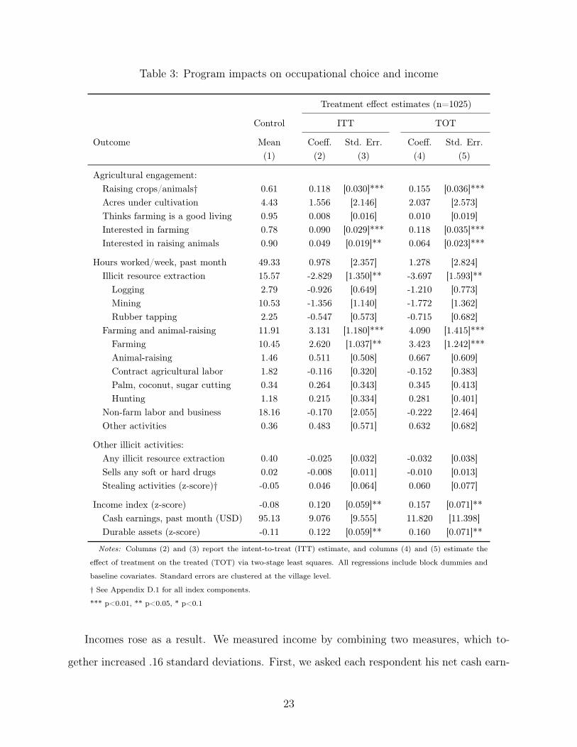
Table 3: Program impacts on occupational choice and income
Treatment effect estimates (n=1025)
Control ITT TOT
Outcome Mean Coeff. Std. Err. Coeff. Std. Err.(1) (2) (3) (4) (5)
Agricultural engagement:Raising crops/animals† 0.61 0.118 [0.030]*** 0.155 [0.036]***Acres under cultivation 4.43 1.556 [2.146] 2.037 [2.573]Thinks farming is a good living 0.95 0.008 [0.016] 0.010 [0.019]Interested in farming 0.78 0.090 [0.029]*** 0.118 [0.035]***Interested in raising animals 0.90 0.049 [0.019]** 0.064 [0.023]***
Hours worked/week, past month 49.33 0.978 [2.357] 1.278 [2.824]Illicit resource extraction 15.57 -2.829 [1.350]** -3.697 [1.593]**Logging 2.79 -0.926 [0.649] -1.210 [0.773]Mining 10.53 -1.356 [1.140] -1.772 [1.362]Rubber tapping 2.25 -0.547 [0.573] -0.715 [0.682]
Farming and animal-raising 11.91 3.131 [1.180]*** 4.090 [1.415]***Farming 10.45 2.620 [1.037]** 3.423 [1.242]***Animal-raising 1.46 0.511 [0.508] 0.667 [0.609]Contract agricultural labor 1.82 -0.116 [0.320] -0.152 [0.383]Palm, coconut, sugar cutting 0.34 0.264 [0.343] 0.345 [0.413]Hunting 1.18 0.215 [0.334] 0.281 [0.401]
Non-farm labor and business 18.16 -0.170 [2.055] -0.222 [2.464]Other activities 0.36 0.483 [0.571] 0.632 [0.682]
Other illicit activities:Any illicit resource extraction 0.40 -0.025 [0.032] -0.032 [0.038]Sells any soft or hard drugs 0.02 -0.008 [0.011] -0.010 [0.013]Stealing activities (z-score)† -0.05 0.046 [0.064] 0.060 [0.077]
Income index (z-score) -0.08 0.120 [0.059]** 0.157 [0.071]**Cash earnings, past month (USD) 95.13 9.076 [9.555] 11.820 [11.398]Durable assets (z-score) -0.11 0.122 [0.059]** 0.160 [0.071]**
Notes: Columns (2) and (3) report the intent-to-treat (ITT) estimate, and columns (4) and (5) estimate the
effect of treatment on the treated (TOT) via two-stage least squares. All regressions include block dummies and
baseline covariates. Standard errors are clustered at the village level.
† See Appendix D.1 for all index components.
*** p<0.01, ** p<0.05, * p<0.1
Incomes rose as a result. We measured income by combining two measures, which to-
gether increased .16 standard deviations. First, we asked each respondent his net cash earn-
23
ings in the past four weeks, activity by activity.32 This earnings measure may be subject to
recall and other biases, and does not capture home production. Also, agricultural incomes
may not have been earned in the past month. We approximate a measure of permanent
income using durable assets—a standardized index constructed by taking the first principal
component of 42 measures of land, housing quality, and durable household assets.
Controls reported $95 in earnings in the month prior to the survey, and this was $11.82
higher among treated men, a 12% increase (not significant, in part because of high variance).
Treated men also reported a 0.16 standard deviation increase in the durable assets index,
significant at the 5% level. The family index of both is statistically significant. This durable
asset increase is likely a result of previous harvests (of which there were 2–3 since the end
of the training program), and is probably a more reliable guide to income than earnings.
In general, these results are robust to alternate treatment effects specifications and at-
trition bounds (see Appendix D.3).
Returns. In the simplest case, we imagine the $11.82 earnings treatment effect represents
a permanent increase in monthly income—$141 annually. This is 11% of the per person
program cost of $1275, and is the cost of capital at which a $141 perpetuity breaks even.
This is not an especially high or rapid private return. Moderate social externalities, however,
could make it a more promising social investment. In this case, the intervention allowed the
government to reclaim resource concessions and, as we see next, may have reduced the risk
of future rebellion.
6.2 Impact on mercenary recruitment activities
We ran our endline survey at a time of escalating violence in Côte d’Ivoire (CI). The in-
cumbent president, Laurent Gbagbo, lost but disputed a November 2010 election to his rival
Alassane Ouattara. Both sides began mobilizing armed forces in December, and there were32Net of expenses, including earnings received, cash earned but as yet unpaid, and the estimated value of
any in-kind payment.
24
sporadic outbreaks of violence through February 2011. Serious fighting began in February
near the Liberian border. Full-scale war broke out by March. By early April, however,
French and UN forces helped to capture and defeat Gbagbo, and hostilities suddenly ceased.
Both sides were accused of recruiting Liberian ex-fighters. Undetermined numbers crossed
from Liberia to Côte d’Ivoire starting in December 2010. About 10,000 Liberian mercenaries
fought in Côte d’Ivoire during 2002-07 hostilities (ICG, 2011). Our qualitative work and news
reports suggest that, by March 2011, no more than 500 Liberian mercenaries had crossed
to Côte d’Ivoire. These men were primarily from the capital and border towns, were some
of the most experienced ex-fighters, and were offered $500 to $1500 to join (ICG, 2011).
According to one Liberian recruit, “Some of us are not working. Our government [in Liberia]
disarmed us, but they have refused to take us into the new army” (Garnaglay, 2011). “We
have been in this business for many years," another said. "We know how to fight well and if
Gbagbo or Ouattara’s men can employ us to fight, that will be good.” Several sources—news
reports, our informal conversations with peacekeepers, ethnographers, and government, and
finally our qualitative interviews with high-risk men during the rising violence—generally
suggest that most interest in recruitment was opportunistic.
Though they undoubtedly exist, it was difficult to find first- or second-hand accounts of
Liberians driven by solidarity or ideology. With the possible exception of the Krahn group
(Guère on the Ivorian side), few Liberian ethnic groups had strong ties to one side or the
other. The Krahn/Guère held close ties to Gbagbo, however, and their area on the Ivorian
side had especially intense violence, took the longest to calm down, and had the most credible
rumors of mercenaries.
To the best of our knowledge, none of our sample went to fight in Côte d’Ivoire. This
is not surprising given the small numbers that went before the war came to a sudden end.
Systematic data on who recruited, and who was recruited, does not exist. Based on our
qualitative interviews, some ex-commanders recruited through their networks, and had begun
to approach and make offers to ex-fighters to prepare for a longer war. In small communities
25
across Liberia, grassroots recruitment activities also proliferated. People, often former mid-
level commanders and generals, would hold secretive meetings of former fighters in the village.
It’s unclear whether these local mobilizers had formal ties to armed groups in Côte d’Ivoire.
Rumors circulated widely about the sums promised to men to go, and appropriate terms
might be discussed in the meetings. Ex-fighters, if interested, could seek out these meetings,
mobilizers, or (in the extreme) make plans to move to one of the border towns where forces
were expected to amass. Other men were more likely to be recruited by dint of their profession
or location (e.g. in a mining town).
Table 4 lists control means and treatment effects for all 16 self-reported measures in the
survey. Some are very indirect proxies for recruitment, and so we display them in a separate
sub-index and interpret them cautiously. For instance, 66% of control men expressed a
partisan preference for either Gbagbo or Ouattara, and 68% said they talked about the war
with friends.
Other survey questions, however, reflect more direct demand for or supply of offers, and
so are better proxies for interest in recruitment or engagement with recruiters. For instance,
8% said they had been approached to go fight, 10% said they were making plans to move
to the border are, 4% said they were invited to go to a secret recruitment meeting, and 3%
reported attending. 3% also reported being offered money to go. 5% reported they would
go for $1000, and 1% said they had concrete plans to go in the next month.33
45% had also talked with a commander in the past 3 months. They could talk to a
commander for many reasons, of course, but the question is whether a treatment effect reflects
a lower likelihood of talking to commanders for reasons of recruitment. Below we show that
the program had no statistically significant effect on relationships with ex-commanders. This
is one reason we include it in the direct proxies, with these caveats.
12 of the 16 measures (including 9 of the 12 more direct measures) are lower for treated33Only 0.5% were actually found in a Côte d’Ivoire border town at endline, and there is no variation by
treatment status. Including this in our index of direct measures has no effect on the results for the overallrecruitment index (Appendix D.3).
26
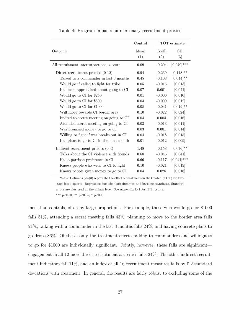
Table 4: Program impacts on mercenary recruitment proxies
Control TOT estimate
Outcome Mean Coeff. SE(1) (2) (3)
All recruitment interest/actions, z-score 0.09 -0.204 [0.079]***
Direct recruitment proxies (0-12) 0.94 -0.239 [0.118]**Talked to a commander in last 3 months 0.45 -0.108 [0.044]**Would go if called to fight for tribe 0.05 -0.015 [0.013]Has been approached about going to CI 0.07 0.001 [0.021]Would go to CI for $250 0.01 -0.006 [0.010]Would go to CI for $500 0.03 -0.009 [0.012]Would go to CI for $1000 0.08 -0.041 [0.019]**Will move towards CI border area 0.10 -0.022 [0.024]Invited to secret meeting on going to CI 0.04 0.004 [0.016]Attended secret meeting on going to CI 0.03 -0.013 [0.011]Was promised money to go to CI 0.03 0.001 [0.014]Willing to fight if war breaks out in CI 0.04 -0.018 [0.015]Has plans to go to CI in the next month 0.01 -0.012 [0.009]
Indirect recruitment proxies (0-4) 1.48 -0.158 [0.076]**Talks about the CI violence with friends 0.68 -0.046 [0.041]Has a partisan preference in CI 0.66 -0.117 [0.041]***Knows people who went to CI to fight 0.10 -0.021 [0.019]Knows people given money to go to CI 0.04 0.026 [0.016]
Notes: Columns (2)-(3) report the the effect of treatment on the treated (TOT) via two-
stage least squares. Regressions include block dummies and baseline covariates. Standard
errors are clustered at the village level. See Appendix D.1 for ITT results.
*** p<0.01, ** p<0.05, * p<0.1
men than controls, often by large proportions. For example, those who would go for $1000
falls 51%, attending a secret meeting falls 43%, planning to move to the border area falls
21%, talking with a commander in the last 3 months falls 24%, and having concrete plans to
go drops 86%. Of these, only the treatment effects talking to commanders and willingness
to go for $1000 are individually significant. Jointly, however, these falls are significant—
engagement in all 12 more direct recruitment activities falls 24%. The other indirect recruit-
ment indicators fall 11%, and an index of all 16 recruitment measures falls by 0.2 standard
deviations with treatment. In general, the results are fairly robust to excluding some of the
27
largest and statistically significant proxies (Appendix D.3).
There are only 21 Krahn in our sample, but the deterrence effect of treatment on merce-
nary interests is larger rather among this ethnic group, suggesting the program was no less
effective when there bonds of solidarity at stake.34
Some results are more difficult to explain, such as the decrease in an expressed partisan
preference with treatment. This could be evidence of the program offer changing political
preferences or grievances. The decision to join an armed group is complex and multifaceted,
and elements of glory, grievances, or other motives were surely present. Thus we cannot
dismiss other, non-material motives.
6.3 In-kind inputs versus an expected cash transfer
These treatment effects conceal heterogeneity in who received the in-kind capital inputs.
Assuming agricultural skills and capital are complements, the model predicts that people
are less likely to increase farming without capital. The effect on illicit activities is ambiguous,
however. In practice, mining and mercenary work requires that men leave the village and
risk missing the disbursement. This could dissuade men from illicit work even if agricultural
returns are low. Missing the disbursement is akin to a punishment in our model.
We estimate the effect of choosing animals in Table 5, which estimates the ITT with
an additional indicator for whether the man chose animals. The coefficient on treatment
alone reflects the effect of choosing farming (columns 1 and 2), the coefficient on the animals
indicator gives the marginal effect of that choice (in columns 3 and 4), and the sum of these
two coefficients is the total program impact on those who chose animals (in columns 5 and
6).
We see that those who chose animals are less likely to increase their agricultural en-
gagement or hours of work. The decrease is not statistically significant, but the decrease in34We present details in Appendix D.4. Similarly strong Liberian ties did not exist for the (largely Muslim)
opposition group, and being Muslim in our sample is a poor predictor of support for the Ivorian oppositionforces.
28
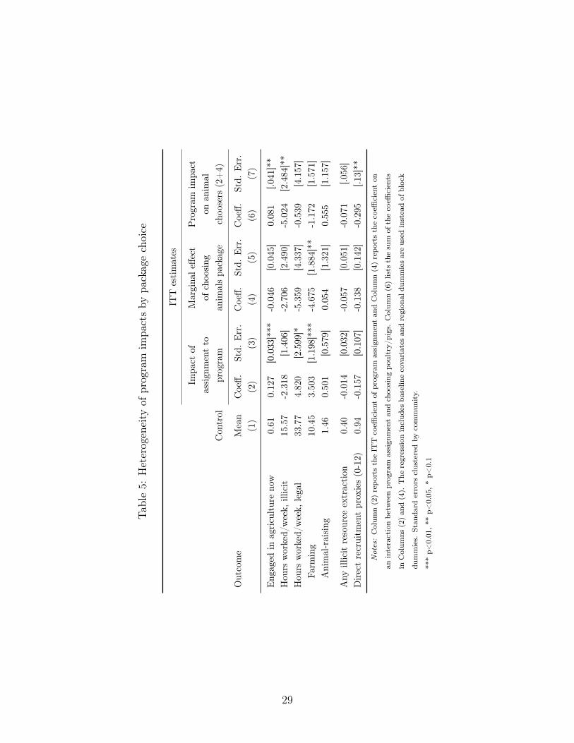
Table5:
Heterogeneity
ofprogram
impa
ctsby
packagechoice
ITT
estimates
Con
trol
Impa
ctof
assign
mentto
program
Margina
leffe
ctof
choo
sing
anim
alspa
ckag
e
Program
impa
cton
anim
alchoo
sers
(2+4)
Outcome
Mean
Coeff.
Std.
Err.
Coeff.
Std.
Err.
Coeff.
Std.
Err.
(1)
(2)
(3)
(4)
(5)
(6)
(7)
Eng
aged
inagricu
ltureno
w0.61
0.127
[0.033]***
-0.046
[0.045]
0.08
1[.0
41]**
Hou
rsworked/
week,
illicit
15.57
-2.318
[1.406]
-2.706
[2.490
]-5.024
[2.484
]**
Hou
rsworked/
week,
legal
33.77
4.820
[2.599]*
-5.359
[4.337
]-0.539
[4.157
]Fa
rming
10.45
3.503
[1.198]***
-4.675
[1.884
]**
-1.172
[1.571
]Animal-raising
1.46
0.501
[0.579]
0.054
[1.321
]0.55
5[1.157
]
Any
illicitresource
extraction
0.40
-0.014
[0.032]
-0.057
[0.051]
-0.071
[.056
]Directrecruitm
entproxies(0-12)
0.94
-0.157
[0.107]
-0.138
[0.142
]-0.295
[.13]**
Not
es:Colum
n(2)repo
rtstheIT
Tcoeffi
cientof
program
assign
mentan
dColum
n(4)repo
rtsthecoeffi
cienton
aninteractionbe
tweenprogram
assign
mentan
dchoo
sing
poultry/
pigs.Colum
n(6)lists
thesum
ofthecoeffi
cients
inColum
ns(2)an
d(4).
The
regression
includ
esba
selin
ecovariates
andregion
aldu
mmiesareused
insteadof
block
dummies.
Stan
dard
errors
clusteredby
commun
ity.
***p<
0.01,**
p<0.05,*p<
0.1
29
hours farming is. Illicit activities fall in both groups, though they appear to fall most in the
animals group (the difference is not statistically significant).
The fall in both illicit resource extraction and mercenary recruitment activities is largest,
however, among those who chose to specialize in animals and were told to expect a transfer.
This is consistent with men staying in villages to await the transfer.35 These estimates
are not sensitive to serious violations of the assumption of conditional unconfoundedness
(Appendix D.3).
6.4 Could results be biased by self-reported data?
One concern with these effects is they use self-reported data. If the treated feel pressure to
report good behaviors (experimenter demand) then we overestimate impacts on them. This
is a challenge in developing countries where administrative data are nonexistent.
Measurement error is a risk, but there are several reasons to think it is a modest one.
First, the patterns we observe are inconsistent with the obvious incentives to misreport.
The counseling and life skills components of the program stressed certain forms of behavior
change: ending use of war names, lowering interpersonal aggression, and solving disputes
peacefully, among other behaviors. Occupational choice, including resource extraction, was
not discussed. Thus if treated men have a tendency to report “good” behavior to surveyors, we
should expect treatment effects to be largest for the behaviors emphasized by their counselors.
Below we will see the opposite is true.
Second, since resource extraction and mercenary actions mainly decrease among animal
choosers, the incentives to misreport would have to be correlated with expecting cash specif-
ically, not treatment in general. While feasible, it is puzzling that we do not see this pattern
appear in the good behaviors explicitly emphasized by the program. Furthermore, the control
group, who were eligible for future training, did not respond to a similar incentive.35This presumes AoAV’s promises were credible after failing to deliver for a year. Our qualitative interviews
suggest that while men were worried about this, most believed AoAV would deliver, largely because theydelivered on previous promises of training, the sty/coop materials, and materials to other men in the villagewho chose vegetables.
30
Third, we attempted to measure social desirability bias in a similar sample. Logistically
it was not possible to validate data for our dispersed, mobile group. Instead, we conducted
a survey validation exercise in the capital among high-risk men in the slums of Monrovia,
especially men engaged in petty crime. These men were part of a field experiment that tested
a similar program of rehabilitation, detailed in Blattman et al. (2015). Briefly, Liberian
qualitative researchers shadowed and interviewed 240 men for four days within ten days of
a written survey. They used in-depth observation, interviews, open-ended questioning, and
efforts at trust-building to elicit more truthful answers about theft, drug use, and gambling
from a random subsample of experimental subjects. Comparing these response to survey
data, we find little evidence of measurement error. If anything, it seems the control group
underreported sensitive behaviors and expenditures, meaning the true treatment effects are
larger than estimated.
6.5 Socio-political impacts
Finally, we see no evidence the program successfully socialized the men differently, including
the aims of the counseling and life skills: peer groups, risky social networks, anti-social
behaviors, community engagement and leadership, and attitudes to violence.
Table 6 reports control group means and TOT estimates for several family indices plus
a subset of the index components as examples (Appendix D.1 lists all components). We
see no evidence the program broke down military chains of command or interaction among
ex-combatants, perhaps because the training intensified exposure to ex-combatants and com-
manders. An index of four measures of ex-combatant relationships increases 0.073 standard
deviations (not significant). An index of relationships with former commanders declines
0.154 standard deviations among treated men (also not significant). Treated men do report
small decreases in close relations with a commander, or receiving support or jobs from a
commander.
We also asked respondents about their closest friends and whether or not they have
31
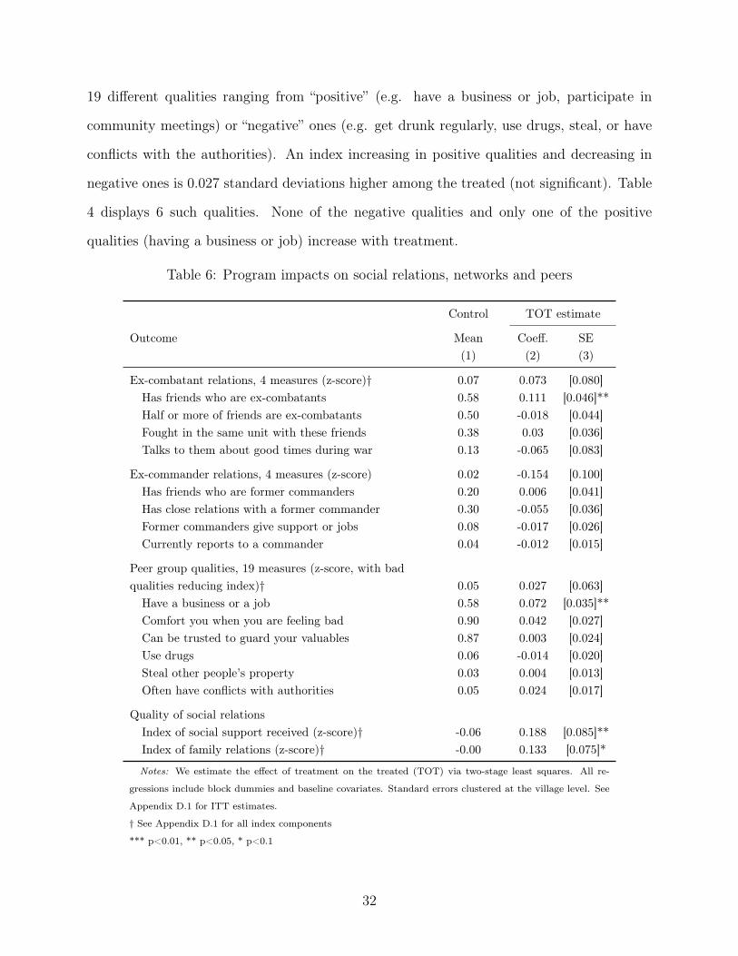
19 different qualities ranging from “positive” (e.g. have a business or job, participate in
community meetings) or “negative” ones (e.g. get drunk regularly, use drugs, steal, or have
conflicts with the authorities). An index increasing in positive qualities and decreasing in
negative ones is 0.027 standard deviations higher among the treated (not significant). Table
4 displays 6 such qualities. None of the negative qualities and only one of the positive
qualities (having a business or job) increase with treatment.
Table 6: Program impacts on social relations, networks and peers
Control TOT estimate
Outcome Mean Coeff. SE(1) (2) (3)
Ex-combatant relations, 4 measures (z-score)† 0.07 0.073 [0.080]Has friends who are ex-combatants 0.58 0.111 [0.046]**Half or more of friends are ex-combatants 0.50 -0.018 [0.044]Fought in the same unit with these friends 0.38 0.03 [0.036]Talks to them about good times during war 0.13 -0.065 [0.083]
Ex-commander relations, 4 measures (z-score) 0.02 -0.154 [0.100]Has friends who are former commanders 0.20 0.006 [0.041]Has close relations with a former commander 0.30 -0.055 [0.036]Former commanders give support or jobs 0.08 -0.017 [0.026]Currently reports to a commander 0.04 -0.012 [0.015]
Peer group qualities, 19 measures (z-score, with badqualities reducing index)† 0.05 0.027 [0.063]Have a business or a job 0.58 0.072 [0.035]**Comfort you when you are feeling bad 0.90 0.042 [0.027]Can be trusted to guard your valuables 0.87 0.003 [0.024]Use drugs 0.06 -0.014 [0.020]Steal other people’s property 0.03 0.004 [0.013]Often have conflicts with authorities 0.05 0.024 [0.017]
Quality of social relationsIndex of social support received (z-score)† -0.06 0.188 [0.085]**Index of family relations (z-score)† -0.00 0.133 [0.075]*
Notes: We estimate the effect of treatment on the treated (TOT) via two-stage least squares. All re-
gressions include block dummies and baseline covariates. Standard errors clustered at the village level. See
Appendix D.1 for ITT estimates.
† See Appendix D.1 for all index components
*** p<0.01, ** p<0.05, * p<0.1
32
Treated men do, however, report better support from existing networks. Table 6 reports
an index of 8 questions about forms of social support received in the past month (such
as people who gave them advice, financial support, etc.) and 7 questions about family
relationships (such as frequency of interaction or whether there are serious disputes). Social
support is 0.19 standard deviations higher among the treated, and the family index is 0.13
standard deviations greater (significant at the 10% level).
Table 7: Program impacts on anti-social behavior and attitudes to violence and democracy
Control TOT estimate
Outcome Mean Coeff. SE(1) (2) (3)
Antisocial behaviors, 13 measures (z-score)† -0.06 0.036 [0.078]Was unable to control your anger (past month) 0.48 0.058 [0.056]Threatened people (past month) 0.10 0.002 [0.035]Took other people’s things (past month) 0.03 0.060 [0.023]***Had a fight or angry dispute (past 6 months) 0.70 0.000 [0.138]
Uses a war name (nom de guerre) 0.32 -0.009 [0.045]
Approval for use of violence, 12 measures (z-score)† -0.05 -0.064 [0.072]Neighbor beats the man who robbed his home 0.08 -0.032 [0.018]*Take things from home of man refusing to repay you 0.04 -0.001 [0.015]Community beats a corrupt leader 0.07 -0.005 [0.019]Community beats policeman bribed to release rapist 0.22 -0.042 [0.033]
Community participation/leadership, 13 measures (z-score)† -0.01 0.112 [0.074]Is a community leader 0.29 -0.024 [0.034]Contributed to care of community water sources 0.67 0.027 [0.043]People often come to you for advice 0.38 0.018 [0.039]Community members come to you to solve disputes 0.28 0.015 [0.039]
Attitudes to democracy, 10 measures (z-score) 7.50 -0.164 [0.131]
Notes: We estimate the effect of treatment on the treated (TOT) via two-stage least squares. All regressions
include block dummies and baseline covariates. Standard errors clustered at the village level. See Appendix D.1
for ITT estimates.
† See Online appendix D.1 for all index components
*** p<0.01, ** p<0.05, * p<0.1
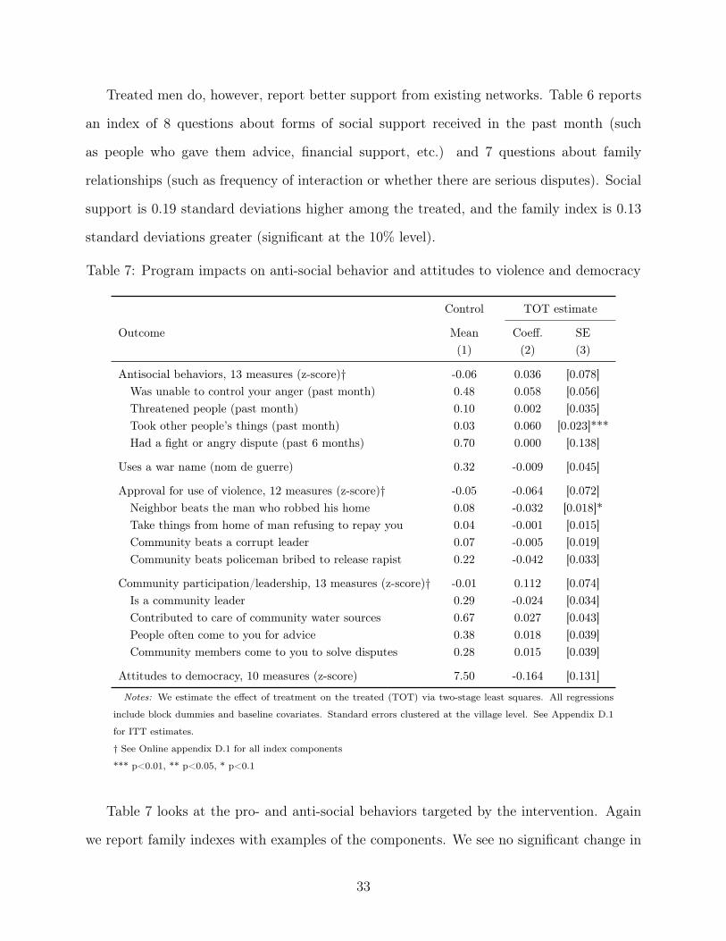
Table 7 looks at the pro- and anti-social behaviors targeted by the intervention. Again
we report family indexes with examples of the components. We see no significant change in
33
an index of 13 questions about aggressive and other anti-social behaviors in the past four
weeks (such as threatening people, destroying their property, or having physical fights). Also,
about a third of the control group use a nom de guerre, a practice actively discouraged by
the facilitators as a symbol of personal change. Treatment has no effect on its use.
We also asked about 12 attitudes towards violence as a means of maintaining order or
justice (such as mob justice). The index is 0.064 standard deviations lower among the treated
(not significant). We asked 13 questions about community participation and leadership (such
as attending community meetings, or contributing to public goods). An index of these is 0.112
standard deviations greater among the treated (not significant). Finally, we see no significant
difference in 10 measures of pro-democratic attitudes, such as whether they disapprove of
military coups when the President’s performance is bad.
7 Discussion and conclusions
There have been few opportunities outside the US to test the effects of labor market interven-
tions on illegal and rebellious activity. This intervention shows that increasing agricultural
productivity and capital led men to shift away from illicit resource extraction on the in-
tensive but not the extensive margin. The extensive margin responded more to future and
ongoing incentives—a conditional cash transfer—rather than a one-time increase in capital
and productivity. These patterns resemble what a simple, standard model of occupational
choice predicts.
Implications for illicit labor markets and economic rehabilitation First, programs
often assume that former fighters, gang members, or other high-risk young men are unin-
terested in traditional occupations like farming. This belief may come from asking young
men “What do you want to be?” rather than “What do you think you will be?” But farming
is the main economic opportunity in Liberia, a point both AoAV and the highest-risk men
understood. Farming is not especially lucrative but it is respectable and commonplace, and
34
indeed necessary for most households for their lifetime. Thus most of them were keen to
improve their knowledge.
Second, the response to the promise of a future cash transfer is insightful. It suggests
that one-time transfers of skills and capital may have limited deterrent effects on future
violence. That is, the most effective peace dividends may pay out repeatedly over time.
Capital transfers or cash-for-work programs could accomplish the same if they condition
payment on men’s location—out of hotspots and not in mercenary work.36
Third, our results are consistent with a growing body of evidence that suggests that
employment programs should emphasize capital alongside skills. Men who received training
and were waiting for their capital were unable to start their farms. This is consistent with our
theoretical model: if people are poor and credit-constrained then the returns to skills alone
will be low. This is also consistent with studies of business skills and vocational training,
which show limited impacts on men and seldom pass a cost-benefit test (e.g. Attanasio
et al., 2011; McKenzie and Woodruff, 2012; Cho et al., 2013). A growing number of studies,
moreover, show that the poor have high returns to capital.37 In the AoAV program, a
reasonable hypothesis is that increasing the availability of capital, or even changing the ratio
of skills to capital provided, would increase cost-effectiveness. This is unknown, however,
and an important question for future study.
Fourth, the elasticity of illegal labor supply suggests the returns to mining and other
resource extraction were not much greater than agriculture to begin with. Given free entry
into illicit resource extraction, it’s perhaps not surprising that returns are competitive with
other opportunities. There are interesting parallels to studies of US drug gangs that finds
that the lowest positions are quite poorly paid, labor supply is elastic, but on the intensive
margin only (Levitt and Venkatesh, 2000). As a result, to persuade men to exit rather than
simply decrease illicit activities, a single-sector focus may be insufficient. Programs that36Cash-for-work can also have a direct “incapacitation” effect, in the same sense that schooling and training
programs are thought to affect crime in large part because they keep high-risk men off the streets (Freeman,1999).
37e.g. Haushofer and Shapiro (2013); Blattman et al. (2014); Banerjee et al. (2015); Blattman et al. (2015).
35
promote both farm and non-farm business (such as petty trading), perhaps by providing
more liquid capital, could reduce risk and hence incentives for illicit work. This is another
important area for research.
Economic incentives might not be enough. The model (and common sense) also imply
that increasing policing and punishment could lead to criminal exit, especially combined with
higher legal wages. Illicit resource extraction was an appealing alternative partly because
of low enforcement. But the aftermath of conflict, it may be easier to change labor market
opportunities than strengthen police forces, at least in the short term.
Implications for theories of armed recruitment The findings are also largely consis-
tent with the idea that armed recruitment responds to material incentives. First, we see large
impacts on returns to legal work (and the opportunity cost of illegal work), but no statisti-
cally significant evidence of impacts on the behaviors and attitudes associated connections to
commanders, peer quality, non-material forms of violence, community participation, or at-
titudes to crime and violence. The program only affected antisocial behaviors with material
incentives. Third, the decrease in both illicit activity and proxies for interest in recruitment
activities is largest among men with future economic incentives not to leave the village.
This is not to say that demand drivers do not matter. Armed social networks, ethnic
solidarity, and grievances undoubtedly influenced men’s interest in mercenary work. And
these drivers may have played an even larger role in a less opportunistic conflict than the
Ivorian one. This general variation in motives is important, but our research design only
identifies the subset of the variation that is affected by the randomized treatment. Like any
source of causal identification, this exogenous variation is not necessarily representative of
all the variation in factors affecting the decision to join an armed group. For the reasons we
outline above, the evidence points to the program affecting material incentives most of all.
One possibility, however, is that getting trained and becoming a successful farmer raised
men’s community esteem and lowered men’s social marginalization. This reduced the appeal
36
of armed groups as a source of respect and upward mobility. We do see that the program
increased social support from friends and family. But there is no significant effect on broader
community participation. Probably economic success and social integration are intertwined,
and a pure economic opportunity cost is too narrow an interpretation of why jobs and income
deter crime and armed recruitment.38
Meanwhile, the one piece of evidence that is consistent with an effect of the program on
grievances is the reduction in expression of a “partisan preference” in the war. This is difficult
to square with a pure opportunity cost motive at work. Relatedly, the one group that had
the closest solidarity with a fighting group were less likely to express interest in recruitment
than their co-ethnics in the control group. But evidence for the opportunity cost mechanism
does not crowd out demand drivers, or vice versa. As our formal model illustrated, they are
likely to be complementary.
Implications for rehabilitation strategies Failure to re-socialize men in this case does
not mean socialization is futile. Indeed, other programs targeting high-risk urban youth, in
both the US and Africa, have successfully changed antisocial behaviors. Successful programs
have tended to target specific behaviors and “character” skills, often using the techniques of
cognitive behavioral therapy, or CBT (Heller et al., 2013; Heckman and Kautz, 2013; Heller
et al., 2015). In urban Liberia, one study shows that eight weeks of non-residential CBT
focused on skills of self-control and a noncriminal self-image had large and sustained impacts
on violence and crime, especially when combined with cash transfers (Blattman et al., 2015).
In the US rehabilitation literature, “best practices” discourage residential programs (since
they do not help people learn to change in their normal environments), and has shown
that concentrating “at-risk” men with “high-risk” men tends to increase antisocial behavior
(Gendreau and Andrews, 1994; Heckman and Kautz, 2013). They also tend to encourage
focused, CBT-style curriculums over lectures or talk therapy. It is possible that a non-
residential program, cognitive-behavioral counseling approach, that treated ex-commanders38See Utas (2003) for a similar argument during reintegration a decade earlier in Liberia.
37
and the highest risk men separately, would have had led to greater social integration. This
too is an important area for more research.
Overall, this paper adds to a growing body of evidence that economic margins matter
for crime and rebellion. As this evidence solidifies, however, it means non-economic ap-
proaches to behavior change are arguably a more important area for future study and policy
experimentation, given the paucity of evidence and uncertainty about what works.
References
Akerlof, G. A. and R. E. Kranton (2000). Economics and identity. Quarterly Journal of
Economics 115 (3), 715–753.
Attanasio, O., A. Kugler, and C. Meghir (2011). Subsidizing Vocational Training for Dis-
advantaged Youth in Colombia: Evidence from a Randomized Trial. American Economic
Journal: Applied Economics 3 (3), 188–220.
Banerjee, A. V. and E. Duflo (2011). Poor economics: A radical rethinking of the way to
fight global poverty. New York: Public Affairs.
Banerjee, A. V., E. Duflo, N. Goldberg, D. Karlan, R. Osei, W. Parienté, J. Shapiro,
B. Thuysbaert, and C. Udry (2015). A Multi-faceted Program Causes Lasting Progress
for the Very Poor: Evidence from Six Countries. Science.
Bazzi, S. and C. Blattman (2014). Economic Shocks and Conflict: Evidence from Commodity
Prices. American Economic Journal: Macroeconomics 6 (4), 1–38.
Becker, G. S. (1968). Crime and Punishment: An Economic Approach. Journal of Political
Economy 76, 169–217. 2.
Berman, E., J. H. Felter, J. N. Shapiro, and M. Callen (2011). Do Working Men Rebel? In-
38
surgency and Unemployment in Afghanistan, Iraq and the Philippines. Journal of Conflict
Resolution 55 (4), 496–528.
Blattman, C., J. Annan, E. P. Green, C. Lehmann, and J. Jamison (2015). The returns
to microenterprise development among the ultra-poor: A field experiment in post-war
Uganda. Working paper .
Blattman, C., N. Fiala, and S. Martinez (2014). Generating skilled employment in developing
countries: Experimental evidence from Uganda. Quarterly Journal of Economics 129 (2),
697–752.
Blattman, C., J. Jamison, and M. Sheridan (2015). Reducing crime and violence: Experi-
mental evidence on adult noncognitive investments in Liberia. Working paper .
Blattman, C. and L. Ralston (2015). Generating employment in poor and fragile states: A
review of the evidence from labor market and entrepreneurship programs. Working paper .
Bøås, M. and A. Hatløy (2008). ‘Getting in, getting out’: militia membership and prospects
for re-integration in post-war Liberia. The journal of modern African studies 46 (01),
33–55.
Cho, Y., D. Kalomba, A. M. Mobarak, and V. Orozco (2013). Gender differences in the
effects of vocational training: Constraints on women and drop-out behavior. Working
paper .
Christensen, M. M. and M. Utas (2008). Mercenaries of Democracy: the ’Politricks’ of
Remobilized Combatants in the 2007 General Elections, Sierra Leone. African Affairs ,
1–25.
Dube, O., O. Garcia-Ponce, and K. Thom (2014). From Maize to Haze: Agricultural Shocks
and the Growth of the Mexican Drug Sector. Working paper .
39
Dube, O. and J. F. Vargas (2013). Commodity Price Shocks and Civil Conflict: Evidence
From Colombia. Review of Economic Studies 80 (4), 1384–1421.
Freeman, R. B. (1999). The Economics of Crime. In O. Ashenfelter and D. Card (Eds.),
Handbook of Labor Economics, Volume 5, pp. 3529–3572. Elsevier.
Garnaglay, B. (2011, January). Liberian mercenaries hope for work in Ivory Coast. Reuters .
Gendreau, P. and D. A. Andrews (1994). The correctional program assessment inventory.
Technical report, University of New Brunswick, Saint John.
Gilligan, M. J., E. N. Mvukiyehe, and C. Samii (2012). Reintegrating Rebels into Civilian
Life: Quasi-Experimental Evidence from Burundi. Journal of Conflict Resolution 57 (4),
598–626.
Grogger, J. (1998). Market Wages and Youth Crime. Journal of Labor Economics 16 (4),
756–791.
Gurr, T. R. (1971). Why Men Rebel. Princeton: Princeton University Press.
Haushofer, J. and J. Shapiro (2013). Welfare Effects of Unconditional Cash Transfers: Evi-
dence from a Randomized Controlled Trial in Kenya. Working paper .
Heckman, J. J. and T. Kautz (2013). Fostering and measuring skills: Interventions that
improve character and cognition. NBER Working Paper 19656 .
Heller, S. B., H. A. Pollack, R. Ander, and J. Ludwig (2013). Preventing Youth Violence
and Dropout: A Randomized Field Experiment. Working Paper .
Heller, S. B., A. K. Shah, J. Guryan, J. Ludwig, S. Mullainathan, and H. A. Pollack (2015).
Thinking, Fast and Slow? Some Field Experiments to Reduce Crime and Dropout in
Chicago. Working paper .
40

Humphreys, M. and J. M. Weinstein (2007). Demobilization and Reintegration. Journal of
Conflict Resolution 51, 531–567. 4.
ICG (2011). Liberia: How Sustainable is the Recovery? Technical report, International
Crisis Group.
Kingma, K. and R. Muggah (2009, May). Critical Issues in DDR: Context, indicators,
targeting, and challenges. Technical report, CIDDR Conference, Colombia.
Levely, I. (2011). Disarmament, Demobilization, Reinsertion and Reintegration in Post-War
Liberia: A failed approach or simply a failed program? Working paper .
Levitt, S. D. and S. A. Venkatesh (2000). An Economic Analysis of a Drug-Selling Gang’s
Finances. Quarterly Journal of Economics 115, 755–789. 3.
McKenzie, D. J. and C. Woodruff (2012). What are we learning from business training and
entrepreneurship evaluations around the developing world? Working paper .
Merton, R. K. (1938). Social Structure and Anomie. American Sociological Review 3, 672–
682. 5.
Miguel, E., S. Satyanath, and E. Sergenti (2004). Economic Shocks and Civil Conflict: An
Instrumental Variables Approach. Journal of Political Economy 112, 725–753. 4.
Nussio, E. and B. Oppenheim (2014). Anti-Social Capital in Former Members of Non-State
Armed Groups: A Case Study of Colombia. Studies in Conflict & Terrorism 37, 999–1023.
Popkin, S. L. (1979). The Rational Peasant: The Political Economy of Rural Society in
Vietnam. Berkeley: University of California Press.
Republic of Liberia (2008). Liberia Poverty Reduction Strategy. IMF Country Report
08/219, Monrovia, Liberia.
Tajima, Y. (2009). Background Paper on Economic Reintegration.
41

Utas, M. (2003). Sweet battlefields: Youth and the Liberian civil war. Uppsala, Sweden:
Uppsala University Dissertations in cultural anthropology. 1.
Walter, B. F. (2004). Does Conflict Beget Conflict? Explaining Recurring Civil War. Journal
of Peace Research 41, 371–88. 3.
Wood, E. J. (2003). Insurgent Collective Action and Civil War in El Salvador. New York:
Cambridge University Press.
World Bank (2012). World Development Report 2013: Jobs. Washington.
42

Appendix for online publication
A Program, curriculum, and budget details
This section details the nature, content, and cost of the program. Table A.1 reports statistics
on program attendance and choices.
Table A.1: Program attendance, performance and choices
Sample
Program choice or outcome
Men assigned to
treatment
Men assigned to
treatment who
attended
Men assigned to
treatment who
graduated
Attended >1 day of training 74%
# training days completed 83.74 113.03 117.63
Graduated 69% 94%
Migrated since baseline 48% 46% 46%
Received part 1 of package 65% 88% 93%
Received part 2 of package 34% 46% 49%
Chose vegetable package 60%
Chose poultry or pigs package 28%
Chose rubber package 7%
Chose other package 5%
% that received both packages:
Chose vegetable 67%
Chose poultry or pigs 7%
Chose rubber 70%
Chose other 48%
Sold part of packages 5%
Observations 586 433 407
A.1 Agricultural training curriculum
The syllabus for the Bong site (called the Tumutu Agricultural Training Program) has 5
major modules. The learning objectives and outcomes for each module is as follows:
1. Rice production (72 hours). After participating in all the module-training activities
(both theory and practical sessions) the trainee is expected to gain broader knowledge
i

on the growth and development of the rice plant and the use of sustainable agricul-
tural methods in rice production, and link rice production to household/national food
security and markets for sustainable livelihoods. At the end of the six month training
in rice production, the trainee should be able to:
(a) Understand and be able to produce upland and lowland rice
(b) Gain a broader knowledge of the importance of proper management of natural
resources (soil and water) and the environment for sustainable rice farming
(c) Develop swamp beds for rice production
(d) Identify sources/types/quality of rice seed and the advantages of using high quality
seed adapted to the local conditions
(e) Lay out, establish, and maintain a nursery
(f) Understand and implement techniques for transplanting/planting of rice seed
(g) Understand the different growth stages in rice development
(h) Maintain a rice field ensuring sustainable management of soil nutrients and opti-
mum conditions for rice growth
(i) Develop capacity to identify diseases and pests and to implement the necessary
control and or treatment measures
(j) Understand techniques for sustainable and profitable harvesting, processing, and
storage of rice
(k) Understand the importance of markets in rice production systems
2. Rubber culture (72 hours). After participating in all the module-training activ-
ities (both theory and practical sessions) the trainee is expected to develop broader
knowledge on sustainable rubber production through the use of sustainable agricul-
tural methods and develop capacity to practice rubber farming and/or gain skills for
ii
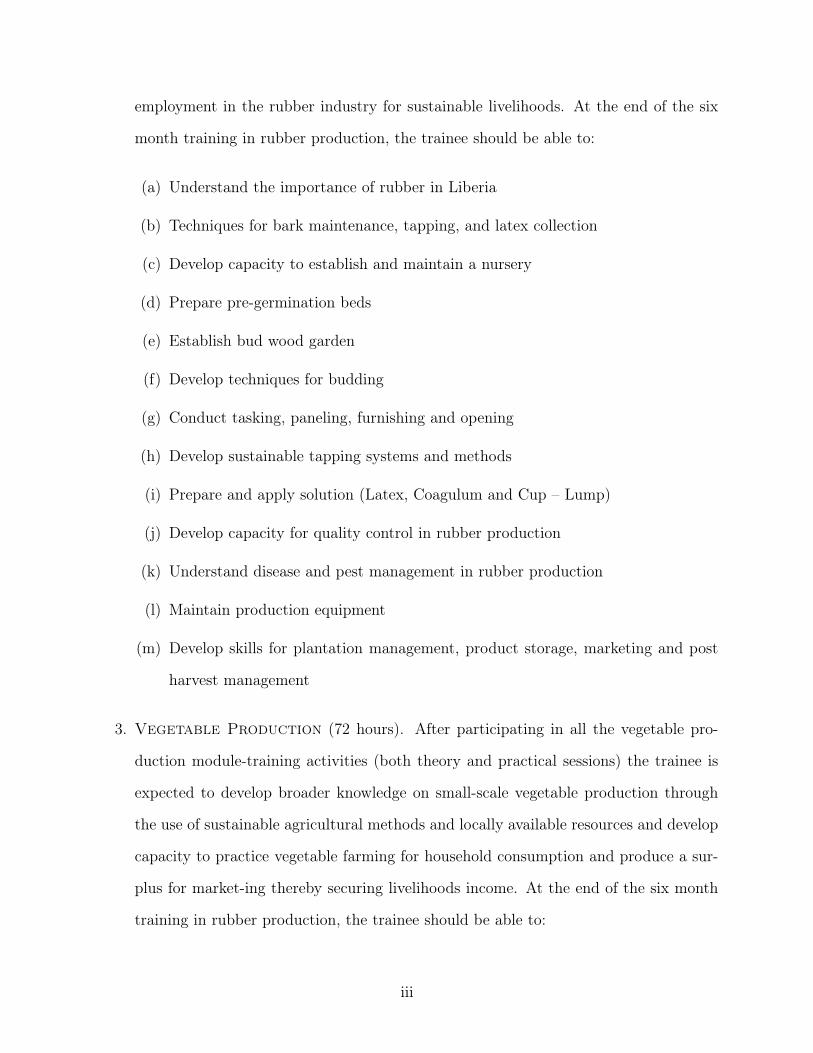
employment in the rubber industry for sustainable livelihoods. At the end of the six
month training in rubber production, the trainee should be able to:
(a) Understand the importance of rubber in Liberia
(b) Techniques for bark maintenance, tapping, and latex collection
(c) Develop capacity to establish and maintain a nursery
(d) Prepare pre-germination beds
(e) Establish bud wood garden
(f) Develop techniques for budding
(g) Conduct tasking, paneling, furnishing and opening
(h) Develop sustainable tapping systems and methods
(i) Prepare and apply solution (Latex, Coagulum and Cup – Lump)
(j) Develop capacity for quality control in rubber production
(k) Understand disease and pest management in rubber production
(l) Maintain production equipment
(m) Develop skills for plantation management, product storage, marketing and post
harvest management
3. Vegetable Production (72 hours). After participating in all the vegetable pro-
duction module-training activities (both theory and practical sessions) the trainee is
expected to develop broader knowledge on small-scale vegetable production through
the use of sustainable agricultural methods and locally available resources and develop
capacity to practice vegetable farming for household consumption and produce a sur-
plus for market-ing thereby securing livelihoods income. At the end of the six month
training in rubber production, the trainee should be able to:
iii

(a) Understand the importance of vegetable production for household and national
food security
(b) Understand and classify types of vegetables
(c) Develop knowledge on the proper usage and maintenance of tools in vegetable
production
(d) Understand the importance of and operate records in vegetable production
(e) Understand the factors considered for vegetable production site selection and
prepare selected land sites for production
(f) Establish and maintain a vegetable nursery
(g) Implement different vegetable production systems
(h) Develop capacity for sustainable disease and pest management
(i) Understand the benefits of organic manuring for sustainable natural resource man-
agement and food quality
(j) Understand compost making and manure selection and application
(k) Understand and develop capacity to harvest different types of vegetables including
quality control and storage
(l) Understand the importance of markets in vegetable production.
4. Tree crops/oil palm (106 hours). After participating in all the tree crops pro-
duction module-training activities (both theory and practical sessions) the trainee is
expected to gain broader knowledge on how to grow oil palms through the use of sus-
tainable agricultural methods and develop capacity to practice oil palm farming as a
cash crop and be in a position to generate an income for long-term sustainable liveli-
hoods. At the end of the six month training in oil palm farming, the trainee will be
expected to:
(a) Understand the importance of oil palm as a cash crop
iv

(b) Understand the required soil and climatic conditions
(c) Be able to select varieties best suited for their communities
(d) Lay out paths and nursery beds and put up shelters in the nursery
(e) Understand factors determining plantation site selection
(f) Carry out pegging of the plantation pattern, planting out the oil palm seedlings
and fencing around the seedlings
(g) Learn how to maintain an oil palm plantation (e.g. cultivation, trimming the
plants, soil nutrient and water management)
(h) Implement sustainable pest and disease management practices
(i) Understand methods of and be able to implement oil palm harvesting, processing
and storage
(j) Understand the importance of markets in oil palm production and develop capac-
ity to access and derive benefits from the market.
5. Animal husbandry (78 hours for poultry, 89 for pigs, and 55 for rabbits). The
training module is designed for beginners to provide fundamental theory of tools, ma-
terials and work practices in animal production (poultry, rabbitory and piggery). After
participating in all the animal husbandry production module-training activities (both
theory and practical sessions) the trainee is expected to gain broader knowledge on how
to keep poultry, rabbits and pigs for household food security and to be in a position
to generate an income through this activity for sustainable livelihoods. At the end of
the training in animal husbandry, the trainee will be expected to:
(a) Develop basic skills for poultry, rabbitory and piggery production
(b) Be able to construct required housing for poultry, rabbits and pigs through the
sustainable use of locally available resources
v
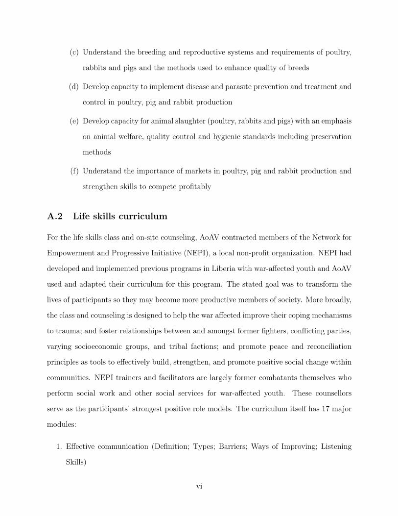
(c) Understand the breeding and reproductive systems and requirements of poultry,
rabbits and pigs and the methods used to enhance quality of breeds
(d) Develop capacity to implement disease and parasite prevention and treatment and
control in poultry, pig and rabbit production
(e) Develop capacity for animal slaughter (poultry, rabbits and pigs) with an emphasis
on animal welfare, quality control and hygienic standards including preservation
methods
(f) Understand the importance of markets in poultry, pig and rabbit production and
strengthen skills to compete profitably
A.2 Life skills curriculum
For the life skills class and on-site counseling, AoAV contracted members of the Network for
Empowerment and Progressive Initiative (NEPI), a local non-profit organization. NEPI had
developed and implemented previous programs in Liberia with war-affected youth and AoAV
used and adapted their curriculum for this program. The stated goal was to transform the
lives of participants so they may become more productive members of society. More broadly,
the class and counseling is designed to help the war affected improve their coping mechanisms
to trauma; and foster relationships between and amongst former fighters, conflicting parties,
varying socioeconomic groups, and tribal factions; and promote peace and reconciliation
principles as tools to effectively build, strengthen, and promote positive social change within
communities. NEPI trainers and facilitators are largely former combatants themselves who
perform social work and other social services for war-affected youth. These counsellors
serve as the participants’ strongest positive role models. The curriculum itself has 17 major
modules:
1. Effective communication (Definition; Types; Barriers; Ways of Improving; Listening
Skills)
vi
2. Perception and role reversal (Definition; Case Study; The Way Forward)
3. Understanding conflict (Definition; Types; Causes; Effects; Tools for Conflict Manage-
ment; Tools for Conflict Resolution)
4. Conflict analysis and transformation (Definition; Strategies; History; People; Tools for
Conflict Analysis & Transformation)
5. Violence and its cycle (Definition; Types; Causes; Effects; Breaking the Cycle of Vio-
lence)
6. Understanding trauma and substance abuse (Effects of Trauma; Definition; Types,
Causes and Effects; The Way Forward)
7. Post-traumatic stress disorder (Definition; Causes; Symptoms and Signs; Developing
Coping Mechanism)
8. Career counseling (Definition; Types; Importance of Career; Career Selection; Two
aspects of Career; Principles for Effective Career)
9. Self image and recovery (Definition; Types; The Building Process)
10. Early warning and early response (Definition, Group Discussion. Mechanism for Pre-
vention & Transformation, The Way Forward
11. Community outlook (Definition; Structure; Norms; Realization & Transformation; Re-
integration)
12. Community initiatives and development (Definition; Types; Ownership and Sustain-
ability)
13. Peace building - Levels and approaches (Definition; Role of a Peace Builder; Peace
Keeping; Peace Making; Peace Building)
vii

14. Challenges of reconciliation (What is Reconciliation?; Steps to Reconciliation; Reli-
gious & Traditional Perspectives of Reconciliation; Dilemmas of Reconciliation; Sus-
taining Reconciliation Work)
15. Leadership styles and skills (What is leadership?; Why is it important?; Can Lead-
ership be Learned?; Best Leader/Role model; Characteristic of Admired Leadership;
Your Leadership Strengths; Seven Critical Leadership Skills; Approaches to Decision
Making)
16. General review
17. Re-entry strategies (Identifying communities for the purpose of possible re-insertion of
trained participants; Confidence building meetings with community leadership; Linking
participants to host communities)
A.3 Example of program budget
Table A.2 reports the budget AoAV submitted (via the UNDP) to the UN Peacebuilding
Fund in 2008 to funding two training courses of 400 students each at the Bong training site.
The first cycle was the focus of the evaluation. Figures reflect the high cost of any operations
and supplies in Liberia, as with many post-conflict regions.
viii
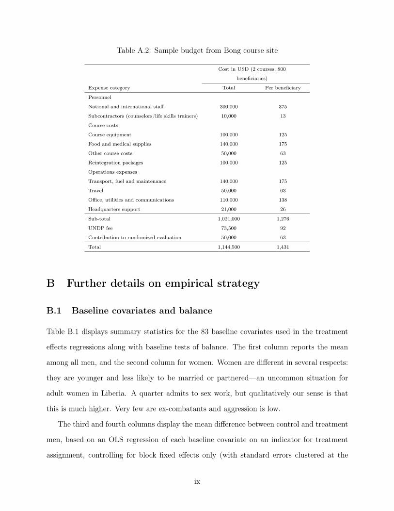
Table A.2: Sample budget from Bong course site
Cost in USD (2 courses, 800
beneficiaries)
Expense category Total Per beneficiary
Personnel
National and international staff 300,000 375
Subcontractors (counselors/life skills trainers) 10,000 13
Course costs
Course equipment 100,000 125
Food and medical supplies 140,000 175
Other course costs 50,000 63
Reintegration packages 100,000 125
Operations expenses
Transport, fuel and maintenance 140,000 175
Travel 50,000 63
Office, utilities and communications 110,000 138
Headquarters support 21,000 26
Sub-total 1,021,000 1,276
UNDP fee 73,500 92
Contribution to randomized evaluation 50,000 63
Total 1,144,500 1,431
B Further details on empirical strategy
B.1 Baseline covariates and balance
Table B.1 displays summary statistics for the 83 baseline covariates used in the treatment
effects regressions along with baseline tests of balance. The first column reports the mean
among all men, and the second column for women. Women are different in several respects:
they are younger and less likely to be married or partnered—an uncommon situation for
adult women in Liberia. A quarter admits to sex work, but qualitatively our sense is that
this is much higher. Very few are ex-combatants and aggression is low.
The third and fourth columns display the mean difference between control and treatment
men, based on an OLS regression of each baseline covariate on an indicator for treatment
assignment, controlling for block fixed effects only (with standard errors clustered at the
ix
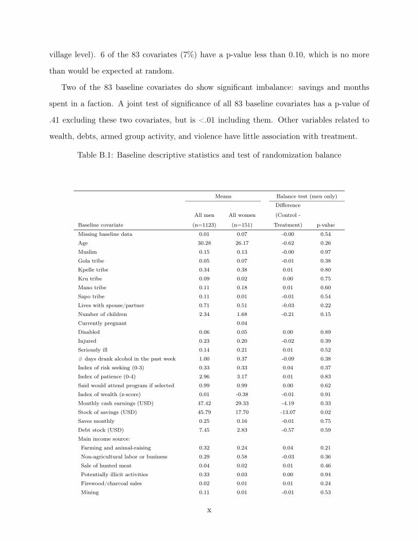
village level). 6 of the 83 covariates (7%) have a p-value less than 0.10, which is no more
than would be expected at random.
Two of the 83 baseline covariates do show significant imbalance: savings and months
spent in a faction. A joint test of significance of all 83 baseline covariates has a p-value of
.41 excluding these two covariates, but is <.01 including them. Other variables related to
wealth, debts, armed group activity, and violence have little association with treatment.
Table B.1: Baseline descriptive statistics and test of randomization balance
Means Balance test (men only)
Baseline covariate
All men
(n=1123)
All women
(n=151)
Difference
(Control -
Treatment) p-value
Missing baseline data 0.01 0.07 -0.00 0.54
Age 30.28 26.17 -0.62 0.26
Muslim 0.15 0.13 -0.00 0.97
Gola tribe 0.05 0.07 -0.01 0.38
Kpelle tribe 0.34 0.38 0.01 0.80
Kru tribe 0.09 0.02 0.00 0.75
Mano tribe 0.11 0.18 0.01 0.60
Sapo tribe 0.11 0.01 -0.01 0.54
Lives with spouse/partner 0.71 0.51 -0.03 0.22
Number of children 2.34 1.68 -0.21 0.15
Currently pregnant 0.04
Disabled 0.06 0.05 0.00 0.89
Injured 0.23 0.20 -0.02 0.39
Seriously ill 0.14 0.21 0.01 0.52
# days drank alcohol in the past week 1.00 0.37 -0.09 0.38
Index of risk seeking (0-3) 0.33 0.33 0.04 0.37
Index of patience (0-4) 2.96 3.17 0.01 0.83
Said would attend program if selected 0.99 0.99 0.00 0.62
Index of wealth (z-score) 0.01 -0.38 -0.01 0.91
Monthly cash earnings (USD) 47.42 29.33 -4.19 0.33
Stock of savings (USD) 45.79 17.70 -13.07 0.02
Saves monthly 0.25 0.16 -0.01 0.75
Debt stock (USD) 7.45 2.83 -0.57 0.59
Main income source:
Farming and animal-raising 0.32 0.24 0.04 0.21
Non-agricultural labor or business 0.29 0.58 -0.03 0.36
Sale of hunted meat 0.04 0.02 0.01 0.46
Potentially illicit activities 0.33 0.03 0.00 0.94
Firewood/charcoal sales 0.02 0.01 0.01 0.24
Mining 0.11 0.01 -0.01 0.53
x
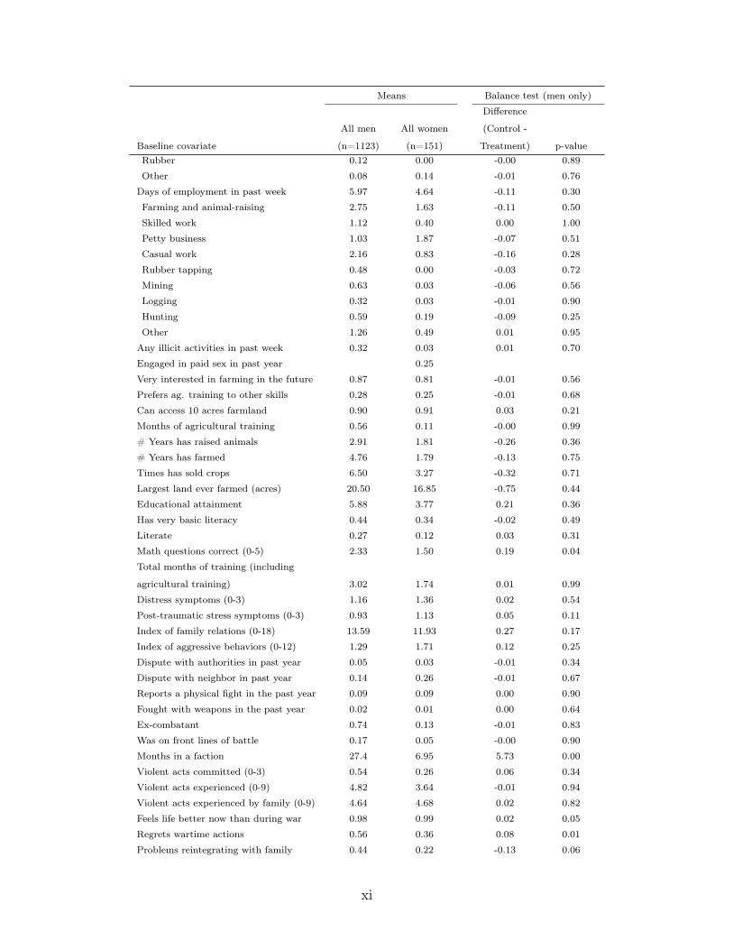
Means Balance test (men only)
Baseline covariate
All men
(n=1123)
All women
(n=151)
Difference
(Control -
Treatment) p-valueRubber 0.12 0.00 -0.00 0.89
Other 0.08 0.14 -0.01 0.76
Days of employment in past week 5.97 4.64 -0.11 0.30
Farming and animal-raising 2.75 1.63 -0.11 0.50
Skilled work 1.12 0.40 0.00 1.00
Petty business 1.03 1.87 -0.07 0.51
Casual work 2.16 0.83 -0.16 0.28
Rubber tapping 0.48 0.00 -0.03 0.72
Mining 0.63 0.03 -0.06 0.56
Logging 0.32 0.03 -0.01 0.90
Hunting 0.59 0.19 -0.09 0.25
Other 1.26 0.49 0.01 0.95
Any illicit activities in past week 0.32 0.03 0.01 0.70
Engaged in paid sex in past year 0.25
Very interested in farming in the future 0.87 0.81 -0.01 0.56
Prefers ag. training to other skills 0.28 0.25 -0.01 0.68
Can access 10 acres farmland 0.90 0.91 0.03 0.21
Months of agricultural training 0.56 0.11 -0.00 0.99
# Years has raised animals 2.91 1.81 -0.26 0.36
# Years has farmed 4.76 1.79 -0.13 0.75
Times has sold crops 6.50 3.27 -0.32 0.71
Largest land ever farmed (acres) 20.50 16.85 -0.75 0.44
Educational attainment 5.88 3.77 0.21 0.36
Has very basic literacy 0.44 0.34 -0.02 0.49
Literate 0.27 0.12 0.03 0.31
Math questions correct (0-5) 2.33 1.50 0.19 0.04
Total months of training (including
agricultural training) 3.02 1.74 0.01 0.99
Distress symptoms (0-3) 1.16 1.36 0.02 0.54
Post-traumatic stress symptoms (0-3) 0.93 1.13 0.05 0.11
Index of family relations (0-18) 13.59 11.93 0.27 0.17
Index of aggressive behaviors (0-12) 1.29 1.71 0.12 0.25
Dispute with authorities in past year 0.05 0.03 -0.01 0.34
Dispute with neighbor in past year 0.14 0.26 -0.01 0.67
Reports a physical fight in the past year 0.09 0.09 0.00 0.90
Fought with weapons in the past year 0.02 0.01 0.00 0.64
Ex-combatant 0.74 0.13 -0.01 0.83
Was on front lines of battle 0.17 0.05 -0.00 0.90
Months in a faction 27.4 6.95 5.73 0.00
Violent acts committed (0-3) 0.54 0.26 0.06 0.34
Violent acts experienced (0-9) 4.82 3.64 -0.01 0.94
Violent acts experienced by family (0-9) 4.64 4.68 0.02 0.82
Feels life better now than during war 0.98 0.99 0.02 0.05
Regrets wartime actions 0.56 0.36 0.08 0.01
Problems reintegrating with family 0.44 0.22 -0.13 0.06
xi
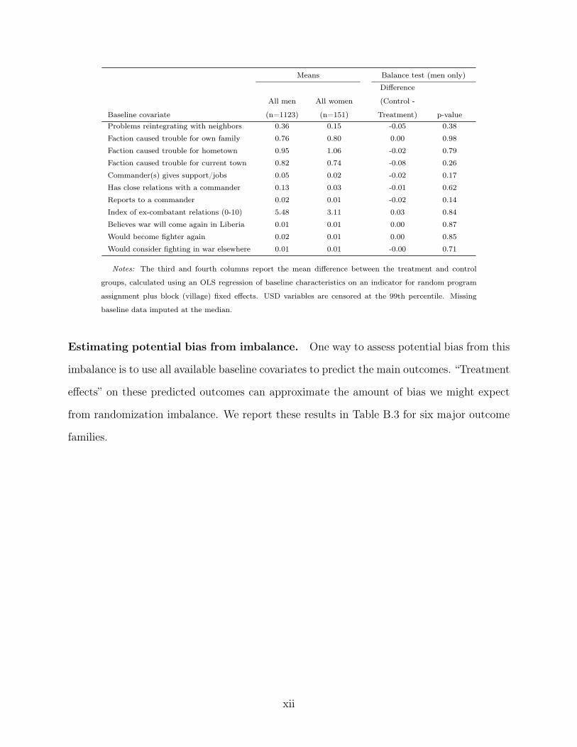
Means Balance test (men only)
Baseline covariate
All men
(n=1123)
All women
(n=151)
Difference
(Control -
Treatment) p-valueProblems reintegrating with neighbors 0.36 0.15 -0.05 0.38
Faction caused trouble for own family 0.76 0.80 0.00 0.98
Faction caused trouble for hometown 0.95 1.06 -0.02 0.79
Faction caused trouble for current town 0.82 0.74 -0.08 0.26
Commander(s) gives support/jobs 0.05 0.02 -0.02 0.17
Has close relations with a commander 0.13 0.03 -0.01 0.62
Reports to a commander 0.02 0.01 -0.02 0.14
Index of ex-combatant relations (0-10) 5.48 3.11 0.03 0.84
Believes war will come again in Liberia 0.01 0.01 0.00 0.87
Would become fighter again 0.02 0.01 0.00 0.85
Would consider fighting in war elsewhere 0.01 0.01 -0.00 0.71
Notes: The third and fourth columns report the mean difference between the treatment and control
groups, calculated using an OLS regression of baseline characteristics on an indicator for random program
assignment plus block (village) fixed effects. USD variables are censored at the 99th percentile. Missing
baseline data imputed at the median.
Estimating potential bias from imbalance. One way to assess potential bias from this
imbalance is to use all available baseline covariates to predict the main outcomes. “Treatment
effects” on these predicted outcomes can approximate the amount of bias we might expect
from randomization imbalance. We report these results in Table B.3 for six major outcome
families.
xii
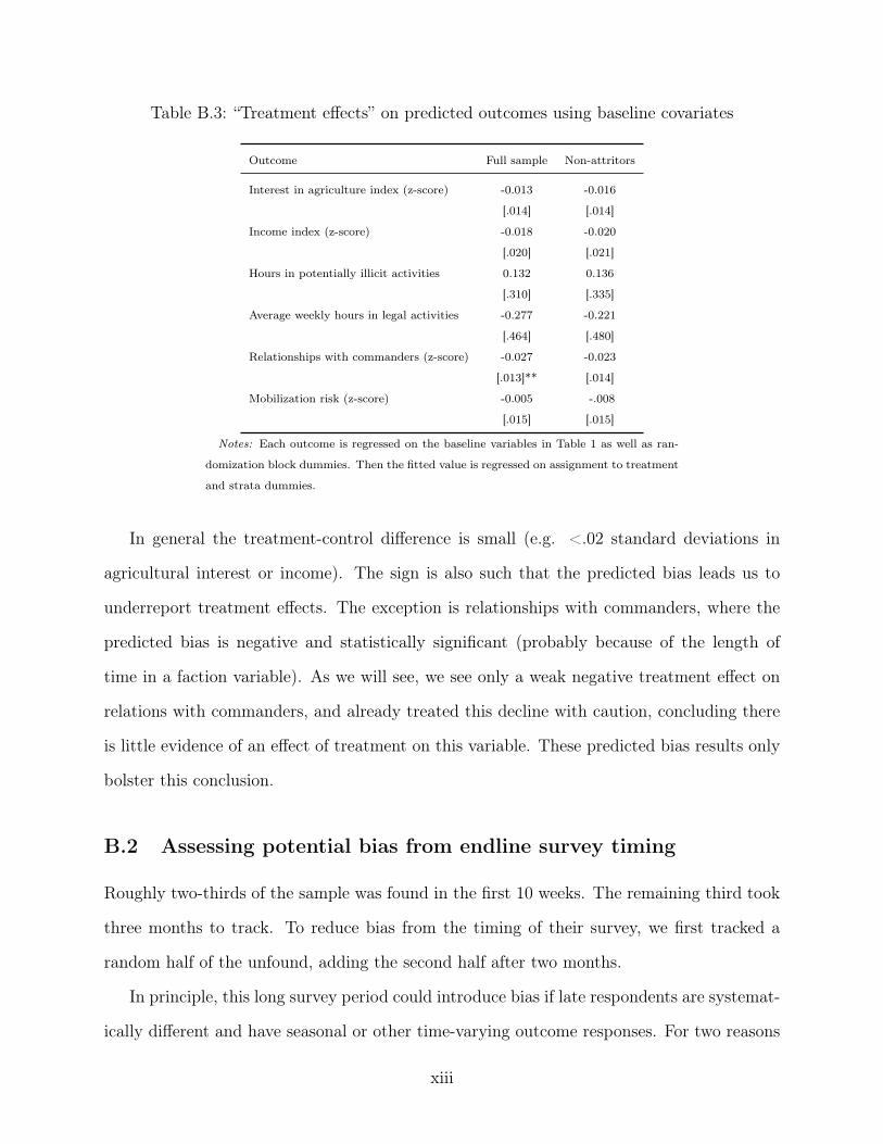
Table B.3: “Treatment effects” on predicted outcomes using baseline covariates
Outcome Full sample Non-attritors
Interest in agriculture index (z-score) -0.013 -0.016
[.014] [.014]
Income index (z-score) -0.018 -0.020
[.020] [.021]
Hours in potentially illicit activities 0.132 0.136
[.310] [.335]
Average weekly hours in legal activities -0.277 -0.221
[.464] [.480]
Relationships with commanders (z-score) -0.027 -0.023
[.013]** [.014]
Mobilization risk (z-score) -0.005 -.008
[.015] [.015]
Notes: Each outcome is regressed on the baseline variables in Table 1 as well as ran-
domization block dummies. Then the fitted value is regressed on assignment to treatment
and strata dummies.
In general the treatment-control difference is small (e.g. <.02 standard deviations in
agricultural interest or income). The sign is also such that the predicted bias leads us to
underreport treatment effects. The exception is relationships with commanders, where the
predicted bias is negative and statistically significant (probably because of the length of
time in a faction variable). As we will see, we see only a weak negative treatment effect on
relations with commanders, and already treated this decline with caution, concluding there
is little evidence of an effect of treatment on this variable. These predicted bias results only
bolster this conclusion.
B.2 Assessing potential bias from endline survey timing
Roughly two-thirds of the sample was found in the first 10 weeks. The remaining third took
three months to track. To reduce bias from the timing of their survey, we first tracked a
random half of the unfound, adding the second half after two months.
In principle, this long survey period could introduce bias if late respondents are systemat-
ically different and have seasonal or other time-varying outcome responses. For two reasons
xiii
this does not appear to be the case in our sample.
First, there is little difference between those found in the first 10 weeks and those who
had migrated and hence took longer to survey and track, implying that timing of the survey
is not too systematically selective. A test of balance between those found before and after
10 weeks (not shown, but available on request) shows that those found after 10 weeks were
a year younger, were 15 percentage points less likely to be married, and were 2 percentage
points less like to be an ex-combatant, but there is no statistically significant difference in
baseline wealth, education, health, occupation, income, aggression, or war experiences.
Second, if we compare treatment effects between men found before and after the 10
weeks, or between the two random groups of unfound men, we see generally the same sign
and magnitude of treatment effects. Results are not displayed but are available on request.
B.3 Attrition
Table B.4 presents results from an ordinary least squares (OLS) regression of attrition (being
unfound) on treatment assignment, covariates, and block fixed effects.
Note that the program appears to have had only a small effect on migration at the time
of the endline. 45% of both the treatment and control group changed villages since baseline,
and 37% moved within the six months before the survey. The control group was slightly
less likely to change their county than treated men: 14% of controls changed their county
and this is 5.7 percentage points higher among treated men, perhaps because they chose to
relocate to more central agricultural markets. 74% of control men also express an interest
in staying in their current community and this settledness is 7.8 percentage points (11%)
higher among treated men.
B.4 Compliance
Table B.4 analyzes the correlates of compliance (attending at least one day). Also, among
those who attend at least one day, it analyzes the correlates of who quits or is dismissed.
xiv
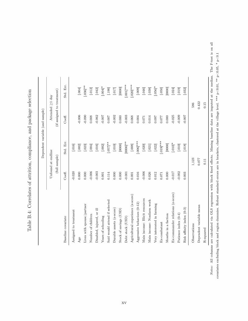
TableB.4:Correlatesof
attrition,
compliance,
andpa
ckageselection
Dep
endent
variab
le(and
sample)
Unfou
ndat
endline
(fullsample)
Attended≥1da
y
(ifassign
edto
treatm
ent)
Baselinecovariate
Coeff.
Std.
Err.
Coeff.
Std.
Err.
Assignedto
treatm
ent
-0.020
[.016]
Age
0.000
[.002]
-0.006
[.004]
Lives
withspou
se/p
artner
0.000
[.023]
-0.090
[.036]**
Num
berof
child
ren
-0.006
[.004]
0.008
[.012]
Disab
led,
injured,
orill
-0.003
[.016]
-0.062
[.042]
Years
ofscho
oling
0.001
[.002]
-0.007
[.004]*
Said
wou
ldattend
ifselected
0.114
[.057]**
0.007
[.190]
Durab
leassets
(z-score)
0.000
[.010]
-0.002
[.017]
Stockof
saving
s(U
SD)
0.000
[0000]
0.000
[0000]
Debtstock(U
SD)
-0.001
[0000]**
-0.003
[.001]***
Agriculturalexpe
rience
(z-score)
0.001
[.008]
0.068
[.020]***
Aggressivebe
haviors(0-12)
0.016
[.006]***
0.004
[.009]
Mainincome:
Illic
itresources
-0.006
[.020]
0.071
[.046]
Mainincome:
Non
farm
work
0.026
[.021]
0.014
[.038]
Veryinterested
infarm
ing
0.012
[.022]
0.097
[.056]*
Ex-comba
tant
0.071
[.019]***
0.077
[.050]
Mon
thsin
afaction
0.000
[0000]
0.000
[0000]
Ex-comman
derrelation
s(z-score)
-0.017
[.010]*
-0.025
[.024]
Patienceindex(0-4)
-0.002
[.010]
-0.009
[.019]
Riskaffi
nity
index(0-3)
0.003
[.018]
-0.007
[.032]
Observation
s1,123
586
Dep
endent
variab
lemean
0.077
0.422
R-squ
ared
0.11
0.15
Not
es:
Allcolumns
arecalculated
viaOLSregression
withblockfix
edeff
ects.
Missing
baselin
eda
taareim
putedat
themedian.
The
F-testis
onall
covariates
exclud
ingblockan
dregion
dummies.
Rob
uststan
dard
errors
arein
brackets,clusteredat
thevilla
gelevel.***p<
0.01,**
p<0.05,*p<
0.1
xv
B.5 Accounting for potential spillover effects
Hotspot communities were limited, and we could not randomize at the community level. It
is possible there are unobserved spillover effects from the treatment group to controls.
For instance, the departure of a small number of high risk men from each community
could reduce the local labor supply and increase wages for illicit work. It could also break
down armed social networks and the power basis of local strongmen, or increase state and
UN presence in the community, thus reducing the returns to illicit work. When the trainees
return, agricultural knowledge could be passed to the control group, increasing their pro-
ductivity. Or successful socialization could influence disutility from illicit labor through peer
effects.
Accurate population figures do not exist, but we estimate treated men typically represent
only 1 to 5% of the adult workforce in these villages. Also, roughly half of both the treatment
and control group changed communities between baseline and endline. Moreover, while
transport costs are high in Liberia, there is considerable migration by this population for
work, especially in mining and local labor supply is highly elastic (implying that we should
not be affected by the departure of a few men). As a result, we expect within-community
spillovers to the control group to be minor. Finally, agricultural hours increase just 20% for
a handful of men per community, and so general equilibrium effects of output on prices seem
extremely unlikely.
Moreover, even if present, the spillovers discussed above should not lead us to overstate
treatment effects. To the extent that the control group become more productive in agricul-
ture, or are influenced by positive peer effects, our estimated treatment effects towards zero
will understate the true program impacts on occupational choice. Any impact on illicit wages
will affect the incentives for both treatment and control group members (although control
group members would be more affected by an increase in w than someone who received
inputs and training).
In principle, individuals who are not assigned to treatment may feel discouraged and
xvi
thus reduce the hours they devote to agriculture, but we see no such trend. Alternatively,
returning farmers could have a negative impact on the control group by crowding them out
of agriculture or if increased output lowered local prices, but qualitatively our assessment is
that production was too small to affect local prices. We do not, however, have the data or
identification to test this formally.
C A model of illegal occupational choice
C.1 Setup
The utility function U(c, l, σLm) has the standard assumptions that U ′c ≥ 0, U ′l ≥ 0, U ′σLm ≤
0 and U ′′cc < 0, U ′′ll < 0, ∂2U/∂L2m ≤ 0.39 The production function F (θ, Lat , Xt−1) also follows
standard assumptions that F ′θ ≥ 0, F ′L ≥ 0, F ′X ≥ 0, F ′′θθ < 0, F ′′LL < 0, F ′′XX < 0, and
F′′
θL ≥ 0, F ′′θX ≥ 0, F ′′LX ≥ 0.40
We begin by ignoring uncertainty and risk aversion. Then we introduce uncertainty in
the form of prices, wages, and productivities following independent stochastic processes. Un-
certainty in prices can reflect variation in general supply and market conditions, uncertainty
in wages can reflect the fact that labor returns are typically conditional on output (e.g. a
minimum wage plus a payment proportional to gold or diamonds discovered or battles won),
and uncertainty in productivity is a simple way of capturing uncertainty in output due to
weather and other unexpected shocks. We keep the assumption that input investment de-
cisions are made one period ahead of production, however we add a new assumption that
decision on hours in both sectors Lat and Lmt are made at time t − 1, one period before all39Examples of utility functions that satisfy these assumptions are U(c, l, σLm) = u(c, l) − σLm and
U(c, l, σLm) = u(c, l)− σ(Lm)2.40 For ease of analysis, we also assume that marginal product of labor in agriculture is zero when there is
no input; but as long as there is some level of input, marginal product of labor for the first unit of labor willbe infinity: F
′
L(θ, La, 0) ≡ 0, but lim
La↓0F
′
L(θ, La, X) = +∞ as long as X > 0. This assumption guarantees
that as long as there is positive investment in inputs, hours in agricultural labor will be positive. We alsoassume that returns to inputs is non-negative but bounded above 0 ≤ F
′
X(θ, La, X) ≤ θM (which is likelythe case in agriculture production).
xvii
prices and productivity levels are realized.
C.2 Benchmark case: Perfect financial markets and no uncertainty
We begin with the case where there are no financial market imperfections. The person’s
problem is
maxct>0,0≤lt≤L̄,Xt,Lmt ,Lat
∞∑t=0
δt [U(ct, lt, σLmt )]
s.t. ct + at+1 + qtXt = yt + (1 + r)at for each t
a0 given
where yt ≡ ptF (θ, Lat , Xt−1) + wtLmt − ρfLmt−1 and Lat + Lmt + lt ≡ L̄.
The first order conditions are as follows:
U′
l (t)
U ′c(t)= ptF
′
La(t) if Lat > 0 (1)
U′
l (t)
U ′c(t)− σU
′σLm(t)
U ′c(t)= wt −
ρf
1 + rif Lmt > 0 (2)
U′c(t)
U ′c(t+ 1)= δ
pt+1
qtF′
X(t+ 1) if Xt > 0 (3)
U′c(t)
U ′c(t+ 1)= δ(1 + r) (4)
ct + at+1 + qtXt = ptF (θ, Lat , Xt−1) + wtLmt − ρfLmt−1 + (1 + r)at (5)
where for ease of notation we use U(t) to denote U(ct, lt, σLmt ) and F (t) to denote F (θ, Lat , Xt−1).
C.2.1 Occupational choice
To find the conditions for engaging in each sector, first consider the case where illicit activity
is not feasible. In this case the decision to engage in agricultural production depends on
his productivity θ, the output-input price ratio pt+1/qt, his wealth level and the returns on
other financial assets r. We use caa, Laa and Xaa to denote consumption, labor and input
xviii

choices in this scenario. In each period t the person chooses Laat to satisfy U′l (c
aat ,L̄−Laat ,0)
U′c(c
aat ,L̄−Laat ,0)
=
ptF′L(θ, Laat , X
aat−1) takingXaa
t−1 as given, and he chooses agricultural investment Xaat to satisfy
pt+1
qtF′X(θ, Laat+1, X
aat ) = 1 + r, taking expected pt+1 and Laat+1 as given.
Now, taking levels of caa, Laa and Xaa as given, we can look at people’ decision to engage
in illicit activities. People will engage in illicit activities if and only if
wt −ρf
1 + r≥ U
′
l (caat , L̄− Laat , 0)
U ′c(caat , L̄− Laat , 0)
+ σ−U ′σLm(caat , L̄− Laat , 0)
U ′c(caat , L̄− Laat , 0)
. (6)
which says the expected returns from illicit activities (wage minus the present value of
expected punishment) must be higher than the highest possible marginal rate of substitution
between leisure and consumption the person can achieve without engaging in illicit activities.
Since −U ′σLm/U′c > 0, a rise in σ means more people will drop out of illicit activities.
If condition 6 is satisfied and ifXt−1 > 0, the person then chooses Lmt and Lat such that the
marginal product of labor in agriculture equals his net marginal gains from illicit activities,
which also equals his marginal rate of substitution between leisure and consumption: i.e.
conditions 1 and 2 will be satisfied. Notice that Lmt may not always be positive. People will
not engage in illicit activities if any or all three of the following happens: (1) wt is very low
relative to price level pt and potential punishment ρf ; (2) productivity in agriculture θ is
very high; and (3) the degree of aversion to illicit activities σ is very high.
Now we come back to the level of Xt. People choose inputs for period t + 1 at time t
with the correct expectation of next period’s prices and wages. Each person chooses Xt such
that investment returns in agriculture and alternative assets are equalized: i.e. condition 3pt+1
qtF′X(θ, Lat+1, Xt) = 1 + r will be satisfied.
Comparative Statics
First, we define the elasticities of illicit labor to the parameters or variables most likely to be
affected by the intervention, θ, X, ρf and σ: εθ = dLmdθ/Lm
θ, εX = dLm
dX/LmX, ερf = dLm
dρf/Lmρf
,
xix

, εσ = dLmdσ/Lmσ. We are also interested in the responsiveness of labor supply to the illicit
wage.
wt
We focus on the case where, as wages wt or the marginal product of labor ptF′L(t) increases,
the substitution effect is greater than the income effect on hours (a reasonable assumption
when both wealth and income are relatively low). If the illicit wage rises, people will engage
in illicit activities as wt surpasses their threshold wage level defined in inequality (6). For
those who already engage in both activities, Lmt rises and Lat falls so that equations (1) and 2
are satisfied. The ratio Lm
Lm+Larises–people are more inclined to engage in illicit activities as
w rises. Then the right hand side of (3) falls (since labor and other inputs are complements),
which means the optimal level of Xt−1 must fall in order to satisfy equations (3) and (4).
Since we assumed substitution effects always dominate income effects, total hours Lat + Lmt
should rise. Total earnings yt ≡ ptF (θ, Lat , Xt−1) + wtLmt would rise as wt rises because
equilibrium returns to both sectors are now higher. Therefore, ∂Lat
∂wt< 0, ∂L
mt
∂wt> 0, ∂Xt−1
∂wt< 0,
∂lt∂wt
< 0 and ∂yt∂wt
> 0. It’s worth noting that because of equations (3) and (4) the returns to
investment in inputs will not change as wt changes, despite the changes in La and X.
ρf
In the absence or risk and uncertainty the effect of an increase in ρf will be the same as the
effect of a fall in wt. Future punishment essentially acts as a monetary penalty to wages in
the illicit sector. Therefore, an increase in ρf will increase agricultural hours and earnings
from agriculture, but reduce hours in illicit activities, total hours, and total earnings: ,∂Lat∂ρf
> 0, ∂Lmt
∂ρf< 0 (i.e. ερf < 0), ∂Xt−1
∂ρf> 0, ∂lt
∂ρf> 0 and ∂yt
∂ρf< 0.
xx

σ
As σ rises, we will see a change in illicit work on the extensive margin: fewer people will
engage in these activities since a higher σ implies a higher right hand side in inequality
(6). For those who already engage in both activities, to keep equation (2) an identity, the
optimal level of Lmt must fall and Lat must rise. The ratio Lm
Lm+Lafalls–people take time
away from illicit activities and put more time into agriculture production. Xt−1 then rises
because of the rise in Lat . The effect on hours and total earnings is less obvious. But holding
everything else constant (i.e. marginal utility of consumption and leisure, wages, prices and
productivity), an increase in σ will lead to a fall in wt+σU′σLm (t)
U ′c(t), which means a lower level of
both U′l (t)
U ′c(t)and marginal productivity of labor ptF
′L(t) in equilibrium. Even though earnings
from agriculture will be higher, the first order effect of σ on Lmt dominates its effects on Lat
, which means ct and yt will be lower in equilibrium, and lt higher. Therefore, ∂Lat∂σ
> 0,∂Lmt∂σ
< 0, εσ < 0, ∂Xt−1
∂σ> 0, ∂lt
∂σ> 0 and ∂yt
∂σ< 0.
θ
Now we consider the effect of an increase in the available agricultural technology θ. On
the extensive margin, fewer people will engage in illicit activities and more will engage in
agriculture activities.41
On the intensive margin, for those who already engage in both activities, the effect of
a rise in productivity level θ is ambiguous. Because of equations (3) and (4), the returns
to investment in inputs will not change (at least so long as we don’t have any financial
constraints or risk). Input level X would rise and labor-input ratio La
Xwill fall. However, the
direction of change in La depends on the shape of production and utility functions as well
as the person’s wealth level. So do the effects on leisure and hours in illicit activities. Both41A higher θ leads to a relatively large increase in caa and an ambiguous but relatively small change in
laa, which together implies a higher right hand side in inequality (6).This is intuitive: as productivity rises,agriculture alone can provide high levels of consumption and leisure for the person such that illicit activitiesdo not seem attractive any more.
xxi

earnings in agriculture and total earnings y will rise. Consumption will rise. If agricultural
production is very labor intensive (which is likely the case), then a rise in θ will lead to a rise
in both La and ptF′L(t), which means a higher level of U
′l (t)
U ′c(t)in equilibrium, and therefore a
lower level of leisure. The effect on Lm depends on the sign of U ′σLm . To sum up, ∂Xt−1
∂θ> 0,
∂yt∂θ
< 0 for certain, and ∂Lat∂θ
> 0 and ∂lt∂θ< 0 if agriculture production is labor intensive and
ambiguous otherwise.
Averaging the effect on both margins, a rise in θ leads to a fall in average Lm and arise in
La. Therefore, Lm
Lm+Lafalls and εθ < 0. Note that an increase in pt (or decrease in qt) would
have similar effects as an increase in θ.
Xt
Since input Xt is a choice variable and there are no financial market imperfections, any
intervention that provides Xt will only have effects in the short-term: reducing returns in
agriculture production to a level below 1 + r, increasing consumption and total earnings,
and reducing hours in illicit activities. The short-term effects on La and l will depend on
the labor intensity of the production function and how important leisure is in the utility
function. However, in the long run, this capital will be divested and everything will go back
to equilibrium levels. In the short run, Lm
Lm+Lafalls and εX < 0; in the long run, Lm
Lm+La
returns to its normal level and εX = 0.
C.3 The case of credit constraints without uncertainty
We consider the simplest case of credit constraints where there is no borrowing whatsoever:
at ≥ 0. Equation (4) becomes U′c(t)
U ′c(t+1)= δ(1 + r) if at > 0 and U
′c(t)
U ′c(t+1)> δ(1 + r) if at = 0.
Combining this with(3), we have
pt+1
qtF′
X(θ, Lat+1, Xt) = max{1 + r,1
δ} (7)
xxii

This implies that fewer people with low wealth will engage in agriculture, and those that do
will invest less in inputs if the credit constraint binds. Unlike the benchmark model, patience
now matters for input decisions: the impatient will now under-invest in agriculture.
In a low wealth sample like ours, compared to the benchmark case, the credit constraint
leads to a lower level of investment X for the impatient types whose δ < 11+r
, fewer hours
in agriculture (lower La), but more hours in illicit activities (higher Lm). Some low patience
people will have to give up agriculture altogether because of the credit constraints. On
average, Lm
La+Lmwill be higher than in the benchmark case.
Interventions in θ and σ will have similar effects as in the benchmark case; εθ and εσ will
have the same signs as in the benchmark case. However, the magnitude of the effects change.
A rise in θ will now have a smaller effect than in the benchmark case, because the credit
constraint makes it harder for everyone to increase their investment in agriculture. On the
contrary, a rise in σ will now have a bigger effect than in the benchmark case, because the
credit constraint makes illicit activities more attractive than in the benchmark case.
Perhaps most importantly, interventions in Xt will now have long-term effects: inducing
people to engage in agriculture activities, and increasing input investments for those who
were credit constrained. εX < 0 both in the long and in the short run. It is worth noting
that in this case giving people ∆Xt amount of inputs should have the exact same effect as
giving them a cash transfer of qt∆Xt.
In other words, εσ < 0, εθ < 0 and εX < 0; the magnitude of εθ and εσ are lower than in
the benchmark case; while εX is higher.
C.4 The case of credit constraints with uncertainty and incomplete
insurance
We now turn to credit constraints in the presence of uncertainty and risk aversion. For
simplicity we assume there is no insurance market, and that the riskless asset remains riskless.
The first order conditions now become
xxiii

Et−1
[U′
l (t)]
= Et−1
[U′
c(t)ptF′
L(t)]
if Lat > 0
Et−1
[U′
l (t)]− Et−1
[σU
′
σLm(t)]
= Et−1
[U′
c(t)wt
]− δEt
[U′
c(t+ 1)]ρf if Lmt > 0
U′
c(t) = δEt[U′
c(t+ 1)pt+1
qtF′
X(t+ 1)
]if Xt > 0
U′
c(t) = δ(1 + r)Et[U′
c(t+ 1)]
if at+1 > 0
ct + at+1 + qtXt = ptF (θ, Lat , Xt−1) + wtLmt + (1 + r)at
Inequality (6), the threshold level of wt that people will engage in illicit activities, now
becomes
Et−1
[U′
c(caat , L̄− Laat , 0)wt
]− δEt
[U′
c(caat+1, L̄− Laat+1, 0)
]ρf ≥
Et−1
[U′
l (caat , L̄− Laat , 0)
]− Et−1
[σU
′
σLm(caat , L̄− Laat , 0)]
and we have another equation for the returns of input investments under uncertainty
Et[pt+1
qtF′
X(θt+1, Lat+1, Xt)
]− (1 + r) = −(1 + r)Covt
(pt+1
qtF′
X(θt+1, Lat+1, Xt), SDt
)(8)
and
(1 + r)
[1 + Covt
(pt+1
qtθt+1M,SDt
)]≤ Et
[pt+1
qtθt+1M
](9)
where SDt =δU′1(t+1)
U′1(t)
is the stochastic discount factor.
Now input X and hours Lm and La all depend both on the variance of returns in the two
sectors and the level of initial wealth a0. Those with high levels of wealth a0 will turn away
from both activities by reducing X, Lm and La and investing instead in other riskless assets
X. Lm and La will all be lower than both the benchmark case and the credit constraint only
case.
People with low levels of wealth (i.e. our sample) will not be able to live off savings alone,
xxiv
so they will have to invest more in both sectors by increasing X, Lm and La if both sectors
are equally risky. Otherwise, if one of the sectors are less risky than the other, people will
invest more time in that sector. Lm
La+Lmwill be higher than in the case without uncertainty
only if illicit activities are less risky than agriculture.
Importantly, interventions in θ will have greater effects than in the benchmark and credit
constraint case, because an increase in θ now also makes agriculture relatively less risky. A
rise in σ will also have a bigger effect than without uncertainty, because risk aversion will
reinforce the rise in aversion and further reduce hours in illicit activities. Inventions in Xt
will have a similar long-term effect as in the credit constraint only scenario. However, for
the risk averse people the effect of ∆Xt will be greater than a cash transfer qt∆Xt. The
effects increase as the level of risk aversion increases, and also as the level of risk increase.
Similarly, a change in either the probability or extent of punishment will have a bigger effect
on hours and earnings: an increase in ρf will make illicit activity even more unattractive, as
it reduces the expected returns to illicit activity while not reducing the risk of such activities.
In other words, εσ < 0, εθ < 0, ερf < 0 and εX < 0; the magnitude of all four elasticities
will be higher than in the credit constraint without uncertainty case.
D Additional treatment effects analysis
D.1 ITT and TOT estimates with all index components
Table D.1 reports intent-to-treat (ITT) impacts of the program on our measures of mercenary
recruitment. Tables D.2 to D.7 expand the family indices that appear in the main paper.
Finally, Tables D.12 and D.13 expand the number of outcomes analyzed for the marginal
impact of package choice.
xxv
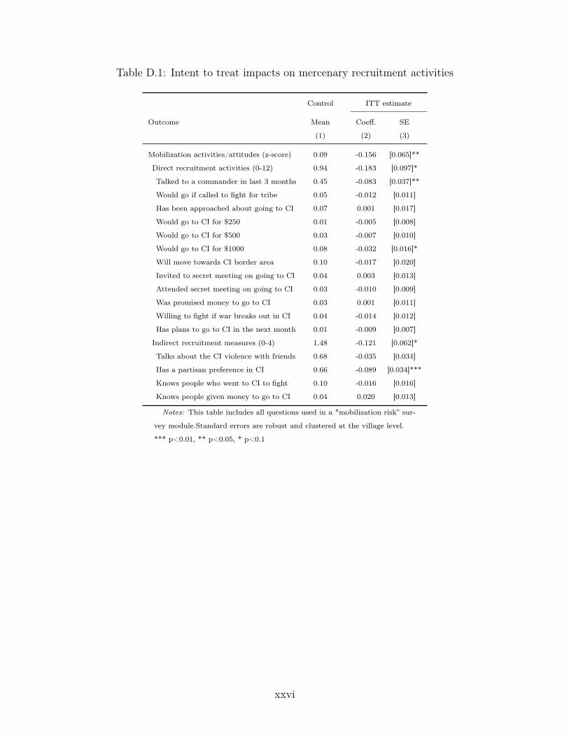
Table D.1: Intent to treat impacts on mercenary recruitment activities
Control ITT estimate
Outcome Mean Coeff. SE
(1) (2) (3)
Mobilization activities/attitudes (z-score) 0.09 -0.156 [0.065]**
Direct recruitment activities (0-12) 0.94 -0.183 [0.097]*
Talked to a commander in last 3 months 0.45 -0.083 [0.037]**
Would go if called to fight for tribe 0.05 -0.012 [0.011]
Has been approached about going to CI 0.07 0.001 [0.017]
Would go to CI for $250 0.01 -0.005 [0.008]
Would go to CI for $500 0.03 -0.007 [0.010]
Would go to CI for $1000 0.08 -0.032 [0.016]*
Will move towards CI border area 0.10 -0.017 [0.020]
Invited to secret meeting on going to CI 0.04 0.003 [0.013]
Attended secret meeting on going to CI 0.03 -0.010 [0.009]
Was promised money to go to CI 0.03 0.001 [0.011]
Willing to fight if war breaks out in CI 0.04 -0.014 [0.012]
Has plans to go to CI in the next month 0.01 -0.009 [0.007]
Indirect recruitment measures (0-4) 1.48 -0.121 [0.062]*
Talks about the CI violence with friends 0.68 -0.035 [0.034]
Has a partisan preference in CI 0.66 -0.089 [0.034]***
Knows people who went to CI to fight 0.10 -0.016 [0.016]
Knows people given money to go to CI 0.04 0.020 [0.013]
Notes: This table includes all questions used in a "mobilization risk” sur-
vey module.Standard errors are robust and clustered at the village level.
*** p<0.01, ** p<0.05, * p<0.1
xxvi
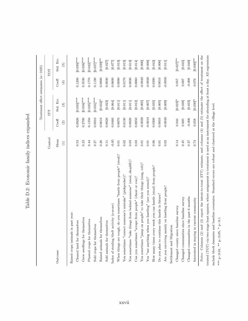
TableD.2:Econo
mic
family
indicesexpa
nded Treatmenteff
ectestimates
(n=1025)
Con
trol
ITT
TOT
Outcome
Mean
Coeff.
Std.
Err.
Coeff.
Std.
Err.
(1)
(2)
(3)
(4)
(5)
Raisedcrop
s/an
imalsin
past
year:
Cleared
land
forthem
selves
0.53
0.0920
[0.033]***
0.1200
[0.039]***
Grew
seedlin
gsforthem
selves
0.23
0.2700
[0.034]***
0.3530
[0.038]***
Planted
crop
sforthem
selves
0.44
0.1350
[0.035]***
0.1770
[0.042]***
Sold
crop
sforthem
selves
0.27
0.0910
[0.031]***
0.1190
[0.037]***
Raisedan
imalsforthem
selves
0.26
0.0610
[0.032]*
0.0800
[0.039]**
Sold
anim
alsforthem
selves
0.11
0.0020
[0.023
]0.0030
[0.027]
Indexof
stealin
g/theftactivity
(z-score)
-0.05
0.0460
[0.064]
0.0600
[0.077]
Whenthings
areroug
h,do
yousometim
es"h
ustlefrom
peop
le"(steal)?
0.01
0.0070
[0.011]
0.0090
[0.013]
You
sometim
es"correct
someone’s
mistake"(pickp
ocket)?
0.02
0.0130
[0.011
]0.0170
[0.013]
You
sometim
es"takethings
from
behind
someone"(steal,shop
lift)?
0.03
0.0020
[0.011]
0.0030
[0.013]
Can
yousometim
es"scrap
efrom
peop
le"(cheat
orcon)?
0.03
0.0050
[0.012]
0.00
60[0.014]
You
sometim
es"jum
pon
peop
le"to
take
theirthings
(mug
,rob)?
0.01
-0.0030
[0.005]
-0.0040
[0.006]
You
"use
anything
whenyouhu
stlin
g"(are
youarmed)?
0.01
-0.0010
[0.007]
-0.0020
[0.008]
How
man
ytimes
everyweekyo
ucanhu
stle
(steal)from
peop
le?
0.06
0.0300
[0.035]
0.0390
[0.042]
Doyo
uplan
tocontinue
this
hustle
infuture?
0.01
0.0010
[0.005]
0.0010
[0.006]
Are
yousurvivingmainlyon
hustlin
gfrom
peop
le?
0.02
-0.004
0[0.009]
-0.0050
[0.011]
Settlementan
dMigration
Cha
nged
coun
tysinceba
selin
esurvey
0.14
0.044
[0.023]*
0.057
[0.027]**
Cha
nged
commun
itiessinceba
selin
esurvey
0.45
0.005
[0.038]
0.007
[0.045]
Cha
nged
commun
itiesin
thepa
st6mon
ths
0.37
-0.006
[0.033]
-0.008
[0.040]
Interested
instayingin
currentcommun
ity
0.74
0.058
[0.030]*
0.076
[0.036]**
Not
es:Colum
ns(2)an
d(3)repo
rttheintent-to-treat(ITT)estimate,
andcolumns
(4)an
d(5)estimatetheeff
ectof
treatm
enton
the
treated(T
OT)viatw
o-stageleastsqua
res,where
assign
mentto
treatm
entisused
asan
instrumentforattend
ingat
leastada
y.Allregression
s
includ
eblockdu
mmiesan
dba
selin
ecovariates.Stan
dard
errors
arerobu
stan
dclusteredat
thevilla
gelevel.
***p<
0.01,**
p<0.05,*p<
0.1
xxvii
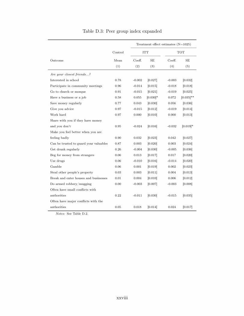
Table D.3: Peer group index expanded
Treatment effect estimates (N=1025)
Control ITT TOT
Outcome Mean Coeff. SE Coeff. SE
(1) (2) (3) (4) (5)
Are your closest friends...?
Interested in school 0.78 -0.002 [0.027] -0.003 [0.032]
Participate in community meetings 0.96 -0.014 [0.015] -0.018 [0.018]
Go to church or mosque 0.91 -0.015 [0.021] -0.019 [0.025]
Have a business or a job 0.58 0.055 [0.030]* 0.072 [0.035]**
Save money regularly 0.77 0.043 [0.030] 0.056 [0.036]
Give you advice 0.97 -0.015 [0.012] -0.019 [0.014]
Work hard 0.97 0.000 [0.010] 0.000 [0.013]
Share with you if they have money
and you don’t 0.95 -0.024 [0.016] -0.032 [0.019]*
Make you feel better when you are
feeling badly 0.90 0.032 [0.023] 0.042 [0.027]
Can be trusted to guard your valuables 0.87 0.003 [0.020] 0.003 [0.024]
Get drunk regularly 0.26 -0.004 [0.030] -0.005 [0.036]
Beg for money from strangers 0.06 0.013 [0.017] 0.017 [0.020]
Use drugs 0.06 -0.010 [0.016] -0.014 [0.020]
Gamble 0.06 0.001 [0.019] 0.002 [0.023]
Steal other people’s property 0.03 0.003 [0.011] 0.004 [0.013]
Break and enter houses and businesses 0.01 0.004 [0.010] 0.006 [0.012]
Do armed robbery/mugging 0.00 -0.003 [0.007] -0.003 [0.008]
Often have small conflicts with
authorities 0.22 -0.011 [0.030] -0.015 [0.035]
Often have major conflicts with the
authorities 0.05 0.018 [0.014] 0.024 [0.017]
Notes: See Table D.2.
xxviii
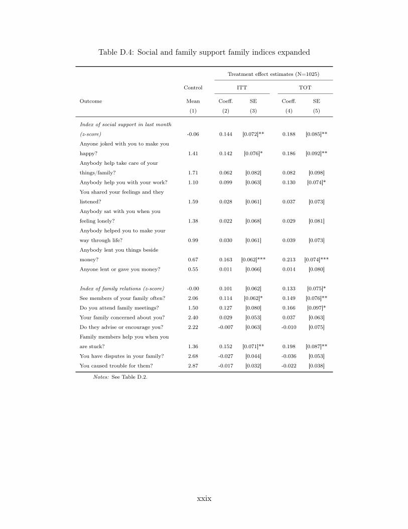
Table D.4: Social and family support family indices expanded
Treatment effect estimates (N=1025)
Control ITT TOT
Outcome Mean Coeff. SE Coeff. SE
(1) (2) (3) (4) (5)
Index of social support in last month
(z-score) -0.06 0.144 [0.072]** 0.188 [0.085]**
Anyone joked with you to make you
happy? 1.41 0.142 [0.076]* 0.186 [0.092]**
Anybody help take care of your
things/family? 1.71 0.062 [0.082] 0.082 [0.098]
Anybody help you with your work? 1.10 0.099 [0.063] 0.130 [0.074]*
You shared your feelings and they
listened? 1.59 0.028 [0.061] 0.037 [0.073]
Anybody sat with you when you
feeling lonely? 1.38 0.022 [0.068] 0.029 [0.081]
Anybody helped you to make your
way through life? 0.99 0.030 [0.061] 0.039 [0.073]
Anybody lent you things beside
money? 0.67 0.163 [0.062]*** 0.213 [0.074]***
Anyone lent or gave you money? 0.55 0.011 [0.066] 0.014 [0.080]
Index of family relations (z-score) -0.00 0.101 [0.062] 0.133 [0.075]*
See members of your family often? 2.06 0.114 [0.062]* 0.149 [0.076]**
Do you attend family meetings? 1.50 0.127 [0.080] 0.166 [0.097]*
Your family concerned about you? 2.40 0.029 [0.053] 0.037 [0.063]
Do they advise or encourage you? 2.22 -0.007 [0.063] -0.010 [0.075]
Family members help you when you
are stuck? 1.36 0.152 [0.071]** 0.198 [0.087]**
You have disputes in your family? 2.68 -0.027 [0.044] -0.036 [0.053]
You caused trouble for them? 2.87 -0.017 [0.032] -0.022 [0.038]
Notes: See Table D.2.
xxix
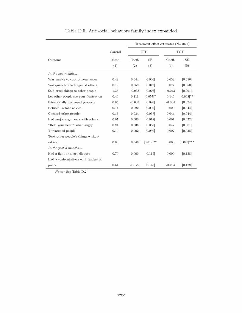
Table D.5: Antisocial behaviors family index expanded
Treatment effect estimates (N=1025)
Control ITT TOT
Outcome Mean Coeff. SE Coeff. SE
(1) (2) (3) (4) (5)
In the last month...
Was unable to control your anger 0.48 0.044 [0.046] 0.058 [0.056]
Was quick to react against others 0.19 0.059 [0.042] 0.077 [0.050]
Said cruel things to other people 1.36 -0.033 [0.076] -0.043 [0.091]
Let other people see your frustration 0.49 0.111 [0.057]* 0.146 [0.068]**
Intentionally destroyed property 0.05 -0.003 [0.020] -0.004 [0.024]
Refused to take advice 0.14 0.022 [0.036] 0.029 [0.044]
Cheated other people 0.13 0.034 [0.037] 0.044 [0.044]
Had major arguments with others 0.07 0.000 [0.018] 0.001 [0.022]
"Held your heart" when angry 0.94 0.036 [0.068] 0.047 [0.081]
Threatened people 0.10 0.002 [0.030] 0.002 [0.035]
Took other people’s things without
asking 0.03 0.046 [0.019]** 0.060 [0.023]***
In the past 6 months....
Had a fight or angry dispute 0.70 0.000 [0.115] 0.000 [0.138]
Had a confrontations with leaders or
police 0.64 -0.179 [0.148] -0.234 [0.178]
Notes: See Table D.2.
xxx
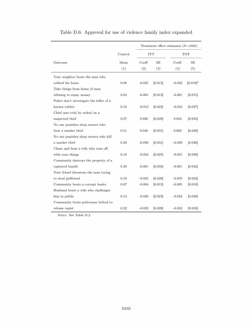
Table D.6: Approval for use of violence family index expanded
Treatment effect estimates (N=1025)
Control ITT TOT
Outcome Mean Coeff. SE Coeff. SE
(1) (2) (3) (4) (5)
Your neighbor beats the man who
robbed his home 0.08 -0.025 [0.015] -0.032 [0.018]*
Take things from home of man
refusing to repay money 0.04 -0.001 [0.013] -0.001 [0.015]
Police don’t investigate the killer of a
known robber 0.10 -0.012 [0.022] -0.016 [0.027]
Chief uses trial by ordeal on a
suspected thief 0.27 0.026 [0.029] 0.034 [0.035]
No one punishes shop owners who
beat a market thief 0.51 0.048 [0.031] 0.063 [0.038]
No one punishes shop owners who kill
a market thief 0.20 -0.030 [0.031] -0.039 [0.036]
Chase and beat a wife who runs off
with your things 0.19 -0.024 [0.025] -0.031 [0.030]
Community destroys the property of a
captured bandit 0.39 -0.001 [0.035] -0.001 [0.042]
Your friend threatens the man trying
to steal girlfriend 0.10 -0.025 [0.020] -0.033 [0.024]
Community beats a corrupt leader 0.07 -0.004 [0.015] -0.005 [0.019]
Husband beats a wife who challenges
him in public 0.14 -0.026 [0.023] -0.034 [0.028]
Community beats policeman bribed to
release rapist 0.22 -0.032 [0.028] -0.042 [0.033]
Notes: See Table D.2.
xxxi

Table D.7: Community participation family index expanded
Treatment effect estimates (N=1025)
Control ITT TOT
Outcome Mean Coeff. SE Coeff. SE
(1) (2) (3) (4) (5)
Number of groups involved in 5.36 0.288 [0.142]** 0.376 [0.168]**
Is a group leader 0.48 0.053 [0.033] 0.069 [0.039]*
Is a community leader 0.29 -0.019 [0.028] -0.024 [0.034]
Attended community meetings 0.94 -0.017 [0.020] -0.022 [0.025]
Believes can do things to improve
community 0.89 0.018 [0.018] 0.024 [0.021]
Volunteered for road clearing 0.78 0.007 [0.030] 0.009 [0.036]
Contributed to care of community
water sources 0.67 0.021 [0.036] 0.027 [0.043]
Contributed to other public facilities 0.63 0.010 [0.035] 0.013 [0.042]
Is a "big man" in community 0.35 0.003 [0.034] 0.004 [0.041]
Organizes new groups 0.50 0.009 [0.038] 0.011 [0.045]
People often come to you for advice 0.38 0.014 [0.033] 0.018 [0.039]
Community members come to you to
solve disputes 0.28 0.011 [0.033] 0.015 [0.039]
Your friends come to you to solve
disputes 0.83 0.011 [0.031] 0.014 [0.038]
Notes: See Table D.2.
xxxii
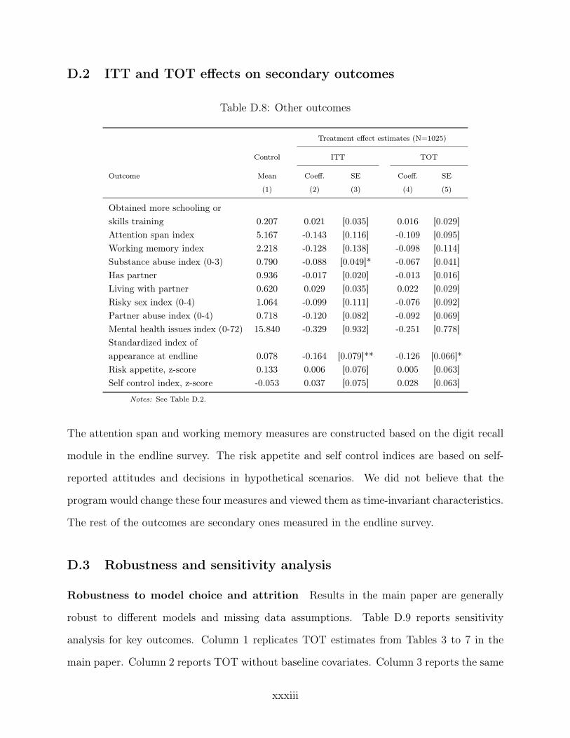
D.2 ITT and TOT effects on secondary outcomes
Table D.8: Other outcomes
Treatment effect estimates (N=1025)
Control ITT TOT
Outcome Mean Coeff. SE Coeff. SE
(1) (2) (3) (4) (5)
Obtained more schooling orskills training 0.207 0.021 [0.035] 0.016 [0.029]Attention span index 5.167 -0.143 [0.116] -0.109 [0.095]Working memory index 2.218 -0.128 [0.138] -0.098 [0.114]Substance abuse index (0-3) 0.790 -0.088 [0.049]* -0.067 [0.041]Has partner 0.936 -0.017 [0.020] -0.013 [0.016]Living with partner 0.620 0.029 [0.035] 0.022 [0.029]Risky sex index (0-4) 1.064 -0.099 [0.111] -0.076 [0.092]Partner abuse index (0-4) 0.718 -0.120 [0.082] -0.092 [0.069]Mental health issues index (0-72) 15.840 -0.329 [0.932] -0.251 [0.778]Standardized index ofappearance at endline 0.078 -0.164 [0.079]** -0.126 [0.066]*Risk appetite, z-score 0.133 0.006 [0.076] 0.005 [0.063]Self control index, z-score -0.053 0.037 [0.075] 0.028 [0.063]
Notes: See Table D.2.
The attention span and working memory measures are constructed based on the digit recall
module in the endline survey. The risk appetite and self control indices are based on self-
reported attitudes and decisions in hypothetical scenarios. We did not believe that the
program would change these four measures and viewed them as time-invariant characteristics.
The rest of the outcomes are secondary ones measured in the endline survey.
D.3 Robustness and sensitivity analysis
Robustness to model choice and attrition Results in the main paper are generally
robust to different models and missing data assumptions. Table D.9 reports sensitivity
analysis for key outcomes. Column 1 replicates TOT estimates from Tables 3 to 7 in the
main paper. Column 2 reports TOT without baseline covariates. Column 3 reports the same
xxxiii

TOT estimates as in Column 1 but without clustering at the village level. Column 4 uses
an alternate instrument for assignment to treatment—instead of counting the first m men in
each block as assigned to treatment up until the that block’s quota b is filled (so that m ≥ b),
the results in Column 4 do not count the m > b men as assigned to treatment (rather, they
are non-compliant).42
In general the qualitative conclusions are the same. Omitting covariates or using the
alternate instrument slightly reduces the statistical significance of some effects, as one would
expect.
Columns 5 to 7 consider whether our treatment effects could be the result of selective
attrition. We estimate bounds by imputing outcome values for unfound individuals at differ-
ent points of the observed outcome distribution, focusing on the cases that reduce program
impacts. For positive outcomes we impute the observed mean plus x standard deviations of
the distribution for the control group, and for the treatment group we impute the observed
treatment mean minus x standard deviations of the distribution. We calculate estimates for
x = 0.1, 0.25, and 0.5. Note these imply large systematic differences between the missing
treatment and control members. All treatment effects in are robust to x = 0.1 and the
majority are still robust to x = 0.25. The sign on treatment is preserved when x = 0.5.
Robustness of mercenary recruitment index We also consider permutations of the
mercenary recruitment index in Table D.10. The table shows that the TOT estimate on the
full index is robust to excluding various components, or to including an indictor for being
physically found by our survey at endline in a border area (which is rare). The statistical
significance of the treatment effect falls if we exclude all indirect proxies and “talked to a
commander” but still has a similar sign and magnitude.42This increases noise and estimates a different local average treatment effect than in Column (1), but
avoids the small risk that the marginal person selected into treatment assignment in each is endogenously amore compliant type. The quota was usually 50% of the men registered in the block, whereas on average 57%were assigned to treatment using our ordered assignment method. Ideally we would use this 57% average asthe instrument, counting people as assigned if they were in the first 57% of the block order, but we do nothave the historical ranking in every block to do so.
xxxiv
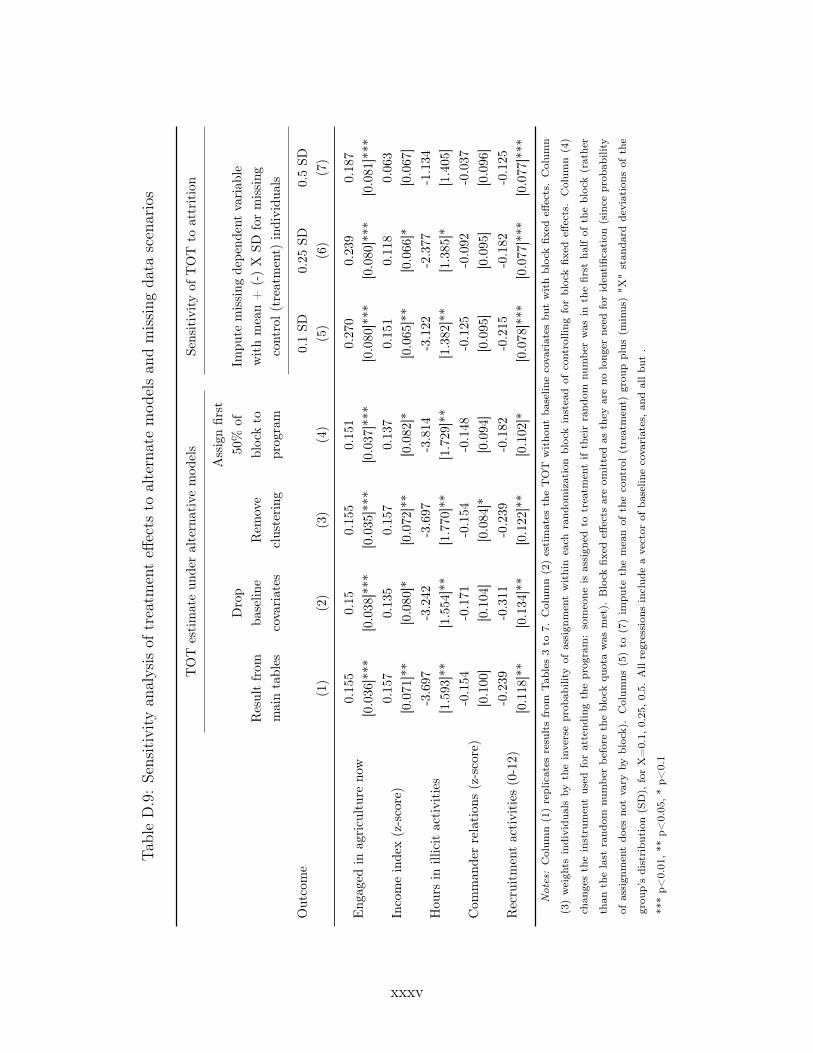
T ableD.9:Sensitivity
analysis
oftreatm
enteff
ects
toalternatemod
elsan
dmissing
data
scenarios
TOT
estimateun
deralternativemod
els
Sensitivityof
TOT
toattrition
Resultfrom
maintables
Drop
baselin
ecovariates
Rem
ove
clustering
Assignfirst
50%
ofblockto
program
Impu
temissing
depe
ndentvariab
lewithmean+
(-)X
SDformissing
control(treatm
ent)
individu
als
Outcome
0.1SD
0.25
SD0.5SD
(1)
(2)
(3)
(4)
(5)
(6)
(7)
Eng
aged
inagricultureno
w0.155
0.15
0.155
0.151
0.27
00.23
90.18
7[0.036]***
[0.038]***
[0.035]***
[0.037]***
[0.080
]***
[0.080
]***
[0.081
]***
Incomeinde
x(z-score)
0.157
0.135
0.157
0.137
0.15
10.11
80.06
3[0.071]**
[0.080]*
[0.072]**
[0.082]*
[0.065
]**
[0.066
]*[0.067
]
Hou
rsin
illicitactivities
-3.697
-3.242
-3.697
-3.814
-3.122
-2.377
-1.134
[1.593]**
[1.554]**
[1.770]**
[1.729]**
[1.382
]**
[1.385
]*[1.405
]
Com
man
derrelation
s(z-score)
-0.154
-0.171
-0.154
-0.148
-0.125
-0.092
-0.037
[0.100]
[0.104]
[0.084]*
[0.094]
[0.095
][0.095
][0.096
]
Recruitmentactivities
(0-12)
-0.239
-0.311
-0.239
-0.182
-0.215
-0.182
-0.125
[0.118]**
[0.134]**
[0.122]**
[0.102]*
[0.078
]***
[0.077
]***
[0.077
]***
Not
es:Colum
n(1)replicates
resultsfrom
Tab
les3to
7.Colum
n(2)estimates
theTOT
witho
utba
selin
ecovariates
butwithblockfix
edeff
ects.Colum
n
(3)weigh
tsindividu
alsby
theinverseprob
ability
ofassign
mentwithineach
rand
omizationblockinsteadof
controlling
forblockfix
edeff
ects.Colum
n(4)
chan
gestheinstrumentused
forattend
ingtheprogram:someone
isassign
edto
treatm
entiftheirrand
omnu
mbe
rwas
inthefirst
halfof
theblock(rather
than
thelast
rand
omnu
mbe
rbe
fore
theblockqu
otawas
met).
Block
fixed
effects
areom
ittedas
they
areno
long
erneed
foridentification(since
prob
ability
ofassign
mentdo
esno
tvary
byblock).Colum
ns(5)to
(7)im
pute
themeanof
thecontrol(treatment)
grou
pplus
(minus)"X
"stan
dard
deviations
ofthe
grou
p’sdistribu
tion
(SD),forX=0.1,
0.25,0.5.
Allregression
sinclud
eavector
ofba
selin
ecovariates,an
dallbu
t.
***p<
0.01,**
p<0.05,*p<
0.1
xxxv

Table D.10: Program impacts on mercenary recruitment proxies
Control TOT estimate
Outcome Mean Coeff. SE(1) (2) (3)
All recruitment interest/actions (0-16) 2.41 -0.397 [0.154]***All, excluding "talked to a commander" (0-15) 1.97 -0.289 [0.145]**All, excluding "partisan preference" (0-15) 2.86 -0.506 [0.173]***All, excluding "talked to a commander" and "partisan preference (0-14) 2.41 -0.397 [0.154]***
Direct only (0-12) 0.94 -0.239 [0.118]**Direct only, including "found in border town at endline" (0-13) 0.94 -0.233 [0.117]**
Found in border town at endline 0.00 0.007 [0.006]Direct only, excluding "talked to a commander" (0-11) 0.49 -0.131 [0.103]Direct only, excluding "would go to CI for $1000" (0-11) 0.86 -0.198 [0.109]*
Notes: Columns (2)-(3) report the the effect of treatment on the treated (TOT) via two-stage least squares.
Regressions include block dummies and baseline covariates. Standard errors are clustered at the village level. See
Appendix D.1 for ITT results.
*** p<0.01, ** p<0.05, * p<0.1
Robustness of package choice estimates The estimates of the impact of in-kind inputs
in Section 6.3 require an assumption of selection on observables (conditional unconfound-
edness). We examine the sensitivity of our estimates to violations of this assumption using
a technique proposed by Guido Imbens.43 We illustrate the sensitivity in Figure D.1 for
two dependent variables: the index of mercenary recruitment interest and actions, and the
hours per week of illicit work. Any unobserved confounder must be correlated with both
the dependent variable and treatment assignment (in this case, the choice of animals as a
package). The curve in each figure represents all combinations of correlation between an
unobservable variable and the outcome (vertical axis) and animal choice (horizontal axis)
that would reduce the observed treatment effect by half. The axes represent the hypotheti-
cal increase in partial R-squared that would result from observing this unobserved covariate
and including it in a regression with either the outcome or the treatment as the dependent
variable. The curve represents a threshold. Any covariate that laid to the right of the curve43Imbens, Guido W., "Sensitivity to Exogeneity Assumptions in Program Evaluation", The American
Economic Review 93 (2003), pp. 126–32. 2
xxxvi

would indicate that our conditional unconfoundedness assumption is highly suspect.
How do we know where the unobservables lie? We do not, of course, but we can bench-
mark them against observed covariates. The + signs indicate the partial R-squared added
by our observed covariates. We focus on only a handful of key covariates, and test classes
of covariates (e.g. all economic performance measures) since dropping just one of a large
class (e.g. income but not assets and work hours) would by construction have a low partial
R-squared. The covariates include region fixed effect.
We see that entire classes of covariates, such as regional covariates or all economic or all
social variables, have little influence on our treatment effects. For an unobserved covariate
to bias our results, it must be wholly unlike other covariates we observe. We judge this to
be unlikely given the richness of our data.
xxxvii
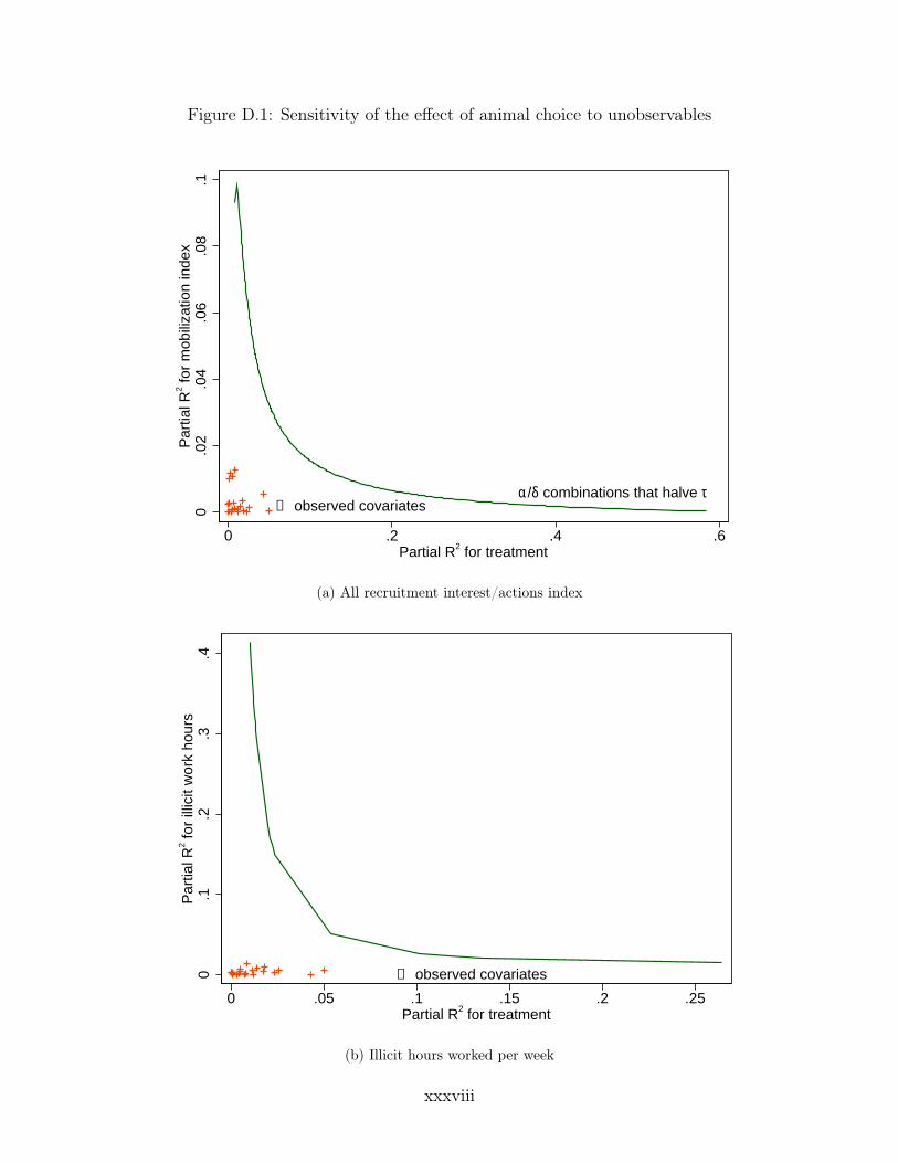
Figure D.1: Sensitivity of the effect of animal choice to unobservables
a/d combinations that halve t¬ observed covariates0
.02
.04
.06
.08
.1P
artia
l R2 fo
r m
obili
zatio
n in
dex
0 .2 .4 .6Partial R2 for treatment
(a) All recruitment interest/actions index
a/d combinations that halve t¬ observed covariates0
.1.2
.3.4
Par
tial R
2 for
illic
it w
ork
hour
s
0 .05 .1 .15 .2 .25Partial R2 for treatment
(b) Illicit hours worked per week
xxxviii
D.4 Heterogeneity by group affiliation/identity
As discussed in Section 6.3, the Krahn ethnic group was believed to be closely aligned with
Gbagbo’s side in the Ivoirian war. Indeed, in an OLS regression of support for Gbagbo
on Krahn ethnicity and all other baseline covariates, Krahns are 34 percentage points more
likely to support Gbagbo (regressions not shown). This is not the case for other groups in the
Kru language family, or for ex-fighters from the Liberian armed group MODEL, which had
support from Gbagbo. Similarly, we see no groups that report systematically higher support
for Ouattara’s side in the conflict, including Liberian Muslims and former members of the
ethnically-Muslim rebel group ULIMO-K. Hence Krahn identity, though there are only 21
in our sample, is a string indicator of solidarity with Gbagbo.
In Table D.11 we interact Krahn identity with treatment and examine the effects on
illicit hours and recruitment activities. We can see that the Krahn identity (the coefficient
on the indicator alone) is associated with 4.1 more illicit hours per week and a one standard
deviation increase in recruitment interest and action according to our index of proxies. The
overall treatment effects are preserved in the full sample, though they are slightly smaller
in magnitude. The coefficient on the interaction between treatment and Krahn, however, is
large and negative. It effectively cancels out the heightened effect of simply being Krahn,
and then some. That is, the treatment appears to neutralize the elevated levels of insecurity
among Krahns especially.
xxxix

Table D.11: Heterogeneity by ethnic affiliation to armed groups
Dependent variable
Covariate Hours per week in
illicit activities
All recruitment
interest/actions,
z-score
(1) (2)
Assigned to treatment -2.995 -0.135
[1.422]** [.063]**
Assigned to treatment " Krahn ethnicity -17.413 -1.131
[9.000]* [.585]*
Krahn ethnicity 4.104 1.045
[6.847] [.520]**
Mean of dependent variable, control group 15.57 0.09
Notes: The table displays OLS regressions of the dependent variable on the listed covariates plus
all other baseline covariates and strata fixed effects (not displayed). Standard errors clustered at the
community level.
*** p<0.01, ** p<0.05, * p<0.1
xl
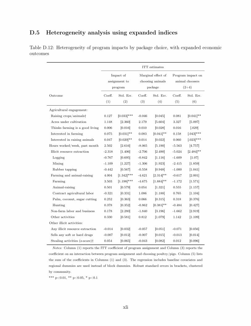
D.5 Heterogeneity analysis using expanded indices
Table D.12: Heterogeneity of program impacts by package choice, with expanded economicoutcomes
ITT estimates
Impact of
assignment to
program
Marginal effect of
choosing animals
package
Program impact on
animal choosers
(2+4)
Outcome Coeff. Std. Err. Coeff. Std. Err. Coeff. Std. Err.
(1) (2) (3) (4) (5) (6)
Agricultural engagement:
Raising crops/animals† 0.127 [0.033]*** -0.046 [0.045] 0.081 [0.041]**
Acres under cultivation 1.148 [2.360] 2.179 [5.604] 3.327 [5.097]
Thinks farming is a good living 0.006 [0.016] 0.010 [0.028] 0.016 [.029]
Interested in farming 0.075 [0.031]** 0.083 [0.041]** 0.158 [.043]***
Interested in raising animals 0.047 [0.020]** 0.014 [0.022] 0.060 [.023]***
Hours worked/week, past month 2.502 [2.616] -8.065 [5.190] -5.563 [4.757]
Illicit resource extraction -2.318 [1.406] -2.706 [2.490] -5.024 [2.484]**
Logging -0.767 [0.695] -0.842 [1.116] -1.609 [1.07]
Mining -1.109 [1.227] -1.306 [1.923] -2.415 [1.859]
Rubber tapping -0.442 [0.567] -0.558 [0.948] -1.000 [1.041]
Farming and animal-raising 4.004 [1.342]*** -4.621 [2.314]** -0.617 [2.001]
Farming 3.503 [1.198]*** -4.675 [1.884]** -1.172 [1.571]
Animal-raising 0.501 [0.579] 0.054 [1.321] 0.555 [1.157]
Contract agricultural labor -0.321 [0.331] 1.086 [1.188] 0.765 [1.104]
Palm, coconut, sugar cutting 0.252 [0.363] 0.066 [0.315] 0.318 [0.376]
Hunting 0.378 [0.352] -0.862 [0.381]** -0.484 [0.427]
Non-farm labor and business 0.178 [2.280] -1.840 [3.196] -1.662 [2.919]
Other activities 0.330 [0.581] 0.812 [1.079] 1.142 [1.109]
Other illicit activities:
Any illicit resource extraction -0.014 [0.032] -0.057 [0.051] -0.071 [0.056]
Sells any soft or hard drugs -0.007 [0.012] -0.007 [0.015] -0.013 [0.014]
Stealing activities (z-score)† 0.054 [0.065] -0.043 [0.082] 0.012 [0.096]
Notes: Column (1) reports the ITT coefficient of program assignment and Column (3) reports the
coefficient on an interaction between program assignment and choosing poultry/pigs. Column (5) lists
the sum of the coefficients in Columns (1) and (3). The regression includes baseline covariates and
regional dummies are used instead of block dummies. Robust standard errors in brackets, clustered
by community.
*** p<0.01, ** p<0.05, * p<0.1
xli
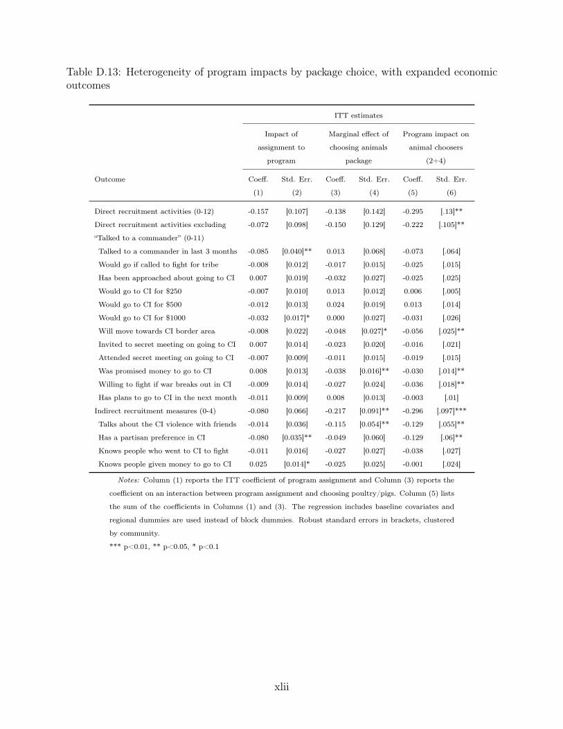
Table D.13: Heterogeneity of program impacts by package choice, with expanded economicoutcomes
ITT estimates
Impact of
assignment to
program
Marginal effect of
choosing animals
package
Program impact on
animal choosers
(2+4)
Outcome Coeff. Std. Err. Coeff. Std. Err. Coeff. Std. Err.
(1) (2) (3) (4) (5) (6)
Direct recruitment activities (0-12) -0.157 [0.107] -0.138 [0.142] -0.295 [.13]**
Direct recruitment activities excluding
“Talked to a commander” (0-11)
-0.072 [0.098] -0.150 [0.129] -0.222 [.105]**
Talked to a commander in last 3 months -0.085 [0.040]** 0.013 [0.068] -0.073 [.064]
Would go if called to fight for tribe -0.008 [0.012] -0.017 [0.015] -0.025 [.015]
Has been approached about going to CI 0.007 [0.019] -0.032 [0.027] -0.025 [.025]
Would go to CI for $250 -0.007 [0.010] 0.013 [0.012] 0.006 [.005]
Would go to CI for $500 -0.012 [0.013] 0.024 [0.019] 0.013 [.014]
Would go to CI for $1000 -0.032 [0.017]* 0.000 [0.027] -0.031 [.026]
Will move towards CI border area -0.008 [0.022] -0.048 [0.027]* -0.056 [.025]**
Invited to secret meeting on going to CI 0.007 [0.014] -0.023 [0.020] -0.016 [.021]
Attended secret meeting on going to CI -0.007 [0.009] -0.011 [0.015] -0.019 [.015]
Was promised money to go to CI 0.008 [0.013] -0.038 [0.016]** -0.030 [.014]**
Willing to fight if war breaks out in CI -0.009 [0.014] -0.027 [0.024] -0.036 [.018]**
Has plans to go to CI in the next month -0.011 [0.009] 0.008 [0.013] -0.003 [.01]
Indirect recruitment measures (0-4) -0.080 [0.066] -0.217 [0.091]** -0.296 [.097]***
Talks about the CI violence with friends -0.014 [0.036] -0.115 [0.054]** -0.129 [.055]**
Has a partisan preference in CI -0.080 [0.035]** -0.049 [0.060] -0.129 [.06]**
Knows people who went to CI to fight -0.011 [0.016] -0.027 [0.027] -0.038 [.027]
Knows people given money to go to CI 0.025 [0.014]* -0.025 [0.025] -0.001 [.024]
Notes: Column (1) reports the ITT coefficient of program assignment and Column (3) reports the
coefficient on an interaction between program assignment and choosing poultry/pigs. Column (5) lists
the sum of the coefficients in Columns (1) and (3). The regression includes baseline covariates and
regional dummies are used instead of block dummies. Robust standard errors in brackets, clustered
by community.
*** p<0.01, ** p<0.05, * p<0.1
xlii