camera calibration with distortion models and accuracy ... · model. in the second step, the...

IEEE TRANSACTIONS ON P A m R N ANALYSIS AND MACHINE INTELLIGENCE, VOL. 14, NO. 10, OCTOBER 1992 965

Camera Calibration with Distortion Models and Accuracy Evaluation

Juyang Weng, Member, IEEE, Paul Cohen, and Marc Herniou

Abstract- The objective of stereo camera calibration is to estimate the internal and external parameters of each camera. Using these parameters, the 3-D position of a point in the scene, which is identified and matched in two stereo images, can be determined by the method of triangulation. In this paper, we present a camera model that accounts for major sources of camera distortion, namely, radial, decentering, and thin prism distortions. The proposed calibration procedure consists of two steps. In the first step, the calibration parameters are estimated using a closed-form solution based on a distortion-free camera model. In the second step, the parameters estimated in the first step are improved iteratively through a nonlinear optimization, taking into account camera distortions. According to minimum variance estimation, the objective function to be minimized is the mean-square discrepancy between the observed image points and their inferred image projections computed with the estimated calibration parameters. We introduce a type of measure that can be used to directly evaluate the performance of calibration and compare calibrations among different systems. The validity and performance of our calibration procedure are tested with both synthetic data and real images taken by tele- and wide-angle lenses. The results consistently show significant improvements over less complete camera models.

Index Terms- Camera calibration, lens distortion, optimization. stereo.

I. INTRODUCTION ALIBRATION OF cameras is considered as an important C issue in computer vision. Accurate calibration of cameras

is especially crucial for applications that involve quantitative measurements such as dimensional measurements, depth from stereoscopy, or motion from images.

One aspect of camera calibration is to estimate the internal parameters of the camera. These parameters determine how the image coordinates of a point are derived, given the spatial position of the point with respect to the camera. The estimation of the geometrical relation between the camera and the scene, or between different cameras, is also an important aspect of calibration. The corresponding parameters that characterize such a geometrical relation are called external parameters. It is well known that actual cameras are not perfect and

Manuscript received January 18, 1990; revised February 24, 1992. This research was supported by the Natural Sciences and Engineering Council of Canada under Grant A3890 and grants from Centre de Recherche Informa- tique de Montreal and Ecole Polytechnique de Montreal. Recommended for acceptance by Associate Editor J . Mundy.

J. Weng is with the Department of Computer Science, Michigan State University, East Lansing, MI 48824-1027.

P. Cohen and M. Hemiou are with the Department of Electrical Engineering, Ecole Polytechnique de Montreal, Montreal, Canada H3C 3A7.

IEEE Log Number 9201774.

sustain a variety of aberrations. For geometrical measurements, the main concern is camera distortion, which relates to the position of image points in the image plane but not directly to the image quality. For example, the position of a point in a slightly blurred image can still be measured as the center of the blurred point. However, if the image position of a point is not accurate, the results that depend on its image coordinates will be erroneous.

Camera calibration has long been an important issue in the photogrammetry community. With the increasing need for higher accuracy measurement in computer vision, it has also attracted research efforts in the computer vision community. Compared with the high-quality metric cameras used in photogrammetry, the cameras commonly used in computer vision have the following characteristics: a) Image spatial resolution is defined by spatial digitization and is relatively low (e.g., a typical CCD sensing array has about 512 x 480 pixels); b) lenses used for video cameras are nonmetric off-the-shelf lenses and sustain a substantial amount of distortion; c) camera assembly sustains considerable internal misalignment (e.g., the CCD sensing array may not be orthogonal to the optical axis, and the center of the array may not coincide with the optical principal point, i.e., the intersection of the optical axis and the image plane).

The existing techniques for camera calibration can be clas- sified into the following categories.

1) Direct Nonlinear Minimization: In this category, equations that relate the parameters to be estimated with the 3-D coordinates of control points and their image plane projections are established. The search for the parameters involves using an iterative algorithm with the objective of minimizing residual errors of some equations. Most of the classical calibration techniques in photogrammetry belong to this category (e.g., [3], [l], [15], [4], [ll]). One advantage of this type of technique is that the camera model can be very general to cover many types of distortion. Some simple distortion-free models for computer vision applications have also employed this type of technique (e.g., [7], [9]). Another advantage is that the algorithm may achieve high accuracy, provided that the estimation model is good, and correct convergence has been reached. However, since the algorithm is iterative, the procedure may end up with a bad solution unless a good initial guess is available. Furthermore, once distortion parameters are included in the parameter space, the minimization may be unstable if the procedure of iterations is not properly designed. The interaction between the distortion parameters and external parameters can lead to divergence or false solutions.

0162-8828/92$03.00 0 1992 IEEE

Authorized licensed use limited to: The University of Auckland. Downloaded on March 17,2010 at 06:35:02 EDT from IEEE Xplore. Restrictions apply.

966 IEEE TRANSACTIONS ON P A m R N ANALYSIS AND MACHINE INTELLIGENCE, VOL. 14, NO. 10, OCTOBER 1992

2) Closed-Form Solution: With this type of scheme, parameter values are computed directly through a noniterative algorithm based on a closed-form solution (e.g., [l] , [15], [8], [6]). A set of intermediate parameters is defined in terms of the original parameters. The intermediate parameters can be computed by solving linear equations, and the final parameters are determined from those intermediate parameters. Since no iteration is required, the algorithms are fast. However, such methods have the following disadvantages. First, camera distortion cannot be incorporated, and therefore, distortion effects cannot be corrected. It is worth mentioning that the direct linear transformation (DLT) introduced by Abdel-Aziz and Karara [ l ] has been extended to incorporate distortion parameters. However, the corresponding formulation is not exact; depth components of control points, in a camera-centered coordinate system, are assumed to be constant. Second, due to the objective to construct a noniterative algorithm, the actual constraints in the intermediate parameters are not considered. Consequently, in the presence of noise, the intermediate solution does not satisfy the constraints, and the accuracy of the final solution is relatively poor.

3) Two-step Methods: The methods of this type involve a direct solution for most of the calibration parameters and some iterative solution for the other parameters. The existing techniques include those presented by Tsai [13] and Lenz and Tsai [lo]. A radial alignment constraint is used to derive a closed-form solution for the external parameters and the effective focal length of the camera. Then, an iterative scheme is used to estimate three parameters: the depth component in the translation vector (external parameter), the effective focal length, and a radial distortion coefficient. In [lo], two additional parameters (the image coordinates of the principal point, which were considered to be known in [13]) have been included into the set of iteratively determined parameters. The advantages of their method are as follows: a) A closed-form solution is derived for most of the parameters; b) the closed- form solution is immune to lens radial distortion; c) the number of parameters to be estimated through iterations is relatively small. The disadvantages are as follows: a) Their method can only handle radial distortion and cannot be extended to other types of distortion; b) the solution is not optimal because the information provided by the calibration points has not been fully utilized. The radial component of a point is discarded completely, and only the tangential component is used for the solution. However, although it is generally true that the radial component is less reliable than the tangential component, the tangential component is not error free either. From a statistical point of view, discarding relatively unreliable radial components (which account for half of the observations) results in a less reliable estimator.

In this paper, we address the above problems and introduce our approach to camera calibration.

1) For the calibration of off-the-shelf nonmetric cameras, we derive a model that takes into account major distortions and investigate the amount of penalty caused by less general camera models. This will allow us to address important questions such as the following:

Is it at all necessary to consider distortion for popular

off-the-shelf video cameras with, for instance, a typical 512 x 512 image resolution? How much improvement is brought about by considering one or several types of distortion phenomena in the model?

It was reported in [6] that triangulation with an accuracy of one in 2000 parts had been achieved by calibration based on a distortion-free model. A comparable result was reported in [13] with a simple one-parameter radial distortion model and no consideration of tangential distortion. In Faig’s very elaborate model [4], four types of distortion were considered for high-accuracy photogrammetric applications: radial symmetric distortion, decentering distortion, affinity distortion, and distortion caused by nonperpendicularity of axis. We will find some answers to the above questions in our experiments with three different models: the distortion-free model, the radial distortion model, and our complete model that includes both radial and tangential distortions.

2 ) We adopt a two-step approach to the calibration of our stereo camera system. The first-step consists of using a noniterative algorithm to directly compute a closed-form solution for all the external parameters and some major internal parameters based on a distortion-free camera model. The second step is a nonlinear optimization based on a camera model that incorporates distortion using the solution of the first step as an initial guess. One major difference between our two-step computational approach and those of [13] and [lo] is that our second step is an optimization that computes and improves all the parameters, whereas in the approaches of [13] and [lo], the second step iteratively computes only a few parameters that cannot be provided by the first step. Our approach was motivated by the following considerations: a) Since the algorithm that computes a closed-form solution is noniterative, it is fast, and a solution is generally guaranteed. It gives a complete solution to all external and internal parameters of a distortion-free camera model. Since the center of an image has little distortion, only the points near the center of the image (which are called central points) are used for the closed-form solution. Consequently, the closed-form solution is not affected very much by distortion and is good enough to be used as an initial guess for further optimization. b) The nonlinear optimization step can take into account different types of distortion. c) Even if the actual camera is distortion free, nonlinear optimization can still improve the closed-form solution. Indeed, the closed-form solution is usually the solution that minimizes mean-square residuals of some equations. However, because various uncertainties in the different equations have not been properly taken into account, the solution is not optimal. The optimization step will then compute the “best” solution. d) In general, a nonlinear optimization algorithm may converge to a local extremum that is not globally optimal. However, if an approximate solution is given as an initial guess, the number of iterations can be significantly reduced, and the globally optimal solution can be reliably reached. Such a two-step algorithm is much more reliable than a direct iterative algorithm that starts with an arbitrarily chosen initial guess (e.g., “zero” guess). e) Real- time calibration is not necessary in most applications. Usually,


967 WENG et al.: CAMERA CALIBRATION WITH DISTORTION MODELS

calibration needs to be done only once, and the estimated parameters are used for real-time operation. This is also true for time-varying systems in which the calibrated camera parameters are given as functions of camera control signals. Therefore, the calibration algorithm can use considerable time to obtain highly accurate parameters.

3) We introduce a new measure to assess the accuracy of camera calibration with digital images. The existing measures depend on the setup of the system, especially on the field of view, the baseline length, and the camera-to-object distance. This makes it very difficult to compare techniques of calibrations with different setups. As we know, image resolution inherently limits the accuracy of calibration. The calibrated parameters cannot be exact even if the camera is ideal. However, a good calibration with a lower image resolution may exceed the accuracy of a poor calibration with a higher resolution. It is reasonable to measure the quality of calibration based on image resolution. The measure introduced in this paper is called normalized stereo camera error, which is an error measure normalized according to the resolution of the images. Such a normalized measure is important because a) the performance of different calibration approaches can be quantitatively evaluated and compared, and b) this measure indicates whether a particular camera model is elaborate enough under the image resolution. Since the resolution of a digital image is well defined by the number of pixels, this measure is especially convenient for calibrations that are based on digital images.

We present our camera models in the next section. The estimation of the parameters is discussed in Section 111. In Section IV, we introduce the normalized stereo camera error. The performance of our method is demonstrated by the results of simulations and experiments with real camera systems in Section V. Finally, Section VI gives concluding remarks.

0 Ey /" xc

t t

0, I/ Yc

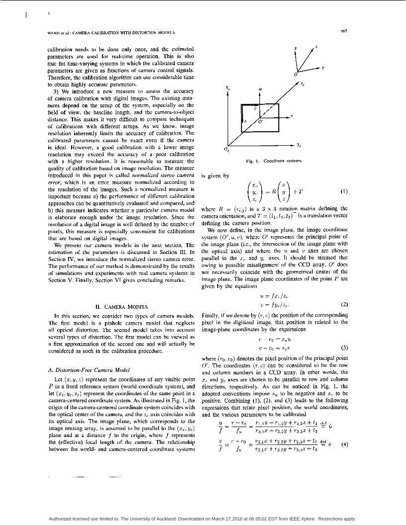
Fig. 1 . Coordinate systems.

is given by

where R = (r i , j ) is a 3 x 3 rotation matrix defining the camera orientation, and T = (t l , t z , t ~ ) ~ is a translation vector defining the camera position.

We now define, in the image plane, the image coordinate system (0', U , U), where 0' represents the principal point of the image plane (i.e., the intersection of the image plane with the optical axis) and where the U and ZI axes are chosen parallel to the 2, and yc axes. It should be stressed that owing to possible misalignment of the CCD array, 0' does not necessarily coincide with the geometrical center of the image plane. The image plane coordinates of the point P are given by the equations

U = f x c l z ,

11. CAMERA MODELS = fYc /Zc . (2 )

In this section, we consider two types of camera models. The first model is a pinhole camera model that neglects all optical distortion. The second model takes into account several types of distortion. The first model can be viewed as a first approximation of the second one and will actually be considered as such in the calibration procedure.

A. Distortion-Free Camera Model

Let (x, y, z ) represent the coordinates of any visible point P in a fixed reference system (world coordinate system), and let (xc, yc, z,) represent the coordinates of the same point in a camera-centered coordinate system. As illustrated in Fig. 1, the origin of the camera-centered coordinate system coincides with the optical center of the camera, and the z , axis coincides with its optical axis. The image plane, which corresponds to the image sensing array, is assumed to be parallel to the (x,, y,) plane and at a distance f to the origin, where f represents the (effective) focal length of the camera. The relationship between the world- and camera-centered coordinate systems

Finally, if we denote by ( T , e ) the position of the corresponding pixel in the digitized image, this position is related to the image-plane coordinates by the expressions

T - To = suu c - CO = s v v

where ( T O , C O ) denotes the pixel position of the principal point 0'. The coordinates ( T , c ) can be considered to be the row and column numbers in a CCD array. In other words, the x, and yc axes are chosen to be parallel to row and column directions, respectively. As can be noticed in Fig. 1, the adopted conventions impose s, to be negative and sv to be positive. Combining (l), (2), and (3) leads to the following expressions that relate pixel position, the world coordinates, and the various parameters to be calibrated

(3)

- - 'U - - T - TO - - T l , l ~ + T l , Z y + T 1 , 3 Z + t l kf - .iL f f u T 3 , l x + T3,Zy + T3,3Z + t 3

(4) - c - CO - - T Z J ~ + rz,zy + T2,3Z + t z g ir - - -

f fv T 3 , l x -k T3,ZY + T3,3z + t3


968 IEEE TRANSACTIONS ON PATTERN ANALYSIS AND MACHINE INTELLIGENCE, VOL. 14, NO. 10, OCTOBER 1992

where (iL,ir) defines the coordinates in the normalized image plane that is located at z = 1, and f, = s,f and f , = s,f are called row focal length and column focal length, respectively. If we scale the camera, with respect to the focal point, so that the row-to-row (column-to-column) pixel spacing is equal to 1, the corresponding focal length of such a scaled camera is equal to the row (column) focal length. Most conventional cameras produce rectangular images with a ratio of about 4/3 between horizontal and vertical dimensions. If the ratio of row-to-row pixel distances to column-to-column distance is q, the ratio If,/fvl is roughly equal to 4- l . However, because of the timing errors, unstability of the scanning electronics, and a possible tilt of the CCD array, the ratio If,/fvl is not exactly q - l , although q can be directly computed from

dr: tangential distortion

the dimensional specifications of the CCD sensing elements provided by camera manufacturers.

With this camera model, the calibration txoblem is ex- Fig. 2. Radial and tangential distortions.

/ A I

I ---____--dC

pressed in the following terms: t-<-- \

Given a sufficient number of visible points whose world \I

coordinates (xi, y;, z i ) are known with a high precision, as well as their corresponding observed pixel positions (T : , ct), estimate, in some optimal sense, the value of the internal camera parameters T O , co, f u , f , and the external parameters R and T. In general, observed pixel locations ( ( , c : ) are not equal to locations ( ~ i , c i ) resulting from (4) because of acquisition and spatial digitization noise and point extraction

I

\ I I I I I I I I I I

I I I I I I I I I I

- \

B. Geometrical Distortion

in the image plane. As a result of several types of imperfections

Fig. 3. Effect of radial distortion. Solid lines: no distortion; dashed lines: Geometrical distortion concerns the position of image points with radial distortion (a: negative, b: positive).

in the design and Optical system, the expressions in (2) do not

Of lenses the and the scale to decrease. A positive radial displacement is referred to as pincushion distortion. It causes outer points to and must

be replaced by expressions that explicitly take into account the positional error thus introduced:

spread and the scale to increase. This type of distortion is strictly symmetric about the optical axis. Fig. 3 illustrates the

U’ = U + & ( U , U)

U’ = U + & ( U , U)

effect of radial distortion.

by an expression of the following form [ l l ] , [4]: The radial distortion of a perfectly centered lens is governed

( 5 )

where U and U are the nonobservable, distortion-free image coordinates, and U’ and U‘ are the corresponding coordinates with distortion. As indicated by (9, the amount of positional error along each coordinate usually depends on the point position. In order to correct distortion, we need to analyze various sources of distortion and model their effects in the image plane.

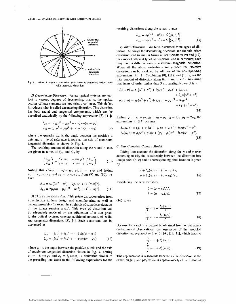
In this paper, we consider three types of distortion. The first one is caused by imperfect lens shape and manifests itself by radial positional error only, whereas the second and the third types of distortion are generally caused by improper lens and camera assembly and generate both radial and tangential errors in point positions (see Fig. 2).

1) Radial Distortion: Radial distortion causes an inward or outward displacement of a given image point from its ideal location. This type of distortion is mainly caused by flawed radial curvature curve of the lens elements. A negative radial displacement of the image points is referred to as barrel distortion. It causes outer points to crowd increasingly together

where p is the radial distance from the principal point of the image plane, and k l , Icz, k3,. . . are the coefficients of radial distortion. At each image point represented by polar coordinates (p , cp), radial distortion corresponds to the distortion along radial (p) direction. The image point can also be expressed in terms of the Cartesian coordinates ( U , U ) with

U = pcoscp

U = psincp (7)

and the amount of distortion along each of the Cartesian image coordinates can be represented by


WENG et al.: CAMERA CALIBRATION WITH DISTORTION MODELS 969

U resulting distortions along the U and v axes:

sup = s1(U2 + .2) + 0 [ ( U ,

Sup = S2(U2 + v2) + 0 [ ( U , (13)

4) Total Distortion: We have discussed three types of distortion. Although the decentering distortion and the thin prism distortion lead to similar forms of coefficients in (9) and (12), they model different types of distortion, and in particular, each may have a different axis of maximum tangential distortion. When all the above distortions are present, the effective distortion can be modeled by addition of the corresponding expressions [4], [l]. Combining (8), ( l l ) , and (13) gives the total amount of distortion along the U and v axes. Assuming that terms of order higher than 3 are negligible, we obtain

distomon

Fig. 4. Effect of tangential distortion. Solid lines: no distortion; dashed lines: with tangential distortion.

S u ( U , ‘U) = S i ( U 2 + v2) + 3piU2 + p lV2 + 2pzUW

sv(U, .) = s 2 ( U 2 + ,$) + 2p1UV + p z U 2 + 3p2v2

2) Decentering Distortion: Actual optical systems are sub- + k 1 U ( U 2 + v2)

+ k l V ( U 2 + 2). ject to various degrees of decentering, that is, the optical centers of lens elements are not strictly collinear. This defect introduces what is called decentering distortion. This distortion

described analytically by the following expressions [3], [ 111: has both radial and tangential components, which can be (14)

Letting g1 = SI + P I , 9 2 = sz + p ~ , g 3 = 2 p l , g 4 = 2 ~ 2 , the

where the quantity cpo is the angle between the positive U

axis and a line of reference known as the axis of maximum tangential distortion as shown in Fig. 4.

The resulting amount of distortion along the U and v axes are given in terms of 6pd and Std by

expressions in (14) become

& ( U , U) = (91 + 93)u2 + g4uv + g1v2 + k I U ( U 2 + v2) & ( U , v) = g2u2 + g3uv + (92 + g4)v2 + k l W ( U 2 + U”.

(15)

C. Our Complete Camera Model

Taking into account the distortion along the U and v axes according to (9, the relationship between the distortion-free image point ( U , v) and its corresponding pixel location is given by

Noting that cosy, = u / p and sincp = v / p and letting U + &(U, U) = ( r - ro)/su v + & ( U , v) = (e - co)/s,.

c = (. - r o ) / f u 6 = (e - .o)/fu

(16) p l = -jl sin yo and p2 = jl cospo, from (9) and (lo), we have

&d=Pi(3u2 + v 2 ) + 2 p 2 ~ ~ + o [ ( ~ , ~ ) 4 ] , Introducing the new variables

bud = 2p1UV + p2(’U2 + 3 V 2 ) + 0 [ ( U , U)4] . (11) (17) 3) Thin Prism Distortion: Thin prism distortion arises from

imperfection in lens design and manufacturing as well as camera assembly (for example, slight tilt of some lens elements or the image sensing array). This type of distortion can be adequately modeled by the adjunction of a thin prism

(16) gives

U .. Su(u,v) f f _ - ‘U .. &(u,v) f f .

- = U - -

(18) to the optical system, causing additional amounts of radial and tangential distortions [3], [4]. Such distortions can be

-U--

expressed as Because the exact U , w cannot be obtained from actual noise- contaminated observations, the arguments of the modeled distortion are replaced by C , 6 [3], [4], [l], [ l l ] , which leads to S,, = ( i l p 2 + i2p4 + . . .) sin(cp - cp l )

U - = c + SL(C, 5) f !! = 5 + S;(C,G). (19) f

where cp1 is the angle between the positive U axis and the axis of maximum tangential distortion shown in Fig. 4. Letting SI = -21 sin cp1 and s2 = il cos ( P I , a derivation similar to the preceding one leads to the following expressions for the

This replacement is reasonable because a) the distortion at the exact image plane projection is approximately equal to that in


I I

970 IEEE TRANSACTIONS ON PAITERN ANALYSIS AND MACHINE INTELLIGENCE, VOL. 14, NO. 10, OCTOBER 1992

the actual projection, and b) the actual distortion coefficients in 6; and 6; will be estimated based on ii and 6; therefore, the actual model fitting will be better than what is stated in a).

Redefining the coefficients IC1 and g1 to g4, the expressions in (4), (15), and (19) lead to our complete camera model (20), which is shown at the bottom of this page. One can notice that these expressions are linear with respect to the distortion coefficients k l , gl , g2, g3, g4. This property will simplify their estimation, as will be explained in Section 111.

The calibration problem can now be stated in the following terms:

Given a sufficient number of visible points (xz, yz, 2%) and their corresponding pixel locations ( T : , c: ) , estimate in some optimal sense the set of external and internal nondistortion parameters

m = (TO? CO, fu . f v . T , a , P, (where a. p, and y are three independent parameters of rotation matrix R) and the set of distortion parameters

T d = ( ~ 1 , 9 1 , 9 2 , 9 3 , 9 4 ) . After calibration is done for the camera, the estimated cali-

bration parameters m and d can be used to correct distortion and determine the 3-D back-projection line of each sensed point as follows: The measured T and c values of the sensed point give f i and 6 according to (17). Then, the values of (ii,ij) are used to evaluate the right-hand sides of the two equations in (20), whose values correspond to the distortion- corrected projection of the point in the normalized image plane (ti, w). Finally, the two equations in (20) determine the back- projection line of the sensed point in the world coordinate system.

It should be mentioned that the above camera model has considered only some types of distortions, and it is far from exhausting all possible distortions. In fact, however, it is impossible and unnecessary to consider all types of distortion. Only the major types need to be considered in practice. As can be seen from (20), the three types of distortion lead to two polynomials in ii and 6, whose coefficients are related. These polynomials can also be interpreted from a different point of view: The calibration problem is to fit polynomial functions in (20) to the measured image data. Such a polynomial fitting can be applied not only to the three types of distortion from which the model is derived but also to other types of distortion. Although this model is most effective to the types of distortion it models, it is less effective to other types. To an extreme, a camera model can be so general that it corresponds to general high-order polynomials without considering all optical characteristics of lens elements and camera assembly at all. However, such an extremely general

model would involve excessively many free parameters and would be computationally inefficient and unreliable for usual cameras, whose distortion results from typical optical and mechanical flaws.

111. RESOLUTION STRATEGIES

As established in the previous section, the complete camera model consists of two sets of parameters to be estimated: 1) the vector m, which comprises the external parameters (rotation and translation) and the internal nondistortion parameters and 2) the vector d of internal distortion parameters. The overall estimation problem is nonlinear. We need to investigate the structure of the problem in order to design a stable and efficient estimation procedure.

A. Procedure to Compute the Optimal Solution

Let R denote the set of all 3-D control points and w the set of corresponding image points. Since image-point positions are affected by acquisition and digitization noise, the calibration problem is equivalent to an optimization problem in which the calibration parameters (m*, d * ) are determined in order to minimize an objective function F (to be defined later):

F (R ,w,m* ,d*) = minF(R ,w ,m,d ) . (21) m , d

In order to solve the optimization problem with the nonlinear objective function in (21), we adopt the following procedure:

1. First, let d = 0. 2. Compute m, which minimizes F ( R , w , m , d ) with d

fixed:

minF(R ,w ,m,d ) . m (22)

minF(R,w,m,d ) . d (23)

3. Then, with m fixed as current estimate, compute vector d of distortion parameters, which minimizes F ( 0 , w, m, d ) :

4. Go to step 2 unless a certain number of iterations have

The above procedure was motivated by the following considerations. a) The distortion parameter vector d can be coupled with m to give false minima in F ( R , w , m , d ) because distortion parameters can drastically modify the image position of the points. b) Without a good estimate of the external parameters and the major internal parameters represented by m, the distortion parameters, which are represented by d , cannot be reliably determined. c) Since m corresponds to all parameters in a distortion-free camera model, it cannot be well estimated under significant distortion. Careful measures

been performed, and the procedure terminates.


WENG et al.: CAMERA CALIBRATION WITH DISTORTION MODELS 971

should be taken to deal with the above three problems. The first measure we take is the partition of m and d so that each is computed when the other is fixed. This significantly reduces the harmful interactions between them. The second measure is to compute a good initial m in step 2. If we select points whose projections fall around the center of the image only, we can confidently assume that distortion is small for points in this region and that the assumption d = 0 in step 1 will not affect the quality of the estimation of m in step 2 for the first iteration. One should be careful, however, not to impose excessive concentration of the image-points around the image center since such a restriction will affect the accuracy in the estimation of the external parameters. A tradeoff should be adopted between the amount of scattering of the control points and the validity of the assumption d = 0. Such a tradeoff depends on the amount of distortion in the lens under calibration, but an optimal tradeoff is not necessary since what we need is just an initial m that is good enough for the start of step 2. (In our implementation, all the image points lying within a radius that equals a quarter of the image side length are considered to be central points.) Once a good estimate of m is obtained, d can be estimated in step 3, using all points in image plane, in order to utilize all available information about distortion. A few repeated iterations lead to improved m and d. Therefore, we select the set R of points in such a way that it includes a sufficient subset R1 of central points. Equation (22) of step 2 will be restricted to the subset R1 if step 2 is performed for the first time following step 1.

B. Estimation of m with d Fixed

TO give a good preliminary solution to m as a good initial guess for further nonlinear optimization, we first present a closed-form solution to m assuming d = 0.

1) Linear Estimation Procedure: Each visible point and its corresponding pixel position give two linear equations derived from (4):

(Ti - T 0 ) 2 i r 3 , 1 + (T i - TO)yir3,2

+ (T i - TO)ZiTg,3 f (T i - TO)t3

- f u ~ Z T 1 , l - f u y i T l , 2 - fuz iT1,3 - f u t l = 0 (c: - cO)Xir3,1 + (c: - cO)yir3,2

+ (c: - CO)ziT3,3 + (c: - CO)t3

- f w 2 i T 2 , l - fu!hr2,2 - fuziT2,3 - fwt2 = 0.

(24)

The parameters to be determined in (24) include six external parameters represented by the rotation matrix R (three degrees of freedom) and the translation vector T , as well as four

internal parameters TO, CO, fu, and fu. Each point gives two equations in (24). With these ten unknown parameters, at least five control points are required to give ten nonlinear equations as in (24). However, the solution is not guaranteed even if more points are available because one generally needs to perform an iterative search for solutions, which is not always successful.

In order to derive a closed-form solution to the calibration parameters so that a noniterative algorithm can be used to directly compute the solution, we define the following intermediate parameters [8], [6]:

where column vectors R1, R 2 and R3 correspond to three rows of rotation matrix R. Then, the set of equations in (24) provided by n control points can be expressed in a matrix form

(26) AW=O

where A is a matrix with 2n rows and 12 columns, as is shown at the bottom of this page, and W is the vector of all unknown parameters:

Among the multiple solutions to the linear homogeneous equation (26), the one corresponding to the calibration parameters must satisfy two conditions:

The norm of vector W3 must be equal to unity since W3 is equal to the last row of rotation matrix R. The sign of W6 must be compatible with the position of the camera in the world coordinate system. Namely, 2u6 must be positive (negative) if the camera is in front of (behind) the (2 , y) plane.



Once W is determined (as discussed later), the actual parameters will be given by

where the sign is chosen to satisfy the second condition mentioned above.

Under the assumption of a distortion-free camera (considering central points only), the calibration problem is expressed by the homogeneous system (26). Since the world coordinate system can be defined such that t 3 # 0, one way to solve for the solution W is to impose the temporary constraint

and transform (26) into nonhomogeneous linear system

A’W’ + B’ = 0

where A’ denotes the matrix consisting of the first 11 columns of A, B’ denotes the last column of A, and W’ represents the corresponding reduced unknown vector. In the presence of noise, we can now solve for the vector W’ in the linear least-squares system

(30)

As indicated previously, the actual solution S must satisfy two constraints and is established according to (29). It then leads to the initial estimate iiL of the external and internal nondistortion parameters

ro = s T s 3

CO = s ; s 3

f u = - I I & - ros311

E2 = (35 - COs6)/.f~

f~ = 11s~ - Cos311

El = (34 - rOS6)/fu

(32) - t 3 = 36

Rl = (s1 - f O S 3 ) / . f u

R 2 = (SZ - C O s 3 ) / . f ~

R 3 = s3.

These first estimates are established without imposing the constraint in W’ ( R should be orthonormal). A possible improvement of the solution then consists of solving for the orthonormal matrix R, which verifies

(33)

using the closed-form solution presented in the Appendix. This leads to the improved initial estimate 7ii of the other calibration

Despite the improvement brought about by the orthonormality constraint, several critiques can be made with respect to overall quality of the estimate m. First of all, least-squares estimation is optimal, in the sense of minimum variance, provided that the equation residual consists of uncorrelated zero-mean random noise with equal variance. If the residual components have different variances or if they are correlated, the straightforward least-squares solutions will overtrust the less reliable components and undertrust the more reliable components. Since the elements of A are functions of the pixel coordinates, the above condition for residual distribution is obviously not satisfied. Second, even though the addition of the orthonormality constraint of R brings about an improvement in the accuracy of the estimation procedure, as confirmed by our extensive simulation results, it cannot be proved that the obtained m minimizes (31). Therefore, the solution so obtained has room for improvement. The next section describes an optimal nonlinear procedure for improving m.

2) Nonlinear Optimal Estimation Procedure: Let U = (u1, V I , . . . , U,, w , ) ~ denote the noise-free image coordinates of n control points, and let U‘ = U + N denote the corresponding noisy image coordinates. In addition, let U = f ( m , d ) represent the nonlinear image projection process. We first assume that d is given. Based on the estimate f i established through the preceding linear procedure, we can predict the corresponding image projection U of the control points:

U = f ( m , d) . (35)

Linearizing function f with respect to m at m leads to

U = f ( m , d ) = f ( & , d ) + v ( m - til) + h.0.t.. (36)

Neglecting higher order terms, (36) can be rewritten as

U = U + J(m - f i ) (37)

where J represents the Jacobian matrix of function f in (36). Expressing U in terms of its noisy version U’ results in the

linear equation

J (m - m) = U‘ - U - N . (38)

The linear minimum variance estimator of m that minimizes Ell& - m1I2 is the estimator rh, that minimizes

( ~ ( m - m) - U’ + U)Tr-l(J(m - m) - U’ + U ) (39)

(40)

or, alternatively, using (37), m minimizes:

(U’ - f ( m , d))Tr-l(u’ - f ( m , d ) )


WENG et al. : CAMERA CALIBRATION WITH DISTORTION MODELS 973

where r is the covariance matrix of N . Since the image noise N can be reasonably assumed to have a zero mean and be uncorrelated between different components, its covariance matrix r is reduced to a diagonal matrix. If we assume that the noise in U and v is proportional to the spacing between consecutive rows and columns, from (16) and (40), the objective function to be minimized is

m

1 { [T: - Ti(m, d)I2 + [ci - ci(m, d ) I 2 } (41) i = l

where we have added subscript i to denote the variables that correspond to the ith control point, and ri(m,d) and ci(m,d) represent the pixel coordinates as functions of the camera parameters (m, d ) in accordance with (4). Therefore, the objective function is the sum of the squared discrepancy between the computed and actually observed row and column numbers (which may be real values with a subpixel accuracy). Equation (41) defines the objective function F in Section 111-A.

If d is not given, the analogous discussion leads to the same objective function (41) for which both m and d need to be searched for. In Section 111-A, we presented a procedure that alternatively searched for m and d, where in each step, either m or d is fixed in order to reduce the interaction between m and d . In fact, for step 3, a closed-form solution can be computed directly as shown in the following section.

C. Estimation of d with m Fixed

Minimizing the objective function in (41) with a given m is a linear least-squares problem. This can be seen directly from the definition of ii and 6 in (17) and the definition of d in (20). For example

r(m,d) - d=rg + j u G - T’

r 1 , l X + T1,Zy f T1,3z + tl T3,12 f T3,2Y -k T3,3z + t 3

=To + f u

- r‘ (42)

which is a linear equation in the components of d. Therefore, with n control points, we can construct a matrix Q and a vector C such that the objective function in (41) becomes

llQd + C(I2 (43)

where Q is a 2n x 5 matrix, C is a an-dimensional vector, and both are constructed from the given m, the 3-D coordinates of the control points, and the measured row and column numbers of the image points. Then, the vector d that minimizes (43) is computed directly without resorting to iterations.

The outline of the estimation procedure has been given in Section 111-A. When step 2 is first entered from step 1, a solution to m is computed by a closed-form solution followed by nonlinear optimization for m. When step 2 is entered from step 3, the previous estimate of m is available to be used as an initial estimate for nonlinear optimization for m. A detailed flowchart of the algorithm is presented in Fig. 5.

min I( A W + B 11

, / liii Central points I fXi, yi, q) -frip c,)

I

Non-linear optimization II U’ - f f m 0) II

Linear optimization II M + C II

All points

Non-linear optimization , m.d

m, d

Fig. 5. Flowchart of the estimation procedure. The form of the objective functions for the nonlinear optimizations is used here just for notation simplification. The exact form is given in (41).

IV. EVALUATION OF CALIBRATION ACCURACY

Classical criteria are currently used in computer vision to assess the accuracy of calibration. In [13], three types of measures are mentioned: type I-accuracy of 3-D coordinate measurement obtained through stereo triangulation using the calibrated parameters; type 11-radius of ambiguity zone in ray tracing; type 111-accuracy of 3-D measurement. All these measurements depend very much on the actual stereo setup, especially on the length of the baseline between the stereo cameras, the field of view of the cameras, and the depth range of the object. For example, with a fixed image resolution, good measures in terms of the above types can be obtained simply by changing the setup in one or more of the following aspects: a) using telelenses so that the array of pixels focus on a smaller area in the scene, b) increasing the baseline between the two cameras in order to reduce the triangulation uncertainty, and c) reducing the distance between the scene and the cameras to take a “close look.” Another criterion used in [6] and [13] is the point depth error from triangulation divided by the actual depth. Again, a telelens with a long stereo baseline results in a good measure. However, the improvement resulting from such system modifications is not the merit of calibration. The task of calibration, in the first place, is to obtain the best results based on the system at hand. Only when the calibration cannot meet the system specifications may some modification be made to the system design. Such a system modification might increase the cost or induce difficulties for other modules of the system. For example, a long baseline makes stereo matching more difficult. Often, the system parameters such as working range and field of view are determined by the application and cannot be arbitrarily altered. Therefore, different systems work under different conditions, and it means very little to compare the accuracy of calibration in terms of the above criteria.

Even when the comparison between different calibrations is not of major concern, one still needs a type of measure



Pixel rectanrmle

Fig. 6. Backward projection of a pixel to the object surface. The lateral size of the projected pixel at this depth is represented by a pixel rectangle. The lateral error of stereo triangulation is compared with the size of this rectangle to assess the accuracy of calibration.

with which a good calibration has a known range of values. Given a certain value in terms of, e.g., type I error mentioned above, it is not immediately known whether the corresponding calibration is well done. To know it, one needs to investigate how much potential the system (e.g., image resolution) has offered and how much the calibration has obtained. The type of measure to be introduced in the following compares the obtained accuracy with the potential provided by image resolution.

The accuracy of digital image-based camera calibration is mainly limited by the particular resolution of the digital images. There is a major difference between classical film- based camera calibration and digital image-based calibration. While the effective resolution of a film varies with film brand, film grade, film speed, and developing procedure, the resolution of a digital image is determined by the number of pixels. This pixel resolution provides a basis for the evaluation of the calibration accuracy.

Imagine that the array of pixels in an image is projected back to the scene and that each back-projected pixel covers a certain area of the object surface. This area indicates the uncertainty of the basic resolution at this distance (see Fig. 6). Since the orientation of the surface is also related to this area, we consider a plane that is orthogonal to the optical axis and go through the back projection of the pixel center on the object surface. Let the depth of this plane be equal to 2, and let the row and column focal lengths be f u and f v as defined as in Section 11. The back projection of the pixel on this plane is a rectangle (known as a pixel rectangle at this depth in Fig. 6) of size a x b with a in the U direction and b in the U direction. We have

(44)

Uniform digitization noise in a rectangle of a x b has a variance

(a2 + b2)/12 = 2 ( ( f , - 2 + f,-2)/12. (45) This value characterizes the variance of the lateral error of the back projection of a point at this depth caused by spatial digitization. Let the true coordinates of the ith control point be (xi, y;, zi) represented in the camera-centered coordinate

system, and let its coordinates reconstructed through triangulation be (&, yi, ii). We define normalized stereo calibration error (NSCE) to be

This measure represents the mean of the ratio of the lateral triangulation error to the lateral standard deviation of the pixel digitization noise at the depth. Another alternative form of the normalized stereo calibration error uses the root mean squared ratio

Since these measures are related only to lateral errors instead of 3-D errors, they are insensitive to baseline length of the stereo setup. These measures are also insensitive to factors such as digital image resolution, field of the view of the cameras, and object-to-camera distance because those factors have similar effects on both the numerators and denominators.

It can be seen from the above definition that the error of each of the two cameras will contribute to the NSCE measure. In other words, the NSCE represents the combined effects of the two calibrations. NSCF < 1 corresponds to a triangulation whose error is lower, on average, than the digitization noise of a pixel at this depth. NSCE N 1 indicates a good calibration in which residual distortion is negligible compared with image digitization noise at this depth. NSCE >> 1 reveals a poor calibration.

The NSCE measure is not applicable to a system in which only one camera is involved because the depth of the test points cannot be determined by the single calibrated camera. However, for the purpose of evaluating the accuracy of single camera calibration, the depth of test points can use the ground truth values. This leads to the definition of what we called the normalized calibration error (NCE), which is the same as the NSCE except that (&, y i , &) is evaluated as the intersection of the back-projection line of the sensed test point and the plane z = z;. The NCE measure has advantages similar to those of the NSCE measure and can be used to judge a single camera calibration.

Before we conclude this section, it is worth noting that in our formulation of the optimal solution presented in Section 111, we do not take into account the error in the 3-D coordinates of the control points because it should be negligible. In practice, the positions of control points should be determined with a high accuracy (much higher than that represented by the size of the back-projected pixel at the corresponding depth). For example, with a 512 x 512-pixel image taken from an f = 8 mm video camera looking at a scene 1.5 m away, the size of a back- projected pixel is round 2.5“ x 2.5”. It is not technically difficult to make a calibration pattern with an accuracy that is several orders higher than this. It is not a reasonable practice using a poorly made or poorly positioned calibration pattern in an attempt to correct lens distortion.


975 WENG et al.: CAMERA CALIBRATION WITH DISTORTION MODELS

v. EXPERIMENTAL RESULTS AND DISCUSSIONS The camera model and the parameter estimation strategy

described in the previous sections have been tested in two different situations. First, the camera model was simulated with specific parameters values, and the estimation strategy was extensively tested on the synthetic data. This experiment allows a thorough investigation of the performance of estimation procedure through a large number of trials, where each has a comparison between the estimated parameters and the ground truth. Second, the overall procedure has been tested with real data provided by off-the-shelf cameras with real stereo setups. This second series of experiments demonstrates the validity of the overall calibration method.

A. Simulations with Synthetic Data

This series of experiments consists first of choosing specific external and internal camera parameters, which are referred to later as ground truth. We specify a rotation by a rotation axis, which is represented by a unit vector ( N z , N y , N , ) and a rotation angle 6' about this axis [2], [14]. Control points are randomly generated and checked for visibility. Since noise is random, the accuracy of the solutions is also random. To show the average performance of our method, the results shown in this section are averaged over 50 random trials, where each has a new set of randomly generated control points. In accordance with previous remarks, the set of control points must contain a sufficient number of points whose projections fall near the center of the image plane. Only these central points will be considered in the linear estimation procedure for the external and nondistortion parameters. Let the simulated camera have a unit focal length f = 1 and its image plane be a rectangle with sides 3/4 unit long in U the direction and 1 unit long in the 'U direction. This image plane is identical to the normalized image plane defined in (4) since f = 1 here. The pixel array has k rows and k columns of pixels ( k = 512 in the simulations), and therefore, each pixel is a rectangle with side length a = I f;'I = 3/(4k) in the U direction and b = f;' = l / k in the v direction. The corresponding noisy image projections of control points are established by adding zero mean uncorrelated Gaussian noise to the exact projections according to (16). The amount of noise added is determined by the corresponding digitization noise. Since the uniform round- off noise with a pixel-to-pixel spacing c has a variance c2/12, the variance of the Gaussian noise to be added is equal to a2/12 in the U component and b2/12 in the v component. Therefore, the standard deviation of the 2-D positional error is

po represents the amount of uncertainty in the knowledge of an image point location caused by the spatial digitization process involved in the digital image acquisition.

However, as will be explained in the next section, one should design calibration patterns in such a way that control points can be localized in images with a subpixel accuracy. For example, the choice of a calibration pattern containing square shapes allows the definition of square vertices as control

TABLE I ESTIMATION WITH SYNTHETIC DISTORTION-FREE DATA

Estimation results Linear Nonlinear

U I 0.000139 I 0.000139

0.004605 0.004595

points. The image locations of those vertices can be established as the intersections of straight lines interpolated through edge points along the square sides, which results in a subpixel accuracy. Consequently, despite the limit imposed by the digitization process, the projections of control points can be known with a smaller positional error. The simulation here should take into account this subpixel accuracy. Supposing that a reduction by a factor of about 5 in the root-mean-square positional error can be obtained through this interpolation procedure, we simulate this by reducing the aforementioned Gaussian noise by a factor of 5, which leads to the standard deviation of 2-D positional error

(49)

Uncertainty parameter p will be instrumental in the evaluation of the performance of the estimation procedure. Indeed, once estimates m* and d* are obtained, the residual image positional error in the normalized image plane (see (4)) will be evaluated as

pf = 1

T i - +* ,d * ) )2 + (c: - ci(m*,d*))2]}T a=1 f u

(50)

{q f u

Since the standard deviation of the noise added to the normalized image plane is p, the residual p f corresponding to the optimal solution should be close to p .

We first show the results of simulations with distortion-free data. The actual ground truth values and estimation results from the linear and nonlinear procedures are shown in Table I.

The linear estimation procedure (no distortion assumed) used only those control points that are near the image center, i.e., within a rectangle with a side length (3/4)/2 in the U

direction and 112 in the v direction and centered at the image plane whose size is 3/4 by 1. The nonlinear procedure used all the control points and started with the results from the linear estimation procedure as initial guesses. From Table I, it can be seen that the improvement due to the latter procedure is marginal. This phenomenon can be explained by the fact that the linear estimation has already obtained accurate results. This explanation can be confirmed by the closeness of the p and ,U'


I ' 976

Rotation axis Rotation angle

Translation Center coordinates

IEEE TRANSACTIONS ON PA'ITERN ANALYSIS AND MACHINE INTELLIGENCE, VOL. 14, NO. 10, OCTOBER 1992

N. = 0.2 Nv = 1 N, = 5 8 = 5O t i = 10 t a = 6 t 3 = 156.5 rn = 258 cn = 254

TABLE I1 ESTIMATION ON SYNTHETIC DATA WITH DISTORTION

Distortion parameters

Control points

~~~ I ~~

g1 = 0.02 g2 = -0.009 g3 = -0.02 g4 = 0.009 k1 = 0.01 n = 64

P' IIR - Rll/llRII [IT - Fll/llTll Ifu - f:l/lfuI

If, - f,'l/f, lro - r;I/ro ICO - C;~/CO Iki - k;l/kt .I91 gil/gl I92 - 91 I/sz 193 - S;I/S3

R All points for linear part I Central points for linear part Linear I Nonlinear 1 Linear I Nonlinear

11 I 0.000143 I 0.000143 I 0.000139 I 0.000139 0.001693 0.000330 0.000174 0.000146 0.010999 0.004015 0.012966 0.012330 '

0.039840 0.039356 0.017141 0.017163 0.042891 0.025855 0.051549 0.004950 0.026249 0.025798 0.004993 0.004943 0.053477 0.049928 0.040025 0.039708 0.019933 0.018734 0.008985 0.008899

0.109362 0.047399 0.033883 0.012728 0.061110 0.020606 0.185069 0.605030 n 21911in

parameters observable in the linear estimation part of Table I. Since both components of each image point are used in linear estimation, the performance of the linear estimation procedure is already very good with ideal distortion-free cameras.

We now discuss simulations with distortion. Table I1 gives the ground truth values with nonzero distortion parameters that result in a maximum distortion of about 3 to 4 pixels. To show whether it is important to use central points for linear estimation, we include two different results: that of using all points and that of using central points only. In each case, nonlinear optimization starts with the results from the corresponding linear estimation. Several observations can be made based on the results shown in Table 11:

n 41i4815

.

.

T - -

Concerning the results obtained through the linear estimation procedure, it appears that the selection of only central control points, in the estimation of m, results in a reduction of the residual positional error p' by a factor of 10. This substantial improvement is confirmed by a lower relative error, in general, for the nondistortion parameters. This improvement has a direct impact on the performance of the subsequent nonlinear part of the estimation procedure, in terms of accuracy as well as convergence time, since the results from the linear procedure were used as the initial estimates in the nonlinear optimization. The comparison with the results of the nonlinear optimization shows that a decrease by a factor of 2 in the residual positional error p' is brought about by the near- center constraint on control points. This improvement is confirmed by a better accuracy in the estimation of most of the nondistortion parameters and in the estimation of most of the distortion parameters. It was also observed, in a substantial number of simulations, that the absence of the near-center constraint caused the nonlinear estimation to diverge because of the insufficient accuracy in the initial estimate jjL. Although the positional error is significantly reduced when the near-center constraint is in effect, some of the distortion parameters (e.g., g 3 and g 4 ) have been

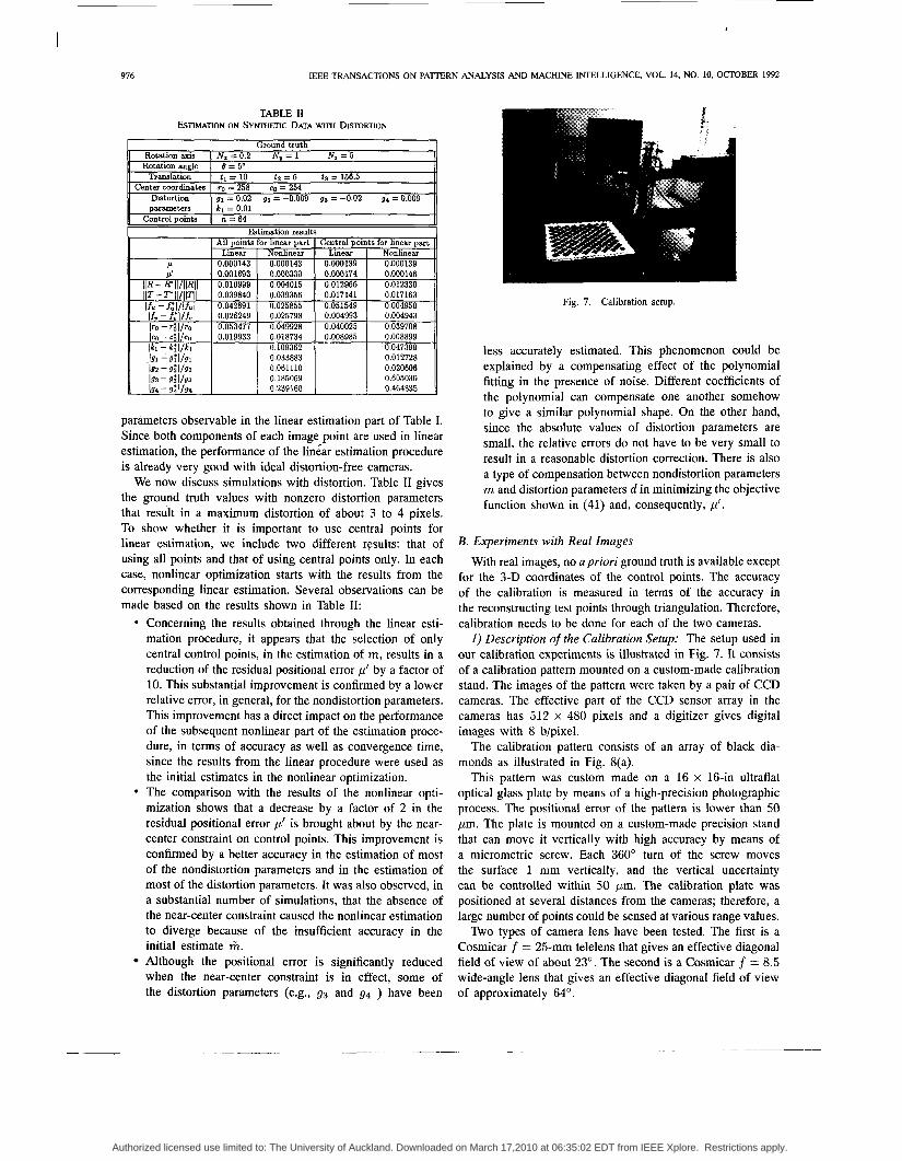
Fig. 7. Calibration setup.

less accurately estimated. This phenomenon could be explained by a compensating effect of the polynomial fitting in the presence of noise. Different coefficients of the polynomial can compensate one another somehow to give a similar polynomial shape. On the other hand, since the absolute values of distortion parameters are small, the relative errors do not have to be very small to result in a reasonable distortion correction. There is also a type of compensation between nondistortion parameters m and distortion parameters d in minimizing the objective function shown in (41) and, consequently, p'.

B. Experiments with Real Images With real images, no apriori ground truth is available except

for the 3-D coordinates of the control points. The accuracy of the calibration is measured in terms of the accuracy in the reconstructing test points through triangulation. Therefore, calibration needs to be done for each of the two cameras.

1) Description of the Calibration Setup: The setup used in our calibration experiments is illustrated in Fig. 7. It consists of a calibration pattern mounted on a custom-made calibration stand. The images of the pattern were taken by a pair of CCD cameras. The effective part of the CCD sensor array in the cameras has 512 x 480 pixels and a digitizer gives digital images with 8 b/pixel.

The calibration pattern consists of an array of black diamonds as illustrated in Fig. 8(a).

This pattern was custom made on a 16 x 16-in ultraflat optical glass plate by means of a high-precision photographic process. The positional error of the pattern is lower than 50 pm. The plate is mounted on a custom-made precision stand that can move it vertically with high accuracy by means of a micrometric screw. Each 360' turn of the screw moves the surface 1 mm vertically, and the vertical uncertainty can be controlled within 50 pm. The calibration plate was positioned at several distances from the cameras; therefore, a large number of points could be sensed at various range values.

Two types of camera lens have been tested. The first is a Cosmicar f = 25-mm telelens that gives an effective diagonal field of view of about 23'. The second is a Cosmicar f = 8.5 wide-angle lens that gives an effective diagonal field of view of approximately 64".


I I

WENG et al.: CAMERA CALIBRATION WITH DISTORTION MODELS 9-7-7

Fig. 8. Calibration pattern and the detected control points: (a) Image of the calibration pattern taken by the first camera with an f = 8.5 lens; (b) vertices of complete diamonds are detected with a subpixel accuracy (marked with crosses). Those vertices are used as control points for the calibration.

2) Control and Test Points: The control points are those points used for calibration, and test points are points used for testing the accuracy of calibration. The 3-D control and test points are chosen to be the vertices of completely visible diamonds. Their spatial positions (E , , yz, z,) are reliably established owing to the accuracy of the calibration plate and the precision stand. The corresponding image-point locations are estimated, with a subpixel accuracy, as the intersections of adjacent edge lines, where each is determined by a least- squares fit to edge points along the side of the diamond. The edge-point locations along each side are determined by a third-order polynomial least-squares fit to the intensity profile across the side. Fig. 8(b) displays an example of those detected control points based on the computed data. The correspondence between the 3-D points and their images was established manually.

During the calibration, the external and nondistortion internal parameters are estimated for each of the two stereo cameras. After the calibration is done, the external and internal parameters of each camera are used to determine the back- projection line of each sensed test point in the world coordinate system. The two back-projection lines of the two cameras reconstruct the 3-D position of the test point in the world coordinate system. This is the process of triangulation. Any error in the calibrated parameters will result in error in the reconstructed 3-D position of the test point. Since we know

the positions of the test points in the world coordinate system, we can use the difference between the 3-D positions of the reconstructed test points and their true positions to indicate the accuracy of the calibration.

In addition to the NSCE, we will also consider three other conventional measures:

The first measure M I is the average norm of the 3-D positional difference between the reconstructed test points and the true test points. The second measure MZ is the average norm of the E-

y plane projection (in the world coordinate system) of the positional error of the test points. Since the two cameras aligned along the y axis, this measure indicates the lateral errors. This measure together with M I provide a feeling of the relative distribution of lateral errors and longitudinal (in depth direction) errors. The third measure M3 is the ratio of the average estimated depth ( z value) to the average absolute depth error. It provides an assessment of the relative accuracy in the depth measurement of a stereo system, and it can be referred to as “one in M3 parts.” However, as we discussed before, M3 will be small with both wide-angle lenses and short distances to the test points.

As discussed in Section IV, among the above four types of measures, only the value of the NSCE directly indicates the accuracy of calibration.

Results for the f=25 mm Telelens: Triangulation tests have been performed for the linear estimation step, which corresponds to a distortion-free model, and the nonlinear estimation step, which uses our complete distortion model. In this way, we can see whether the distortion model brings about any improvement for this type of lens. Only central points are used as control points for the linear estimation procedure and its residual measurement. The calibration plate is positioned at four positions: z = 0, z = -50, z = -100, and z = -200. The points at z = -100 are used as test points, and the remaining points are used as control points for calibration. Table I11 lists the results obtained. The results of triangulation are measured in the coordinate system centered at the first camera.

On the basis of the M I , Mz, and M3 measurements, it can be observed from Table I11 that the triangulation accuracy has been significantly improved by the estimation of the distortion parameters. In particular, M3 gives an indication of the increased accuracy in depth estimation. Comparison between the values of the image positional error parameter p’ confirms the improvement of the nonlinear optimization over the linear estimation procedure even though the later is measured only over central points.

The performance of calibration is directly indicated by the NSCE values. As presented in Table 111, the measured NSCE value of the linear estimation is equal to 1.7478, which is about 75% larger than 1, which means that the accuracy of this calibration has not reached the potential accuracy allowed by the image resolution. The NSCE value of the nonlinear estimation is, however, just about 6% larger than 1, which indicates a good calibration.


I I

978

Residual p' Control points n Rotation axis N.

N,

IEEE TRANSACTIONS ON PATTERN ANALYSIS AND MACHINE INTELLIGENCE, VOL. 14, NO. 10, OCTOBER 1992

camera camera camera camera 0.000287 0.000234 0.000253 0.000207

73 77 264 284 0.6202 -0.0171 0.6194 -0.0173 -0.7801 -0.9834 -0.7807 -0.9831

TABLE 111 CALIBRATION RESULTS FOR THE f = 25 mm LENS AND TESTING

N; Rotation angle (") 0 7hmlation (mm) tl

12

h Results of Calibration Linear I Nonlinear

First I Second 1 First I Second

-0.0825 -0.1806 -0.0829 -0.1822 11.5572 8.8356 11.5618 8.8382 -162.74 -158.43 -162.76 -158.46 '

-190.99 -189.21 -190.98 -189.18 1s

Focal length f, f.

Center ro coordinates CO

Distortion 11

parameters 91

gz g3

866.03 901.59 864.89 901.07 -1923.20 -1914.07 -1921.81 -1913.68 1587.44 1580.53 1587.21 1580.38 257.28 273.15 257.33 273.22 275.13 270.59 275.14 270.63

0.0 0.0 0.2632 0.2325 0.0 0.0 -0.000110 -0.002818 0.0 0.0 0.003521 0.008344 0.0 0.0 0.004880 0.007216

I -" g4 I 0.0 I 0.0 I 0.0 I 0.0 I

Results of Triangulation Test

z 317.67mm Nonlinear 317.53mm Average depth

Test points n 188 188 Test Mi 3.7574" 2.19lOmm

Linear

The absolute values of the radial and tangential parameters do not directly give the relative amount of distortion in the cameras. As can be seen in (20), k1 is the coefficient of the third power of image coordinates, and the si's are the coefficients of the second power. From (4), the maximum absolute value of C is around 240/fu N 0.125, and that of 6 is 256/fv N 0.162. According to the measured distortion parameters, the maximum (symmetrical) radial distortion discussed in Section 11-B-1 is about five to seven times larger than that of the combination of decentering and thin prism distortions. The coefficient of radial distortion also indicates that the maximum radial distortion is about 3 to 4 pixels, which occurs at the border of the images.

We have also modified this experiment so that all the control points, and not just central points, are used for the linear estimation. This modification caused the linear estimation to give a slightly worse result compared with that listed in Table 111. From this worse result, the following nonlinear estimation procedure reached a triangulation accuracy similar to the corresponding one shown in Table 111, but it took 130% more CPU time to converge.

In the above experiments, the plane of test points is located between the planes of control points. To investigate the ability of the calibrated cameras to measure points beyond the range of control points, we let the points at z = -50 and z = -200 be control points and the points at z = 0 be test points. The measured test parameters from the nonlinear estimation are MI = 0.6476, M2 = 0.2335, M3 = 1615.7 mm, and NSCE = 1.0735, which are nearly as good as those listed in Table 111. For example, the NSCE value increased by about 1.3%.

4) Results for the f=S mm Wide-Angle Lens: With a wide- angle lens, the distortion is expected to be more significant than with a telelens. First, we present in Table IV the results

Mz M3

NSCE

parameters

TABLE IV CALIBRATION RESULTS AND TESTING FOR THE f = 8 mm LENS WITH A DISTORTION-FREE CAMERA MODEL

I Results of Calibration I

0.9098mm 0.6773mm 87.340 170.30 2.9952 3.9793

n __.._~ ~

I Nonlinear Linear First I Second I First I Second

with a distortion-free camera model. Two sets of results are presented. The first set comes from

the linear estimation procedure using central control points. The second set comes from the nonlinear estimation procedure assuming d = 0 and using the results from linear estimation as initial estimates. The motivation of this arrangement is to show what will happen if a distortion-free camera model is applied to cameras with considerable distortion.

As can be seen from Table IV, the accuracy is very poor for both linear and nonlinear estimation procedures. Since the result from the linear estimation is poor, the nonlinear estimation procedure with d = 0 fails to find good estimates and leads to an even worse NSCE value. The residual parameter p' of the nonlinear estimation is much larger than that of the linear estimation because the former was measured in the entire image plane where boundary regions sustain significant distortion. The poor performance of the nonlinear estimation can be explained as follows. The procedure tries to fit a distortion-free model to the images with significant distortion, but it cannot fit well. To further minimize the objective function in (41), the nondistortion parameter m has to be changed, which results in a worse m. Such a worse m directly leads to a bad NSCE. This is the consequence of neglecting all kinds of distortions.

Table V shows the results from the nonlinear optimization procedure with different completeness of distortion parameters: a) radial distortion only and b) our complete distortion model. The results from the linear estimation procedure shown in Table IV were used as the initial estimates.

Compared with the case of f = 25 mm in Table 111, the residual values of p' in Table V are larger mainly because the focal length of the cameras here is much shorter, and consequently, the size of the normalized image plane in the


WENG et al.: CAMERA CALIBRATION WITH DISTORTION MODELS

Radial only . First Second

camera camera Residual p' 0.001245 0.001573 Control points n 428 424 Rotation axis N. 0.9884 -0.9524

979

Radial & tangential First Second

camera camera 0.000992 0.001064

428 424 0.9851 -0.9482

TABLE V CALIBRATION RESULTS AND TESTING FOR THE f = 8

mm LENS WITH DISTORTION CAMERA MODELS

- - Test points n Test Mi parameters Mz

MS NSCE

188 188 0.5811" 0.4653mm 0.3149mm 0.2599mm

722.86 897.46 1.4081 1.1627

i

Focal length fv I 525.58 I 526.48 1 525.62 1 525.77

Center m I 240.90 I 244.47 I 241.15 I 244.70 coordinates

parameters

Results of Triangulation Test 1 Radial only 1 Radial & tangential

Average deuth z I 314.03" I 313.84"

space (G, ~) defined in (4) is much larger. In addition, because of the shorter focal length, the value of is smaller as has been discussed. Again, the parameter value that directly indicates the accuracy of the calibration is the NSCE. From Table V, we can see that with only radial distortion under consideration, the NSCE value is 41% larger than 1, whereas with our complete distortion model, the NSCE value reduces to 1.1627. With this value of NSCE, we know that most of the distortion has been corrected, compared with the effect of digitization noise.

These results show the importance of accommodating distortion and, in particular, the tangential distortion. Although correcting symmetrical radial distortion leads to significant improvement from the distortion-free model, further correcting remaining distortion makes the NSCE decrease from 1.41 to 1.16. The estimated distortion parameters indicate that the maximum symmetrical radial distortion is about 23 pixels, whereas the maximum of the combination of decentering and thin prism distortions is around 3 pixels. Notice that the estimated value of the radial distortion parameter k l is virtually the same from a radial distortion-only model to the complete model, which appears to indicate that the parameters of the decentering and thin prism distortions do little to compensate the radial distortion or vice versa. It is also interesting to note from Table V that for both cameras, the estimated distortion parameter g 3 is significantly larger than other distortion parameters gis , which implies that the axis of maximum tangential distortion is roughly aligned with the v axis. According to our derivation of the distortion parameters, the parameters j 1 , c p o in (9) and i l , cp1 in (12) can be computed from 9 1 , g 2 , 93, and 9 4 . For example, for the first camera, the axis of maximum tangential decentering distortion is computed as cpo = -74.20' from the U direction.

VI. SUMMARY AND CONCLUSIONS

With a goal of investigating the effects of radial and tangential distortion, the distortion of a camera is modeled by a combination of three typical effects: radial, decentering, and thin prism distortions. These three effects result in five distortion parameters that accommodate up to third-order terms.

In the calibration procedure, nondistortion parameters are first computed using a closed-form solution, and they are then used as initial estimates for further nonlinear optimization. The nondistortion and distortion parameters are decoupled in our procedure so that their harmful interactions are suppressed, which makes the nonlinear optimization more stable.

We have introduced a type of normalized accuracy measure for stereo or single camera calibration, which can be used to evaluate the accuracy of calibration and compare different calibrations without being significantly affected by the differences among systems.

Our experimental results have demonstrated the performance of our approach with both synthetic and real data. Generally, a wide-angle lens causes more distortion than a telelens. Therefore, distortion correction is more important for wide-angle lenses. Symmetrical radial distortion correction results in significant improvement. Correcting tangential distortion also leads to a considerable improvement over just correcting radial distortion.

APPENDIX

The solution of R that satisfies

where C = [ C I C ~ . . . Cn] and D = [ D l D z . . . D,], subject to R (which is a rotation matrix), is as follows.

Define a 4 by 4 matrix B by

n B=CBTB~ i=l

where

(53)

where [a] is a mapping from a 3-D vector to a 3 by 3 matrix:

Let q = (no, 4 1 , q2 , q3)T be a unit eigenvector of B associated with the smallest eigenvalue. The solution of rotation matrix R in (51) is shown at the top of the next page. For proofs, see [12], [5], and [14].


980 IEEE TRANSACTIONS ON PAlTERN ANALYSIS AND MACHINE INTELLIGENCE, VOL. 14, NO. 10, O(JT0BER 1992

ACKNOWLEDGMENT

The instrumentation support from H. Nguyen is gratefully acknowledged.

REFERENCES

Y. I. Abdel-Aziz and M. M. Karara, “Direct linear transformation into object space coordinates in close-range photogrammetry,” in Proc. Symp. Close-Range Photogrammetry (Urbana, IL), Jan. 1971, pp. 1-18. 0. Bottema and B. Roth, Theoretical Kinematics. Amsterdam: North- Holland, 1979. D. C. Brown, “Decentering distortion of lenses,” Photogrammetric Eng. Remote Sensing, May 1966, pp. 444462. W. Faig, “Calibration of close-range photogrammetric systems: Math- ematical formulation,” Photogrammetric Eng. Remote Sensing, vol. 41, no. 12, pp. 1479-1486, Dec. 1975. 0. D. Faugeras and M. Hebert, “A 3-D recognition and positioning algorithm using geometrical matching between primitive surfaces,” in Proc. 8th Int. Joint Conf Artificial Intell. (Karlsruhe, W. Germany), Aug. 1983, pp. 996-1002. 0. D. Faugeras and G. Toscani, “Calibration problem for stereo,” in Proc. Int. Conf Comput. Vision Putt. Recogn. (Miami Beach, FL), June

D. B. Gennery, “Stereo-camera calibration,” in Proc. loth Image Un- derstanding Workshop, 1979, pp. 101-108. S. Ganapathy, “Decomposition of transformation matrices for robot vision,” in Proc. IEEE Int. Conf Robotics Auromut. (Atlanta), Mar. 1984, pp. 130-139. A. Isaguirre, P. Pu, and J. Summers, “A new development in camera calibration calibrating a pair of mobile cameras,” in Proc. IEEE Int. Conf Robotics Automat. (St. Louis), Mar. 1985, pp. 74-79. R. K. Lenz and R. Y. Tsai, “Techniques for calibration of the scale factor and image center for high accuracy 3D machine vision metrology,” in Proc. IEEE Int. Con$ Robotics Automat. (Raleigh, NC), Mar. 1987, pp. 68-75. Manual of Photogrammetry. Amer. Soc. Photogrammetry, 1980, 4th ed. M. D. Shuster, “Approximate algorithms for fast optimal attitude com- putation,’’ in Proc. A M Guidance Contr. Spec. Con$ (Palo Alto, CA), Aug. 1978, pp. 88-95. R. Y. Tsai, “A versatile camera calibration technique for high-accuracy 3D machine vision metrology using off-the-shelf TV cameras and lenses,” IEEE .I. Robotics Automat., vol. RA-3, no. 4, pp. 323-344, Aug. 1987. J. Weng, T. S. Huang, and N. Ahuja, “Motion and structure from two perspective views: Algorithm, error analysis and error estimation,” IEEE Trans. Putt. Anal. Machine Intell., vol. 11, no. 5, pp. 451476, May. 1989. K. W. Wong, “Mathematical formulation and digital analysis in close- range photogrammetry,” Photogrammetric Eng. Remote Sensing, vol. 41, no. 11, pp. 1355-1373, Nov. 1975.

1986, pp. 15-20.

Recherche Informatique been associated with Eci

Juyang Weng (S’S-M’88) received the B.S. degree from Fudan University, Shanhai, China, in 1982 and the M.S. and Ph.D. degrees from the University of Illinois, Urbana-Champaign, in 1985 and 1988, respectively, all in computer science.

From September 1984 to December 1988, he was a research assistant at the Coordinated Science Laboratory, University of Illinois. In the summer of 1987, he was employed at IBM Los Angeles Scienfific Center, Los Angeles, CA. Since January 1989, he has been a researcher at the Centre de de MontrCal, MontrCal, Canada, while he has also

,le Polytechnique de Montreal. Since October 1990, he has held a visiting assistant professor-position at the University of Illinois at Urbana-Champaign. He is now an assistant professor with the Department of Computer Science, Michigan State University. His current research interests include computer vision, image processing, neural networks, object modeling and representation, parallel architecture for image processing, autonomous navigation, and artificial intelligence.

Paul Cohen received the B.S. degree in electronics from the lnsitut National Polytechnique de Toulouse, France, in 1970 and the MSc. and Ph.D. degrees in electrical engineering from the UniversitC de Sherbrooke in Quebec in 1972 and 1976, respectively.

Since 1978, he has been with the Department of Electrical and Computer Engineering, Ecole Polytechnique de MontrCal, MontrCal, Canada, where he is presently a full professor in charge of the Perception and Robotics Laboratory. His research

interests are in image processing, computer vision, and pattern recognition.

Marc Herniou received the engineering degree in electronics and computer science from the Univer- sit6 de Paris-Sud-Orsay in 1989.

In 1989, he was at the Ecole Polytechnique de Montrtal, MontrCal, Canada, where he worked on computer vision. He is currently a Research and Development engineer in Schlumberger, France.


camera calibration with distortion models and accuracy ... · model. in the second step, the...

Documents