calibration risk for exotic options - econstor

SFB 649 Discussion Paper 2006-001

Calibration Risk for Exotic Options

Kai Detlefsen*

Wolfgang K. Härdle**

* CASE - Center for Applied Statistics and Economics, Humboldt-Universität zu Berlin, Germany

This research was supported by the Deutsche Forschungsgemeinschaft through the SFB 649 "Economic Risk".

http://sfb649.wiwi.hu-berlin.de

ISSN 1860-5664

SFB 649, Humboldt-Universität zu Berlin Spandauer Straße 1, D-10178 Berlin

SFB

6

4 9

E

C O

N O

M I

C

R

I S

K

B

E R

L I

N

Calibration Risk for Exotic Options

K. Detlefsen and W. K. Hardle

CASE - Center for Applied Statistics and EconomicsHumboldt-Universitat zu Berlin

Wirtschaftswissenschaftliche FakultatSpandauer Strasse 1, 10178 Berlin, Germany

AbstractOption pricing models are calibrated to market data of plain vanil-

las by minimization of an error functional. From the economic view-point, there are several possibilities to measure the error between themarket and the model. These different specifications of the error giverise to different sets of calibrated model parameters and the resultingprices of exotic options vary significantly. These price differences oftenexceed the usual profit margin of exotic options.

We provide evidence for this calibration risk in a time series ofDAX implied volatility surfaces from April 2003 to March 2004. Weanalyze in the Heston and in the Bates model factors influencing theseprice differences of exotic options and finally recommend an error func-tional. Moreover, we determine the model risk of these two stochasticvolatility models for the time series and consider its relation to cali-bration risk.

Key Words: calibration risk, calibration, model risk, Hestonmodel, Bates model, barrier option, cliquet option

JEL Classification: C13, G12

Acknowledgement: This research was supported by DeutscheForschungsgemeinschaft through the SFB 649 ”Economic Risk” andby Bankhaus Sal. Oppenheim. The authors would like to thank BerndEngelmann and Peter Schwendner for helpful discussions.

1 Introduction

Recently, there has been a considerable interest, both from a practicaland a theoretical point of view, in the risks involved in option pric-ing. Schoutens et al. (2004) have analyzed model risk in an empiricalstudy and Cont (2004) has put this risk into a theoretical framework.Another source of risk is hidden in the calibration of models to marketdata. This calibration risk exceeds often the profit margin for exoticoptions and hence is also of fundamental interest for the banking in-dustry. Moreover, calibration risk exists even if an appropriate modelhas been chosen and model risk does not exist anymore.

Calibration risk arises from the different possibilities to measurethe error between the observations on the market and the correspond-ing quantities in the model world. A natural approach to specifythis error is to consider the absolute price (AP) differences, see e.g.Schoutens et al. (2004). But the importance of absolute price differ-ences depends on the magnitude of these price. Hence, another usefulway for measuring the error are relative price (RP) differences, see e.g.Mikhailov et al. (2003). As models are often judged by their capabilityto reproduce implied volatility surfaces other measures can be definedin terms of implied volatilities. There are again the two possibilities ofabsolute implied volatilities (AI) and relative implied volatilities (RI).We consider these four ways to measure the difference between modeland market data and explore the implications for the pricing of exoticoptions.

To this end, we focus on the popular stochastic volatility modelof Heston. In order to analyze the influence of the goodness of fit oncalibration risk we consider in addition the Bates model which is anextension of the Heston model with similar qualitative features. Thesetwo models are calibrated to plain vanillas on the DAX. In order toget reliable results we use a time series of implied volatility surfacesfrom April 2003 to March 2004. Because of the computationally in-tense Monte Carlo simulations for the pricing of the exotic options weconsider only one trading day in each week of this period. As exoticoptions we consider down and out puts, up and out calls and cliquetoptions for 1, 2 or 3 years to maturity. In this framework we determinethe size of calibration risk and analyze factors influencing it.

Besides calibration risk there is also model risk which representswrong prices because a wrong parametric model has been chosen. Weconsider also model risk between the Heston and the Bates model and

1

analyze the relation between the two forms of risk in pricing exoticoptions.

Section 2 introduces the models and describes their risk neutraldynamics that we use for option pricing. Moreover, this section con-tains information about the data used for the calibration. Section 3describes the calibration method and defines the error functionals an-alyzed in this work. The goodness of fit is shown by representativesurfaces and statistics on the errors. In Section 4, we present the exoticoptions that we consider for calibration risk and price these productsby simulation. In Section 5, we analyze the model risk for the twostochastic volatility models under the four error functionals. In thelast Section 6, we summarize the results and draw our conclusions.

2 Models and Data

In this section, we describe briefly the Heston model and the Batesmodel for which we are going to analyze calibration risk. Moreover,we provide some descriptive statistics of the implied volatility surfacesthat we use as input data for the calibration.

2.1 Heston model

We consider the popular stochastic volatility model of Heston (1993):

dSt

St= µdt+

√VtdW

1t

where the volatility process is modelled by a square-root process:

dVt = ξ(η − Vt)dt+ θ√VtdW

2t

and W 1 and W 2 are Wiener processes with correlation ρ.

The volatility process remains positive if its volatility θ is smallenough with respect to the product of the mean reversion speed ξ andthe average volatility level η:

ξη >θ2

2. (1)

2

The dynamics of the price process are analyzed under a martingalemeasure under which the characteristic function of log(St) is given by:

φHt (z) = exp{ −(z2 + iz)V0

γ(z) coth γ(z)t2 + ξ − iρθz

}

×exp{ ξηt(ξ−iρθz)

θ2 + iztr + iz log(S0)}

(cosh γ(z)t2 + ξ−iρθz

γ(z) sinh γ(z)t2 )

2ξη

θ2

where γ(z) def=√θ2(z2 + iz) + (ξ − iρθz)2, see e.g. Cont et al. (2004).

2.2 Bates model

Bates (1996) extended the Heston model by considering jumps in thestock price process:

dSt

St= µdt+

√VtdW

1t + dZt

dVt = ξ(η − Vt)dt+ θ√VtdW

2t

where Z is a compound Poisson process with intensity λ and jumps kthat have a lognormal distribution:

log(1 + k) ∼ N(log(1 + k)− δ2

2, δ2).

We analyze the dynamics of this model under a martingale measureunder which the characteristic function of log(St) is given by:

φBt (z) = exp{tλ(e−δ2z2/2+i{log(1+k)− 1

2δ2}z − 1)}

× exp{ −(z2 + iz)V0

γ(z) coth γ(z)t2 + ξ − iρθz

}

×exp{ ξηt(ξ−iρθz)

θ2 + izt(r − k) + iz log(S0)}

(cosh γ(z)t2 + ξ−iρθz

γ(z) sinh γ(z)t2 )

2ξη

θ2

where γ(z) def=√θ2(z2 + iz) + (ξ − iρθz)2, see e.g. Cont et al. (2004).

The Bates model has eight parameters while the Heston model hasonly five parameters. Because of these three additional parameters theBates model can better fit observed surface but parameter stability ismore difficult to achieve.

3

mean number mean number mean money-of maturities of obervations ness range

short maturities 3.06 64 0.553(0.25 ≤ T < 1.0)long maturities 5.98 76 0.699

(1.0 ≤ T )total 9.04 140 0.649

Table 1: Description of the implied volatility surfaces.

2.3 Data

Our data consists of EUREX-settlement volatilities of European op-tions on the DAX. We consider the time period from April 2003 toMarch 2004. Since March 2003 the EUREX trades plain vanillas withmaturities up to 5 years. Until March 2004 it has not changed itsrange of products. Hence, the data is homogeneous in sense that theimplied volatility surfaces are derived from similar products.

From this time period we analyze the surfaces from all the Wednes-days when trading has taken place. Thus, we consider 51 impliedvolatility surfaces. We exclude observations that are deep out of themoney because of illiquidity of these products. More precisely, we con-sider only options with moneyness m = K/S0 ∈ [0.75, 1.35] for smalltimes to maturity T ≤ 1. As we analyze exotic options with maturityin 1, 2 or 3 years we exclude also plain vanillas with time to maturityless than 3 months.

Some information about the resulting implied volatility surfacesare summarized in table 1. The surfaces contain in the mean 140transformed prices and nine maturities with a mean moneyness rangeof 65%.

The values of the underlying in the considered period are shown infigure 1. This figure contains also the (interpolated) implied volatilitiesfor 1 year to maturity with strike at spot level. Hence, the market ofthe DAX went up in this period while the implied volatilities wentdown as figure 1 shows.

We approximate the risk free interest rates by the EURIBOR. Oneach trading day we use the yields corresponding to the maturities ofthe implied volatility surface. As the DAX is a performance index it

4

01-Apr-03 01-Oct-03 31-Mar-042400

2600

2800

3000

3200

3400

3600

3800

4000

4200D

AX

01-Apr-03 01-Oct-03 31-Mar-040.18

0.2

0.22

0.24

0.26

0.28

0.3

0.32

0.34

0.36

0.38

impl

ied

vola

tiliti

es

Figure 1: DAX and ATM implied volatility with 1 year to maturity on thetrading days from 01 April 2003 to 31 March 2004.

is adjusted to dividend payments. Thus, we do not consider dividendpayments explicitly.

3 Calibration

In this section, we specify the calibration routine and describe thefour error functionals. The calibration results illustrate that the plainvanilla prices can be well replicated by the Heston and the Batesmodel.

3.1 Calibration method

Carr & Madan (1999) found a representation of the price of a Euro-pean call option by one integral for a whole class of option pricingmodels. Their method that is applicable to the Heston (1993) modelis based on the characteristic function of the log stock price under therisk neutral measure.

Carr and Madan showed that the price C(K,T ) of a European calloption with strike K and maturity T is given by

C(K,T ) =exp{−α ln(K)}

π

∫ +∞

0exp{−iv ln(K)}ψT (v)dv

for a (suitable) damping factor α > 0. The function ψT is given by

ψT (v) =exp(−rT )φT {v − (α+ 1)i}α2 + α− v2 + i(2α+ 1)v

5

where φT is the characteristic function of log(ST ), see Section 2.For the minimization we consider the following four objective func-

tions based on the root weighted square error:

AP def=

√√√√ n∑i=1

wi(Pmodi − Pmar

i )2

RP def=

√√√√ n∑i=1

wi(Pmod

i − Pmari

Pmari

)2

AI def=

√√√√ n∑i=1

wi(IV modi − IV mar

i )2

RI def=

√√√√ n∑i=1

wi(IV mod

i − IV mari

IV mari

)2

where mod refers to a model quantity and mar to a quantity observedon the market, P to a price and IV to an implied volatility. The indexi runs over all nt observations of the surface on day t. The weights wi

are non negative with∑

iwi = 1. Hence, the objective functions canbe interpreted as mean average errors.

We choose the weights in such a way that on each day all maturitieshave the same influence on the objective function. In order to makedifferent surfaces comparable each maturity gets the weight 1/nmat

where nmat denotes the number of maturities in this surface. More-over, we assign the same weight to all points of the same maturity.This leads to the weights

widef=

1nmatni

str

where nistr denotes the number of strikes with the same maturity as

observation i. This weighting leads asymptotically to a uniform den-sity on each maturity.

Given these weights we measure the average time to maturity ofan implied volatility surface by a modified duration:

n∑i=1

τiwi∑ni=1wi

6

where τi is the time to maturity of the option i. The mean durationof the 51 surfaces is 2.02 and the minimal (maximal) is 1.70 (2.30).Thus, the point of balance for the maturities lies around 2 for our timeseries of surfaces. As we analyze exotic options with 1, 2 or 3 yearstime to maturity this point of balance confirms a correct weighting forour purposes.

As prices we consider only out of the money prices. Thus, we usecall prices for strikes higher (or equal) than the spot and put prices forstrikes below the spot. This approach ensures to compare only pricesof similar magnitude. It has no impact on the errors based on impliedvolatilities. Because of the put call parity the use of OTM optionshas nor an impact on the absolute price error (AP). But the relativeprices are weighted in such a way that the observations around thespot receive less weight. Hence, only the relative price error (RP) isinfluenced by this choice of prices.

In order to estimate the model parameters we apply a stochasticglobal optimization routine and minimize the objective functions withrespect to the model parameters. In addition to some natural con-straints on the range of the parameters we have taken into accountinequality 1 that ensures the positivity of the volatility process.

Sometimes the objective function that is minimized contains inaddition to the error measure a regularization term. Regularizationcan be necessary for two reasons: The error function may have severalglobal minima and thus the regularization is necessary in order to geta unique minimum. Besides this static problem it is also important tofind parameters on subsequent days that lead to similar prices (andgreeks) of exotic options. This time stability is essential for the prac-tical applicability of the calibration. We have discovered in tests onsimulated and real data that our algorithm finds a unique solutionwhatever the starting conditions are. As we do not consider subse-quent trading days in our analysis the time stability is not essentialin our case. Hence we omit a regularization term.

3.2 Calibration results

We have considered the implied volatility surfaces of each Wednesdayin the period from April 2003 to March 2004 on which trading hastaken place. Thus, we have analyzed 51 surfaces. Each of these hasbeen calibrated with respect to the four error functions described inSection 3.1. These calibrations have been done for the Heston and the

7

mean AP RP AI RIobjective fct. [E−2] [E−2] [E−2]

AP 7.3 9.7 0.81 3.1RP 11. 6.1 0.74 2.9AI 9.4 7.3 0.68 2.6RI 8.8 7.0 0.70 2.5

Table 2: Calibration errors in the Heston model for 51 days.

Bates model.The resulting errors of these 408 calibrations have been summa-

rized in table 2 for the Heston model and in table 3 for the Batesmodel. Descriptive statistics on the calibrated parameters are givenin the appendix in table 9 for the Heston model and in table 10 for theBates model. Figure 2 shows the fit of the implied volatility surfacein the Heston model on a day that is representative for the AI error.

Table 2 reports in each line the means of the four errors when theobjective function given in the left column is minimized. In the Hestonmodel, we get a mean absolute price error of 7.3 and a mean relativeprice error of 9.7% when we calibrate with respect to AP. Using theRP error functional we get the opposite result with a mean absoluteprice error of 11 and a mean relative price error of 6.1%. The errorsbased on implied volatilities are smaller for the RP objective functionthan for the AP objective function. The results for the AI and RIobjective functionals differ only slightly: the mean absolute impliedvolatility error is about 0.68% and the mean relative implied volatil-ity error is about 2.5%. Moreover, the price errors for these objectivefunctions lie between the price errors of the other two objective func-tions. The calibration w.r.t. RI gives the best overall fit because ithas the smallest RI error and the second best errors for the rest. Themeaning of these error measures is illustrated by figure 2 which showsan implied volatility fit that is representative for an AI error of 0.68%.In order to make the AP errors comparable for different days (withdifferent values of the spot) we have computed the mean of AP/DAXas 0.21, 0.34, 0.27, 0.25 for the four error functionals.

The calibrated parameters which are described in the appendix bytable 9 form two groups because the parameters for the RP, AI and RIcalibration are quite similar. The start volatility V0 and the averagevolatility level η are both about 7% for all objective functionals. For

8

mean AP RP AI RIobjective fct. [E−2] [E−2] [E−2]

AP 7.0 13. 0.76 2.8RP 12. 5.1 0.67 2.6AI 8.9 6.4 0.60 2.3RI 8.7 6.2 0.62 2.2

Table 3: Calibration errors in the Bates model for 51 days.

the AP calibration we get a reversion speed ξ = 0.9, a volatility ofvolatility of θ = 0.34 and a correlation ρ = −0.82. The other cali-brations lead to similar parameters with a reversion speed ξ = 1.3, avolatility of volatility of θ = 0.44 and a correlation ρ = −0.75. As thecorrelations are significantly below −1 the calibrated Heston modelshave really two stochastic factors.

The Bates model exhibits similar qualitative results as the Hestonmodel: The AP and the RP calibrations differ widely while the AIand the RI calibrations lead to similar results. The Bates model canregarded as an extension of the Heston model. The additional threeparameters for the jumps in the spot process lead for all errors func-tionals to better calibration results: The AP error is reduced (in themean) by 4%, RP error by 16%, the AI and the RI error both by 12%.

The calibrated parameters of the Bates model are given in table 10.As in the Heston model they form two groups with the AP calibrationon the one hand and the RP, AI and RI calibrations on the other hand.The parameters ξ, η, θ and V0 are similar to the calibrations for theHeston model. Only the correlation ρ rises to a level of −0.93 for allobjective functions. Hence, this criterion for distinguishing betweenthe two groups disappears. It is replaced by the expected number ofjumps per year: For the AP calibration we expect (in the mean) ajump every three years while we expect every two years a jump forthe other calibrations. It is interesting that all calibrations lead to amean jump up of about +8% for the returns. The expected jumpsupwards correspond to the market going up as shown in figure 1.

Schoutens et al. (2004) found that the Heston and the Bates op-tion model can both be calibrated well to the EuroStoxx50. In sum-marizing the results of this section we can say that also DAX impliedvolatility surfaces can be replicated well by these models for differenterror functionals. As Schoutens et al. (2004), we find that the Bates

9

0.6 0.8 1 1.2 1.4 1.60.2

0.3

0.4

0.5

0.6 0.8 1 1.2 1.4 1.60.2

0.25

0.3

0.35

0.4

0.6 0.8 1 1.2 1.4 1.60.2

0.25

0.3

0.35

0.4

0.6 0.8 1 1.2 1.4 1.60.2

0.25

0.3

0.35

0.4

0.6 0.8 1 1.2 1.4 1.60.2

0.25

0.3

0.35

0.4

0.6 0.8 1 1.2 1.4 1.60.2

0.25

0.3

0.35

0.4

0.6 0.8 1 1.2 1.4 1.60.2

0.25

0.3

0.35

0.4

0.6 0.8 1 1.2 1.4 1.60.2

0.25

0.3

0.35

0.4

0.6 0.8 1 1.2 1.4 1.60.2

0.25

0.3

0.35

0.4

0.6 0.8 1 1.2 1.4 1.60.2

0.25

0.3

0.35

0.4

Figure 2: Implied volatilities in the Heston model for the maturities 0.26,0.52, 0.78, 1.04, 1.56, 2.08, 2.60, 3.12, 3.64, 4.70 (left to right, top to bottom)for AI parameters on 25/6/2003. Red solid: model, blue dotted: market.X-axis: moneyness.

10

model gives only slightly better fits for the AP calibration. In additionwe have shown that it leads to a considerable improvement in the fitfor the other objective functions.

4 Exotic Options

We come now to the analysis of the price differences of exotic optionsfor calibrations w.r.t. different error measures. We consider barrierand cliquet options. The prices of these products are calculated byMonte Carlo simulations using Euler discretizations.

4.1 Simulation

We price all exotic options by Monte Carlo simulations. To this end,we use for each derivate product 1000000 paths generated by Eulerdiscretization, see e.g. Glasserman (2004). For each exotic option weconsider three maturities: 1 year, 2 years and 3 years. We analyzethree exotic options: up & out calls, down & out puts and cliquetoptions. These products are described in the following sections whereremaining parameters are also specified.

The payoffs of barrier options depend on the minimum or maxi-mum of the underlying price process in some time interval. We ap-proximate this quantity by a discrete minimum with one observationfor each trading day. Thus, we use 250 time steps to simulate a processfor a year.

The calibration results are presented in following sections togetherwith a discussion of the options. The accuracy of the Monte Carloresults is given by the relative standard error in table 4. Thus, thistable confirms that the estimators have sufficiently small variance after1000000 paths compared to the price differences we observe in tables5 to 7.

4.2 Barrier Options

For the barrier options that are very popular on the market we con-sider two types: up & out calls and down & out puts.

11

Heston BatesT = 1 T = 2 T = 3 T = 1 T = 2 T = 3

up and out calls 0.17 0.10 0.08 0.17 0.11 0.09down and out puts 0.18 0.11 0.08 0.19 0.12 0.10

cliquet options 0.06 0.05 0.05 0.07 0.06 0.05

Table 4: Maximal relative standard error in percent of Monte Carlo simula-tions. (Maximum over all time points and all objective functions)

4.2.1 Up and out call options

The prices of up and out calls with strike K, barrier B and maturityT on an underlying (St) are given by

exp(−rT ) E[(ST −K)+1{MT <B}]

where

MTdef= max

0≤t≤TSt.

We choose as strike K and barrier B

K = 1− 0.1TB = 1 + 0.2T

where T denotes time to maturity. Up and out calls with such strikesand barriers are widely traded on the market.

Up and out call options have the payoff profile of European calloptions if the underlying has not fallen below the barrier. Otherwisetheir payoff is zero. Thus, up and out calls are path dependent exoticoptions.

We want to analyze the difference between the prices of the exoticoptions when the underlying model has been calibrated w.r.t. differenterrors. To this end, we have calibrated the Heston and the Bates modelto implied volatility or price data on each day w.r.t. the four errorfunctionals introduced in Section 3.1. Hence we have four time seriesof calibrated model parameters that are described in Section 3.2. ByMonte Carlo simulations we calculate on each day the prices of up andout calls for the four sets of model parameters. In this way we get four

12

AP/RP AP/AI AP/RI RP/AI RP/RI AI/RI

0.9

0.95

1

1.05

1.1

1.15

1.2

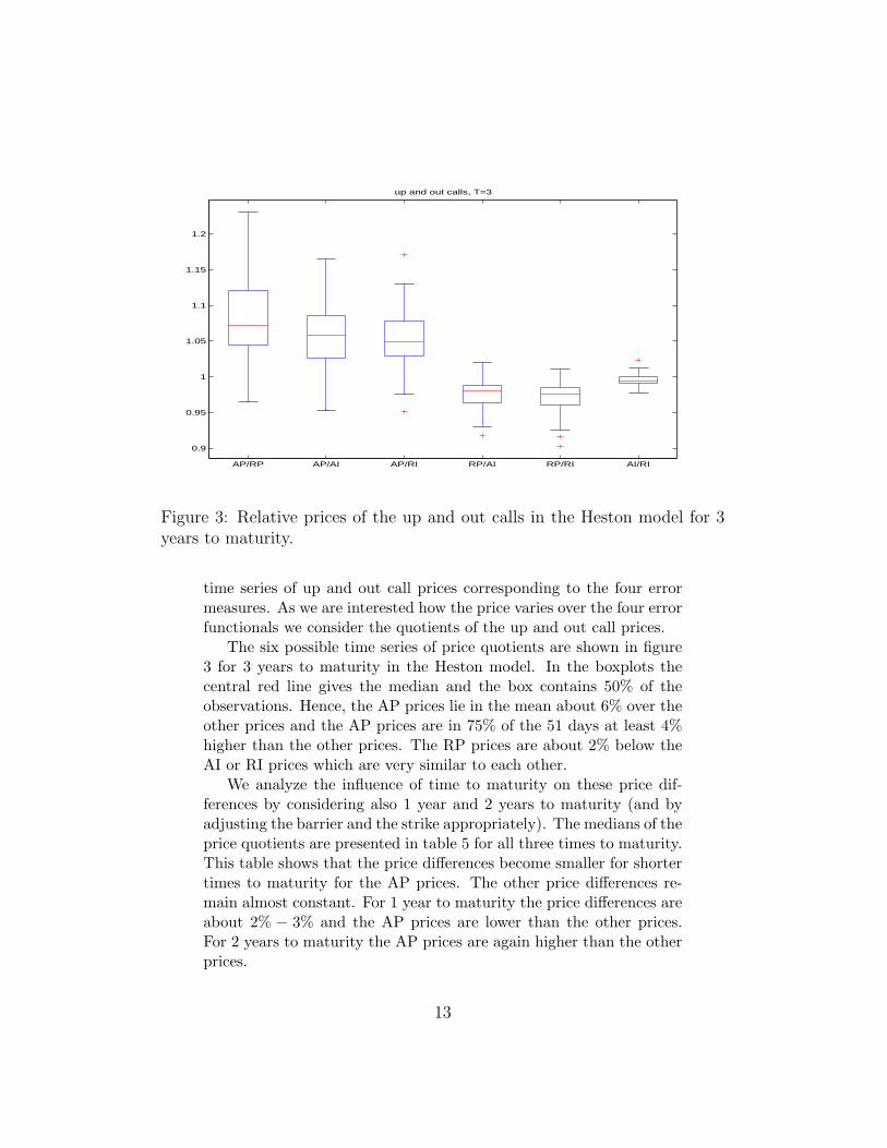
up and out calls, T=3

Figure 3: Relative prices of the up and out calls in the Heston model for 3years to maturity.

time series of up and out call prices corresponding to the four errormeasures. As we are interested how the price varies over the four errorfunctionals we consider the quotients of the up and out call prices.

The six possible time series of price quotients are shown in figure3 for 3 years to maturity in the Heston model. In the boxplots thecentral red line gives the median and the box contains 50% of theobservations. Hence, the AP prices lie in the mean about 6% over theother prices and the AP prices are in 75% of the 51 days at least 4%higher than the other prices. The RP prices are about 2% below theAI or RI prices which are very similar to each other.

We analyze the influence of time to maturity on these price dif-ferences by considering also 1 year and 2 years to maturity (and byadjusting the barrier and the strike appropriately). The medians of theprice quotients are presented in table 5 for all three times to maturity.This table shows that the price differences become smaller for shortertimes to maturity for the AP prices. The other price differences re-main almost constant. For 1 year to maturity the price differences areabout 2% − 3% and the AP prices are lower than the other prices.For 2 years to maturity the AP prices are again higher than the otherprices.

13

AP/RP AP/AI AP/RI RP/AI RP/RI AI/RIHeston T = 1 0.986 0.968 0.967 0.984 0.984 0.999

T = 2 1.051 1.024 1.022 0.979 0.978 0.998T = 3 1.072 1.059 1.048 0.980 0.976 0.994

Bates T = 1 0.988 0.985 1.002 1.002 1.006 1.012T = 2 1.070 1.083 1.104 0.970 0.986 1.018T = 3 1.106 1.123 1.129 0.972 0.975 1.013

Table 5: Median of price quotients of up and out calls.


0.8

0.9

1

1.1

1.2

1.3

1.4


Figure 4: Relative prices of the up and out calls in the Bates model for 3years to maturity.

14

In order to analyze the influence of the goodness of fit on the pricedifferences we consider also the Bates model. The boxplots of the pricequotients in this model are given in figure 4 for 3 years to maturity.Compared to the Heston boxplots the boxes are longer in the Batesmodel. Thus there is more variation between the prices for differenterror functionals. Moreover the median differences between the APprices and the other prices are bigger than in the Heston model - espe-cially for AP/AI and AP/RI. The differences between RP, AI and RIare similar to those in the Heston model. The corresponding resultsfor 1 year and 2 years to maturity are presented in table 5. Quantita-tively the situation is similar to the Heston model: For shorter timesto maturity the price differences decrease - especially for AP prices.

Thus, the price differences in the Heston and in the Bates modelare similar between the RP, AI and RI prices while the AP price dif-ferences are bigger in the Bates model. Moreover, the variation of theprice differences is higher in the Bates model.

4.2.2 Down and out put options

The prices of the down and out puts with strike K, barrier B andmaturity T on an underlying (St) are given by

exp(−rT ) E[(ST −K)+1{mT >B}]

where

mTdef= min

0≤t≤TSt.

For our analysis, we use the strike K and the barrier B

K = 1 + 0.1TB = 1− 0.2T

where T denotes time to maturity. The strikes and barriers are set inanalogy to the up and out calls. Such down and out puts are again atypical product on the exotics markets.

Down and out put options have the payoff profile of European putoptions if the underlying has been below the barrier during the lifetime of the option. Otherwise their payoff is zero.

As described above, we calculate on each day the prices of the downand out puts for the four parameter sets. The resulting six time series

15


0.9

0.95

1

1.05

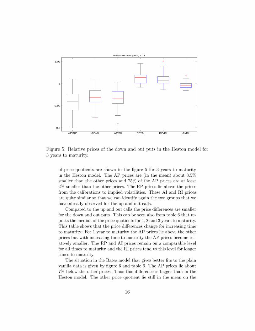
down and out puts, T=3

Figure 5: Relative prices of the down and out puts in the Heston model for3 years to maturity.

of price quotients are shown in the figure 5 for 3 years to maturityin the Heston model. The AP prices are (in the mean) about 3.5%smaller than the other prices and 75% of the AP prices are at least2% smaller than the other prices. The RP prices lie above the pricesfrom the calibrations to implied volatilities. These AI and RI pricesare quite similar so that we can identify again the two groups that wehave already observed for the up and out calls.

Compared to the up and out calls the price differences are smallerfor the down and out puts. This can be seen also from table 6 that re-ports the median of the price quotients for 1, 2 and 3 years to maturity.This table shows that the price differences change for increasing timeto maturity: For 1 year to maturity the AP prices lie above the otherprices but with increasing time to maturity the AP prices become rel-atively smaller. The RP and AI prices remain on a comparable levelfor all times to maturity and the RI prices tend to this level for longertimes to maturity.

The situation in the Bates model that gives better fits to the plainvanilla data is given by figure 6 and table 6. The AP prices lie about7% below the other prices. Thus this difference is bigger than in theHeston model. The other price quotient lie still in the mean on the

16


T = 2 0.983 0.994 0.984 1.011 0.997 0.986T = 3 0.960 0.969 0.968 1.014 1.008 0.996

Bates T = 1 1.021 1.012 1.019 1.004 1.006 0.998T = 2 0.968 0.975 0.966 1.031 1.022 0.990T = 3 0.922 0.935 0.931 1.026 1.022 0.995

Table 6: Median of price quotients of down and out puts.


0.7

0.75

0.8

0.85

0.9

0.95

1

1.05

1.1

1.15


Figure 6: Relative prices of the down and out puts in the Bates model for 3years to maturity.

17

same level but the their variance has grown compared to the Hestonmodel.

The situation for the barrier options can be summarized as follows:The AP prices differ significantly from the other prices for both barrieroptions. While the AP prices are higher for up and out calls they arelower for down and out puts relatively to the other prices. In thissense the situation is symmetrical. The differences become bigger forlonger times to maturity and the better fit of the Bates model doesnot lead to smaller price differences.

4.3 Cliquet Options

We consider cliquet options with prices

exp(−rT ) E[H]

where the payoff H is given by

Hdef= min(cg,max[fg,

N∑i=1

min{cil,max(f il ,Sti − Sti−1

Sti−1

)}]).

Here cg (fg) is a global cap (floor) and cig (f ig) is a local cap (floor) for

the period [ti−1, ti].We consider three periods with ti = T

3 i (i = 0, . . . , 3) and the capsand floors are given by

cg = ∞fg = 0

cil = 0.08, i = 1, 2, 3

f il = −0.08, i = 1, 2, 3

Cliquet options have many parameters. Hence, this specification can-not give representative picture of all the traded cliquets. But thesecaps and floors are typical because the option holder cannot loosemoney and the returns is bounded above only by the local returnbounds.

Cliquet options pay out basically the sum of the returns Ridef=

Sti−Sti−1

Sti−1. In order to reduce risk local and global floors f are intro-

duced for the returns R. In the same way the returns are boundedabove by local and global caps c.

18

The distributions of the six time series of price quotients for cliquetoptions are described in figure 7 for 3 years to maturity in the Hestonmodel. The differences are smaller than in the case of the barrieroptions. The AP prices lie above the other prices but the differenceis significant only for the AP and RP prices. The differences betweenthe other prices is also small. Thus, we cannot recognize directly fromthis figure the two groups that we identified for the barrier options.

Table 7 that reports the median price differences for 1, 2 and 3years to maturity gives some insight into this situation: The AP pricesare about 2% smaller than the other prices for 1 year to maturity.With increasing time to maturity the AP prices grow relatively andare about 1.5% higher than the other prices for 3 years to maturity.As table 7 confirms the other prices remain relatively constant fordifferent times to maturity. Thus there are again the two groups thatwe have identified for the barrier options: The changing AP prices onthe one hand and the constant other prices on the other hand.

The relative prices of the cliquet options in the Bates model arepresented in figure 8 for 3 years to maturity. Here we see that the APprices are about 7% smaller than the other prices. The RP prices lieabout 2% under the AI prices that are 3% higher than the RI prices.The RP and RI prices are similar. Thus, there are quite big differencesfor the cliquet options in the Bates model. Moreover, the variance islarger relative to the Heston model. Table 7 describes the situation ofdifferent times to maturity and shows that the AP prices grow rela-tively with increasing time to maturity while the other prices remainrelatively constant for different times to maturity.

Comparing the results for the two barrier options and the cliquetswe see in all cases two groups, the AP prices and the other prices. TheAP prices differ a lot from the other prices and in addition changerelatively for different times to maturity. Moreover, the variance ofthe price quotient with AP prices is bigger in general than for theother price quotients. The other group of RP, AI and RI prices showssimilar prices and small variances. The Bates model that gives betterfits has higher price differences (with higher variances).

19


T = 2 1.002 0.991 1.000 0.989 0.998 1.010T = 3 1.022 1.008 1.014 0.987 0.992 1.005

Bates T = 1 0.917 0.899 0.917 0.987 1.005 1.024T = 2 0.931 0.903 0.923 0.980 0.999 1.029T = 3 0.946 0.912 0.933 0.976 0.995 1.029

Table 7: Median of price quotients of cliquet options.


0.96

0.98

1

1.02

1.04

1.06

cliquet options, T=3

Figure 7: Relative prices of the cliquet options in the Heston model for 3years to maturity.

20


0.7

0.8

0.9

1

1.1

1.2

1.3


Figure 8: Relative prices of the cliquet options in the Bates model for 3 yearsto maturity.

5 Model risk

In the last section, we have described the price differences that resultfrom the calibration w.r.t. the four error functionals. In this sectionwe consider model risk, consider its relation to calibration risk andcompare our results with the findings of Schoutens et al. (2004). Modelrisk is generally understood as the risk of wrong prices because a wrongparametric model has been chosen for the stochastic process of theunderlying.

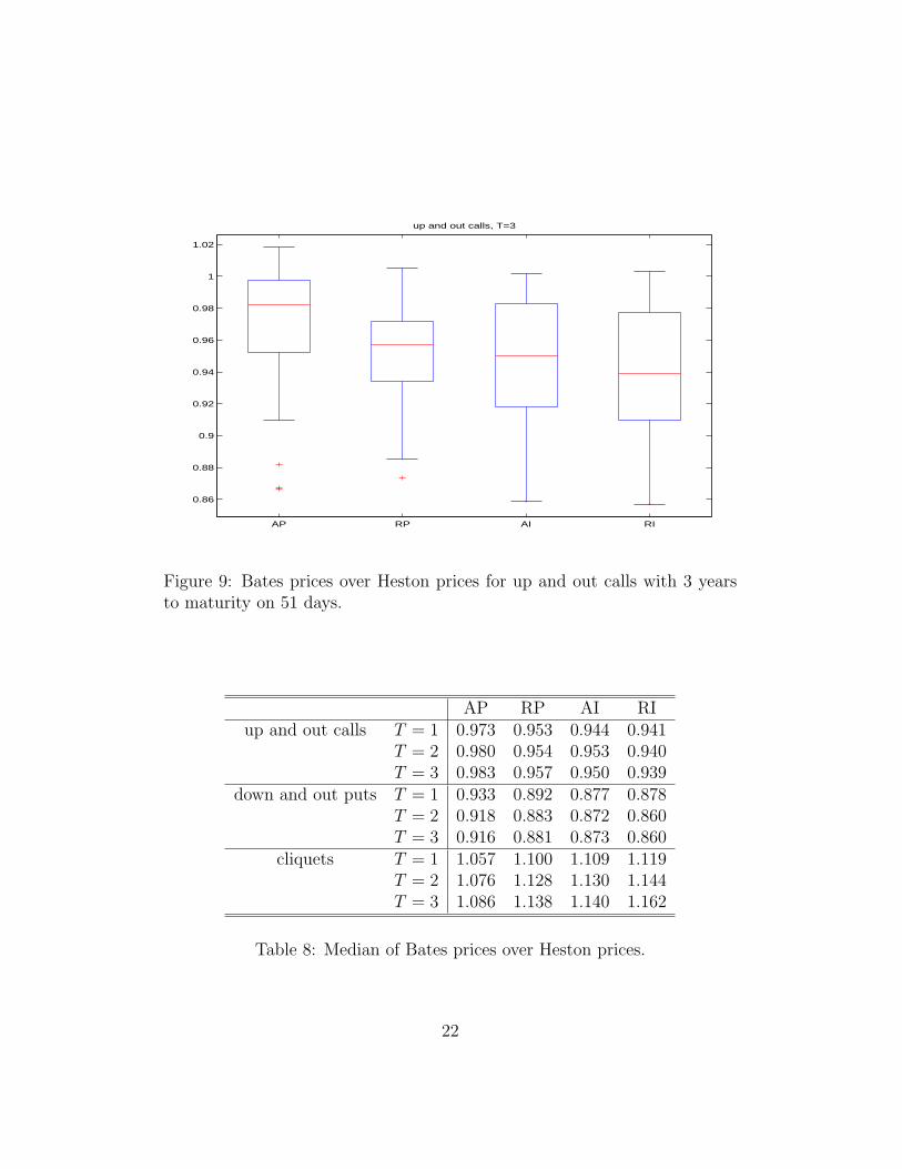
In order to analyze this model risk for the two stochastic volatilitymodels, we consider the quotients of the prices of the exotic optionsin the Bates model and the corresponding prices in the Heston model.The distribution of these quotients for up and out calls with 3 years tomaturity is described by the figure 9. The prices in the Bates modellie below the prices in the Heston model for all four error functionals:The difference varies between 2% for the AP prices and 6% for the RIprices. Thus model risk is not independent of the calibration method,i.e. calibration risk. The results for smaller times to maturity aregiven in table 8. The table suggests that model risk does not changesignificantly for different times to maturity.

21

AP RP AI RI

0.86

0.88

0.9

0.92

0.94

0.96

0.98

1

1.02


Figure 9: Bates prices over Heston prices for up and out calls with 3 yearsto maturity on 51 days.

AP RP AI RIup and out calls T = 1 0.973 0.953 0.944 0.941

T = 2 0.980 0.954 0.953 0.940T = 3 0.983 0.957 0.950 0.939

down and out puts T = 1 0.933 0.892 0.877 0.878T = 2 0.918 0.883 0.872 0.860T = 3 0.916 0.881 0.873 0.860

cliquets T = 1 1.057 1.100 1.109 1.119T = 2 1.076 1.128 1.130 1.144T = 3 1.086 1.138 1.140 1.162

Table 8: Median of Bates prices over Heston prices.

22

AP RP AI RI

0.8

0.85

0.9

0.95

1

1.05

1.1


Figure 10: Bates prices over Heston prices for down and out puts with 3years to maturity on 51 days.

The model risk of down and out puts is shown in figure 10 for 3years to maturity. The prices in the Bates model lie below the pricesin the Heston model for all error functionals. Compared to the upand out calls the model risk is bigger for the down and out puts: Itvaries between 9% for AP prices and 14% for RI prices. But again weobserve the highest difference for RI prices and the smallest for APprices. Moreover, the variance is bigger than for the up and out calls.Table 8 that gives the results for smaller times to maturity suggeststhat the model risk becomes smaller for shorter times to maturity.

Finally, we consider the model risk of cliquet options in figure 11.For these options the Bates prices lie above the corresponding Hestonprices for all calibration methods. The smallest price difference thatappears for the AP prices is about 8% while the biggest difference of16% have the RI prices. Table 8 shows again smaller price differencesfor shorter times to maturity.

The model risk between the Heston and the Bates model can be de-scribed for barrier and cliquet options as follows: Model risk measuredby the price differences in the two models increasing for longer times

23

AP RP AI RI

0.8

0.85

0.9

0.95

1

1.05

1.1

1.15

1.2

1.25

1.3


Figure 11: Bates prices over Heston prices for cliquet options with 3 years tomaturity on 51 days.

to maturity. Moreover, it is ordered w.r.t. the calibration method.The calibration w.r.t. implied volatilities leads to bigger price differ-ences as calibration w.r.t. prices. The model risk is smallest for APcalibration and bigger for RP calibration. It is even bigger for theAI calibration and the price differences are the biggest for RI cali-brations. This emphasizes once more the importance of the impliedvolatility surfaces and their calibration. Moreover, model risk differsacross option types.

Schoutens et al. (2004) consider up and out calls (with strike equalto spot) and cliquet options with 3 years to maturity. For a barrier50% above the spot, they find a model risk for the up and out callsof about 14%. For the cliquet options Schoutens et al. do not find asignificant model risk. These results do not correspond in every respectto our AP results. There may be several reasons for these differentresults: While we look at a time series of 51 implied volatility surfacesthey focus one one day. They have analyzed the EuroStoxx50 and weuse DAX data.

24

6 Conclusion

We have looked at the popular stochastic volatility model of Hestonand analyzed different calibration methods and their impact on thepricing of exotic options. Our analysis was carried out for a time seriesof DAX implied volatility surfaces from April 2003 to March 2004.

We have shown that different ways to measure the error betweenthe model and the market in the calibration routine lead to significantprice differences of exotic options in the sense that these differencesoften exceed the profit margins of the products. We have consideredthe four error measures that are defined by the root mean squarederror of absolute or relative differences of prices or implied volatilities.Among these measures we have identified two groups: Calibrationsw.r.t. relative prices, absolute implied volatilities or relative impliedvolatilities lead to similar prices of exotic options. Calibrations w.r.t.absolute prices imply exotics prices that are quite different from theprices of the first group. The price differences increase for longer timesto maturity. Moreover, the differences do not decrease in the Batesmodel although it is an extension of the Heston model with similarqualitative features and a better fit to plain vanilla data. The pricedifferences of exotic options differ also across option types and arebigger for barrier options than for cliquets.

Moreover, we have looked at the model risk for these two optionpricing models. Model risk and calibration risk are not independentbecause model risk is lowest for calibrations w.r.t. absolute pricesand highest for calibrations w.r.t. relative implied volatilities. As thisholds for all considered options model risk seems to be ordered w.r.t.the error measure used in the calibration.

As model risk is bigger than calibration risk calibrations shouldbe carried out w.r.t. absolute prices if the choice of an appropriatemodel is unclear. But if a model has already been chosen we suggestto measure the error between the model and the market in terms of(relative) implied volatilities because this error measure reflects bestthe characteristics of the model that are essential for exotic options.Moreover, we have demonstrated that this choice leads to good cal-ibrations (e.g. relatively good fits and stable parameters). We havealso shown that the resulting prices of exotic options often lie in themiddle of the prices from the other calibrations and have the small-est variance. Our results underline the importance of the impliedvolatility surface and suggest that one should measure the error in the

25

calibration in terms of implied volatilities.

References

Bates, D. (1996). Jump and Stochastic Volatility: Exchange RateProcesses Implicit in Deutsche Mark Options, Review of Finan-cial Studies 9: 69-107.

Carr, P. & Madan, D. (1999). Option valuation using the fast Fouriertransform, Journal of Computational Finance 2: 61–73.

Cont, R. (2005 ). Model uncertainty and its impact on the pricing ofderivative instruments, to appear in Mathematical Finance.

Cont, R. & Tankov, P. (2004). Financial Modelling With JumpProcesses, Chapman & Hall/CRC.

Glasserman, P. (2004). Monte Carlo Methods in Financial Engineer-ing, Springer, New York.

Heston, S. (1993). A closed-form solution for options with stochasticvolatility with applications to bond and currency options, Reviewof Financial Studies 6: 327-343.

Mikhailov, S. & Nogel, U. (2003). Heston’s stochastic volatility model.Implementation, calibration and some extensions, Wilmott mag-azine, July 2003.

Schoutens, W., Simons, E. & Tistaert, J. (2004). A Perfect Calibra-tion! Now What? Wilmott magazine, March 2004.

26

ξ η θ ρ V0

AP 0.87 0.07 0.34 -0.82 0.07(0.48) (0.02) (0.08) (0.08) (0.02)

RP 1.38 0.07 0.44 -0.74 0.08(0.35) (0.02) (0.06) (0.03) (0.02)

AI 1.32 0.07 0.43 -0.77 0.08(0.40) (0.02) (0.06) (0.04) (0.02)

RI 1.20 0.07 0.41 -0.75 0.08(0.35) (0.02) (0.06) (0.05) (0.02)

Table 9: Mean parameters (std.) in the Heston model for 51 days.

ξ η θ ρ V0 λ k δAP 0.92 0.07 0.33 -0.94 0.07 0.33 0.07 0.08

(0.50) (0.02) (0.08) (0.07) (0.02) (0.21) (0.03) (0.06)RP 1.56 0.07 0.45 -0.89 0.08 0.54 0.05 0.08

(0.47) (0.02) (0.07) (0.07) (0.02) (0.23) (0.03) (0.06)AI 1.43 0.07 0.43 -0.95 0.07 0.50 0.06 0.09

(0.44) (0.02) (0.06) (0.06) (0.02) (0.22) (0.03) (0.04)RI 1.36 0.07 0.41 -0.93 0.07 0.52 0.05 0.08

(0.44) (0.02) (0.07) (0.09) (0.02) (0.26) (0.04) (0.08)

Table 10: Mean parameters (std.) in the Bates model for 51 days.

27

SFB 649 Discussion Paper Series 2006

For a complete list of Discussion Papers published by the SFB 649, please visit http://sfb649.wiwi.hu-berlin.de.

001 "Calibration Risk for Exotic Options" by Kai Detlefsen and Wolfgang K. Härdle, January 2006.

SFB 649, Spandauer Straße 1, D-10178 Berlin http://sfb649.wiwi.hu-berlin.de

This research was supported by the Deutsche

Forschungsgemeinschaft through the SFB 649 "Economic Risk".

calibration risk for exotic options - econstor

Documents