calibrating passive acoustic monitoring: correcting...

Calibrating passive acoustic monitoring:Correcting humpback whale call detections forsite-specific and time-dependent environmental

characteristicsTyler A. Helble,a) Gerald L. D’Spain, Greg S. Campbell, and

John A. HildebrandScripps Institution of Oceanography, University of California at San Diego, La Jolla,

California [email protected], [email protected], [email protected], [email protected]

Abstract: This paper demonstrates the importance of accounting forenvironmental effects on passive underwater acoustic monitoringresults. The situation considered is the reduction in shipping off theCalifornia coast between 2008–2010 due to the recession and environ-mental legislation. The resulting variations in ocean noise change theprobability of detecting marine mammal vocalizations. An acousticmodel was used to calculate the time-varying probability of detectinghumpback whale vocalizations under best-guess environmental condi-tions and varying noise. The uncorrected call counts suggest a diel pat-tern and an increase in calling over a two-year period; the corrected callcounts show minimal evidence of these features.VC 2013 Acoustical Society of AmericaPACS numbers: 43.30.Sf, 43.60.Cg, 43.80.Ka [AL]Date Received: March 28, 2013 Date Accepted: August 21, 2013

1. Introduction

Passive acoustic monitoring is an important tool for understanding marine mammal ecol-ogy and behavior. When studying an acoustic record containing marine mammal vocaliza-tions, the received signal can be greatly influenced by the environment in which the soundis transmitted. The ocean bottom properties, bathymetry, and temporally varying soundspeed act to distort and reduce the energy of the original waveform produced by the ma-rine mammal. In addition, constantly varying ocean noise further influences the detectabil-ity of the calls. This ever-changing acoustic environment creates difficulties when compar-ing marine mammal recordings between sensors, or at the same sensor over time.

One way to correct for temporal and spatial variations in detectability due toenvironmental effects can be obtained from the expression for estimating the spatialdensity of marine mammals from passive acoustic recordings: Eq. (3) of Marqueset al.1 The corrected call counts in Eq. (3) are

N c � nc1� c

P; (1)

where nc is the number of detections (uncorrected call count) in the data, c is the prob-ability of false detection, and P is the probability of detection. In the case wherehuman analysts scan the detection outputs generated by an automated detection algo-rithm to eliminate false detections (i.e., c ¼ 0) as is done with the data presented inthis paper, the calibration factor is the estimated probability of detection, P. Helbleet al.2 demonstrated that P can change by factors >10 between sensors at different

a)Author to whom correspondence should be addressed.

EL400 J. Acoust. Soc. Am. 134 (5), November 2013 VC 2013 Acoustical Society of America

Helble et al.: JASA Express Letters [http://dx.doi.org/10.1121/1.4822319] Published Online 10 October 2013

http://crossmark.crossref.org/dialog/?doi=10.1121/1.4822319&domain=pdf&date_stamp=2013-10-10

locations or at the same sensor over time. At some sites, P has an exponential depend-ence on ocean noise level and, hence, a seemingly modest change in noise, itself insig-nificant in the high dynamic range spectrograms commonly used to detect vocaliza-tions, can nonetheless greatly skew the counts of calling activity. To illustrate theinfluence that the ocean environment has on the detection of marine mammal vocaliza-tions, two single hydrophone datasets simultaneously recorded over a two-year periodusing high-frequency acoustic recording packages (HARP)3 were analyzed for hump-back whale (Megaptera novaeangliae) vocalizations. Humpback vocalizations consist ofa sequence of discrete sound elements called units that are separated by silence.4 Therecorded detection counts (number of detected units) were corrected to account for theinfluence of environmental properties using the numerically derived probability ofdetection. The resulting environmentally calibrated datasets provide a more validapproach to examining both short-term and long-term calling trends of the biologicalsources themselves. The two sites are located off the coast of California as shown inFig. 1, which also illustrates shipping traffic for the region using the ship AutomaticIdentification System (AIS).5 Site SBC (34.2754�, �120.0238�) is located in the center ofthe Santa Barbara Channel, and site SR (36.3127�, �122.3926�) is located on Sur Ridge,a bathymetric feature 45 km southwest of Monterey. Data recording covers the periodfrom January 2008 to January 2010, during which a decrease in shipping noise occurredat both locations due to a downturn in the world economy, coupled with the implementa-tion of an air-quality improvement rule on 1 July 2009, by the California Air ResourcesBoard (CARB). McKenna et al.6 discovered that these events in combination reducedthe monthly average ocean noise level by 12 dB re 1 lPa2/Hz in the 1-Hz wide band at40 Hz and by 9 dB re 1 lPa2/Hz in the 1-Hz wide band at 90 Hz over a period from 2007to 2010 at site SBC. Additionally, shipping traffic creates variability in the recorded noiselevels at both sites on daily time scales. Ship AIS data has been used in combination withocean noise recordings to reveal a correlation in shipping density with ocean noise, whichpeaks during the morning and evening hours, and remains lowest during nighttime hoursat site SBC.7 The changing ocean noise characteristics at these two sites create significantchanges in P on both short-term and long-term time scales.

2. Methods

The methods presented in this paper rely heavily on the modeling results and analysismethods described in Helble et al.2 The paper describes how values of P were determinedfor both site SBC and site SR over a range of potential environmental conditions includ-ing ocean noise levels, sound speed profiles, bathymetry, and ocean bottom characteris-tics. Additionally, the uncertainties in P over a range of likely environmental conditionswere determined, and the results were validated by means of model/data comparisons.The approach in Helble et al.2 uses a full wavefield acoustic propagation model[“CRAM,” based on the range-dependent acoustic model (RAM)8] to simulate the prop-agation of humpback call units from source to receiver, in amplitude and phase as a func-tion of frequency. The model simulated calls originating from geographical locationsevenly spaced on a lattice with 20 arc-sec spacing, bounded by a 20 km radial distancefrom the HARP, at 20 m depth. The simulated received humpback units for each sitewere added to time-varying noise recorded from each site and the generalized power-lawdetector9 was used to process the combined waveform. Resulting probability of detectionmaps were created as a function of latitude and longitude for the areas surrounding eachHARP. From these maps, the average probability of detection for a 20 km radial areawas determined for a full range of noise conditions, yielding probability of detection ver-sus noise curves for both site SBC and site SR.

Sound speed profiles were obtained from oceanographic casts taken near theHARP recording packages. Monthly variations in sound speed profiles changed esti-mates in P by no more than 20% for site SBC and 10% at site SR. In contrast,changes in sound speed profile that occur between summer and winter profile types canlead to significantly greater changes in P at site SBC (only slightly higher than 10%


J. Acoust. Soc. Am. 134 (5), November 2013 Helble et al.: Calibrating passive acoustic call detections EL401

change at site SR).2 Therefore, updating the input sound speed profile twice annuallycaptured this seasonal variability in the modeling.

Values of P were then used to normalize the counts of real humpback detec-tions (nc) recorded on the HARP sensors at site SBC and site SR for 2008 and 2009.This normalization yielded the estimated number of call units that actually occurredwithin the 20 km radial area surrounding the HARP ðN cÞ, assuming a uniform distri-bution of calling animals in the area monitored. In order to satisfy this assumption,detected units were tabulated in weekly increments. Model/data comparisons fromHelble et al.2 indicate this assumption likely is true at least on monthly time scales forboth sites SR and SBC. The resulting normalized call counts were provided in numberof units per km2 per week. On shorter time scales, the calling animals cannot beassumed to be uniformly distributed. However, comparing unnormalized call countswith variations in P on shorter time scales is important to gain an understanding ofthe correlation between detection counts and variations in ocean noise levels, and thisanalysis was carried through for site SBC (discussed in Sec. 3).

3. Results

Ocean noise levels (in units of dB re 1 lPa2) were obtained by integrating the spectraldensity (in units of dB re 1 lPa2/Hz) over the 150–1800 Hz bands. Time periods withdetected humpback vocalizations or other obvious biological sources were omittedfrom the noise measurements. Ocean noise levels averaged over consecutive 75-s peri-ods between 2008–2009 varied by up to 35 dB at both locations (Fig. 2 and 75–110 dBre 1 lPa2 in the 150–1800 Hz band). The seven-day running means of the noise (greencurves) are better able to reveal long-term changes in the noise. The decrease at SBCof �5 dB in the integrated spectral density of the 150–1800 Hz band over the course ofthe deployment is consistent with the downward trend described by McKenna et al.6

at 50 Hz and at 90 Hz. The decrease in ocean noise occurs with the onset of the GreatRecession, which significantly reduced maritime trade.6 An additional reduction inocean noise at SBC occurred in the 150–1800 Hz band after July 1, 2009, with theenforcement of the CARB air quality improvement rule, again consistent with theresults at 40 Hz and 90 Hz. It resulted in a diversion of much of the shipping traffic totransit lanes outside of the channel. Similar results can be seen for site SR; a significantdrop occurs in both ocean noise levels and in the variance of ocean noise when

Fig. 1. Map of coastal California showing the two HARP locations: site SBC and site SR (stars). Ship trafficfrom the AIS is shown for the region. The color scale indicates the number of recorded unique transits within a1 km2 area from October 2009–October 2010. Yellow and orange regions indicate 76–500 total transits, redregions indicate 501–1250 total transits, and purple regions indicate greater than 1251 transits. Note that shiptraffic is shown after the enforcement of CARB law, as indicated by greater shipping traffic outside the SantaBarbara Channel.


EL402 J. Acoust. Soc. Am. 134 (5), November 2013 Helble et al.: Calibrating passive acoustic call detections

comparing the Aug–Dec 2008 levels with those of Aug–Dec 2009. The time periodfrom Feb–Jul 2008 cannot be directly compared to Feb–Jul 2009 because the sensorduring the former time period was located 10 km southwest of the ridge, in deeperwater. The black curve for site SR in Fig. 2 indicates the seven-day average noise levelwhen each noise estimate used in the average is made from the 75-s time period sur-rounding each detected humpback unit. When averaging the noise estimates this way,the resulting noise level generally falls below the running mean noise level for the sametime period (i.e., the black curve generally falls below the green curve) because anincreasing number of units is detected during periods of lower noise. This discrepancyindicates the need to obtain noise estimates during the periods of marine mammalvocalization detections; using a simple running-mean noise average does not properlyrepresent the noise environment in which the calls are detected.

Figure 3 shows ocean noise levels for site SBC for a one week period in May2008 (upper plot), the related values of P (middle plot), and the uncorrected numberof units detected per hour over the same period (lower plot). Examination of the lowerplot by itself would indicate a strong diel cycle to the humpback calling activity, withsignificantly more calls occurring during nighttime. However, inspection of P indicatesa significant diel cycle in the likelihood of detecting humpback units. This change in Pcould account for much of the diel signal found in the humpback calling pattern forthis period. While nearby passages of ships are easily identified (short duration spikesin the upper plot), smaller noise variations centered near 80 dB re 1 lPa2 are difficultto notice if detections are manually marked from a spectrogram. When ocean noiselevels at site SBC drop from 80 dB re 1 lPa2 to 75 dB re 1 lPa2, P increases from 0.1to 0.65 (see Fig. 9 of Helble et al.2). The reason is that calls from a large area thatwere buried in noise at higher noise levels become detectible with the decrease in noise.This observation illustrates the importance of correcting for subtle variations in noiseat this site (in contrast, large spikes in noise that occur in a high noise environmenthave little effect reducing P because P is already low). Changes of only a few decibelsin noise level can have substantially different effects on the change in P depending on

Fig. 2. Ocean noise levels in the 150–1800 Hz band over the 2008–2009 period at site SBC (upper) and SR(lower). The gray curves indicate the noise levels averaged over 75 s increments, the green curves are the runningmean with a seven-day window, and the black curve (site SR only) is a plot of the average noise levels in aseven-day window measured at the times adjacent to each detected humpback unit. White spaces indicate peri-ods with no data. The blue vertical lines mark the start of enforcement of CARB law.



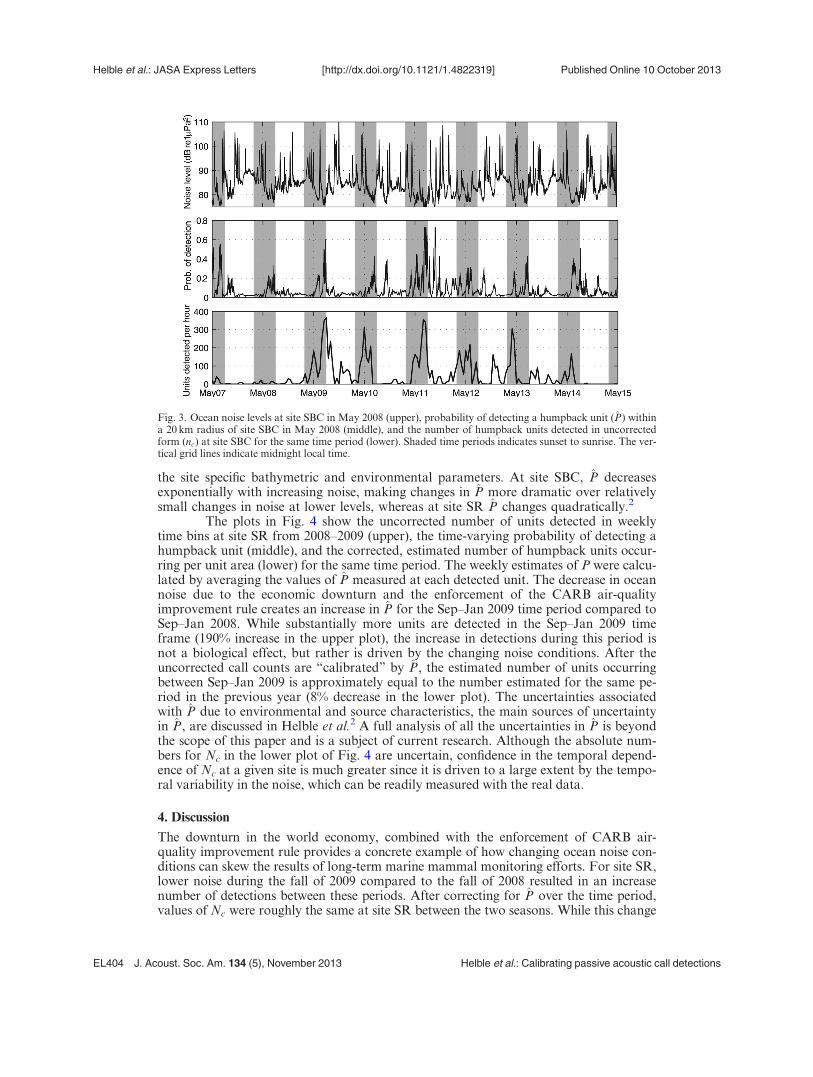
the site specific bathymetric and environmental parameters. At site SBC, P decreasesexponentially with increasing noise, making changes in P more dramatic over relativelysmall changes in noise at lower levels, whereas at site SR P changes quadratically.2

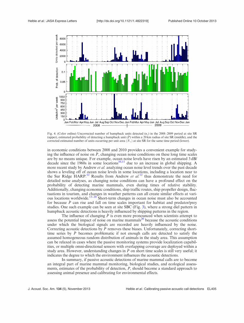
The plots in Fig. 4 show the uncorrected number of units detected in weeklytime bins at site SR from 2008–2009 (upper), the time-varying probability of detecting ahumpback unit (middle), and the corrected, estimated number of humpback units occur-ring per unit area (lower) for the same time period. The weekly estimates of P were calcu-lated by averaging the values of P measured at each detected unit. The decrease in oceannoise due to the economic downturn and the enforcement of the CARB air-qualityimprovement rule creates an increase in P for the Sep–Jan 2009 time period compared toSep–Jan 2008. While substantially more units are detected in the Sep–Jan 2009 timeframe (190% increase in the upper plot), the increase in detections during this period isnot a biological effect, but rather is driven by the changing noise conditions. After theuncorrected call counts are “calibrated” by P, the estimated number of units occurringbetween Sep–Jan 2009 is approximately equal to the number estimated for the same pe-riod in the previous year (8% decrease in the lower plot). The uncertainties associatedwith P due to environmental and source characteristics, the main sources of uncertaintyin P, are discussed in Helble et al.2 A full analysis of all the uncertainties in P is beyondthe scope of this paper and is a subject of current research. Although the absolute num-bers for Nc in the lower plot of Fig. 4 are uncertain, confidence in the temporal depend-ence of Nc at a given site is much greater since it is driven to a large extent by the tempo-ral variability in the noise, which can be readily measured with the real data.

4. Discussion

The downturn in the world economy, combined with the enforcement of CARB air-quality improvement rule provides a concrete example of how changing ocean noise con-ditions can skew the results of long-term marine mammal monitoring efforts. For site SR,lower noise during the fall of 2009 compared to the fall of 2008 resulted in an increasenumber of detections between these periods. After correcting for P over the time period,values of Nc were roughly the same at site SR between the two seasons. While this change

Fig. 3. Ocean noise levels at site SBC in May 2008 (upper), probability of detecting a humpback unit (P) withina 20 km radius of site SBC in May 2008 (middle), and the number of humpback units detected in uncorrectedform (nc) at site SBC for the same time period (lower). Shaded time periods indicates sunset to sunrise. The ver-tical grid lines indicate midnight local time.



in economic conditions between 2008 and 2010 provides a convenient example for study-ing the influence of noise on P, changing ocean noise conditions on these long time scalesare by no means unique. For example, ocean noise levels have risen by an estimated 3 dB/decade since the 1960s in some locations10,11 due to an increase in global shipping. Amore recent study by Andrew et al. analyzing ocean noise level trends over the past decadeshows a leveling off of ocean noise levels in some locations, including a location near tothe Sur Ridge HARP.12 Results from Andrew et al.12 thus demonstrate the need fordetailed noise analyses, as changing noise conditions can have a profound effect on theprobability of detecting marine mammals, even during times of relative stability.Additionally, changing economic conditions, ship traffic routes, ship propeller design, fluc-tuations in tourism, and changes in weather patterns can all create similar effects at vari-ous locations worldwide.13–20 Short-term changes in ocean noise must also be accountedfor because P can rise and fall on time scales important for habitat and predator/preystudies. One such example can be seen at site SBC (Fig. 3), where a strong diel pattern inhumpback acoustic detections is heavily influenced by shipping patterns in the region.

The influence of changing P is even more pronounced when scientists attempt toassess the potential impact of noise on marine mammals20 because the acoustic conditionsunder which the biological signals are recorded are heavily influenced by the noise.Correcting acoustic detections by P removes these biases. Unfortunately, correcting short-time series by P becomes problematic if not enough calls are detected to satisfy theassumed homogeneous random distribution of animals in the study area. This assumptioncan be relaxed in cases where the passive monitoring systems provide localization capabil-ities, or multiple omni-directional sensors with overlapping coverage are deployed within astudy area. However, understanding changes in P on short time scales is still very useful; itindicates the degree to which the environment influences the acoustic detections.

In summary, if passive acoustic detections of marine mammal calls are to becomean integral part of marine mammal monitoring, biological studies, and ecological assess-ments, estimates of the probability of detection, P, should become a standard approach toassessing animal presence and calibrating for environmental effects.

Fig. 4. (Color online) Uncorrected number of humpback units detected (nc) in the 2008–2009 period at site SR(upper), estimated probability of detecting a humpback unit (P) within a 20 km radius of site SR (middle), and thecorrected estimated number of units occurring per unit area ðN cÞ at site SR for the same time period (lower).



Acknowledgments

The authors are extremely grateful to Professor Glenn Ierley, Dr. Megan McKenna, andAmanda Debich, all at the Scripps Institution of Oceanography, for their support of thisresearch. Special thanks to Sean Wiggins and the entire Scripps Whale Acoustics Laboratoryfor providing thousands of hours of high quality acoustic recordings. Richard Campbell andKevin Heaney of Ocean Acoustical Services and Instrumentation Systems, Inc. wrote theacoustic propagation code CRAM, based on Mike Collins’ RAM parabolic equation code.T.A.H. would like to thank the Department of Defense Science, Mathematics, and Researchfor Transformation (SMART) Scholarship program and the Space and Naval Warfare(SPAWAR) Systems Command Center Pacific In-House Laboratory Independent Researchprogram. Work was also supported by the Office of Naval Research, Code 322 (MBB), theChief of Naval Operations N45, and the Naval Postgraduate School.

References and links1T. Marques, L. Thomas, J. Ward, N. DiMarzio, and P. Tyack, “Estimating cetacean population densityusing fixed passive acoustic sensors: An example with Blainville’s beaked whales,” J. Acoust. Soc. Am.125, 1982–1994 (2009).

2T. Helble, G. D’Spain, J. Hildebrand, G. Campbell, R. Campbell, and K. Heaney, “Site specificprobability of passive acoustic detection of humpback whale calls from single fixed hydrophones,”J. Acoust. Soc. Am. 134, 2556–2570 (2013).

3S. Wiggins, “Autonomous Acoustic Recording Packages (ARPs) for long-term monitoring of whalesounds,” Marine Technol. Soc. J. 37, 13–22 (2003).

4R. Payne and S. McVay, “Songs of humpback whales,” Science 173, 585–597 (1971).5Digital Coast: NOAA Coastal Services Center, “2009–2010 commercial vessel density (October - AIS),”2013, available at URL http://www.marinecadastre.gov/ (Last viewed 7/11/2013).

6M. McKenna, S. Katz, S. Wiggins, D. Ross, and J. Hildebrand, “A quieting ocean: Unintendedconsequence of a fluctuating economy,” J. Acoust. Soc. Am. 132, EL169–EL175 (2012).

7M. McKenna, M. Soldevilla, E. Oleson, S. Wiggins, and J. Hildebrand, “Increased underwater noiselevels in the Santa Barbara Channel from commercial ship traffic and its potential impact on Blue whales(Balaenoptera musculus),” in Proceedings of the Seventh California Islands Symposium, edited by C. C.Damiani and D. K. Garcelon (Institute for Wildlife Studies, Arcata, CA, 2009), pp. 141–149.

8M. Collins, User’s Guide for RAM Versions 1.0 and 1.0p (Naval Research Laboratory, Washington, DC,2002), available at URL http://www.siplab.fct.ualg.pt/models/ram/manual.pdf (Last viewed 03/02/2013).

9T. Helble, G. Ierley, G. D’Spain, M. Roch, and J. Hildebrand, “A generalized power-law detection algo-rithm for humpback whale vocalizations,” J. Acoust. Soc. Am. 131, 2682–2699 (2012).

10R. Andrew, B. Howe, J. Mercer, and M. Dzieciuch, “Ocean ambient sound: Comparing the 1960s withthe 1990s for a receiver off the California coast,” ARLO 3, 65–70 (2002).

11D. Ross, “On ocean underwater ambient noise,” Inst. Acoust. Bull. 18, 5–8 (1993).12R. Andrew, B. Howe, and J. Mercer, “Long-time trends in ship traffic noise for four sites off the North

American West Coast,” J. Acoust. Soc. Am. 129, 642–651 (2012).13G. Wenz, “Review of underwater acoustics research: Noise,” J. Acoust. Soc. Am. 51, 1010–1024 (1972).14P. Kaluza, A. K€olzsch, M. Gastner, and B. Blasius, “The complex network of global cargo ship

movements,” J. R. Soc., Interface 7, 1093–1103 (2010).15K. Matveev, “Effect of drag-reducing air lubrication on underwater noise radiation from ship hulls,”

J. Vibr. Acoust. 127, 420–422 (2005).16P. Arveson and D. Vendittis, “Radiated noise characteristics of a modern cargo ship,” J. Acoust. Soc.

Am. 107, 118–129 (2000).17M. McKenna, D. Ross, S. Wiggins, and J. Hildebrand, “Underwater radiated noise from modern

commercial ships,” J. Acoust. Soc. Am. 131, 92–103 (2012).18V. Knudsen, R. Alford, and J. Emling, “Underwater ambient noise,” J. Mar. Res. 7, 410–429 (1948).19G. Wenz, “Acoustic ambient noise in the ocean: Spectra and sources,” J. Acoust. Soc. Am. 34,

1936–1956 (1962).20National Research Council, Ocean Noise and Marine Mammals (National Academies, Washington, DC,

2003), pp. 83–132.



http://www.marinecadastre.gov/

http://www.siplab.fct.ualg.pt/models/ram/manual.pdf

calibrating passive acoustic monitoring: correcting...

Documents