calculus before newton and leibniz - …shodhganga.inflibnet.ac.in/bitstream/10603/50848/8/08...of...

Calculus before Newton and Leibniz 13

CHAPTER – II

CALCULUS BEFORE NEWTON AND LEIBNIZ

2.1: INTRODUCTION

The history of Greek mathematics begins in the 6th century B.C.

Historians traditionally place the beginning of the Greek mathematics proper to

the age of Thales of Miletus (624-548 B.C). Thales and Pythagoras (570BC-)

were the leading mathematicians of this age. Thales who lived in the first half of

the 6th century B.C. proved the following theorems:

1. A diameter of a circle divides it into two equal parts.

2. The base angles of an isosceles triangle are equal.

3. The vertical angles formed by two intersecting straight lines are equal.

4. The angle-side-angle congruence theorem for triangles.

5. Angle in a semi circle is a right angle [26].

Thales and Pythagoras gave an abstract character to Greek mathematics. As

for example the Greek considered the ratio a:b between two numbers a and b as a

relationship between these and not the fraction �� as a single entity. The journey

of factual calculus begins with Pythagoras (569-500 B.C). Though geometry was

the central theme of the Greek mathematics, yet arithmetic was the key attraction

of Pythagoras. Based on this, the early Pythagoreans developed an elementary

theory of proportionality.

2.2: INCOMMENSURABILITY OF LENGTH

Pythagoreans thought that ‘everything is number’. To them, numbers

were positive integrals. They were of the view that our cosmos was created and

governed by understandable and definite numerical principles. The Pythagoreans

were also of the view that the derivation of the multiplicity of creations in the

world from a unique unity is identical to the derivation of numbers from the

numerical unit. They opinined that material world is imitating the mathematical

world.


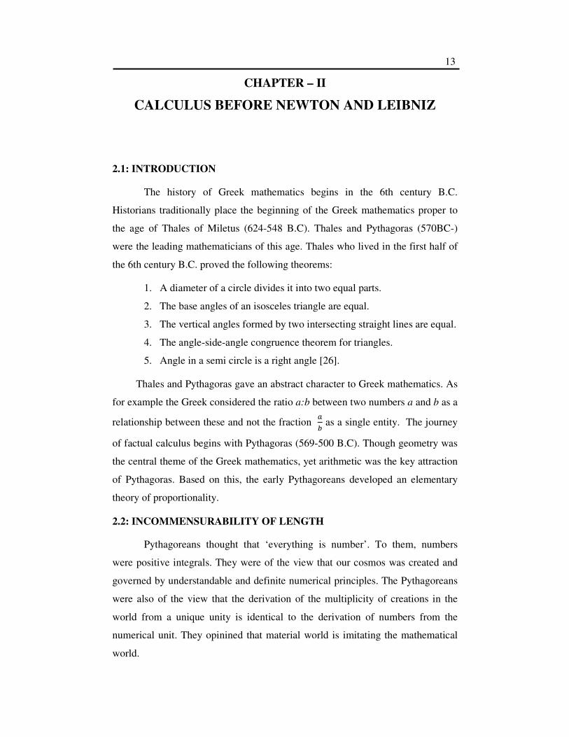
During the later part of 5th century B.C. it was discovered that there exists

incommensurable∗ line segments. Pythagoras thought that every point on a

straight line can be represented by a rational number. Trouble starts when a point

P situated on a line as indicated below to be associated with a number equal to

√2.

The ratio of the edge and the diagonal of a unit square is not equal to the

ratio of two integers. The square on the diagonal of a unit square has area 2

whereas √2 is not commensurable.

Fig. 2.1

222RQPRPQ += � 1� 1�

� 1 1

� 2

PQ = 2

The discovery had raised questions about the idea of measurement and

calculation of geometry as a complete one.

The Pythagorean School around 500 B.C. proved with the help of

‘reductio ad absurdum’ method that there is no rational number whose square is

2. The ‘reductio ad absurdum’ method is that which shows an absurd conclusion

from supposing the theorem is false.

For this reason, the Greeks did not consider geometric magnitudes to be

demonstrated by numbers at all. They did not allow numbers to play the key role

of their mathematics. To them, numbers were discrete integral quantities having

∗ Incommensurable length- The length which cannot be measured as integral multiples of

segments of its length, hence the ratio between their lengths is not equal to the ratio of two

integers.


arithmetic properties. But the geometrical magnitudes were continuous spatial

objects.

2.3: IRRATIONALITY OF √ AND THE INFINITE

The phenomenon of incommensurable lengths showed that geometric

magnitudes have some sort of inherently continuous character which cannot be

avoided. So the Greeks thought that geometric magnitudes cannot be used freely

in algebraic computations.

The notion of irrational numbers such as √2, √3, took a distinguishing

form throughout the Sulva period (600-300 BC) of Hindu mathematics in India.

Though there are nine Sulvasutras on evidence, but only four of them are known

to us. These are (i) Boudhayana (ii) Apastamba (iii) Kaatyayana and (iv)

Maanava.

George Buhler is of the opinion that the slokas 9,10,11 of Boudhayana

Sulvasutra deal with surd numbers dvikarani (√2), trikarani (√3) and

tritiyakarani ( �√� ) through geometrical construction of squares.

Irrationals were introduced in computation around 1200 AD in Europe by

Leonardo of Pisa. To make ground work for irrationals, familiarity of

mathematics of the infinite was mandatory. Till then, no mathematics of the

infinite was exposed as it was thought to be incomprehensible, indescribable and

unthinkable. Modern mathematics says that irrationals can be approximated by

rationales.

2.4: THE INFINITE AND THE GREEK MATHEMATICS

The Infinite and unintelligible to aperion (not limited) that was

propounded by Anaximander of Miletus (610-546 BC) was thought to be present

in the continuous or unbroken magnitudes of geometry. To him, discrete numbers

are unable to represent the infinite. The mathematical “horror of infinity” arose

from the time of Zeno. In those days, popular Pythagorean idea was that a line

consists of points and time is composed of a series of detached moments. Zeno

pointed out the absurdity of “infinite divisibility” of space and time by his famous

paradoxes that involved application of infinite processes to geometry.


The Greeks considered arithmetic and geometry to be essentially distinct.

Their reflection was that the irrational quantities might disprove their philosophy.

This division of mathematics manifests the fundamental division between

finite (arithmetic of whole numbers) and infinite (geometrical continuum).

In respect of √2 Michael Stifel wrote in 1544, “this cannot be a true

number which is of such a nature that it lacks precision. ………, so an irrational

number is not a true number, but lies hidden in a kind of infinity” [42].

2.5: LIMITATION OF PYTHAGOREANS

Numbers to the Pythagoreans are termed today as positive integers. They

could not imagine numbers beyond the positive integers. Even Pythagoreans had

little idea that the theorem of Pythagoras could be relevant in different contexts.

They have no idea that the algebraic equation �� may remind one of

a geometric curve known as circle of radius a, as they developed little

abbreviated symbolism. The interconnection between geometry and algebra was

first observed only by two French mathematicians Pierre de Fermat (1601-1665)

and Rene Descartes (1596-1650).

If the Greek would have emphasized measurement by numbers and not

preferred geometric approach of mathematics by excluding algebraic aspects, the

development of calculus would have been vigorous!

2.6: NICHOLAS OF CUSA AND THE INFINITE

Nicholas of Cusa (1401-1464) was a German cardinal, philosopher and

theologian. The logic of Cusa opened the access for the discussion and debate for

the new field of mathematics of the Infinite. To him, our finite mind is not

competent enough to know the infinite. Nicholas called infinity “absolute”, it

must be perceived in a full and unrestrained sense. The actual infinite would be

known in a transcendental domain through mystical insight only. Mystics called

it Brahman, God, Allah, Tao etc. He believed that there is no comparative

relation between the infinite and the finite. He argued that there cannot be an

opposite to the indescribable infinite. The Absolute Infinite includes all and

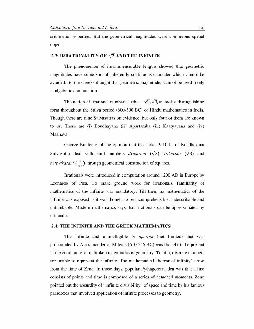
encompasses all. It can be understood by considering an arc of a sequence of

circles of larger and larger diameter which coincides with a line at infinite.


Fig. 2.2

His doctrine of opposites of the finite and the infinite is known as

coincidence of opposites. It is the idea that all kinds of multiplicity in the finite

world become one in the infinite. It was used not only for studying theology or

philosophy, but for mathematics also. For example,

(i) A curve and a straight line are opposites, but if the radius of a circle is

made infinitely long, then its curved circumference coincides with a

straight line (Fig-2.2).

(ii) If the number of sides of a polygon inscribed in a circle are increased

from a square to pentagon, to hexagon and so on, the area of the

polygon will become closer to that of the circle. If the number of sides

are increased to infinity, the polygon coincides with the circle [60].

Having intensively studied on infinite, he is considered to be an important

primogenitor of infinitesimal calculus. Infinitesimal calculus involves absurd

manipulations of infinite sum of infinitesimal quantities that gives finite result

strangely. Calculus was deep and sudden, an important mathematical

development with paradoxes of infinite at its heart.

2.7: AREA PROBLEM

This problem dates back to ancient Greeks. The area of figures with

boundaries as straight sides were determined by fitting squares of a standard size

into the figures. And this posed the question as to what would be the area of a

region bounded by curved sides?

2.7.1: Method of Exhaustion

The first problem of finding area of a curvilinear figure confronted by the

Greek mathematicians was the computation of the area of a circle. Hippocrates


Fig. 2.3

of Chios (470-410 B.C) proved that the ratio of the areas of two circles is equal

to the ratio of the squares of their diameters (or radius). He proved it by drawing

similar regular polygons inside two concentric circles [Fig.2.3]. In each case, the

ratio of the areas of the inscribed polygons is equal to the ratio of the squares of

the radii of the two circles. Exhausting the areas of the circles by increasing the

number of sides of the polygons indefinitely the same result will be true. But

Hippocrates had no idea of limit sufficient to settle the infinitesimal argument.

Also, Antiphon, a contemporary of Plato exhausted a circle with inscribed

polygons by drawing a square, a octagon, a 16-gon, a 32-gon etc. He was aware

that this process could be continued indefinitely in order to find the approximate

value of the area of a circle, and not the precise value.

2.7.2: Eudoxus’ Principle

Later the theory was made mathematically precise by Eudoxus. To find

the area a(S) of a curvilinear figure S, Eudoxus attempted by means of a sequence

32,1 , PPP …….. of polygons that exhaust the area. His principle says-two unequal

magnitudes being set out, if from the greater there be subtracted a magnitude

greater than its half, and from that which is left a magnitude greater than its half,

and if this process be repeated continuously, then some magnitude would be left-

less than the lesser magnitude set out.

The term ‘exhaustion’ was first used in 1647 by Gregoire de Saint-Vincent

in Opus geometricum quadratura circuli et sectionum to describe the process

devised by Eudoxus. Later Archimedes exploited the technique with his


praiseworthy skill and mastery in different ways for determination of area,

volume, surface etc. of different curvilinear figures.

Antiphon, Plato, Leucippus, Democritus all made contributions to the

method of exhaustion. But the scientific basis was founded by Eudoxus (408-355

BC) in about 370 B.C.

2.7.3: Area of a circle

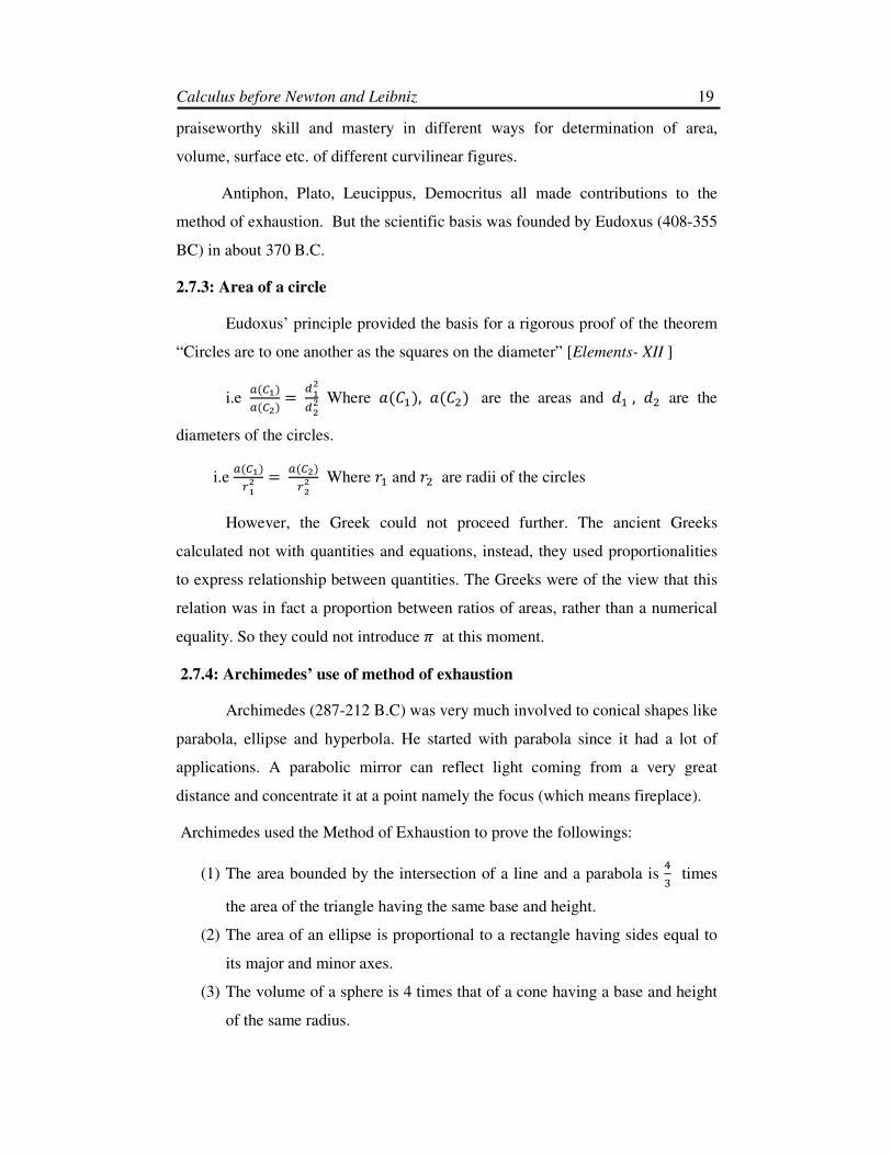
Eudoxus’ principle provided the basis for a rigorous proof of the theorem

“Circles are to one another as the squares on the diameter” [Elements- XII ]

i.e �(��)�(��) � ��

Where �(��), �(��) are the areas and �� , �� are the

diameters of the circles.

i.e �(��)

�� (��)

�� Where �� and �� are radii of the circles

However, the Greek could not proceed further. The ancient Greeks

calculated not with quantities and equations, instead, they used proportionalities

to express relationship between quantities. The Greeks were of the view that this

relation was in fact a proportion between ratios of areas, rather than a numerical

equality. So they could not introduce at this moment.

2.7.4: Archimedes’ use of method of exhaustion

Archimedes (287-212 B.C) was very much involved to conical shapes like

parabola, ellipse and hyperbola. He started with parabola since it had a lot of

applications. A parabolic mirror can reflect light coming from a very great

distance and concentrate it at a point namely the focus (which means fireplace).

Archimedes used the Method of Exhaustion to prove the followings:

(1) The area bounded by the intersection of a line and a parabola is �� times

the area of the triangle having the same base and height.

(2) The area of an ellipse is proportional to a rectangle having sides equal to

its major and minor axes.

(3) The volume of a sphere is 4 times that of a cone having a base and height

of the same radius.


(4) The volume of a cylinder with a height equal to its diameter is �� that of a

sphere having the same diameter.

(5) The area bounded by one spiral rotation and a line is �� that of a circle

having a radius equal to the length of line segment. Archimedes’ works on

area and volume can be arranged in the following order:

(i) Measurement of a circle

(ii) Quadrature of a parabola

(iii) On the sphere and cylinder

(iv) On spirals

(v) On conoids (Paraboloid and Hyperboloid)

(vi) The Method

Method of exhaustion was proved to be a technique of amazing power in

the first five of these above. But Archimedes failed to find areas of elliptical and

hyperbolic sectors. These computations become possible after the development of

integral calculus only.

Archimedes developed the “method of compression” also. By this

method, the area of a circle was compressed between the areas of inscribed and

circumscribed polygons [Fig.2.4], the volume of a paraboloid was compressed

between the volumes of inscribed and circumscribed cylinders [Fig.2.5(a) &(b)].

The method was extensively used by Archimedes (287-212 BC) to derive

arithmetic formulae for areas of other geometric figures also.

Fig.2.4: Exhausting the area of a circle

Calculus before Newton and Leibniz

Fig. 2.5 (a)

Exhausting the area of a solid of

Fig.2.6 : Exhausting the area of a segment of a parabola

Fig.2.7 : Exhausting the area of a spiral rotation and a line segment

2.7.5: Comments

Archimedes’ efforts were dependent on the shape of the curves and solids.

It required a lot of algebraic skills; because of non

algorithms at that time. The absence of sufficient knowledge of algebra made

Archimedes to refrain himself

curves and solids. He used cumbersome ‘double reductio ad absurdum’ method

to find the areas and volumes.


(a) Fig. 2.5 (b)

Exhausting the area of a solid of revolution (paraboloids)

Exhausting the area of a segment of a parabola

Exhausting the area of a spiral rotation and a line segment


It required a lot of algebraic skills; because of non-availability of any kind


himself from finding areas and volumes of many other


mes.

21

Exhausting the area of a spiral rotation and a line segment


availability of any kind of


from finding areas and volumes of many other



2.7.6: Euclid’s use of Method of exhaustion

To the Greeks, the age old concept of finding area of planer regions and

volumes of solids were important. Appearing in Book XII of Euclid’s Elements,

the method was proved to be fundamentally critical in the following centuries.

Euclid used the Method of Exhaustion for finding the relative volumes of cones,

pyramids, cylinders and spheres in the following six propositions of Book XII of

Elements.

(1) The area of a circle is proportional to the square of its diameter (Prop – 2)

(2) The volumes of two tetrahedrons of the same height are proportional to

the areas of their triangular bases. (Prop – 5)

(3) The volume of a cone is a third of the volume of the corresponding

cylinder having the same base and height. (Prop – 10)

(4) The volume of a cone (or cylinder) of the same height is proportional to

the area of the base. (Prop – 11)

(5) The volume of a cone (or cylinder) similar to another is proportional to

the cube of the ratio of the diameters of the bases. (Prop – 12)

(6) The volume of a sphere is proportional to the cube of its diameter.

(Prop – 18)

The concepts of infinity and limit were absorbed in Eudoxus’ principle.

The Greek mathematicians used magnitudes that can be made as large or as small

in place of infinitely large or small.

It only provides a technique for calculating certain continuous

magnitudes and gives rise to approximate calculations.

2.8: QUADRATURE

The problem of quadrature was a problem for the ancient mathematicians

also. The problem exhibits a square of the same area of a given figure. To find a

quadrature of a rectangle of length a and breadth b, one must have a square of

side equal to √�� . To find a quadrature of a triangle, we must have a rectangle of

same area equal to that of a triangle and then a square equal to the area of the

rectangle.


The Greek mathematicians took the chall

‘rectification of a circle’.

dividing it into small rectangular strips of two types. The

(i) first gives the area of the

(ii) the other gives the area of the rectangles circumscribing the

Circle.

Difference between the two areas becomes smaller and smaller when the

number of rectangles is increased or the width of the rec

However, this of course is an early example of integrat

2.8.1:The quadrature of segment of a parabola

The quadrature of a ci

out by the earlier mathematicians. But nobody attempted

segments of a parabola. Archimedes was the first to attempt to find the area of a

segment of a parabola using the me

originality. It was clearly mentioned in the preface of the

parabola.

To find the area of a parabolic segment, Archimedes considered a certain

inscribed triangle, the base of which

vertex is the point of tangency such that the tangent at the third vertex is parallel

to the chord.


The Greek mathematicians took the challenge of ‘squaring of a circl

circle’. Archimedes was able to perform a quadrature by

ngular strips of two types. The

first gives the area of the rectangles inscribed in the circle

the other gives the area of the rectangles circumscribing the

Fig. 2.8

ifference between the two areas becomes smaller and smaller when the

number of rectangles is increased or the width of the rectangles is decreased.

his of course is an early example of integration.

:The quadrature of segment of a parabola

The quadrature of a circle or segment of a circle was successfully found

out by the earlier mathematicians. But nobody attempted to find the area of

of a parabola. Archimedes was the first to attempt to find the area of a

segment of a parabola using the method of exhaustion with high standard of

originality. It was clearly mentioned in the preface of the Quadrature of the


inscribed triangle, the base of which is a given chord of the parabola and the third


Fig. 2.9

23

circle’ and

s able to perform a quadrature by

the other gives the area of the rectangles circumscribing the

ifference between the two areas becomes smaller and smaller when the

tangles is decreased.

successfully found

the area of

of a parabola. Archimedes was the first to attempt to find the area of a

thod of exhaustion with high standard of

Quadrature of the


given chord of the parabola and the third



The following facts related to parabolic segment APB were known during

Archimedes’ time

(i) Tangent line at P is parallel to AB.

(ii) The straight line through P parallel to the axis intersects the base AB at

its midpoint M.

(iii) Every chord parallel to the base AB is bisected by the diameter PM

(iv) With the notation in Fig.2.9, � �! � ��

!"� [26]

Applying these, Archimedes found the area of a parabolic segment

� � ��

�� , , , , , , , , ��# …………. (1)

where a is the area of the triangle APB.

To determine the sum of the series, Archimedes used the following

method-- given a series of areas A,B,C,D, …….,Y, Z such that A is the greatest

and each is equal to 4 times the next i.e

A=4B, B=4C, C=4D, ……….,Y=4Z.

Now, B+C+D+ ……+Y+Z +B/3+C/3+ ……..+Y/3+Z/3…….(1)

= 4B/3+4C/3+4D/3+………….+4Y/3+4Z/3

= (4B+4C+4D+………….+4Y+4Z)/3

= A/3+ (B+C+………………….+Y)/3

On the other hand,

B/3+C/3+…………+Y/3 = (B+C+……….+Y)/3………(2)

(1) –(2) gives

B+C+D+…………..+Y+Z+Z/3 = A/3

gives

A+B+C+D+ …………+ Z+Z/3 = 4A/3

i.e A (1 ��

�$ �$� ⋯ … … … … … …) = 4A/3

1 ��

�$ �$� ⋯ … … … … … =

��

This is the first known example of summation of infinite series.


2.8.2: Visual demonstration of sum of

Sum of areas of white squares =

Sum of areas of black squares

Sum of areas of grey squares =

The area of the biggest square = 3

Hence, 4

1

4

11

2+++

2.8.3: Comments

Here, we have observed that above

(geometric series with common

series permits one to get a finite sum of infinite number of summands.

luckily Archimedes faced

terms to infinity in this series.

development of calculus. The first example of a g

is due to the Babylonians (

of geometric series is found in Ahmes Rhind papyrus (


demonstration of sum of the above series

Fig.2.10: Unit square

Sum of areas of white squares = .........4

1

4

1

4

132

++

Sum of areas of black squares = .........4

1

4

1

4

132

++

Sum of areas of grey squares = .........4

1

4

1

4

132

++

The area of the biggest square = 3× ( .........4

1

4

1

4

132

++ ) = 1

.........4

13

= 3

4

Here, we have observed that above infinite series is a convergent

(geometric series with common ratio 14

1∠ ) whose sum is

4

11

1

−

=� � . Convergent

series permits one to get a finite sum of infinite number of summands.

luckily Archimedes faced no difficulty in extending sum of finite number of

in this series. Geometric series played a crucial role to the

The first example of a geometric series yet discovered

due to the Babylonians (2000 BC). In Egyptian mathematics, the first problem

found in Ahmes Rhind papyrus (1500 BC). It is as follows:

25

infinite series is a convergent series

Convergent

series permits one to get a finite sum of infinite number of summands. Here,

extending sum of finite number of

Geometric series played a crucial role to the

yet discovered

matics, the first problem

1500 BC). It is as follows:


Household------------ 7

Cats ------------- ----- 49

Mice ------------------ 343

Barley (spelt) ------- 2301

Heek measures ----- 16807

Total -------- 19607 [65]

Euclid gave one problem that may be expressed as

1

12

11

11

.......... a

aa

aaa

aa

nn

n −=

+++

−

−

+ which amounts to saying a

aar

s

aar

n

n −=

−.

During medieval times, Bhaskara (1150) gave a problem like this; “A person

gave a mendicant a couple of cowry shells first; and promised a two fold increase

of the alms daily. How many nischas does he give in a month?”

[1 nischas = 16× 6 × 4 × 20 cowry shells]

It is equivalent to finding 3132 2..........222 ++++ .

Walli’s method of finding area under a hyperbola led Newton to deal with

geometric series. The convergence of geometric series reveals that a sum

involving an infinite number of summands can be finite. But Archimedes used

‘reductio ad absurdum’ method to avoid the summation of infinite series. Zeno’s

assumption was that infinite number of finite steps cannot be finite. For this

reason, Zeno’s paradoxes could not be resolved.

2.9: SOLIDS OF REVOLUTION

Archimedes used the method of compression that is most closely to the

construction underlying the modern definite integral in his treatise “On Conoids

and Spheroids”. A conoid is what we would call a paraboloid or hyperboloid of

revolution and a spheroid is an ellipsoid of revolution.

He showed the volume of a paraboloid of revolution P inscribed in a

cylinder C with radius R and height H

v (P) � �� × volume of the circumscribed cylinder

� �� R2

H


To prove this result, he constructed n- slices of equal thickness ℎ � ()

that can be proved by modern integral calculus also.

Archimedes used this slicing construction method for finding the volumes

of segments of ellipsoids and hyperboloids of revolution cut off by planes that are

not necessarily perpendicular to the axes of the figures by employing a common

general modus-operandi-a logical step to the formulation of a general concept of

integration.

Dividing volumes and areas into the sum of a large number of individual

pieces, he basically used the limiting process of integral calculus 2000 years

before Newton (1643- 1727) and Leibniz (1646-1716).

Works of Archimedes hardly survived during the so called Dark Ages

(500AD-1000 A.D). Almost all translations of Archimedes’ work were ultimately

vanished except Latin translation of The Method, without a trace in the 16th

century. But the idea he planted, gave a glimpse to what may be called the

technique of calculus. Many of his solutions can be viewed as computations of

definite integral of the form * (�� ) ��+ .

2.10: FAILURE OF THE GREEKS

The failure of the Greeks in inventing integral calculus can be thought

mainly for two reasons:

(i) their discomfort with the concept of infinity.

(ii) their lack of sufficient knowledge of algebra due to lack of proper

notation and inability to deal with equations.

2.11: ERA OF TRANSLATIONS

During the 7th

and 8th

centuries, the Muslim empire extended towards

Persia, Syria in the east and to Spain, Morocco in the west. There were several

mathematicians and astronomers working at Baghdad during the early 9th

century. Among them Al- Khowarizmi was the most eminent astronomer and

mathematician. He wrote text books on Arithmetic and Algebra viz Al- jabar

wa’l muqabalah.


During the 9th

and 10th

centuries, many books of Archimedes, Apollonius

and Ptolemy including Euclid’s Elements were translated from Greek to Arabic.

Christian scholars visited Spain and Sicily to acquire Moslem learning. During

11th

century, Greek classics were translated from Arabic to Latin by the Christian

scholars of Europe by the opening of Western European commercial relation with

the Arabian world. 12th

century became a century of translations. One of the most

eminent translators of this period was Gherado of Cremona. He translated more

than ninety Arabian books to Latin among which many books of Archimedes

were included. In the meantime, eastern civilization where arithmetic and algebra

were extensively studied came in touch with the Italian merchants. They played

an important role in spreading Hindu -Arabic system of numeration in Europe.

By the 12th century, development of Arabic science began to turn down

with the rise of Western Europe. During this era of translation and propagation;

idea of motion, variability and the infinite together with the symbolic algebra and

analytic geometry were merged. This amalgamation paved the way for invention

and growth of mathematics related to infinitesimals in 17th century.

On the other hand, the Hindus in India were very much interested in

numbers including irrationals and had little interest in geometry and deductive

methods. This is one of the distinguishing features of Greek as well as Indian

mathematics.

2.12: MEDIEVAL THOUGHTS

In the 13th century, universities at Paris, Oxford, Cambridge, Padua and

Naples came into being and became the powerful factors in the development of

mathematics. Campanus’ Latin translation of Euclid’s Elements printed in 1482

became the first printed version of Euclid’s great book. The impact of the era of

translation on newly founded universities brought back quantitative science in

Western Europe. Yet, one would be surprised to know that Archimedes’ works

drew no significant attention from the scholars at that time also.

2.12.1: Concept of changeable things and Merton Scholars

Aristotle’s Treatise on Physics explored the nature of infinite and the

existence of indivisibles or infinitesimals and the divisibility of continuous


quantities- time, motion and geometric magnitudes. Aristotle observed that

motion was itself continuous and infinite was present in it. The definition of

continuity was given as “what is infinitely divisible is continuous” [26].

The problem of changeable things was first successfully studied by a

group of logicians and natural philosophers at Merton College in oxford in 14th

century. During 13th century, Aristotelian thoughts influenced the western

intellectuals. William Heytesbury (before 1313-1372), Richard Kelvington, John

Dumbleton, Thomas Bradwardine (later Archbishop of Canterbury) and Richard

Swineshead were also the Mertonian scholars. They sought to study variations in

the intensity of a quality, intensive or local (such as hotness, density) and

extensive or global (such as heat, weight).

2.12.2: Mean Speed Theorem (MST)

The Merton scholars investigated velocity as a measure of motion.

According to Aristotle, all the qualities of a body (temperature, size and place)

could change. But the central issue relating to the motion as interpreted by the

Merton scholars was the ‘change of place’. They defined uniform motion (or

constant speed) as the equal distances described in equal times and uniform

acceleration as that for which equal increments of velocity acquired in equal

intervals [19]. In spite of this, ‘instantaneous velocity’ was not perfectly defined

due to the lack of notion of ‘limits of ratios’. They could work only in the light of

Euclid i.e with proportions of equivalent units.

William Heytesbury is well known for developing the rule of uniform

acceleration i.e. the Mean Speed Theorem which was stated in 6th

chapter of his

work Regulae Solvendi Sophismata in the following way:

‘If a moving body is uniformly accelerated during a given time interval,

then the total distance S traversed is that which it would move during the same

time interval with a uniform velocity equal to the average of its initial velocity v0

and its final velocity vf (namely, its instantaneous velocity at the mid pt. of the

time interval)’

i.e S � �� ,-. -/0 1 where t is the length of time - interval.


In this way, emergence of kinematics took place at Merton College.

Merton’s studies became popular and

the mid - 14th century. These medieval scholars demonstrated thi

foundation of the “law of falling bodies”

physicist and historian of science Clifford

History of Mechanics wrote

contention, that the main kinematical properties of uniformly accelerated

motions, still attributed to Galileo by the physics texts, were discovered and

proved by scholars of Merton college…….. In principle,

physics were replaced, at least for motions, by the numerical quantities that have

ruled western science ever since.”

2.12.3: Nicole Oresme and

Nicole Oresme, a

Configurations of Qualities and Motions

representations of intensities of qualities connecting geometry and the physical

world which became a “second characteristic

He discussed mainly in

measured by an interval (alien segment) of either space or time.

intensity of quality at each p

segment at that point, thereby constructing a graph with the reference interval as

its base. Reference interval and its intensity at a p

and latitude respectively which we des

This graphical presentation produced

simple but influential step to

Fig. 2.11: Graphical representation of MST


emergence of kinematics took place at Merton College.

studies became popular and was spread to France and Italy in

century. These medieval scholars demonstrated this theorem as the

law of falling bodies” long before Galileo. The mathematical

physicist and historian of science Clifford A.Truesdell in his book Essays in the

wrote,“ The now published sources prove to us, beyond



proved by scholars of Merton college…….. In principle, the qualities of Greek

, at least for motions, by the numerical quantities that have

ruled western science ever since.”

Nicole Oresme and Graphical representation

Persian scholar in 1350 wrote his Treatise on the

gurations of Qualities and Motions and introduced the concept of graphical


world which became a “second characteristic habit” of western thought.

He discussed mainly in case of a ‘linear’ quality whose ‘extension’ was

measured by an interval (alien segment) of either space or time. He measured the

quality at each point of the reference interval by a perpendicular line

thereby constructing a graph with the reference interval as

its base. Reference interval and its intensity at a point were said to be longitude

respectively which we designate as the abscissa and ordinate

presentation produced by Oresme marked his demonstration,

simple but influential step towards the development of calculus.

2.11: Graphical representation of MST

30

emergence of kinematics took place at Merton College.

spread to France and Italy in

s theorem as the

The mathematical

Essays in the

“ The now published sources prove to us, beyond



of Greek

, at least for motions, by the numerical quantities that have

Treatise on the

and introduced the concept of graphical


case of a ‘linear’ quality whose ‘extension’ was

He measured the

ular line

thereby constructing a graph with the reference interval as

longitude

te as the abscissa and ordinate today.

marked his demonstration, a


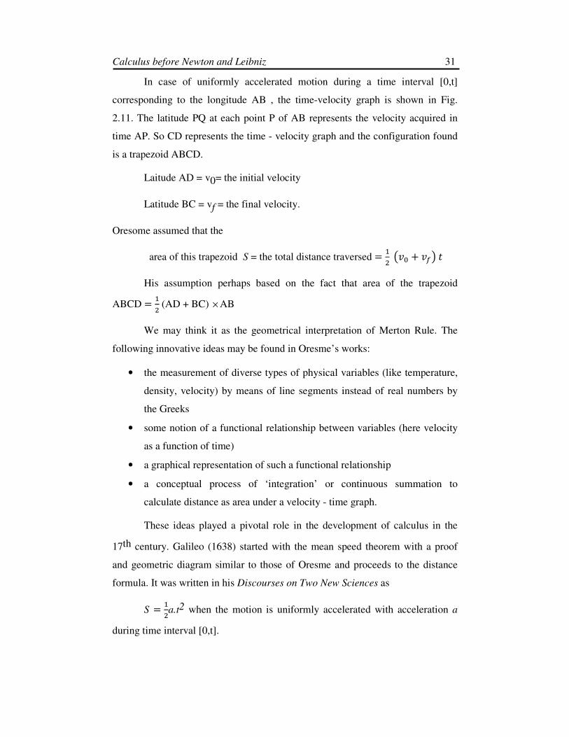
In case of uniformly accelerated motion during a time interval [0,t]

corresponding to the longitude AB , the time-velocity graph is shown in Fig.

2.11. The latitude PQ at each point P of AB represents the velocity acquired in

time AP. So CD represents the time - velocity graph and the configuration found

is a trapezoid ABCD.

Laitude AD = v0= the initial velocity

Latitude BC = vf = the final velocity.

Oresome assumed that the

area of this trapezoid S = the total distance traversed � �� ,-. -/0 1

His assumption perhaps based on the fact that area of the trapezoid

ABCD � �� (AD + BC) × AB

We may think it as the geometrical interpretation of Merton Rule. The

following innovative ideas may be found in Oresme’s works:

• the measurement of diverse types of physical variables (like temperature,

density, velocity) by means of line segments instead of real numbers by

the Greeks

• some notion of a functional relationship between variables (here velocity

as a function of time)

• a graphical representation of such a functional relationship

• a conceptual process of ‘integration’ or continuous summation to

calculate distance as area under a velocity - time graph.

These ideas played a pivotal role in the development of calculus in the

17th century. Galileo (1638) started with the mean speed theorem with a proof

and geometric diagram similar to those of Oresme and proceeds to the distance

formula. It was written in his Discourses on Two New Sciences as

S � ��a.t2 when the motion is uniformly accelerated with acceleration a

during time interval [0,t].


2.12.4: The Infinite and Merton Scholars

One of the Merton scholars, Swineshead

path of Aristotle who lived in 4

“if a point moves throughout the first half of a certain time interval with a

constant velocity , throughout the next quarter of the interval at double the initial

velocity , throughout the following eighth at tripl

ad. infinitum; then the average velocity during the whole time interval will be

double the initial velocity.”

Taking both time interval and initial velocity as unity, he got the

following series from the above pr

++ 34

1.2

2

1

This is the second infinite series appeared in the history of mathematics

after the infinite series

4

1

4

11

2+++

deduced by Archimedes used in the

To find the summation of the series (1), Oresme gave a geometrical proof

in his Treatise on Configuration

The area covered in Fig.2.12

Fig. 2.13(a) Fig


The Infinite and Merton Scholars

One of the Merton scholars, Swineshead studied the infinite following the

path of Aristotle who lived in 4th

century BC. He solved a problem stated as:



out the following eighth at triple the initial velocity , and so on


.” [26]


following series from the above problem

∞+++ .......................2

1.......................

8

1.3

nn ……..


3

4.......................

4

1...................

4

13

=∞++++n

used in the Quadrature of the Parabola.

summation of the series (1), Oresme gave a geometrical proof

Treatise on Configuration which is explained in Fig. 2.12(a) and 2.12

Fig.2.12(a) is same as area covered in Fig 2.12(b).

2.13(a) Fig. 2.13(b)

32

studied the infinite following the

solved a problem stated as:



e the initial velocity , and so on



…….. (1)


summation of the series (1), Oresme gave a geometrical proof

which is explained in Fig. 2.12(a) and 2.12(b).


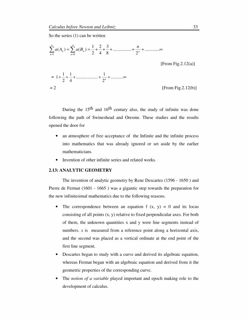
So the series (1) can be written

∞+++++==∑∑∞

=

∞

=

.............2

................8

3

4

2

2

1)()(

01n

n

n

n

n

nBaAa

[From Fig.2.12(a)]

∞+++++ ...........

2

1...................

4

1

2

11

n

= 2 [From Fig.2.12(b)]

During the 15th and 16th century also, the study of infinite was done

following the path of Swineshead and Oresme. These studies and the results

opened the door for

• an atmosphere of free acceptance of the Infinite and the infinite process

into mathematics that was already ignored or set aside by the earlier

mathematicians.

• Invention of other infinite series and related works.

2.13: ANALYTIC GEOMETRY

The invention of analytic geometry by Rene Descartes (1596 - 1650 ) and

Pierre de Fermat (1601 - 1665 ) was a gigantic step towards the preparation for

the new infinitesimal mathematics due to the following reasons.

• The correspondence between an equation f (x, y) = 0 and its locus

consisting of all points (x, y) relative to fixed perpendicular axes. For both

of them, the unknown quantities x and y were line segments instead of

numbers. x is measured from a reference point along a horizontal axis,

and the second was placed as a vertical ordinate at the end point of the

first line segment.

• Descartes began to study with a curve and derived its algebraic equation,

whereas Fermat began with an algebraic equation and derived from it the

geometric properties of the corresponding curve.

• The notion of a variable played important and epoch making role to the

development of calculus.

=


And thus analytic geometry opened up a vast field for the use of

infinitesimal technique by using variety of curves.

2.14: CAVALIERI AND KEPLER

The systematic study and use of infinitesimal techniques for area and

volume computations was popularized by two outstanding books written by

Bonaventura Cavalieri (1598 -1647), a countryman and pupil of Galileo (1564 -

1642). These books were Geometria Indivisibilibus continuorum (Geometry of

indivisibles) and Exercitationes Geometricae Sex (six geometrical exercises) of

1647. Brief English translations of these books may be found in Struik’s source

book [71]. These publications exerted enormous influence upon the development

of infinitesimsl calculus of later period. Johan Kepler (1571 - 1630) studied area

and volume problems needed for his astronomical studies.

Cavalieri’s method differs from that of Kepler in the following aspects:

• Kepler considered a given geometrical figure to be decomposed into

infinitesimal figures and summing up the areas and volumes of these

infinitesimal figures obtained the area and volume of the whole figure.

Kepler in his work on planetary motion had to find the area of sectors of

an ellipse.

• Kepler’s consideration of infinitesimal figures are of the same dimension

as that of the geometrical figure. To find area (volume) of a figure, he

needed area (volume) of indivisibles.

Cavalieri’s method of indivisibles consists of two approaches viz.

collective and distributive.

• In collective approach, Cavalieri found by considering a one - to one

correspondence between the indivisible elements of two given

geometrical figures. If ∑ 1l and ∑ 2l be the sums of the line (surface)

indivisibles for two figures 1P and

2P and if β

α=

∑∑

2

1

l

l then

β

α=

2

1

P

P.

Knowing the area or volume of one figure, the area or volume of the

other will be found out.


• In distributive approach,

lower dimension than that of the geometrical figure.

(volume) of two enclosed figures

indivisibles parallel and equidistant

respectively. For corresponding line segments (

if 1l = 2l then 1C =C

Cavalieri’s method showed greater generality and a more abstractness in

the method of treatment than that of Kepler.

For example, to derive the volume of a circular cone

and height is h, Cavalieri proceeded by comparing with Pyramid

square base and height h. If

section of P with side y at equal distances, then

Important fact to be noticed in Cavalieri’s method is that the indivisible

units may have thickness or not.


In distributive approach, Cavalieri’s consideration of indivisibles are

lower dimension than that of the geometrical figure. To find the area

of two enclosed figures 1C and 2C , Cavalieri considered

indivisibles parallel and equidistant line segments (plane sections

corresponding line segments (plane sections) 1l

2C [Fig-2.13].


the method of treatment than that of Kepler.

Fig. 2.13

For example, to derive the volume of a circular cone C whose base is r

Cavalieri proceeded by comparing with Pyramid P with

. If Cx be the section of C with radius r ′ and Px

at equal distances, then


units may have thickness or not.

35

nsideration of indivisibles are of

To find the area

Cavalieri considered

plane sections)

and 2l ,


ose base is r

with unit

x be the



2.14.1: Comments

In Cavalieri’s method , a geometrical figure is considered to be composed

of infinitely large number of indivisibles of lower dimension such as

(i) area as composed of parallel and equidistant line segments

(ii) volume as composed of parallel and equidistant plane sections.

These important features differ from that of Kepler.

2.14.2: Cavalieri’s new method

Cavaliere devised a new method of calculating the volume of a single

solid in terms of its cross - sections.

Fig. 2.14

For example, let us consider a triangle ABC with base AB and height BC

= a and a typical vertical section PQ of height x .

According to Cavaliere’s sense of indivisibles

Area of ∆ABC = ∑ �"4

We consider a pyramid P whose vertex is A and base is the square drawn

on BC.

The volume of the pyramid 5 � -(5) � ∑ ��"4 thinking of the pyramid as

the sum of its cross - sections.

Also the area under the parabola � � �� is ∑ ��"4


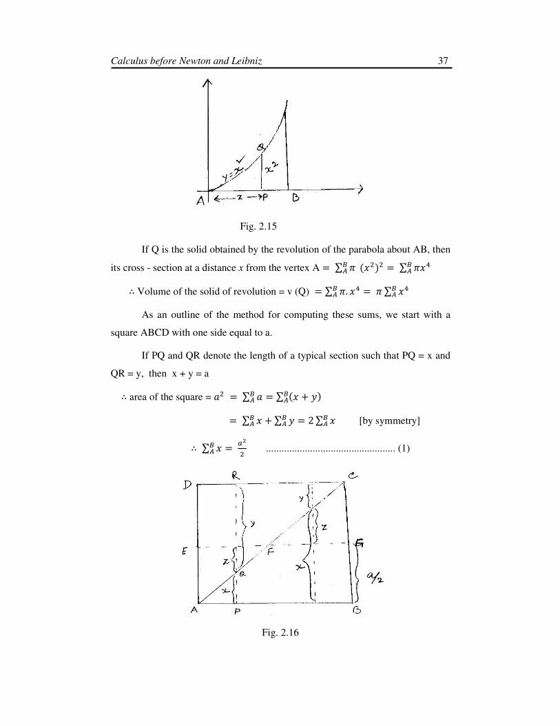
Fig. 2.15

If Q is the solid obtained by the revolution of the parabola about AB, then

its cross - section at a distance x from the vertex A � ∑ "4 (��)� � ∑ ��"4

∴ Volume of the solid of revolution = v (Q) � ∑ . �� ∑ ��"4"4

As an outline of the method for computing these sums, we start with a

square ABCD with one side equal to a.

If PQ and QR denote the length of a typical section such that PQ = x and

QR = y, then x + y = a

∴ area of the square = �� ∑ �"4 � ∑ (� �)"4

� ∑ �"4 ∑ �"4 � 2 ∑ �"4 [by symmetry]

∴ ∑ � � ��"4 .................................................. (1)

Fig. 2.16


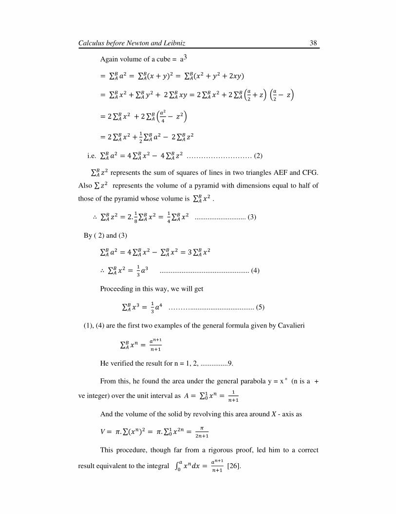
Again volume of a cube = a3

� ∑ ��"4 � ∑ (� �)�"4 � ∑ (�� 2��)"4

� ∑ ��"4 ∑ ��"4 2 ∑ ��"4 � 2 ∑ ��"4 2 ∑ 8�� 9: 8�

� − 9:"4

� 2 ∑ ��"4 2 ∑ 8�� − 9�:"4

� 2 ∑ ��"4 �� ∑ ��"4 − 2 ∑ 9�"4

i.e. ∑ ��"4 � 4 ∑ ��"4 − 4 ∑ 9�"4 ……………………… (2)

∑ 9�"4 represents the sum of squares of lines in two triangles AEF and CFG.

Also ∑ 9� represents the volume of a pyramid with dimensions equal to half of

those of the pyramid whose volume is ∑ ��"4 .

∴ ∑ 9�"4 � 2. �= ∑ ��"4 � �

� ∑ ��"4 ............................ (3)

By ( 2) and (3)

∑ ��"4 � 4 ∑ ��"4 − ∑ ��"4 � 3 ∑ ��"4

∴ ∑ ��"4 � �� ................................................. (4)

Proceeding in this way, we will get

∑ ��"4 � �� ………................................... (5)

(1), (4) are the first two examples of the general formula given by Cavalieri

∑ �) � �#>�)?�"4

He verified the result for n = 1, 2, ...............9.

From this, he found the area under the general parabola y = xn

(n is a +

ve integer) over the unit interval as A � ∑ �)�. � �)?�

And the volume of the solid by revolving this area around X - axis as

V � . ∑(�))� � . ∑ ��) � @�)?��.

This procedure, though far from a rigorous proof, led him to a correct

result equivalent to the integral * �)�� #>�)?�

�. [26].


This is a big leap towards the development of algorithmic procedures of

calculus.

Archimedes proved that the area of the region S bounded by turn of a

spiral and the line segment joining its initial and final points is one third of that of

the circle C centered at the initial point and passing through the final point

i.e. a(S) � �� . . (2 �)�

To prove this he made use of the formulae

1 + 2 + 3 + ...................... + n � )�� )

� -------------------- (1)

12 + 22 + 32 + ................... + n2 � )A� )�

� )$ ----------- (2)

These two formulae play the key role to prove the limits

Lim �?�? …………..? )

)� � ��

B → ∞

B EFGHIJ ∞ ��? ��? ………………..? )�

)A � ��

that was later used to prove the quadrature results

* ��

. and * �� A�

�.

Arabian mathematical science reached its peak in the 11th century. Al-

Haitham (ca. 965-1039) known as Alhazen in the west extended some of

Archimedes’ work on volume results. He showed that if a segment of a parabola

is revolved about its base (rather than about its axis as in Archimedes’ On

Conoids ) then the volume of the solid obtained is 15

8 of that of the circumscribed

cylinder. For this computation, the formulas for the sums of the first n- cubes and

fourth powers are necessary.

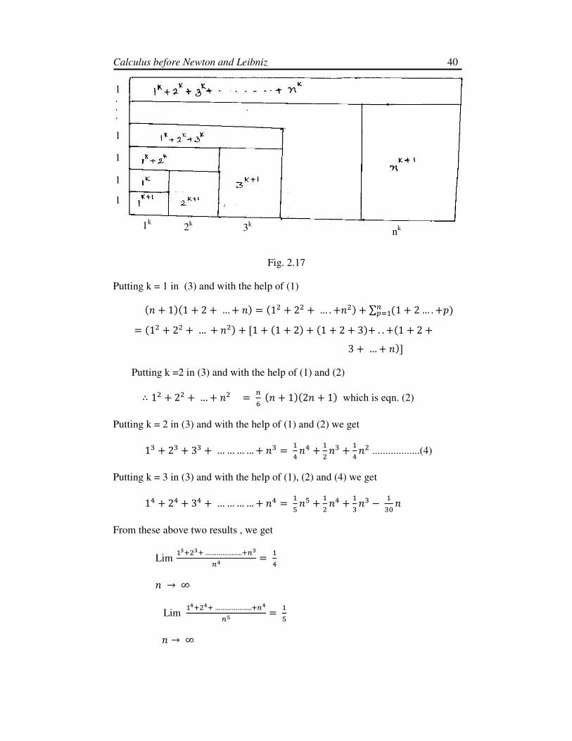
Alhazen proved the formula

(B 1) ∑ KL � ∑ KL?� ∑ ,∑ KLMFN� 0)MN�)FN�)FN� ................. (3)

With the help of a geometric derivation shown in the following figure


Fig. 2.17

Putting k = 1 in (3) and with the help of (1)

(B 1)(1 2 … B) � (1� 2� … . B�) ∑ (1 2 … . O))MN�

� (1� 2� … B�) P1 (1 2) (1 2 3) . . (1 2 3 … B)Q Putting k =2 in (3) and with the help of (1) and (2)

∴ 1� 2� … B� � )$ (B 1)(2B 1) which is eqn. (2)

Putting k = 2 in (3) and with the help of (1) and (2) we get

1� 2� 3� … … … … B� � �� B� �

� B� �� B� ..................(4)

Putting k = 3 in (3) and with the help of (1), (2) and (4) we get

1� 2� 3� … … … … B� � �R BR �

� B� �� B� − �

�. B

From these above two results , we get

Lim �A?�A? ………………..?)A

)S � ��

B → ∞

Lim �S?�S? ………………..?)S

)T � �R

B → ∞

nk 1

k 2

k 3

k

1 . . . 1

1

1

1


In general we can write

Lim 1

1..................211 +

=+++

+ kn

nk

kkk

……………….(5)

B → ∞

Three French mathematicians Fermat, Pascal and Roberval gave more or

less rigorous proofs of the formula * �L�� U>�L?�

�. which was known as

Cavalieri’s (conjectured) general formula for the area under the general parabola

y = xk (k being a +ve integer) i.e. quadrature of the generalized parabola y = xk .

In proving this, each of them used the concept of limit in (5). It required

arithmetical computations only. By simpler arithmetical computations,

Cavalieri’s intuitive ideas of geometrical indivisibles were replaced.

For computation of the area under the curve y = xk over [0, a], the

interval [0, a] is subdivided into n- equal subintervals of length a /n.

Constructing inscribed polygons Pn and circumscribed polygons Qn with

base a/n and height 8�):L , 8��

) :L , 8��) :L , … … … … 8()V�)�

) :L and

8�):L , 8��

) :L , 8��) :L , … … … … 8)�

) :L respectively and making use of the concept

of limit, Fermat, Pascal and Roberval proved that S � �U>�L?� which coincides

with the result * �L�� U>�L?�

�. .

2.15: PROBLEM OF RECTIFICATION

Rectification of an arc of a curve is the construction of a straight line

segment that has equal length of the arc. “Rectification, in geometry, is the

finding of a right line equal to a curve” [18]

Fig. 2.18


It was thought that rectification of an algebraic curve could not be

possible as one would not be able to find the same length of a curve a

constructible straight segment.

A plane curve can be approximated by joining a finite number of points

on the curve using straight line segment to make a polygonal path. Calculating

each linear segment with the help of Pythagoras Theorem one can approximate

the length of the curve.

But it is not always possible for all curves.

Archimedes’ pioneering attempts to find the area beneath a curve by

Method of Exhaustion broke the ground and explored that the approximation of

the length of a curve could be done. In the 17th

century, Method of Exhaustion led

to rectification of curves by geometrical methods of several transcendental

curves, the logarithmic spirals by Evangelista Toricelli in 1645 (some sources say

John Wallis(1616-1703) in 1650 ), the cycloid by Christopher Warren in 1658

and the catenary by Leibniz in 1691. Neil’s rectification of semi-cubical parabola

32 xy = was published in July or August, 1657. It was the first algebraic curve to

be rectified. Wallis published the Method in 1659 giving credit to Neil for his

invention [53].

In 1687, Leibniz raised a question whether the semi-cubical parabola is a

curve along which a particle under gravity may descend so that it traverses equal

vertical distance in equal times? Huygenes proved that it is true for semi-cubical

parabola. So the curve is known as isochronous curve.

2.15.1: Neil’s rectification of algebraic curve

It was commonly believed that an algebraic curve could never have the

same length as a constructible straight line segment. William Neil in 1657 found

the rectification of the algebraic curve known as semi cubical parabola whose

equation given by �� when he was nineteen. His procedure was as

follows:

Let the curve be defined on the interval [0, a]. Subdivide [0, a] into an

indefinitely large number of infinitesimal subintervals. The i-th subinterval is

[ xi-1, yi ]. If si denotes the length (almost straight) of the curve joining


( xi-1 , xi) and ( xi , yi ), then


), then

Fig. 2.19

43


which is equal to the area of the segment of the parabola � � �� 8� �

W:�� lying

over the interval [0, a]. By translating the area will be same as that of the segment

of the parabola 2

1

2

3xy = over [

9

4,

9

4+a ]

Hence, X � �� Y�

� 8� �W:A� − �

� 8�W:A�Z � (W�?�)A�V =

�[

2.15.2: Comments

In Neil’s rectification of a curve y = f (x) over [ 0, a ], we need an

auxiliary curve z = g(x) for which the area Ai over [ 0, xi ] in modern notation is

\F � * ](�)�� ^(�F) � �F_F.

This gives

�F − �FV� � \F − \FV� ≅ ](�F)(�F − �FV�)

So, X ≅ ∑ a1 ,](�)0�b . (�F − �FN�))FN�

� * c1 P](�)Q��. ��

Choosing ](�) � ^d(�) , we get proper auxiliary curve and

X � * e1 P^(�)Qf ��. ��

This is probably the first instance of the interplay between differential and

integral calculus or tangent and quadrature problem.

2.16: TANGENT PROBLEM

2.16.1 Importance of tangent problem

Finding a tangent to a curve was a leading mathematical question of the

early seventeenth century. Because, in optics, the tangent determines the angle at

which a ray of light entered a lens. In mechanics, the tangent determines the

direction of the motion of a body at every point along its path. In geometry, the

tangents to two curves at a point of intersection determines the angle at which

the curves intersected.


Historically, the calculation of areas dates back to many civilizations like

Egyptian, Babylonian, Greek etc. But the problem of finding tangent line to a

curve has long been studied by the Greeks.

2.16.2 Tangent to a circle (Greek view)

The Greeks in Particular, constructed tangent line to a circle at a point on

the circumference. They did it by drawing a radius to a point P on the

circumference and then drawing a line perpendicular to the radius. A tangent line

to a circle at a point indicates the direction of the circle at that point. Important

property of the tangent line to a circle is that it touches the circle, but does not cut

through it. With this property it is not easy to draw a tangent line to most curves.

2.16.3: Tangent to other curves

Apollonius proved many theorems relating to tangent lines to conic

sections. Archimedes determined the tangent line to the spiral. The method of

Archimedes was applied to other curves like cycloid, cissoid etc. by Gilles de

Roberval and Evangelista Torricelli, a student of Galileo in between 1630 and

1640.

Tangent construction to different curves was a major problem to the 17th

century mathematicians. Before Newton and Leibniz, many brilliant

mathematicians like Pierre de Fermat, Rene Descartes. Sluse, Huddes etc. worked

on it. They came upon a different approach to the problem.

2.16.4: Tangent construction by kinematic method

In between 1630 and 1640, Galileo, Evangelista Torricelli (1608 - 1647),

Gilles Personne de Roberval (1602 - 1675), introduced an approach to construct

tangent lines from the intuitive concept of instantaneous motion of a moving

point on a curve. For Archimedean spiral, the motion of the point along the spiral

was considered as the resultant of radial motion (away from the origin) and an

angular motion. For the cycloid, the motion of the point along the cycloid was

considered as the resultant of uniform translation with constant speed and clock-

wise rotation with unit angular speed. Roberval was successful in obtaining the

tangent lines to the parabola and ellipse by this method.


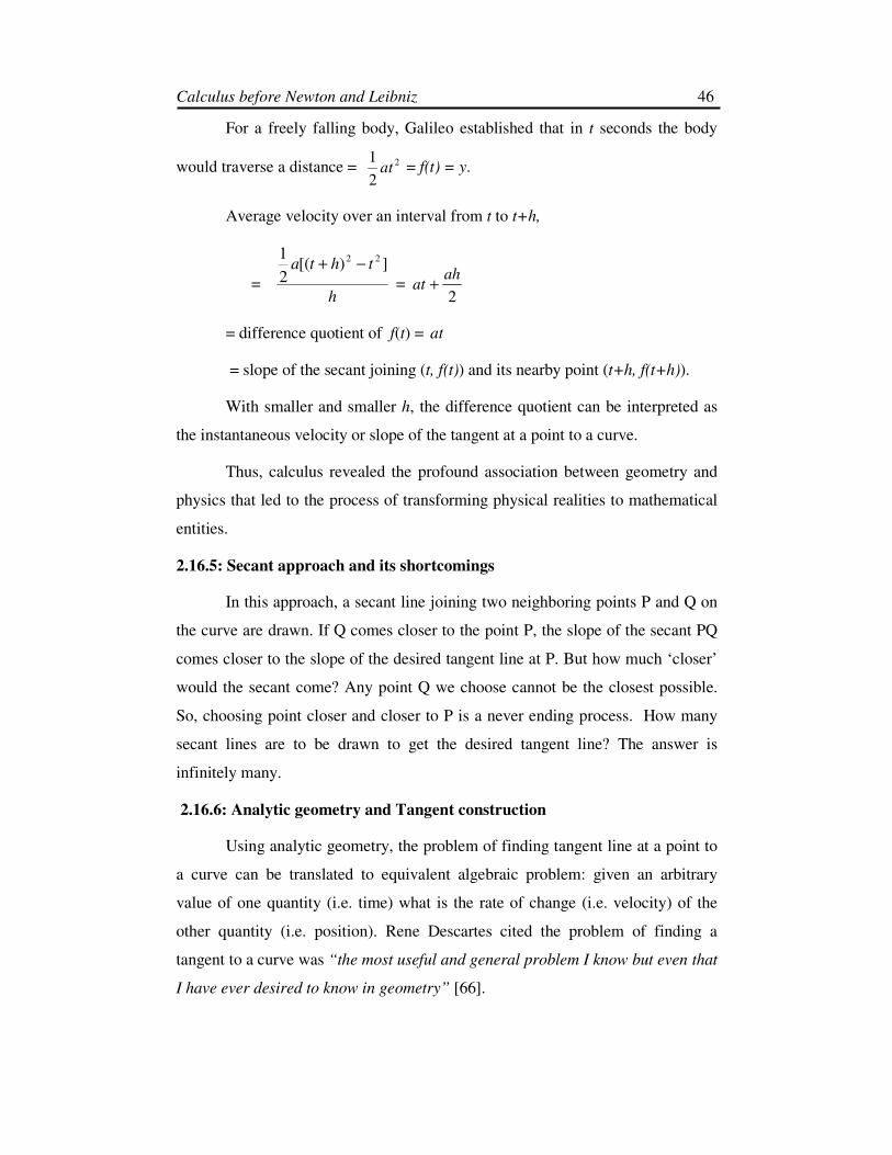
For a freely falling body, Galileo established that in t seconds the body

would traverse a distance = 2

2

1at = f(t) = y.

Average velocity over an interval from t to t+h,

= h

thta ])[(2

1 22 −+ =

2

ahat +

= difference quotient of f(t) = at

= slope of the secant joining (t, f(t)) and its nearby point (t+h, f(t+h)).

With smaller and smaller h, the difference quotient can be interpreted as

the instantaneous velocity or slope of the tangent at a point to a curve.

Thus, calculus revealed the profound association between geometry and

physics that led to the process of transforming physical realities to mathematical

entities.

2.16.5: Secant approach and its shortcomings

In this approach, a secant line joining two neighboring points P and Q on

the curve are drawn. If Q comes closer to the point P, the slope of the secant PQ

comes closer to the slope of the desired tangent line at P. But how much ‘closer’

would the secant come? Any point Q we choose cannot be the closest possible.

So, choosing point closer and closer to P is a never ending process. How many

secant lines are to be drawn to get the desired tangent line? The answer is

infinitely many.

2.16.6: Analytic geometry and Tangent construction

Using analytic geometry, the problem of finding tangent line at a point to

a curve can be translated to equivalent algebraic problem: given an arbitrary

value of one quantity (i.e. time) what is the rate of change (i.e. velocity) of the

other quantity (i.e. position). Rene Descartes cited the problem of finding a

tangent to a curve was “the most useful and general problem I know but even that

I have ever desired to know in geometry” [66].


Systematic methods for the rate of change (i.e. derivative) were developed

by Newton and Leibniz independently with the use of analytic geometry to more

curves [Ch-3] .

2.16.7: Principle of Elimination

The principle of elimination states that “when you have eliminated the

impossible, whatever remains, however improbable, must be the truth” [56].

Sherlock Holmes (1858-1930) used the principle of elimination fruitfully

in his detective novels. Applying this principle in respect of tangent construction

by secant method, when all non - tangent lines to a curve have been eliminated,

the line left would be the tangent line to the curve. For instance, we examine one

problem to understand the principle of elimination and its drawbacks.

Let us consider the simplest form of quadratic function y � �� .

We want to find the slope of the tangent to the curve at P (3, 3 2 ) by the

principle of elimination.

Let Q (3+h, (3+h)2) be another point on the curve near to P (3, 3 2 ) if

ℎ ≠ 0 .

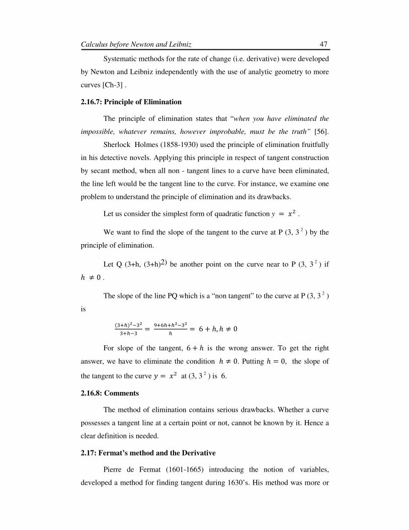
The slope of the line PQ which is a “non tangent” to the curve at P (3, 3 2 )

is

(�?i)�V��

�?iV� � W?$i?i�V��i � 6 ℎ, ℎ ≠ 0

For slope of the tangent, 6 ℎ is the wrong answer. To get the right

answer, we have to eliminate the condition ℎ ≠ 0. Putting ℎ � 0, the slope of

the tangent to the curve � � �� at (3, 3 2 ) is 6.

2.16.8: Comments

The method of elimination contains serious drawbacks. Whether a curve

possesses a tangent line at a certain point or not, cannot be known by it. Hence a

clear definition is needed.

2.17: Fermat’s method and the Derivative

Pierre de Fermat (1601-1665) introducing the notion of variables,

developed a method for finding tangent during 1630’s. His method was more or


less exactly the method used by Newton and Leibniz. He used the notion of limit

in a crude style to invent a workable definition of the slope of a tangent line to a

curve after slight modification of the method of elimination thereby removing the

drawbacks of it.

He first found the slope of the line joining the points P (c,f (c)) and Q

(c+h, f (c+h)) where ℎ ≠ 0 The slope of PQ is /(+?i)V/(+)

i which is not our

desired slope of the tangent line. So to define the slope of the tangent at (c, f (c))

to be the number (if there is one) that the above expression tends to that number

as h approaches zero. Fermat’s idea is easy. The right answer is the limiting

value of the wrong answer.

He discovered the formula for finding tangent to the curve � � �), the

slope of such a tangent line is B�). For this and other results, Fermat is considered by Lagrange and many, to

be the inventor of differential calculus, although his work did not approach the

generality of Newton or Leibniz [66].

2.17.1: Fermat’s pseudo-equality∗∗∗∗ (adequality) method

The problem of construction of tangent lines to general curves was not

studied until the middle decades of the 17th century. It was one of the major

problems facing the mathematicians of 17th century. The tangent or slope of a

curve is so important because it tells us the rate at which something changes. The

rate at which things change, is fundamental in science. Ultimately this problem

was solved by Newton and Leibniz at the end of the century.

In 1635, a few methods for the construction of tangent lines to general

curves were discovered. These methods combined with the area problems and

techniques produced calculus as a new unified method of mathematical analysis.

Fermat’s pseudo- equality method first dealt the solution of maximum- minimum

of a function near an extreme value. His method was formulated in the late

1620’s and published in 1637.

∗ Pseudo-equality- The term pseudo-equality (adequality) was introduced by Fermat to mean an

approximate equality. Fermat said that he had borrowed it from Diophantus.


2.17.2. Fermat’s maxima (

The first problem of maxima or minima dealt by

length b into two segments

Let f(x) = x(b-

For this purpose,

equality’ to compare the resulti

f(x+E ≈ f(x). Because, from intuition or pictorial ground,

slowly when it attains maximum or minimum.

Dividing throughout the result by

i.e setting E = 0 , he obtaine

2.17.3:.Fermat’s tangent construction

To find tangent line to a curve

method. His idea was to find subtangent for the point that

segment on the x-axis between the foot of the ordinate drawn to the point of

contact and the intersection of the tangent line with the x

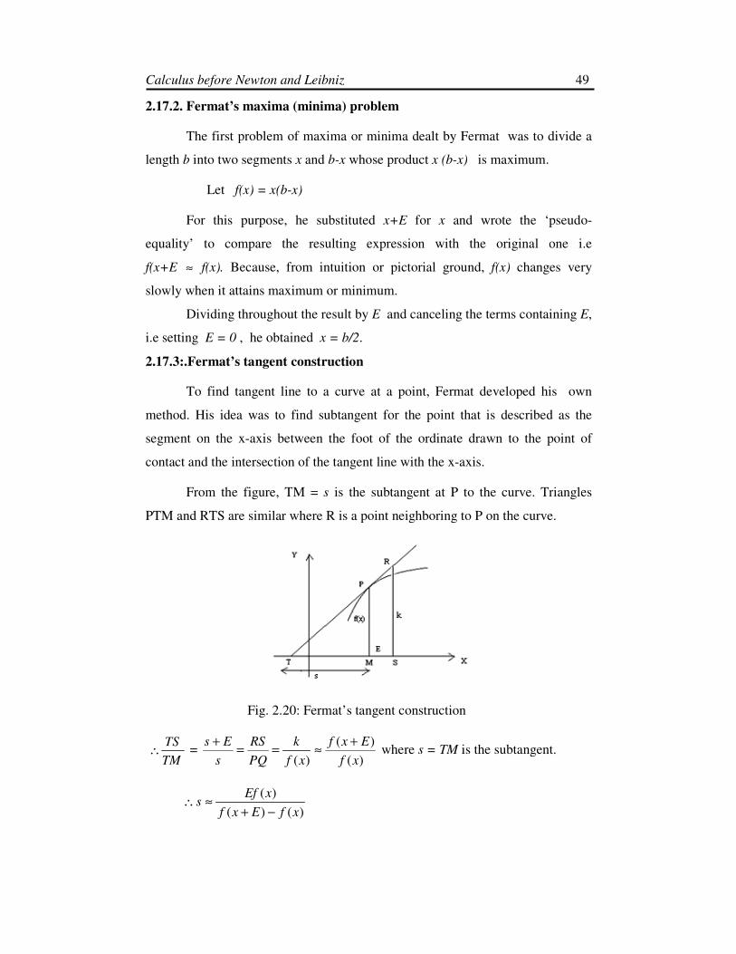
From the figure, T

PTM and RTS are similar where R is a point neighboring to P

Fig. 2.20

TM

TS∴ =

fPQ

RS

s

Es==

+

()(

)(

fExf

xEfs

−+≈∴


Fermat’s maxima (minima) problem

The first problem of maxima or minima dealt by Fermat was to divide a

into two segments x and b-x whose product x (b-x) is maximum.

-x)

he substituted x+E for x and wrote the ‘pseudo

to compare the resulting expression with the original one

Because, from intuition or pictorial ground, f(x) changes very

slowly when it attains maximum or minimum.

Dividing throughout the result by E and canceling the terms containing

ined x = b/2.

Fermat’s tangent construction

To find tangent line to a curve at a point, Fermat developed his

His idea was to find subtangent for the point that is described as the

etween the foot of the ordinate drawn to the point of

contact and the intersection of the tangent line with the x-axis.

TM = s is the subtangent at P to the curve. Tr

where R is a point neighboring to P on the curve.

2.20: Fermat’s tangent construction

)(

)(

)( xf

Exf

xf

k +≈ where s = TM is the subtangent.

)(x

49

o divide a

nd wrote the ‘pseudo-

one i.e

changes very

and canceling the terms containing E,

developed his own

is described as the

etween the foot of the ordinate drawn to the point of

axis.

riangles

on the curve.

is the subtangent.


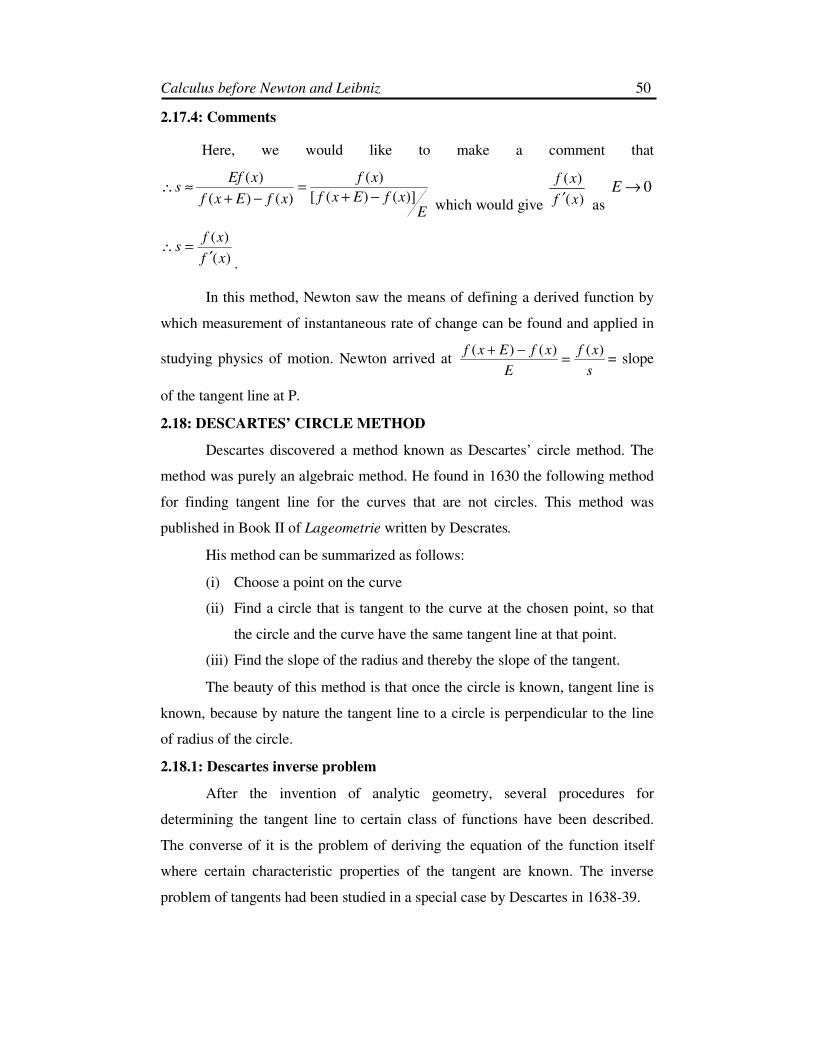
2.17.4: Comments

Here, we would like to make a comment that

ExfExf

xf

xfExf

xEfs

)]()([

)(

)()(

)(

−+=

−+≈∴

which would give )(

)(

xf

xf

′ as

0→E

)(

)(

xf

xfs

′=∴

.

In this method, Newton saw the means of defining a derived function by

which measurement of instantaneous rate of change can be found and applied in

studying physics of motion. Newton arrived at s

xf

E

xfExf )()()(=

−+= slope

of the tangent line at P.

2.18: DESCARTES’ CIRCLE METHOD

Descartes discovered a method known as Descartes’ circle method. The

method was purely an algebraic method. He found in 1630 the following method

for finding tangent line for the curves that are not circles. This method was

published in Book II of Lageometrie written by Descrates.

His method can be summarized as follows:

(i) Choose a point on the curve

(ii) Find a circle that is tangent to the curve at the chosen point, so that

the circle and the curve have the same tangent line at that point.

(iii) Find the slope of the radius and thereby the slope of the tangent.

The beauty of this method is that once the circle is known, tangent line is

known, because by nature the tangent line to a circle is perpendicular to the line

of radius of the circle.

2.18.1: Descartes inverse problem

After the invention of analytic geometry, several procedures for

determining the tangent line to certain class of functions have been described.

The converse of it is the problem of deriving the equation of the function itself

where certain characteristic properties of the tangent are known. The inverse

problem of tangents had been studied in a special case by Descartes in 1638-39.


2.19: HUDDE’S RULE

Hudde discovered a simpler method known as Hudde’s rule. Basically it

involves the derivatives. Descartes’ method and Hudde’s rule were important

because they influenced Newton.

For a given polynomial ∑=

=n

i

i

i xaxF0

)( , consider another polynomial

)(* xF where )(* xF is constructed by arranging the terms of F(x) in order of

increasing degree and multiplied by the terms of an arithmetic progression a,

a+b, a+2b, ………., a+nb

Then, )(* xF = a F(x) + b x )(xF ′ where )(xF ′ = ∑−1i

i xia , the well known

derivative of a polygon.

Hudde’s rule states that any double root of F(x) = 0 must be a root of

)(* xF = 0 i.e any double root of the polynomial F(x) must be a root of its

derivative )(xF ′ .

In particular, Hudde’s rule can be applied to extremum problems also.

The combination of Hudde’s rule and Descartes’ circle method applied only to

algebraic curves written in explicit form y = f (x).

But the Sluse’s method is applicable even to those algebraic curves that

can be written in implicit form ^(�, �) � 0 where ^(�, �) � ∑ k ij � i �F is a

Polynomical in x and y.

Previously, Leibniz accepted Sluse’s rule of tangent without proof. In

November 1676 manuscript, he showed that Sluse’s rule of tangent can be

derived from his calculus also.

2.20: INFINITESIMAL METHOD (BARROW’S METHOD)

The infinitesimal tangent method came into light just after the invention

of algebraic rules of Hudde and Sluse.

Sir Isaac Barrow (1630 -1677), the first Lucassian professor at Cambridge

and the teacher of Sir Isaac Newton, published Optical and Geometrical Lectures

in 1669. In his Geometrical Lectures, he discussed the tangent and quadrature

problem from a classical and geometrical point of view. He used the Greek’s

view of tangent line as a straight line touching the curve at a single point.


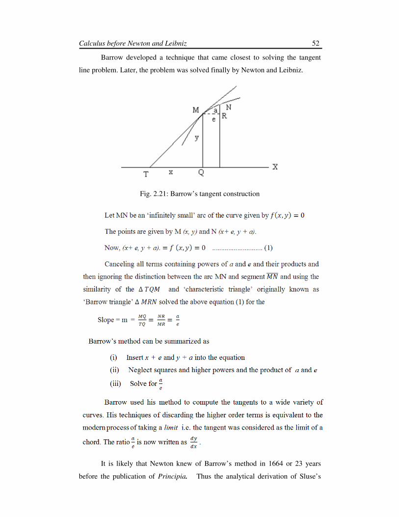
Barrow developed a technique that

line problem. Later, the problem was solved finally by Newton and Leibniz.

Fig. 2.2

It is likely that Newton knew of Barrow’s method in 1664 or 23 years

before the publication of


row developed a technique that came closest to solving the tangent

the problem was solved finally by Newton and Leibniz.

2.21: Barrow’s tangent construction


before the publication of Principia. Thus the analytical derivation of Sluse’s

52

olving the tangent

the problem was solved finally by Newton and Leibniz.


n of Sluse’s


rule was the spirit of Barrow’s approach. Barrow used the concept of

‘characteristic triangle’ which coincides the idea that � → 0, l → 0 (neglecting the ‘higher order differentials’) and the tangent becomes the limiting

position of the secant line.

2.21: A COMPARATIVE DISCUSSION OF DESCARTES, FERMAT AND

BARROW’S METHODS

Before 1665, a few mathematicians could perform tangent construction to

a curve at a point. Descartes, Fermat and Issac Barrow were among them.

Descartes’ method of constructing tangent lines to curves was algebraic

rather than infinitesimal one in character. For this, knowledge of theory of

equations is necessary and it leads to tedious algebraic computations even for a

simple curve. If we compare both the methods of Fermat and Descartes, we find

that the first is much closer to that we are using today. Though, Descartes

technique was not popular due to the complexity involved in it, as much more

precise and fully stuck to geometric techniques; yet the method is considered

mathematically sound method of computation of tangent line.

Fermat’s method of finding tangents seems to have been a bi-product of

his method of finding maxima and minima. His idea was set forth in 1629 in a

letter written to a certain M. Despagnet. Fermat was of the view that finding the

tangent did not mean finding its equation, but finding the sub-tangent.

In Fermat’s method, the point R neighboring to P lies on the tangent line

drawn at P on the curve [Fig.2.20]. Fermat used sub-tangent, abscissa, and

ordinates of the points P and R to find sub-tangent. He introduced a ‘small’ or

‘infinitesimal’ element E to the abscissa. Fermat gave several examples of the

application of his method. Some of his results were published by Pierre Herigone

in his Supplementum Curses mathematici (1642). He could find tangents to all

curves given by polynomial equations y = p(x) and probably to all algebraic

curves.

Issac Barrow, in his book Lectiones Opticae el geometricae written

apparently in 1663, 1664 and published in 1669, 1670, gave his method of

tangents. Before him, Roberval and Torricelli found tangent lines to a curve

compounding two velocities in the direction of the axes of x and y to get a

resultant along the tangent line.


In Barrow’s method, the point N neighboring to P lies on the curve itself

[Fig.2.21]. The increments MR and NR of the abscissa and ordinate were denoted

by e and a and the ratio a:e was determined by substituting x+e for x and y+a for

y in the equation of the curve, rejecting all terms of order higher than the first in

a and e. He introduced two infinitesimal quantities a and e. Their ratio is

equivalent to Leibniz’ symbol dx

dy. This process is equivalent to differentiation.

∆ MNR is sometimes called Barrow’s differential triangle.

Barrow went further than Fermat in the theory of differentiation as he

compared two increments. But Fermat’s trick may be noted as the fundamental

trick in infinitesimal calculus. The formal algorithms for the construction of

tangents were invented by the Dutch mathematicians Hudde and Rene Francois

de Sluse in 1650.

2.22: AREA AS ANTIDERIVATIVE

Fig. 2.22: Equality of the area of the circle and the triangle

In the above figure, we may have three cases

(i) the area A of the circle is greater than the area of the triangle

(ii) the area A of the circle is smaller than the area of the triangle

(iii) the area A of the circle is equal to the area of the triangle

Archimedes proved (iii) by ‘reductio ad absurdum’ method as (i) and (ii)

give rise to contradictions.

Then \ � �� . � , where C is the circumference and r is the radius

of the circle.

⇒ � � 2 �


� � 2 � represents a straight line of slope 2 passing through the

origin. The variables A, C, r are indicated as in the figure below:

For a change ∆� of r, ∆k of C,

Fig. 2.23

rCrCA ∆∆+∆=∆ ).(2

1.

∴ ∆4∆� � � �

� (∆�)

As ∆� → 0, ∆k → 0 �B� ∆� → 0, ∆4∆� → �

i.e. the area beneath a curve (a continuous function) is related to the function i.e.

area be an antiderivative of y where y is a function of x.

Leibniz guessed it in about 1670 and Newton guessed it in 1666, but he

kept it secret.

2.23: INTERPLAY BETWEEN AREA AND TANGENT

Torricelli and Issac Barrow were the first to make an association between

tangent and area problems with the help of time and motion concepts. Both of

them considered the problem of the motion of a point along a straight line with

varying velocity. It can be represented pictorially by a velocity-time graph. It was

first suggested by Galileo. The total distance covered by the point will be equal to

the area under the velocity - time graph.

For the velocity –time graph of - � 1) in the interval P0, 1Q, then by the

method of indivisibles, area under - � 1) in P0, 1Q would be


� � u#>�)?� = distance traversed by the point in time t.

Also, the slope of the tangent line to � � u#>�)?� is 1).

This example may be cited as an example of interplay between area and

tangent problem.

calculus before newton and leibniz - …shodhganga.inflibnet.ac.in/bitstream/10603/50848/8/08...of...

Documents