calculating wind integration technical report - nrel · calculating wind integration costs:...
TRANSCRIPT
Technical Report NREL/TP-550-46275 July 2009
Calculating Wind Integration Costs: Separating Wind Energy Value from Integration Cost Impacts Michael Milligan and Brendan Kirby

National Renewable Energy Laboratory 1617 Cole Boulevard, Golden, Colorado 80401-3393 303-275-3000 • www.nrel.gov
NREL is a national laboratory of the U.S. Department of Energy Office of Energy Efficiency and Renewable Energy Operated by the Alliance for Sustainable Energy, LLC
Contract No. DE-AC36-08-GO28308
Technical Report NREL/TP-550-46275 July 2009
Calculating Wind Integration Costs: Separating Wind Energy Value from Integration Cost Impacts Michael Milligan and Brendan Kirby
Prepared under Task No. WER95501

NOTICE
This report was prepared as an account of work sponsored by an agency of the United States government. Neither the United States government nor any agency thereof, nor any of their employees, makes any warranty, express or implied, or assumes any legal liability or responsibility for the accuracy, completeness, or usefulness of any information, apparatus, product, or process disclosed, or represents that its use would not infringe privately owned rights. Reference herein to any specific commercial product, process, or service by trade name, trademark, manufacturer, or otherwise does not necessarily constitute or imply its endorsement, recommendation, or favoring by the United States government or any agency thereof. The views and opinions of authors expressed herein do not necessarily state or reflect those of the United States government or any agency thereof.
Available electronically at http://www.osti.gov/bridge
Available for a processing fee to U.S. Department of Energy and its contractors, in paper, from:
U.S. Department of Energy Office of Scientific and Technical Information P.O. Box 62 Oak Ridge, TN 37831-0062 phone: 865.576.8401 fax: 865.576.5728 email: mailto:[email protected]
Available for sale to the public, in paper, from: U.S. Department of Commerce National Technical Information Service 5285 Port Royal Road Springfield, VA 22161 phone: 800.553.6847 fax: 703.605.6900 email: [email protected] online ordering: http://www.ntis.gov/ordering.htm
Printed on paper containing at least 50% wastepaper, including 20% postconsumer waste

1
Calculating Wind Integration Costs: Separating Wind Energy Value from Integration Cost Impacts
Michael Milligan
National Renewable Energy Laboratory 1617 Cole Blvd., Golden, CO 80401
Brendan Kirby, Consultant National Renewable Energy Laboratory
2307 Laurel Lake Rd Knoxville, TN 37932
Abstract
Wind variability and uncertainty cause an increase in power system operating costs as increasing amounts of wind generation are incorporated into the power generation mix. Accurately calculating these costs is important so that wind generation can be fairly compared with alternative generation technologies. Methods for calculating wind integration costs have matured over the last few years with the incorporation of mesoscale wind modeling, time-synchronized load data, and full power system simulation, including security constrained unit commitment and economic dispatch. All methods calculate wind integration costs by comparing total power system costs with and without wind generation. A simple comparison of the with- and without-wind costs is not sufficient, however, because the value of the wind energy itself is also included in this difference. In order to remove the energy value bias and calculate only the wind integration cost, current methods substitute an energy proxy into the base case. Unfortunately, it is difficult to craft an energy schedule that can be placed into the base case that does not have significant capacity and/or differential energy value itself. A flat block of energy, for example, is the equivalent of firm energy with 100% capacity value, something no wind plant claims to be able to supply. This paper explores the issue by first articulating the problem and showing the cost impacts through examples. The authors then examine various alternative base energy schedules which mitigate the energy and capacity value bias and allow for more accurate calculation of the wind integration cost.
Introduction Over the past several years, there has been substantial progress in understanding the impact that wind energy has on power system operation and costs (Smith, et. al., 2007). Because of wind’s variability and uncertainty, there has been widespread interest in quantifying the increase in ancillary services required to integrate wind over various time scales. Wind generally causes a small increase in the amount of regulating capacity needed for system balance. In the sub-hourly load following time frame which typically

2
encompasses time periods of several minutes to a few hours, wind’s impact is more substantial. It is widely accepted that the increase in variability that wind brings to the system has a cost on system operation, resulting from increased cycling from intermediate and possibly peaking units, along with an increase in flexibility reserves that are needed to manage the system. While the scope and sophistication of wind integration studies has increased substantially, methods to estimate integration cost for wind often result in the mixing of value and cost. This arises because of the proxy resource assumptions that are often used in the reference case with no wind. In this paper, we explore this issue by first developing a simple example, and applying prices from the Midwest Independent System Operator (MISO). We also investigate the impact on ramping of various proxy resources, and then look at some alternative proxy resources proposed by EnerNex as part of the Eastern Wind Integration and Transmission Study (EWITS).
Wind Integration Cost Wind integration cost studies over the past few years have attempted to capture the impact and costs that wind’s variability and uncertainty bring to bulk power system operation. It is generally acknowledged that these costs fall into the various time scales associated with system operations: regulation, load following, and unit commitment and scheduling, as Figure 1 illustrates. The impact of wind energy on the regulation time scale is generally well-understood. Those impacts are relatively easy to calculate when synchronized high-resolution load and wind data are available. Because regulation is a capacity service, calculating wind’s incremental contribution to regulation requirements does not interfere with the energy accounting. As we will see shortly, the energy accounting and its side effects are surprisingly difficult to handle in a wind integration cost study. The load following time frame generally covers periods from 5-10 minutes to a few hours.1
The unit commitment time frame, sometimes called the scheduling period, ranges from several hours to several days, depending on the type of generator and its cycling characteristics. It is in these time frames that wind generation tends to have the largest impact on operations.
When thermal generating units cycle more often as a result of adding wind to the generating portfolio, there is typically a decrease in unit efficiency that arises as a result of the more frequent ramping, and because units may be operated at less efficient points on their heat rate curve.2
1 The exception is that in many parts of the Western Interconnection of North America, energy markets operate hourly. In those cases, regulating units balance all variation within the hour. This is not only very expensive, but it limits the amount of flexibility that can be obtained from the generation fleet. When longer regulation time scales apply, the regulation service will also include an energy component which is not present in the typical regulation time scale.
The increase in cycling can cause wear and tear, which can be captured by quantifying operations and maintenance cost that is caused by the wind-induced cycling.
2 Thermal units can be required to cycle more often when new baseload generation is added as well.
3
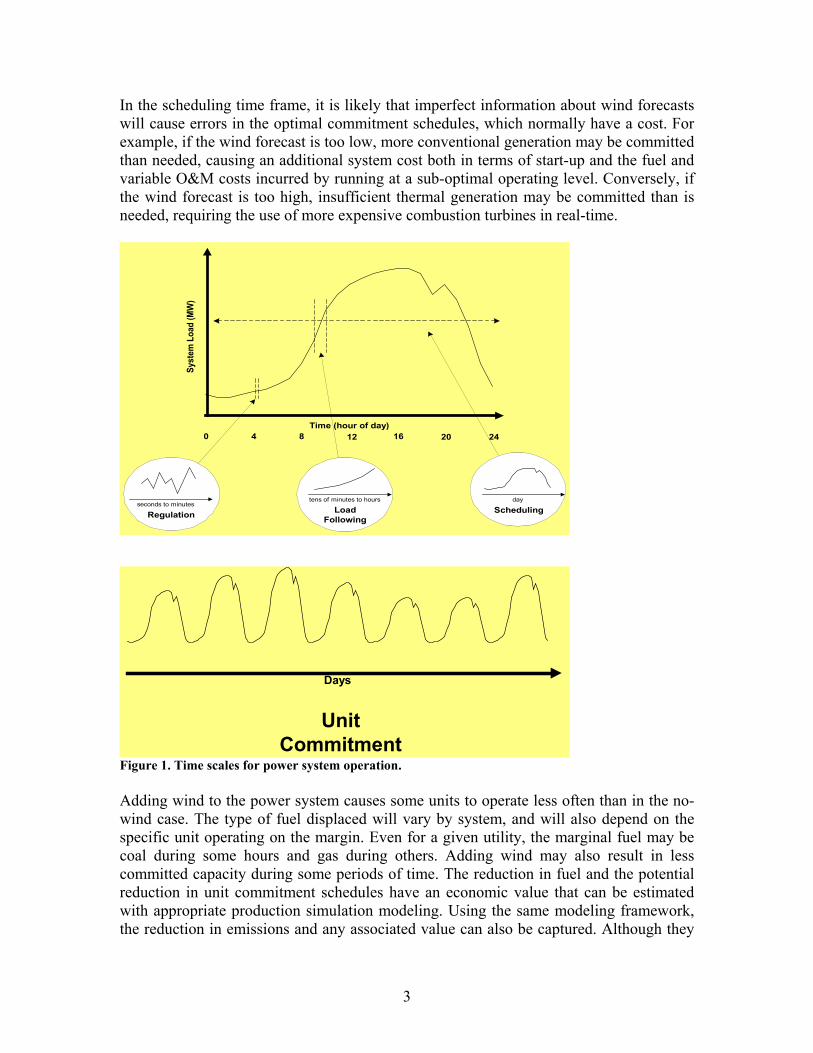
In the scheduling time frame, it is likely that imperfect information about wind forecasts will cause errors in the optimal commitment schedules, which normally have a cost. For example, if the wind forecast is too low, more conventional generation may be committed than needed, causing an additional system cost both in terms of start-up and the fuel and variable O&M costs incurred by running at a sub-optimal operating level. Conversely, if the wind forecast is too high, insufficient thermal generation may be committed than is needed, requiring the use of more expensive combustion turbines in real-time.
Time (hour of day)0 4 8 12 16 20 24
Syst
em L
oad
(MW
)
seconds to minutes
Regulation
tens of minutes to hours
LoadFollowing
day
Scheduling
Days
UnitCommitment
Figure 1. Time scales for power system operation. Adding wind to the power system causes some units to operate less often than in the no-wind case. The type of fuel displaced will vary by system, and will also depend on the specific unit operating on the margin. Even for a given utility, the marginal fuel may be coal during some hours and gas during others. Adding wind may also result in less committed capacity during some periods of time. The reduction in fuel and the potential reduction in unit commitment schedules have an economic value that can be estimated with appropriate production simulation modeling. Using the same modeling framework, the reduction in emissions and any associated value can also be captured. Although they

4
are more difficult to capture, the risks associated with fuel (availability, price, or both) and emission can be calculated as well. Wind integration cost studies typically address the cost of operating the conventional generation under the increased variability and uncertainty that are introduced by wind generators. However, when wind is added, additional low-cost energy is supplied above and beyond the no-wind case. To account for the potential energy bias of comparing cases with additional energy sources in the generation mix, a base case is typically constructed as the reference. Because the objective of a wind integration cost study is to capture the impact and cost of wind’s variability and uncertainty, the base case commonly includes a proxy resource that adds no additional variability or uncertainty to the resource mix. This proxy resource delivers a daily-equivalent flat energy block, based on the wind energy. Using this daily flat energy block in the base case, the power system is simulated for at least one year in hourly time steps, and the electricity production cost is noted. A second simulation case is run after replacing the flat energy block with the wind “as-delivered.” The difference in production cost between these cases is interpreted as one component of the integration cost. Although there are typically other cases that are run with varying degrees of wind forecast accuracy that can help estimate the cost of uncertainty, we will not discuss those in this paper (see Table 1). Table 1. Integration cost is calculated as the difference between simulation runs. Steps to calculate wind integration cost 1 Convert wind energy profile into a series of 365 daily flat energy-blocks 2 Run the production simulation model and record the production cost 3 Re-run the simulation, replacing the flat block with wind “as delivered” 4 The difference between costs in steps 2 and 3 is the integration cost If wind were not added to the system, there are clearly many alternative ways to deliver the energy that wind would have delivered. For example, in systems with significant natural gas generation on the margin, wind would displace gas, and perhaps some other fuel. In that case, one could argue that the no-wind case should use the wind-displaced natural gas, since that is the alternative to wind. Alternatively, the load serving entity (LSE) may be considering a contract to purchase energy as an alternative to wind. Again, one could argue that the wind case should be compared to the energy purchase case to determine the integration cost of wind. Although there may be many other alternatives to comparing wind and non-wind cases, most non-wind generation alternatives will be dispatched and will therefore ramp to some extent, given the type of unit and operational constraints. As a comparison alternative for a no-wind simulation case, use of a proxy generator was not thought to provide a good benchmark since additional variability would be introduced to the system. This led to the development of the daily flat energy block as the proxy unit: such a unit adds energy, but does not add any variability or uncertainty within the day. The caveat to this is that an

5
inter-day ramp was introduced, but at low to moderate wind penetration levels, this was generally insignificant. The flat proxy resource appears to have an unintended consequence, however, in the assessment of the system operational cost. In step 2 of Table 1, we see that the system is simulated with the proxy resource. In the next step, the proxy is removed and the wind is added to the model “as-delivered.” The no-wind case therefore introduces additional energy into the system. Since the energy for this resource is available as a flat block throughout the day, part of that energy is available during peak periods during which prices are generally higher than average. But for the wind case, more energy is often delivered during off-peak periods when energy prices are lower. Consequently, the differential between the simulations will introduce a difference in energy value, as distinct from an integration cost. To explore whether this is a significant issue, we set up a series of test cases. The results and discussion of these cases appears in the sections below.
Simple example: separating value from cost We used 3 years of hourly wind production data taken from the Minnesota 20% Wind Integration Study (EnerNex, 2006), along with locational marginal prices (LMP) obtained from the MISO. We used wind data from 2003, 2004, and 2005 from the Numerical Weather Prediction (NWP) modeling phase of the study, and LMPs from 2008. Unfortunately, we were unable to find LMP and wind data from the same year, so that implies that our results are only indicative. However, our findings indicate that there may be a significant value component that is unintentionally embedded in wind integration costs that are calculated using a daily flat block reference. To reinforce our basic argument, we first show the average daily profile from the 2004 wind data and the LMPs in Figure 2. Wind production can be seen to drop on average during the day, whereas energy prices generally rise in the early morning and drop off in the evening. From an aggregate annual perspective, the implication appears to be that the value of the wind energy would be somewhat less than an energy-equivalent resource that delivers a constant amount of energy during the day. We now walk through the development of a simple example to provide the context for our evaluation of the potential value differential between wind energy and the daily flat-block proxy resource.

6
MISO LMP and Wind (2004)
0
500
1000
1500
2000
2500
3000
0:00 6:00 12:00 18:00 0:00
Win
d M
W
$0
$10
$20
$30
$40
$50
$60
$70
$80
Syst
em $
/MW
H
Wind MW Average
Hourly Energy Price Average
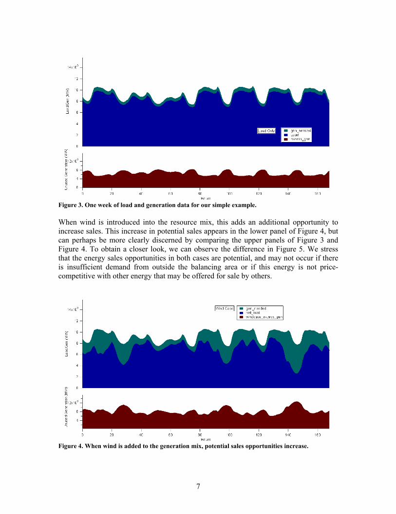
Figure 2. Prices and wind power production generally follow different diurnal patterns. We use data from the Minnesota 20% Wind Integration Study as the basis for our discussion and example calculations. To simplify the discussion, we abstract from the actual resource stack, and assume that there is sufficient generation within the state-wide balancing area to cover loads plus contingency reserves. This simplistic generalization does not have any material impact on our results or analysis. Most of the graphics we show are intended to illustrate the process, and are based on the first week of the year. However, our analysis covers one year of wind data and three years of energy price data. Figure 3 shows our base case situation. The available generation is sufficient to cover the load plus a 7% reserve margin as shown in the upper panel. Because there is excess generation that is not committed in this first week of January for this summer-peaking system, the lower panel shows the potential energy sales that could be made. The shape of this curve clearly shows the diurnal pattern of the excess generation, which tends to be higher at night and lower during the day.
7
Figure 3. One week of load and generation data for our simple example. When wind is introduced into the resource mix, this adds an additional opportunity to increase sales. This increase in potential sales appears in the lower panel of Figure 4, but can perhaps be more clearly discerned by comparing the upper panels of Figure 3 and Figure 4. To obtain a closer look, we can observe the difference in Figure 5. We stress that the energy sales opportunities in both cases are potential, and may not occur if there is insufficient demand from outside the balancing area or if this energy is not price-competitive with other energy that may be offered for sale by others.
Figure 4. When wind is added to the generation mix, potential sales opportunities increase.

8
Figure 5. Comparison of potential energy sales for the no-wind and wind cases. We now turn to a comparison of the market value of wind and the value of the flat block proxy. In our analysis, we assume that wind does not have any impact on market prices. This simplifying assumption may not be valid for high wind penetrations, especially when periods of high wind energy production coincide with low-load periods. We discuss the implication of this issue later in the paper, but they tend to increase rather than decrease the concern with the flat block proxy. The typically proxy resource, an energy-equivalent flat energy block for the day, is represented in Figure 6. The annual value of the proxy resource is $48.82/MWh. Figure 7 shows the market price, wind energy production, and wind energy value for the same time period. The annual wind energy value is $47.36/MWh. There is clearly a difference in the value with the flat energy block being worth $1.46/MWh more, on average, than the wind energy, as delivered.

9
Figure 6. One week of the daily flat energy block and market value. The annual market value of the flat block is $48.82/MWh.
Figure 7. One week of market price, wind energy, and wind market value. Annual wind value is $47.36/MWh.

10
Because the daily flat block cannot distinguish between high-price and low-price periods, which tend to cycle by time of day, we performed a simple comparison of the daily flat energy-block value to the value of a 6-hour block. As might be expected, the 6-hour flat block more closely matches the wind than does the daily flat block. Figure 8 provides an example. The upper panel shows the daily block, along with the hourly wind generation and hourly LMP. In the lower panel, the wind and LMP traces are replicated for convenience, and the 6-hour flat block replaces the daily block.
Figure 8. The 6-hour flat block does a better job of approximating wind energy value than the daily block. The comparative values are displayed in Figure 9. In both panels, the red line (scale to the right) indicates the divergence of the block’s value from the wind value. The graph shows that the divergence of value varies considerably by hour, but for the full year of 2004 the daily block is $1.46/MWh higher than the wind value, whereas the 6-hour flat block is only $0.23/MWh higher than the wind value.

11
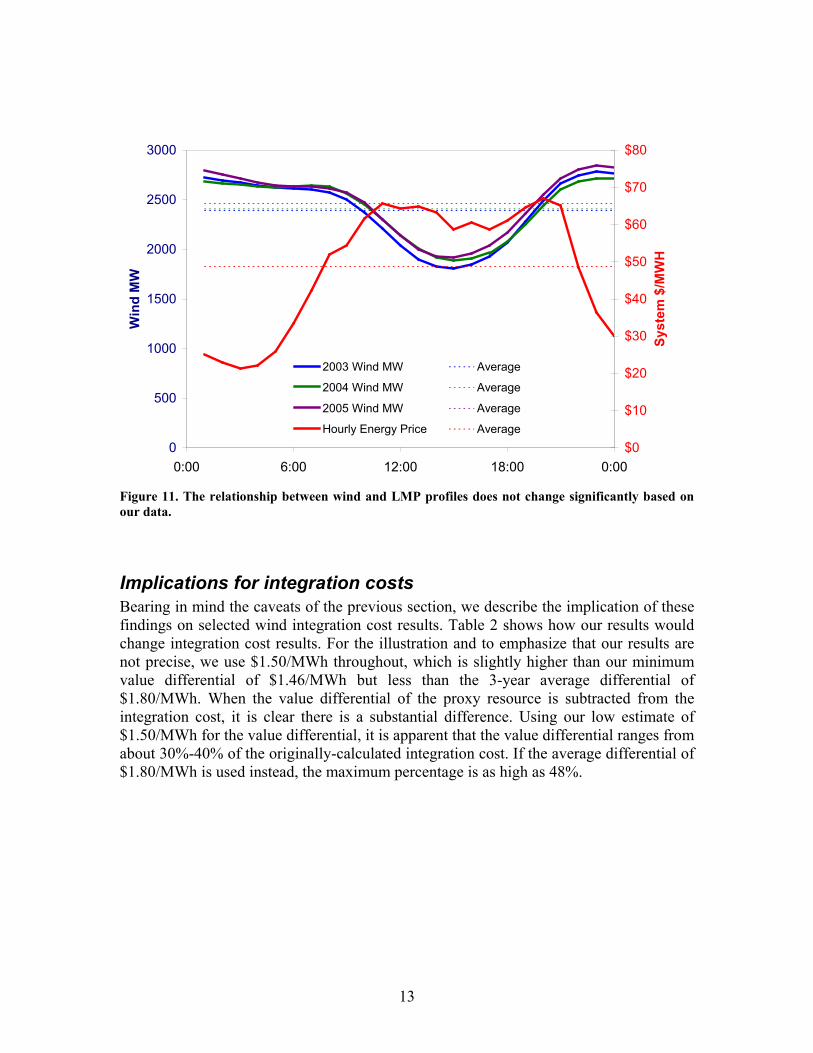
Figure 9. The 6-hour flat block comes closer to estimating wind's value than the daily flat block. This result also applies to the three years of wind data we analyzed. In all cases, the 6-hour block value came closer than the daily block value. Figure 10 shows these results as differences from the wind case. For example in 2003 the daily block value is nearly $2.00/MWh more than the wind value, but the 6-hour block is $0.23/MWh higher in value than the wind. Examining the average profiles for the 3-year wind data set alongside the average LMP profile in Figure 11 shows that the basic relationship of the diurnal wind profiles to LMP does not change significantly from year to year.
Discussion and Caveats Given that our LMP and wind data come from different years, we believe our results to be illustrative of the fact that the differential energy value of a daily flat block compared to wind energy is inadvertently included in the integration cost, as measured in several wind integration cost studies. Our particular numerical results are significant in the sense that they illustrate the magnitude of the problem, but they should not be treated as precise estimates of the value differential. It is important to stress the caveats to this analysis. First, we assume that wind is a perfect price-taker in the energy market. Under this assumption, wind has no influence or impact on LMP. Although this is likely true at low penetration rates when transmission congestion is not an issue, it does not hold in cases of very high wind penetration or significant congestion. Evidence from large-scale integration studies (for example California Energy Commission, 2007)shows that wind can cause market prices to fall at

12
high penetrations. The potential sensitivity of LMP to wind injections should only provide a wider spread to the value differentials we have identified. The wind and price data in our analysis comes from different years. As can be seen in Figure 11, the average diurnal profiles of wind do not appear to vary significantly in comparison to the LMP profile. We expect our results are indicative of the value differential between wind and daily flat energy blocks, but are not precise. We also expect that the value differentials would likely vary for different utilities and markets, and different wind penetrations.
0.00
0.50
1.00
1.50
2.00
2.50
2003 2004 2005
Mar
ket V
alue
Diff
eren
ce fr
om W
ind
($/M
Wh)
Daily less wind6-hour less wind
Figure 10. 3-year results summary.
13
0
500
1000
1500
2000
2500
3000
0:00 6:00 12:00 18:00 0:00
Win
d M
W
$0
$10
$20
$30
$40
$50
$60
$70
$80
Syst
em $
/MW
H
2003 Wind MW Average
2004 Wind MW Average
2005 Wind MW Average
Hourly Energy Price Average
Figure 11. The relationship between wind and LMP profiles does not change significantly based on our data.
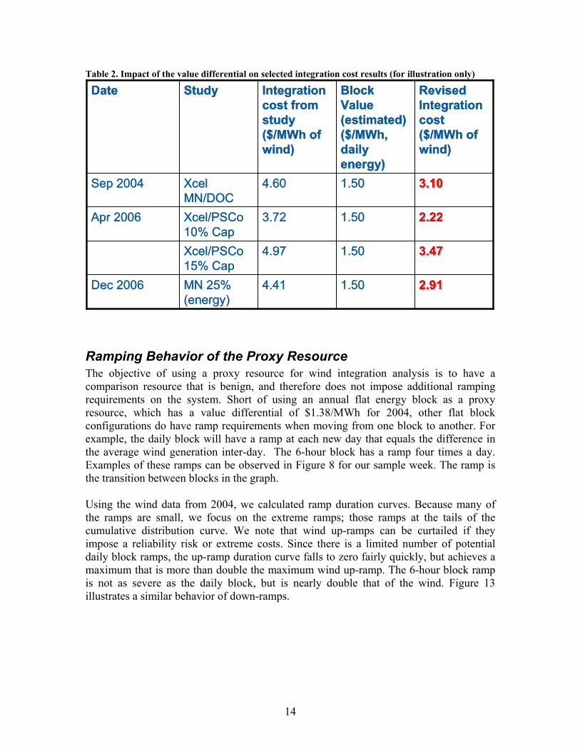
Implications for integration costs Bearing in mind the caveats of the previous section, we describe the implication of these findings on selected wind integration cost results. Table 2 shows how our results would change integration cost results. For the illustration and to emphasize that our results are not precise, we use $1.50/MWh throughout, which is slightly higher than our minimum value differential of $1.46/MWh but less than the 3-year average differential of $1.80/MWh. When the value differential of the proxy resource is subtracted from the integration cost, it is clear there is a substantial difference. Using our low estimate of $1.50/MWh for the value differential, it is apparent that the value differential ranges from about 30%-40% of the originally-calculated integration cost. If the average differential of $1.80/MWh is used instead, the maximum percentage is as high as 48%.
14
Table 2. Impact of the value differential on selected integration cost results (for illustration only)
1.50
1.50
1.50
1.50
Block Value (estimated) ($/MWh, daily energy)
2.914.41MN 25% (energy)
Dec 2006
3.474.97Xcel/PSCo15% Cap
2.223.72Xcel/PSCo10% Cap
Apr 2006
3.104.60Xcel MN/DOC
Sep 2004
Revised Integration cost ($/MWh of wind)
Integration cost from study ($/MWh of wind)
StudyDate
1.50
1.50
1.50
1.50
Block Value (estimated) ($/MWh, daily energy)
2.914.41MN 25% (energy)
Dec 2006
3.474.97Xcel/PSCo15% Cap
2.223.72Xcel/PSCo10% Cap
Apr 2006
3.104.60Xcel MN/DOC
Sep 2004
Revised Integration cost ($/MWh of wind)
Integration cost from study ($/MWh of wind)
StudyDate
Ramping Behavior of the Proxy Resource The objective of using a proxy resource for wind integration analysis is to have a comparison resource that is benign, and therefore does not impose additional ramping requirements on the system. Short of using an annual flat energy block as a proxy resource, which has a value differential of $1.38/MWh for 2004, other flat block configurations do have ramp requirements when moving from one block to another. For example, the daily block will have a ramp at each new day that equals the difference in the average wind generation inter-day. The 6-hour block has a ramp four times a day. Examples of these ramps can be observed in Figure 8 for our sample week. The ramp is the transition between blocks in the graph. Using the wind data from 2004, we calculated ramp duration curves. Because many of the ramps are small, we focus on the extreme ramps; those ramps at the tails of the cumulative distribution curve. We note that wind up-ramps can be curtailed if they impose a reliability risk or extreme costs. Since there is a limited number of potential daily block ramps, the up-ramp duration curve falls to zero fairly quickly, but achieves a maximum that is more than double the maximum wind up-ramp. The 6-hour block ramp is not as severe as the daily block, but is nearly double that of the wind. Figure 13 illustrates a similar behavior of down-ramps.

15
National Renewable Energy Laboratory Innovation for Our Energy FutureNational Renewable Energy Laboratory Innovation for Our Energy Future
Up ramps can be mitigated (curtailed) if they impose a high cost or reliability risk.
Figure 12. Extreme up-ramps from the flat blocks exceed wind ramps.
Figure 13. Extreme down-ramps from the flat block exceed wind ramps.

16
Case Study: Eastern Wind Integration and Transmission Study The National Renewable Energy Laboratory is currently managing a large-scale wind integration study known as the Eastern Wind Integration and Transmission Study (EWITS). The study is sponsored by the U.S. Department of Energy, and is coordinated with the Joint Coordinated System Plan (www.jcspstudy.org) analysis that is hosted by the MISO. The study examines the impact of several wind build-out scenarios that achieve a 20% energy penetration within the study footprint, shown in Figure 14. One scenario examines a 30% wind energy penetration. In some of the early modeling work for EWITS that was carried out by teams at Ventyx and EnerNex, very large inter-day ramps were found in the daily flat-block proxy modeling cases. As a result, the project team spent some time discussing the issue and examining alternative approaches. Although it is premature to discuss specific findings of the EWITS analysis since work is ongoing, we include some discussion surrounding the proxy resource and additional alternatives.3
Figure 14. Footprint of the Eastern Wind Integration and Transmission Study.
3 Thanks to Jack King, EnerNex, for providing data and processing.

17
To address the large inter-day ramps imposed by the daily flat block proxy resource, several alternatives were suggested. These include the 6-hour flat block, along with rolling averages of 24, 48, 96, and 168 hours (one week), respectively. In addition, a 3-year flat block was tested since that has no ramp characteristic at all. Using wind data from 2004-2006 and LMPs from 2008, as before, we analyzed the market value of wind energy and each of these alternative proxy resources. While the rolling average proxy methods do eliminate the inter-day ramping concerns, we found little difference in the market value of all of the rolling average proxies and the daily flat block. The 6-hour fixed block was the closest to wind of all proxy resources we examined. The 3-year flat block commanded a higher value than any of the alternatives. The results are presented graphically in Figure 15, which also shows the market value differential of each of the proxy resources. In most cases, the differential is approximately $1.70/MWh of wind, although the 3-year block value is more than $2.00/MWh higher than wind. We also show ramp duration curves for selected proxy resources: daily block, and 24-hour moving average. Figure 16 shows that most ramps are within a range of plus-minus 4,000 MW/hour. We stress that the wind scenario represents approximately 300,000 MW of installed wind capacity across most of the footprint of the Eastern Interconnection, so 4,000 MW/hour is not excessive. However, we are more interested in the extreme ramp impacts. Figure 17 zooms in on the left side of Figure 16 and shows that the daily block nearly triples the maximum up-ramp compared to wind in the 3-year data set. The 24-hour moving average appears much more benign, and is potentially of interest as a proxy resource if the market value can be properly accounted for in integration analyses. The down-ramp characteristics of these proxies and wind are nearly symmetrical. Figure 18 re-scales the 24-hour moving average ramp duration, and shows that the maximum and minimum ramps are 2,284 and -2,261 MW/hour, respectively.

18
Value Comparison
45.50
46.00
46.50
47.00
47.50
48.00
48.50
49.00
wind 24-hour 48-hour 96-hour 168-hour 6-hourfixed
daily fixed 3-yr flat
$/M
Wh
Figure 15. Market value and differential value of alternative proxy resources.

19
Figure 16. 3-year ramp duration curve shows many hours of relatively small ramps.

20
Figure 17. Extreme up-ramps occur in the daily flat block compared to wind, but the 24-hour moving average appears much more benign.
Figure 18. Duration curve for the 24-hour moving average proxy.

21
The 168-hour moving average has a significant smoothing effect on hourly ramps. It appears to be promising as a benchmark resource. The one-week moving average ramp duration curve appears in Figure 19 and shows that the ramps all fall within the range of -353 MW/hour to 381 MW/hour.
Figure 19. A 168-hour (1 week) moving average proxy has very little ramp from hour to hour. However, there is still a lot of variability that exists in the 168-hour moving average, as indicated in Figure 20, and in a more detailed representation in Figure 21.

22
Figure 20. Zooming in on the first 3,000 hours shows the variability in the 168-hour moving average.
Figure 21. Zooming in on the first 3,000 hours of the 168-hour moving average shows the pattern of variability and ramp characteristics.

23
Discussion of Proxy Resource Issues Using a fixed flat energy block as a proxy resource for wind integration cost analysis introduces significant inter-day ramps at high penetrations. These ramps are not real, nor do they provide a firm basis for a comparison/proxy resource at moderate to high wind penetrations. The impact of these artificial ramps is expected to vary depending on the size of the ramp and the position of generating units in the dispatch stack at the block boundaries (such as the 6-hour or 24-hour times of day). At lower penetrations, this impact may be more moderate, but could still be significant, mimicking the behavior of 1-hour block energy schedules that are still widely used in the Western Interconnection. All of the proxy methods examined here have a significant market-value component that contributes to integration cost estimates. This intertwines the integration cost with an energy value differential that is not real—it is an artifact of the constructed proxy resource. This differential can in principle be removed from the analysis, using the appropriate LMPs from each of the modeling cases: the proxy resource case and the wind case.
Conclusions As larger and larger amounts of wind generation are installed, we increasingly gain environmental and fuel savings benefits. Along with these benefits, there are costs that result from wind variability and uncertainty. Wind integration costs cannot be calculated directly. Instead, the power system is simulated with and without wind generation, and the difference in total system costs is attributed to wind integration. A proxy energy source that does not include variability or uncertainty must be included in the “without wind” case or else wind integration costs would be credited with the wind energy itself. Finding an appropriate proxy energy source is surprisingly difficult. Selecting an appropriate non-varying and non-uncertain proxy energy source is difficult because any difference in the value of the proxy energy and the wind energy shows up in the calculated wind integration cost. A daily flat-block energy schedule that matches the daily wind energy output seems ideal because it is both certain and steady. Unfortunately, the daily flat block tends to have more on-peak energy and less off-peak energy than the wind itself. Consequently, the daily flat block is worth $1.50-$2.00/MWh more than the actual wind energy. Wind integration studies that utilize the flat daily block overstate wind integration costs. Daily flat blocks also can have large step changes at midnight. These step changes result in artificial ramping requirements that the real power system never sees. Rolling averages of 24 to 168 hours can be used to eliminate the step changes. These rolling averages still have the problem that the proxy energy value is higher than the actual wind energy value. While we hoped to develop an ideal proxy energy resource to use in wind integration studies, we found that the problem is over specified. The proxy must be unvarying, certain, and of the same value as the actual wind. Meeting the certainty and value requirements simultaneously is not strictly possible. It does not appear to be possible to relax the two requirements slightly and develop a solution that is adequate for

24
engineering studies. The best solution may be to use a 24-hour rolling average to provide certainty and near invariability, while eliminating artificial ramps at midnight that are associated with the daily flat blocks. The difference in energy value must then be backed out of the calculated integration cost.
References Charlie Smith, Michael Milligan and Brian Parsons, Ed DeMeo (2007), Utility Wind Integration State of the Art. IEEE Transactions on Power Systems. Aug. Posted with permission at http://www.nrel.gov/docs/fy07osti/41329.pdf. California Energy Commission (2007) California Intermittency Analysis Project. Available: www.uwig.org EnerNex, (2006). Final Report - 2006 Minnesota Wind Integration Study Volume I. http://www.uwig.org/windrpt_vol%201.pdf.

F1147-E(10/2008)
REPORT DOCUMENTATION PAGE Form Approved OMB No. 0704-0188
The public reporting burden for this collection of information is estimated to average 1 hour per response, including the time for reviewing instructions, searching existing data sources, gathering and maintaining the data needed, and completing and reviewing the collection of information. Send comments regarding this burden estimate or any other aspect of this collection of information, including suggestions for reducing the burden, to Department of Defense, Executive Services and Communications Directorate (0704-0188). Respondents should be aware that notwithstanding any other provision of law, no person shall be subject to any penalty for failing to comply with a collection of information if it does not display a currently valid OMB control number. PLEASE DO NOT RETURN YOUR FORM TO THE ABOVE ORGANIZATION. 1. REPORT DATE (DD-MM-YYYY)
July 2009 2. REPORT TYPE
Technical Report 3. DATES COVERED (From - To)
4. TITLE AND SUBTITLE
Calculating Wind Integration Costs: Separating Wind Energy Value from Integration Cost Impacts
5a. CONTRACT NUMBER DE-AC36-08-GO28308
5b. GRANT NUMBER
5c. PROGRAM ELEMENT NUMBER
6. AUTHOR(S) M. Milligan and B. Kirby
5d. PROJECT NUMBER NREL/TP-550-46275
5e. TASK NUMBER WER95501
5f. WORK UNIT NUMBER
7. PERFORMING ORGANIZATION NAME(S) AND ADDRESS(ES) National Renewable Energy Laboratory 1617 Cole Blvd. Golden, CO 80401-3393
8. PERFORMING ORGANIZATION REPORT NUMBER NREL/TP-550-46275
9. SPONSORING/MONITORING AGENCY NAME(S) AND ADDRESS(ES)
10. SPONSOR/MONITOR'S ACRONYM(S) NREL
11. SPONSORING/MONITORING AGENCY REPORT NUMBER
12. DISTRIBUTION AVAILABILITY STATEMENT National Technical Information Service U.S. Department of Commerce 5285 Port Royal Road Springfield, VA 22161
13. SUPPLEMENTARY NOTES
14. ABSTRACT (Maximum 200 Words) Accurately calculating integration costs is important so that wind generation can be fairly compared with alternative generation technologies.
15. SUBJECT TERMS Wind; grid integration; systems integration; capacity credit; integration costs; wind energy value, electric system; wind power; utility
16. SECURITY CLASSIFICATION OF: 17. LIMITATION OF ABSTRACT
UL
18. NUMBER OF PAGES
19a. NAME OF RESPONSIBLE PERSON a. REPORT
Unclassified b. ABSTRACT Unclassified
c. THIS PAGE Unclassified 19b. TELEPHONE NUMBER (Include area code)
Standard Form 298 (Rev. 8/98) Prescribed by ANSI Std. Z39.18