Calculating and Synthesizing Effect Sizes for Single-Subject Experimental

Designs

NCDDR's 2009/10 Course: Conducting Systematic Reviews of Evidence-Based Disability and Rehabilitation ResearchApril 28, 2010

Oliver Wendt, PhD Purdue University

Single-subject Experimental Designs (SSEDs) Examining pre- versus post-treatment perfor- mance

within a small sample (Kennedy, 2005) Experimental approach reveal causal relationship

between IV and DV Employs repeated and reliable measurement, within- and

between-subject comparisons to control for major threats to internal validity

Requires systematic replication to enhance external validity

Basis for determining treatment efficacy, used to establish evidence-based practice (Horner et al., 2005)

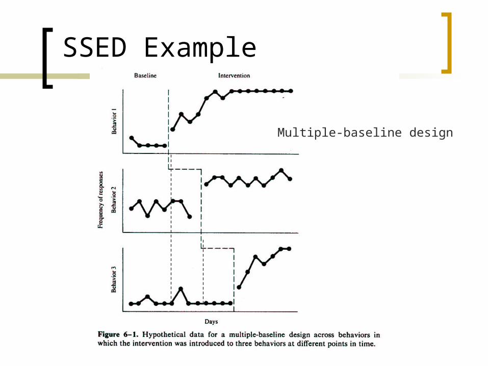
SSED Example

Multiple-baseline design

Why Effect Sizes for Single-Subject Experiments?

Single-subject experimental designs (SSEDs) traditionally evaluated by visual analysis Evidence-based practice (EBP) emphasizes

importance of more objective outcome measures, especially “magnitude of effect” indices or “effect sizes” (ES) (Horner et al., 2005).

Meta-analysis: ES are needed to summarize outcomes from SSEDs for research synthesis SSEDs predominant with low-incidence populations

Meta-analysis of SSEDs emphasized in evidence hierarchies

An Adapted Hierarchy of Evidence for Low-Incidence Populations

(Wendt & Lloyd, 2005)

1. Meta-analysis of (a) single-subject experimental designs, (b) quasi-experimental group designs (i.e., non-randomized) 2a. quasi-experimental group designs*

2b. Single-subject experimental design – one intervention

2c. Single-subject experimental design – multiple interventions

3. Quantitative reviews that are non meta-analytic 4. Narrative reviews 5. Pre-experimental group designs and qualitative case studies 6. Respectable opinion and/or anectodal evidence * Consider differences in quality regarding threats to internal and external validity (Campbell & Stanley, 1963). Adapted from Schlosser, 2003.

Current Status What “effect size metrics” are most

appropriate to measure effect size while respecting the characteristics of SSEDs

Regression-based approaches Piece-wise regression procedure (Center, Skiba,

& Casey, 1986) 4-parameter model (Huitema & McKean, 2000;

Beretvas & Chung, 2008) Multilevel Models (Van den Noortgarte &

Onghena, 2003a, 2003b) Non-regression-based approaches

Family of “non-overlap” metrics Specific metrics for behavior increase versus

behavior reduction data

Group vs. SSED Effect Sizes

Group designs and single subject research designs have different effect size metrics

THESE CANNOT BE COMBINED! Group designs conventionally employ:

d family effect sizes including the standardized mean difference magnitude (e.g., Cohen’s d, Hedges’ g)

r family effect sizes including correlation coefficients OR (odds ratio) family effect sizes including

proportions and other measures for categorical data

General Considerations and Precautions

Requirements of the specific metric applied Minimum number of data points or participants Specific type of SSED (e.g., multiple baseline) Randomization (e.g., assignment to treatment

conditions, order of participants) Assumptions of data distribution and nature

(e.g., normal distribution, no autocorrelation) Limitations

Ability to detect changes in level and trend Orthogonal slope changes Sensitivity to floor and ceiling effects

Direction of behavior change Behavior increase vs. decrease

Orthogonal Slope Changes

Non-regression Based Approaches Family of “non-overlap” metrics

Improvement Rate Difference (IRD) Non-overlap of All Pairs (NAP) Percentage of Non-overlapping Data (PND) Percentage of All Non-overlapping Data (PAND) Percentage of Data Points Exceeding the Median

(PEM) Percentage of Data Points Exceeding a Median

Trend (PEM-T) Pair-wise Data Overlap (PDO)

Specific metrics for behavior reduction data (vs. behavior increase data) Percentage Reduction Data (PRD) Percentage of Zero Data (PZD)

Percentage of Nonoverlapping Data (PND)

Calculation of non-overlap between baseline and successive intervention phases (Scruggs, Mastropieri, & Casto, 1987)

Identify highest data point in baseline and determine the percentage of data points during intervention exceeding this level

Easy to interpret Non-parametric statistic

PND Calculation: An Example

PND = 11/15 = .73 or 73%

Interpretation of PND Scores If a study includes several experiments,

PND scores are aggregated by taking the median (rather than mean)

Scores usually not distributed normally Median less effected by “outliers”

PND statistic: the higher the percentage the more effective the treatment

Specific criteria for interpreting PND scores outlined by Scruggs, Mastropieri, Cook, and Escobar (1986)

Interpretation of PND Scores (cont.)

PND range 0-100% PND < 50% reflects unreliable treatment PND 50% - 70% questionable effectiveness PND 70% - 90% fairly effective PND > 90% highly effective

Limitations of PND

Ignores all baseline data except one data point (this one can be unreliable)

Ceiling effects Lacks sensitivity or discrimination ability

as it nears 100% for very successful interventions

Can not detect slope changes Needs its own interpretation guidelines

Technically not an effect size

Percentage of All Non-Overlapping Data (PAND)

Calculation of total number of data points that do not overlap between baseline and intervention phases (Parker, Hagan-Burke, & Vannest, 2007) Identify overlapping data points (minimum

number that would have to be transferred across phases for complete data separation)

Compute % overlap by dividing number of overlapping points by total number of points

Subtract this percent from 100 to get PAND

Non-parametric statistic

PAND Calculation: An Example

PAND = 23/25 = .92 or 92%

% Overlap = 2/25 = 8%PAND = 100%-8%= 92%

Advantages of PAND

Uses all data points across both phases

May be translated to Phi and Phi² to determine effect size (e.g., Cohen’s d)

Limitations of PAND

Insensitive at the upper end of the scale 100% is awarded regardless of distance

between data points in the two phases Measures only mean level shifts and

does not control for positive baseline trend

Requires 20 data points for calculation (if attempt to calculate Phi statistic)

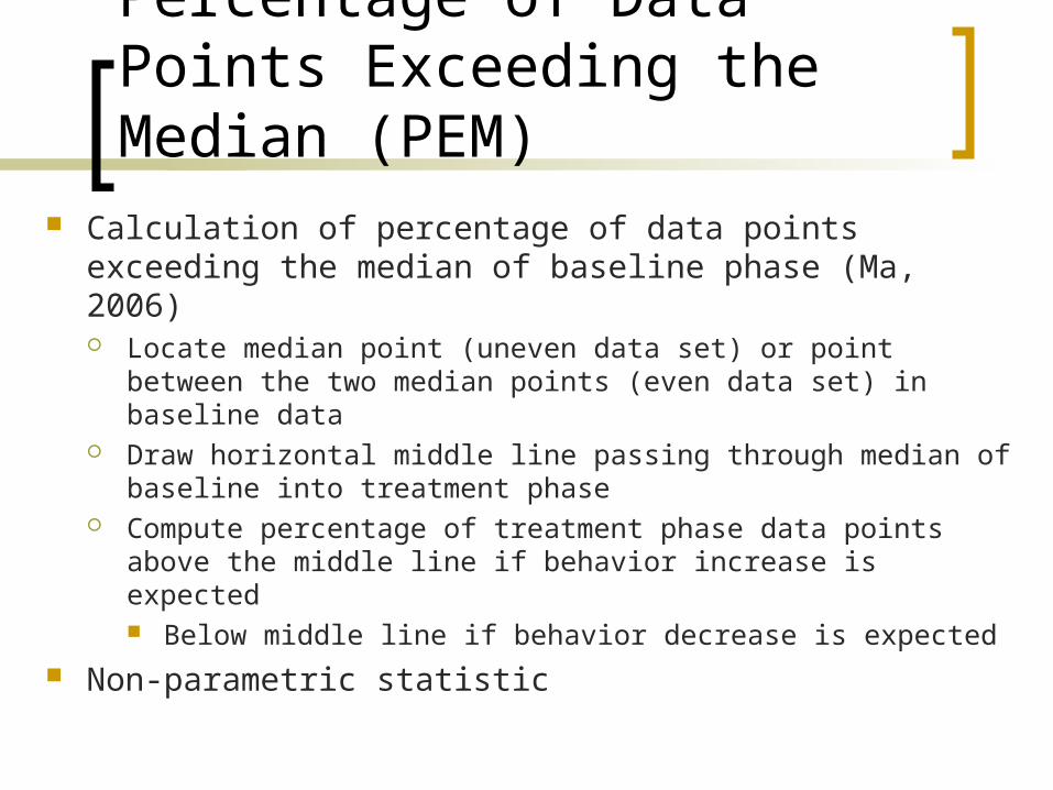
Percentage of Data Points Exceeding the Median (PEM)

Calculation of percentage of data points exceeding the median of baseline phase (Ma, 2006) Locate median point (uneven data set) or point between

the two median points (even data set) in baseline data Draw horizontal middle line passing through median of

baseline into treatment phase Compute percentage of treatment phase data points above

the middle line if behavior increase is expected Below middle line if behavior decrease is expected

Non-parametric statistic

PEM Calculation: An Example

PEM = 15/15 = 1 or 100%

Interpretation of PEM

Null hypothesis If treatment is ineffective, data points will

continually fluctuate around the middle line PEM scores range from 0 to 1

.9 to 1 reflects highly effective treatment .7 to .9 reflects moderately effective

treatment Less than .7 reflects questionable or not

effective treatment

Advantages of PEM

In the presence of floor or ceiling data points, PEM still reflects effect size while PND does not

Limitations of PEM

Insensitive to magnitude of data points above the median

Does not consider trend and variability in data points of treatment phase

May reflect only partial improvement if orthogonal slope is present in baseline treatment pair after first treatment phase

Pairwise Data Overlap (PDO) Calculation of overlap of all possible paired

data comparisons between baseline and intervention phases (Parker & Vannest, in press) Compare baseline data point with all intervention

data points Determine number of overlapping (ol) and non-

overlapping (nol) points Compute total number of “nol” points divided by

total number of comparisons Non-parametric statistic

PDO Calculation: An Example

PDO = (15+15+15+14+15+11+15+15+15+15)/(15x10) = .97 or 97%

Advantages and Limitations of PDO

Produces more reliable results as other non-parametric indices

Relates closely to established effect sizes (Pearson R, Kruskal-Wallis W)

Takes slightly longer to calculate Requires that individual data point

results be written down and added Calculation is laborious for long and

crowded data series

Non-overlap of All Pairs (NAP) Another way of summarizing data overlap

between each phase A datapoint and each phase B datapoint (Parker & Vannest, 2009) A non-overlapping pair will have a phase B data

point larger than its paired baseline B datapoint NAP reflects the number of comparison pairs

showing no overlap, divided by the total number of comparisons

Non-parametric statistic

NAP Calculation: An ExampleNAP = (10 x 11) - (0 + 0 + 0 + 0 + 0 + 3 + 1 + 0 + 0 + 0) / (10 x 11) = 106/110 = 96%

Advantages and Limitations of NAP

Accounts for “ties” when assessing overlapping data points

Strong discriminability Closely related to established effect size

R2; But Like PDO: Takes slightly longer to calculate Requires that individual data point

results be written down and added Calculation can be laborious

Improvement Rate Difference (IRD)

Calculation of percentage of improvement between baseline and intervention performance (Parker, Vannest, & Brown, 2009)

Identify minimum number of data points from baseline and intervention that would have to be removed for complete data separation

Points removed from baseline are “improved” (overlap with intervention) and points removed from intervention are “not improved” (overlap with baseline)

Subtract % “improved” in baseline from % “improved” in treatment

Improved

IRD: An Example

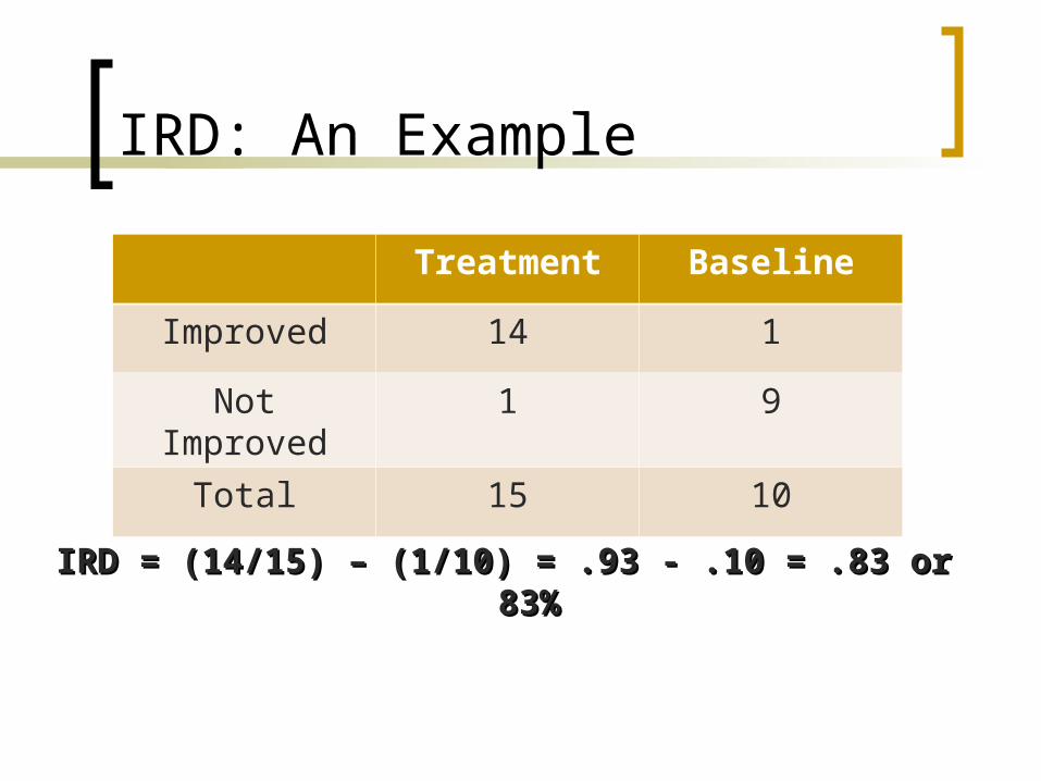
Treatment Baseline

Improved 14 1

Not Improved 1 9

Total 15 10

IRD: An Example

IRD = (14/15) – (1/10) = .93 - .10 = .83 or 83%IRD = (14/15) – (1/10) = .93 - .10 = .83 or 83%

Advantages of IRD

Provides separate improvement rates for baseline and intervention phases

Better sensitivity than PND Allows confidence intervals Proven in medical research

Limitations of IRD

Conventions for calculation not always clear for more complex and multiple data series

“Baseline improvement” misleading concept

Needs validation and comparison to existing measures

Percentage of Data Exceeding a Median Trend (PEM-T) Uses the split-middle technique (White & Haring,

1980), a common approach to determine trend in SSED data, as a cut-off for non-overlap

Calculation of percentage of data points exceeding the trend line (Wolery et al., 2010) Calculate and draw the split middle line of trend

through phase A and extend to phase B Count the number of data points in phase B

above trend line and calculate percentage of non-overlap

Non-parametric statistic

PEM-T Calculation: An ExamplePEM-T = 0/10 = 0% (behavior increase)PEM-T = 10/10 = 100% (behavior increase)

Limitations and Benefits of PEM-T

Poor agreement with visual analysis Better than other metrics in terms of

total error percentage but still errors in 1/8 of all data

Can detect changes in level but cannot detect changes in variability (none of the others can either)

How Do PND, PEM, PAND, PDO and IRD Compare?

All five effect size metrics were applied to “real data”

Data set taken from systematic review of school-based instructional interventions for students with autism spectrum disorders (Machalicek et al., 2008)

Outcomes: communication skills (e.g., gestures, natural speech, use of speech-generating device)

N=9 studies, 24 participants, various designs, 72 A-B phases (acquisition) extracted

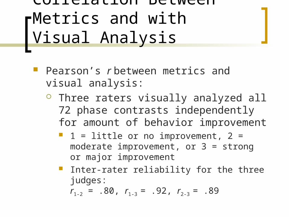
Correlation Between Metrics and with Visual Analysis

Pearson’s r between metrics and visual analysis: Three raters visually analyzed all 72

phase contrasts independently for amount of behavior improvement 1 = little or no improvement, 2 = moderate

improvement, or 3 = strong or major improvement

Inter-rater reliability for the three judges: r1-2 = .80, r1-3 = .92, r2-3 = .89

ResultsCorrelations between non-parametric effect size indices and visual analysis (VA)

PND PEM PAND PDO2 IRD VA

PND 1 .790* .764* .914* .869* .900*

PEM .790* 1 .828* .931* .818* .840*

PAND .764* .828* 1 .806* .757* .784*

PDO2 .914* .931* .806* 1 .911* .871*

IRD .869* .818* .757* .911* 1 .819*

VA .900* .840* .784* .871* .819* 1

* Correlation is significant at the .01 level (2-tailed)

Ability to Discriminate Among Chosen Studies

Usefulness of any new ES metric will depend in part on its ability to discriminate among results from published studies.

Uniform probability distribution can indicate good discriminability by plotting ES values on the y-axis versus percentile ranks on the x-axis

Shape of the obtained score distribution serves as an indicator for discriminability: ideal distributions appear as diagonal lines, without floor or ceiling effects, and without gaps, lumping, or flat segments (Chambers, Cleveland, Kleiner, & Tukey, 1983).

Discriminability: Uniform Probability Plot

0.0

33.3

66.7

100.0

0.0 0.3 0.7 1.0

Uniform Probability Plot

Percentile Rank

Eff

ect

Siz

e

0.0

33.3

66.7

100.0

0.0 0.3 0.7 1.0

Uniform Probability Plot

Percentile Rank

Eff

ect

Siz

e

Variables

PNDPEMPANDPDOIRD

Observed Patterns: PEM/PND versus PAND

(Buffington et al., 1998)

Observed Patterns: PEM Inflated Scores

PND

PEM

Hetzroni & Shalem, 2005

Observed Patterns: PND Distorted by Outliers

Keen, Sigafoos, & Woodyatt, 2001

Observed Patterns: PAND, PEM, PND Insensitivity

PAND=PEM=PND= 100%

PAND=PEM=PND= 100%

Need For Better Conventions: IRD

Misleading ES Estimates: PAND Example

PAND reports an improvement in target behavior when no improvement is observed

Recommendations Behavior Increase Data

Start with PND because Most widely established metric Known and validated interpretational guidelines

Document instances where you think PND score is problematic (e.g., ceiling effect, too much variability in the data)

Supplement PND with newer metric PAND for multiple-baseline designs IRD, but need to give conventions NAP ? May be worth trying

Percentage Reduction Data (PRD) Calculation of reduction of targeted

behavior due to intervention (O’Brien & Repp, 1990) Determine mean of last three data points

from baseline (µB) and of last three data points from intervention (µI)

Calculate the amount of change between baseline and treatment [(µB - µI) ÷ µB] x 100

Also called Mean Baseline Reduction (MBR) (Campbell, 2003, 2004)

Baseline (B) Intervention (I)

µB = (52 + 23 + 45)/3 = 40µI = (10 + 2+ 0)/3 = 4PRD = (40 - 4)/40 = 90%

PRD Calculation: An Example

Percentage of Zero Data (PZD)

Calculation of the degree to which intervention completely suppresses targeted behavior (Scotti et al., 1991) Identify first data point to reach zero in an

intervention phase Calculate the percentage of data points

that remain at zero from the first zero point onwards

Baseline (B) Intervention (I)

PZD = 2/6 = 33%

PZD Calculation: An Example

Interpretation of PZD scores

PZD range 0-100% PZD < 18% reflects ineffectiveness PZD 18% - 54% reflects questionable

effectiveness PZD 55% - 80% reflects fair effectiveness PZD > 80% reflects high effectiveness

How Do PND, PRD, and PZD Compare?

All three effect size metrics were applied to “real data”

Data set taken from systematic review of intervention studies on Functional Communication training (Chacon, Wendt, & Lloyd, 2006)

Intervention: graphic symbols, manual signs, speech

Study N Condition Intervention PND (%) PRD (%) PZD (%)

Braithwaite & Richdale (2000)

1 Access Vocalizations (“I want ___ please”) 100 100 95

Escape Vocalizations (“I need help please”) 92 100 100

Day, Horner, & O’Neill (1994)

1 Access Manual signs (“want”) 100 100 67

Escape Vocalizations (“go”) 100 98 50

Horner & Day (1991)

1 Escape Graphic symbol (“break”) with 1s delay

100 83 80

Graphic symbol (“break”) with 20s delay

0 -64 0

Schindler & Horner (2005)

2 Escape Graphic symbol/Vocalization (“help”)

18 83 47

Escape Graphic symbol (“change,” “activity”)

72 92 24

Sigafoos & Meikle (1996)

2 Attention Vocalizations (“Beth”) 86 81 80

Access Vocalizations (“drink,” “toy,” “want”)

100 100 96

Attention Gestures (tapping teacher’s hand) 100 100 100

Access Graphic symbols (“food,” “drink,” “toy”)

100 100 100

Wacker et al. (1990)

1 Access Gestures (touching chin) 50 49 25

Recommendations Behavior Decrease Data

Do not use PND May obtain score of 100% but significant portion of

target behavior still remaining Be clear about the different concepts that

PRD and PZD measure PRD: REDUCTION of target behavior to … degree PZD: TOTAL SUPPRESSION

Clarify nature of target behavior, treatment goal and chose PZD or PRD accordingly Ex.: smoking versus stuttering

Regression-based Approaches

Newer Approaches: 4-parameter model

(Huitema & McKean, 2000) Multilevel Models

Hierarchical Linear Models (HLM) for combining SSED data (Van den Noortgarte & Onghena, 2003a, 2003b)

Regression-based Approaches Illustration

0

5

10

15

20

25

30

0 1 2 3 4 5 6 7 8 9 10 11 12 13 14

Time

Ou

tco

me

Change in levelBaseline trend

Intervention trend and slope change

4-parameter ModelHuitema & McKean (2000)

Huitema & McKean (2000) modified Center et al.’s (1986) piecewise regression equation Introduction regression coefficients that can be used to

describe change in intercept and in slope from Baseline to Treatment phase

where

Yt = outcome score at time t

Tt = time/session point D = phase (A or B)

n1 = # time points in baseline (A)

tttttt eDnTDTY )]1([ 13210

4-parameter Model (cont.)

0 = baseline intercept (i.e., Y at time = 0)

1 = baseline linear trend (slope over time)

2 = difference in intercept predicted from treatment phase data from that predicted for time = n1+1 from baseline phase data

3 = difference in slope

Thus, 2 and 3 provide estimates of a treatment’s effect on level and on slope, respectively. (Beretvas & Chung, 2007)

tttttt eDnTDTY )]1([ 13210

4-parameter Model - Interpretation

0

5

10

15

20

25

30

0 1 2 3 4 5 6 7 8 9 10 11 12 13 14

Time

Ou

tco

me

2

Slope = 3 + 1

Slope = 1

Summary: 4-parameter Model

Strengths: Resulting effect size index ΔR2 Conversion to Cohen’s d Calculation of confidence intervals Uses all data in both phases Can be expanded for more complex

analyses

Summary: 4-parameter Model

Limitations: Parametric data assumptions (normality,

equal variance, and serial independence) usually not met by SSED data

Regression analysis can be influenced by extreme outlier scores

Expertise is required Conduct and interpret regression analyses Judge whether data assumptions have been

met

Multilevel Models (HML)

Hierarchical Linear Model (Raudenbush, Bryk, Cheong, & Congdon, 2004)

Data is hierarchically organized in two or more levels Lowest level measures within subject effect change

from baseline to intervention Higher order levels explain

Why some subjects showmore change than others

Factors accounting for variance among individualsin the size of treatment effects

ttt eXY )(10

jj 0000

jj 1101

Summary: HML

Hold great promise for the meta-analysis of SSEDs Resolve many of the limitations of ΔR2

approaches Need further refinement and

development Minimum sample size needed

Application to real datasets (Shadish & Rindskopf, 2007)

Comparison of ΔR2 vs HLM:Beretvas et al., 2008

Used same data set as above (Machalicek et al., 2008) to calculate and compare three different types of effect sizes: HLM: 2, 3

4-parameter model: R2I, R2

S

Percentage of non-overlapping data (PND) Correlations calculated between these five

indices

ResultsCorrelations between Baselines’ s (k = 84)

2 R2I 3 R2

S PND

2 1

R2I .136 1

3 -.005 .013 1

R2S -.069 .077 .753 1

PND .497 -.029 .145 .151 1

Conclusions:Beretvas et al., 2008 Great disparities in effect size metrics’ results

Source of disparities requires further research 64.29% of baseline data points had

significantly autocorrelated residuals (p < .05) so the corresponding R2 indices would be biased Unclear 1 would affect other ESs. Estimation of auto-regressive equations needs to

incorporate corrected estimate of 1

Need 2 ESs to assess change in level and slope

More work needed!

Conclusions

In general, need for better and clearer conventions for all metrics

PEM leads to inflated ES and does not correlate well with other metrics Is PEM-T the solution?

PAND seems most appropriate for multiple-baseline designs but questionable for others

PDO and NAP give precise estimate of overlap and non-overlap, because of point-by-point comparisons, but laborious in calculation

Conclusions (cont.) IRD appears promising because of strong

discriminability and confidence intervals Poor in regards to established conventions

New metrics resolve shortcomings of the PND but create other difficulties yet to be resolved

In the end, what is the overall gain compared to PND? Do final outcomes/decisions really change in the

review process? PND very established and used successfully

Should all overlap methods be abandoned (Wolery et al., 2010)? – NO!

Tools for Quality Appraisal of SSEDs

Examples Certainty framework (Simeonsson &

Bailey, 1991) Single-Case Experimental Design

Scale (Tate et al., 2008)

Certainty Framework (Simeonsson & Bailey, 1991)

Mainly an appraisal of internal validity Based on three dimensions: (a) research design,

(b) interobserver agreement of dependent variable, and (c) treatment integrity

Classifies the certainty of evidence into four groupings:1. Conclusive

2. Preponderant

3. Suggestive

4. Inconclusive

Quality and appropriateness of design Experimental vs. pre-experimental designs Apply evidence hierarchy

Treatment integrity The degree to which an independent variable is

implemented as intended (Schlosser, 2002) “Treatment integrity has the potential to

enhance, diminish, or even destroy the certainty of evidence” (Schlosser, 2003, p. 273)

Evaluation Checklist for Planning and Evaluating Treatment Integrity Assessments (Schlosser, 2003)

Assessing SSED Quality

(Schlosser & Raghavendra, 2004)

Assessing SSED Quality (cont.)

Interrater reliability on dependent measures Degree to which two independent observers

agree on what is being recorded For both interrater reliability and treatment

integrity: Data from second rater should have been

collected for about 25-33% of all sessions Acceptable levels of observer consistency: > 80%

Simeonsson & Bailey (1991) (cont.)

Conclusive: outcomes are undoubtedly the results of the intervention based on a sound design and adequate or better interobserver agreement and treatment integrity

Preponderant: outcomes are not only plausible but they are also more likely to have occurred than not, despite minor design flaws and with adequate or better interobserver agreement and treatment integrity

Simeonsson & Bailey (1991) (cont.)

Suggestive: outcomes are plausible and within the realm of possibility due to a strong design but inadequate interobserver agreement and/or treatment integrity, or due to minor design flaws and inadequate interobserver agreement and/or treatment integrity

Inconclusive: outcomes are not plausible due to fatal flaws in design

Simeonsson & Bailey (1991) Example

Simeonsson & Bailey (1991) (cont.)

Translation into practice: Only evidence evaluated as being

suggestive or better should be considered re: implications for practice

Inconclusive studies are not appropriate for informing practice due to their fatal design flaws! They may be considered only in terms of directions for future research.

SCED Scale (Tate et al., 2008)

Single-Case Experimental Design Scale 11 item rating scale for single subject

experimental designs Detailed instruction manual Appraisal of

Methodological quality Use of statistical analysis

Total: 10 points Intent: the higher the score the better the

methodological quality

SCED Development

Scale was created to Be practical in length and complexity Include features of single-subject design

that are considered necessary for a study to be valid

Discriminate between studies of various levels of quality

Be reliable for novice raters

SCED ItemsItem Requirements

1. Clinical history Demographic and injury characteristics of subject provided

2. Target behaviors Target behavior is precise, repeatable, and operationally defined

3. Design Design allows for examination of cause and effect to determine treatment efficacy

4. Baseline Sufficient sampling during pre-treatment period

5.Treatment behavior sampling Sufficient sampling during treatment phase

6. Raw data record Accurate representation of target behavior variability

7. Interrater reliability Target behavior measure is reliable and collected in a consistent manner

8. Independence of assessors Employs a person who is otherwise uninvolved in study to evaluate participants

9. Statistical analysis Statistical comparison of the results over study phases

10. Replication Demonstration that results of therapy are not limited to a specific individual or situation

11. Generalization Demonstration that treatment utility extends beyond target behaviors and therapy environment

SCED Scoring

Items 2 through 11 contribute to method quality score

Dichotomous response format 1 point awarded if report contains explicit

evidence that criterion has been met Method quality score ranges from 0 to

10

SCED Interrater Reliability*

Experienced raters Between individual raters, intra-class correlation

(ICC) = .84 (excellent) Between pairs of raters, ICC = .88 (excellent)

Novice raters Between individual raters, ICC = .88 (excellent) Between pairs of novice and experienced raters,

ICC = .96 (excellent)

*collected from a random sample of 20 single-subject studies involving individuals with acquired brain impairment (Tate et al., 2008)

Homework Assignment!

For each of the four A-B phases in the the file „SSED Calc Exercise.pdf“ calculate PND, PAND and NAP!

Send your results to Oliver (olli@purdue.edu) by May 12!

Contact Information

Oliver Wendt, Ph.D.Purdue AAC Program

Department of Educational StudiesBRNG 5108, Purdue University

West Lafayette, IN 47907-2098, USAPhone: (+1) 765-496-8314

Fax: (+1) 765-496-1228E-mail: olli@purdue.edu

http://www.edst.purdue.edu/aac

References Beretvas, S. N., & Chung, H., (2008, May). Computation of

regression-based effect size measures. Paper presented at the annual meeting of the International Campbell Collaboration Colloquium, Vancouver, Canada.

Braithwaite, K. L., & Richdale, A. L. (2000). Functional communication training to replace challenging behaviors across two behavioral outcomes. Behavioral Interventions, 15, 21-36.

Buffington, D. M., Krantz, P. J., McClannahan, L. E., & Poulson, C. L. (1998). Procedures for teaching appropriate gestural communication skills to children with autism. Journal of Autism and Developmental Disorders, 28(6), 535-545.

Campbell, J. M. (2003). Efficacy of behavioral interventions for reducing problem behavior in persons with autism: A quantitative synthesis of single-subject research. Research in Developmental Disabilities, 24, 120-138.

Campbell, J. M. (2004). Statistical comparison of four effect sizes for single-subject designs. Behavior Modification, 28(2), 234-246.

Campbell, J. M. & Stanley, J. C. (1963). Experimental and quasi-experimental designs for research. Chicago: RandMcNally.

References (cont.) Center, B. A., Skiba, R. J., & Casey, A. (1986). A methodology for the

quantitative synthesis of intra-subject design research. Journal of Special Education, 19(4), 387-400.

Chacon, M., & Wendt, O., & Lloyd, L.L. (2006, November). Using Functional Communication Training to reduce aggressive behavior in autism. Paper presented at the Annual Convention of the American Speech-Language-Hearing Association (ASHA), Miami, FL.

Chambers, J., Cleveland, W., Kleiner, B., & Tukey P. (1983). Graphical methods for data analysis. Emeryville, CA: Wadsworth.

Cooper, H. M., & Hedges, L. V. (1994). The handbook of research synthesis. New York, NY: Russell Sage Foundation.

Day, H. M., Horner, R. H., & O’Neill, R. E. (1994). Multiple functions of problem behaviors: Assessment and intervention. Journal of Applied Behavior Analysis, 27, 279-289.

Glass, G. V. (1976). Primary, secondary, and meta-analysis of research. Educational Researcher, 5, 3-8.

Hetzroni, O. E., & Shalem, U. (2005). From logos to orthographic symbols: A multilevel fading computer program for teaching nonverbal children with autism. Focus on Autism and Other Developmental Disabilities, 20(4), 201-212.

References (cont.) Hetzroni, O., & Tannous, J. (2004). Effects of a computer-based

intervention program on the communicative functions of children with autism. Journal of Autism and Developmental Disorders, 34(2), 95-113.

Horner et al. (2005). The use of single-subject research to identify evidence-based practice in special education. Exceptional Children, 71(2), 165-179.

Horner, R. H., & Day, H. M. (1991). The effects of response efficiency on functionally equivalent competing behaviors. Journal of Applied Behavior Analysis, 24, 719-732.

Huitma, B. E., & McKean, J. W. (2000). Design specification issues in time-series intervention models. Educational and Psychological Measurement, 60(1), 38-58.

Johnson, J. W., McDonnell, J., Holzwarth, V. N., & Hunter, K. (2004). The efficacy of embedded instruction for students with developmental disabilities enrolled in general education classes. Journal of Positive Behavior Interventions, 6(4), 214-227.

References (cont.) Keen, D., Sigafoos, J., & Woodyatt, G. (2001). Replacing prelinguistic

behaviors with functional communication. Journal of Autism and Developmental Disorders, 31(4), 385-398.

Kravits, T. R., Kamps, D. M., Kemmerer, K., & Potucek, J. (2002). Brief report: Increasing communication skills for an elementary-aged student with autism using the picture exchange communication system. Journal of Autism and Developmental Disorders, 32, 225-230.

Ma, H. (2006). An alternative method for quantitative synthesis of single-subject researchers: Percentage of data points exceeding the median. Behavior Modification, 30(5), 598-617.

Machalicek et al. (2008). A review of school-based instructional interventions for students with autism spectrum disorders. Research in Autism Spectrum Disorders, 2, 395-416.

O’Brien, S., & Repp, A. C. (1990). Reinforcement-based reductive procedures: A review of 20 years of their use with persons with severe or profound retardation. Journal of the Association for Persons with Severe Handicaps, 15, 148-159.

References (cont.) Parker, R. I., Hagan-Burke, S., & Vannest, K. (2007). Percentage of all

non-overlapping data (PAND): An alternative to PND. The Journal of Special Education, 40(4), 194-204.

Parker, R.I. & Vannest, K.J. (2009). An improved effect size for single case research: Non-Overlap of All Pairs (NAP), Behavior Therapy, 40, 357-367.

Parker, R.I. & Vannest, K.J. (in press).  Pairwise data overlap for single case research.  School Psychology Review.

Parker, R.I., Vannest, K.J., & Brown (2009). The Improvement Rate Difference for single-case research, Exceptional Children, 75, 135-150.

Pennington, L. (2005). Book Review. International Journal of Language and Communication Disorders, 40(1), 99-102.

Raudenbush, S. W., Bryk, A. S., Cheong, Y. F., & Congdon, R. T. (2004). HLM 6: Hierarchical linear and nonlinear modeling. Lincolnwood, IL: Scientific Software International.

Schepis, M. M., Reid, D. H., Behrmann, M. M., & Sutton, K. A. (1998). Increasing communicative interactions of young children with autism using a voice output communication aid and naturalistic teaching. Journal of Applied Behavior Analysis, 31, 561-578.

References (cont.) Schindler, H. R., & Horner, R. H. (2005). Generalized reduction of

problem behavior of young children with autism: Building trans-situational interventions. American Journal on Mental Retardation, 110, 36-47.

Schlosser, R. W. (2002). On the importance of being earnest about treatment integrity. Augmentative and Alternative Communication, 18, 36-44.

Schlosser, R. W. (2003). The efficacy of augmentative and alternative communication: Toward evidence-based practice. San Diego, CA: Academic Press.

Schlosser, R. W. (2005). Reply to Pennington: Meta-analysis of single-subject research: How should it be done? International Journal of Language and Communication Disorders, 40(3), 375-378.

Schlosser, R. W., & Raghavendra, P. (2004). Evidence-based practice in augmentative and alternative communication. Augmentative and Alternative Communication, 20, 1-21.

References (cont.) Scotti, J. R., Evans, I. M., & Meyer, L. H., & Walker, P. (1991). A meta-

analysis of intervention research with problem behavior: Treatment validity and standards of practice. American Journal on Mental Retardation, 96(3), 233-256.

Scruggs, T. E., Mastropieri, M. A., & Casto, G. (1987). The quantitative synthesis of single subject research methodology: Methodology and validation. Remedial and Special Education, 8, 24-33.

Scruggs, T. E., Mastropieri, M. A., Cook, S. B., & Escobar, C. (1986). Early intervention for children with conduct disorders: A quantitative synthesis of single-subject research. Behavioral Disorders, 11, 260-271.

Shadish, W. R., & Rindskopf, D. M. (2007). Methods for evidence-based practice: Quantitative synthesis of single-subject designs. In G. Julnes & D. J. Rog (Eds.), Informing federal policies on evaluation method: Building the evidence base for method choice in government sponsored evaluation (pp. 95-109). San Francisco: Jossey-Bass.

References (cont.) Sigafoos, J., & Meikle, B. (1996). Functional communication training for

the treatment of multiply determined challenging behavior in two boys with autism. Behavior Modification, 20(1), 60-84.

Simeonsson, R., & Bailey, D. (1991). Evaluating programme impact: Levels of certainty. In D. Mitchell & R. Brown (Eds.), Early intervention studies for young children with special needs (pp. 280-296). London: Chapman and Hall.

Sigafoos, J., O’Reilly, M., Seely-York, S., & Chaturi, E. (2004). Teaching students with developmental disabilities to locate their AAC device. Research in Developmental Disabilities, 25, 371-383.

Smith, A. E., & Camarata, S. (1999). Using teacher-implemented instruction to increase language intelligibility of children with autism. Journal of Positive Behavior Interventions, 1(3), 141-151.

References (cont.) Tate, R. L., McDonald, S., Perdices, M., Togher, L., Schultz, R., &

Savage, S. (2008). Rating the methodological quality of single-subject designs and n-of-1 trials: Introducing the single-case experimental design (SCED) scale. Neurophysiological Rehabilitation, 18(4), 385-401.

Van den Noortgarte, W., & Onghena, P. (2003a). Combining single-case experimental data using hierarchical linear models. School Psychology Quarterly, 18, 325-346.

Van den Noortgarte, W., & Onghena, P. (2003b). Hierarchical linear models for the quantitative integration of effect sizes in single-case research. Behavior Research Methods, Instruments, and Computers, 35(1), 1-10.

Wacker, D. P., Steege, M. W., Northup, J., Sasso, G., Berg, W., Reimers, T., Cooper, L., Cigrand, K., & Donn, L. (1990). A component analysis of functional communication training across three topographies of severe behavior problems. Journal of Applied Behavior Analysis, 23, 417-429.

References (cont.) Wendt, O., & Lloyd, L.L. (2005). Evidence-based practice in AAC.

Unpublished PowerPoint Presentation, Purdue University, West Lafayette.

White, O.R., & Haring, N.G. (1980). Exceptional teaching. Columbus, OH: Charles Merrill.

Wolery, M., Busick, M., Reichow, B., & Barton, E.E. (2010). Comparison of overlap methods for quantitatively synthesizing single subject data. The Journal of Special Education, 44(1), 18-28.