COMPARATIVE STATICS UNDER UNCERTAINTY:

SINGLE CROSSING PROPERTIES ANDLOG-SUPERMODULARITY

Susan Athey*

MIT and NBER

First Draft: June, 1994Last Revision: March, 1998

ABSTRACT: This paper develops necessary and sufficient conditions formonotone comparative statics predictions in several classes of stochasticoptimization problems. The results are formulated so as to highlight the tradeoffsbetween assumptions about payoff functions and assumptions about probabilitydistributions; they characterize “minimal sufficient conditions” on a pair offunctions (for example, a utility function and a probability distribution) so that theexpected utility satisfies necessary and sufficient conditions for comparative staticspredictions. The paper considers two main classes of assumptions on primitives:single crossing properties and log-supermodularity. Single crossing propertiesarise naturally in portfolio investment problems and auction games. Log-supermodularity is closely related to several commonly studied economicproperties, including decreasing absolute risk aversion, affiliation of randomvariables, and the monotone likelihood ratio property. The results are used toextend the existing literature on investment problems and games of incompleteinformation, including auction games and pricing games.

KEYWORDS: Monotone comparative statics, single crossing, affiliation,monotone likelihood ratio, log-supermodularity, investment under uncertainty, riskaversion.

*I am indebted to Paul Milgrom and John Roberts for their advice and encouragement. I would further like to thankKyle Bagwell, Peter Diamond, Joshua Gans, Christian Gollier, Bengt Holmstrom, Ian Jewitt, Miles Kimball,Jonathan Levin, Eric Maskin, Preston McAfee, Ed Schlee, Chris Shannon, Scott Stern, Nancy Stokey, and threeanonymous referees for useful comments. Comments from seminar participants at the Australian NationalUniversity, Harvard/MIT Theory Workshop, Pennsylvania State University, University of Montreal, YaleUniversity, the 1997 summer meetings of the econometric society in Pasadena, the 1997 summer meeting of theNBER Asset Pricing group, are gratefully acknowledged. Generous financial support was provided by the NationalScience Foundation (graduate fellowship and Grant SBR9631760) and the State Farm Companies Foundation.Correspondence: MIT Department of Economics, E52-251B, Cambridge, MA 02139; email: athey@mit.edu; url:http://mit.edu/athey/www.

1

1. IntroductionSince Samuelson, economists have studied and applied systematic tools for deriving

comparative statics predictions. Recently, the theory of comparative statics has received renewed

attention (Topkis (1978), Milgrom and Roberts (1990a, 1990b, 1994), Milgrom and Shannon

(1994)), and two main themes have emerged. First, the new literature stresses the utility of having

general and widely applicable theorems about comparative statics. Second, this literature

emphasizes the role of robustness of conclusions to changes in the specification of models,

searching for the weakest possible conditions which guarantee that a comparative statics

conclusion holds across a family of models. The literature shows that many of the robust

comparative statics results that arise in economic theory rely on three main properties:

supermodularity,1 log-supermodularity, and single crossing properties.

In this paper, we study comparative statics in stochastic optimization problems, focusing on

characterizations of single crossing properties and log-supermodularity (Athey (1995) studies

supermodularity in stochastic problems). Two main classes of applications motivate the results in

this paper. The first concerns investment under uncertainty, where an agent makes a risky

investment, and her choice varies with her risk preferences or the distribution over the uncertain

returns. Second, the paper considers games of incomplete information, such as pricing games and

first price auctions, where the goal is to find conditions under which a player’s action is

nondecreasing in her (privately observed) type. One reason such a finding is useful is that Athey

(1997) shows that whenever such a comparative statics result holds, a pure strategy Nash

equilibrium (PSNE) will exist.

The theorems in this paper are designed to highlight the issues involved in selecting between

different assumptions about a given problem, focusing on the tradeoffs between assumptions about

payoff functions and probability distributions. The general class of problems under consideration

can be written U(x,θ) = Ûu(x,s)f(s,θ)dµ(s), where each bold variable is a vector of real numbers, x

represents a choice vector, and θ represents an exogenous parameter. For several classes of

restrictions on the primitives (u and f) which arise in the literature, this paper derives necessary and

sufficient conditions for a comparative statics conclusion, that is, the conclusion that the choices x

are nondecreasing with θ.

The analysis builds on the work of Milgrom and Shannon (1994), who show that a necessary

condition for the optimal choice of x, x*(θ), to be nondecreasing in θ is that U(x,θ) satisfies the

single crossing property in (x;θ). In this paper, we show if we desire that comparative statics hold

not just for a particular utility function, but for all utility functions in a given class, it will often be

1 A positive function on a product set is supermodular if increasing any one variable increases the returns toincreasing each of the other variables; for differentiable functions this corresponds to non-negative cross-partialderivatives between each pair of variables. A function is log-supermodular if the log of that function issupermodular. See Section 2 for formal definitions.

2

necessary that U(x,θ) satisfies a stronger condition than single crossing. Once the desired property

of U(x,θ) is identified, it remains to find the “best” pair of sufficient conditions on u and f to

generate the comparative statics predictions. Most theorems in the paper are stated in terms of

what we call “minimal pairs of sufficient conditions”: they provide sufficient conditions on u and f

for the comparative statics conclusion, and further, neither of the conditions can be weakened

without strengthening the condition on the other primitive.

We begin by studying log-supermodular (henceforth abbreviated log-spm) problems. Log-spm

primitives arise naturally in many contexts: for example, an agent’s marginal utility u′(w+s) is log-

spm in (w,s) if the utility function satisfies decreasing absolute risk aversion, and D(p;ε) is log-spm

if demand becomes less elastic as ε increases. A density is log-spm if it has the property affiliation

from auction theory or if it satisfies the monotone likelihood ratio property.

Log-supermodularity is a very convenient property for working with integrals, because (i)

products of log-spm functions are log-spm, and (ii) integrating with respect to a log-spm density

preserves both log-spm and single crossing properties. However, a critical feature for our analysis

of log-supermodularity and the single crossing property in stochastic problems is that (unlike

supermodularity), these properties are not preserved by arbitrary positive combinations.

The first main comparative statics theorem of the paper is established in two steps. We begin

by showing that log-supermodularity of U(x,θ) is necessary to ensure that the optimal choices of x

increase in response to exogenous changes in θ for all payoffs u which are log-spm. We then

establish necessary and sufficient conditions on the density f to guarantee this conclusion: f must be

log-spm as well. The results can be applied to establish relationships between several commonly

used orders over distributions in investment theory; they can also be used to show that decreasing

absolute risk aversion is preserved when independent or affiliated background risks are introduced.

We further consider a more novel application, a pricing game between multiple (possibly

asymmetric) firms with private information about their marginal costs. The analysis characterizes

conditions under which each firm’s price increases in its marginal cost. Finally, we show that the

results can be used to extend and unify some existing results (Milgrom and Weber, 1982; Whitt

(1982)) about monotonicity of conditional expectations; these results are applied to derive

comparative statics predictions when payoffs are supermodular.

Our second set of comparative statics theorems concern problems with a single random

variable, where one of the primitive functions satisfies a single crossing property and the other is

log-spm. We study necessary and sufficient conditions for the preservation of single crossing

properties, and thus comparative statics results, under uncertainty. The results are extended in

order to exploit the additional structure imposed by portfolio and investment problems. Further, in

a first price auction with heterogeneous players and common values, the results imply conditions

under which a player’s optimal bid is nondecreasing in her signal. Finally, in problems of the form

3

Ûv(x,y,s)dF(s,θ), we characterize single crossing of the x-y indifference curves; the results are

applied to signaling games and consumption-savings problems.

The results in this paper build directly on a set of results from the statistics literature, which

concerns “totally positive kernels,” where for the case of strictly positive bivariate function, total

positivity of order 2 (TP-2) is equivalent to log-spm. Lehmann (1955) proved that bivariate log-

supermodularity is preserved by integration, while Karlin and Rubin (1956) studied the

preservation of single crossing properties under integration with respect to log-spm densities. A

number of papers in the statistics literature have exploited this relationship, and Karlin’s (1968)

monograph presents the general theory of the preservation of an arbitrary number of sign changes

under integration. Following this, Ahlswede and Daykin (1979) extended the theory to

multivariate functions, showing that multivariate total positivity of order 2 (MTP-2) is preserved

by integration. Karlin and Rinott (1980) present the theory of MTP-2 functions together with a

variety of useful applications, though comparative statics results are not among them. Thus, it is

somewhat surprising that results developed primarily for other applications have such power in the

study of comparative statics. Only a few papers in economics have exploited the results of this

literature. Milgrom and Weber (1982) independently discovered many of the features of log-spm

densities in their study of affiliated random variables in auctions. Jewitt (1987) exploits the work

on the preservation of single crossing properties and bivariate log-spm in his analysis of orderings

over risk aversion and associate comparative statics; he makes use of the fact that orderings over

risk aversion can be recast as statements about log-spm of a marginal utility.2

This paper extends the existing literature in several ways. The results from the statistics

literature identify a set of basic mathematical properties of stochastic problems. This paper

customizes the results for application to the analysis of comparative statics in economic problems,

especially in relation to the recent lattice-theoretic approach, and develops the remaining

mathematical results required to provide a set of theorems about “minimal pairs” of sufficient

conditions for comparative statics results. Each theorem is illustrated with economic applications,

several of which themselves represent new results. Further, we identify the limits of the necessity

results: we formally identify the smallest class of functions that must be admissible to derive

necessary conditions. The applications are chosen to highlight the extent to which the additional

structure available in economic problems allows the stated conditions to be weakened, and they

motivate several extensions to the basic theorems that exploit additional structure.

In the economics literature, many authors have studied comparative statics in stochastic

optimization problems in the context of classic investment under uncertainty problems,3 asking

2 See also Athey et al (1994), who apply the sufficiency conditions to an organizational design problem.3 Some notable contributions include Diamond and Stiglitz (1974), Eeckhoudt and Gollier (1995), Gollier (1995),Jewitt (1986, 1987, 1988b, 1989), Kimball (1990, 1993), Landsberger and Meilijson (1990), Meyer and Ormiston

4

questions about how an agent’s investment decisions change with the nature of the risk or

uncertainty in the economic environment, or with the characteristics of the utility function. This

paper shows how many of the results of the existing literature can be incorporated in a unified

framework with fewer simplifying assumptions, and it suggests some new extensions.

This work is also related to Vives (1990) and Athey (1995), who study supermodularity in

stochastic problems.4 Vives (1990) shows that supermodularity is preserved by integration (which

follows since arbitrary sums of supermodular functions are supermodular). Athey (1995) also

studies properties which are preserved by convex combinations (including monotonicity andconcavity), showing that all theorems about monotonicity of u f ds( ) ( ; )s s θθz in qq correspond to

analogous results about other properties “P” of u f ds( ) ( ; )s s θθz in θθ, in the case where “P” is a

property which is preserved by convex combinations, and further u is in a closed convex set of

payoff functions. However, the necessary and sufficient condition for comparative statics

conclusions emphasized in this paper is a single crossing property, which is not preserved by

convex combinations; thus, different approaches are required in this paper.5 Independently,

Gollier and Kimball (1995a, b) have also exploited convex analysis, developing several unifying

theorems for the study of the comparative statics associated with risk.

The paper proceeds as follows. Section 2 introduces definitions. Section 3 explores log-spm

problems, while Section 4 focuses on single crossing properties in problems with a single random

variable. Section 5 concludes and presents Table 1, which summarizes the six main theorems

about comparative statics proved in this paper. Proofs not stated in the text are in the Appendix.

2. Definitions

The following two sections introduce the main classes of properties to be studied in this paper,

and links them to comparative statics theorems. It turns out that some of the same properties,

single crossing properties, supermodularity and log-supermodularity, arise both as properties of

primitives, and as the properties of stochastic objective functions which are equivalent to

comparative statics predictions.

2.1. Single Crossing Properties

We will be concerned with a variety of different single crossing properties, detailed below.

Definition 1 Let g:ℜ→ℜ. (i) g(t) satisfies weak single crossing about a point t0, denotedWSC1(to), if g(t)≤0 for all t<t0, and g(t)≥0 for all t>t0, while g(t) satisfies weak single crossing

(1983, 1985, 1989), Ormiston (1992), and Ormiston and Schlee (1992, 1993); see Scarsini (1994) for a survey ofthe main results involving risk and risk aversion.4 See also Hadar and Russell (1978) and Ormiston (1992), who show that the theory of stochastic dominance can beused to derive comparative statics results based on supermodularity.5 The single crossing property is only preserved under convex combinations if the “crossing point” is fixed; seeSection 5 and Athey (1998) for more discussion of this point.

5

(WSC1) if there exists a t0 such that g satisfies WSC1(t0).(ii) g(t) satisfies single crossing (SC1) in t if there exist t0′≤t0′′ such that g(t)<0 for all t<t0′, g(t)=0for all t0′<t<t0′′, and g(t)>0 for all t>t0′′.(iii) h(x,t) satisfies single crossing in two variables (SC2) in (x;t) if, for all xH>xL,g( t) = h(xH;t) − h(xL ;t) satisfies SC1. WSC2(t0) and WSC2 are defined analogously.(iv) h(x,y,t) satisfies single crossing in three variables (SC3) if h(x,b(x),t) satisfies SC2 for allb:ℜ→ℜ.

The definition of SC1 simply says that g(t) crosses zero, at

most once, from below (Figure 1). Weak SC1 allows the

function g to return to 0 after it becomes positive. Single

crossing in two variables, SC2, requires that the incremental

returns to x cross zero at most once, from below, as a function

of t; it is used to derive comparative statics results in non-

differentiable problems or problems which are not quasi-

concave. Milgrom and Shannon (1994) show that the setargmax

x ∈Bh(x,t) is monotone nondecreasing in t for all B if and only if h satisfies SC2 in (x;t);6 this

result will be applied repeatedly throughout the paper.7 Finally, Milgrom and Shannon (1994)

show that for suitably well-behaved functions, SC3 is equivalent to the Spence-Mirrlees single

crossing property, that is, h1(x,y,t)/|h2(x,y,t)| nondecreasing in t.

2.2. Log-Supermodularity and Related Properties

For bivariate functions, supermodularity and log-supermodularity are stronger than SC2.Supermodularity requires that the incremental returns to increasing x, g t h x t h x tH L( ) ( ; ) ( ; )= − ,

must be nondecreasing (rather than SC1) in t; log-supermodularity of a positive function requiresthat the relative returns, h x t h x tH L( ; ) ( ; ) , are nondecreasing in t. Thus, as properties of objective

functions, both are sufficient for comparative statics predictions. The multivariate version of

supermodularity simply requires that the relationship just described holds for each pair of variables.Topkis (1978) proves that if h is twice differentiable, h is supermodular if and only if ∂

∂ ∂

2

0x xi jh( )x ≥

for all i ≠ j. If h is positive, then h is log-spm if and only if log(h(x)) is supermodular.

The definitions can be stated more generally using lattice theoretic notation. Given a set X and

a partial order ≥, the operations “meet” (∨) and “join” (∧) are defined as follows:

x y z z x z y∨ = ≥ ≥inf ,m r and x y z z x z y∧ = ≤ ≤sup ,m r (for ℜn with the usual order, these

6 Notice that the comparative statics conclusion involves a quantification over constraint sets. This is because SC2is a requirement about every pair of choices of x. Many of the comparative statics theorems of this paper eliminatethe quantification over constraint sets. Instead, the theorems require the comparative statics result to hold across aclass of models, where that class is sufficiently rich so that a global condition is required for a robust conclusion.7 Shannon (1995) establishes a related result for WSC2, namely, WSC2 is necessary and sufficient for the existenceof a nondecreasing optimizer.

0

g(t)

t

Figure 1: g(t) satisfies SC1 in t.

6

represent the component-wise maximum and component-wise minimum, respectively). A lattice is

a set X together with a partial order, such that the set is closed under meet and join.

Definition 2 Let (X,≥) be a lattice. A function h:X→ℜ is supermodular if, for all x,y∈X,h h h h( ) ( ) ( ) ( )x y x y x y∨ + ∧ ≥ + . h is log-supermodular (log-spm)8 if it is non-negative,9 and,

for all x,y∈X, h h h h( ) ( ) ( ) ( )x y x y x y∨ ⋅ ∧ ≥ ⋅ .

Log-supermodularity arises in many contexts in economics. First, supermodularity and log-

spm are both sufficient conditions for comparative statics predictions (Topkis (1978); Milgrom and

Shannon (1994)). Further, observe that sums of supermodular functions are supermodular, and

products of log-spm functions are log-spm; thus log-spm is a natural property to study in

multiplicatively separable problems. Now consider some examples where economic primitives are

log-spm. A demand function D(P,t) is log-spm if and only if the priceelasticity,ε( ) ( , ) ( , )P P D P t D P tP= ⋅ , is nondecreasing in t. A marginal utility function U′(w+s) is

log-spm in (w,s) (where w often represents initial wealth and s represents the return to a risky

asset) if and only if the utility satisfies decreasing absolute risk aversion (DARA). A parameterized

distribution F(s;θ) has a hazard rate which is nondecreasing in θ if 1−F(s;θ) is log-spm, that is, iff s F s( ; ) ( ; )θ θ1−b g is nonincreasing in θ. In their study of auctions, Milgrom and Weber (1982)

define a related property, affiliation, and show that a vector of random variables vector s is

affiliated if and only if the joint density, f(s), is log-spm (almost everywhere).

Finally, log-supermodularity is closely related to a property of probability distributions known

as monotone likelihood ratio order (MLR). When the support of F(s;θ), denoted supp[F],10 is

constant in θ, and F has a density f, then the MLR requires that the likelihood ratiof s f sH L( ; ) ( ; )θ θ is nondecreasing in s for all θH >θ L , that is, f is log-spm.11 However, we wish

to define this property for a larger class of distributions, perhaps distributions with varying support

and without densities (with respect to Lebesgue measure) everywhere.12

Definition 3 Let C(s;θ H ,θL ) = 12 F(s;θL) + F(s;θH )( ). The parameter θ indexes the distribution

F(s;θ) according to the Monotone Likelihood Ratio Order (MLR) if, for all θH >θ L ,dF(s;θ ) dC(s;θH ,θL) is log-spm for C-almost all sH>sL in ℜ2.

8 Karlin and Rinott (1980) referred to this property as multivariate total positivity of order 2.9 We include non-negativity in the definition to avoid restating the qualification throughout the text. Althoughsupermodularity can be checked pairwise (see Topkis, 1978), Lorentz (1953) and Perlman and Olkin (1980)establish that the pairwise characterization of log-spm requires additional assumptions, such as strict positivity (atleast throughout “order intervals”).10 Formally, supp[F] ≡ s F(s + ε ) − F (s − ε) > 0 ∀ε > 0{ }.11 Note that the MLR implies First Order Stochastic Dominance (FOSD) (but not the reverse): the MLR requiresthat for any two-point set K, the distribution conditional on K satisfies FOSD (this is further discussed in Athey(1995)).12 In particular, absolute continuity of F(⋅;θH) with respect to F(⋅;θL) on the intersection of their supports is aconsequence of the definition, not prerequisite for comparability.

7

Note that we have not restricted F to be a probability distribution.

This paper further makes use of an ordering over sets when studying sets of optimizers of a

function and how they change with exogenous parameters, as well as in applications where

parameters or choice variables change the domain of integration for an expectation. The order is

known as Veinott’s strong set order, defined as follows:

Definition 4 A set A is greater than a set B in the strong set order (SSO), written A≥B, if, for anya in A and any b in B, a ∨ b ∈A and a ∧ b ∈B . A set-valued function A(τ) is nondecreasing inthe strong set order (SSO) if for any τH > τL, A(τH)≥ A(τL). A set A is a sublattice if and only ifA≥A.

If a set A(τ) is nondecreasing in τ in the strong set order, then the lowest and highest elementsof this set are nondecreasing.13 Any set [ , ] [ , ]a b a b1 1 2 2× is a sublattice of ℜ2 , and further such a

set is increasing (SSO) in ai and bi, i=1,2. These properties arise both in the study of comparative

statics (see Topkis 1978) and in our analysis of Section 3.

3. Comparative Statics with Log-Supermodular Payoffs and DensitiesThis section considers objective functions of the form U(x,θ)≡ u f d( , ) ( , ) ( )x s s sθ µz .

Throughout the paper, we assume that u and f are bounded, measurable functions, bold variables

are real vectors of finite dimension, and µ is a non-negative σ-finite product measure. We thus

allow for the possibility that ∫Sfdµ is a probability measure, but do not require it.

In this section, we will focus on problems where one or both of the primitives, u and f, are

assumed to be non-negative and log-spm. Applications to investment problems and pricing games

are provided in Sections 3.1 and 3.2, while problems with conditional expectations are considered

in Section 3.3. The question we seek to ask in this context is a question about monotone

comparative statics: that is, when does the following condition hold?

x*(θ)= arg maxx∈B

U(x,θ)≡ u f d( , ) ( , ) ( )x s s sθ µz is nondecreasing in θ. (MCSa)

By Milgrom and Shannon (1994), (MCSa) holds and further x* is nondecreasing in B, if and only if

U is quasi-supermodular in x14 and satisfies SC2 in (x;θ). Since an empty set is always larger and

smaller than any other set in the strong set order, we do not state an assumption about the

existence of an optimum (following Milgrom and Shannon (1994)). In our context, however, we

wish to allow for some generality in the specification of the primitives. Thus, we ask, when does

(MCSa) hold for all u in some class of functions? We begin by considering the question for the

class of log-spm u. The following result is the first step in the analysis of this question.

Lemma 1 Suppose u and f are nonnegative, and u⋅f>0 for s on a set of positive µ-measure. Then(i) (MCSa) holds for all u(x,s) log-spm, if and only if (ii) U(x,θ) is log-spm for all u(x,s) log-spm.

13 For more discussion of the strong set order, see Milgrom and Shannon (1994).14 If X is a product set, U is quasi-supermodular if and only if it satisfies SC2 in each pair (xi;xj).

8

Proof: If U(x,θ) is log-spm, then it must be quasi-supermodular, which Milgrom and Shannon(1994) show implies the comparative statics conclusion. Now suppose that U(x,θ) fails to belog-supermodular for some u. Our assumptions imply U(x,θ)>0. Consider first x∈ℜ2. Then,there exists an x1H > x1L, x2H ≥ x2L

andθH ≥ θL such that U(x1H,x2H,θH)/U(x1L,x2H,θH) <

U(x1H,x2L,θL)/U(x1L,x2L,θL). Let γ=U(x1L,x2L,θL)/U(x1H,x2L,θL)>0. Then, let b(x1) = 1 if x1≠x1H,and b(x1H) = γ. Since log-supermodularity is preserved by multiplication, v(x,⋅⋅)≡u(x,⋅⋅)⋅b(x1) islog-supermodular. But then, V(x1H,x2H,θH)/V(x1L,x2H,θH) = γU(x1H,x2H,θH)/U(x1L,x2H,θH) < 1 =γU(x1H,x2L,θH)/U(x1L,x2L,θH) = V(x1H,x2L,θL)/V(x1L,x2L,θL). Thus, V(x1H,x2L,θL) = V(x1L,x2L,θL)while V(x1H,x2H,θH) < V(x1L,x2H,θH), violating quasi-supermodularity and thus the comparativestatics conclusion. The argument can be easily extended to multi-dimensional x.

From Milgrom and Shannon’s result, it follows that Lemma 1 (ii) is equivalent to the statement

that U(x,θ) is SC2 in (x;θ) for all u(x,s) log-spm. This is somewhat surprising since log-spm is a

much stronger property than SC2. However, the result then motivates the main technical question

for this section: when is U(x,θ) log-spm, given that one of the primitives is log-spm?

Observe that characterizing log-spm of U is non-trivial, since the function ln(⋅) is not a linear

function. Thus, it is not immediate that properties that hold for ln(u) will hold forln( u f d( , ) ( , ) ( )x s s sθ µz ). To address this problem, we introduce a result from the statistics

literature, which will be one of the main tools in this paper.

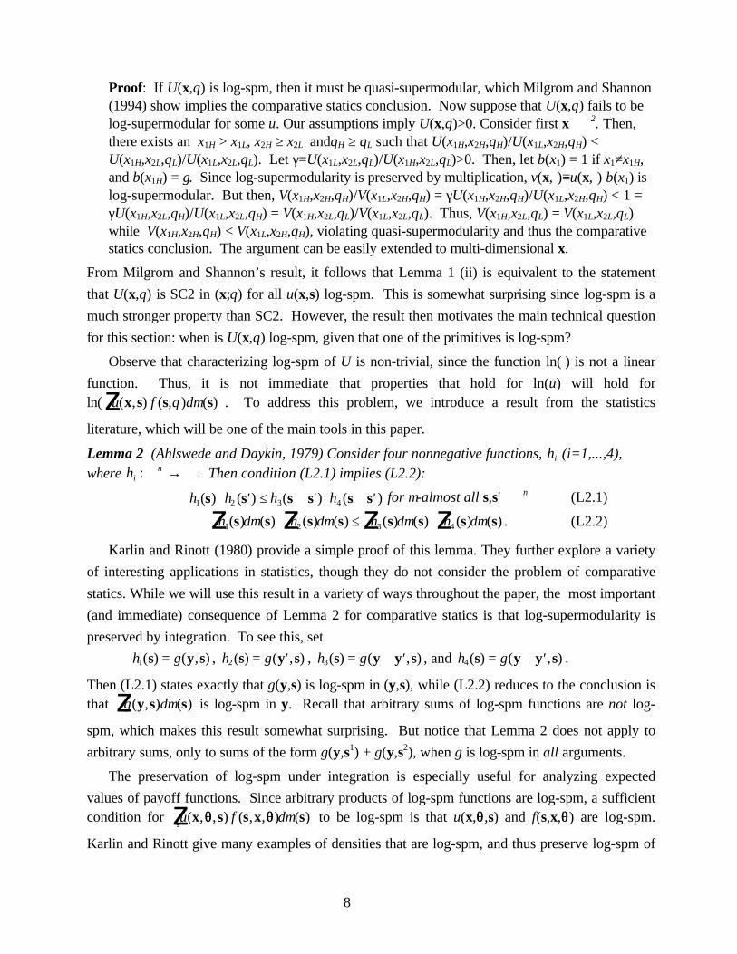
Lemma 2 (Ahlswede and Daykin, 1979) Consider four nonnegative functions, hi (i=1,...,4),where hi : ℜn → ℜ . Then condition (L2.1) implies (L2.2):

h1(s) ⋅ h2 ( ′ s ) ≤ h3(s ∨ ′ s ) ⋅h4 (s ∧ ′ s ) for µ-almost all s,s′∈ℜn (L2.1)

h d h d h d h d1 2 3 4( ) ( ) ( ) ( ) ( ) ( ) ( ) ( )s s s s s s s sz z z z⋅ ≤ ⋅µ µ µ µ . (L2.2)

Karlin and Rinott (1980) provide a simple proof of this lemma. They further explore a variety

of interesting applications in statistics, though they do not consider the problem of comparative

statics. While we will use this result in a variety of ways throughout the paper, the most important

(and immediate) consequence of Lemma 2 for comparative statics is that log-supermodularity is

preserved by integration. To see this, set

h g1( ) ( , )s y s= , h g2( ) ( , )s y s= ′ , h g3( ) ( , )s y y s= ∨ ′ , and h g4( ) ( , )s y y s= ∧ ′ .

Then (L2.1) states exactly that g(y,s) is log-spm in (y,s), while (L2.2) reduces to the conclusion isthat g d( , ) ( )y s sµz is log-spm in y. Recall that arbitrary sums of log-spm functions are not log-

spm, which makes this result somewhat surprising. But notice that Lemma 2 does not apply to

arbitrary sums, only to sums of the form g(y,s1) + g(y,s2), when g is log-spm in all arguments.

The preservation of log-spm under integration is especially useful for analyzing expected

values of payoff functions. Since arbitrary products of log-spm functions are log-spm, a sufficientcondition for u f d( , , ) ( , , ) ( )x s s x s

sθθ θθz µ to be log-spm is that u(x,θθ,s) and f(s,x,θθ) are log-spm.

Karlin and Rinott give many examples of densities that are log-spm, and thus preserve log-spm of

9

a payoff function.15

Despite the fact that log-spm of primitives arises naturally in many economic problems, it is

still somewhat restrictive. Thus, we consider the issue of necessary conditions for log-spm to

hold. Before stating the necessity theorem, we introduce a definition that will allow us to state

concisely theorems about stochastic objective functions throughout the paper. All of the results inthis paper concern problems of the form u f d( , ) ( , ) ( )x s s s

sθθz µ , and in such problems, we wish to

find pairs of hypotheses about u and f which guarantee that a property of U(x,θθ) will hold. We

thus look for what we call a minimal pair of sufficient conditions, defined as follows:

Definition 5 Two hypotheses H-A and H-B are a minimal pair of sufficient conditions (MPSC)for the conclusion C if: (i) Given H-B, H-A is equivalent to C. (ii) Given H-A, H-B is equivalentto C.

This definition introduces a phrase to describe the idea that we are looking for a pair of

sufficient conditions that cannot be weakened without placing further structure on the problem. In

some contexts, H-A will be given (such as an assumption on u), and we will search for the weakest

hypothesis H-B (such as an assumption on f) which preserves the conclusion; in other problems,

the roles of H-A and H-B will be reversed. Though there is no logical requirement that part (ii) of

Definition 5 will hold whenever (i) does, the main results of this paper satisfy all three parts of the

definition. This definition is used to state the following theorem.

Theorem 1 Suppose u:ℜ l × ℜn → ℜ+ and f : ℜn × ℜm → ℜ+ , where n ≥ 2 implies l,m ≥2. Then(A) u(x,s) is log-spm a.e.-µ; and (B) f(s,θθ) is log-spm a.e.-µ; are a MPSC for (C)

u f d( , ) ( , ) ( )x s s ss

θθz µ is log-spm in (x,θθ).

Remark Theorem 1 requires that x has at least two components (l=2) if n≥2, so that the class ofu’s is sufficiently rich to make log-supermodularity of f in s a necessary condition. However,even in cases where n≥2 and l=1, log-supermodularity of f in (si,θ) is necessary for theconclusion (T1-C) to hold whenever (T1-A) does.

Theorem 1, which is proved formally in the appendix, states that, not only do (A) and (B) imply

the conclusion, but neither restriction can be relaxed without placing additional restrictions on the

other primitive. While in Theorem 1, the conditions on u and f are the same (log-spm), in our

subsequent theorems we will pair different conditions, such as single crossing and log-spm, for

different conclusions. Together with Lemma 1, this result can be used to provide necessary and

sufficient conditions for comparative statics conclusions. Before proceeding to that result, we

develop the proof of Theorem 1, and identify its limitations.

The proof of Theorem 1 can be understood with reference to the stochastic dominance

15 For example, symmetric, positively correlated normal or absolute normal random vectors have a log-supermodular density (but arbitrary positively correlated normal random vectors do not; Karlin and Rinott (1980)give restrictions on the covariance matrix which suffice); and multivariate logistic, F, and gamma distributions havelog-supermodular densities.

10

literature, and more generally Athey (1995), which exploits a “convex cone” approach to

characterizing properties of stochastic objective functions. Athey (1995) shows that in stochastic

problems, if one wishes to establishes that a property P holds for U(x,θ) for all u in a given class U,

it is often necessary and sufficient to check that P holds for all u in the set of extreme points of U.

The extreme points can be thought of as test functions; for example, when U is the set of

nondecreasing functions, the set of test functions is the set of indicator functions for sets 1A(s) that

are nondecreasing in s. Athey (1995) shows that this approach is the right one when P is a

property preserved by convex combinations, unlike log-supermodularity.

Despite the fact that the “convex cone” approach does not apply directly here, an analogous

intuition can still be developed. Consider the hypothesis that the set of “test functions” for log-supermodular functions is the set of indicator functions of the form 1 xBε ( ) , where Bε (x ) is defined

to be a cube of length ε around the point x. This set of test functions will certainly yield T1-B as a

necessary condition for T1-C: only if f(s,θθ) is log-supermodular almost everywhere-µ will1 s s sxs B f dε µ( ) ( ) ( , ) ( )θθz be log-supermodular in (x;θθ). But, it remains to establish that this set of

test functions satisfies T1-A. The following lemma can be used:

Lemma 3 The indicator function 1A(τ)(s) is log-spm in (s,τ) if and only if A(τ) is nondecreasing(strong set order). Further, 1A(s) is log-spm in s if and only if A is a sublattice.

Proof: Simply verify the inequalities and check the definitions. 1A(τ)(x) is log-spm in (s,τ) ifand only if: 1 s s 1 s s 1 s 1 s

A A A AH L H L( ) ( ) ( ) ( )( ) ( ) ( ) ( )τ τ τ τ∨ ′ ⋅ ∧ ′ ≥ ⋅ ′ . The definitions imply that if the

right-hand side equals one, the left-hand side must equal one as well. Likewise, 1A(s) is log-spm in s if and only if: 1 s s 1 s s 1 s 1 sA A A A( ) ( ) ( ) ( )∨ ′ ⋅ ∧ ′ ≥ ⋅ ′ . Again, this corresponds exactly tothe definition.

It is straightforward to verify that sets of the form ×i i ia b[ , ] are sublattices, as desired. Further,

such sets are nondecreasing (strong set order) in each endpoint. Lemma 3 leads to an important

role for the strong set order and sublattices in the analysis of stochastic optimization problems.

Lemma 3 will also be useful in many applications, for example (as the pricing game of Section 3.2)

when the choice variables or parameters affect the domain of integration.

The analogy to the “test functions” approach, and thus the proof of Theorem 1, can be made

complete with the following lemma.

Lemma 4 (Test functions for log-spm problems) Define the setT(β)≡{u:∃ x and 0<ε<β such that u(x,s)=1 sxBε ( ) ( ) }.

Then U(x,θθ)= u f d( , ) ( , ) ( )x s s ss

θθz µ is log-spm in (x,θθ) whenever u(x,s) is log-spm a.e.-µ., if and

only if, for some β>0, U(x,θθ) is log-spm whenever u∈T(β).

Lemma 4 establishes the limits of Theorem 1 by identifying which additional regularity properties

of u will change the conclusion of Theorem 1. For example, the elements of T(β) are clearly not

monotonic, and thus Theorem 1 does not hold under the additional assumption that u is

nondecreasing. In contrast, we can clearly approximate the elements of T(β) with smooth

11

functions, so smoothness restrictions will not alter the conclusion of Theorem 1.

Together, Lemma 1, Theorem 1, and Lemma 3 can be used to establish the first main

comparative statics theorem of the paper, which states necessary and sufficient conditions for

comparative statics in problems with log-supermodular payoff functions.

Corollary 1.1 (Comparative Statics with Log-Supermodular Primitives) Consider functionsw:ℜl ×ℜm×ℜn→ℜ+, f:ℜn×ℜm→ℜ+, A

j:ℜ→2 ℜn

, j=1,..,J. Let A( ) ( ),..,ττ = ∩ =j Jj

jA1 τ . Let x*(θθ,ττ,B)

= argmaxx∈BW(x,θθ,ττ)≡ w f d( , , ) ( ; ) ( )( )

x s s ss A

θθ θθττ

µ∈z .

(1) (Necessary and sufficient conditions) Suppose A(ττ) is a sublattice, θθ∈ℜ, and l≥2 if n≥2.Then x*(θθ,ττ,B) is nondecreasing in θθ for all w log-spm, if and only if f is log-spm a.e.-µ on A(ττ).(2) (General sufficiency) x*(θθ,ττ,B) is nondecreasing in (θθ,ττ,B) if w and f are log-supermodular,and, for each j, A j (τ j ) is nondecreasing (strong set order) in τ j .

Proof: (1) Necessity: by Lemma 1, the comparative statics conclusion is equivalent to log-supermodularity of W in (x,θθ). Then we can apply Theorem 1. Sufficiency follows by: (2)Since products of log-spm functions are log-spm, the functionw f

A A JJ

( , , ) ( ; ) ( ) ( )( ) ( )

x s s 1 s 1 sθθ θθ ⋅ ⋅⋅ ⋅11τ τ

is log-spm in (s,x,θθ,ττ) by Lemma 3.

Note that the objective function analyzed in Corollary 1.1 is not a conditional expectation, since

we have not divided by the probability that s∈A(ττ). Further, observe that (1) is not stated in terms

of a minimal pair of sufficient conditions. The reason is that Lemma 1 only yields necessary

conditions for comparative statics if we quantify over all payoffs u(x,s), where u contains the

choice variables. In general, log-spm is sufficient, but not necessary, for MCSa.

While Corollary 1.1 is straightforward given the building blocks outlined above, it shows that

problems a structure commonly encountered in economic theory can be analyzed by checking a

few simple conditions. The following applications illustrate the theorem.

3.1. Applications to Investment Under Uncertainty

An immediate implication of Corollary 1.1 is that a ratio orderings over distributions,

commonly used in the literature on investment under uncertainty, can be easily compared: loosely,

integrating a function makes it more likely to be log-spm. If a distribution satisfies the MLR order

(that is, the density is log-spm), then the corresponding cumulative distribution function F(s;θ) will

also be log-spm,16 which can be shown to be stronger than First Order Stochastic Dominance.

This will in turn imply that F s dsa

( ; )θ−∞z is log-spm, which is stronger than Second Order

Stochastic Dominance if θ does not change the mean of s.

More generally, we can consider any ratio ordering which specifies that g(s)/h(s) is

nondecreasing in s for g,h>0. The easiest way to fit this into our framework is to define u(x,s) on

16 See Eeckhoudt and Gollier (1995) who term this the monotone probability ratio (MPR) order, and show that anMPR shift is sufficient for a risk-averse investor to increase his portfolio allocation.

12

{0,1}×ℜ, and let u(x,s) = g(s) if x=1, and let u(x,s) = h(s) if x=0. Then, if f(s;θ) is log-spm and

g(s)/h(s) is nondecreasing in s, E[g(s)|θ]/E[h(s)|θ] must be nondecreasing in θ. Further, Theorem

1 shows that log-spm of f is the weakest condition which preserves every ratio ordering.

An example from the economics of uncertainty is the Arrow-Pratt coefficient of risk aversion,

R(w;u)≡ −u′′(w)/u′(w). Suppose that an agent has decreasing absolute risk aversion (DARA) and

faces a risk s with distribution F(s;θ). Let U(w;θ) = ∫u(w+s)f(s;θ)ds, and observe that u′(w+s) is

log-spm if and only if R(w;u) is nonincreasing in w (DARA). Theorem 1 then implies that in

response to an MLR shift in the risky asset s, the agent will be less risk averse when considering a

new, independent risk. But, observe that the fact that w and s enter u additively precludes the test

functions of Lemma 4, so necessity cannot be obtained using Theorem 1 for risk averse agents.

A further consequence of Theorem 1 is that orderings over risk aversion and related properties

are preserved with respect to background risks. Let U(w) = ∫u(w+s)f(s)ds. If R(w;u) is decreasing,

it then follows from Theorem 1 that U′(w+t) will be decreasing as well, implying that R(w;U) is

decreasing. Similar analyses apply to other ratio orderings, such as Kimball’s (1990) decreasing

prudence condition,17 where prudence is defined by −u′′′(w)/u′′(w).18 More generally, we can

consider orderings of utilities over risk aversion (not just those induced by a shift in wealth). Let θparameterize the agent’s risk aversion directly, and let U(w;θ) = ∫u(w+s;θ)f(s)ds. Then if

R(w;u(⋅;θ)) is nonincreasing in w and θ, U inherits these properties, so that R(w;U(⋅;θ)) isnonincreasing in θ and w. Other ratio orderings can be similarly analyzed.

Finally, Theorem 1 allows us to consider more general background risks, those which might be

statistically dependent on the risk of primary interest. Let z be the “primary” risk, and let s be a

vector of assets in which the agent also has a position, represented by the vector of positive

portfolio weights αα. The agent’s utility is given by U(z,θ) = ∫u(z+αα⋅s;θ)f(s|z)ds. Suppose that the

risks are affiliated, that is, f(s,z) is log-spm. But, applying the multivariate Theorem 1, the agent’s

risk aversion with respect to z (that is, R(z;U,θ)) will be nonincreasing in θ, if u satisfies DARA

and θ decreases risk aversion. An alternative, but distinct sufficient condition requires that the

conditional density of y=αα⋅s given z, g(y|z), is log-spm.

This analysis thus provides several extensions to the existing literature. Jewitt (1987) showed

that the “more risk averse” ordering is preserved by a MLR shift in the distribution, while Pratt

(1988) established that risk aversion orderings are preserved by expectations. Eeckhoudt, Gollier,

and Schlesinger (1996) provide additional conditions on distributions under which a FOSD shift in

a background risk decreases risk aversion for a DARA investor. The above analysis generalizes

17 Kimball (1990) shows that agents who are more prudent will engage in a greater amount of “precautionary

18 It is interesting to observe that since a smooth function g(x+y) is supermodular if and only if it is convex, theseresults can also be proved using the fact that log-convexity is preserved under expectations (Marshall and Olkin,1979); but, the correspondence between convexity and supermodularity breaks down with more than two variables.

13

these results by showing that all of the results extend to other ratio orderings, such as prudence,

and further risk aversion orderings are preserved by affiliated background risks for DARA

investors.

3.2. Log-Supermodular Games of Incomplete Information

This section establishes sufficient conditions for a class of games of incomplete information to

have a PSNE in nondecreasing strategies. Consider a game of incomplete information between

many players, each of whom has private information about her own type, ti, and chooses a strategy

χi(ti). Vives (1990) observed that the theory of supermodular games (Topkis, 1979) can be

applied to games of incomplete information. He showed that if each player’s payoff vi(x) is

supermodular in the realizations of actions x, the game has strategic complementarities in

strategies χj(tj) (that is, a pointwise increase in an opponent’s strategy leads to a pointwise increase

in a player’s best response). This in turn implies that a PSNE exists.

In contrast, if we consider the same problem but assume that vi(x) is log-spm, it is no longer

true that the game has strategic complementarities in stategies in the sense just described.

However, we can instead take a different approach: Athey (1997) shows that a PSNE exists in

games of incomplete information where an individual player’s strategy is nondecreasing in her own

type (i.e. χi(tiH)≥χi(ti

L)), whenever all of her opponents use nondecreasing strategies.

Formally, suppose that h(t) is the joint density over types. Let player i’s utility be given by

vi(x,t) (so that opponents’ types might influence payoffs both directly and indirectly, through the

opponents’ choices of actions). Thus, a player’s payoff given a realization of types can be written

ui(xi,t)≡vi(xi,χχ−i(t−i),t). Taking the expectation over opponent types yields the following expressionfor expected payoffs: U x t u x h t di i i i i i i i i

i( , ) ( , ) ( )≡ − −

−z t t ts

. The following result gives sufficient

conditions for a player’s best response to nondecreasing strategies to be nondecreasing.

Proposition 1 Let h:ℜn→ℜ+, where h(t) is a probability density. Assume that h has a fixed,convex support. For i=1,..,n, let hi(t−i|ti) be the conditional density of t−i given ti, and definepayoffs as above. Then (i) for all i, χi(ti) = arg max ( , )x i ii

U x t is nondecreasing (strong set order)

in ti for all χj(tj) nondecreasing for j≠i, and vi log-spm, if and only if (ii) h(t) is log-spm almosteverywhere-Lebesgue on the support of t.

Proof: Sufficiency follows from Lemma 2 and Milgrom and Shannon (1994). Following theproof of Theorem 1, it is possible to show that Ui(xi,ti) is log-supermodular for all ui(xi,t) log-supermodular, only if, for all t t− −>i

Hi

L and all t tiH

iL> , h t h t h t h ti i

HiH

i iL

iL

i iL

iH

i iH

iL( | ) ( | ) ( | ) ( | )t t t t− − − −≥ .

But, since for a positive function, log-spm can be checked pointwise, this condition holds forall i if and only if h is log-spm. Apply Lemma 1.

Spulber (1995) recently analyzed how asymmetric information about a firms’ cost parameters

alters the results of a Bertrand pricing model, showing that there exists an equilibrium where

prices are increasing in costs, and further firms price above marginal cost and have positive

expected profits. Spulber’s model assumes that costs are independently and identically distributed,

14

and that values are private; Proposition 1 easily generalizes his result to asymmetric, affiliated

signals, and to imperfect substitutes. Let vi(x,t) = (xi−ti)⋅Di(x), where x is the vector of prices, t is

the vector of marginal costs, and Di(x) gives demand to firm i when prices are x.

By Theorem 1, the expected demand function is log-spm if the signals are affiliated, each

opponent uses a nondecreasing strategy, and Di(x) is log-spm. The interpretation of the latter

condition is that the elasticity of demand is a non-increasing function of the other firms’ prices.

Demand functions which satisfy these criteria include logit, CES, transcendental logarithmic, and a

set of linear demand functions (see Milgrom and Roberts (1990b) and Topkis (1979)). Further,

when the goods are perfect substitutes, expected demand is also log-spm. To see this, note that

when each opponent uses a nondecreasing strategy, expected demand is given by

D x t t h t dt x t xn n

1 1 2 2 1 1 12 2 1 11

( ) ( ) ( ) ( )( ) ( )1 1 t tt χ χ> > − −⋅ ⋅

−z

and the set t t xj j j: ( )χ > 1l q is nondecreasing (strong set order) in x1 when χj is nondecreasing.

Then, by Lemma 3 and Corollary 2.1, expected demand must be log-spm when the density is.

Thus, a PSNE exists in nondecreasing pricing strategies whenever marginal cost parameters

are affiliated and demand is log-spm and continuous, or in the case of perfect substitutes.

3.3. Conditional Stochastic Monotonicity and Comparative Statics

Corollary 2.1 applies to stochastic problems where the domain of integration is restricted, but

not to conditional expectations. Conditional expectations of multivariate payoff functions arise in

a number of economic applications, such as the “mineral rights auction” (Milgrom and Weber,

1982). This section studies comparative statics when the agent’s objective takes the form

U(x,θ|A(τ))≡ u x f A dA

( , ) ( , ( )) ( )s s sθ τ µz = u xf

f dd

AA

( , )( , )

( , ) ( )( )

( )( )

ss

s ss

θθ µ

µτ

τ zz .

The comparative statics condition of interest in this problem is

x*(θ,τ,B)=argmaxx∈B U(x,θ|A(τ)) is nondecreasing in (θ,τ). (MCSb)

Before proceeding, we need another definition: we say that u(x,s) satisfies nondecreasing

differences in (x;s) if u(xH,s)−u(xL,s) is nondecreasing in s for all xH≥xL. In terms of the vector s,

this assumption is clearly weaker than log-supermodularity of u in s, since no assumptions on the

interactions between the components of s are imposed; however, nondecreasing differences is

neither weaker nor stronger than log-spm, unless u satisfies additional monotonicity restrictions.

Our focus on supermodularity of U(x,θ|A(τ)) in the study of comparative statics in problems

for this class of payoff functions is motivated by the following result (Athey, 1995), which is

analogous to Lemma 1: for a given τ, U(x,θ|A(τ)) satisfies SC2 in (x,θ) for all u which satisfy

nondecreasing differences in (x;s), if and only if U(x,θ|A(τ)) in (x;θ) is supermodular for all u which

satisfy nondecreasing differences in (x;s).

Of course, U(x,θ|A(τ)) is supermodular in (x,θ) if and only if U(xH,θ|A(τ)) −U(xL,θ|A(τ)) is

15

nondecreasing in θ for all xH>xL, and thus the problem reduces to checking thatG A g f A d

A( ( )) ( ) ( , | ( )) ( )θ τ θ τ µ≡ z s s s is nondecreasing in θ and τ for all g nondecreasing. The

following theorem applies to this problem:

Theorem 2 Consider f n:ℜ → ℜ++

1 . Then (A) g S: → ℜ is nondecreasing a.e.-µ; and (B) f (s;θ)

is log-spm a.e.-µ; are a MPSC for (C) G(θ|A(τ)) is nondecreasing in τ and θ for all A(τ)nondecreasing in the strong set order.

Theorem 2 is a generalization of a result which has received attention in both statistics and

economics (Sarkar (1968), Whitt (1982), Milgrom and Weber (1982)).19 To see the proof of

sufficiency using Lemma 2, consider the case where g is nonnegative. Consider τH > τL and θH > θL,

and define the following functions:

h g fA LL1( ) ( ) ( ) ( ; )( )s s 1 s ss= ⋅ ⋅∈ τ θ , h fA HH2( ) ( ) ( ; )( )s 1 s ss= ⋅∈ τ θ ,

h g fA HH3( ) ( ) ( ) ( ; )( )s s 1 s ss= ⋅ ⋅∈ τ θ , and h fA LL4( ) ( ) ( ; )( )s 1 s ss= ⋅∈ τ θ .

It is straightforward to verify under our assumptions that h h h h1 2 3 4( ) ( ) ( ) ( )s s s s s s⋅ ′ ≤ ∨ ′ ⋅ ∧ ′ (using

Lemma 3 and the fact that log-spm is preserved by multiplication); thus, Lemma 2 gives us

g f d f d g f d f dA L HA A H LAL H H L

( ) ( ; ) ( ) ( ; ) ( ) ( ) ( ; ) ( ) ( ; ) ( )( ) ( ) ( ) ( )

s s s s s s s s s ss s s s∈ ∈ ∈ ∈z z z z⋅ ≤ ⋅

τ τ τ τθ µ θ µ θ µ θ µ .

Rearranging the inequalities gives the desired ranking, G(θL|AL)≤G(θH|AH).

The stochastic monotonicity results can then be exploited to derive necessary and sufficient

conditions for comparative statics conclusion in problems of the U(x,θ,τ). In particular, we have

the following corollary:

Corollary 2.1 (Comparative Statics with Conditional Expectations) Consider any A(τ), andsuppose F(s,θ) is a probability distribution. Then MCSb holds for all u which satisfynondecreasing differences in (s;θ), if and only if f(s,θ) is log-supermodular a.e.-µ.

Finally, we examine the limits of the necessity part of Theorem 2. The counter-examples we

construct require us to condition on an arbitrary sublattice. If the economic problem places

additional structure on the set A, log-spm is no longer necessary. Consider a particular case which

arises very commonly in applications (such as auctions): assume there is a single random variable,

and let A(τ)=11{s<τ} . In this case, log-supermodularity of the density is not necessary for monotone

comparative statics predictions, but instead, we require the distribution to be log-spm.

Corollary 2.2 Consider a probability distribution F(s;θ), s∈ℜ, and restrict attention toA(τ)=11{s<τ}. Then MCSb holds for all u(x,s) supermodular, if and only if F(s;θ) is log-spm.

4. Comparative Statics with Single-Crossing Payoffs and Densities

This section studies single crossing properties in problems where there is a single random

19 Sarkar (1968) establishes sufficiency, and Whitt (1982) studies conditions under which G(θ|A) is increasing in θfor all sublattices A; Milgrom and Weber (1982) study conditions under which G(θ|A) is increasing in θ and also ina limited class of shifts in A.

16

variable. Multivariate generalizations of the results are sufficiently restrictive that they are not

considered here. However, many problems in the theory of investment under uncertainty,

auctions, and signaling games can be fruitfully analyzed with a single random variable.

Problems of the form U(x,θ)≡ u x s f s d s( , ) ( ; ) ( )θ µz , where all variables are real numbers, are a

special case of those considered in Section 3. This section seeks to relax the assumption that both

primitives are log-spm. In particular, we consider the weaker assumption that u(x,s) satisfies SC2

in (x;s). Problems which fit into this framework include mineral rights auction games and

investment under uncertainty problems. The problem of interest is

x*(θ,B)=argmaxx∈B U(x,θ)≡ u x s f s d s( , ) ( ; ) ( )θ µz is nondecreasing in θ. (MCSc)

Our results from Section 3 give some initial insight into this problem: they imply that a

necessary condition for (MCSc) to hold for all u which are SC2 is that f(s,θ) is log-spm. a.e.-µ.

To see this, observe that since SC2 is weaker than log-spm, if (MCSc) holds for all u(x,s) which

satisfy SC2, then (MCSc) must hold for all u(x,s) log-spm. By Corollary 1.1, this implies that

f(s,θ) is log-spm a.e.-µ. However, since SC2 is weaker than log-spm, our results from Section 3

do not establish that u SC2 and f log-spm are sufficient for (MCSc). To analyze this question, it

will be useful to transform the problem by taking a the first difference with respect to x, since

U(x,θ) and u(x,s) satisfy SC2 if and only if, for all xH>xL, U(xH,θ)−U(xL,θ) and u(xH,s)−u(xL,s)satisfy SC1. Thus, we study conditions under which G(θ)≡ g s k s d s( ) ( , ) ( )θ µz satisfies SC1 in θ.

Section 4 proceeds as follows. Section 4.1 analyzes SC1 of G(θ) and applications which are

most easily analyzed from that perspective, such as the portfolio problem. This section develops

the main technical ideas of Section 4. Section 4.2 considers (MSCc) directly, and provides

additional applications. Section 4.3 considers comparative statics using the Spence-Mirlees single

crossing property (SC3). The main results are summarized in Table 1 in the conclusion.

4.1. SC1 in Stochastic Problems

The main result of this section finds the minimal sufficient conditions for our single crossing

conclusion.

Theorem 3 Let K(s;θ) be a distribution. (A) g(s) satisfies SC1 in (s) a.e.-µ20; and (B) K(s;θ)satisfies MLR; are a MPSC for (C) G(θ)= g s dK s( ) ( ; )z θ satisfies SC1 in θ.

Extensions to Theorem 3:21 Theorem 3 also holds if: (i) there exists k and µ such that

K(s;θ)= k t d ts

( , ) ( )θ µ−∞z for all θ, in which case (B) is equivalent to k is log-spm a.e.-µ;

(ii) g depends on θ directly, under the additional restrictions that g is piecewise continuous in θ

20 We will say that g(s) satisfies SC1 almost everywhere-µ (a.e.-µ) if conditions (a) and (b) of the definition of SC1hold for almost all (w.r.t. the product measure on ℜ2 induced by µ) (sH,sL) pairs in ℜ2

such that sH>sL.21 A version of this theorem which gives minimal sufficient conditions for strict single crossing is provided inAthey (1996).

17

and g is nondecreasing in θ (see also Theorem 5 below for another sufficient condition);(iii) g(s) satisfies only WSC1, provided supp[K(s;θ)] is constant in θ.

The theory of the preservation of single crossing properties under uncertainty has a long

history in the statistics literature. Karlin and Rubin (1956) establish sufficiency, and Karlin (1968)

(pp. 233-237) analyzes necessary conditions,22 under the absolute continuity assumption of

Extension (i) and some additional regularity conditions (including the assumption that Θ has at

least three points).23 When K is a probability distribution, the ex ante absolute continuity

assumption may be undesirable; however, if k represents a utility function, it is the right

assumption.

We will outline the proof in the text. The sufficiency proof is surprisingly simple, and our

applications will show that it can be easily modified to produce extensions of Theorem 3. In

addition, in this section (as we did in Lemma 4 and Section 3.3), we identify the smallest class of

functions which is required to generate the counter-examples used to prove necessity; this will be

useful for analyzing the tradeoffs between alternative assumptions on primitives. In Section 4.1.1,

we illustrate in applications how additional commonly encountered restrictions on g or k can be

used to relax (T3-A) and (T3-B).

Consider first sufficiency. Suppose for simplicity that k(s,θ)>0. Define l(s)= k ( s;θ H ) k( s;θL ) ,

which (4.1-B) guarantees is nondecreasing. Notice first that, for a given θH >θ L,

g s k s d sH( ) ( ; ) ( )z θ µ = g s k s k s k s d sH L L( ) ( ; ) ( ; ) ( ; ) ( )z θ θ θ µb g . Let s0 be a point where g crosses

zero. Then:g s k s d s g s l s k s d s

g s l s k s d s g s l s k s d s

l s g s k s d s l s g s k s d s l s g s k s d s

H L

sL s L

sL s L L

( ) ( ; ) ( ) ( ) ( ) ( ; ) ( )

( ) ( ) ( ; ) ( ) ( ) ( ) ( ; ) ( )

( ) ( ) ( ; ) ( ) ( ) ( ) ( ; ) ( ) ( ) ( ) ( ; ) ( )

z zz z

z z z

=

= − +

≥ − + =−∞

∞

−∞

∞

θ µ θ µ

θ µ θ µ

θ µ θ µ θ µ

0

0

0

00 0 0

(4.1)

The second equality holds because g satisfies SC1, while the inequality follows since monotonicity

of l implies the following condition, which is necessary (4.1) to hold:

l(s) ≤ l(s0) for s<s0, while l(s) ≥ l(s0) for s>s0. (4.2)

(4.2) requires that the likelihood ratio l(s) satisfies WSC1(s0). (In Section 4.1.1 below, we will

show how fixing the crossing point can allow us to exploit (4.2) as a sufficient condition). If, inaddition, l(s0)≤1, then g s k s d sH( ) ( ; ) ( )z θ µ ≤0 implies g s k s d sL( ) ( ; ) ( )z θ µ ≤ g s k s d sH( ) ( ; ) ( )z θ µ ;

this case arises when k(s;θ) is a probability distribution (not a density). In that case, if l(s) is

nondecreasing, it must always be less than 1, which is its value at the highest s.

The necessity parts of this theorem can be proved by constructing counterexamples, which

22 I am grateful to an anonymous referee who directed me to this theorem.23 The necessity proof provided in Karlin (1968) is designed to solve a much more general problem (about thepreservation of an arbitrary number of sign changes, and thus it requires additional regularity assumptions and acomplicated construction.

18

place all of the weight on the failures. Thus, the proof of Theorem 3 makes use of the following:

Lemma 5 (Test functions for single crossing problems) Define the following sets:G(β)≡ {g: ∃a,b>0, β>ε,δ>0, and sL<sH s.t. g(s)=−a for s∈(sL−ε,sL+ε) and

g(s)=b for s∈(sH−ε,sH+ε), |g|<δ elsewhere, and g satisfies SC1}K(β)≡ {k: ∃a>0, β>ε>0 and s0 s.t. k(s)=a for s∈(s0−ε,s0+ε), and k=0 elsewhere}.

Then Theorem 3 holds if, for any β>0, (4.1-A) is replaced with (4.1A’) g(s)∈G(β); Theorem 3 alsoholds if (4.1-B) is replaced with (4.1B’) k(s,θ)∈K(β).

As in Theorem 1, placing smoothness assumptions on g will not change the conclusion of

Theorem 3, but monotonicity or curvature assumptions will. If monotonicity of one of the

primitives is assumed (for example, if k is a probability distribution, not a density), then the

necessity parts of the theorem break down, as shown in Section 4.2.1.

Now consider how the counter-examples are used. If g fails (T3-A), then there is sL < sH such

that g(sL)≥0, but g(sH)<0, on sets SL and SH of positive measure µ. But then, k(s;θ) can be defined

so that k(s;θH) places all of the weight on high points sH, while k(s;θL) places all of the weight on

the low points sL. This function is log-spm, but G(θ) fails SC1 since g does. If k fails (T3-B), then

there exist two sets of positive measure, SH and SL, such that increasing θ places more weight on SL

relative to SH. Then we can construct a g(s) that is negative on SL, positive on SH, and close to

zero everywhere else.

However, the proof of necessity of (T3-B) involves some additional work. Theorem 3 does

not place ex ante restrictions on how supp[K(s;θ)] moves with θ. The restrictions implied when

(T3-C) holds whenever (T3-A) does are summarized in the following Lemma.

Lemma 6 If g s dK s( ) ( ; )z θ satisfies SC1 in θ whenever g satisfies SC1 in s, (i) for all θH>θL,

K(s;θH) is absolutely continuous with respect to K(s;θL) on (infssupp[K(s;θH)], supssupp[K(s;θL)]),and (ii) supp[K(s;θ)] is nondecreasing in the strong set order.

The following applications show how additional structure present in particular problems can be

exploited; they also generalize the result to allow k to cross zero.

4.1.1. Extensions and Applications to Investment Problems

This section uses Theorem 3 to analyze two classic problems, the portfolio investment problem

and the decision problem of a risk averse firm. We develop extensions to Theorem 3 which allow

us to generalize several comparative statics results previously established only for special

functional forms.

Consider first the standard portfolio problem, where an agent with initial wealth w invests x ina risky asset s, and receives payoffs u w x r sx(( ) )− + . The first order conditions are given by

′ − + −z u w x r sx s r f s ds(( ) )( ) ( , )θ . (4.3)

Notice that s−r satisfies single crossing, and further, the crossing point is fixed at s0=r for all utility

19

functions. This section identifies how (T3-B) can be weakened using this additional structure. We

begin with an additional definition.

Definition 5 We will say that k(s;θ) satisfies weak single crossing of ratios about s0, denoted

WSCR(s0) if (i) $( ) lim ( , ) ( , )l s k s k ss sH L

0 0= → θ θ exists, (ii) supp[K(s,θ)] is nondecreasing in the

strong set order, (iii) either k≥0 or k satisfies WSC1(s0), and (iv) k(s,θH)/k(s,θL) − $( )l s0 satisfies

WSC1(s0) for s where k(s;θL)⋅k(s;θH)>0.

While the WSCR(s0) condition may appear unfamiliar, it is potentially quite useful. In

particular, it allows that the function k could itself cross zero, though we will not exploit that fact

until the next subsection. To start, we observe that if k is nonnegative, then k(s,θ) satisfies

WSCR(s0) for all s0 if and only if k is log-spm. Further, WSCR(s0) can be satisfied if k(s,θH) and

k(s,θL) cross exactly once, at s0. If k is a probability distribution and the mean of s does not change

with θ, it is known that such a single crossing property of the distribution implies that θ indexes k

according to second order stochastic dominance.

To see how the weak single crossing property of ratios can be used to establish single crossing

conclusions, recall that the inequality in (4.1) holds whenever (4.2) holds. However, for a fixed s0

and for k≥0, (4.2) is equivalent to WSCR(s0). Thus, if we know that g satisfies WSC1(s0), (4.1)

will hold whenever k(s,θ) satisfies WSCR(s0).

Theorem 4: Suppose that supp(K) is constant in θ and k is nonnegative. Then (A) g(s) satisfiesWSC1(s0) in (s) a.e.-µ, and (B) k(s;θ) satisfies WSCR(s0) a.e.-µ, are a MPSC for (C)G(θ)= g s k s d s( ) ( , ) ( )θ µz satisfies SC1 in θ:

Consider how this result relates to Theorem 3. If we relax (T3-A) to allow for WSC1 around

any point, we must strengthen (T3-B) so that k is restricted to be log-spm. Consider an

application of this result. In the portfolio problem, we can apply Theorem 4 to (4.3), letting g=s−r

and k=u′⋅f. Then the optimal portfolio allocation x*(θ,B,r) is nondecreasing in θ whenever f(s,θ)

satisfies WSCR(r). But, if we desire a comparative statics result for all r, log-supermodularity of f

will be required. In many problems the relevant range for the risk-free rate may be smaller than the

support of the risk-free asset, and thus Theorem 4 has content.

The portfolio problem has been widely studied. However, far fewer results have been obtained

for more general investment problems, where potentially risk-averse firms invest in a risky projects

π(x,s), or make pricing or quantity decisions under uncertainty about demand. Suppose that anagent’s objective is as follows: maxx∈B u x s f s d s( ( , ), ) ( , ) ( )π θ θ µz , and the solution set is denoted

x*(θ,B). Thus, π represents a general return function which depends on the investment amount, x,

and the state of the world, s. The agent’s utility depends on the returns to the project as well as

some exogenous parameter θ, which might represent initial wealth or some other factor relating to

risk aversion. Notice that in this problem, the crossing point of π is not automatically determined

as in the portfolio problem.

20

When this objective function is differentiable, it suffices to check that the marginal returns to x,denoted u x s x s f s d sx1( ( , ), ) ( , ) ( , ) ( )π θ π θ µz , satisfy SC1. However, we might also wish to allow

for the possibility that the agent faces discrete choices between investments, or that the function πis endogenously determined (so that regularity properties of π cannot be assumed). To analyze

this problem, we introduce another extension to Theorem 3, as follows:

Theorem 5 Suppose that (i) supp(K) is constant in θ, (ii) g(s,θ) satisfies WSCR(s0) a.e.-µ for allθ; and (iii) k(s,θ) is log-spm a.e.-µ. Then G(θ)= g s k s d s( , ) ( , ) ( )θ θ µz satisfies SC1 in θ.

Proof: Consider the case where g crosses 0 (otherwise, the expectation is always non-negative) and g=0 only at s=s0, and k>0; the other cases can be handled in a manner similar tothe proof of Theorem 3. Then, we extend (4.1) as follows:

g s k s d sg s k s

g s k sg s k s d s g s k s d s

g s k s

g s k sg s k s d s

H H

s s

H H

L L

Ls

L Ls L

s s

H H

L LL L

( ; ) ( ; ) ( )

lim( ; ) ( ; )

( ; ) ( ; )( ; ) ( ; ) ( ) ( ; ) ( ; ) ( )

lim( ; ) ( ; )

( ; ) ( ; )( ; ) ( ; ) ( )

θ θ µθ θθ θ

θ θ µ θ θ µ

θ θθ θ

θ θ µ

zz z

z≥ − +

=

→ −∞

∞

→

0

0

0

0

The inequality follows, as in Theorem 3, because g satisfies WSC1(s0), and g⋅k satisfiesWSCR(s0) since g and k do.

Proposition 2 Consider the problem maxx ∈B

u x s f s d s( ( , ), ) ( , ) ( )π θ θ µz . Assume that u(y,θ) is

increasing and differentiable24 in y and π(x,s) is nondecreasing in s. Then:

(A) π(x,s) satisfies SC2 in (x;s) a.e.-µ, and (B) u y f s1( , ) ( , )θ θ is log-spm. in (s,y,θ) a.e.-µ,25 are a

MPSC for the conclusion (C) x*(θ,B) is nondecreasing in θ.

Proof: (A) and (B) imply (C): If π is differentiable in x and B is a convex set, we can analyzewhether u x s x s f s d sx1( ( , ), ) ( , ) ( , ) ( )π θ π θ µz satisfies SC1. We can let g=πx, and let k=u1⋅f, and

apply Theorem 3. Now consider the investor’s choice between two values of x, x H > x L .Then, let g(s,θ) = u(π(xH,s),θ)−u(π(xL,s),θ), and let k(s;θ) = f(s;θ). First, observe that SC2 ispreserved under monotone transformations, so that if u is nondecreasing in its first argument,then by (A), u(π(x,s),θ) must satisfy SC2 in (x;s), and g(s,θ) satisfies SC1 in s. Now, considerconditions under which g(s,θ) satisfies WSCR(s0). Let s0 be the crossing point of πx. First

restrict attention to s≥s0, where π(xH,s) ≥π(xL,s). Define h(a,b,θ)= u y dyy a

b1( , )θ

=z , and note that

h is log-spm in (a,b,θ) for all a<b, by Corollary 2.1 and (B). This in turn implies thatg(s,θ)=h(π(xL,s),π(xH,s),θ) is log-spm in (s,θ) on s≥s0 since π is nondecreasing in s, and thusg( s;θH ) g(s ;θL ) is nondecreasing in s on s≥s0. On the other hand, if s<s0, π(xH,s)≤π(xL,s), andg(s,θ)= −h(π(xH,s),π(xL,s),θ). Then, g( s;θH ) g(s ;θL ) is nondecreasing in s on s<s0 since h islog-spm, and WSCR(s0) holds. Then apply Theorem 5. Necessity follows by Theorem 3 forthe case where π is differentiable; the proof is omitted for the more general case.

24 This is not essential but it simplifies the proof.25 If u is not everywhere differentiable in its first argument, the corresponding hypothesis can be stated as follows:[u(yH,θ)−u(yL,θ)]⋅f(s;θ) is log-supermodular in (yL,yH,θ,s) for all yL < yH.

21

Hypothesis (B) is satisfied if (i) θ decreases the investor’s absolute risk aversion, and (ii) θgenerates an MLR shift in F. This result provides a general statement of two basic results in the

theory of investment under uncertainty, illustrating that log-supermodularity is behind the

seemingly unrelated conditions on the distribution and the investor’s risk aversion. The proof of

Proposition 2 further highlights an application of the tools from Section 3.

The analysis of this section establishes several generalizations of the existing investment

literature. This literature typically considers the problem where the objective is differentiable and

strictly quasi-concave. Landsberger and Meilijson (1990) shows that the MLR is sufficient for

comparative statics in the portfolio problem, and Ormiston and Schlee (1993) show that arbitrary

comparative statics results are preserved under the MLR, and suggest a behavioral relationship

between risk aversion and the MLR. A few papers consider comparative statics when π(x,s) =

h(x)⋅s, as in Sandmo’s 1971 classic model of a firm facing demand uncertainty. The focus of

Milgrom’s (1994) analysis was to show that comparative statics results derived for the portfolio

problem also hold for Sandmo’s model. Proposition 2 extends the analysis further, highlighting the

fact that supermodularity of π, but not multiplicative separability, is critical for the comparative

statics conclusions of Proposition 2.26 Thus, the comparative statics results from portfolio theory

and Sandmo’s model can be extended to more general models of firm objectives.

4.2. SC2 and Comparative Statics

The main comparative statics Theorem of Section 4 follows immediately from Theorem 3:

Corollary 3.1(Comparative Statics with Single Crossing Payoffs) (A) u(x,s) satisfies SC2 in(x;s) a.e.-.µ. and (B) K(s;θ) satisfies MLR; are a MPSC for (C) MSCc holds for all sets B.27

Corollary 3.1 has an interesting interpretation. Recall that SC2 of u(x,s) (condition C3.1-A) is

the necessary and sufficient condition for the choice of x which maximizes u(x,s) (under certainty)

to be nondecreasing in s. Thus, Corollary 3.1 gives necessary and sufficient conditions for the

preservation of comparative statics results under uncertainty.28 Any result that holds when s is

known, will hold when s is unknown but the distribution of s experiences an MLR shift. Further,

MLR shifts are the weakest distributional shifts that guarantee that conclusion. The result is

illustrated with two examples.

26 Building from a paper by Eeckhoudt and Gollier (1995) for portfolio problems, Athey (1998) uses the techniquesof this paper to extend this result to incorporate the restriction that investors are also risk averse; under thatcondition, it follows that the restriction that f is log-spm can be weakened to allow that only the distribution, F, islog-spm.27 The quantification over constraint sets B can be dropped for the conclusion that (B) is necessary.28 Jewitt (1987) and Ormiston and Schlee (1993) also give this interpretation in their analyses. Ormiston andSchlee (1993) explicitly analyze the preservation of comparative statics with respect to MLR shifts, and furthershow, under additional regularity assumptions, that single crossing of u is a necessary condition for the result tohold for all MLR shifts.

22

4.2.1. The Choice of Distribution and Changes in Risk Preferences

This section considers the consequences for Corollary 3.1 of placing additional assumptions on

risk preferences. The context is a problem where the choice variable is a parameter of a

probability distribution (for example, the agent chooses effort in a principal-agent problem, or

makes an investment decision), and the exogenous parameter describes risk preferences. Corollary

3.1 can then be applied systematically to provide succinct proofs of some existing results, and

further to suggest some new ones.

Formally, let u(s,θ) be an agent’s utility function, and let f(s;x) be a density with an associated

probability distribution F s x f t x d ts

( ; ) ( ; ) ( )=−∞z µ . The agent solves max ( , ) ( ; ) ( )x B s

u s f s x d s∈ z θ µ .

This is an example where it is useful to have results that do not rely on concavity of the objective:

concavity of the objective in x requires additional assumptions (see Jewitt (1988) and Athey

(1995)), which may or may not be reasonable in a given application.

We will now study several sets of sufficient conditions for the agent’s objective to satisfy SC2

in (x;θ), each corresponding to different classes of applications. For simplicity, consider the case

where u satisfies enough regularity conditions so that the integration by parts is valid. Then:29

arg max ( , ) ( ; ) ( )x B su s f s x d s∈ z θ µ = −∈ zarg max ( , ) ( ; )x B ss

u s F s x ds θ

= arg max ( , ) ( ; ) ( , ) ( ; )x B s s sss t s

su s s f s x ds u s F t x dt ds∈ =z z z+ θ θ

The following result follows directly from these equations and Corollary 3.1. Of course, it can

be further extended to allow for restrictions on higher order derivatives.

Proposition 3 Consider the following conclusion: (C) x*(θ,B)=argmaxx∈B u s f s x d ss

( , ) ( ; ) ( )θ µz is

nondecreasing θ for all B. In each of the following, (A) and (B) are a MPSC for (C):

Additional Assumptions A B

(i) u(s,θ)≥0, and {s|u(s,θ)≠0} is constant in θ. u(s,θ) is log-spm. a.e.-µ. f(s;x) is WSC2 in (x;s) a.e.-µ.

(ii) us(s,θ)≥0, and {s|us(s,θ)≠0} is constant inθ.

us(s,θ) is log-spm. in(s,−θ) a.e.-µ.

F(s;x) is WSC2 in (x;s) a.e.-Lb.

(iii) s f s x dssz ( ; ) is constant in x, uss≤0, and

{s|uss(s,θ)≠0} is constant in θ.

uss(s,θ) is log-spm. in(s,−θ) a.e.-µ.

F t x dtt

s( ; )

= −∞z is WSC2 in

(x;s) a.e.-Lb.

In each of (i)-(iii), the fact that (B) is necessary for the conclusion to hold whenever (A) holds

relies crucially on the nonmonotonicity of the relevant function in (A). Thus, while the sufficient

conditions and the necessity of (A) in each case are quite general, one should be more careful in

drawing conclusions about the necessity of (B). However, there are applications that are

appropriate for each of these results. Consider each of (i)-(iii) in turn.

29 The notation s and s indicates the bounds of the support of F.

23

To begin, compare (i) with Corollary 3.1: the single crossing condition on the payoff to the

project is replaced by a single crossing condition on the density. Case (i) might apply if a principal

is restricted to offer a stochastic mechanism to an agent, and the uncertainty is about the allocation

that will be received.30 The payoff u is log-spm when higher types have a larger relative return to

s. When the support of s is fixed, WSC2 of a probability density is equivalent to weak single

crossing of ratios (WSCR), which is stronger than FOSD but weaker than the MLR.

Now, consider Part (ii). Hypothesis (A) requires that the agent’s Arrow-Pratt risk aversion is

nondecreasing in θ (i.e., us is log-spm in (s,−θ)). Further, (B) requires that the distribution F(s;x)

satisfies WSC2 in (x;s). That is, F(s;xH) crosses F(s;xL) at most once, from below. Under this

assumption, it is possible that increasing x decreases the mean as well as the riskiness of the

distribution; that is, it might incorporate a mean-risk tradeoff.

In case (iii), the agents are restricted to be risk averse. We see that x always increases with an

agent’s prudence (as defined in Section 3.1) if and only if F v x dvs

( , )−∞z satisfies WSC2 in (x;s).

Of these results, only (ii) has received attention in the literature. Diamond and Stiglitz (1974)

established the sufficiency side of the relationship, and many authors have since exploited and

further studied the result (such as Jewitt (1987, 1989)). The example further illustrates how

Jewitt’s (1987) analysis of risk aversion relates to this paper: Jewitt (1987) shows that (A) is

necessary and sufficient for (C) to hold whenever (B) does.

4.2.2. Mineral Rights Auction with Asymmetries and Risk Aversion

This section studies existence of a PSNE in nondecreasing strategies in Milgrom and Weber’s

(1982) model of a mineral rights auction, generalized to allow for risk averse, asymmetric bidders

whose utility functions are not necessarily differentiable, reserve prices may differ by bidders, and

when bidding units may be discrete.31

The analysis begins with the case where there are two bidders; difficulties will arise when we

consider n asymmetric bidders. Suppose that bidders one and two observe signals s1 and s 2

,

respectively, where each agent’s utility (written u b s si i( , , )1 2 ) satisfies

u b s si i( , , )1 2 is nondecreasing in (−bi,s1,s 2

) and supermodular in (bi,sj), j=1,2. (4.4)

The signals have a joint density h(s1,s2) with respect to Lebesgue measure, and the conditional

density of s−i given si is written f−i(s−i|si). To see an example where assumption (4.4) is satisfied, letu i (b i , s1 , s2 ) = $ ( ) ( , )u v b g v s s dvi i−z 1 2 , where v is affiliated with s1 and s2, and ˆ u i is nondecreasing

and concave.32

30 Such uncertainty might arise if the principal cannot observe the agent’s choice perfectly, or if the principal mustdesign an error-prone bureaucratic system to carry out the regulation.31 As in the pricing game studied in Section 2, this is not a game with strategic complementarities between playersbidding functions, so Vives (1990) may not be applied to establish existence of a PSNE.32 To see why, note that si and sj each induce a first order stochastic dominance shift on F, and ˆ u

i is supermodular

24

When player two uses the bidding function β (s 2 ) , then the set of best reply bids for player one

given her signal (s1) can be written (assuming ties are broken randomly):

b s u b s s s f s s ds u b s s s f s s dsb B s b s s b s1 1 1 1 1 2 2 2 2 1 2

12 1 1 1 2 2 2 2 1 2

1 21 2

21 2

*( ) ( )( ) arg max ( , , ) ( ) ( ) ( , , ) ( ) ( )= +

∈> =z z1 1β β

When bidder two plays a nondecreasing strategy, (4.4) implies that bidder one’s payofffunction given a realization of s 2 satisfies WSC2 in ( ; )b s1 2 . The returns to increasing the bid from

bL to bH are strictly negative for low values of s2, when the opponent bids less than bL; the returns

are increasing in s2 on the region where raising the bid causes the player to win, where she would

have lost with bL; and the effect is zero for s2 so high that even bH does not win. For each bid, the

returns are increasing in s2. This yields (using Extension (ii) to Theorem 3, and Corollary 3.1):

Proposition 3 Consider the 2-bidder mineral rights model, where the utility function satisfies 4.4above, the joint density h is log-spm almost everywhere (affiliated), and the support of therandom variables is fixed. Suppose that bidder 2 uses a strategy β2(s2) which is nondecreasing ins2. Then b s1 1

*( ) is nondecreasing (strong set order) in s1.

Athey (1997) shows that in auction games such as the first price auction described above, a

PSNE exists if the conclusion of Proposition 3 holds, and further, the type distributions are

atomless and affiliated, and either the players choose from a finite set of bids (i.e., bidding in

pennies) or else ui is continuous.

What happens when we try to extend this model to n bidders? If the bidders face a symmetric

distribution, and all opponents use the same symmetric bidding function, then only the maximum

signal of all of the opponents will be relevant to bidder one. Define sm = max(s2,..,sn). Milgrom

and Weber (1982) show that (s1,sm) are affiliated when the distribution is symmetric. Further, if

the opponents are using the same strategies, whichever opponent has the highest signal will

necessarily have the highest bid. Then we can apply Proposition 3 to this problem exactly as if

there were only two bidders. Unfortunately, the results do not in general extend to n-bidder,

asymmetric auctions with common value elements. Under asymmetric distributions (or if players

use asymmetric strategies), affiliation of the signals is not sufficient to guarantee that the signal of

the highest bidder is affiliated with a given player’s signal.

The conclusions we can draw about the equilibria of auction games based on Proposition 3 are

stronger than those available in the existing literature, which has typically considered only

continuous bidding units, and either symmetry or stronger distributional assumptions, such as

private values or independent signals.33

4.3. SC3 and The Spence-Mirrlees Single Crossing Property (SC3)

in (bi,v). By Athey (1995), supermodularity of the expectation in (bi,si) and (bi,sj) follows.33 See Lebrun (1996), who uses a differential equations approach to derive existence in an asymmetric independentprivate values auction.

25

This section extends the results about single crossing to consider single crossing of indifference

curves, providing general comparative statics theorems and applications to an education signaling

game and a consumption-savings problem. The SM single crossing property is central to the

analysis of monotonicity in standard signaling and

screening games, as well as many other mechanism

design problems. The SM condition for an

arbitrary differentiable function h : ℜ3 → ℜ thatsatisfies ∂

∂y h( x ,y , t ) ≠ 0 is given as follows:

∂∂x h( x , y, t ) ∂

∂y h( x, y, t ) is nondecreasing in

t. (SM)

When the (x,y) indifference curves are well

defined, SM is equivalent to the requirement that

the indifference curves cross at most once as a function of t (Figure 2). We will make use the

following assumption which guarantees that the (x,y)-indifference curves are well-behaved (it is

also possible to generalize SM to the case where h is not differentiable, but we maintain (WB) for

simplicity):

h is differentiable in (x,y); ∂∂y h( x ,y , t ) ≠ 0 ; the (x,y)-indifference curves are closed curves. (WB)

Milgrom and Shannon (1994) show that under (WB), (SM) is equivalent to SC3 (Definition 1).

This section characterizes the SM single crossing property for objective functions of the formV x y v x y s f s d s

s( , , ) ( , , ) ( ; ) ( )θ θ µ≡ z , with the following theorem (analogous to Theorem 3).

Theorem 6 Assume that v : ℜ3 → ℜ satisfies (WB). Then (A) v(x,y,s) satisfies SC3 a.e.-µ,and.(B) f(s;θ) is log-spm a.e.-µ, are a MPSC for (C) v x y s f s d s

s( , , ) ( ; ) ( )θ µz satisfies SC3.

Corollary 6.1 (Comparative Statics and the Spence-Mirlees SCP) Theorem 6 also holds if 4.7-Cis replaced with (C) x*(θ,B)= arg maxx∈B v x b x s f s d s

s( , ( ), ) ( ; ) ( )θ µz is nondecreasing in θ for all B

and all b:ℜ→ℜ.

Theorem 6 is closely related to Theorem 3, although the class of payoff functions considered is

more restrictive. Sufficiency in Theorem 6 can also be shown using Lemma 2. Let:h1(s)= v x y s f sy L( , , ) ( ; )θ , h2(s)=v x ( x ,y , s) f ( s;θ H ) h3(s)=v x ( x ,y , s) f ( s;θ H ) , h4(s)= vy (x , y, s) f (s ;θL ) ,

and note that A and B imply:vx ( x, y, s L )

vy (x , y, s L )

f ( sH ;θL )

f (sL ;θ L )≤

v x ( x ,y , s H )

v y ( x ,y, s H )

f ( sH ;θH )

f (s L ;θ H )(4.5)

This in turn implies by Lemma 2 that ∂∂x V ( x , y,θL ) ∂

∂y V ( x, y,θL ) ≤ ∂∂x V ( x , y,θH ) ∂

∂y V ( x , y, θH ) .

This theorem can be applied to an education signaling model, where x represents a worker’s

choice of education, y is monetary income, and θ is a noisy signal of the worker’s ability, s (for

example, the workers’ experience in previous schooling). If the worker’s preferences u(x,y,s)

0

h( x, y, t L ) = h

h( x, y, t H ) = h

x

y

Figure 2: h(x,y,t) satisfies SC3.

26

satisfy SM and higher signals increase the likelihood of high ability, the worker’s education choice

will be nondecreasing in the signal θ for any wage function w(x).

In another example, consider a variation on the standard consumption-savings problem. Let z

denote an agent’s initial wealth, and let x denote savings and b(x) the (endogenously determined)

value function of savings. The agent further has a non-tradable endowment (θ) of a risky asset (s),

where the value of s is unknown at the time that the savings decision is made. The probability

distribution over s at the time the savings decision is made is given by F(s;θ). The parameter θmight represent the quality or quantity of an exogenously (or previously) determined endowment.The agent’s utility given a realization of s is u z s x b x( , ( ))+ − , which is assumed to be

nondecreasing. Then, our agent solves max ( , ( )) ( ; )[ , ]x z u z s x b x dF s∈ + −z0 θ . Then, the following

two conditions are a minimal pair of sufficient conditions for the comparative statics conclusion

that savings increases in θ: (A) the marginal rate of substitution of current for future utility, u1 u2,

is nondecreasing in s, and (B) F satisfies MLR. Thus, a FOSD improvement in the distribution

over the consumption good does not necessarily increase savings.

5. Conclusions

The goal of this paper has been to study systematic conditions for comparative statics

predictions in stochastic problems, and to show how the results can be used in economic

applications. As such, this paper derives a few main theorems (summarized in Table 1) which can

be used to characterize properties of stochastic objective functions that arise frequently in the

context of comparative statics problems in economics. The properties considered in this paper, the

various single crossing properties and log-supermodularity, are each necessary and sufficient for

comparative statics in an appropriately defined class of problems. Several variations of these

results are also analyzed, each of which is motivated by the requirements of different economic

problems. Because the properties studied in this paper, and the corresponding comparative statics

predictions, do not rely on differentiability or concavity, the results from this paper can be applied

in a wider variety of economic contexts than similar results from the existing literature.

It turns out that a few results from the statistics literature are at work behind the sufficient

conditions for all of the properties studied in this paper. This is especially surprising because the

statistics literature did not emphasize comparative statics. However, the common structure

underlying the results in this paper provide a useful perspective on the relationships between

seemingly unrelated problems. Building on the results from statistics, this paper characterizes the

conditions which economists can use directly for comparative statics predictions.

Finally, this paper focuses on results about necessity as well as their limitations, sharply

defining the tradeoffs that must occur between weakening and strengthening assumptions about

various components of economic models. These tradeoffs are highlighted in Table 1, which

further provides guidance about which properties will be most appropriate in different classes of

27

problems. Thus, together with Athey (1995)’s analysis of stochastic supermodularity, concavity,

and other differential properties, the results in this paper can be used to identify exactly which

assumptions are the right ones to guarantee robust monotone comparative statics predictions in a

wide variety of stochastic problems.

28

Table 1: Summary of Results

Thm # A: Hypothesison u (a.e.-µµ)

B: Hypothesis on f(a.e.-µµ)

C: Conclusion MCS: Equivalent ComparativeStatics Conclusion

Thm 1;Cor 1.1

u(x,s)≥0 is log-

spm.

f(s,θθ) is log-spm. ∫u(x,s)f(s,θθ)dµ(s) is log-

spm. in (x,θθ).

arg maxx B∈

∫u(x,s)f(s,θθ)dµ(s)

↑ in (θθ,B).Thm 2;Cor 2.1

u(x,s) is spm.

in (x,si) ∀ i.

f(s,θθ) is log-spm. ∫Au(x,s)f

f dA

( , )

( , )

s

s s

θ

θz dµ(s)

is spm. in (x,θθ,A).

arg maxx B∈

∫Au(x,s)f

f dA

( , )

( , )

s

s s

θ

θz dµ(s)

↑ in (θθ,A,B).Thm 3;Cor 3.1

u(x,s) satisfies

SC2 in (x;s).

f(s,θ) is log-spm. ∫u(x,s)f(s,θ)dµ(s)

satisfies SC2 in (x;θ).

arg maxx B∈

∫u(x,s)f(s,θ) dµ(s)

↑ in θ for all B.Thm 6,Cor 6.1

u(x,y,s)

satisfies SC3.

f(s,θ) is log-spm. ∫u(x,y,s)f(s,θ)dµ(s)

satisfies SC3.

arg maxx B∈

∫u(x,b(x),s)f(s,θ)dµ(s)

↑ in θ for all b:ℜ→ℜ.

Extensions: assume, in addition, that supp[F(s;θ)] is constant in θ.Thm 4 u(x,s) satisfies

WSC2(s0).

f(s,θ)≥0 satisfies

WSCR(s0).

∫u(x,s)f(s,θ)dµ(s)

satisfies SC2 in (x;θ).

arg maxx B∈

∫u(x,s)f(s,θ) dµ(s)

↑ in θ for all B.Thm 5 u(x,s) satisfies

WSCR(s0).

f(s,θ) is log-spm. ∫u(x,s)f(s,θ)dµ(s)

satisfies SC2 in (x;θ).

arg maxx B∈

∫u(x,s)f(s,θ) dµ(s)

↑ in θ for all B.

In each row: A and B are a minimal pair of sufficient conditions (Definition 5) for the conclusion C;further, C is equivalent to the comparative statics result in column 4.

Notation and Definitions: Bold variables are vectors in ℜn; italicized variables are real numbers; f is non-negative; spm. indicates supermodular, and log-spm. indicates log-supermodular (Definition 2); sets areincreasing in the strong set order (Definition 4); SC2 indicates single crossing of incremental returns to x,and SC3 indicates single crossing of x-y indifference curves (Definition 1); WSC2(s0) indicates weak SC2with a fixed crossing point, s0 (Definition 1); WSCR(s0) indicates weak single crossing of ratios at a fixedcrossing point s0 (Definition 5). Arrows indicate weak monotonicity.

29

6. Appendix Proof of Lemma 4 and Theorem 1: Sufficiency in Theorem 1 follows from Lemma 2;sufficiency in Lemma 4 will follow from Lemma 2 since the test functions are log-spm by Lemma3. Necessity in Lemma 4 will be established below in (1) and (2), noticing that our counter-examples come from the relevant set. Necessity in Lemma 4 implies necessity in Theorem 1. Wewill treat necessity for f, the argument for u is of course analogous:

(1) n=1: Let ν(A|θ)= f s d sA

( ; ) ( )θ µz . Pick any two intervals of length ε, such that SH(ε) ≥ SL(ε)

and SH(ε)∩SL(ε)=∅. Let u(xL,s) = 1S Ls( ) ( )ε , and let u(xH,s) = 1SH

s( )( )ε . Then

u x s f s d sL( , ) ( , ) ( )z θ µ =ν θ( )SL and u x s f s d sH( , ) ( , ) ( )z θ µ =ν θ( )SH . Since u is log-spm, then

u x s f s d s( , ) ( , ) ( )z θ µ must be log-spm by (C), i.e., ν(SH,θH)ν(SL,θL)≥ν(SL,θH)ν(SH,θL). Standard

limiting arguments (i.e. Martingale convergence theorem as applied in the appendix of Milgromand Weber (1982)) imply that f(s,θ) must be log-spm µ-almost everywhere.

(2) n≥2: Let ν(A|θ)= f dA

( ; ) ( )s sqq µz . We partition ℜn into n-cubes of the form

[ , ( ) ] [ ,( ) ]i it t t tn n11

2 11

21

21

21− + × ⋅⋅ − + , and let Qt(s) be the unique cube containing s. Consider a t,

and take any a,b ∈ℜn. Further, let X = {y, z, y ∨ z, y ∧ z}, where each element of X is distinct.Define u(x,s) on X as follows: u(y,s) = saQ t ( ) ( , u(z,s) = 1 sbQ t ( )( ) , u y ∨ z, ) = 1 sa bQ t ( )( )∨ , and

u y ∧ z, ) = 1 sa bQ t ( ) ( )∧ u is log-spm. If u f d( , ) ( , ) ( )x s s sz qq µ is

log-spm, it follows that ν ν( ( ) ) ( ( ) )Q Qt ta b a b∨ ∨ ′ ⋅ ∧ ∨ ′qq qq qq qq ≥ ⋅ ′ν ν( ( ) ) ( ( ) )Q Qt ta bqq qq for all

θθ,θθ′. Since this must hold for all t and for all a,b, we can use the Martingale convergence theoremto conclude that f f f f( ) ) ( ) ) ( ) ( )a b a b a b∨ ∨ ′ ⋅ ∧ ∧ ′ ≥ ⋅ ′qq qq qq qq qq qq for µ-almost all a,b (recalling

that µ is a product measure).

Proof of Theorem 2: (A) and (B) imply (C): Sufficiency is shown in the text for g≥0. If g is

bounded below, let M gS

=∈

inf ( )s

sk p ; otherwise, let M be an arbitrary positive constant, and apply

the same arguments with g(s)+M, taking the limit as M approaches ∞ if g is unbounded below.

(A) and (C) imply (B): Consider a,b such that ν νL t H tQ Q( ( )) ( ( ))b a⋅ > 0 (otherwise there is

nothing to check) and such that each element of {a,b,a∨b,a∧b} is distinct. Let Qt(s) be the uniquecube containing s defined in the proof of Theorem 1, and let , and let AH={Qt(a),Qt(a∨b)} andAL={Qt(b),Qt(a∧b)}. Choose g(s) = 1C(s) so that Qt(a∨b),Qt(b) ⊆ C and Qt(a∧b),Qt(a) ⊄ C, andfurther so that 1C(s) is nondecreasing. Then, G(⋅|AH,θH)>G(⋅|AL,θH) if and only if

g f d f d g f d f dA L HA A H LAL H H L( ) ( ; ) ( ) ( ; ) ( ) ( ) ( ; ) ( ) ( ; ) ( )s s s s s s s s s s

s s s s∈ ∈ ∈ ∈z z z z⋅ ≤ ⋅θ µ θ µ θ µ θ µ , which

reduces to:

ν ν ν ν ν νL t H t H t H t L t L tQ Q Q Q Q Q( ( )) ( ( )) ( ( )) ( ( )) ( ( )) ( ( ))b a b a a b b a b⋅ ∨ + ≤ ∨ ⋅ + ∧ .

Simplifying gives ν ν ν νL t H t H t L tQ Q Q Q( ( )) ( ( )) ( ( )) ( ( ))b a a b a b⋅ ≤ ∨ ⋅ ∧ . Since this must hold for

all t and all a, b, we conclude that f(s,θ) must be log-spm for µ-almost all a,b and all θ.

(B) and (C) imply (A): Consider a < b and let AL=Qt(a) and AH=Qt(b). Then G(⋅|AH)>G(⋅|AL) if andonly if g f Q d g f Q d

Qt

Qt

t t( ) ( , ( )) ( ) ( ) ( , ( )) ( )( ) ( )

s s a s s s b ss a s b∈ ∈z z≤θ µ θ µ , which is true for all a<b and

all t if and only if g(a)≤g(b) for µ -almost all a<b.

Proof of Corollary 2.2: (ii) implies (i): Since [ ( ; )] ( ) ( ; )1 F a t dF tt asθ θ1 ≤−∞z is a probability

30

distribution for all a and θ, we can apply a result from Athey (1995): G(θ|a) is nondecreasing in θand a and all g nondecreasing, if and only if G(θ|a) is nondecreasing in θ for all a, all g(s)= 1s b s≥ ( ) ,

and all b. Rewriting the latter condition, we have [ ( ; )] ( ; )1 F a dF sb

aθ θz nondecreasing in θ and a

for all b<a, which is true if and only if 1− F b F a( ; ) ( ; )θ θ is nondecreasing in θ for all b<a. Log-

spm of F and the fact that F is a distribution yield the result.

Likewise, G(⋅|a) is nondecreasing in a for all g nondecreasing if and only if G(θ|a) is nondecreasingin a for all g(s)= 1s b s≥ ( ) and all b<a. From above, we check that 1− F b F a( ; ) ( ; )θ θ is

nondecreasing in a, which is true since F is a distribution.

(i) implies (ii): Simply apply (i) for all b<a, which implies that 1− F b F a( ; ) ( ; )θ θ is nondecreasing

in θ for all b<a. This is equivalent to log-spm of F.

Proof of Lemma 6: Pick θ θH L> . Define measures νL and νH as follows: νL(A)= dK s LA( ; )θz

and νH(A) = dK s HA( ; )θz . Define a = inf [ ( ; )]s s K H∈ ⋅supp θm r and b = sup [ ( ; )]s s K L∈ ⋅supp θm r.

Define h(s;θ)≡dK s dC sH H L( ; ) ( ; , )θ θ θ . Let D≡supp[ ( ; )]K L⋅ θ ∪supp[ ( ; )]K H⋅ θ . Since the behaviorof h(s;θ) outside of D will not matter, we will restrict attention to D. The proof proceeds inseveral steps.

Part (a): If a≥b, then the conclusions hold automatically. Throughout the rest of the proof, wetreat the case where a < b.

Part (b): For any S s s a bL H≡ ⊂( , ] [ , ] , νL(S) > 0 implies that νH(S) > 0. Proof: Suppose that νL(S)

> 0 and νH(S) = 0. Note that 0 < K sL H( ; )θ since a<sL. If supp[K sL H( ; )θ ]≤sL, then define g asfollows. g(s)=−1 for s sL∈ −∞( , ) , while g(s)=K s sL L L L( ; ) ([ , ))θ ν ∞ for s sL∈ ∞[ , ) . Otherwise,

define g as follows: g(s)=−1 for s sL∈ −∞( , ) , g(s)=K s SL L L( ; ) ( )θ ν for s∈S, andg(s)=. ( ; ) ([ , ))9 ⋅ ∞K s sL H H Hθ ν for s sH∈ ∞[ , ) . Now, it is straightforward to verify that SC1 isviolated for this g.

Part (c): For any S s s a bL H≡ ⊂( , ] [ , ] , νH(S) > 0 implies that νL(S) > 0. Proof: Suppose that νH(S)

> 0 and νL(S) = 0. If K sL L( ; )θ =0, then define g as follows: g(s)=−1 for s sH∈ −∞( , ) , whileg(s)=K s sH H H H( ; ) ( ([ , ))θ ν2 ∞ for s sH∈ ∞[ , ) . Otherwise, define g as follows:

g(s)=− ∞ν θL H L Ls K s([ , )) ( ; ) for s sL∈ −∞( , ) , g(s)= − ∞ν νH H Hs S([ , )) ( ) for s∈S, and g(s)=1 for

s sH∈ ∞[ , ) . Now, it is straightforward to verify that SC1 is violated for this g.

Part (d): supp[ ( ; )]K H⋅ θ ≥supp[ ( ; )]K L⋅ θ in the strong set order. Proof: Parts (c) and (d) imply thatνH is absolutely continuous with respect to νL on [a,b], and vice versa. It now suffices to showthat if s′ ∈supp[ ( ; )]K H⋅ θ and s′′∈supp[ ( ; )]K L⋅ θ , and s′′>s′, thens′,s′′∈supp[ ( ; )]K L⋅ θ ∩supp[ ( ; )]K H⋅ θ . Since s∉supp[ ( ; )]K L⋅ θ for all s>b, we may restrict attentionto s′′≤b. Likewise we may restrict attention to s′>a. But, if (as we argued in part (b)) νH isabsolutely continuous with respect to νL and vice versa on [a,b], thensupp[ ( ; )]K H⋅ θ =supp[ ( ; )]K L⋅ θ on [a,b], and we are done.

Lemma A1 G(θ)= g s k s d s( ; ) ( ; ) ( )θ θ µz satisfies SC1 in θ under the following sufficient

conditions: (i)(a) For each θ, g(s,θ) satisfies WSC1 in s a.e.-µ; for µ-almost all s, g(s,θ) isnondecreasing in θ. (i)(b) k(s;θ) is log-spm a.e-µ. (i)(c) Either g(s,θ) satisfies SC1 in s a.e-µ, orelse supp[K(⋅;θ)] is constant in θ.

31

Proof of Lemma A1: Pick θ θH L> . Suppose that g s k s d sL L( ; ) ( ; ) ( )θ θ µz ≥(>)0. Choose s0 so

that g s L( , )θ ≥ 0 for µ- almost all s s> 0 and g s L( , )θ ≤ 0 for µ- almost all s s≤ 0 ( s0 exists by the

definition of WSC1). Let $ min [ ( ; )]s s s s K L0 0= ≥ ∈ ⋅ and supp θk p . First, note that if

$s0 ∉supp[K(⋅;θH)], then supp[K(⋅;θH)]> $s0 since supp[K(⋅;θH)] is nondecreasing in the strong setorder (applying Lemma 6 and (i)(b)). This in turn implies that, for all s in supp[K(⋅;θH)],g s g sH L( , ) ( , )θ θ≥ ≥ 0 , which implies G(θH)≥0. Further, if G(θL)>0, then we can conclude that

G(θH)>0 by (i)(c). Second, observe that the case where supp[K(⋅;θH)]≤ $s0 is degenerate, since thiswould imply by the strong set order that supp[K(⋅;θL)]≤ $s0 as well. But then our hypothesis thatG(θL) is nonnegative would imply that g(s,θL)=0 a.e.-µ on supp[K(⋅;θL)]. Since supp[K(⋅;θ)] isnondecreasing in the strong set order, this in turn implies G(θH)=0 by (i)(c).

So, we consider the third case where $s0 ∈ supp[K(⋅;θH)], but there exist s′,s′′∈ supp[K(⋅;θH)] suchthat s′< $s0 <s′′. Notice that, by the strong set order, supp[K(⋅;θH)]=supp[K(⋅;θL)] on an intervalsurrounding $s0 . It further implies that g(s,θL)≤0 for all s ∈ supp[K(⋅;θL)]\supp[K(⋅;θH)] (becauseeverything in the set lies below supp[K(⋅;θH)], which contains $s0 ). By the same reasoning,g(s,θL)≥0 on supp[K(⋅;θH)]\supp[K(⋅;θL)].

Now, define a modified likelihood ratio $l (s), as follows: $l (s)=0 for s∉supp[K(⋅;θL)],$l (s)= k s k sH L( ; ) ( ; )θ θ for s∈supp[K(⋅;θL)] and k(s;θL)>0, and then extend the function so that

$l (s) = max lim $( ),lim $( )′B ′A′ ′

s s s sl s l se j for s∈supp[K(⋅;θL)] and k(s;θL)=0 (recalling that the likelihood

ratio can be assumed to be nondecreasing in s on supp[K(⋅;θL)] without loss of generality by

(i)(b)). Thus, we know $l ( $s0 )>0, since $s0 ∈ supp[K(⋅;θL)] and since supp[K(⋅;θH)]=supp[K(⋅;θL)]on an open interval surrounding $s0 . We use this to establish:

g s k s d s g s k s d s g s l s k s d s

l s g s k s d s l s g s k s d s l s g s k s d s

H H L H L L

Ls

L Ls L L L

( ; ) ( ; ) ( ) ( ; ) ( ; ) ( ) ( ; )$( ) ( ; ) ( )

( $ ) ( ; ) ( ; ) ( ) ( $ ) ( ; ) ( ; ) ( ) ( $ ) ( ; ) ( ; ) ( )$

$

θ θ µ θ θ µ θ θ µ

θ θ µ θ θ µ θ θ µ

z z zz z z

≥ ≥

≥ − + =−∞

∞0 0 0

0

0

(6.1)

The first inequality follows by the fact that g s g sH L( , ) ( , )θ θ≥ . The second inequality follows by

the definition of $l (s) and since g(s,θL)≥0 on supp[K(⋅;θH)]\supp[K(⋅;θL)]. The equality follows by

WSC1 of g. The third inequality is true because $l (s) is nondecreasing a.e.-µ on supp[K(⋅;θL)]

since k is log-spm. The last equality is definitional. Thus, since $l (s)>0, G(θL)≥(>)0 impliesG(θH)≥(>)0.Proof of Theorem 3 and Lemma 5: Sufficiency follows from Lemma A1. Necessity will followby constructing counter-examples from the relevant sets. Necessity of (T3-A) follows byobserving that for any sL<sH, if we let SL(ε)= ( , ]s sL L− ε and SH (ε) = ( , ]s sH H− ε , the function

k(s,θL)=1S L ( )ε , k(s,θH)=1SH ( )ε is log-spm. Thus, (T3-C) will imply that g is SC1 a.e.-µ. Necessity of

(T3-B): Define a, b, h, and D as in the proof of Lemma 6. It suffices to consider log-spm of h.

First, notice that if a ≥ b, then h(s;θ) is log-spm a.e.-µ. To see this, observe that a ≥ b implies thath(s;θH) = 0 and h(s;θL) = 2 on supp[ ( ; )]K L⋅ θ , while h(s;θL) = 0 and h(s;θH) = 2 on supp[ ( ; )]K H⋅ θ .

This implies that h(s;θ) is log-spm.

Now, suppose a<b. Let B = supp[ ( ; )]K L⋅ θ ∩ supp[ ( ; )]K H⋅ θ , which we have shown is equivalent

to D∩[a,b]. Pick any sL,sH∈B, and define SL(ε)= ( , ]s sL L− ε and SH (ε) = ( , ]s sH H− ε , such that

32

s sH L− ≥ε . For the moment, we will supress the ε in our notation. Suppose further that sL,sH∈B,but ν ν ν νH H L L H L L HS S S S( ) ( ) ( ) ( )⋅ < ⋅ . By definition, if s aL > , then ν εH La s([ , ])− > 0 ; then, by

absolute continuity, ν εL La s([ , ])− > 0 and thus K sL L( ; )− >ε θ 0 . Let g(s;δ) be defined as

follows: g ss S

K ss s

s S

s s SS

Ss S

L L L H

L LL

L

L H

L L

L HH

( ; )([ , )) ( )

( ; )( , )

[ , ) \( )

( )δ

δν ν

ε θε

δνν

=− ⋅

∞ −−

∈ −∞ −

− ∈

∈ ∞

∈

RS|T|

RS|T| 1

It is straightforward to verify that there exists a δ>0 such that the single crossing property failswith this g. But this implies that for any ε positive and in the relevant range,ν ε ν ε ν ε ν εH H L L H L L HS S S S( ( )) ( ( )) ( ( )) ( ( ))⋅ ≥ ⋅ . But this implies that h(s;θ) is log-spm a.e.-C on B.

Since supp[ ( ; )]K H⋅ θ ≥ supp[ ( ; )]K L⋅ θ in the strong set order, this implies that h(s;θ) is log-spma.e.-C on D.Proof of Theorem 6: (i): Under the assumptions of the theorem, v x y s( , , ) has SC3 if and only ifu x s b v x b x s( , ; ) ( , ( ), )≡ has SC2 in (x;s) for all functions b. Furthermore, V x y( , , )θ has SC3 if

and only if U x b V x b x( , ; ) ( , ( ), )θ θ≡ has SC2 in (x;θ) for all functions b. So, if we know that

v x y s( , , ) has SC3, then u(x,s;b) has SC2 in (x;s) for all functions b. If k is log-spm a.e.-µ, then

Theorem 3.1 implies that U(x,θ;b) has SC2 in (x;s) for all functions b. But this in turn implies thatV x y( , , )θ has SC3.

(ii): Consider any f(s;θ). Let F(s;θ) = f t d ts

( ; ) ( )θ µ−∞z . The working paper shows that if F(s;θ)

does not satisfy (MLR), then there exists a continuous g which satisfies SC1 so that ∫g(s)dF(s;θ)fails SC1 (this is a continuous approximation to the test functions from Lemma 5). Consider thisfunction g. We know that, since g is continuous and crosses zero only once, it must be monotonenondecreasing in some neighborhood of the crossing point/region. Now, define the followingpoints, which are the boundaries of the region where g(s) = 0: c s g ss≡ =∈ℜinf { ( ) }0 ,

d s g ss≡ =∈ℜsup { ( ) }0 . Now, we can find a δ > 0 and two corresponding points,

c s g ss cδ δ≡ = −<sup { ( ) } and d s g ss dδ δ≡ =>inf { ( ) }, such that (c,d)⊂(cδ,dδ) and g is

nondecreasing on (cδ,dδ). Let us define a new function, α(s), as follows: α(s) = δ for s ∈(cδ,dδ),α(s) = |g(s)| elsewhere. Now, pick any x xH L> , and let v x y s x g s x x s yH L( , , ) ( ) ( ) ( )= ⋅ − + ⋅α .

Since α(s) and g(s) are continuous and α(s) > 0, v satisfies (WB). Finally,∂∂

∂∂ αv

xvy H Lg s x x s= − ⋅( ) ( ) ( )a f is nondecreasing in s. Thus, v satisfies the assumptions of the

theorem as well as SC3. Now, ∫v(x,y,s)dF(s;θ) satisfies SC3 if and only if ∫v(x,b(x),s)dF(s;θ)satisfies SC2 in (x;θ) for all b. Let b(x) = 0. But, v x s v x s g sH L( , , ) ( , , ) ( )0 0− = , and by

construction ∫g(s)dF(s;θ) fails SC1, which in turn implies that ∫v(x,0,s)dF(s;θ) fails SC2 in (x;θ).Thus, ∫v(x,y,s)dF(s;θ) fails SC3.(iii): If v(x,y,s) fails the SC3, then there exists a b(x) such that v(x,b(x),s) fails SC2 in (x;s). Butthen, Theorem 3 implies that there exists an f(s;θ) which is log-spm a.e.-µ such that∫v(x,b(x),s)f(s;θ)dµ(s) fails SC2 in (x;θ). We conclude that ∫v(x,y,s)f(s;θ)dµ(s) fails SC3.

33

References

Ahlswede, R. and D. Daykin (1979), “An inequality for weights of two families of sets, theirZ. Wahrscheinlichkeitstheorie und Verw. Gebiete, (93) 183-185.

Arrow, K. J., (1971), “The Theory of Risk Aversion.” In Essays in the Theory of Risk Bearing.Chicago: Markham.

Athey, S. (1995), “Characterizing Properties of Stochastic Objective Functions.” MIT WorkingPaper No. 96-1.

Athey, S. (1997), “Single Crossing Properties and the Existence of Pure Strategy Nash Equilibria

Athey, S. (1998), “Investment and Information in a Risk-Averse Firm,” MIT mimeo.Athey, S., J. Gans, S. Schaefer, and S. Stern, (1994), “The Allocation of Decisions in

Organizations,” Stanford University Research Paper No. 1322, October.Athey, S., and A. Schmutzler (1995), “Product and Process Flexibility in an Innovative

Rand Journal of Economics, 26 (4) Winter: 557-574.Billingsley, P. (1986), Probability and Measure. J. Wiley and Sons: New York.Diamond, P. and J. Stiglitz (1974), “Increases in Risk and Risk Aversion,” Journal of Economic

Theory 8: 337-360.Eeckhoudt, L. and C. Gollier (1995), “Demand for Risky Assets and the Monotone Probability

Journal of Risk and Uncertainty, 11: 113-122.Eeckhoudt, L., C. Gollier, and H. Schlesinger, (1996): “Changes in Background Risk and Risk-

Taking Behavior,” Econometrica 64 (3): 683-689.Gollier, C. (1995), “The Comparative Statics of Changes in Risk Revisited,” Journal of Economic

Theory 66.Gollier, C., and M. Kimball, (1995a), “Toward a Systematic Approach to the Economic Effects of

Uncertainty I: Comparing Risks,” Mimeo, IDEI, Toulouse, France.Gollier, C., and M. Kimball, (1995b), “Toward a Systematic Approach to the Economic Effects of

Uncertainty II: Characterizing Utility Functions,” Mimeo, IDEI, Toulouse, France.Hadar, J. and W. Russell (1978), “Applications in economic theory and analysis,” in Stochastic

Dominance (G. Whitmore and M. Findlay, eds.), Lexington, MA: Lexington Books.Jewitt, I. (1986), “A Note on Comparative Statics and Stochastic Dominance,” Journal of

Mathematical Economics 15: 249-254.Jewitt, I. (1987), “Risk Aversion and the Choice Between Risky Prospects: The Preservation of

Comparative Statics Results.” Review of Economic Studies LIV: 73-85.Jewitt, I. (1988a), “Justifying the First Order Approach to Principal-Agent Problems,”

Econometrica, 56 (5), 1177-1190.Jewitt, I. (1988b), “Risk and Risk Aversion in the Two Risky Asset Portfolio Problem,” mimeo,

University of Bristol, Bristol, U.K.Jewitt, I. (1989), “Choosing Between Risky Prospects: The Characterization of Comparative

Statics Results, and Location Independent Risk,” Management Science 35 (1): 60-70.Jewitt, I. (1991), “Applications of Likelihood Ratio Orderings in Economics,” Institute of

Mathematical Statistics Lecture Notes, Monograph series, vol. 12.Karlin, S. (1968), Total Positivity: Volume I, Stanford University Press.Karlin, S., and Y. Rinott (1980), “Classes of Orderings of Measures and Related Correlation

Inequalities. I. Multivariate Totally Positive Distributions,” Journal of Multivariate Analysis

34

10, 467-498.Karlin, S. and H. Rubin (1956): “The Theory of Decision Procedures for Distributions with

Annals of Mathematical Statistics (27): 272--299.Kimball, M. (1990), “Precautionary Savings in the Small and in the Large,” Econometrica 58 (1)

January, 53-73.Kimball, M. (1993), “Standard Risk Aversion,” Econometrica 61 (3): 589-611.Landsberger and Meilijson (1990), “Demand for Risky Financial Assets: A Portfolio Analysis,”

Journal of Economic Theory 50: 204-213.Lebrun, B. (1995), “First Price Auction in the Asymmetric N Bidder Case,” Mimeo, Department

of Economics, Universite Leval, Sainte-Foy, QC, Canada.Lehmann, E., (1955), “Ordered Families of Distributions,” Annals of Mathematical Statistics, 26,

399-419.Lorentz, G. (1953), “An Inequality for Rearrangement,” American Mathematical Monthly, 60,

176-179.Marshall, A. and Olkin, I. (1979) Inequalities: Theory of Majorization and its Applications. New

York: Academic Press.Maskin, E., and J. Riley (1993), “Asymmetric Auctions,” Mimeo, Harvard University.Meyer, J. and M. Ormiston (1983), “The Comparative Statics of Cumulative Distribution Function

Changes for the Class of Risk Averse Agents,” Journal of Economic Theory, 31, 153-169.Meyer, J. and M. Ormiston (1985), “Strong Increases in Risk and Their Comparative Statics,”

International Economic Review 26 (2) June: 425-437.Meyer, J. and M. Ormiston (1989), “Deterministic Transformations of Random Variables and the

Journal of Risk and Uncertainty 2: 179-188.Milgrom, P. (1981), “Good News and Bad News: Representation Theorems and Applications.”

Bell Journal of Economics 12 (2) Autumn. pp. 380-91.Milgrom, P. (1994), “Comparing Optima: Do Simplifying Assumptions Affect Conclusions?”

Journal of Political Economy 102 (3), June: 607-15.Milgrom, P., and J. Roberts (1990a), “The Economics of Modern Manufacturing: Technology,

American Economic Review, 80 (3): 511-528.Milgrom, P., and J. Roberts (1990b), “Rationalizability, Learning, and Equilibrium in Games with

Strategic Complementarities,” Econometrica 58 (6) November: 1255-1277.Milgrom, P., and J. Roberts (1994), “Comparing Equilibria,” American Economic Review, 84 (3):

441-459.Milgrom, P., and C. Shannon (1994), “Monotone Comparative Statics,” Econometrica, 62 (1), pp.

157-180.Milgrom, P., and Robert Weber (1982), “A Theory of Auctions and Competitive Bidding,”

Econometrica 50 (5): 1089-1122.Ormiston, M. (1992), “First and Second Degree Transformations and Comparative Statics under

International Economic Review 33(1): 33-44.Ormiston, M. and E. Schlee (1992), “Necessary Conditions for Comparative Statics under

Economic Letters 40(4): 429-34.Ormiston, M. and E. Schlee (1993), “Comparative Statics Under Uncertainty for a Class of

Journal of Economic Theory 61: 412-422.Pratt, J. (1988), “Aversion to One Risk in the Presence of Others,” Journal of Risk and

Uncertainty 1: 395-413.

35

Royden, H.L., (1968), Real Analysis, 2nd ed., Macmillan: New York.Sandmo, A. (1971), “On the Theory of the Competitive Firm under Price Uncertainty,” American

Economic Review 61 (1): 65-73.Samuelson, P. (1983), Foundations of Economic Analysis, Cambridge, Mass.: Harvard University

Press.Scarsini, M. (1994), “Comparing Risk and Risk Aversion,” in Shaked, Moshe and George

Shanthikumar, ed., Stochastic Orders and Their Applications, New York: AcademicUniversity Press.

Shannon, C. (1995), “Weak and Strong Monotone Comparative Statics,” Economic Theory 5 (2):209-27.

Spence, M. (1974), Market Signaling. Cambridge, Mass: Harvard University Press.Spulber, D. (1995), “Bertrand Competition When Rivals’ Costs are Unknown,” Journal of

Industrial Economics (XLIII: March), 1-11.Topkis, D., (1978), “Minimizing a Submodular Function on a Lattice,” Operations Research 26:

305-321.Topkis, D., (1979), “Equilibrium Points in Nonzero-Sum n-person

Operations Research 26: 305-321.Vives, X., (1990), “Nash Equilibrium with Strategic Complementarities,” Journal of Mathematical

Economics 19 (3): 305-21.Whitt, W., (1982), “Multivariate Monotone Likelihood Ratio Order and Uniform Conditional

Journal of Applied Probability, 19, 695-701.