c c an operational e e ionospheric forecast system (ifs) · pdf fileionospheric forecast...
TRANSCRIPT
0
UNCLASSIFIED
SET TR 2004-001 SET CG-2003-00001 R002 AFRL-VS-HA-TR-2004-1070
An Operational Ionospheric Forecast System (IFS)
W. Kent Tobiska Contract F19628-03-C-0076 April 2004 Notice This document is released for evaluation of an operational ionosphere forecast system. It contains proprietary information to Space Environment Technologies and may not be reproduced without prior written consent by Space Environment Technologies.
SS SPP P
AA ACC C
EE E EE E
NN NVV V
II I RR ROO O
NN NMM M
EE ENN N
TT T TT T
EE ECC C
HH HNN N
OO OLL L
OO OGG G
II I EE ESS S

1
UNCLASSIFIED
(this page intentionally blank)

2
UNCLASSIFIED
SET TR 2004-001 SET CG-2003-00001 R002 AFRL-VS-HA-TR-2004-1070
An Operational Ionospheric Forecast System (IFS)
W. Kent Tobiska Space Environment Technologies Pacific Palisades, California Final Report Prepared for Air Force Research Laboratory Under Contract F19628-03-C-0076 April 2004 Notice This document is released for evaluation of an operational ionosphere forecast system. It contains proprietary information to Space Environment Technologies and may not be reproduced without prior written consent by Space Environment Technologies.

3
UNCLASSIFIED
(this page intentionally blank)


i
Table of Contents 1. Summary ...................................................................................................................... 1 2. Introduction .................................................................................................................. 3 2.1 Milestone Identification ............................................................................................. 3 2.1.1 Project Schedule...................................................................................................... 3 2.1.2 Enhancement Program ............................................................................................ 5 2.1.2.1 Science Maturation .............................................................................................. 5 2.1.2.2 Operations Jump-start .......................................................................................... 5 2.1.3 Key Milestones ....................................................................................................... 6 2.2 Identification of the Problem ..................................................................................... 6 2.2.1 Operational Challenges ........................................................................................... 6 2.2.2 Scope of the Work in Phase I.................................................................................. 7 2.2.3 Scope of Phase II Work .......................................................................................... 8 2.2.4 System Science Utility ............................................................................................ 8 3. Methods and Assumptions ......................................................................................... 10 3.1 Transitioning Models to Operations ........................................................................ 10 3.2 Geophysical Basis for the System............................................................................ 11 3.3 Time Domain Definition .......................................................................................... 12 3.4 Model and Data Dependencies ................................................................................ 15 3.5 Ionosphere Forecast Concept ................................................................................... 16 4. Results and Discussion............................................................................................... 24 4.1 Operational Models.................................................................................................. 25 4.1.1 Ionospheric Parameters ......................................................................................... 25 4.1.1.1 GAIM ................................................................................................................. 25 4.1.2 Solar Wind ............................................................................................................ 27 4.1.2.1 HAF.................................................................................................................... 27 4.1.3 Plasma Drifts......................................................................................................... 31 4.1.3.1 DICM ................................................................................................................. 31 4.1.3.2 W95.................................................................................................................... 32 4.1.3.3 HM87 ................................................................................................................. 33 4.1.3.4 SF99 ................................................................................................................... 33 4.1.4 Particle Precipitation ............................................................................................. 33 4.1.4.1 SwRI Particle Precipitation ................................................................................ 33 4.1.5 High Latitude Heating........................................................................................... 35 4.1.5.1 Joule Heating...................................................................................................... 35 4.1.5.2 OM2000 ............................................................................................................. 36 4.1.5.3 Ap....................................................................................................................... 38 4.1.6 Neutral Thermosphere Winds ............................................................................... 39 4.1.6.1 HWM93 ............................................................................................................. 39 4.1.7 Neutral Thermosphere Densities........................................................................... 39 4.1.7.1 J70MOD............................................................................................................. 39 4.1.7.2 NRLMSIS00 ...................................................................................................... 41 4.1.7.3 IDTD .................................................................................................................. 42 4.1.8 Solar Irradiances ................................................................................................... 43
ii
4.1.8.1 SOLAR2000 .......................................................................................................43 4.2 Operational Data.......................................................................................................44 4.2.1 Ionospheric Data....................................................................................................44 4.2.1.1 Ground and Space GPS TEC..............................................................................44 4.2.1.2 ne .........................................................................................................................45 4.2.1.3 Te and Ti (temperatures) ....................................................................................45 4.2.1.4 UV (SSULI)........................................................................................................45 4.2.2 Solar Wind.............................................................................................................46 4.2.2.1 IMF B .................................................................................................................46 4.2.2.2 Photospheric Magnetogram................................................................................46 4.2.2.3 VSW .....................................................................................................................46 4.2.3 Plasma Drifts .........................................................................................................46 4.2.3.1 w .........................................................................................................................46 4.2.4 Particle Precipitation .............................................................................................47 4.2.4.1 Kp .......................................................................................................................47 4.2.4.2 F..........................................................................................................................47 4.2.4.3 Pe, Pp, and Qp ....................................................................................................48 4.2.5 High Latitude Heating ...........................................................................................48 4.2.5.1 Ap .......................................................................................................................48 4.2.5.2 QJ ........................................................................................................................49 4.2.5.3 Dst.......................................................................................................................49 4.2.5.4 PC .......................................................................................................................49 4.2.6 Neutral Thermosphere Winds................................................................................50 4.2.6.1 U .........................................................................................................................50 4.2.7 Neutral Thermosphere Densities ...........................................................................50 4.2.7.1 DCA....................................................................................................................50 4.2.7.2 ρ ..........................................................................................................................51 4.2.7.3 N .........................................................................................................................51 4.2.8 Solar Irradiances....................................................................................................51 4.2.8.1 EM Observations ................................................................................................51 4.2.8.2 F10.7...................................................................................................................52 4.2.8.3 Mg II cwr............................................................................................................52 4.2.8.4 GOES-N .............................................................................................................53 4.2.8.5 I...........................................................................................................................53 4.2.8.6 E10.7...................................................................................................................53 4.3 Operational Forecast System....................................................................................54 4.3.1 System Concept of Operations ..............................................................................54 4.3.1.1 Functional System Design..................................................................................55 4.3.1.2 Physical Architecture Design .............................................................................57 4.3.1.3 The UML/OO Design Process............................................................................59 4.3.2 Key Software Components....................................................................................60 4.3.2.1 Data and Model Object Properties .....................................................................60 4.3.2.2 System Redundancy ...........................................................................................62 4.3.2.3 Server and Client Use Cases...............................................................................63
iii
4.3.2.4 Classes................................................................................................................ 64 4.3.2.5 Data Objects ....................................................................................................... 70 4.3.3 Validation and Verification................................................................................... 70 4.3.3.1 Forecast Skills and Quality Monitoring ............................................................. 70 4.3.3.2 GAIM Accuracy Validation............................................................................... 73 4.3.3.3 Operational Software Validation ....................................................................... 77 4.3.3.4 Validation Intent ................................................................................................ 77 4.3.3.5 Verification Intent .............................................................................................. 79 4.3.3.6 Testing Intent ..................................................................................................... 79 4.3.3.7 Team Practices ................................................................................................... 79 4.3.4 Upgrades, Maintenance Strategy .......................................................................... 79 4.3.5 Risk Management ................................................................................................. 79 4.4 Phase II Statement of Work ..................................................................................... 80 4.4.1 Work Plan ............................................................................................................. 80 4.4.2 Safety .................................................................................................................... 89 4.5 Phase II Deliverables ............................................................................................... 89 4.6 Commercialization Plan ........................................................................................... 90 4.6.1 Commercialization Potential................................................................................. 90 4.6.2 Market Analysis .................................................................................................... 91 4.6.2.1 Market Position .................................................................................................. 91 4.6.2.2 Potential Customers ........................................................................................... 91 4.6.2.3 Market Constraints ............................................................................................. 94 4.6.2.4 Market Size ........................................................................................................ 94 4.6.3 Market Strategy..................................................................................................... 94 4.6.3.1 First Product ....................................................................................................... 94 4.6.3.2 Follow-on Products ............................................................................................ 94 4.6.3.3 Capitalization Strategy....................................................................................... 95 4.6.3.4 High Level Development Process...................................................................... 95 4.6.4 Partner Strategy..................................................................................................... 96 4.6.4.1 Team Partners in Science ................................................................................... 96 4.6.4.2 Team Partners in Operations.............................................................................. 96 4.6.4.3 Team Partners in Marketing............................................................................... 97 4.6.5 Competitor Analysis ............................................................................................. 97 4.6.6 Business Model ..................................................................................................... 98 5. Conclusions ................................................................................................................ 98 References ....................................................................................................................... 100 Glossary 104 Space Environment Definitions ...................................................................................... 104 SOLAR2000 Definitions................................................................................................. 105 Java Programming Definitions........................................................................................ 109 Technology Readiness Level (TRL) Definitions ............................................................ 111 Model – Data Dependencies ........................................................................................... 113

iv
Figures Figure 1. The Geophysical Information Flow from Input Real-Time Measurements through
Space Physics Models into GAIM. Science Discipline Links are Color Coded (with Reference to Figure 2). ......................................................................................................12
Figure 2. The Data Sources for Input/Output Data Objects and the Models, Grouped by their Host Institutions, are Linked by Science Discipline Areas. ..............................................13
Figure 3. Representation of Primary Data Stream Historical, Nowcast, and Forecast Time Domains in Relation to the Current Epoch (“0”). The Uncertainty Inherent Within Data Sets is Shown as the Heavy Black Line and Time Granularity is Shown for 3-Hour, 1-Hour, and 15-Minute Data Time Steps. .............................................................................15
Figure 4a. Top Level View of Two Data Streams for Distributed Network. ...........................20 Figure 4c. Two Data Streams for Data Base Access................................................................20 Figure 4b. Data and Model View of Two Data Streams. .........................................................20 Figure 4d. User Access Out of Database..................................................................................21 Figure 4e. Two Data Streams for Solar Irradiances. ................................................................21 Figure 4g. Two Data Streams for Neutral Thermospheric Winds............................................21 Figure 4f. Two Data Streams for Neutral Thermospheric Density. .........................................22 Figure 4h. Two Data Streams for High Latitude Heating. .......................................................22 Figure 4i. Two Data Streams for Particle Precipitation. ..........................................................22 Figure 4k. Two Data Streams for Solar Wind. .........................................................................22 Figure 4j. Two Data Streams for Plasma Drifts. ......................................................................23 Figure 4l. Two Data Streams for Ionospheric Parameters. ......................................................23 Figure 5. High Level Ionosphere Analysis, Forecast Schedule................................................24 Figure 6. Example of the GAIM Forward Model Output Showing a Global Vertical TEC After
Data Assimilation Techniques Have Been Applied. .........................................................25 Figure 7. A High Level Overview of GAIM’s Processes. .......................................................25 Figure 8. GAIM Forecast Timeline in Log-Time (-48 to +72 Hours)......................................27 Figure 9. The Hakamada-Akasofu-Fry (HAF) Solar Wind Model Showing Event Propagation.
...........................................................................................................................................29 Figure 10. Block Diagram Showing the Components of the Hakamada-Akasofu-Fry (HAF)
Solar Wind Model Code. ...................................................................................................29 Figure 11. DICM Model Output Where the Contoured Electric Fields are Turned Into Ion Drift
Velocities. ..........................................................................................................................32 Figure 12. NOAA-12 MEPED Integral Energy Channels for Electron Precipitation Shown
With the SwRI Model. .......................................................................................................34 Figure 13. J70MOD Illustration of Spherical Harmonic Expansions for ΔTc and ΔTx (Degree =
3). .......................................................................................................................................40 Figure 14. 1DTD Neutral Species Densities at Solar Minimum. .............................................42

v
Figure 15. EUV Heating of Mass Densities by Wavelength and Altitude for October 31. 2003 Storm Period...................................................................................................................... 42
Figure 16. Forecast Coronal and Chromospheric Proxies on Multiple Time Scales that Drive SOLAR2000. ..................................................................................................................... 43
Figure 17. A Representative Coverage of the Global GPS Network....................................... 44 Figure 18. Two Approaches to the Concept of Operations Using a Distributed Network and a
Rack-Mount/Turn-Key System. ........................................................................................ 54 Figure 19. Data and Models at Host Institutions are Linked With a Client Server and Database
in a Distributed Network in This Functional System Design............................................ 58 Figure 20. The SET Client Servers (Both Primary and Backup), The DBMS, and Compute
Engine are Shown in Physical Relationship to Client Host Machines, e.g., USC/JPL, SwRI, and EXPI. .......................................................................................................................... 58
Figure 21. The Principal Activities Within the Overall System Related to the Transfer of Data Objects. Horizontal Lines Show Activities That Can Occur Asynchronously. ................ 61
Figure 22. The Relationship of Primary and Backup Data Systems to a Network Switch That Transparently Re-Directs Communications Over a Distributed Network in the Event of Component Failures. Solid Lines are the Primary Communication Lines, the Dashed Lines are Alternate Communication Lines.................................................................................. 63
Figure 23. The UML Use Case Diagram of the Primary SET Client Server Running the Server Daemon. ............................................................................................................................ 64
Figure 24. The Server’s Main “Daemon” (a Program Always Resident in Memory) for Communicating With Model Clients. The Ability to Create Objects “Just-In-Time” Allows Independent Module Runs and Implements the Mechanism for Running Models Asynchronously................................................................................................................. 65
Figure 25. An Expanded View of the Use Cases Associated With the Central DBMS. ......... 66 Figure 26. The UML Use Case Diagram of the Remote Client Computer Running a Model. 66 Figure 27. An Expanded View of the Use Cases Associated With the Model Wrapper Running
Central or Hosted Models.................................................................................................. 67 Figure 28. The Top Level Factory and Builder Design Patterns That Provide a Template for
Incorporating Lower Level Data Properties in Lower Level Classes. A Tip for Those Accustomed to Reading Flow-Charts: UML Diagrams Read from the “Bottom-Up” (Opposite to Direction of Arrows). ................................................................................... 69
Figure 29. The Timestatefactory Builder Pattern That Employs the Factory Pattern in Figure 28. ...................................................................................................................................... 69
Figure 30. Every Data Object (Dataobj) is a “Data Suitcase” Containing the Data Values, Metadata, and Methods for Other Systems and Programs to Retrieve the Contents. The Shaded Classes Are The Minimum Dataobj Sub-Classes Necessary for Model Inputs/Outputs, Resulting in a “Light-Weight” Dataobj Object Containing Mostly Data and a Few Essential Metadata Attributes. ................................................................................ 71
Figure 31. One of the Family of Objects Contained Within the IOobj Class is the IOrecord. It

vi
Has All the Data Values, Their Individual Metadata Tags, and Methods That are to Validate Each Record. These are the Classes in Which the Actual Input/Output Data Between Models and from External Sources are Contained and is the Principal Object Contained Within a “Data Suitcase.”.................................................................................72
Figure 32. (Top) TOPEX Satellite Track on March 12, 2003; (Bottom) Comparison of TOPEX Vertical TEC Observations With Four Models, TEC Versus Geographic Latitude..........75
Figure 33. Daily RMS Differences (Model Minus TOPEX) for Four Models: GAIM Assimilation (Open Square), GAIM Climate (Open Triangle), IRI95 (Solid Triangle), and JPL GIM (Solid Circle). (Top) Low-Latitudes, (Bottom) Mid- and High-Latitudes Combined...........................................................................................................................76
Figure 34. The Use Cases of a Validator Daemon Which Validates Data Objects and Obtains the Run Status of All Other Processes Including Model Runs; It Provides the Information To the ODBMS To Allow Traceability. ............................................................................78
Figure 35a. Gantt Chart View of the Project Phase I, Part 1....................................................83 Figure 35b. Gantt Chart View of the Project Phase I, Part 2....................................................84 Figure 35c. Gantt Chart View of the Project Phase II and Enhancement Program..................85
vii
Tables
Table 1. Key Milestones for all Phases.................................................................................... 6 Table 2. Traceability Matrix for an Operational Ionospheric Forecast System....................... 9 Table 3. Model Inputs, Outputs, Cadences .............................................................................. 16 Table 4. Primary, Secondary I/O Parameters........................................................................... 17 Table 5. Model and Data Characteristics ................................................................................. 18 Table 5. Model and Data Characteristics (continued).............................................................. 19 Table 6. Ionosphere Forecast Analysis Schedule..................................................................... 23 Table 7. Models’ Disciplines, Links, Upgrades....................................................................... 24 Table 8. Data Sources for HAF Solar Wind Model ................................................................. 30 Table 9. Fit Coefficients for Joule Power ................................................................................ 36 Table 10. Critical Risks and Mitigation ................................................................................... 81 Table 11. Team SOW Summary .............................................................................................. 86 Table 12. Phase II and Enhancement Program Contract Deliverables .................................... 90 Table 13. TRL Descriptions..................................................................................................... 111 Table 14a. User Model Listing Sorted by Data TRL and Data Manufacturer......................... 114 Table 14b. User Model Listing Sorted by Data TRL and Data Host....................................... 116 Table 14c. User Model Listing Sorted by Model TRL and Model Manufacturer ................... 118 Table 14d. User Model Listing Sorted by Model TRL and Model Host ................................. 120 Table 14e. Producer Model Listing Sorted by Data TRL and Data Manufacturer .................. 122 Table 14f. Producer Model Listing Sorted by Model TRL and Model Manufacturer............. 123 Table 14g. Data Input Listing Sorted by Data TRL and Data Manufacturer........................... 124 Table 14h. Data Output Listing Sorted by Data TRL and Data Manufacturer ........................ 126 Table 14i. Data Input Listing Sorted by Data Stream and Data TRL...................................... 127 Table 14j. Data Output Listing Sorted by Data Stream and Data TRL ................................... 129 Table 14k. Data Input Listing Sorted by Data Stream and Data Manufacturer....................... 130 Table 14l. Data Output Listing Sorted by Data Stream and Data Manufacturer ..................... 132 Table 14m. Data Input Listing Sorted by Data Stream and Data Host .................................... 133 Table 14n. Data Output Listing Sorted by Data Stream and Data Host .................................. 135 Table 14o. Model Manufacturer Listing Sorted by Data Stream and Model TRL.................. 136 Table 14p. Model Host Listing Sorted by Data Stream and Model TRL ................................ 138 Table 14q. Model Manufacturer Listing Sorted by Data Stream and User Model .................. 140 Table 14r. Model Manufacturer Listing Sorted by Data Stream and Producer Model............ 142 Table 14s. Model Host Listing Sorted by Data Stream and User Model................................. 144 Table 14t. Model Host Listing Sorted by Data Stream and Producer Model .......................... 146

viii
Preface
The scope of this report is to detail the results of a nine-month top level requirements study
to build a prototype operational ionospheric forecast system. While U.S. government agencies, particularly in the Department of Defense, are assumed to be a prime user and/or customer of this system, there are significant commercial applications as well.
The project was completed through the efforts of the Ionosphere Forecast System (IFS) team. We are indebted to the team members including the following personnel who provided insights and inspiration for this project: W.K. Tobiska (Principal Investigator and Chief Scien-tist, Space Environment Technologies, Pacific Palisades, California), Dave Bouwer (Chief En-gineer, Space Environment Technologies, Boulder, Colorado), Jeff Forbes (Co-Investigator, University of Colorado, Boulder, Colorado), Rudy Frahm (Co-Investigator, Southwest Re-search Institute, San Antonio, Texas), C.D. (Ghee) Fry (Co-Investigator, Exploration Physics International, Huntsville, Alabama), Maura Hagan (Co-Investigator, National Center for At-mospheric Research, Boulder, Colorado), George Hajj (Co-Investigator, University of Southern California, Los Angeles, California), Tung-Shin Hsu (Co-Investigator, University of California at Los Angeles, Los Angeles, California), Delores Knipp (Co-Investigator, United States Air Force Academy, Colorado Springs, Colorado), Jay Heifetz (Business Strategy Development, Heifetz Communications, Los Angeles, California), Louise Heifetz (Business Strategy Devel-opment, Heifetz Communications, Los Angeles, California), Anthony Mannucci (Co-Investigator, Jet Propulsion Laboratory, Pasadena, California), Robert McPherron (Co-Investigator, University of California at Los Angeles, Los Angeles, California), Balazs Nagy (Networking Consultant, TheNewPush, Golden, Colorado), Vladimir Papitashvili (Co-Investigator, Geomagnetic Services, Silver Springs, Maryland), Xiaoqing Pi (Co-Investigator, University of Southern California, Los Angeles, California), Jim Sharber (Co-Investigator, Southwest Research Institute, San Antonio, Texas), Mark Storz (Co-Investigator, United States Air Force Space Command XPY, Colorado Springs, Colorado), Chunming Wang (Co-Investigator, University of Southern California, Los Angeles, California), and Brian Wilson (Co-Investigator, Jet Propulsion Laboratory, Pasadena, California).
Two public presentations of the material describing this system have been made through two oral presentations by W. Kent Tobiska at the Fall (December 2003) American Geophysical Union meeting in San Francisco, California and at the April 2004 Space Weather Week meet-ing in Boulder Colorado. A SBIR Phase I Progress Review set of oral presentations by W. Kent Tobiska, Xiaoqing Pi, Chunming Wang, and Brian Wilson was provided to the Air Force Re-search Laboratory (AFRL) at Hanscom Air Force Base (October 2003) and an interim report (SET CG-2003-00001 R001) was also provided at that AFRL review.
The IFS team is actively seeking continued funding support for the implementation of ele-ments of this system or the system as a whole.
1
1. Summary The shorter-term variable impact of the Sun’s photons, solar wind particles, and interplane-
tary magnetic field upon the Earth’s environment that can adversely affect technological sys-tems is colloquially known as space weather. It includes, for example, the effects of solar cor-onal mass ejections, solar flares and irradiances, solar and galactic energetic particles, as well as the solar wind, all of which affect Earth’s magnetospheric particles and fields, geomagnetic and electrodynamical conditions, radiation belts, aurorae, ionosphere, and the neutral thermo-sphere and mesosphere. These combined effects create risks to space and ground systems from electric field disturbances, irregularities, and scintillation, for example, where these ionospheric perturbations are a direct result of space weather.
A major challenge exists to improve our understanding of ionospheric space weather proc-esses and then translate that knowledge into operational systems. Ionospheric perturbed condi-tions can be recognized and specified in real-time or predicted through linkage of models and data streams. Linked systems must be based upon multi-spectral observations of the Sun, solar wind measurements by satellites between the Earth and Sun, as well as by measurements of the ionosphere such as those made from radar and GPS/TEC networks. First principle and empiri-cal models of the solar wind, solar irradiances, the neutral thermosphere, thermospheric winds, joule heating, particle precipitation, the electric field, and the ionosphere provide climatological best estimates of non-measured current and forecast parameters. Our objective is to take an en-semble of models in these science discipline areas, move them out of research and into opera-tions, combine them with operational driving data, including near real-time data for assimila-tion, and form the basis for recent past, present, and up to 72-hour future specification of the global, regional, and local ionosphere on a 15-minute basis. A by-product of this will be an un-precedented operational characterization of the “weather” in the Sun-Earth space environment.
Our unique team, consisting of small businesses, large corporations, major universities, re-search institutes, agency-sponsored programs, and government laboratories, combines a wealth of scientific, computer, system engineering, and business expertise that will enable us to reach our objective. Together, we have developed the concept for a prototype operational ionospheric forecast system, in the form of a distributed network, to detect and predict the ionospheric weather as well as magnetospheric and thermospheric conditions that lead to dynamical iono-spheric changes. The system will provide global-to-local specifications of recent history, cur-rent epoch, and up to 72-hour forecast ionospheric and neutral density profiles, TEC, plasma drifts, neutral winds, and temperatures. Geophysical changes will be captured and/or predicted (modeled) at their relevant time scales ranging from 15-minutes to hourly cadences. 4-D iono-spheric densities (including time dimension) will be specified using data assimilation tech-niques coupled with physics-based and empirical models for thermospheric, solar, electric field, particle, and magnetic field parameters. The assimilative techniques allow corrections to clima-tological models with near real-time measurements in an optimal way that maximize accuracy in locales and regions at the current epoch, maintain global self-consistency, and improve reli-able forecasts. The system architecture underlying the linkage of models and data streams is modular, extensible, operationally reliable, and robust so as to serve as a platform for future commercial space weather needs.
Our Operational Ionospheric Forecasting System (IFS) activities during the Phase I nine

2
month period of performance (July 1, 2003 – March 31, 2004) are summarized in the section 2 Introduction with an outline of our milestone identification, including project schedule, en-hancement program, key milestones, and identification of the problem. In the latter, we describe operational challenges for ionospheric forecasting, the scope of our Phase I concept study, the scope of work we have proposed in Phase II, and what we see as the unparalleled science utility of this system.
The section 3 Methods and Assumptions provides detail of our technical concept study. It de-scribes the transition of research models into operations, each operational model we will use, each operational data set we will use, and the operational forecast system that we will build.
The section 4 Results and Discussion describes the models, data, and operational forecast system that comprise the IFS system. We also provide a statement of work, deliverables, and our commercialization plan. The section 5 Conclusions, the References section, the Glossary section, and the Model–Data Dependencies section round out the report.
Space Environment Technologies – Proprietary Information
3
2. Introduction 2.1 Milestone Identification 2.1.1 Project Schedule
…fully operational ionospheric forecast system in three years… We provide an overview of the schedule for the Operational Ionospheric Forecast System
(IFS) project through all three Phases that will provide a fully operational system in three years. July 2003 – September 2003 (Phase I): In the Phase I Concept Study our team has defined
the scope, architectural requirements, and concept of operations for the system. These include the geophysical basis, operational time domains, as well as model and data dependencies. In addition, the team has designed the hardware, firmware, and major software components for the functional system; the validation, verification and testing strategy has been developed; and the upgrade and maintenance strategy has been formulated. An in-depth effort was made to assess risks and determine mitigation strategies related to scientific validity and quality, software reli-ability, hardware robustness, project management, financial stability, schedule maintenance, and commercialization. Towards commercialization, the team conducted an industry and mar-ket analysis, formulated a market strategy, identified a partnering strategy, and performed a competitor analysis, all of which helped establish a business model and aided in a re-evaluation of team resources to ensure success in Phases II and III.
October 2003 – November 2003 (Phase I): In preparation for a Progress Review at Air Force Research Laboratory (AFRL) during October 2003, the team developed four presenta-tions. A project overview, a science model overview, a Global Assimilative Ionospheric Model (GAIM) forecast overview, and a validation strategy that included data metrics were high-lighted during the review. These detailed presentations were followed by a discussion that re-viewed the modularity concept, the philosophy of graceful degradation, and a project frame-work that takes advantage of continuing space physics advances and collaborations. Other dis-cussion topics included evaluation of models and data as well as their Technology Readiness Levels (TRL) (see Glossary). It was determined from the review that additional science utility should be demonstrated as part of the success criteria and, in response, the team established a science model improvement and science data use strategy; as part of this strategy, the project obtained Center for Integrated Space Weather Modeling (CISM) support for new physics in-formation transfer to this operational system in exchange for sharing the project’s archival da-tabase with the CISM community. In addition, a Fall 2003 American Geophysical Union (AGU) presentation was made about this project in a Space Weather Coupled Models session.
December 2003 – March 2004 (Phase I): As part of a Phase I-II activity, the team was in-vited to write and submit a Phase II proposal. The Phase II proposal was submitted in January 2004 and was reviewed by the Department of Defense (DoD) Small Business Innovation Re-search (SBIR) office. As a cost-savings measure, we will treat a successful Phase II proposal as the equivalent of a Preliminary Design Review (PDR) that would normally follow a Phase I concept study. In a parallel activity, the team has prepared this Phase I final report in order to complete the Phase I activity.
April 2004 – May 2004 (Phase I): As part of the close-out of Phase I, the team made a Spring 2004 Space Weather Week presentation and is planning to write a Space Weather Jour-

Space Environment Technologies – Proprietary Information
4
nal article describing the system. Space Environment Technologies is using this interim period to develop a software tool for rapid-prototyping called a Java class-builder. It will enable rapid construction and testing of the metadata records for each model and dataset.
As a summary, the system we will build in Phase II started with a Phase I life cycle plan-ning stage (concept study). We have used Phase I planning to start the Phase II life cycle stages of rapid-prototyping (unit development and requirements specification) as well as system de-sign and development (unit integration, testing, validation/verification, and demonstration). More detail is provided in the Phase II Statement of Work (§4.4) and the Figures 35a,b,c Gantt charts. As the start of Phase II, we anticipate winning a Phase II award or other funding vehicle.
June 2004 – November 2004 (Phase II): In the first half-year of Phase II, we will start by rapid-prototyping models that have been developed to characterize ionospherically-related space weather processes. Most models (§4.1) we have identified in Phase I are at TRL 6 or higher, i.e., the models have been individually demonstrated in a relevant, near-operational en-vironment. The key rapid-prototyping activities will include model development (establish ver-sion control; compile executable code) and requirements specification (define inputs, outputs, and data formats; identify model-specific features such as execution time, run cadence, plat-form/language/IO dependencies, and failure/nominal operational modes that are important for system-level impacts). We will verify that all models and input data are at TRL 6 by the end of this activity.
In a parallel activity, we will complete the prototype system design from the Phase I archi-tecture using two concepts of operations. We will specify all input/output data dependencies for model execution; freeze client server, database management system, and compute engines’ hardware requirements; and establish software requirements for the Java class communications and Structured Query Language (SQL) database specification with initial version control. We will conduct a Critical Design Review (CDR) at the end.
December 2004 – May 2005 (Phase II): In the second half-year, we will fully transition from unit into system final design and development. All major hardware and software pur-chases will be complete. Units (models and data input/output; client server, database, compute engines; communications and database software) will be integrated as a system with assign-ment of specific tasks to compute engines; a client server connection will be demonstrated with the external input data sources, compute engines, and database; and all primary Java classes will be completed that provide the communications infrastructure. We will develop detailed test plans for units and the end-to-end system test. At the end of the first year, we will have success-fully built the prototype platform and integrated both the models and data flow into it. At the end we will conduct a Pre-Test Review (PTR) which reevaluates our distributed network con-cept of operations and suggests improvements or optimization.
June 2005 – November 2005 (Phase II): In the third half-year, we will focus on testing the external input parameter accessibility, units’ execution, client server control, database access, data transfer software, and end-to-end system functioning. Our objective will be to demonstrate that a successful operational ionospheric forecast system based on transitioning research mod-els into operations has been developed. This level of demonstration will be at TRL 7 where the system prototype is demonstrated in an operationally relevant environment.
We will also refine validation and verification metrics as well as quantify uncertainties, er-rors, and component performance in this period. The preparation of draft documentation de-
Space Environment Technologies – Proprietary Information
5
scribing the units and the system as a whole will proceed; identified customers will be provided a status review of the system; and the team will conduct a Customer Requirement Review (CRR) that assesses risk areas, mitigation strategies, as well as customer modification inputs.
December 2005 – May 2006 (Phase II): In the fourth half-year, we will perform an exten-sive set of validation and verification tests. The objective will be to ensure that ionospheric space weather customers are fully served by this operational ionospheric forecast system proto-type. The validation, verification, performance metrics will be documented, as will be the op-erational capabilities in the form of management, technical, and operator documents. A mainte-nance and an upgrade plan will be developed.
The end of this period will be reached with a prototype demonstration over a defined inter-val of time. This will constitute a TRL 8 capability where the complete system has been suc-cessfully demonstrated and qualified through the documented validation, verification, and per-formance metrics. Following the demonstration, a customer delivery review will be held and a final report submitted. This will complete the Phase II activity. 2.1.2 Enhancement Program
June 2006 – May 2007 (Phase III): In the third year, we will conduct activity to address known technology barriers to full-scale operations. There are two categories: (a) significant sci-ence-driven areas that are on the threshold of maturity and (b) data deliveries to NOAA Space Environment Center (SEC) and the construction of an Air Force Weather Agency (AFWA) “turn-key” system for full operations. These activities are eligible for SBIR enhancement fund-ing with matching non-SBIR funds. The total estimated dollar amounts and some funding sources are identified and, if funded, would result in a successful and fully operational TRL 9 ionospheric forecast system in three years. 2.1.2.1 Science Maturation
Science maturation activity includes: (1) incorporating NOAA 15-16 satellite observations of particle fluxes into the SwRI model and particle precipitation fits with the Dst parameter ($0.186 M SBIR); (2) achieving system level redundancy by incorporating Utah State Univer-sity (USU) GAIM model output data into the distributed network ($0.300 M = $0.236 M AFWA + $0.064 M SBIR); and (3) providing archival data products for collaborative science investigations to CISM ($0.025 M CISMRAID). 2.1.2.2 Operations Jump-start
No commitment to fund these estimates for the Enhancement Program has been made by nor requested of these supporting organizations; other non-SBIR organiza-tions may become funding sources. Operations jump-start activity includes: (1) building/testing/delivering1YR, maintaining3YR
rack-mount system to AFWA ($2.164 M AFWA); and (2) providing nowcast data products to NOAA SEC ($0.125 M SECLABOR-SEC).
The total SBIR cost for the enhanced program activity (one-year period of performance) would be $0.250 M. The estimated total costs would be: AFWA $2.400 M, CISMRAID $0.025 M, and SECLABOR-SEC $0.125 M for an estimated total effort of $2.800 M. Formal discussions with AFWA, CISM, NOAA SEC, and USU would start after the Phase II award is made.

Space Environment Technologies – Proprietary Information
6
2.1.3 Key Milestones Key milestones for Phases I, II, and III are summarized in Table 1 and shown in Figures
35a,b,c (§4.4). Table 1. Key Milestones for all Phases
Jul - Sep ’03 Phase I: Concept study define geophysical basis, scope, architecture requirements, ConOps; design functional system; assess risks; de-
velop industry and market analysis; re-evaluate team resources Oct - Nov ’04 Phase I: Progress Review
prepare and conduct progress review; prepare AGU presentation; evaluation model and data TRLs; define data metrics
Dec ‘03 - Mar ’04 Phase I: Phase II proposal and report develop Phase II proposal and submit; develop and submit Phase I final report
Apr - May ’04 Phase I: Phase II preparation close-out Phase I; win Phase II award and obtain contract; develop software tools for rapid-prototyping (Java
class-builder); present project overview at Space Weather Week; write Space Weather Journal article Jun - Nov ’04 Phase II: Rapid-prototyping
model development, requirements specification; TRL 6 verification; prototype system design; NGMS rack-mount design; CDR
Dec ’04 - May ’05 Phase II: System design and development hardware and software purchases; unit integration; unit and system test plans; platform integration/test; PTR
Jun - Nov ’05 Phase II: Testing units and system tests; TRL 7 verification; refine validation and verification metrics, error, performance; draft
documentation; CRR Dec ’05 - May ’06 Phase II: Validation and verification
validation and verification activity; upgrade/maintenance plan; prototype demonstration; TRL 8 verification; customer delivery review
Jun ’06 - May ’07 Phase III: Enhancement Program science maturation (particle precipitation improvements; USU GAIM system redundancy; and archival data to
CISM); operations jumpstart (rack-mount system to AFWA; and provide nowcasts to NOAA SEC) Jun ’07 - May ’10 Phase III: Commercialization
service CISM, NOAA SEC, and AFWA users; develop customer base with demos and contracts
2.2 Identification of the Problem 2.2.1 Operational Challenges
We will develop a prototype operational ionospheric forecast system that detects and predicts the conditions leading to dynamic ionospheric changes. The shorter-term variable impact of the Sun’s photons, solar wind particles, and interplane-
tary magnetic field upon the Earth’s environment that can adversely affect technological sys-tems is colloquially known as space weather. It includes, for example, the effects of solar cor-onal mass ejections, solar flares and irradiances, solar and galactic energetic particles, as well as the solar wind, all of which affect Earth’s magnetospheric particles and fields, geomagnetic and electrodynamical conditions, radiation belts, aurorae, ionosphere, and the neutral thermo-sphere and mesosphere during perturbed as well as quiet levels of solar activity.
The U.S. activity to understand, then mitigate, space weather risks is programmatically di-rected by the interagency National Space Weather Program (NSWP) and summarized in its NSWP Implementation Plan [2000]. That document describes a goal to improve our under-standing of the physics underlying space weather and its effects upon terrestrial systems. A ma-jor step toward achievement of that goal will be demonstrated with the development of opera-tional space weather systems which link models and data to provide a seamless energy-effect characterization from the Sun to the Earth.
In giving guidance to projects that are working towards operational space weather, the

Space Environment Technologies – Proprietary Information
7
NSWP envisions the evolutionary definition, development, integration, validation, and transi-tion-to-operations of empirical and physics-based models of the solar-terrestrial system. An end result of this process is the self-consistent, accurate specification and reliable forecast of space weather.
Particularly in relation to space weather’s effects upon the ionosphere there are operational challenges resulting from electric field disturbances, irregularities, and scintillation. Space and ground operational systems affected by ionospheric space weather include telecommunications, Global Positioning System (GPS) navigation, and radar surveillance. As an example, solar cor-onal mass ejections produce highly variable, energetic particles embedded in the solar wind while large solar flares produce elevated fluxes of ultraviolet (UV) and extreme ultraviolet (EUV) photons. Both sources can be a major cause of terrestrial ionospheric perturbations at low- and high-latitudes. They drive the ionosphere to unstable states resulting in the occurrence of irregularities and rapid total electron content (TEC) changes.
High Frequency (HF) radio propagation, trans-ionospheric radio communications, and GPS navigation systems are particularly affected by these irregularities. For GPS users in perturbed ionospheric regions, the amplitude and phase scintillations of GPS signals can cause significant power fading in signals and phase errors leading to receivers’ loss of signal tracking that trans-lates directly into location inaccuracy and signal unavailability.
Ionospheric perturbed conditions can be recognized and specified in real-time or predicted through linkages of models and assimilated data streams. Linked systems must be based upon multi-spectral observations of the Sun, solar wind measurements by satellites between the Earth and Sun, as well as by measurements from radar and GPS/TEC networks. Models of the solar wind, solar irradiances, the neutral thermosphere, thermospheric winds, joule heating, particle precipitation, substorms, the electric field, and the ionosphere are able to provide climatological best-estimates of non-measured current and forecast parameters; the model results are im-proved by assimilated near real-time data.
In Phase II we will develop a prototype system that will detect and predict the conditions leading to dynamic ionospheric changes. The system will provide global-to-local specifications of recent history, current epoch, and up to 72-hour forecast ionospheric and neutral density pro-files, TEC, plasma drifts, neutral winds, and temperatures. Geophysical changes will be cap-tured and/or specified at their relevant time scales ranging from 10-minute to hourly cadences. 4-D ionospheric densities will be specified using data assimilation techniques that apply sophis-ticated optimization schemes with real-time ionospheric measurements and are coupled with physics-based and empirical models of thermospheric, solar, electric field, particle, and mag-netic field parameters. This system maximizes accuracy in locales and regions at the current epoch, provides a global, up-to-the-minute specification of the ionosphere, and is globally self-consistent for reliable climatological forecasts with quantifiable uncertainties. 2.2.2 Scope of the Work in Phase I
Component failures and data communication interrupts do not produce catastrophic failure. The scope of the Phase I work is summarized in Table 1 (Key Milestones) and includes: (1)
defining the scope, architectural requirements, and concept of operations for the system; (2) designing the hardware, firmware, and major software components; (3) developing the valida-

Space Environment Technologies – Proprietary Information
8
tion, verification, testing, upgrade, and maintenance strategies; (4) assessing risks and deter-mine mitigation strategies; (5) conducting an industry and market analysis, formulating a mar-ket strategy, identifying a partnering strategy, and performing a competitor analysis; (6) con-ducting a Progress Review at AFRL; (7) establishing a science model improvement and science data use strategy including obtaining CISM support; (8) making a Fall 2003 AGU presentation; and 9) writing a Phase II proposal.
The Phase I concept study described our system using the USC/JPL GAIM model that in-corporates physics-based and data assimilation modules in the core ionospheric model (see §4.1.1.1). There are 14 other models (§4.1.2 - §4.1.8) and 25 operational data inputs (§4.2) linked with GAIM through primary and secondary data streams to achieve system redundancy. This capability will enable the system to produce accurate real-time and best-estimate clima-tological forecast ionospheric parameters while maintaining output data integrity even with component failures and data dropouts/latency. There are no single points of failure in the sys-tem with the exception of the GAIM model itself and this risk is addressed by the Enhancement Program described above. Component failures, data dropouts, and data latency are corrected so that the largest risk for data quality is its graceful degradation to climatologically valid data without the improvements of time resolution, spatial detail, and small uncertainties. Component failures and data communication interrupts do not produce catastrophic failure in this system and it is the basis for our Phase II proposal. 2.2.3 Scope of Phase II Work
…transition to operations… We have taken the concept study from Phase I and used it as the basis for our proposed
Phase II system. The next sections describe the details of that system. As a starting point, we reproduce the traceability matrix (Table 2) that we provided in our Phase I/II proposals. It has been an excellent guide for showing the evolution of all phases of our work as derived from primary agency programs and AFRL SBIR solicitations.
The scope of the Phase II work is summarized in Table 1 (Key Milestones) and includes: (1) rapid-prototyping for model development, requirements specification, verifying TRL 6 status, and prototype system design including Northrop Grumman Mission Systems (NGMS) partnership for rack-mount design leading to a CDR; (2) system design and development activ-ity incorporating hardware and software purchases, unit integration, unit and system test plans, and platform integration/tests leading to a PTR; (3) testing of units and the end-to-end system, verifying TRL 7 status, refinement of validation and verification metrics/error/performance, and draft documentation leading to a CRR; (4) validation and verification activity, developing an upgrade/maintenance plan, conducting a prototype demonstration, and verifying TRL 8 status leading to a customer delivery review; (5) enhancing the project’s science maturation with particle precipitation improvements, USU GAIM system redundancy, and archival data provided to CISM; and (6) transition to operations at TRL 9 with the build of a rack-mount sys-tem for AFWA and operational nowcasts provided to NOAA SEC. 2.2.4 System Science Utility
While the main focus of our system is to provide operational ionospheric forecasts through a prototype system developed in Phase II, we recognize that there will be considerable science value in the intermediate and final data products to be produced by this system. For example,

Space Environment Technologies – Proprietary Information
9
Table 2. Traceability Matrix for an Operational Ionospheric Forecast System SUN – EARTH CONNECTION
AND SPACE WEATHER
GENERALIZED NSWP GOALS
AF03-016 OBJECTIVES
PHASE I CON-CEPT STUDY
(complete)
PHASE II PRO-TOTYPE DE-VELOPMENT
PHASE III COMMER-
CIALIZATION
Characterize ionospheric space weather processes 1. by developing
hybrid models; 2. by utilizing data
fusion and data assimilation techniques.
Design an iono-spheric forecast system
1. Define geophysi-cal basis and scope 2. Define architec-tural requirements & interfaces 3. Design functional system 4. Define Concept of Operations 5. Assess risks & mitigate 6. Reevaluate team resources
1. Rapid-prototyping & de-velopment 2. Specify detailed requirements 3. Specify input parameters 4. Design unit mod-ules, prototype system 5. Review 2 Con-cept of Operations 6. Design test plans 7. Conduct Critical Design Review
1. Develop indus-try analysis 2. Develop busi-ness plan
UNDERSTAND IONOSPHERIC SPACE WEATHER PROCESSES AND THEIR 1. effects on
space and ground sys-tems;
2. risks to space and ground systems
Build an iono-spheric forecast system
1. Prepare Phase I Progress Review 2. Prepare Phase I report 3. Prepare Phase II proposal 4. Win Phase II award
1. Build & test 2. Develop and test units, server, data-base 3. Develop and test data transfer soft-ware 4. Assemble inte-grated system 5. Refine software 6. Conduct Pre-Test Review 7. Prepare draft documents
1. Develop market analysis and com-mercialization implementation plan 2. Develop a com-petitor analysis 3. Develop prod-uct - customer linkage 4. Review busi-ness plan
Develop iono-spheric space weather applica-tions 1. based on re-
search models transitioned to operations;
2. by demonstrat-ing prototypes;
3. by educating potential cus-tomers.
Test an iono-spheric forecast system
1. Identify data metrics 2. Conduct Prelimi-nary Design Review
1. Validate & verify 2. Conduct inte-grated system test 3. Conduct input parameter test 4. Conduct perform-ance test 5. Quantify errors 6. Demonstrate prototype and pro-cedures 7. Prepare final documents, training 8. Conduct Delivery Review
1. Formalize partnerships 2. Initiate cus-tomer contacts 3. Tailor forecast products 4. Set-up customer prototype 5. Evaluate cus-tomer comments 6. Develop modification plan
MITIGATE IONOSPHERIC SPACE WEATHER RISKS FROM 1. economic
impact; 2. technical
impact.
Serve ionospheric space weather customers by providing space
weather opera-tional systems.
Deliver an op-erational iono-spheric forecast system
1. Evaluate model and data TRLs 2. Develop risk management plan 3. Develop industry, market analysis
1. Conduct inde-pendent risk review 2. Conduct customer requirement review 3. Develop upgrade plan 4. Customer modifi-cation review
1. Initiate cus-tomer contract negotiations 2. Obtain con-tract(s) 3. Set-up customer system 4. Conduct cus-tomer training 5. Specify up-grade(s) 6. Sign-off system delivery
Implementation flow
Inte
r-Pha
se F
low
In
tra-
Phas
e Fl
ow

Space Environment Technologies – Proprietary Information
10
the solved-for GAIM drivers contain useful scientific data for understanding storm effects. Also, the validation effort may reveal what physical range of input values are most important for driving model output, again leading to improved physical understanding.
In particular, the space physics science community has identified several interesting prod-ucts organized by time and science discipline including: (1) the ensemble of space- and ground-based operational input data, (2) intermediate outputs from the 14 driver models associated with the operational input data, and (3) the ionospheric parameters output by the GAIM model.
We have established a collaborative partnership with the NSF-sponsored CISM organiza-tion at Boston University to provide that group’s scientists with research access to archival data. During the first year of Phase II, in collaboration with the CISM community, we will es-tablish Rules of the Road for archival data use. We plan to use our experience with the CISM community to make the archival data available to the broad science and engineering research communities in Phase III.
Our team recognizes that the ionospheric parameter residuals from the physics-based data assimilation iterations contain information related to the quality of the current epoch nowcast. In addition, the forecast driver models are perturbed by the GAIM 4DVAR algorithm and those residuals provide a similar check on model fidelity. Areas in which there are large residuals point to potential research topics and we will make this information available to collaborative researchers outside our team for use in developing their own proposals to funding agencies.
Our Phase II team intends to produce peer-review journal articles on the system, its geo-physical basis, and the results of its validation and verification exercises. These articles will help transfer operational knowledge that we obtain to the broad community.
3. Methods and Assumptions 3.1 Transitioning Models to Operations
… transition space physics models and data streams into a seamless, coupled, linked system that robustly provides highly accurate nowcasts and physically-consistent, re-liable forecasts of ionospheric parameters to mitigate space weather effects. Our prime objective in developing this operational ionospheric forecast system is to transi-
tion a diverse ensemble of space physics models and data streams into a seamless, coupled, linked system that robustly provides highly accurate nowcasts and physically-consistent, reli-able climatological forecasts of ionospheric parameters to mitigate space weather effects. We are convinced that our system design has a high probability of success since most models and data streams we are using start at a relatively mature technology readiness level of TRL 6. Our work will take proven space physics models and data streams and will link them through state-of-the-art but very mature hardware/software architectural engineering to provide a system pro-totype. Our prototype will robustly accommodate the widespread use of multiple-platform dis-seminated data streams, will build on ongoing independent model development at diverse insti-tutions, and will provide information management for a wide variety of data types. Using a rapid-prototyping and development philosophy that combines the best available space physics models with operational data streams, we can accomplish our prime objective to mitigate space weather effects. We are confident of success technically and commercially. Our team is very experienced and well-rounded scientifically, technically, and commercially. Supporting techni-
Space Environment Technologies – Proprietary Information
11
cal description detail is given below in this section 3 and section 4 while our commercialization strategy is described in section 4.6.
As a first step in our technical descriptions, we describe the geophysical basis, provide the definition of time domains used for organizing the information flow, and outline the model and data interconnections and dependencies. We then provide detailed explanations of the opera-tional models and operational data we intend to incorporate into this Phase II prototype. 3.2 Geophysical Basis for the System
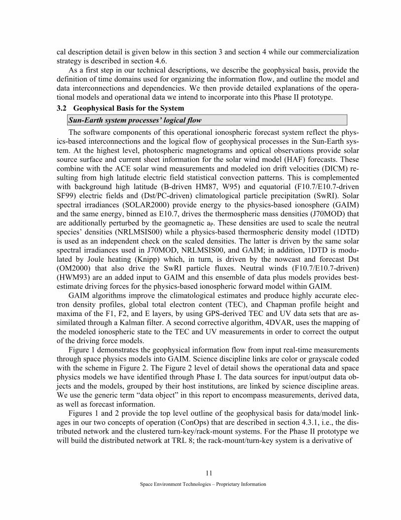
Sun-Earth system processes’ logical flow The software components of this operational ionospheric forecast system reflect the phys-
ics-based interconnections and the logical flow of geophysical processes in the Sun-Earth sys-tem. At the highest level, photospheric magnetograms and optical observations provide solar source surface and current sheet information for the solar wind model (HAF) forecasts. These combine with the ACE solar wind measurements and modeled ion drift velocities (DICM) re-sulting from high latitude electric field statistical convection patterns. This is complemented with background high latitude (B-driven HM87, W95) and equatorial (F10.7/E10.7-driven SF99) electric fields and (Dst/PC-driven) climatological particle precipitation (SwRI). Solar spectral irradiances (SOLAR2000) provide energy to the physics-based ionosphere (GAIM) and the same energy, binned as E10.7, drives the thermospheric mass densities (J70MOD) that are additionally perturbed by the geomagnetic aP. These densities are used to scale the neutral species’ densities (NRLMSIS00) while a physics-based thermospheric density model (1DTD) is used as an independent check on the scaled densities. The latter is driven by the same solar spectral irradiances used in J70MOD, NRLMSIS00, and GAIM; in addition, 1DTD is modu-lated by Joule heating (Knipp) which, in turn, is driven by the nowcast and forecast Dst (OM2000) that also drive the SwRI particle fluxes. Neutral winds (F10.7/E10.7-driven) (HWM93) are an added input to GAIM and this ensemble of data plus models provides best-estimate driving forces for the physics-based ionospheric forward model within GAIM.
GAIM algorithms improve the climatological estimates and produce highly accurate elec-tron density profiles, global total electron content (TEC), and Chapman profile height and maxima of the F1, F2, and E layers, by using GPS-derived TEC and UV data sets that are as-similated through a Kalman filter. A second corrective algorithm, 4DVAR, uses the mapping of the modeled ionospheric state to the TEC and UV measurements in order to correct the output of the driving force models.
Figure 1 demonstrates the geophysical information flow from input real-time measurements through space physics models into GAIM. Science discipline links are color or grayscale coded with the scheme in Figure 2. The Figure 2 level of detail shows the operational data and space physics models we have identified through Phase I. The data sources for input/output data ob-jects and the models, grouped by their host institutions, are linked by science discipline areas. We use the generic term “data object” in this report to encompass measurements, derived data, as well as forecast information.
Figures 1 and 2 provide the top level outline of the geophysical basis for data/model link-ages in our two concepts of operation (ConOps) that are described in section 4.3.1, i.e., the dis-tributed network and the clustered turn-key/rack-mount systems. For the Phase II prototype we will build the distributed network at TRL 8; the rack-mount/turn-key system is a derivative of

Space Environment Technologies – Proprietary Information
12
Figure 1. The Geophysical Information Flow from Input Real-Time Measurements through Space Physics Models into GAIM. Science Discipline Links are Color Coded (with Reference to Figure 2).
the distributed network and, as indicated in the Enhancement Program discussion, it will consti-tute the third year activity to move the system from TRL 8 to TRL 9.
In space weather characterization today, there is constant change. Therefore, in order to maximize advances in technology and physics or to take advantage of beneficial collaborations, we have modularly designed this system that links data and model objects. At the highest level, the Phase I operational system architecture has been designed so that the data communications superstructure is completely independent of any science model or data set. Linkage of the data I/O architecture to particular models and data occurs at lower levels using Unified Modeling Language (UML) protocols. 3.3 Time Domain Definition
A key element in achieving our prime objective of providing accurate nowcasts and reliable forecasts of ionospheric parameters is the organization of time into operationally useful do-mains. We define an operational time system that has a heritage in 3 decades of space weather characterization. Time domains are used to operationally designate the temporal interdepend-ence of physical space weather parameters that are relative to the current moment in time, i.e., “now.” The current moment in time is the key time marker in our system and is called the cur-rent epoch in the aerospace community; we have adopted that usage here.

Space Environment Technologies – Proprietary Information
13
Figure 2. The Data Sources for Input/Output Data Objects and the Models, Grouped by their Host Institutions, are Linked by Science Discipline Areas.

Space Environment Technologies – Proprietary Information
14
…graceful degradation… Relative to the current epoch, data contains information about the past, present, or future. In
addition, data can be considered primary or secondary in an operational system that uses re-dundant data streams to mitigate risks. We separate past, present, or future state information contained within data by using the nomenclature of historical, nowcast, or forecast for primary data stream information which has been enhanced. We use previous, current, or predicted for secondary data stream information which has a climatological quality. Using these time do-mains, failures in the primary (enhanced) data stream result in the use of secondary data stream (climatological) values; the overall effect is to maintain operational continuity in exchange for increased uncertainty. This concept is also known as “graceful degradation.” Section 4.3.2.4 (Classes) provides a detailed description of the use of these time domains in our software and hardware system.
Historical or previous data are operationally defined as that information older than 24 hours prior to the current epoch. These data have usually been measured, processed, reported (is-sued), and distributed by the organization that creates the information. Their values are unlikely to change significantly and they are ready for transfer to permanent archives.
Nowcast or current data are operationally defined as that information for the most recent 24 hour period, i.e., 24 hours ago up to the current epoch. Some measured data has been received by an operational system but it is likely that not all inputs for all models are yet available. Modeled data are often produced using multiple data sources which can include the most re-cently received input data and estimated (recently forecast) data. Their values are likely to change and they are not ready for transfer to permanent archives.
Forecast or predicted data are operationally defined as that information in the future relative to the current epoch. Forecast data have not been measured but only modeled from either first principles or empirical algorithms. Their values are extremely likely to change and they are not ready for transfer to permanent archives.
Hence, the values for particular types of data can be in a state of constant change. For op-erational purposes, the data creation date is not related to its designation as historical/previous, nowcast/current, or forecast/predicted. Historical/previous data tends to be measured, static, and ready for archival, nowcast/current data tends to be either modeled or measured but transi-tional, and forecast/predicted data tends to be modeled and mutable.
Figure 3 shows a graphical relationship between primary data stream historical, nowcast, and forecast time domains in combination with data uncertainty increasing through time. The secondary data stream is identical with the exception that previous, current, and predicted are the domain designations. This figure shows daily time granularity ranging from 48 hours in the past to 78 hours in the future and we use multiple time granularity over this time range. Time granularity is determined by the cadence of running models combined with the need for time information details.
Our time domain design has -48 to -24 hour data which allows models’ initialization, where necessary, with archival quality data. We extend the forecast time beyond 3 days to +78 hours in order to guarantee a minimum 72-hour forecast. Our operational time granularity includes 3-hour, 1-hour, and 15-minute data time steps with the real-time, highest time resolution centered on the current epoch ±1 hour.

Space Environment Technologies – Proprietary Information
15
3.4 Model and Data Dependencies The space physics models used by our system and the input data that drive them or the out-
put data they create, total 15 empirical or physics-based models and 25 data sets. Each has been selected for its operational or near-operational capability for use in this prototype project. The models and data streams will be verified at a TRL 6 (unit demonstration in near-operational environment) by the mid-point of year one and at TRL 7 (system demonstration in a relevant operational environment) in the first half of year 2 so that the complete prototype operational ionospheric forecast system can be demonstrated at TRL 8 (completed end-to-end system is tested, validated, and demonstrated in an operational environment) at the end of year 2.
Figures 1 and 2 show the top-level dependencies and linkages between the models and data streams. Table 3 summarizes the model input/output (I/O) parameters and their run cadences in minutes; they are listed in their approximate run-order. Light gray listings are anticipated mod-els or data sets. Table 4 lists the primary and secondary I/O parameters that are used to drive each of the models. Table 5 lists the user models, data input, producer models, data output, model creators, model host institutions, data creators, data host institutions, data stream IDs, as well as data and model TRL.
In Figures 4a-l, we show the next level of model and data dependencies. A key concept we use to guarantee operational robustness is that of “two streams” (see the risk management dis-cussion in section 4.3.5). The primary stream (“A,” coded blue or dark gray in Figures 4a-l) is the enhanced system data and information flow path. This stream provides the high time resolu-tion information and the local or regional detail of the ionosphere beyond climatology. It in-cludes the GOES-N EUV, SSN DCA, all ground- and space-based TEC, C/NOFS VEFI and NWM, SSULI UV, ACE IMF B, and ground-observed solar surface magnetograms as well as electromagnetic observations. The secondary stream (“B,” coded orange or medium gray) is the core information flow path and guarantees that the operational ionospheric forecast system pro-duces a climatological forecast in the event of enhanced component failures or data outages. It includes F10.7, Mg II cwr, Ap (ap, Kp), Dst, PC, Pe, and Pp.
Detail is provided in Figures 4a-l for the distributed network. Figure 4a gives the view of all components, Figure 4b shows the models and data stream, Figures 4c-d show the data base ac-cess, and Figures 4e-l show the eight science discipline areas of solar irradiances, neutral ther-mospheric densities, neutral thermospheric winds, high latitude heating, particle precipitation,
Figure 3. Representation of Primary Data Stream Historical, Nowcast, and Forecast Time Domains in Relation to the Current Epoch (“0”). The Uncertainty Inherent Within Data Sets is Shown as the Heavy Black Line and Time Granularity is Shown for 3-Hour, 1-Hour, and 15-Minute Data Time Steps.
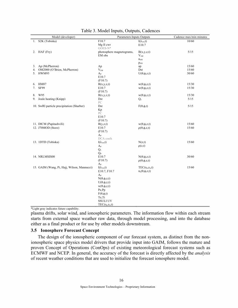
Space Environment Technologies – Proprietary Information
16
Table 3. Model Inputs, Outputs, Cadences Model (developer) Parameters Inputs Outputs Cadence max/min minutes
1. S2K (Tobiska) F10.7 Mg II cwr GOES-N*
I(λ39,t) E10.7
10/60
2. HAF (Fry) photosphere magnetograms, EM obs
B(x,y,z,t) VSW nSW pSW
5/15
3. Ap (McPherron) Ap ap 15/60 4. OM2000 (O’Brien, McPherron) VSW Dst 15/60 5. HWM93 AP
E10.7 (F10.7)
U(θ,φ,z,t) 30/60
6. HM87 B(x,y,z,t) w(θ,φ,z,t) 15/30 7. SF99 E10.7
(F10.7) w(θ,φ,z,t) 15/30
8. W95 B(x,y,z,t) w(θ,φ,z,t) 15/30 9. Joule heating (Knipp) Dst
PC QJ 5/15
10. SwRI particle precipitation (Sharber) Dst Kp PC E10.7 (F10.7)
F(θ,φ,t) 5/15
11. DICM (Papitashvili) B(y,z,t) w(θ,φ,z,t) 15/60 12. J70MOD (Storz) E10.7
(F10.7) AP DCA coefs
ρ(θ,φ,z,t) 15/60
13. 1DTD (Tobiska) I(λ39,t) AP QJ QP
N(z,t) ρ(z,t)
15/60
14. NRLMSIS00 E10.7 (F10.7) AP
N(θ,φ,z,t) ρ(θ,φ,z,t)
30/60
15. GAIM (Wang, Pi, Hajj, Wilson, Mannucci) I(λ39,t) E10.7, F10.7 AP N(θ,φ,z,t) U(θ,φ,z,t) w(θ,φ,z,t) Pe,Pp F(θ,φ,t) Te,Ti SSULI UV TEC(rR,rS,t)
TEC(rR,rS,t) ne(θ,φ,z,t)
15/60
*Light gray indicates future capability. plasma drifts, solar wind, and ionospheric parameters. The information flow within each stream starts from external space weather raw data, through model processing, and into the database either as a final product or for use by other models downstream. 3.5 Ionosphere Forecast Concept
The design of the ionospheric component of our forecast system, as distinct from the non-ionospheric space physics model drivers that provide input into GAIM, follows the mature and proven Concept of Operations (ConOps) of existing meteorological forecast systems such as ECMWF and NCEP. In general, the accuracy of the forecast is directly affected by the analysis of recent weather conditions that are used to initialize the forecast ionosphere model.

Space Environment Technologies – Proprietary Information
17
In the system ConOps, a balance between forecast ionosphere timeliness and accuracy leads to a design with an analysis schedule of multiple timescale granularities. These are near real-time (NRT), hourly (1H) and 3-hour (3H) analyses. The main differences between these analy-ses are the quantity of ionospheric observations assimilated to produce them. The two key pa-rameters affecting data availability are Data Collecting Window (DCW) and Cut-off Time (CT). For each analysis, data from a specified time interval is assimilated into the analysis model.
In order to produce analyses on schedule, a CT is specified for each analysis. The CT is the length of time after the DCW closes and before the start of analysis. The data collected in the
Table 4. Primary, Secondary I/O Parameters Parameter I/O Data Source User Model; mode*
Ap I O
NOAA SEC McPherron
HWM93, J70MOD, 1DTD,GAIM, MSIS; H,N,F
B(x,y,z,t) I O
ACE HAF
DICM, HM87, W95; H,N,F
DCA coefs I SSN J70MOD; N,F Dst O
I WDC-C2 OM2000
SwRI, Joule heating; H,N,F
E10.7 O I
S2K SwRI, HWM93, J70MOD, GAIM, MSIS, SF99; H,N,F
EM obs I NOAA SEC HAF; N,F F(θ,φ,t) O
I SwRI GAIM; H,N,F
F10.7 I NOAA SEC SET
S2K, SwRI, HWM93, J70MOD, GAIM, MSIS, SF99; H,N,F
GOES-N I NOAA SEC S2K; N,F I(λ39,t) O
I S2K 1DTD, GAIM; H,N,F
Kp I NOAA SEC SwRI; H,N,F Mg II cwr I NOAA SEC
SET S2K; H,N,F
N(θ,φ,z,t) O I
(1DTD,) MSIS
GAIM; H,N,F
ne(θ,φ,z,t) O GAIM users; H,N,F PC I WDC-C2 SwRI, Joule heating; H magnetogram I NOAA SEC HAF; N,F Pe, Pp, QP I NOAA SEC GAIM, 1DTD; H,N φ I
O geometry - mag long, local time DICM, GAIM, SwRI, HWM93, J70MOD, MSIS, SF99, W95, HM87;
H,N,F QJ O
I Knipp 1DTD; H,N,F
ρ(θ,φ,z,t) O J70MOD (1DTD, MSIS); H,N,F SSULI UV I DMSP GAIM; H,N t I
O UT clock - Time all models, data sets, parameters; H,N,F
Te O GAIM GAIM; H,N,F TEC(rR,rS,t) I
O JPL GPS, CORS, C/N CORISS GAIM; H,N,F
Ti O GAIM GAIM; H,N,F θ I
O geometry - magnetic latitude DICM, GAIM, SwRI, HWM93, J70MOD, MSIS, SF99, W95, HM87;
H,N,F U(θ,φ,z,t) O
I HWM93 C/N NWM
GAIM; H,N,F
VSW O I
ACE, HAF
OM2000; H,N,F
w(θ,φ,z,t) O I
DICM, C/N VEFI, SF99, W95, HM87 GAIM; H,N,F
z O geometry - altitude DICM, HWM93, J70MOD, 1DTD, GAIM, MSIS, SF99, W95, HM87, SwRI; H,N,F
*H = historical; N = nowcast; F = forecast; light gray indicates future capability.
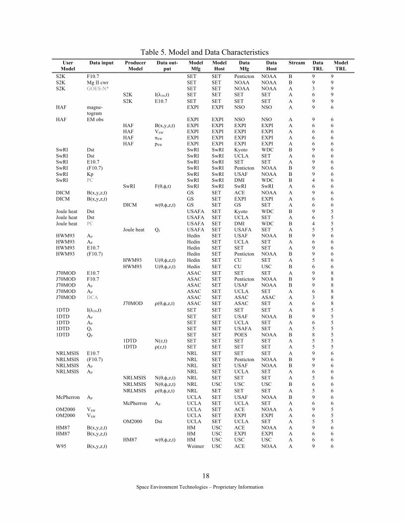
Space Environment Technologies – Proprietary Information
18
Table 5. Model and Data Characteristics User
Model Data input Producer
Model Data out-
put Model Mfg
Model Host
Data Mfg
Data Host
Stream Data TRL
Model TRL
S2K F10.7 SET SET Penticton NOAA B 9 9 S2K Mg II cwr SET SET NOAA NOAA B 9 9 S2K GOES-N* SET SET NOAA NOAA A 3 9 S2K I(λ39,t) SET SET SET SET A 6 9 S2K E10.7 SET SET SET SET A 9 9 HAF magne-
togram EXPI EXPI NSO NSO A 9 6
HAF EM obs EXPI EXPI NSO NSO A 9 6 HAF B(x,y,z,t) EXPI EXPI EXPI EXPI A 6 6 HAF VSW EXPI EXPI EXPI EXPI A 6 6 HAF nSW EXPI EXPI EXPI EXPI A 6 6 HAF pSW EXPI EXPI EXPI EXPI A 6 6 SwRI Dst SwRI SwRI Kyoto WDC B 9 6 SwRI Dst SwRI SwRI UCLA SET A 6 6 SwRI E10.7 SwRI SwRI SET SET A 9 6 SwRI (F10.7) SwRI SwRI Penticton NOAA B 9 6 SwRI Kp SwRI SwRI USAF NOAA B 9 6 SwRI PC SwRI SwRI DMI WDC B 4 6 SwRI F(θ,φ,t) SwRI SwRI SwRI SwRI A 6 6 DICM B(x,y,z,t) GS SET ACE NOAA A 9 6 DICM B(x,y,z,t) GS SET EXPI EXPI A 6 6 DICM w(θ,φ,z,t) GS SET GS SET A 6 6 Joule heat Dst USAFA SET Kyoto WDC B 9 5 Joule heat Dst USAFA SET UCLA SET A 6 5 Joule heat PC USAFA SET DMI WDC B 4 5 Joule heat QJ USAFA SET USAFA SET A 5 5 HWM93 AP Hedin SET USAF NOAA B 9 6 HWM93 AP Hedin SET UCLA SET A 6 6 HWM93 E10.7 Hedin SET SET SET A 9 6 HWM93 (F10.7) Hedin SET Penticton NOAA B 9 6 HWM93 U(θ,φ,z,t) Hedin SET CU SET A 5 6 HWM93 U(θ,φ,z,t) Hedin SET CU USC B 6 6 J70MOD E10.7 ASAC SET SET SET A 9 8 J70MOD F10.7 ASAC SET Penticton NOAA B 9 8 J70MOD AP ASAC SET USAF NOAA B 9 8 J70MOD AP ASAC SET UCLA SET A 6 8 J70MOD DCA ASAC SET ASAC ASAC A 3 8 J70MOD ρ(θ,φ,z,t) ASAC SET ASAC SET A 6 8 1DTD I(λ39,t) SET SET SET SET A 8 5 1DTD AP SET SET USAF NOAA B 9 5 1DTD AP SET SET UCLA SET A 6 5 1DTD QJ SET SET USAFA SET A 5 5 1DTD QP SET SET POES NOAA B 8 5 1DTD N(z,t) SET SET SET SET A 5 5 1DTD ρ(z,t) SET SET SET SET A 5 5 NRLMSIS E10.7 NRL SET SET SET A 9 6 NRLMSIS (F10.7) NRL SET Penticton NOAA B 9 6 NRLMSIS AP NRL SET USAF NOAA B 9 6 NRLMSIS AP NRL SET UCLA SET A 6 6 NRLMSIS N(θ,φ,z,t) NRL SET SET SET A 5 6 NRLMSIS N(θ,φ,z,t) NRL USC USC USC B 6 6 NRLMSIS ρ(θ,φ,z,t) NRL SET SET SET A 5 6 McPherron AP UCLA SET USAF NOAA B 9 6 McPherron AP UCLA SET UCLA SET A 6 6 OM2000 VSW UCLA SET ACE NOAA A 9 5 OM2000 VSW UCLA SET EXPI EXPI A 6 5 OM2000 Dst UCLA SET UCLA SET A 5 5 HM87 B(x,y,z,t) HM USC ACE NOAA A 9 6 HM87 B(x,y,z,t) HM USC EXPI EXPI A 6 6 HM87 w(θ,φ,z,t) HM USC USC USC A 6 6 W95 B(x,y,z,t) Weimer USC ACE NOAA A 9 6
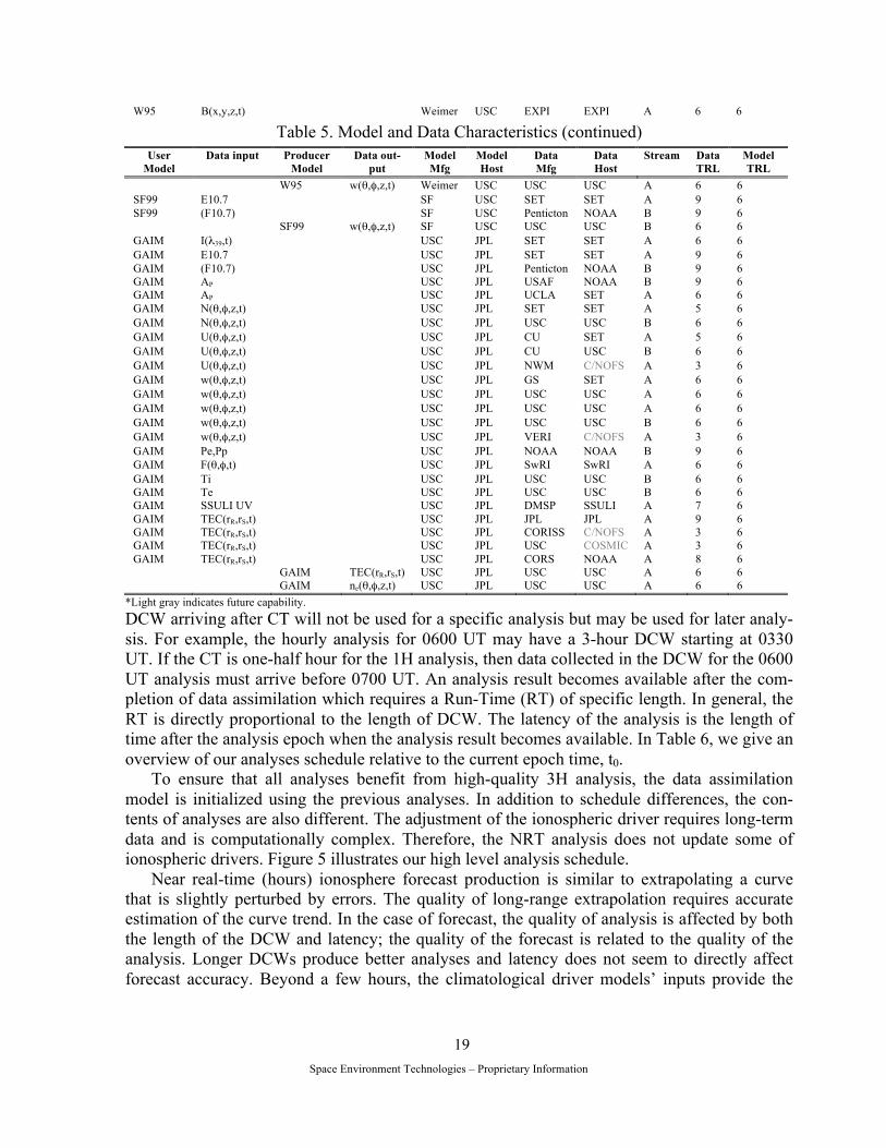
Space Environment Technologies – Proprietary Information
19
W95 B(x,y,z,t) Weimer USC EXPI EXPI A 6 6
Table 5. Model and Data Characteristics (continued) User
Model Data input Producer
Model Data out-
put Model Mfg
Model Host
Data Mfg
Data Host
Stream Data TRL
Model TRL
W95 w(θ,φ,z,t) Weimer USC USC USC A 6 6 SF99 E10.7 SF USC SET SET A 9 6 SF99 (F10.7) SF USC Penticton NOAA B 9 6 SF99 w(θ,φ,z,t) SF USC USC USC B 6 6 GAIM I(λ39,t) USC JPL SET SET A 6 6 GAIM E10.7 USC JPL SET SET A 9 6 GAIM (F10.7) USC JPL Penticton NOAA B 9 6 GAIM AP USC JPL USAF NOAA B 9 6 GAIM AP USC JPL UCLA SET A 6 6 GAIM N(θ,φ,z,t) USC JPL SET SET A 5 6 GAIM N(θ,φ,z,t) USC JPL USC USC B 6 6 GAIM U(θ,φ,z,t) USC JPL CU SET A 5 6 GAIM U(θ,φ,z,t) USC JPL CU USC B 6 6 GAIM U(θ,φ,z,t) USC JPL NWM C/NOFS A 3 6 GAIM w(θ,φ,z,t) USC JPL GS SET A 6 6 GAIM w(θ,φ,z,t) USC JPL USC USC A 6 6 GAIM w(θ,φ,z,t) USC JPL USC USC A 6 6 GAIM w(θ,φ,z,t) USC JPL USC USC B 6 6 GAIM w(θ,φ,z,t) USC JPL VERI C/NOFS A 3 6 GAIM Pe,Pp USC JPL NOAA NOAA B 9 6 GAIM F(θ,φ,t) USC JPL SwRI SwRI A 6 6 GAIM Ti USC JPL USC USC B 6 6 GAIM Te USC JPL USC USC B 6 6 GAIM SSULI UV USC JPL DMSP SSULI A 7 6 GAIM TEC(rR,rS,t) USC JPL JPL JPL A 9 6 GAIM TEC(rR,rS,t) USC JPL CORISS C/NOFS A 3 6 GAIM TEC(rR,rS,t) USC JPL USC COSMIC A 3 6 GAIM TEC(rR,rS,t) USC JPL CORS NOAA A 8 6 GAIM TEC(rR,rS,t) USC JPL USC USC A 6 6 GAIM ne(θ,φ,z,t) USC JPL USC USC A 6 6
*Light gray indicates future capability. DCW arriving after CT will not be used for a specific analysis but may be used for later analy-sis. For example, the hourly analysis for 0600 UT may have a 3-hour DCW starting at 0330 UT. If the CT is one-half hour for the 1H analysis, then data collected in the DCW for the 0600 UT analysis must arrive before 0700 UT. An analysis result becomes available after the com-pletion of data assimilation which requires a Run-Time (RT) of specific length. In general, the RT is directly proportional to the length of DCW. The latency of the analysis is the length of time after the analysis epoch when the analysis result becomes available. In Table 6, we give an overview of our analyses schedule relative to the current epoch time, t0.
To ensure that all analyses benefit from high-quality 3H analysis, the data assimilation model is initialized using the previous analyses. In addition to schedule differences, the con-tents of analyses are also different. The adjustment of the ionospheric driver requires long-term data and is computationally complex. Therefore, the NRT analysis does not update some of ionospheric drivers. Figure 5 illustrates our high level analysis schedule.
Near real-time (hours) ionosphere forecast production is similar to extrapolating a curve that is slightly perturbed by errors. The quality of long-range extrapolation requires accurate estimation of the curve trend. In the case of forecast, the quality of analysis is affected by both the length of the DCW and latency; the quality of the forecast is related to the quality of the analysis. Longer DCWs produce better analyses and latency does not seem to directly affect forecast accuracy. Beyond a few hours, the climatological driver models’ inputs provide the
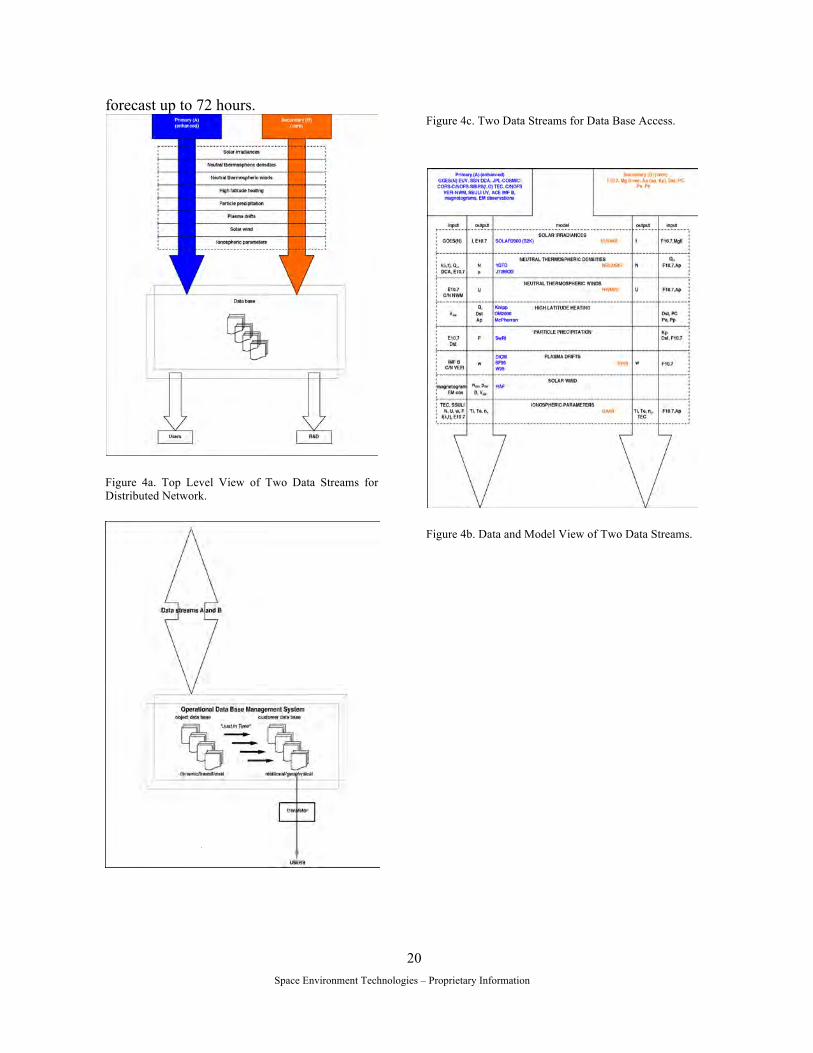
Space Environment Technologies – Proprietary Information
20
forecast up to 72 hours.
Figure 4a. Top Level View of Two Data Streams for Distributed Network.
Figure 4c. Two Data Streams for Data Base Access.
Figure 4b. Data and Model View of Two Data Streams.

Space Environment Technologies – Proprietary Information
21
Figure 4d. User Access Out of Database.
Figure 4e. Two Data Streams for Solar Irradiances.
Figure 4g. Two Data Streams for Neutral Thermospheric Winds.
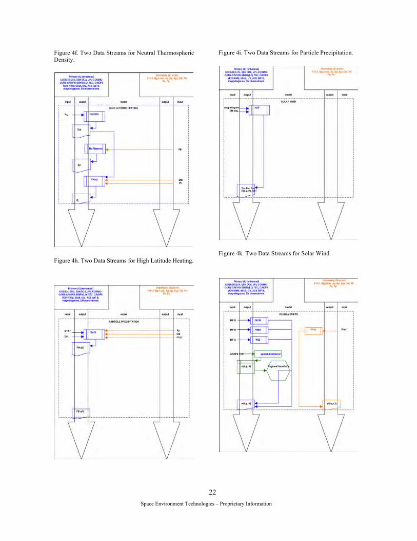
Space Environment Technologies – Proprietary Information
22
Figure 4f. Two Data Streams for Neutral Thermospheric Density.
Figure 4h. Two Data Streams for High Latitude Heating.
Figure 4i. Two Data Streams for Particle Precipitation.
Figure 4k. Two Data Streams for Solar Wind.
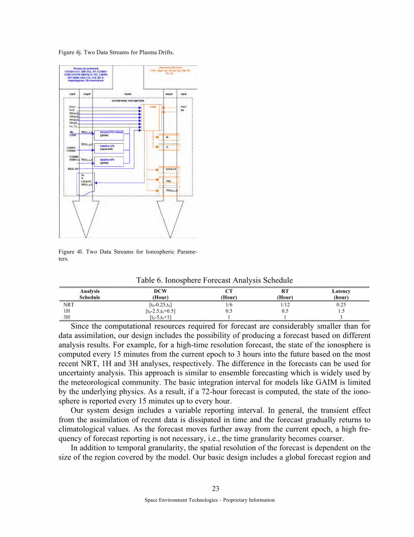
Space Environment Technologies – Proprietary Information
23
Figure 4j. Two Data Streams for Plasma Drifts.
Figure 4l. Two Data Streams for Ionospheric Parame-ters.
Table 6. Ionosphere Forecast Analysis Schedule
Analysis Schedule
DCW (Hour)
CT (Hour)
RT (Hour)
Latency (hour)
NRT [t0-0.25,t0] 1/6 1/12 0.25 1H [t0-2.5,t0+0.5] 0.5 0.5 1.5 3H [t0-5,t0+1] 1 1 3
Since the computational resources required for forecast are considerably smaller than for data assimilation, our design includes the possibility of producing a forecast based on different analysis results. For example, for a high-time resolution forecast, the state of the ionosphere is computed every 15 minutes from the current epoch to 3 hours into the future based on the most recent NRT, 1H and 3H analyses, respectively. The difference in the forecasts can be used for uncertainty analysis. This approach is similar to ensemble forecasting which is widely used by the meteorological community. The basic integration interval for models like GAIM is limited by the underlying physics. As a result, if a 72-hour forecast is computed, the state of the iono-sphere is reported every 15 minutes up to every hour.
Our system design includes a variable reporting interval. In general, the transient effect from the assimilation of recent data is dissipated in time and the forecast gradually returns to climatological values. As the forecast moves further away from the current epoch, a high fre-quency of forecast reporting is not necessary, i.e., the time granularity becomes coarser.
In addition to temporal granularity, the spatial resolution of the forecast is dependent on the size of the region covered by the model. Our basic design includes a global forecast region and
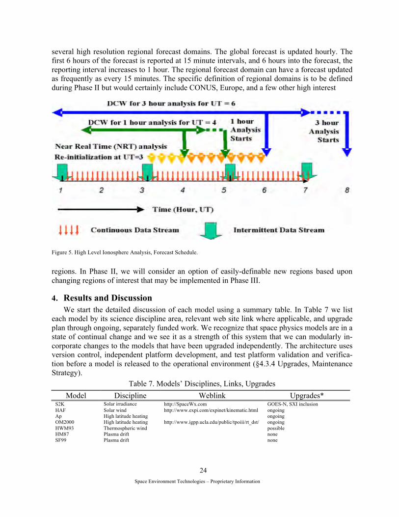
Space Environment Technologies – Proprietary Information
24
several high resolution regional forecast domains. The global forecast is updated hourly. The first 6 hours of the forecast is reported at 15 minute intervals, and 6 hours into the forecast, the reporting interval increases to 1 hour. The regional forecast domain can have a forecast updated as frequently as every 15 minutes. The specific definition of regional domains is to be defined during Phase II but would certainly include CONUS, Europe, and a few other high interest
Figure 5. High Level Ionosphere Analysis, Forecast Schedule.
regions. In Phase II, we will consider an option of easily-definable new regions based upon changing regions of interest that may be implemented in Phase III.
4. Results and Discussion We start the detailed discussion of each model using a summary table. In Table 7 we list
each model by its science discipline area, relevant web site link where applicable, and upgrade plan through ongoing, separately funded work. We recognize that space physics models are in a state of continual change and we see it as a strength of this system that we can modularly in-corporate changes to the models that have been upgraded independently. The architecture uses version control, independent platform development, and test platform validation and verifica-tion before a model is released to the operational environment (§4.3.4 Upgrades, Maintenance Strategy).
Table 7. Models’ Disciplines, Links, Upgrades Model Discipline Weblink Upgrades*
S2K Solar irradiance http://SpaceWx.com GOES-N, SXI inclusion HAF Solar wind http://www.expi.com/expinet/kinematic.html ongoing Ap High latitude heating ongoing OM2000 High latitude heating http://www.igpp.ucla.edu/public/tpoiii/rt_dst/ ongoing HWM93 Thermospheric wind possible HM87 Plasma drift none SF99 Plasma drift none
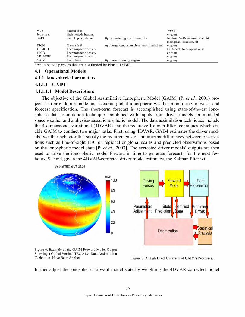
Space Environment Technologies – Proprietary Information
25
W95 Plasma drift W03 (?) Joule heat High latitude heating ongoing SwRI Particle precipitation http://climatology.space.swri.edu/ NOAA-15,-16 inclusion and Dst
main phase, recovery fit DICM Plasma drift http://maggy.engin.umich.edu/mist/limie.html ongoing J70MOD Thermospheric density DCA coefs to be operational 1DTD Thermospheric density ongoing NRLMSIS Thermospheric density ongoing GAIM Ionosphere http://iono.jpl.nasa.gov/gaim ongoing
*Anticipated upgrades that are not funded by Phase II SBIR.
4.1 Operational Models 4.1.1 Ionospheric Parameters 4.1.1.1 GAIM 4.1.1.1.1 Model Description:
The objective of the Global Assimilative Ionospheric Model (GAIM) (Pi et al., 2001) pro-ject is to provide a reliable and accurate global ionospheric weather monitoring, nowcast and forecast specification. The short-term forecast is accomplished using state-of-the-art iono-spheric data assimilation techniques combined with inputs from driver models for modeled space weather and a physics-based ionospheric model. The data assimilation techniques include the 4-dimensional variational (4DVAR) and the recursive Kalman filter techniques which en-able GAIM to conduct two major tasks. First, using 4DVAR, GAIM estimates the driver mod-els’ weather behavior that satisfy the requirements of minimizing differences between observa-tions such as line-of-sight TEC on regional or global scales and predicted observations based on the ionospheric model state [Pi et al., 2003]. The corrected driver models’ outputs are then used to drive the ionospheric model forward in time to generate forecasts for the next few hours. Second, given the 4DVAR-corrected driver model estimates, the Kalman filter will
Figure 6. Example of the GAIM Forward Model Output Showing a Global Vertical TEC After Data Assimilation Techniques Have Been Applied.
Figure 7. A High Level Overview of GAIM’s Processes.
further adjust the ionospheric forward model state by weighting the 4DVAR-corrected model
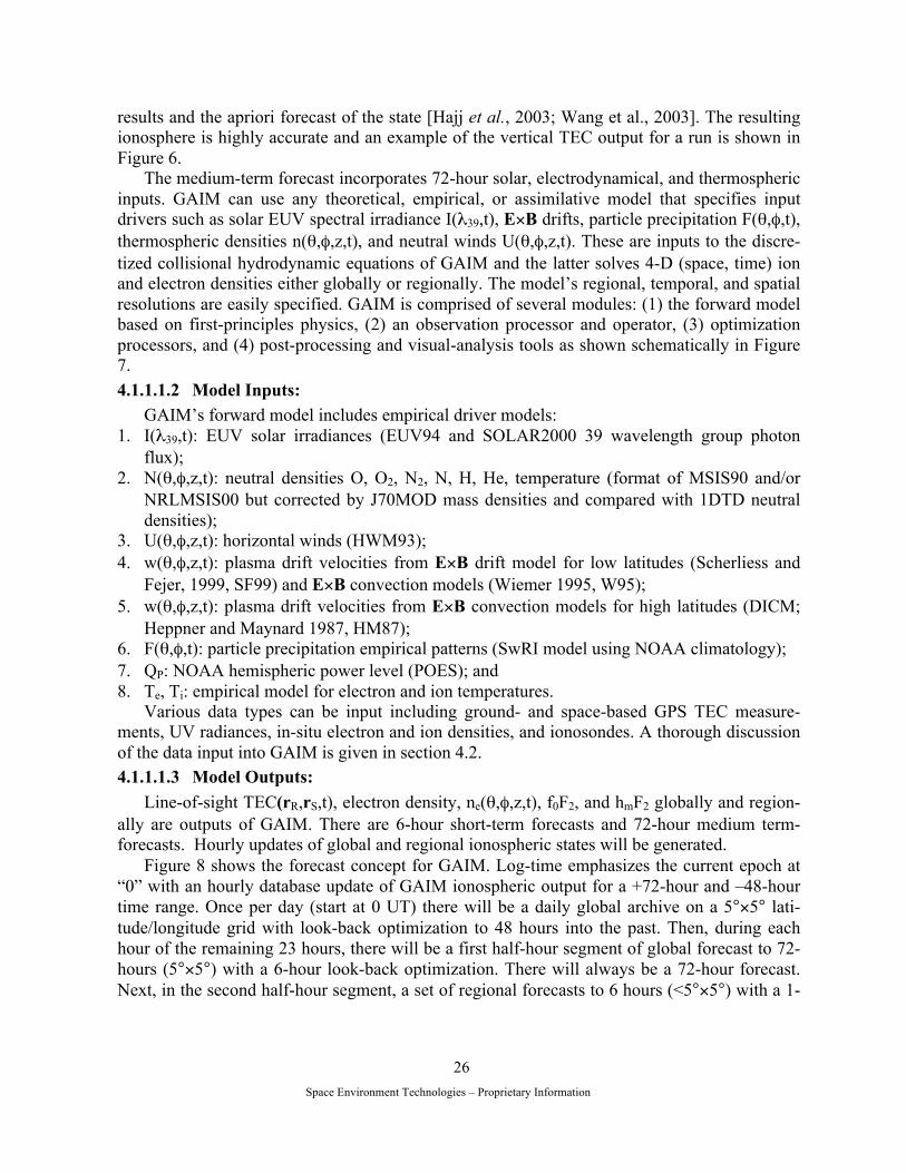
Space Environment Technologies – Proprietary Information
26
results and the apriori forecast of the state [Hajj et al., 2003; Wang et al., 2003]. The resulting ionosphere is highly accurate and an example of the vertical TEC output for a run is shown in Figure 6.
The medium-term forecast incorporates 72-hour solar, electrodynamical, and thermospheric inputs. GAIM can use any theoretical, empirical, or assimilative model that specifies input drivers such as solar EUV spectral irradiance I(λ39,t), E×B drifts, particle precipitation F(θ,φ,t), thermospheric densities n(θ,φ,z,t), and neutral winds U(θ,φ,z,t). These are inputs to the discre-tized collisional hydrodynamic equations of GAIM and the latter solves 4-D (space, time) ion and electron densities either globally or regionally. The model’s regional, temporal, and spatial resolutions are easily specified. GAIM is comprised of several modules: (1) the forward model based on first-principles physics, (2) an observation processor and operator, (3) optimization processors, and (4) post-processing and visual-analysis tools as shown schematically in Figure 7. 4.1.1.1.2 Model Inputs:
GAIM’s forward model includes empirical driver models: 1. I(λ39,t): EUV solar irradiances (EUV94 and SOLAR2000 39 wavelength group photon
flux); 2. N(θ,φ,z,t): neutral densities O, O2, N2, N, H, He, temperature (format of MSIS90 and/or
NRLMSIS00 but corrected by J70MOD mass densities and compared with 1DTD neutral densities);
3. U(θ,φ,z,t): horizontal winds (HWM93); 4. w(θ,φ,z,t): plasma drift velocities from E×B drift model for low latitudes (Scherliess and
Fejer, 1999, SF99) and E×B convection models (Wiemer 1995, W95); 5. w(θ,φ,z,t): plasma drift velocities from E×B convection models for high latitudes (DICM;
Heppner and Maynard 1987, HM87); 6. F(θ,φ,t): particle precipitation empirical patterns (SwRI model using NOAA climatology); 7. QP: NOAA hemispheric power level (POES); and 8. Te, Ti: empirical model for electron and ion temperatures.
Various data types can be input including ground- and space-based GPS TEC measure-ments, UV radiances, in-situ electron and ion densities, and ionosondes. A thorough discussion of the data input into GAIM is given in section 4.2. 4.1.1.1.3 Model Outputs:
Line-of-sight TEC(rR,rS,t), electron density, ne(θ,φ,z,t), f0F2, and hmF2 globally and region-ally are outputs of GAIM. There are 6-hour short-term forecasts and 72-hour medium term-forecasts. Hourly updates of global and regional ionospheric states will be generated.
Figure 8 shows the forecast concept for GAIM. Log-time emphasizes the current epoch at “0” with an hourly database update of GAIM ionospheric output for a +72-hour and –48-hour time range. Once per day (start at 0 UT) there will be a daily global archive on a 5°×5° lati-tude/longitude grid with look-back optimization to 48 hours into the past. Then, during each hour of the remaining 23 hours, there will be a first half-hour segment of global forecast to 72-hours (5°×5°) with a 6-hour look-back optimization. There will always be a 72-hour forecast. Next, in the second half-hour segment, a set of regional forecasts to 6 hours (<5°×5°) with a 1-

Space Environment Technologies – Proprietary Information
27
hour look-back optimization will be run. GAIM will use, as its input, the output from each of the other models at their own geo-
physical cadence. GAIM outputs for the global archive are written for each 3-hour time seg-ment; for the hourly global run there will be ionospheric output every 1-hour time segment. For the regional hourly run, there will be output every 15 minutes the first hour then hourly out to 6 hours. Output data overlaid (inserted) into the database time slots will be the updated method.
Figure 8. GAIM Forecast Timeline in Log-Time (-48 to +72 Hours).
There are several options to reduce compute time and they include:
1. add processors; 2. rotate regions (every 2-3 hours); 3. change latitude/longitude bin size; 4. change definition of region size; 5. limit the number of regions; and 6. change the number of look-back hours for optimization.
We expect that the distributed network prototype system will demonstrate a subset of these options; extensibility and scalability will be options for a TRL 9 operational system. 4.1.2 Solar Wind 4.1.2.1 HAF 4.1.2.1.1 Model Description:
The Hakamada-Akasofu-Fry (HAF) Solar Wind Model was developed by the Geophysical Institute, University of Alaska, Fairbanks (GI/UAF) and Exploration Physics International, Inc. (EXPI). The HAF model provides quantitative forecasts, days in advance, of solar wind condi-tions. Specifically, it tracks interplanetary disturbances as they propagate from their source at the Sun. HAF also provides temporal profiles of the solar wind speed, density, dynamic pres-sure, and Interplanetary Magnetic Field (IMF) anywhere in the solar system.
The HAF model is driven using synoptic solar observations and solar event reports. This in-

Space Environment Technologies – Proprietary Information
28
formation is used to predict the timing and severity of space weather disturbances following solar events, or the passage of Co-rotating Interaction Regions (CIR). The HAF model maps the disturbed and the undisturbed solar wind, so it is applicable to all phases of the solar cycle. Additionally, HAF produces chronological sequences of ecliptic-plane plots of the IMF and other solar wind parameters (Figure 9).
The HAF kinematic procedure follows fluid parcels and the frozen-in IMF field lines. This approach to first principles conserves mass and momentum but not energy. This methodology is described by Hakamada and Akasofu (1982), Fry (1985), Akasofu (2001) and Fry et al. (2001, 2003) (Figure 10). The HAF model internal parameters have been calibrated with a 1-D MHD model (Sun et al., 1985; Dryer, 1994). Recent model improvements are described in Fry et al. (2001) and validation of the model is discussed in Fry et al. (2003). Eventually, HAF would form part of, or even be replaced by, a hybrid system that includes the HAF model and a first principles 3D MHD model as envisioned by Dryer (1994, 1998) and Detman (private communication, 2002). 4.1.2.1.2 Model Inputs:
Ambient Solar Wind (vector magnetograms) and Event-Driven Solar Wind (EM observa-tions).
Ambient Solar Wind: Input for the “non-event” background solar wind is provided by solar surface magnetograms (vector magnetograms) (from the National Solar observatory, Tucson, AZ) that are utilized to construct a potential field coronal magnetic field model. This model is then used to build a map of the radial IMF and velocity (Wang and Sheeley, 1990; Arge and Pizzo, 2000) at a spherical “source surface” at 2.5 RS (where RS is the solar radius and is equal to 6.9 × 10⁶ km). These inner boundary conditions are then used to initialize the kinematic HAF
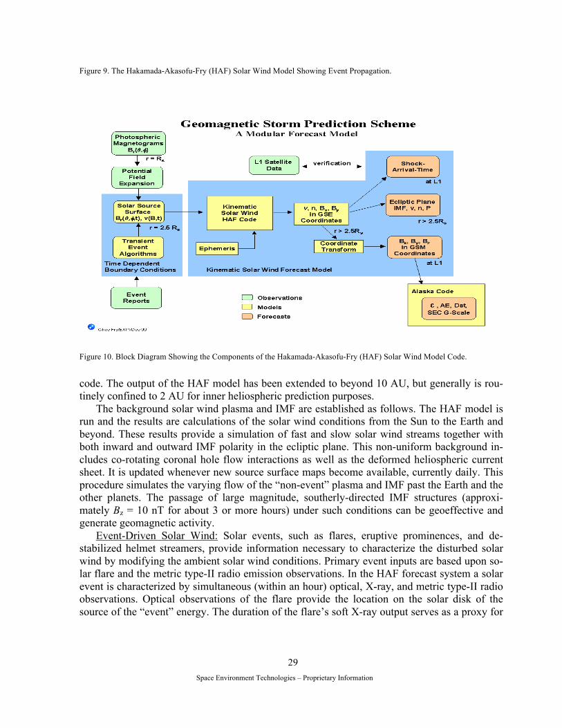
Space Environment Technologies – Proprietary Information
29
Figure 9. The Hakamada-Akasofu-Fry (HAF) Solar Wind Model Showing Event Propagation.
Figure 10. Block Diagram Showing the Components of the Hakamada-Akasofu-Fry (HAF) Solar Wind Model Code.
code. The output of the HAF model has been extended to beyond 10 AU, but generally is rou-tinely confined to 2 AU for inner heliospheric prediction purposes.
The background solar wind plasma and IMF are established as follows. The HAF model is run and the results are calculations of the solar wind conditions from the Sun to the Earth and beyond. These results provide a simulation of fast and slow solar wind streams together with both inward and outward IMF polarity in the ecliptic plane. This non-uniform background in-cludes co-rotating coronal hole flow interactions as well as the deformed heliospheric current sheet. It is updated whenever new source surface maps become available, currently daily. This procedure simulates the varying flow of the “non-event” plasma and IMF past the Earth and the other planets. The passage of large magnitude, southerly-directed IMF structures (approxi-mately Bz = 10 nT for about 3 or more hours) under such conditions can be geoeffective and generate geomagnetic activity.
Event-Driven Solar Wind: Solar events, such as flares, eruptive prominences, and de-stabilized helmet streamers, provide information necessary to characterize the disturbed solar wind by modifying the ambient solar wind conditions. Primary event inputs are based upon so-lar flare and the metric type-II radio emission observations. In the HAF forecast system a solar event is characterized by simultaneous (within an hour) optical, X-ray, and metric type-II radio observations. Optical observations of the flare provide the location on the solar disk of the source of the “event” energy. The duration of the flare’s soft X-ray output serves as a proxy for

Space Environment Technologies – Proprietary Information
30
the shock’s piston-driving time. The metric type-II radio burst observation, coupled with a cor-onal density model, provides an estimate of the initial coronal shock speed, Vs, the magnitude of which is assumed to be related to the solar disturbance’s energy output. These optical, radio, and X-ray observations (EM observations) are provided on a real-time basis by the U.S. Air Force Weather Agency and the NOAA Space Environment Center. Table 8 lists the HAF model inputs and associated data sources. 4.1.2.1.3 Model Outputs:
The model produces IMF B(x,y,z,t), Temporal Profiles of Solar Wind Parameters, Eclip-tic/Equatorial Plane Displays, and Shock Arrival Time.
Temporal Profiles of Solar Wind Parameters: HAF predicts values of specific physical pa-rameters, such as plasma velocity, V, IMF magnitude and polarity (B and, in particular, Bz), density, n, and dynamic pressure, p, at one-hour time steps extending 5–27 days into the future.
Ecliptic/Equatorial Plane Displays: The forecaster can examine an ecliptic plane figure pro-vided by HAF that shows the co-rotating flow and IMF during the “pre-event” specification of plasma and IMF background. Following the “event,” the forecaster can examine the temporal and spatial evolution of the propagating Interplanetary Coronal Mass Ejection (ICME) together with its shock. Displays include the predicted IMF configuration and the location of Earth (spe-cifically at the L1 spacecraft location) in the ecliptic plane and of Mars (for calibration and re-search purposes) at 12-hour intervals for 5 days into the future.
Shock Arrival Time: The predicted Shock Arrival Time (SAT) is determined by computing a Shock Searching Index (SSI). The SSI is equal to the logarithm (base 10) of the model’s dy-namic pressure change, normalized to the pre-disturbed dynamic pressure, at each time step. The event’s shock arrival time is predicted when this SSI reaches an empirically determined threshold value (currently SSI= -0.35). If this SSI threshold is not achieved, the shock is
Table 8. Data Sources for HAF Solar Wind Model Input Parameter Data Source/
Observation Instrument/ Observatory
OPR When Updated Desired Resolution
Status*
Simulation start time Forecaster or auto - Fore-caster
Scheduled or event 15 minutes 1
Ambient solar wind: a. Inner boundary magnetic field grid
Photospheric magnetic field
WSO, MWO, NSO ISOON
NOAA SEC RPC
Automatic, once or twice-daily
5°×5° (HAF v2); 1°×1° (HAF v3)
1 1
b. Inner boundary ve-locity grid
Empirical algorithm Derived from 2a
UAF/GI Same as 2a Same as 2a 1
c. Inner boundary density grid
Empirical algorithm Derived from 2a
UAF/GI Same as 2a Same as 2a 1
Events: a. Time event began X-ray flux, Type II thresh-
old GOES X-ray, SXI
NOAA SEC
Receipt of report 5 minutes 1,2
b. Time event maxi-mum
X-ray flux peak GOES X-ray, SXI
NOAA SEC
Receipt of report 5 minutes 1,2
c. Time event end X-ray flux drops to 1/2 max on log plot
GOES X-ray, SXI
NOAA SEC
Receipt of report 5 minutes 1,2
d. Heliolatitude of event source location
Hα flare location; X-ray, radio source loca-tion
SOON; GOES SXI
USAF Receipt of report 5° (HAF v2) 1° (HAF v3)
1 1,2
e. Heliolongitude of event source location
Hα flare location; X-ray, radio source loca-tion
SOON; GOES SXI
USAF Receipt of report 5° (HAF v2) 1° (HAF v3)
1 1,2

Space Environment Technologies – Proprietary Information
31
f. Initial shock speed Type II Shock Speed SOON, SFIR; SRS
USAF Receipt of report 50 km/sec 1
g. Shock shape pa-rameter
Shock angular width From 3a,b,c,for free parameter
UAF/GI At report time 10 degrees 1/3
*Status: 1 = Presently operational; 2 = Scheduled; 3 = Required but not planned declared to have decayed to an MHD wave by the time the disturbance reaches the Earth’s lo-cation. By comparing HAF model results with ACE and/or SOHO observations, the prediction error is then the time difference, i.e., the prediction time minus the observed SAT. Predicted shock arrival time, when compared with ACE spacecraft observations, provides a metric for evaluating model performance and demonstrates the “goodness” of solar wind parameter tem-poral profiles modeled by HAF. The model RMS error is presently about ±12 hours. We note that the inclusion of real-time ACE data substantially improves the actual shock arrival time estimation. 4.1.3 Plasma Drifts 4.1.3.1 DICM 4.1.3.1.1 Model Description:
The DMSP-based Ionospheric Convection Model (DICM) (Papitashvili et al., 1994, 1998, 1999, 2002) uses the ionospheric electrostatic potentials for its construction which have been inferred from the cross-track thermal ion drift velocity measurements made onboard of the DMSP satellites F8 and F10-F13 in 1993-1996. These satellite measurements and the simulta-neous observations of the Solar Wind (SW) and Interplanetary Magnetic Field (IMF) condi-tions near the Earth’s orbit have been correlated to create an empirical model of the high-latitude electric potential patterns for various IMF/SW conditions. As a result, DICM is fully parameterized by the IMF strength and directions and constructed for different seasons (sum-mer, equinox, and winter). Running this model, ionospheric convection patterns are generated for any given IMF configuration for quiet-to-moderate geomagnetic activity conditions (Figure 11). New elements in DICM are its “quasi-viscous” patterns for IMF ~0 and separate, IMF-dependent patterns constructed for both northern and southern polar regions which are not available in other ionospheric convection models. 4.1.3.1.2 Model Inputs:
The model uses B(y,z,t) and time as inputs. Control parameters include the transverse orien-tation of the interplanetary magnetic field By, Bz (in GSM coordinates), and the orientation of the Earth’s magnetic axis (season) at the time of interest. These parameters are used to set up the model for the desired conditions. Time is input in ISO standard format of YYYY-MM-DD hh:mm:ss.fff.

Space Environment Technologies – Proprietary Information
32
4.1.3.1.3 Model Outputs:
Figure 11. DICM Model Output Where the Contoured Electric Fields are Turned Into Ion Drift Velocities.
The output from the model is the plasma drift velocity, w(θ,φ,z,t), in the form of iono-
spheric electrostatic potential maps, in kilovolts (kV), constructed either as a function of the corrected geomagnetic (CGM) latitude and magnetic local time (MLT), or in geographic coor-dinates for given universal time (UT). The output file is flat ASCII, approximately 8 kB for each time step, in latitude (y-axis) and MLT (x-axis). 4.1.3.2 W95 4.1.3.2.1 Model Description:
The E×B convection models for high latitudes (Weimer, 1995; Weimer et al., 2003) is em-bedded within the GAIM model.

Space Environment Technologies – Proprietary Information
33
4.1.3.2.2 Model Inputs: IMF B(t) is the input.
4.1.3.2.3 Model Outputs: w(θ,φ,z,t) is the output for high latitudes.
4.1.3.3 HM87 4.1.3.3.1 Model Description:
The E×B convection model for high latitudes (Heppner and Maynard ,1987) uses IMF B and is included as a background model within GAIM. 4.1.3.3.2 Model Inputs:
IMF B from ACE or HAF is the input. 4.1.3.3.3 Model Outputs:
w(θ,φ,z,t) is the output. 4.1.3.4 SF99 4.1.3.4.1 Model Description:
The equatorial E×B drift model by Scherliess and Fejer (1999) (SF99) is used internal to GAIM. 4.1.3.4.2 Model Inputs:
E10.7 (primary stream) and F10.7 (secondary stream) are the inputs. 4.1.3.4.3 Model Outputs:
w(θ,φ,z,t) is the output for low latitudes. 4.1.4 Particle Precipitation 4.1.4.1 SwRI Particle Precipitation 4.1.4.1.1 Model Description:
Climatological particle precipitation (Figure 12) is described in an abstract for the SwRI model by Wüest et al., 2002 and Wüest et al., 2003. (These papers are available on the SwRI climatology web site until they appear in print: http://climatology.space.swri.edu)
Electron energy deposition in the atmosphere is important in that it drives ionospheric
Space Environment Technologies – Proprietary Information
34
Figure 12. NOAA-12 MEPED Integral Energy Channels for Electron Precipitation Shown With the SwRI Model.
convection and ion chemistry in the upper atmosphere. Further, electron precipitation can con-tribute to spacecraft charging and can cause disruption of high-frequency communication be-tween airplanes and ground stations, particularly affecting transpolar flights. The model of elec-tron precipitation to be used in this project is the SwRI NOAA-12 Climatology model. In GAIM, the particle flux climatology will be an external driver of the global atmospheric sys-tem.
The climatology is an empirical statistical model of average incident electron flux and dif-ferential energy spectra as functions of location (magnetic local time and corrected invariant latitude) for geomagnetic and solar activity levels. The model (Wüest et al., 2003; Sharber et al., 2003) has been developed using data from the NOAA-12 Total Electron Detector (TED) and Medium Energy Proton and Electron Detector (MEPED) (Raben et al., 1995) collected over the interval May 31, 1991 to July 31, 2001, almost a full solar cycle. The data are binned according to magnetic local time, invariant latitude, and the geomagnetic and solar indices: Dst,

Space Environment Technologies – Proprietary Information
35
Kp, PC, F10.7 (E10.7 can also be used as an alternate to F10.7). The model is made predictive by applying a predictive scheme to one of the activity indices, e.g., Dst or Kp (Wüest et al., 2003). The invariant latitude range is 40° to 90° with separate data stored for each hemisphere. The latitude bin size is 1°, and the resolutions for universal time and magnetic local time (MLT) are both 1 hour. The primary output of the climatology is the set of average precipitat-ing electron differential flux values over the energy range 300 eV to ~1 MeV at each invariant latitude/MLT cell.
Although the NOAA-12 climatology is now complete, occurrence statistics during severe storm times, i.e., at high values of Dst need to be improved. For example, in calculating total hemispheric power, we currently make a correction at high Dst values based on the power per unit area of filled cells. Accordingly we plan to augment the current climatology with NOAA-15 and NOAA-16 data under the Enhancement Program described in this report. Until the NOAA-15 and 16 data are added, algorithms using other climatological patterns will be em-ployed as required. 4.1.4.1.2 Model Inputs:
The model uses Dst, F10.7 or E10.7 for inputs. Optional indices are Kp and PC. 4.1.4.1.3 Model Outputs:
The model produces particle fluxes, F(θ,φ,t), with spectral content and binned on latitude (40°-90°) as well as magnetic local time and invariant latitude as an output for use as input for GAIM. 4.1.5 High Latitude Heating 4.1.5.1 Joule Heating 4.1.5.1.1 Model Description:
Joule power is closely associated with the level of geomagnetic activity. Chun et al. (1999) estimated hemispheric Joule heating with a quadratic fit to the Polar Cap (PC) Index, which is a proxy for the electric field imposed on the polar ionosphere by the solar wind (Troshichev et al., 1988). They assembled a set of 12,000 hemispherically integrated Joule heating values de-rived from the Assimilative Mapping of Ionospheric Electrodynamics (AMIE) mapping proce-dure (Richmond and Kamide, 1988) as a statistical ensemble for binning Joule power against geomagnetic activity. They noted the model underestimated Joule heating during strong storms. We have addressed that concern by including another fit parameter to improve the power esti-mates during storm time. Using a series of multiple linear regression fits, we determined that the Joule heating could be better parameterized using the Polar Cap (PC) index and the Distur-bance Storm Time (Dst) index. The Dst index can be thought of as a proxy for the electrical interaction of the nightside magnetosphere and ionosphere. We chose the regression parame-ters, PC and Dst, based on their: (1) association with geomagnetic activity; (2) hourly cadence; and (3) relatively long-term, uninterrupted availability (Knipp et al., 2004). As shown in Table 9, Joule power is dependent on quadratic fits to both PC and Dst. The variations in seasonal coefficients are in part due to seasonal changes in conductivity. We applied the seasonal coeffi-cients to derive the Joule power.
The AMIE values which provide the foundation for the fits are calculated over a northern hemisphere grid (typically 2.0° in magnetic latitude, Λ, and 15° in longitude) using the product

Space Environment Technologies – Proprietary Information
36
Table 9. Fit Coefficients for Joule Power Fit Season Months Fit Using Absolute Values of PC and Dst R2
Annual Jan-Dec JH(GW)=24.89*PC + 3.41*PC2 +.41*Dst + .0015*Dst2 0.76
Winter 21 Oct-20 Feb JH(GW)=13.36*PC + 5.08*PC2 +.47*Dst + .0011*Dst2 0.84
Summer 21Apr-20 Aug JH(GW)=29.27*PC + 8.18*PC2 -.04*Dst + .0126*Dst2 0.78
Equinox 21Feb-20Apr, 21Aug-20Oct
JH(GW)=29.14*PC + 2.54*PC2 +.21*Dst + .0023*Dst2 0.74
of the height-integrated Pedersen conductance and the square of the electric field value in each grid box. Integration over the grid from 50° Λ to the magnetic pole produces hemispherically-integrated values of Joule power. The correlation coefficients in Table 9 indicate that the PC-Dst combination can provide a good proxy of simple, large-scale Joule heating on a global scale. The geomagnetic power values provided here are consistent with an overall 15 percent geomagnetic contribution to upper atmospheric heating. We do not yet account for small-scale variability of the electric field, which may add considerably to the Joule heating tally during very quiet and very disturbed times. Neither do we account for neutral wind effects that con-tribute to the power budget when the ion flows are significantly different from neutral wind motions. Thus, our geomagnetic power estimates are conservative. 4.1.5.1.2 Model Inputs:
The model uses the Polar Cap (PC) Index and Disturbance Storm Time (Dst) index. 4.1.5.1.3 Model Outputs:
The model produces Joule heating (QJ) in GigaWatts (GW) as the globally integrated value. Latitude, longitude, and height distribution specification may be available at a later date. Joule heating is used by the 1DTD model. 4.1.5.2 OM2000 4.1.5.2.1 Model Description:
The OM2000 model (O’Brien and McPherron, 2002) provides real-time forecasting of the Dst index. The Dst index is a local time average of the depression in the horizontal component of the midlatitude magnetic field caused by a magnetic storm. Dst is a required input to models of the magnetospheric magnetic field which determine the structure of the radiation belts and ionosphere. The hourly Dst index is normally calculated once each calendar year after the year has ended. A higher time resolution version of this index called sym-H is calculated daily. Nei-ther of these indices is available soon enough for real time forecasting of other phenomena. However, several empirical models have been developed that utilize real time observations of the solar wind at L1 to predict hourly Dst at the Earth. The first of these was created by Burton et al. [1975]. This model is extremely simple using only five constant parameters as shown in the following equations 1 and 2.
€
Dst* = Dst − b pdyn − c (1)
€
dDst*
dt= a(VBs − Ec ) −
Dst*
τ (2)
Dst is the measured index, *stD is the index after correction b for solar wind dynamic pres-
Space Environment Technologies – Proprietary Information
37
sure ( dynp ) and for quiet time contributions to magnetogram base lines c. The second equation assumes that injection into the ring current is linearly proportional, a, to the solar wind electric field (VBs), and that decay is linearly proportional to *
stD through the decay rate τ. More re-cently (O’Brien and McPherron, 2000a, 2000b) and (McPherron and O’Brien, 2001) showed that both b and τ depend linearly on VBs.
These relations bring the total number of parameters in the model to nine. A final modifica-tion introduced by (O’Brien and McPherron, 2002) is a dependence of these parameters on the tilt of the Earth’s dipole toward or away from the Sun through the Svalgaard function (Sval-gaard, 1977). This modification brings the total number of parameters to 12. This model is able to explain ~85 percent of the variance in hourly Dst.
Another hourly Dst forecast model has been developed by Temerin and Xinlin (2002). This model utilizes more than 30 parameters including thresholds, exponents, time delays, and con-stants of proportionality. For example, the constant term in the Burton and O’Brien and McPherron formulation is replaced by a function with five parameters. This model does some-what better than the O’Brien and McPherron model explaining 91 percent of the Dst variance.
All models for Dst achieve most of their forecast ability by utilizing measurements of the solar wind at L1 30-60 minutes ahead of its arrival at the Earth. Another 20 minutes is added by the inherent delay of the magnetosphere in response to a change in VBs. The accuracy of the models is completely dependent on the accuracy of the upstream measurements, and the quality of the algorithm used to propagate the solar wind to the Earth.
As input to our Dst algorithm we assume the following. A module exists for processing real time data at L1 to obtain accurate density, velocity, and IMF B in GSM coordinates at 1-minute resolution. We assume in addition that a second module propagates this solar wind to the sub solar bow shock. The most accurate procedure for doing this is that described recently by Weimer et al., 2003. Our algorithm begins by calculating at 1-minute resolution the parameters needed by the model. It then averages these parameters to 1-hour resolution for input to the model. It should be noted that no model has been developed for higher resolution measure-ments because of the difficulty of modeling nonlinear response functions.
The Dst model consists of a simple numerical integration of the equations presented above substituting the hourly averages of measured VBs and pdyn, and the previously calculated value of Dst in the expression for the rate of change of Dst. The change in Dst is then simply the product of Δt and the calculated rate of change. This change is added to the previously calcu-lated Dst to obtain the Dst forecast for the next hour. This integration must be initialized by a measured value of Dst. This can be done about once each day when the World Data Center in Kyoto releases the sym-H values for the previous day. The model would then utilize a file of past hourly averages of the inputs to integrate forward to the current time step. These new val-ues of Dst would replace those calculated using an earlier value of measured Dst as an initial condition.
The UCLA group will provide a Dst module that accepts a file containing several hours of past solar wind values at 1-minute resolution, and the last available hour of sym-H calculations. If the data from L1 are not continuous we assume that the solar wind processing algorithm and the propagation algorithm have placed flags in the file so that the input data are a continuous time series. On-call, the Dst module will form an average of all available solar wind measure-ments in the preceding hour and return the forecast of Dst in the hour interval following the
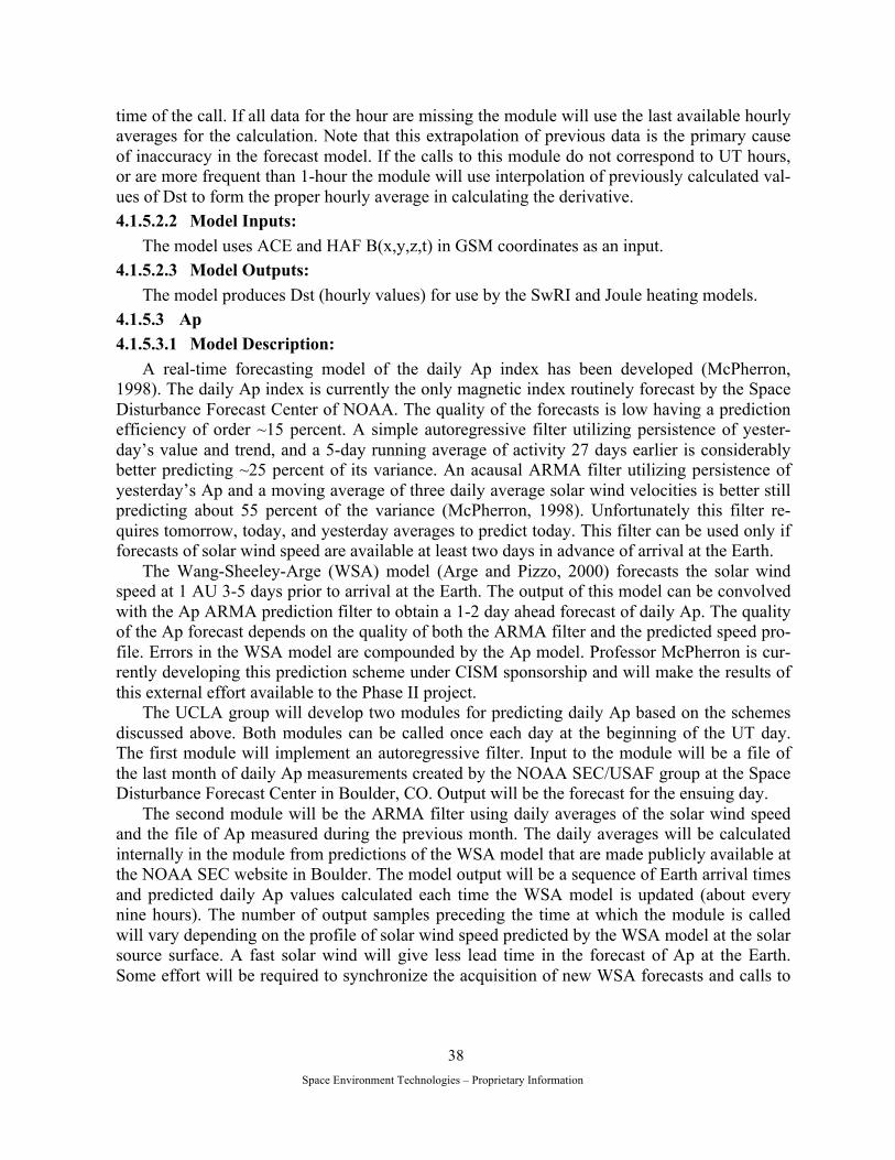
Space Environment Technologies – Proprietary Information
38
time of the call. If all data for the hour are missing the module will use the last available hourly averages for the calculation. Note that this extrapolation of previous data is the primary cause of inaccuracy in the forecast model. If the calls to this module do not correspond to UT hours, or are more frequent than 1-hour the module will use interpolation of previously calculated val-ues of Dst to form the proper hourly average in calculating the derivative. 4.1.5.2.2 Model Inputs:
The model uses ACE and HAF B(x,y,z,t) in GSM coordinates as an input. 4.1.5.2.3 Model Outputs:
The model produces Dst (hourly values) for use by the SwRI and Joule heating models. 4.1.5.3 Ap 4.1.5.3.1 Model Description:
A real-time forecasting model of the daily Ap index has been developed (McPherron, 1998). The daily Ap index is currently the only magnetic index routinely forecast by the Space Disturbance Forecast Center of NOAA. The quality of the forecasts is low having a prediction efficiency of order ~15 percent. A simple autoregressive filter utilizing persistence of yester-day’s value and trend, and a 5-day running average of activity 27 days earlier is considerably better predicting ~25 percent of its variance. An acausal ARMA filter utilizing persistence of yesterday’s Ap and a moving average of three daily average solar wind velocities is better still predicting about 55 percent of the variance (McPherron, 1998). Unfortunately this filter re-quires tomorrow, today, and yesterday averages to predict today. This filter can be used only if forecasts of solar wind speed are available at least two days in advance of arrival at the Earth.
The Wang-Sheeley-Arge (WSA) model (Arge and Pizzo, 2000) forecasts the solar wind speed at 1 AU 3-5 days prior to arrival at the Earth. The output of this model can be convolved with the Ap ARMA prediction filter to obtain a 1-2 day ahead forecast of daily Ap. The quality of the Ap forecast depends on the quality of both the ARMA filter and the predicted speed pro-file. Errors in the WSA model are compounded by the Ap model. Professor McPherron is cur-rently developing this prediction scheme under CISM sponsorship and will make the results of this external effort available to the Phase II project.
The UCLA group will develop two modules for predicting daily Ap based on the schemes discussed above. Both modules can be called once each day at the beginning of the UT day. The first module will implement an autoregressive filter. Input to the module will be a file of the last month of daily Ap measurements created by the NOAA SEC/USAF group at the Space Disturbance Forecast Center in Boulder, CO. Output will be the forecast for the ensuing day.
The second module will be the ARMA filter using daily averages of the solar wind speed and the file of Ap measured during the previous month. The daily averages will be calculated internally in the module from predictions of the WSA model that are made publicly available at the NOAA SEC website in Boulder. The model output will be a sequence of Earth arrival times and predicted daily Ap values calculated each time the WSA model is updated (about every nine hours). The number of output samples preceding the time at which the module is called will vary depending on the profile of solar wind speed predicted by the WSA model at the solar source surface. A fast solar wind will give less lead time in the forecast of Ap at the Earth. Some effort will be required to synchronize the acquisition of new WSA forecasts and calls to

Space Environment Technologies – Proprietary Information
39
this routine. 4.1.5.3.2 Model Inputs:
Input to the module will be a file of the last month of daily Ap measurements created by the NOAA SEC/USAF group at the Space Disturbance Forecast Center in Boulder, CO. HAF VSW are also available. 4.1.5.3.3 Model Outputs:
Output will be the Ap forecast for the ensuing day. 4.1.6 Neutral Thermosphere Winds 4.1.6.1 HWM93 4.1.6.1.1 Model Description:
The Horizontal Wind Model (1993) (Hedin et al., 1994, 1996) produces an empirical ther-mospheric wind velocity field. The following description comes from the HWM93 README file.
The HWM is an empirical model of the horizontal neutral wind in the upper thermosphere. It is based on wind data obtained from the AE-E and DE 2 satellites. A limited set of vector spherical harmonics is used to describe the zonal and meridional wind components. The first edition of the model released in 1987 (HWM87) was intended for winds above 220 km. With the inclusion of wind data from ground-based incoherent scatter radar and Fabry-Perot optical interferometers, HWM90 was extended down to 100 km and using MF/Meteor data HWM93 was extended down to the ground. Solar cycle variations are included (since HWM90), but they are found to be small and not always very clearly delineated by the current data. Variations with magnetic activity (Ap) are included. Mid- and low-latitude data are reproduced quite well by the model. The polar vortices are present, but not to full detail. The model describes the transition from predominately diurnal variations in the upper thermosphere to semidiurnal variations in the lower thermosphere and a transition from summer to winter flow above 140 km to winter to summer flow below. Significant altitude gradients in the wind extend up to 300 km at some local times. The model software is provided as one file HWM93.TXT; earlier ver-sions (HWM87, HWM90) are also available from NSSDC on request. The software provides zonal and meridional winds for specified latitude, longitude, time, and Ap index. 4.1.6.1.2 Model Inputs:
The model uses F10.7 and Ap as inputs. Time-resolved E10.7 is a probable replacement for F10.7. 4.1.6.1.3 Model Outputs:
The model produces neutral thermospheric horizontal winds, U(θ,φ,z,t), as an output for use in the GAIM model. 4.1.7 Neutral Thermosphere Densities 4.1.7.1 J70MOD 4.1.7.1.1 Model Description:
J70MOD computes thermospheric temperatures at all times, latitudes, longitudes, and 90–1500 km altitude with solar and geomagnetic inputs. It corrects two global temperature parame-

Space Environment Technologies – Proprietary Information
40
ters, i.e., the exospheric temperature, T∞ (600 km), and the inflection point temperature, TX (125 km). As in the Jacchia 1970 (J70) model, the local temperature profile, T(z), as a function of altitude, z, is uniquely determined by TX and T∞. The local values for TX and T∞ are both corrected indirectly through a global parameter known as the nighttime minimum exospheric temperature, TC, which is formed from solar driver inputs. This is used in J70 to describe the state of the entire thermosphere in response to solar extreme ultraviolet heating (Figure 13). 4.1.7.1.2 Model Inputs:
The model uses E10.7 or F10.7 and AP as inputs through the MFD file (Tobiska, 2003). In addition, the DCA delta-temperature spherical harmonic coefficients can be provided for more accurate regional mass densities and temperatures. 4.1.7.1.3 Model Outputs:
The model produces mass density, ρ(θ,φ,z,t), as an output. This is used to scale the NRLMSIS and the 1DTD neutral densities by first creating a mass density of the latter models’ outputs, then using the scaling ratios applied as a correction.
Figure 13. J70MOD Illustration of Spherical Harmonic Expansions for ΔTc and ΔTx (Degree = 3).

Space Environment Technologies – Proprietary Information
41
4.1.7.2 NRLMSIS00 4.1.7.2.1 Model Description:
MSIS86, MSISE90, NRLMSIS00 are provided in the public domain by work from A. He-din and co-workers, including M. Picone at NRL. The following text is from the MSISE90 Re-adme file.
The MSISE90 model describes the neutral temperature and densities in Earth's atmosphere from ground to thermospheric heights. Below 72.5 km the model is primarily based on the MAP Handbook (Labitzke) tabulation of zonal average temperature and pressure by Barnett and Corney, which was also used for the CIRA-86. Below 20 km these data were supplemented with averages from the National Meteorological Center (NMC). In addition, pitot tube, falling sphere, and grenade sounder rocket measurements from 1947 to 1972 were taken into consid-eration. Above 72.5 km MSISE-90 is essentially a revised MSIS-86 model taking into account data derived from space shuttle flights and newer incoherent scatter results. For someone inter-ested only in the thermosphere above 120 km, the author recommends the MSIS-86 model. MSISE is also not the model of preference for specialized tropospheric work but for studies that reach across several atmospheric boundaries.
The following text is from the NRLMSIS-00 Readme file. The NRLMSIS-00 empirical atmosphere model was developed by Mike Picone, Alan He-
din, and Doug Drob based on the MSISE90 model. The main differences to MSISE90 are noted in the comments at the top of the computer code. They involve: (1) the extensive use of drag and accelerometer data on total mass density; (2) the addition of a component to the total mass density that accounts for possibly significant contributions of O+ and hot oxygen at altitudes above 500 km; and (3) the inclusion of the SMM UV occultation data on [O2]. The MSISE90 model describes the neutral temperature and densities in Earth's atmosphere from ground to thermospheric heights. Below 72.5 km the model is primarily based on the MAP Handbook (Labitzke) tabulation of zonal average temperature and pressure by Barnett and Corney, which was also used for the CIRA-86. Below 20 km these data were supplemented with averages from the National Meteorological Center (NMC). In addition, pitot tube, falling sphere, and grenade sounder rocket measurements 1947–1972 were taken into consideration. Above 72.5 km MSISE-90 is essentially a revised MSIS-86 model using data derived from space shuttle flights and newer incoherent scatter results. For someone interested only in the thermosphere (above 120 km), the author recommends the MSIS-86 model. MSISE is also not the model of preference for specialized tropospheric work. It is rather for studies that reach across several atmospheric boundaries. 4.1.7.2.2 Model Inputs:
F10.7 and Ap are the nominal inputs into MSIS-type models. Time-resolved E10.7 can re-place F10.7. 4.1.7.2.3 Model Outputs:
Neutral densities N(θ,φ,z,t) of O, O2, N2, H, He, N, and temperature (T) are provided either as is or scaled using J70MOD mass densities, for use in the GAIM model.
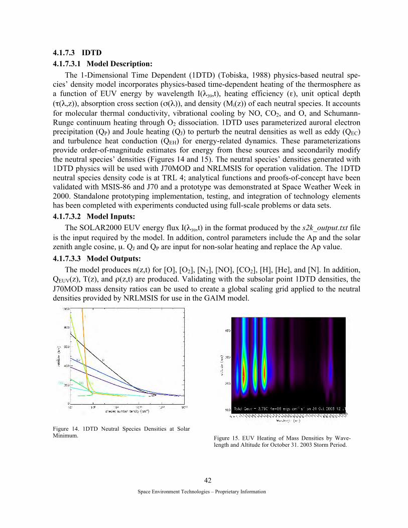
Space Environment Technologies – Proprietary Information
42
4.1.7.3 IDTD 4.1.7.3.1 Model Description:
The 1-Dimensional Time Dependent (1DTD) (Tobiska, 1988) physics-based neutral spe-cies’ density model incorporates physics-based time-dependent heating of the thermosphere as a function of EUV energy by wavelength I(λ39,t), heating efficiency (ε), unit optical depth (τ(λ,z)), absorption cross section (σ(λ)), and density (Mi(z)) of each neutral species. It accounts for molecular thermal conductivity, vibrational cooling by NO, CO2, and O, and Schumann-Runge continuum heating through O2 dissociation. 1DTD uses parameterized auroral electron precipitation (QP) and Joule heating (QJ) to perturb the neutral densities as well as eddy (QEC) and turbulence heat conduction (QEH) for energy-related dynamics. These parameterizations provide order-of-magnitude estimates for energy from these sources and secondarily modify the neutral species’ densities (Figures 14 and 15). The neutral species’ densities generated with 1DTD physics will be used with J70MOD and NRLMSIS for operation validation. The 1DTD neutral species density code is at TRL 4; analytical functions and proofs-of-concept have been validated with MSIS-86 and J70 and a prototype was demonstrated at Space Weather Week in 2000. Standalone prototyping implementation, testing, and integration of technology elements has been completed with experiments conducted using full-scale problems or data sets. 4.1.7.3.2 Model Inputs:
The SOLAR2000 EUV energy flux I(λ39,t) in the format produced by the s2k_output.txt file is the input required by the model. In addition, control parameters include the Ap and the solar zenith angle cosine, µ. QJ and QP are input for non-solar heating and replace the Ap value. 4.1.7.3.3 Model Outputs:
The model produces n(z,t) for [O], [O2], [N2], [NO], [CO2], [H], [He], and [N]. In addition, QEUV(z), T(z), and ρ(z,t) are produced. Validating with the subsolar point 1DTD densities, the J70MOD mass density ratios can be used to create a global scaling grid applied to the neutral densities provided by NRLMSIS for use in the GAIM model.
Figure 14. 1DTD Neutral Species Densities at Solar Minimum.
Figure 15. EUV Heating of Mass Densities by Wave-length and Altitude for October 31. 2003 Storm Period.

Space Environment Technologies – Proprietary Information
43
4.1.8 Solar Irradiances 4.1.8.1 SOLAR2000 4.1.8.1.1 Model Description:
The SOLAR2000 (Tobiska et al., 2000) Operational Grade (OP) model {S2KOP V2.22 (FGen 2/D1.4)} provides 1 AU adjusted or observed daily historical, nowcast, and forecast so-lar irradiance products (Figure 16). The OP model is run every hour on the SET proprietary server which also generates high time resolution irradiance forecast products such as the I(λ39,t) spectral solar irradiances as well as the integrated irradiance proxy (E10.7) daily values. The high time resolution data is provided in 3-hour time bins that correspond to the 0, 3, 6, 9, 12, 15, 18, and 21 UT releases of the ap index and is updated once per hour. When the GOES-N data from the five EUV broadband detectors comes on-line (2006), the time resolution will be every 5 minutes which captures solar X-ray and EUV flare evolution. The high time resolution forecast is made out to 72 hours. The OP model provides data on demand (24/7) via a user ac-count on a secure server. A typical file that is produced for the high time resolution data is the Modified Flux Data (MFD) bulletin (Tobiska, 2003) that provides the previous 48-hours of is-sued data and nowcast data as well as the 72-hour forecast data. The file contains a fixed-length metadata section describing the file name, the issued date and time (UT), the manufacturer and contact information, the units used for the file data, the data source and production location, and the missing data flag designator symbol. Parameters provided in this file are one line for each time record in column format that include time (UT time in YYYYMMDDhhmm format), S_C, F10, F81, LYA, L81, E10, E81, A_p, E3h, B3h, a3h, E1s, a1s, and SRC. 4.1.8.1.2 Model Inputs:
The model uses F10.7 and Mg II cwr as inputs. In the future, it will use NOAA GOES-N as an input.
Figure 16. Forecast Coronal and Chromospheric Proxies on Multiple Time Scales that Drive SOLAR2000.
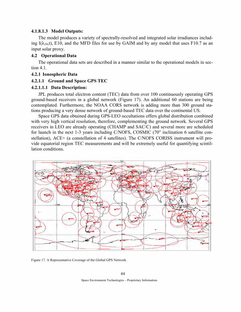
Space Environment Technologies – Proprietary Information
44
4.1.8.1.3 Model Outputs: The model produces a variety of spectrally-resolved and integrated solar irradiances includ-
ing I(λ39,t), E10, and the MFD files for use by GAIM and by any model that uses F10.7 as an input solar proxy. 4.2 Operational Data
The operational data sets are described in a manner similar to the operational models in sec-tion 4.1. 4.2.1 Ionospheric Data 4.2.1.1 Ground and Space GPS TEC 4.2.1.1.1 Data Description:
JPL produces total electron content (TEC) data from over 100 continuously operating GPS ground-based receivers in a global network (Figure 17). An additional 60 stations are being contemplated. Furthermore, the NOAA CORS network is adding more than 300 ground sta-tions producing a very dense network of ground-based TEC data over the continental US.
Space GPS data obtained during GPS-LEO occultations offers global distribution combined with very high vertical resolution, therefore, complementing the ground network. Several GPS receivers in LEO are already operating (CHAMP and SAC/C) and several more are scheduled for launch in the next 1-3 years including C/NOFS, COSMIC (70° inclination 6 satellite con-stellation), ACE+ (a constellation of 4 satellites). The C/NOFS CORISS instrument will pro-vide equatorial region TEC measurements and will be extremely useful for quantifying scintil-lation conditions.
Figure 17. A Representative Coverage of the Global GPS Network.

Space Environment Technologies – Proprietary Information
45
4.2.1.1.2 Data Inputs: The TEC measurements include JPL (global ground GPS), NOAA CORS (CONUS ground
GPS), C/NOFS CORISS (equatorial satellite GPS), and eventual COSMIC (equatorial and mid-latitude satellite GPS) as well as SBIRS Lo (global satellite GPS). These are slant path TEC. 4.2.1.1.3 Data Outputs:
The TEC measurements include JPL (global ground GPS), NOAA CORS (CONUS ground GPS), CHAMP, SAC/C, C/NOFS, and COSMIC. All data correspond to line-of-sight cali-brated and absolute TEC measurements with a 0.1 TECU precision and 1-2 TECU accuracy. In addition, TEC data from LEO antennas looking upward (primarily used for navigation pur-poses) will be input into GAIM providing a strong constraint on the topside ionosphere and plasmasphere. 4.2.1.2 ne 4.2.1.2.1 Data Description:
Electron density profiles are provided by latitude, longitude, altitude, and time. 4.2.1.2.2 Data Inputs:
Multiple inputs into GAIM are used. 4.2.1.2.3 Data Outputs:
ne(θ,φ,z,t) is produced by GAIM. 4.2.1.3 Te and Ti (temperatures) 4.2.1.3.1 Data Description:
Electron and ion temperature empirical models are embedded inside the GAIM model. 4.2.1.3.2 Data Inputs:
Multiple inputs into GAIM are used. 4.2.1.3.3 Data Outputs:
Te, Ti are produced by GAIM. 4.2.1.4 UV (SSULI) 4.2.1.4.1 Data Description:
The SSULI UV instrument on a DMSP satellite will produce maps of altitude-resolved air-glow from O/N2 observations. Variations in this ratio are indicative of energy deposition. Fidel-ity of the airglow measurements can be validated with a derived effective 1-40 nm EUV flux (Qeuv) (Tobiska, 2002) that would be required to produce the observed airglow and SO-LAR2000 produces an integrated 1-40 nm EUV energy flux time series (E1_40) that will be used in validation. 4.2.1.4.2 Data Inputs:
SSULI UV airglow measurements are processed. In addition, an effective EUV flux will be produced and will be compared to E1_40 as a data validation. 4.2.1.4.3 Data Outputs:
The UV data is assimilated in the GAIM model.
Space Environment Technologies – Proprietary Information
46
4.2.2 Solar Wind 4.2.2.1 IMF B 4.2.2.1.1 Data Description:
Solar wind magnetic field magnitude and direction are available from the ACE spacecraft and HAF model. 4.2.2.1.2 Data Inputs:
Magnetograms and optical observations are input into HAF. 4.2.2.1.3 Data Outputs:
B(x,y,z,t) as produced by either ACE or HAF. 4.2.2.2 Photospheric Magnetogram 4.2.2.2.1 Data Description:
Photospheric magnetograms of the solar magnetic field source surface are primary data that provide information about the polarity of the solar photospheric magnetic field. They can be translated, through models, into current sheet specification and, in turn, characteristics of the solar wind. 4.2.2.2.2 Data Inputs:
NSO observations. 4.2.2.2.3 Data Outputs:
Photospheric magnetograms are used by HAF. 4.2.2.3 VSW 4.2.2.3.1 Data Description:
Solar wind velocity is produced by the ACE spacecraft and by the HAF model. 4.2.2.3.2 Data Inputs:
ACE makes measurements and HAF uses magnetograms. 4.2.2.3.3 Data Outputs:
VSW are produced by ACE and HAF. 4.2.3 Plasma Drifts 4.2.3.1 w 4.2.3.1.1 Data Description:
Plasma drift velocity magnitudes are specified by latitude, longitude, altitude, and time. They are produced by the DICM, HM87, W95, and SF99 models as well as measured by DMSP UVI and C/NOFS VERI instruments for use in GAIM. 4.2.3.1.2 Data Inputs:
ACE and HAF IMF B are used to produce modeled plasma drift velocities at high latitudes while E10.7 and/or F10.7 are used for low latitudes. 4.2.3.1.3 Data Outputs:
w(θ,φ,z,t) is used in GAIM.

Space Environment Technologies – Proprietary Information
47
4.2.4 Particle Precipitation 4.2.4.1 Kp 4.2.4.1.1 Data Description:
Kp is a 3-hourly geomagnetic index provided though NOAA SEC. 4.2.4.1.2 Data Inputs:
Observing stations. 4.2.4.1.3 Data Outputs:
Kp is used in the SwRI model. SET provides a forecast conversion of 3-hourly Kp values to ap. 4.2.4.2 F 4.2.4.2.1 Data Description:
Low- and high-energy particle precipitation, F(θ,φ,t), contributes energy to the polar re-gions. We use two methods to ensure a transition from climatology to weather. First, the 1DTD model and GAIM both use parameterization of particle precipitation to achieve proper scales of energy input from this source. Second, a statistical, climatological model of electron precipita-tion that is very convenient for operations has been compiled from the NOAA-12 data by re-searchers at SwRI (Wüest et al., 2002).
The following text comes from the NOAA SEC web site description. The Space Environment Monitor (SEM) that is regularly flown on the NOAA POES (for-
merly TIROS) series of low-altitude (850 km), polar-orbiting (98 degree inclination) spacecraft contains two sets of instruments that monitor the energetic charged-particle environment near Earth. An upgraded SEM, called SEM-2, began operations with the launch of NOAA-15 and is currently the prime source of observations.
The Total Energy Detector (TED) in SEM-2 provides the data used to determine the level of auroral activity and generate the statistical maps presented on NOAA SEC’s ‘POES Auroral Activity’ website. This instrument monitors the energy fluxes carried into the atmosphere by electrons and positive ions over the energy range between 50 and 20,000 electron Volts (eV). Particles of these energies are stopped by the atmosphere of the Earth at altitudes above 100 km, producing aurora. The instrument design utilizes cylindrical, curved-plate electrostatic ana-lyzers to select (by impressing a variable voltage between the analyzer plates) the species and energy of those particles that are permitted to reach the detector. Those particles that pass through the analyzer are counted, one by one, by the detector (a Channeltron open-windowed electron multiplier). Eight such detector systems are included in the SEM, four to monitor posi-tive ions and four to monitor electrons. They are mounted in groups of four, one group viewing radially outward from Earth and the other viewing at 30 degrees to the first. Whenever the sat-ellite is poleward of a geographic latitude of about 30 degrees, all eight detectors view the charged particles that will be guided by the geomagnetic field into the atmosphere below the satellite. A satellite data processing unit converts the Channeltron responses to measures of in-tegrated power flux; these are telemetered to the ground along with crude information about the energy distribution of the electrons and positive ions. Data processing on the ground combines observations from the eight instruments to obtain the total power flux carried into the atmos-phere by these particles.

Space Environment Technologies – Proprietary Information
48
The second instrument in the second-generation SEM-2 is the Medium Energy Proton and Electron Detector (MEPED) which provides the measurements used to create the plots on NOAA SEC’s ‘POES Energetic Particles’ website. This instrument includes four solid-state detector telescopes, two to measure the intensity of electrons between 30 and 1000 keV and two to measure the intensity of protons (positive ions) between 30 and 6900 keV, as well as solid-state “dome” detectors that measure the intensities of protons 16 – 275 MeV.
The solid-state detector telescopes are mounted in pairs. One pair views radially outward from Earth to monitor particles that will enter the atmosphere in the polar regions; the other pair is mounted at nearly 90 degrees to the first to view charged particles that will “magneti-cally mirror” near the satellite. The field of view of each detector system is only 30 degrees so that the angular distribution of the particles may be determined. These detectors are designed to monitor the intensities of energetic particles in Earth's radiation belts and during solar particle events.
In addition, the MEPED contains “dome” detectors with very large fields of view (nearly 180 degrees) and are mounted on the side of the spacecraft facing away from Earth to monitor particles incident upon the atmosphere. These detectors are designed to detect and monitor en-ergetic solar particles that cause severe ionospheric disturbances during solar particle events. 4.2.4.2.2 Data Inputs:
Dst, PC, Kp, F10.7 and E10.7 are inputs for the SwRI model; POES Pe, Pp measurements come from NOAA. 4.2.4.2.3 Data Outputs:
F(θ,φ,t) is used by the GAIM model. 4.2.4.3 Pe, Pp, and Qp 4.2.4.3.1 Data Description:
Instruments on board the Polar-orbiting Operational Environmental Satellite (POES) con-tinually monitor the protons and electrons power flux. Fuller-Rowell and Evans (1987) devel-oped a technique that uses the power flux observations obtained during a single pass of the sat-ellite over a polar region (which takes about 25 minutes) to estimate the total power deposited in an entire polar region by the 50 eV to 20 keV particles. Relationship to particle heating global value must still be understood and is a possible Phase III activity. 4.2.4.3.2 Data Inputs:
POES measurements. 4.2.4.3.3 Data Outputs:
Pe (electron precipitation power) and Pp (proton precipitation power) are used by the GAIM model. 4.2.5 High Latitude Heating 4.2.5.1 Ap 4.2.5.1.1 Data Description:
Ap is a daily planetary geomagnetic index provided though NOAA SEC and ap is the 3-hourly index.
Space Environment Technologies – Proprietary Information
49
4.2.5.1.2 Data Inputs: The McPherron model (1998) uses historical Ap files and VSW.
4.2.5.1.3 Data Outputs: Daily Ap from the McPherron ARMA model algorithm with transform to 3-hourly using
Kp scaling from USAF. As part of the translation of daily Ap to 3-hourly ap forecasts, SET will use a conversion algorithm that can unit scale daily Ap relative to the USAF forecast 3-hourly Kp values. 4.2.5.2 QJ 4.2.5.2.1 Data Description:
Joule heating is a derived quantity produced by the Knipp model. It is used by the 1DTD model. 4.2.5.2.2 Data Inputs:
Dst and PC are the Knipp model inputs. 4.2.5.2.3 Data Outputs:
QJ is used by the 1DTD model. 4.2.5.3 Dst 4.2.5.3.1 Data Description:
The Disturbance Storm Time (Dst) index can be thought of as a proxy for the electrical in-teraction of the nightside magnetosphere and ionosphere. Kyoto provides the near real-time data stream while predictions are made by UCLA and other groups. 4.2.5.3.2 Data Inputs:
Kyoto provides the near real-time data stream while predictions are made by UCLA and other groups. 4.2.5.3.3 Data Outputs:
Hourly Dst from the UCLA prediction method. 4.2.5.4 PC 4.2.5.4.1 Data Description:
The PC-index, a proxy for the electric field imposed on the polar ionosphere by the solar wind, is based on an idea by Troshichev and developed in papers including Troshichev et al. 1988. It is based on an assembled a set of 12,000 hemispherically integrated Joule heating val-ues derived from the Assimilative Mapping of Ionospheric Electrodynamics (AMIE) mapping procedure (Richmond and Kamide, 1988) as a statistical ensemble for binning Joule power against geomagnetic activity. The procedure may underestimate Joule heating during strong storms. The data from 1975 – 1993 are published in Report UAG-103 and monthly Thule plots appear in SGD since October 1993.
An additional description comes from the NOAA SGD Explanation of Data Reports. The Geomagnetic Polar Cap (PC) Index (PC) is an index for magnetic activity in the (P)olar (C)ap. It is based on data from a single near-pole station, and aimed to monitor the polar cap magnetic activity generated by such solar wind parameters as the southward component of the interplane-tary magnetic field (IMF), the azimuthal component of the IMF B(y), and the solar wind veloc-
Space Environment Technologies – Proprietary Information
50
ity, v. The station Thule, located in the village Qaanaaq in Greenland at 86.5 geomagnetic in-variant latitude, fulfills the requirement of being close to the magnetic pole in the northern hemisphere. The station Vostok at 83.3 does the same in the southern hemisphere. The PC in-dex is derived independently for these two stations. The northern index is most commonly used and work continues in the scientific community to reconcile the northern and southern indices. Currently, the northern polar cap index is available only at the end of the UT day. The southern PC index has been available every 15 minutes but the station producing the Index, Vostok, may be closed. 4.2.5.4.2 Data Inputs:
Magnetic field measurements. 4.2.5.4.3 Data Outputs:
PC is used in the SwRI and Joule heating models. 4.2.6 Neutral Thermosphere Winds 4.2.6.1 U 4.2.6.1.1 Data Description:
Horizontal (meridional and zonal) wind magnitude by latitude, longitude, altitude, and time are produced by the HWM93 model. 4.2.6.1.2 Data Inputs:
F10.7, E10.7, and Ap. 4.2.6.1.3 Data Outputs:
U(θ,φ,z,t) is used by the GAIM model. 4.2.7 Neutral Thermosphere Densities 4.2.7.1 DCA 4.2.7.1.1 Data Description:
The DCA model was developed to operational status through the USAF HASDM project and is described in an AIAA abstract by Stephen J. Casali and William N. Barker, “Dynamic Calibration Atmosphere (DCA) For The High Accuracy Satellite Drag Model (HASDM),” (2002):
“The Dynamic Calibration Atmosphere (DCA) represents Phase I of the High Accuracy Satellite Drag Model (HASDM) initiative. DCA uses tracking data on a set of calibration satel-lites to determine corrections to the Jacchia 70 density model in near real-time. The density cor-rections take the form of spherical harmonic expansions of two Jacchia temperature parameters that enhance spatial resolution. [Their paper] describes the DCA solution over the first half of 2001 and its application to forty evaluation satellites. Improvements due to DCA in ballistic coefficient consistency, epoch accuracy, and epoch covariance realism are measured and dem-onstrated.”
U.S. Space Command is in the final stages of placing the DCA algorithm into operations at TRL 9 as it has gone through extensive development, testing, validation, and implementation during 2001-2004. The system delivery is in progress and data are anticipated from this system by 2005. We note that these data are not available to the community outside of Space Com-

Space Environment Technologies – Proprietary Information
51
mand in real-time. An agreement would be required between DoD agencies to permit use of the DCA coefficients in an AFWA rack-mount system of this design. The prototype system we are designing runs in the lower accuracy mode with only the J70MOD. The high accuracy capabil-ity with the inclusion of DCA coefficients would be a Phase III enhancement activity. 4.2.7.1.2 Data Inputs:
The model uses Space Surveillance Network (SSN) real-time data. SSN data is the compos-ite data set of all NORAD tracked objects and their Two-Line Elements (TLE). 4.2.7.1.3 Data Outputs:
The model produces a delta-temperature coefficient file (spherical harmonic) for inclusion into the J70MOD model to correct the climatological values for the current epoch or forecast out to 72 hours. 4.2.7.2 ρ 4.2.7.2.1 Data Description:
Thermospheric mass density by latitude, longitude, altitude, and time are produced by the J70MOD model or, in altitude and time, by the 1DTD model. 4.2.7.2.2 Data Inputs:
E10.7, Ap, and I(λ39,t) are inputs. 4.2.7.2.3 Data Outputs:
ρ(θ,φ,z,t) is used in a scaling array as a correction term for the NRLMSIS mass densities then neutral densities; it will be validated by 1DTD. 4.2.7.3 N 4.2.7.3.1 Data Description:
Neutral thermospheric densities by species and altitude, latitude, longitude, and time are provided by NRLMSIS and 1DTD. These are climatological values and must be transformed to mass densities, then corrected at the current epoch by J70MOD mass densities, and retrans-formed back to neutral densities. 4.2.7.3.2 Data Inputs:
E10.7, F10.7, Ap, and I(λ39,t) are inputs. 4.2.7.3.3 Data Outputs:
N(θ,φ,z,t) is used by the GAIM model. 4.2.8 Solar Irradiances 4.2.8.1 EM Observations 4.2.8.1.1 Data Description:
Electromagnetic field observations (EM obs) are solar X-ray, optical, and radio emission observations that provide information related to Coronal Mass Ejections (CMEs) and are moni-tored by ground observatories (National Solar Observatory) or by spacecraft (GOES SXI, YOHKOH, SOHO).

Space Environment Technologies – Proprietary Information
52
4.2.8.1.2 Data Inputs: Observations.
4.2.8.1.3 Data Outputs: X-ray, visible, and radio emissions are used by the HAF model.
4.2.8.2 F10.7 4.2.8.2.1 Data Description:
F10.7 is the daily value of the 10.7-cm solar radio emission measured by the Canadian Na-tional Research Council Dominion Radio Astrophysical Observatory at Penticton, BC, Canada. The “observed” value is the number measured by the solar radio telescope at the observatory, is modulated by the level of solar activity and the changing distance between the Earth and Sun, and is the quantity to use when terrestrial phenomena are being studied. When the Sun is being studied, it is useful to remove the annual modulation of F10 by the changing Earth-Sun distance and the “1 AU adjusted” value is corrected for variations in the Earth-Sun distance, giving the average distance. Penticton measures the F10, NOAA SEC reports the F10, and numerous or-ganizations, including SET, forecast the F10. Its units are solar flux units (sfu) or 1×10-22 Watts per meter squared per Hertz. Normal practice is to refer to the value as “F10.7” but F10 is often used here as an abbreviation. 4.2.8.2.2 Data Inputs:
Observations. 4.2.8.2.3 Data Outputs:
F10.7 is used in multiple models as a solar energy input. 4.2.8.3 Mg II cwr 4.2.8.3.1 Data Description:
The Mg II core-to-wing ratio (cwr) data is available on a daily basis from the NOAA Space Environment Center (SEC) (Viereck et al., 2001). It is the h and k line emission from Mg II and found in the 280 nm absorption feature of the solar spectrum. The ratio of the h and k line variation to the continuum emission at the wings of the absorption feature provides an excellent and highly precise method of determining solar chromospheric irradiance (full-disk) variability. We note that the solar EUV emission responsible for the formation of the ionosphere and heat-ing of the neutral thermosphere comes primarily from the same solar temperature region (chromosphere) as the Mg II emission and this is why it is such a good proxy. 4.2.8.3.2 Data Inputs:
NOAA-16 SBUV Mg II core-to-wing ratio data is provided operationally at 0720 UT daily. The NOAA-17 SBUV Mg II cwr data is operational and being validated at NOAA SEC at 12 hours offset to the NOAA-16 data. 4.2.8.3.3 Data Outputs:
Community project (NOAA-coordinated by R. Viereck) Mg II cwr daily values are opera-tionally used by the SOLAR2000 model.
Space Environment Technologies – Proprietary Information
53
4.2.8.4 GOES-N 4.2.8.4.1 Data Description:
The GOES-N EUV broadband data will become available through NOAA SEC in 2005-2006. There are five broadband EUV sensors in the instrument package and these data will be translated into an EUV solar spectrum with up to 5-minute time resolution which is beneficial for real-time solar EUV flare monitoring. 4.2.8.4.2 Data Inputs:
Measurements. 4.2.8.4.3 Data Outputs:
GOES-N EUV will be used by SOLAR2000 to produce spectral and integrated EUV irradi-ances. 4.2.8.5 I 4.2.8.5.1 Data Description:
I(λ39,t) is the daily value of the solar EUV spectral irradiances in 39 wavelength groups and lines. In this project they are reported as photon or energy flux. 4.2.8.5.2 Data Inputs:
F10.7 and Mg II cwr are currently used to derive the irradiances, then GOES-N EUV data after 2005. 4.2.8.5.3 Data Outputs:
I(λ39,t) is used by the GAIM model. 4.2.8.6 E10.7 4.2.8.6.1 Data Description:
Solar EUV energy flux between 1-105 nm is integrated, regressed with F10.7 over 3 solar cycles, and reported in F10.7 solar flux units (sfu) (Tobiska, 2001). This proxy is generated by the SOLAR2000 model and reports the same energy content as the full solar irradiance spec-trum used by physics-based models. 4.2.8.6.2 Data Inputs:
F10.7, Mg II, and GOES-N are inputs. 4.2.8.6.3 Data Outputs:
E10.7 is used as a high time resolution substitute for F10.7 in operational models. There has been ongoing research over the past four years that has validated and verified the use of E10 in place of F10. In most daily applications, E10 and F10 perform nearly the same although most applications are derived using F10.7. However, the advantage of E10.7 is that time resolution and consistency with actual solar irradiances is obtained and this advantage is used in our pro-ject. All modules that normally use F10.7 will still be able to use that parameter; part of the validation work in Phase II will be to ensure that E10.7 provides an operational advantage. Where this is not the case, F10.7 will be used.

Space Environment Technologies – Proprietary Information
54
4.3 Operational Forecast System 4.3.1 System Concept of Operations
There are two architecture approaches that are being developed for this operational iono-spheric forecast system. One is primary and one is secondary. These approaches have emerged from a Unified Modeling Language (UML) “use-case” point of view which is described in more detail below as related to this project; the approaches also derive from the SET process for developing operational systems life cycles. Figure 18 graphically shows our two ap-proaches.
The primary approach is a distributed network based upon an Operational Database Man-agement System (ODBMS) architecture. The key elements are: (1) an input data stream from third parties; (2) a client server that handles asynchronous file exchanges between geographi-cally separated models hosted on separated prime and backup computers; (3) a real-time reposi-tory database for dynamic data sets; and (4) a customer server interface for access to real-time and forecast ionospheric parameters. Strengths include fault-tolerance and system flexibility for prototype development. Risks include susceptibility to network disruptions and management complexity for distributed systems.
The secondary approach is a rack-mount, clustered turn-key system based upon a central server and database at one physical location that runs continuously and is linked to other local computers where all models reside. The server/database system’s software languages and data interface routines collect the proper input data sets that are needed to provide real-time and forecast ionospheric parameters. The strengths of this system include information security and control at a single site. Risks include limitations to system upgrades and susceptibility to envi-ronment failures at the location of the rack-mount/turn-key system.
Figure 18. Two Approaches to the Concept of Operations Using a Distributed Network and a Rack-Mount/Turn-Key System.
Space Environment Technologies – Proprietary Information
55
This report describes the distributed network system since it contains all components that are required by the rack-mount/turn-key system. Once a distributed network is functional, the porting of models, server, and database functions to a rack-mount “system-in-a-box” is rela-tively straightforward. The rack-mount system can be considered a derivative of the distributed network.
Recalling the top level geophysical information flow shown in Figure 1, the data and model linkages shown in Figure 2 as a function of discipline area, data source, model host institution, and input/output data designation, and the data streams shown in Figure 4, we now describe the concept of operations that ties this architecture together.
…run models asynchronously, linked through dynamic data input and output The raw operational input data is collected from third parties by a client server located at
Space Environment Technologies (SET). The server’s software (described in section 4.3.2.3) creates metadata tags for all data objects and deposits the data object combined with its meta-data as a “data suitcase” into the dynamic section of the database for use by models or users. Models, running at their appropriate geophysical cadences, are developed and hosted at SET and at partner institutions including USC (and their partner, JPL), EXPI, and SwRI. Requests for data inputs by models are made to the client server which then extracts and forwards the requested past, present, or future data suitcase to the requestor. Outputs from the models are collected by the client server and stored in the dynamic database for use by other models.
Customers will access the data products by making requests to the server using either op-erational application software for automated server connections, a capability SET now provides for its SOLAR2000 Professional Grade model, or browsers for manual, interactive sessions. For example, a customer may want electron densities for a particular time, latitude, longitude and the information content of these data objects would be provided “just-in-time.” The use of dynamic metadata allows traceability for all I/O requests from models, customers, or users.
From a first look at Figures 1 and 2, it is apparent there would be an unmanageable risk if one were to try running the models in a synchronized, end-to-end manner. There are numerous potential single points of failure which could lead to system execution times longer than the anticipated cadence. In addition, with synchronized runs, there is a susceptibility to catastrophic failure in the event of component failure. We have avoided this risk by incorporating a key de-sign philosophy: models are run asynchronously and linked through dynamic data input and output. 4.3.1.1 Functional System Design
… component failures and data communication interrupts do not produce cata-strophic failure. Using the philosophy of asynchronously linked models within a dynamic data flow, our
software architecture embodies an additional guiding concept: produce accurate real-time and forecast ionospheric parameters while maintaining output data integrity even with component failures and data dropouts or latency. A corollary design practice is used: no single points of failure, data dropouts or latency will stop the operational generation of real-time and forecast ionospheric information. This guidance implies that component failures, data dropouts, and data latency are identified, reported, and corrected where necessary such that the largest risk for
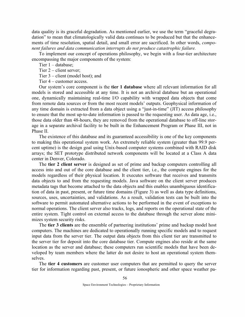
Space Environment Technologies – Proprietary Information
56
data quality is its graceful degradation. As mentioned earlier, we use the term “graceful degra-dation” to mean that climatologically valid data continues to be produced but that the enhance-ments of time resolution, spatial detail, and small error are sacrificed. In other words, compo-nent failures and data communication interrupts do not produce catastrophic failure.
To implement our concept of operations philosophy, we begin with a four-tier architecture encompassing the major components of the system:
Tier 1 – database; Tier 2 – client server; Tier 3 – client (model host); and Tier 4 – customer access. Our system’s core component is the tier 1 database where all relevant information for all
models is stored and accessible at any time. It is not an archival database but an operational one, dynamically maintaining real-time I/O capability with wrapped data objects that come from remote data sources or from the most recent models’ outputs. Geophysical information of any time domain is extracted from a data object using a “just-in-time” (JIT) access philosophy to ensure that the most up-to-date information is passed to the requesting user. As data age, i.e., those data older than 48-hours, they are removed from the operational database to off-line stor-age in a separate archival facility to be built in the Enhancement Program or Phase III, not in Phase II.
The existence of this database and its guaranteed accessibility is one of the key components to making this operational system work. An extremely reliable system (greater than 99.9 per-cent uptime) is the design goal using Unix-based computer systems combined with RAID disk arrays; the SET prototype distributed network components will be located at a Class A data center in Denver, Colorado.
The tier 2 client server is designed as set of prime and backup computers controlling all access into and out of the core database and the client tier, i.e., the compute engines for the models regardless of their physical location. It executes software that receives and transmits data objects to and from the requesting models. Java software on the client server produces metadata tags that become attached to the data objects and this enables unambiguous identifica-tion of data in past, present, or future time domains (Figure 3) as well as data type definitions, sources, uses, uncertainties, and validations. As a result, validation tests can be built into the software to permit automated alternative actions to be performed in the event of exceptions to normal operations. The client server also tracks, logs, and reports on the operational state of the entire system. Tight control on external access to the database through the server alone mini-mizes system security risks.
The tier 3 clients are the ensemble of partnering institutions’ prime and backup model host computers. The machines are dedicated to operationally running specific models and to request input data from the server tier. The output data objects from this client tier are transmitted to the server tier for deposit into the core database tier. Compute engines also reside at the same location as the server and database; these computers run scientific models that have been de-veloped by team members where the latter do not desire to host an operational system them-selves.
The tier 4 customers are customer user computers that are permitted to query the server tier for information regarding past, present, or future ionospheric and other space weather pa-
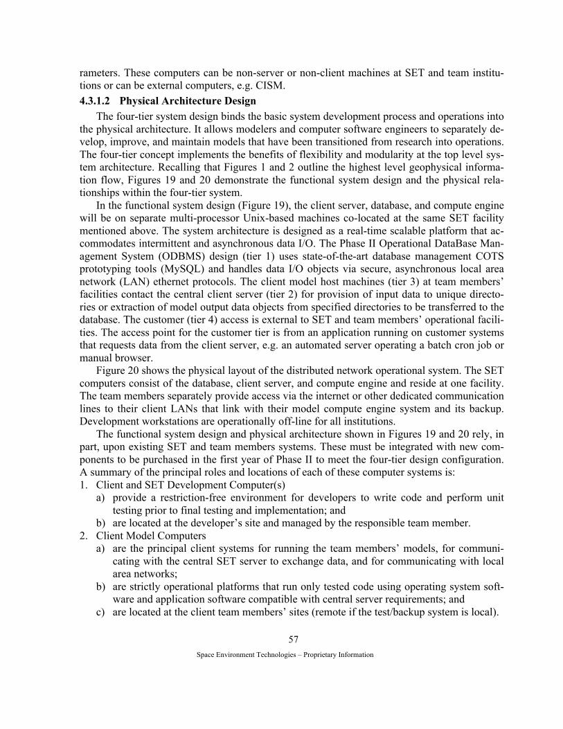
Space Environment Technologies – Proprietary Information
57
rameters. These computers can be non-server or non-client machines at SET and team institu-tions or can be external computers, e.g. CISM. 4.3.1.2 Physical Architecture Design
The four-tier system design binds the basic system development process and operations into the physical architecture. It allows modelers and computer software engineers to separately de-velop, improve, and maintain models that have been transitioned from research into operations. The four-tier concept implements the benefits of flexibility and modularity at the top level sys-tem architecture. Recalling that Figures 1 and 2 outline the highest level geophysical informa-tion flow, Figures 19 and 20 demonstrate the functional system design and the physical rela-tionships within the four-tier system.
In the functional system design (Figure 19), the client server, database, and compute engine will be on separate multi-processor Unix-based machines co-located at the same SET facility mentioned above. The system architecture is designed as a real-time scalable platform that ac-commodates intermittent and asynchronous data I/O. The Phase II Operational DataBase Man-agement System (ODBMS) design (tier 1) uses state-of-the-art database management COTS prototyping tools (MySQL) and handles data I/O objects via secure, asynchronous local area network (LAN) ethernet protocols. The client model host machines (tier 3) at team members’ facilities contact the central client server (tier 2) for provision of input data to unique directo-ries or extraction of model output data objects from specified directories to be transferred to the database. The customer (tier 4) access is external to SET and team members’ operational facili-ties. The access point for the customer tier is from an application running on customer systems that requests data from the client server, e.g. an automated server operating a batch cron job or manual browser.
Figure 20 shows the physical layout of the distributed network operational system. The SET computers consist of the database, client server, and compute engine and reside at one facility. The team members separately provide access via the internet or other dedicated communication lines to their client LANs that link with their model compute engine system and its backup. Development workstations are operationally off-line for all institutions.
The functional system design and physical architecture shown in Figures 19 and 20 rely, in part, upon existing SET and team members systems. These must be integrated with new com-ponents to be purchased in the first year of Phase II to meet the four-tier design configuration. A summary of the principal roles and locations of each of these computer systems is: 1. Client and SET Development Computer(s)
a) provide a restriction-free environment for developers to write code and perform unit testing prior to final testing and implementation; and
b) are located at the developer’s site and managed by the responsible team member. 2. Client Model Computers
a) are the principal client systems for running the team members’ models, for communi-cating with the central SET server to exchange data, and for communicating with local area networks;
b) are strictly operational platforms that run only tested code using operating system soft-ware and application software compatible with central server requirements; and
c) are located at the client team members’ sites (remote if the test/backup system is local).

Space Environment Technologies – Proprietary Information
58
Figure 19. Data and Models at Host Institutions are Linked With a Client Server and Database in a Distributed Network in This Functional System Design.
Figure 20. The SET Client Servers (Both Primary and Backup), The DBMS, and Compute Engine are Shown in Physical Rela-tionship to Client Host Machines, e.g., USC/JPL, SwRI, and EXPI.
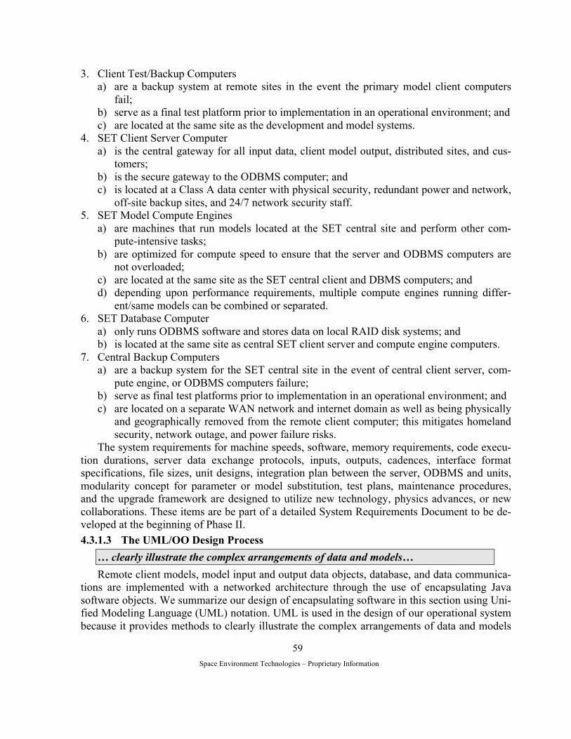
Space Environment Technologies – Proprietary Information
59
3. Client Test/Backup Computers a) are a backup system at remote sites in the event the primary model client computers
fail; b) serve as a final test platform prior to implementation in an operational environment; and c) are located at the same site as the development and model systems.
4. SET Client Server Computer a) is the central gateway for all input data, client model output, distributed sites, and cus-
tomers; b) is the secure gateway to the ODBMS computer; and c) is located at a Class A data center with physical security, redundant power and network,
off-site backup sites, and 24/7 network security staff. 5. SET Model Compute Engines
a) are machines that run models located at the SET central site and perform other com-pute-intensive tasks;
b) are optimized for compute speed to ensure that the server and ODBMS computers are not overloaded;
c) are located at the same site as the SET central client and DBMS computers; and d) depending upon performance requirements, multiple compute engines running differ-
ent/same models can be combined or separated. 6. SET Database Computer
a) only runs ODBMS software and stores data on local RAID disk systems; and b) is located at the same site as central SET client server and compute engine computers.
7. Central Backup Computers a) are a backup system for the SET central site in the event of central client server, com-
pute engine, or ODBMS computers failure; b) serve as final test platforms prior to implementation in an operational environment; and c) are located on a separate WAN network and internet domain as well as being physically
and geographically removed from the remote client computer; this mitigates homeland security, network outage, and power failure risks.
The system requirements for machine speeds, software, memory requirements, code execu-tion durations, server data exchange protocols, inputs, outputs, cadences, interface format specifications, file sizes, unit designs, integration plan between the server, ODBMS and units, modularity concept for parameter or model substitution, test plans, maintenance procedures, and the upgrade framework are designed to utilize new technology, physics advances, or new collaborations. These items are be part of a detailed System Requirements Document to be de-veloped at the beginning of Phase II. 4.3.1.3 The UML/OO Design Process
… clearly illustrate the complex arrangements of data and models… Remote client models, model input and output data objects, database, and data communica-
tions are implemented with a networked architecture through the use of encapsulating Java software objects. We summarize our design of encapsulating software in this section using Uni-fied Modeling Language (UML) notation. UML is used in the design of our operational system because it provides methods to clearly illustrate the complex arrangements of data and models

Space Environment Technologies – Proprietary Information
60
in a robust system. The UML diagrams and their related object-oriented concepts assume that the reader is fa-
miliar with the UML Object-Oriented (OO) design language. Even though UML has a well-defined taxonomy so that OO software (Java, C++) can be directly written using the figure elements of UML diagrams, the diagrams are also meant to be readable by those unfamiliar with UML terminology. For objects and methods, we use obvious names in our diagrams such as “F10inputObj,” “DateTimeClass,” and “getData.”
A complete UML design precedes our actual software programming and requires four types of diagrams specifying the operational software requirements: (1) use-case diagrams which are a thumb-nail, top-level view of all the project actors (people and subsystems) and their activi-ties; (2) physical design diagrams (also called deployment diagrams) showing the relationships between computers and their communication lines; (3) class and object diagrams (also called logical diagrams) which significantly expand on key components in the use-case diagrams and which largely define all the software objects attributes and methods; and (4) activity diagrams which show how operational scenarios are addressed. During the iterative diagramming process we have completed, loosely-coupled small abstract objects have become increasingly detailed with attributes, methods, and other OO elements for Phase II.
The detailed design of all OO elements will be completed during the first year of Phase II. However, as examples, key Use Cases as applied to input/output data, abbreviated Class defini-tions that expand on Use Cases, and activity diagrams that address specific operational scenar-ios are described below. The UML conventions for naming the components in our diagrams are based on Sinan [1998] and Booch [1994].
The input/output data objects present a large software design challenge in this project be-cause the collection of models have differing run cadences and complex, interdependent link-ages. Critical communication risks have been identified related to data stream outages or delays due to model failures, data concurrency and latency, computer and network failures, and soft-ware development and maintenance failures. We employ design patterns that are tailored to the data object requirements of a four-tier architecture to mitigate the risks. 4.3.2 Key Software Components
From the concept of operations, functional system design, physical architecture design, and UML/OO discussion, a number of “actors,” i.e., component systems that interact with other systems, have been identified. These are the server and database computers, compute engines or client host computers, as well as models and data which are all active within the component systems. For example, a client computer will communicate with the central server to access the database for getting input data and for delivering model results. Identifying these actors and their activities in a use case diagram allows us to identify objects that must be logically encap-sulated. This lays the basis for creating software that glues together a data communication sys-tem. We next discuss these key components and their relationship to data and model object properties and system redundancy. 4.3.2.1 Data and Model Object Properties
A first data or model object property is encapsulation since input and output data objects and model objects are encapsulated as single objects. A data object, for example, can contain a scalar, vector, or tensor that represents a past, present, or future time domain. The metadata
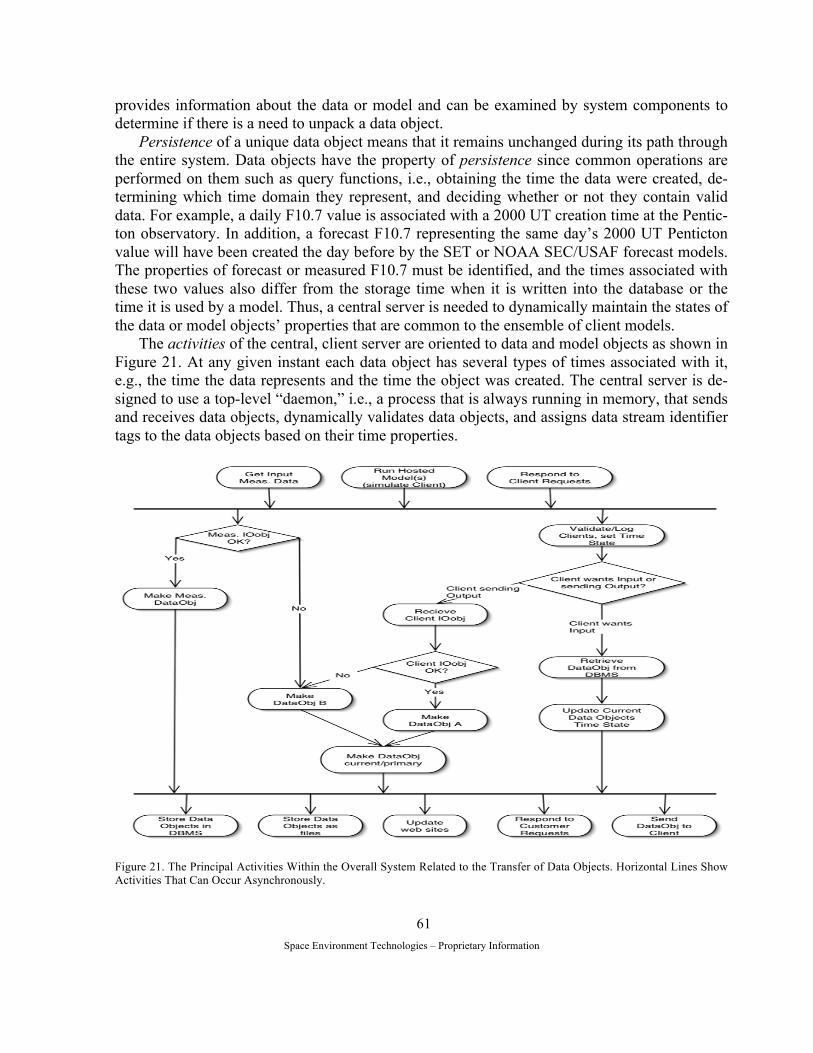
Space Environment Technologies – Proprietary Information
61
provides information about the data or model and can be examined by system components to determine if there is a need to unpack a data object.
Persistence of a unique data object means that it remains unchanged during its path through the entire system. Data objects have the property of persistence since common operations are performed on them such as query functions, i.e., obtaining the time the data were created, de-termining which time domain they represent, and deciding whether or not they contain valid data. For example, a daily F10.7 value is associated with a 2000 UT creation time at the Pentic-ton observatory. In addition, a forecast F10.7 representing the same day’s 2000 UT Penticton value will have been created the day before by the SET or NOAA SEC/USAF forecast models. The properties of forecast or measured F10.7 must be identified, and the times associated with these two values also differ from the storage time when it is written into the database or the time it is used by a model. Thus, a central server is needed to dynamically maintain the states of the data or model objects’ properties that are common to the ensemble of client models.
The activities of the central, client server are oriented to data and model objects as shown in Figure 21. At any given instant each data object has several types of times associated with it, e.g., the time the data represents and the time the object was created. The central server is de-signed to use a top-level “daemon,” i.e., a process that is always running in memory, that sends and receives data objects, dynamically validates data objects, and assigns data stream identifier tags to the data objects based on their time properties.
Figure 21. The Principal Activities Within the Overall System Related to the Transfer of Data Objects. Horizontal Lines Show Activities That Can Occur Asynchronously.
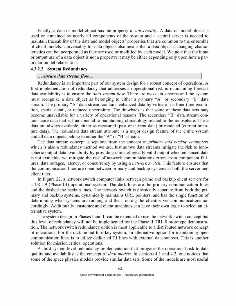
Space Environment Technologies – Proprietary Information
62
Finally, a data or model object has the property of universality. A data or model object is used or contained by nearly all components of the system and a central server is needed to maintain traceability of the data and model objects’ properties that are common to the ensemble of client models. Universality for data objects also means that a data object’s changing charac-teristics can be incorporated as they are used or modified by each model. We note that the input or output use of a data object is not a property; it may be either depending only upon how a par-ticular model relates to it. 4.3.2.2 System Redundancy
… ensure data stream flow… Redundancy is an important part of our system design for a robust concept of operations. A
first implementation of redundancy that addresses an operational risk in maintaining forecast data availability is to ensure the data stream flow. There are two data streams and the system must recognize a data object as belonging to either a primary “A” or secondary “B” data stream. The primary “A” data stream contains enhanced data by virtue of its finer time resolu-tion, spatial detail, or reduced uncertainty. The drawback is that some of these data sets may become unavailable for a variety of operational reasons. The secondary “B” data stream con-tains core data that is fundamental to maintaining climatology related to the ionosphere. These data are always available, either as measured (past or current data) or modeled (current or fu-ture data). The redundant data stream attribute is a major design feature of the entire system and all data objects belong to either the “A” or “B” stream.
The data stream concept is separate from the concept of primary and backup computers which is also a redundancy method we use. Just as two data streams mitigate the risk to iono-spheric output data availability by providing climatologically valid output when enhanced data is not available, we mitigate the risk of network communications errors from component fail-ures, data outages, latency, or concurrency by using a network switch. This feature ensures that the communication lines are open between primary and backup systems at both the server and client tiers.
In Figure 22, a network switch computer links between prime and backup client servers for a TRL 9 (Phase III) operational system. The dark lines are the primary communication lines and the dashed the backup lines. The network switch is physically separate from both the pri-mary and backup systems, dynamically maintains URL pointers, and has the single function of determining what systems are running and then routing the client/server communications ac-cordingly. Additionally, customer and client machines can have their own logic to select an al-ternative system.
The system design in Phases I and II can be extended to use the network switch concept but this level of redundancy will not be implemented for the Phase II TRL 8 prototype demonstra-tion. The network switch redundancy option is most applicable to a distributed network concept of operations. For the rack-mount turn-key system, an alternative option for maintaining open communication lines is to utilize dedicated T1 lines with external data sources. This is another solution for mission critical operations.
A third system-level redundancy implementation that mitigates the operational risk to data quality and availability is the concept of dual models. In sections 4.1 and 4.2, one notices that some of the space physics models provide similar data sets. Some of the models are most useful
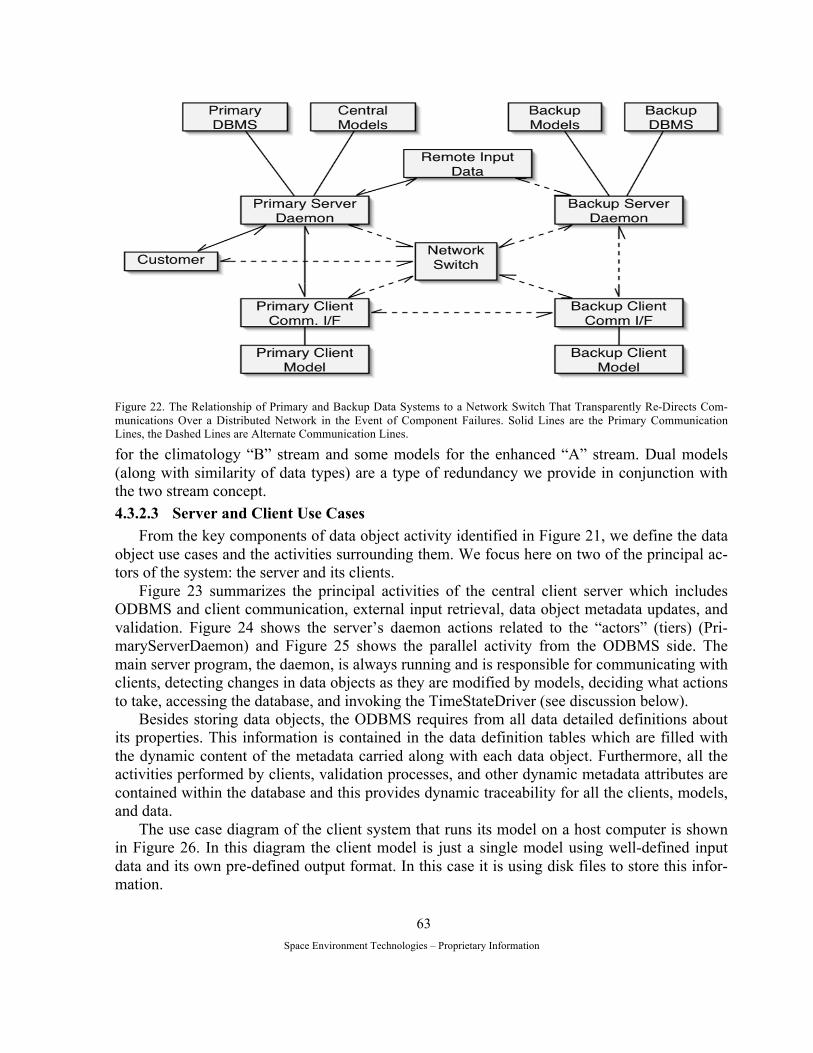
Space Environment Technologies – Proprietary Information
63
Figure 22. The Relationship of Primary and Backup Data Systems to a Network Switch That Transparently Re-Directs Com-munications Over a Distributed Network in the Event of Component Failures. Solid Lines are the Primary Communication Lines, the Dashed Lines are Alternate Communication Lines.
for the climatology “B” stream and some models for the enhanced “A” stream. Dual models (along with similarity of data types) are a type of redundancy we provide in conjunction with the two stream concept. 4.3.2.3 Server and Client Use Cases
From the key components of data object activity identified in Figure 21, we define the data object use cases and the activities surrounding them. We focus here on two of the principal ac-tors of the system: the server and its clients.
Figure 23 summarizes the principal activities of the central client server which includes ODBMS and client communication, external input retrieval, data object metadata updates, and validation. Figure 24 shows the server’s daemon actions related to the “actors” (tiers) (Pri-maryServerDaemon) and Figure 25 shows the parallel activity from the ODBMS side. The main server program, the daemon, is always running and is responsible for communicating with clients, detecting changes in data objects as they are modified by models, deciding what actions to take, accessing the database, and invoking the TimeStateDriver (see discussion below).
Besides storing data objects, the ODBMS requires from all data detailed definitions about its properties. This information is contained in the data definition tables which are filled with the dynamic content of the metadata carried along with each data object. Furthermore, all the activities performed by clients, validation processes, and other dynamic metadata attributes are contained within the database and this provides dynamic traceability for all the clients, models, and data.
The use case diagram of the client system that runs its model on a host computer is shown in Figure 26. In this diagram the client model is just a single model using well-defined input data and its own pre-defined output format. In this case it is using disk files to store this infor-mation.
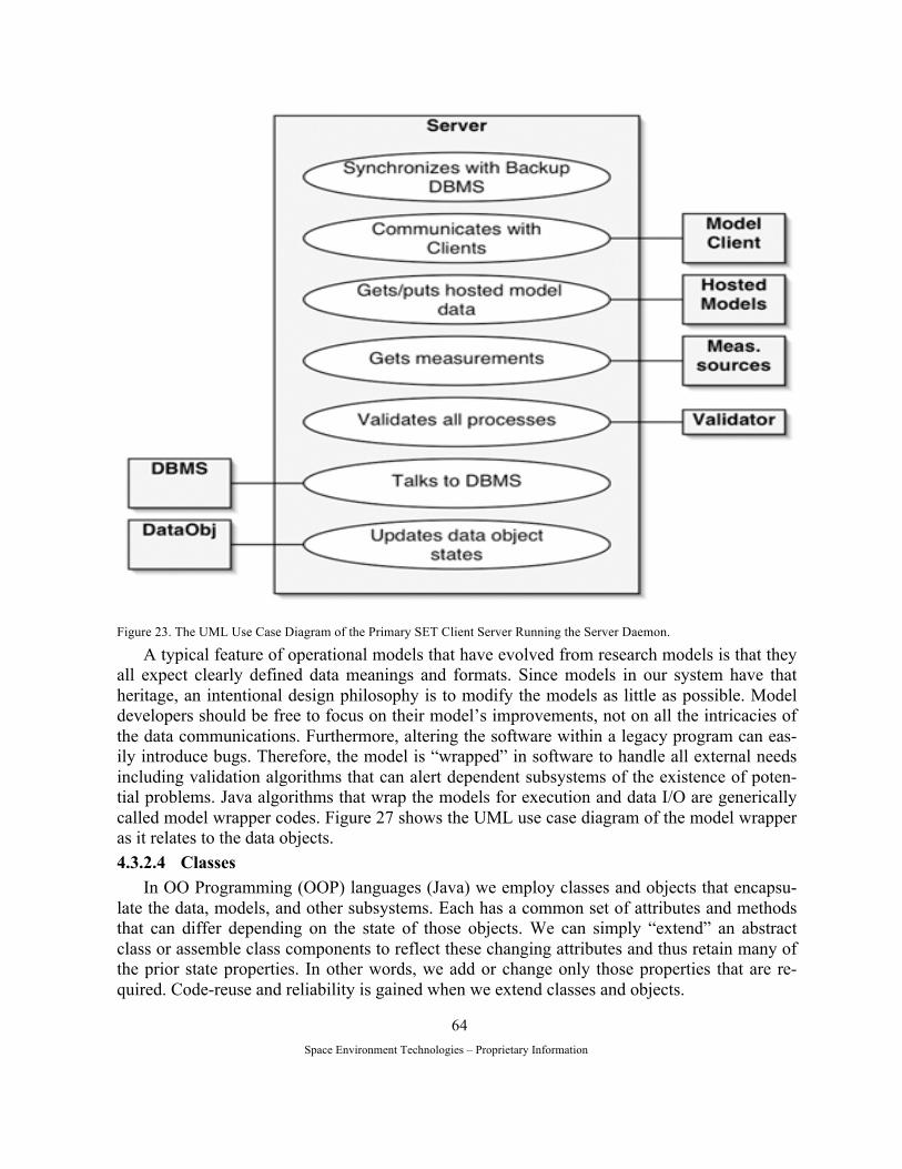
Space Environment Technologies – Proprietary Information
64
Figure 23. The UML Use Case Diagram of the Primary SET Client Server Running the Server Daemon.
A typical feature of operational models that have evolved from research models is that they all expect clearly defined data meanings and formats. Since models in our system have that heritage, an intentional design philosophy is to modify the models as little as possible. Model developers should be free to focus on their model’s improvements, not on all the intricacies of the data communications. Furthermore, altering the software within a legacy program can eas-ily introduce bugs. Therefore, the model is “wrapped” in software to handle all external needs including validation algorithms that can alert dependent subsystems of the existence of poten-tial problems. Java algorithms that wrap the models for execution and data I/O are generically called model wrapper codes. Figure 27 shows the UML use case diagram of the model wrapper as it relates to the data objects. 4.3.2.4 Classes
In OO Programming (OOP) languages (Java) we employ classes and objects that encapsu-late the data, models, and other subsystems. Each has a common set of attributes and methods that can differ depending on the state of those objects. We can simply “extend” an abstract class or assemble class components to reflect these changing attributes and thus retain many of the prior state properties. In other words, we add or change only those properties that are re-quired. Code-reuse and reliability is gained when we extend classes and objects.
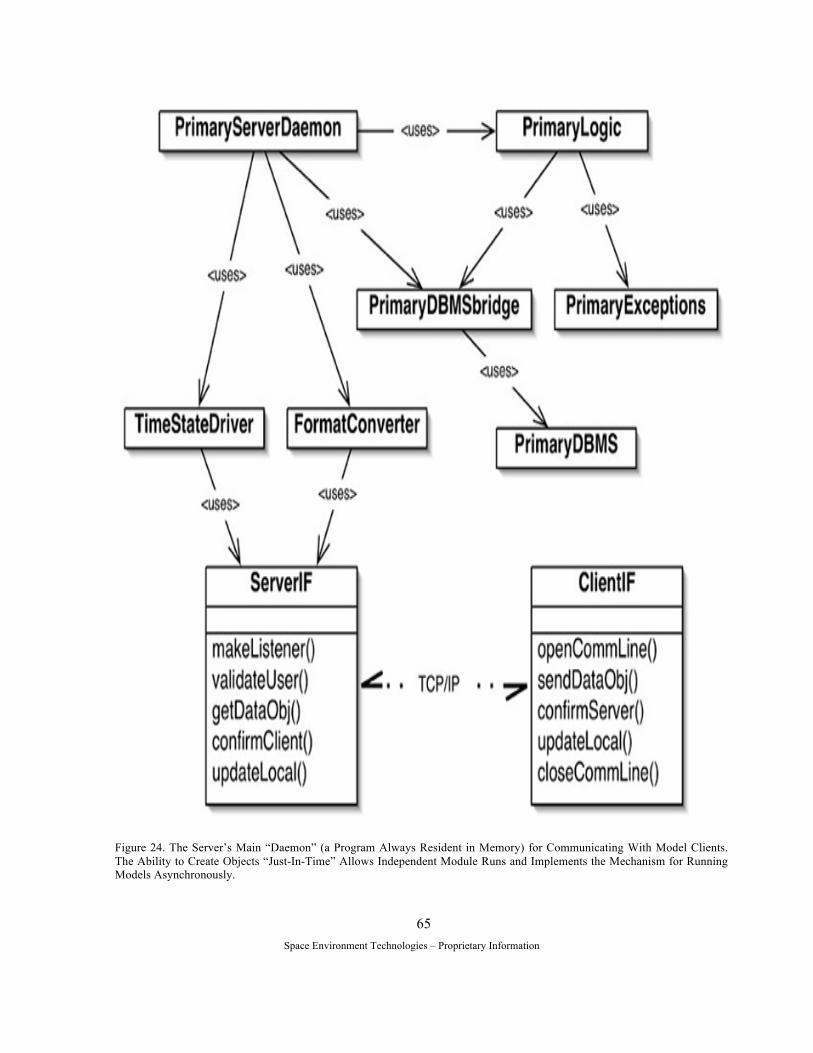
Space Environment Technologies – Proprietary Information
65
Figure 24. The Server’s Main “Daemon” (a Program Always Resident in Memory) for Communicating With Model Clients. The Ability to Create Objects “Just-In-Time” Allows Independent Module Runs and Implements the Mechanism for Running Models Asynchronously.

Space Environment Technologies – Proprietary Information
66
Figure 25. An Expanded View of the Use Cases Associated With the Central DBMS.
Figure 26. The UML Use Case Diagram of the Remote Client Computer Running a Model.
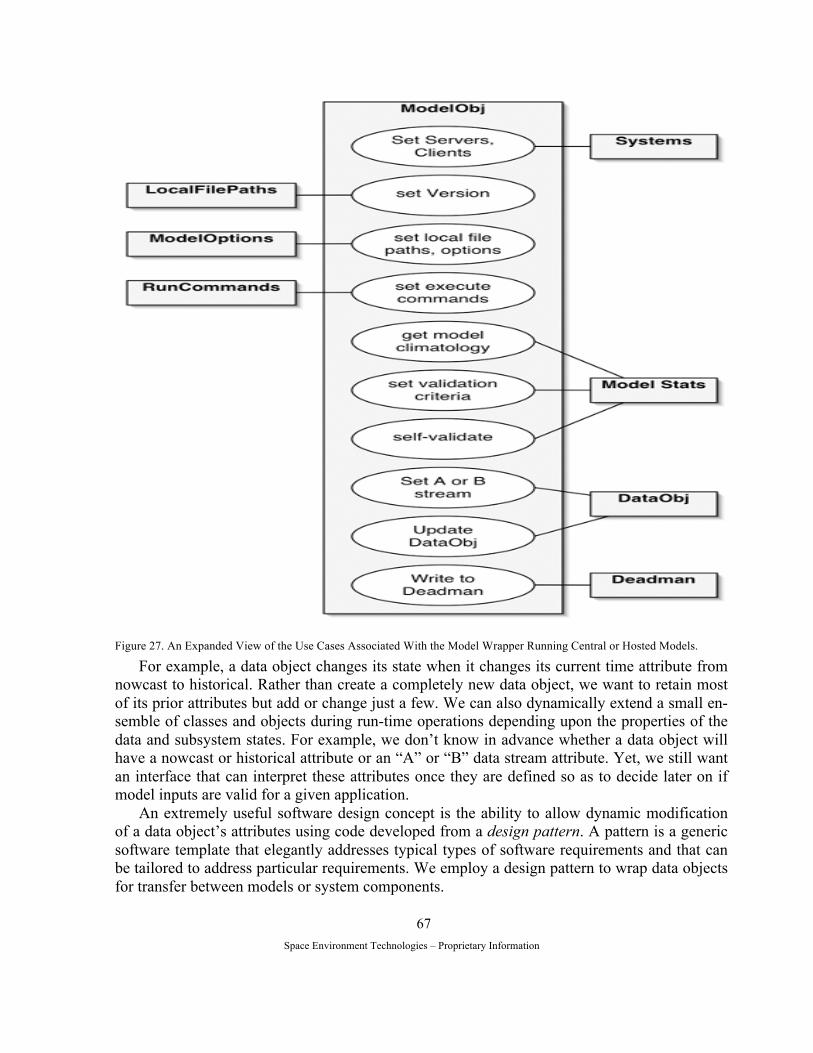
Space Environment Technologies – Proprietary Information
67
Figure 27. An Expanded View of the Use Cases Associated With the Model Wrapper Running Central or Hosted Models.
For example, a data object changes its state when it changes its current time attribute from nowcast to historical. Rather than create a completely new data object, we want to retain most of its prior attributes but add or change just a few. We can also dynamically extend a small en-semble of classes and objects during run-time operations depending upon the properties of the data and subsystem states. For example, we don’t know in advance whether a data object will have a nowcast or historical attribute or an “A” or “B” data stream attribute. Yet, we still want an interface that can interpret these attributes once they are defined so as to decide later on if model inputs are valid for a given application.
An extremely useful software design concept is the ability to allow dynamic modification of a data object’s attributes using code developed from a design pattern. A pattern is a generic software template that elegantly addresses typical types of software requirements and that can be tailored to address particular requirements. We employ a design pattern to wrap data objects for transfer between models or system components.

Space Environment Technologies – Proprietary Information
68
The Operational Ionospheric Forecast System has many data objects, models, system com-ponents, and even data streams that exist asynchronously or simultaneously. Because of this, time definition is a core attribute and redundancy is a core feature of this system. An abstract design pattern that can manage both the time attribute and redundancy features is an abstract factory design pattern. This is a set of classes that, depending on the current attributes of ob-jects, returns one of several families of subclasses to calling classes. For example, the S2KOP model system uses F10.7 as both an input and an output. In running the model, one set of input objects (historical and nowcast F10.7) will be used that have been “instantiated” (created) and another set of output objects (forecast F10.7) will be instantiated. These run-time classes of F10.7 data objects (“A” stream historical, nowcast, and forecast) are temporarily built from an abstract pattern (template) as soon as they are needed, they exist for some period of time, then disappear when they are no longer needed.
The Builder Design Pattern, which is derived from the Abstract Factory Design Pattern, is an ideal application for the family of data objects we are using in this project. We have selected the Builder Design Pattern as the template for data objects because it cleanly separates the data from model selection or run parameters. We have modified the generic Builder Design and Factory Design patterns to create templates that uniquely implement our own system’s flexible and robust qualities.
In Figure 28, we show these modified pattern concepts in a UML class diagram. A three-by-three matrix is shown that combines the time attribute with the redundancy feature. In this figure, time progresses along the vertical axis from the past (bottom) to the future (top) while the data streams that provide redundancy in data availability are separated along the horizontal axis. The “A” (left side) and “B” (right side) data streams are examples of the Builder Design pattern and each has slightly different qualities to describe enhanced or core characteristics, re-spectively. Both data streams derive from the higher level abstract factory pattern which is shown in the middle column. This matrix template, combining both time and redundancy, is the top level UML framework for all communication software in our operational system linking models with data objects.
In Figure 28, the terms “Forecast” vs. “Predicted,” “Nowcast” vs. “Current,” and “Histori-cal” vs. “Previous” are used to distinguish the different builder patterns based on past, present, and future time states. They are all extensions of the same foundation class but represent dis-tinctly different subclass families for the Enhanced (“A”) and Core (“B”) data objects. It is noted in OOP terminology that the word “extends” means an inheritance property (“is-a” type of relationship). For example, a Forecast class is a State Future class and it extends (employs) the methods of the parent level State Future class. The word “uses” is a composition property, i.e., a class can be a composite of other classes (“has-a” type of relationship). For example, a Predicted class has a Current class which has a Previous class.
… model developers do not have to redefine their data input, output parameters The design pattern concepts in Figure 28 are the fundamental component of data objects
and other classes throughout our system design. Figure 29, the TimeStateFactory collection of classes, shows the class diagram that implements the higher level Factory design pattern. A consequence of the TimeStateFactory pattern is that each client model object will have control of exactly how the model specifies it’s data IO and run parameters. This provides an enormous

Space Environment Technologies – Proprietary Information
69
Figure 28. The Top Level Factory and Builder Design Patterns That Provide a Template for Incorporating Lower Level Data Properties in Lower Level Classes. A Tip for Those Accustomed to Reading Flow-Charts: UML Diagrams Read from the “Bot-tom-Up” (Opposite to Direction of Arrows).
Figure 29. The Timestatefactory Builder Pattern That Employs the Factory Pattern in Figure 28.

Space Environment Technologies – Proprietary Information
70
time-saver for each team member’s model developers if they do not have to redefine their data input and output parameters. From a systems point-of-view it also provides a common platform (“suitcase”) for communication between system components. An additional consequence of this TimeStateFactory pattern is that each data stream is independent of the other and embed-ded data objects are independent of each other. This makes the program very modular and al-lows for easy addition of new or updated data sets and models.
The TimeStateDriver builder pattern class will be launched by the server every time a new data object is detected. This will create a family of classes based on whether the data refers to the past, present, or future. It does this by binding the TimeStateFactory class to a particular IOobject and this, in turn, extends the DataObj class (see below). The DataObj is the “data suit-case” sent between the server, ODBMS, and clients. Once the TimeStateFactory class instanti-ates a PastState, PresentState, or FutureState class it, in effect, creates a unique object. For ex-ample, the PresentState class would create a NowcastState object for stream “A” by extending the abstract StatePresent class. All of the methods that are specified in the TimeStateFactory such as get_DateTime() are available in the newly-formed NowcastState object.
Since the state of the family of classes (FutureState, PresentState, and PastState) refers to the attributes and values of an instantiated data object at a specific time (either Forecast or Pre-dicted, for example, depending on whether it is an A or B data stream object). In operations, the state of specific data sets and related classes will always be updating with new values added or changed as each measurement changes and each model operates asynchronously. There will always be a single current data object which is an instantaneous snapshot of all the data attrib-utes. 4.3.2.5 Data Objects
What do data objects actually look like? Like most other classes and their objects, the DataObj (super) class is composed of a number of other sub-classes. In the Operational Iono-spheric Forecast System, the DataObj class includes the scalar, vector, tensor data values for a single data type (termed “vector” here), the version of the last model that modified it, what formats it can use, and self-validating information. Figure 30 shows many of the objects that are contained within a DataObj class. In Figure 30, the integers within the lines indicate how many instances the parent class expects of each object. The use of “0,1” indicates the range of values of either “0” or “1.” For example, a DataObj must contain information on its parent (1) but does not necessarily need a serializer (0,1). There is no more than one instance of a child object with the exception of IOrecords. A vector is created in the IOvector and there can be any number of IOrecords in the vector. On the right-hand side of Figure 30 there are numerous classes shown that are used to validate key objects; this design allows any client or server to examine a data object for validity prior to use.
The detail of the IOobj subclass is shown in Figure 31. The IOrecord is contained within the IOobj class which has access to all the methods contained within the IOrecord. When an attribute is stored at the IOrecord level, all classes, including the PrimaryServerDaemon class in Figure 24, can make decisions about how to operate on or use the record. 4.3.3 Validation and Verification 4.3.3.1 Forecast Skills and Quality Monitoring
A key element in improving forecast accuracy is to continuously monitor forecast quality.

Space Environment Technologies – Proprietary Information
71
Forecast quality is measured by skill scores and several definitions of forecast skill exist in the meteorological community. We describe one technique below. Our system is designed to sys-tematically compute the forecast skill and therefore, provide a quality monitoring capability.
One important quality monitoring method is the ensemble forecast. As described in section 3.5, different forecast results based on different analyses provide an indication of forecast un-certainty. Similarly, perturbation of the ionospheric driving forces can also lead to different forecasts. In the case of initializing the ionospheric model using analyses, the difference in the forecast will usually diminish. However, this does not indicate an increase in forecast certainty but, instead, a lack of data. As a corollary, perturbation of driving forces from the non-GAIM models can lead to increased forecast differences and our design enables the creation of a fore-cast ensemble that can provide an estimate of forecast uncertainty. In our validation period dur-ing Phase II, the differences between E10.7 and F10.7 used in models can help provide an un-certainty, as an example.
Figure 30. Every Data Object (Dataobj) is a “Data Suitcase” Containing the Data Values, Metadata, and Methods for Other Systems and Programs to Retrieve the Contents. The Shaded Classes Are The Minimum Dataobj Sub-Classes Necessary for Model Inputs/Outputs, Resulting in a “Light-Weight” Dataobj Object Containing Mostly Data and a Few Essential Metadata Attributes.

Space Environment Technologies – Proprietary Information
72
Figure 31. One of the Family of Objects Contained Within the IOobj Class is the IOrecord. It Has All the Data Values, Their Individual Metadata Tags, and Methods That are to Validate Each Record. These are the Classes in Which the Actual In-put/Output Data Between Models and from External Sources are Contained and is the Principal Object Contained Within a “Data Suitcase.”
An important part of our Phase II work is to define an appropriate forecast skill. One of the candidates for forecast skill is the Normalized Cross Correlation coefficient defined by:
( )( )
( ) ( )∑ ∑
∑
= =
=
−⋅−
−⋅−=
N
k
N
k
aak
ffk
N
k
aak
ffk
nnnn
nnnn
1 1
22
1φ (3),
where fkn and fn are the forecast value at the k-th grid point and mean values over all forecast
point. Similarly, akn and an are the analysis values. One problem with the above skill is that if
fkn represents the ion density there is a great variability in ionospheric ion density. The above
skill is dominated by the large ion densities. Alternatively, we can replace fkn by f
kr where
ck
ck
fkf
k nnnr −
= (4).
The quantity ckn is the climatological value for the ion density.
Space Environment Technologies – Proprietary Information
73
Another problem with skills defined above is that if there are no data available between forecast and analysis times, the forecast skill would be perfect. However, this is a common problem with most of forecast skills. The final definition of forecast skill requires consensus in the ionospheric research community. Our project provides a valuable test-bed for forecast skill metrics and this is an area of potential work in our collaboration with NOAA SEC.
It is important to indicate the difference between computation of forecast skill and direct validation of a forecast. In direct validation, we compare a forecast ionospheric quantity to the measured quantity. This provides an absolute measurement on the accuracy of the forecast. However, the difference between the forecast values and the actual measurement includes two types of errors. The first is the analysis error. In this case, the data assimilation provides an analysis of the ionospheric condition based on the modeled physics and the ensemble of all available data. This analysis represents the best physically self-consistent interpretation of the data. The second error is forecast error. The forecast skill attempts to characterize the forecast error. The systematic evaluation of the forecast skill provides us with valuable information about how to improve the accuracy of the forecast. 4.3.3.2 GAIM Accuracy Validation
To forecast the ionospheric state accurately, one must also “nowcast” accurately. The accu-racy of GAIM assimilations and the resulting electron density specifications have already been validated in three ways: (1) by a series of simulation experiments in which a known iono-spheric density field is used to generate synthetic input data for simulated assimilation runs; (2) by a series of validation case studies using actual input datasets and multiple kinds of validation data; and (3) by continuous validation of daily operational Kalman filter runs beginning in March of 2003.
Simulation. For the simulation experiments, the electron density field and the appropriate values of the drivers (e.g., equatorial E×B vertical drift, neutral winds, and production terms) are known and can be compared to the values estimated by GAIM after input of the synthetic data. For example, we have demonstrated that using only ground GPS TEC links one can gain sufficient information about the shape and location of the equatorial anomaly arcs to estimate E×B vertical drift values as a function of local time and a grid of neutral wind values in geo-magnetic coordinates (see Pi et al., 2003 and recent 4DVAR talks available on the GAIM web site).
Validation Cases. For case studies using real input datasets, the true ionospheric state is not known so the accuracy of the electron density specification is evaluated by comparisons to independent ionospheric observations and/or alternative density retrieval techniques. Major validation case studies have been performed for five types or combinations of input data as-similated by GAIM: (1) absolute TEC data from ground GPS receivers (global network); (2) relative TEC data from GPS occultations (flight receivers on IOX, CHAMP, and SAC-C); (3) radiance data from nighttime FUV limb scans (LORAAS instrument on ARGOS); (4) ground GPS TEC combined with GPS occultations; and (5) ground GPS combined with UV limb scans. The combined data runs are particularly relevant to future operational scenarios in which the ground GPS network provides good overall global TEC coverage and dense coverage in some regions, but limited vertical resolution, while GPS occultations from the planned six-satellite COSMIC constellation and UV scans from the SSUSI and SSULI instruments on

Space Environment Technologies – Proprietary Information
74
DMSP provide detailed regional data with excellent vertical resolution. The accuracy validation studies have included comparisons to: vertical TEC measurements
from the TOPEX and JASON dual-frequency ocean altimeters (1330 km altitude), slant TEC measurements from independent GPS sites, FoF2 and HmF2 values or bottom-side profiles from ionosondes, density profiles from incoherent scatter radars, density profiles obtained from Abel inversions of GPS occultations (alternative retrieval technique), and two-dimensional density retrievals (in the plane of the ARGOS satellite orbit) computed by the NRL UV group using Chapman layers. Examples of each of these kinds of validation are documented in the papers and presentations available on the USC/JPL GAIM web site.
Continuous Daily Validation. In order to start accumulating long-term accuracy statistics for GAIM density specification, daily runs of the global Kalman filter began in March of 2003. Each day GAIM assimilates more than 200,000 ground GPS TEC observations from 98+ sites to specify the ionospheric density state. The intent is to continuously validate GAIM accuracy as input data types are added (UV radiances or GPS occultations) along with improved drivers from the other operational models. The validation process will be completely automated and performed every day as part of several assimilation runs. Forecast and nowcast accuracy cannot be established by one-time case studies but must be continuously monitored.
Several validation comparisons are already being automated so that accuracy statistics ac-cumulate for every hour and day. They include comparisons to vertical TEC from TOPEX or JASON, to slant TEC from independent GPS sites that probe a variety of latitude and longitude sectors, and to foF2 and HmF2 observations from global ionosonde sites. New JASON data are available every 3-4 hours and the data from independent GPS sites are collected either hourly or daily so accuracy can be monitored every few hours and statistics accumulated daily. The public ionosonde data are delayed but the accuracy of yesterday’s ionospheric specification can be evaluated with a 1-day delay along with the skill score for the 24-hour ionospheric forecast.
As an example of the on-going validation, consider Figure 32 which shows a comparison of GAIM results to TOPEX vertical TEC observations on March 12, 2003. Figure 32 (top) shows the 98 GPS sites used as input for the assimilation and a daytime TOPEX track passing near Hawaii. To perform the comparison, the GAIM density grid is integrated vertically to predict the vertical TEC at the exact location of each TOPEX observation. Figure 32 (bottom) com-pares the measured TOPEX TEC (+ symbol) to the predicted TEC values from: (1) the GAIM assimilation (x symbol); (2) the GAIM “climate” (open square, no data input to the model); (3) the IRI95 model (solid square); and (4) the two-dimensional TEC maps from the JPL GIM model (x symbol, using the same 98 GPS sites). Note that the GAIM assimilation result follows the two equatorial anomaly peaks quite well as well as the trough between them and the more gradual mid-latitude gradients. The RMS differences for this track are 4.9 TEC units (1016 el/m2) for the GAIM assimilation versus 11.3 TECU for the GAIM climate and 12.2 TECU for IRI95.
By accumulating the differences (GAIM minus vertical TEC measurements) for all of the TOPEX or JASON tracks each day, one can compute a daily RMS error for the low-, mid-, and high-latitude regions. Note that TOPEX and JASON only probe a fixed local time on any given day. Figure 33 shows the daily RMS errors for more than half of a year, March 11 to October 17, 2003. In the top plot the model RMS errors versus day of year for observations with latitude below 30 degrees are given while in the bottom plot the RMS error for the mid- and high-

Space Environment Technologies – Proprietary Information
75
Figure 32. (Top) TOPEX Satellite Track on March 12, 2003; (Bottom) Comparison of TOPEX Vertical TEC Observations With Four Models, TEC Versus Geographic Latitude.

Space Environment Technologies – Proprietary Information
76
5
10
15
20
50 100 150 200 250
TOPEX Comparison for GAIM, GIM, and IRI95:Low Latitudes
GIMGAIM ClimateIRI95GAIM Assim
RMS V
TEC D
ifferen
ces (M
odel -
TOPE
X)
2003 DOY(Mar 11 - Oct 17)
5
10
15
20
50 100 150 200 250
TOPEX Comparison for GAIM, GIM, and IRI95:Mid & High Latitudes
GIMGAIM ClimateIRI95GAIM Assim
RMS V
TEC D
ifferen
ces (M
odel -
TOPE
X)
2003 DOY(Mar 11 - Oct 17)
Figure 33. Daily RMS Differences (Model Minus TOPEX) for Four Models: GAIM Assimilation (Open Square), GAIM Cli-mate (Open Triangle), IRI95 (Solid Triangle), and JPL GIM (Solid Circle). (Top) Low-Latitudes, (Bottom) Mid- and High-Latitudes Combined.
Space Environment Technologies – Proprietary Information
77
latitude observations combined is shown. Note that the GAIM assimilation accuracy is quanti-tatively better than the GAIM climate or IRI95 with often 3-7 TECU in the low-latitudes and 3-5 TECU in the mid- and high-latitudes. The variation in the error during the period is a combi-nation of several effects including seasonal dependence of the ionosphere (spring and fall iono-sphere levels versus summer), quiet versus disturbed days, and the change in the local time probed by TOPEX. 4.3.3.3 Operational Software Validation
We have designed our system to track and maintain information about the current state of the analysis and forecast errors of the physical representation of the ionosphere as described above. We use imbedded validation methods and flags associated with each record and encap-sulating objects to do this. In addition, we perform a second type of validation monitoring, i.e., that of the “state of health” of the current operating system. To track the physics representation and operating system indicators, we use a validation daemon. The Validator daemon (a con-tinually running process) is based on a SET-developed design pattern for validating multiple asynchronous processes. Imbedded validation methods and flags provide information such as geophysical limits on input data and current forecast skill so that a process can decide if the data object is valid. The Validator daemon runs a set of processes that monitor the system-level communications and interim data object validation results. In Figure 34 the Validator daemon monitors all the input data and model data quality, can detect fatal program errors, and sets metadata flags in each object at their creation which enables subsequent programs to make de-cisions based on the validation flags. Decisions about which data stream to use or whether or not to notify an operator of a significant problem are also made based on the Validator daemon actions.
The entire system’s operation can be summarized in a single code number, character, or expression. The Validator class requires every process to create, update, and close a “Deadman” file
during its execution. This file contains diagnostic information and flags describing the run status of every process. As a sidebar, the word “Deadman” was chosen based on the old “Deadman switch” used by train engineers; if the engineer ever let go of the switch, the train would automatically stop. The Deadman classes are conceptual relatives, i.e., if anything goes wrong, a Deadman file exists that contains information to locate the point of failure. The top-level Validator class then uses a “ToeTagger” class to analyze all the existing Deadman files and the ToeTagger information contains the summary status of the entire system’s operation. In addition, a unique feature of our system is that the Validator class produces one overall run status flag based on the ensemble of Deadman files and run status flags in the DataObj. If the ToeTagger class and run status flags indicate there are no problems in any of the Deadman files or DataObj, we are guaranteed that all models have been validated. The entire system’s current state can be summarized in a single code number, character, or expression. 4.3.3.4 Validation Intent
The design for this system incorporates the validation activities described above to ensure that the data objects meet their specified requirements or fall within acceptable, pre-defined limits during operations. Each model developer provides the limits of validity for input and

Space Environment Technologies – Proprietary Information
78
Figure 34. The Use Cases of a Validator Daemon Which Validates Data Objects and Obtains the Run Status of All Other Proc-esses Including Model Runs; It Provides the Information To the ODBMS To Allow Traceability.
output data and these are tracked in the appropriate classes. Usually, the values are defined with geophysical limits (minimum and maximum values). Additionally, some data types will be judged in relation to whether or not they are statistically near the expected values (n-sigma, Δt, mean). Other data types will meet a requirement to be statistically equivalent to similar data types (n%, r). The validation class contains, where appropriate, the selection criteria for “bet-
Space Environment Technologies – Proprietary Information
79
ter” if two similar data types are compared (comparison scale). The Phase II requirements documents will detail the format and values of these validation activities and parameters. 4.3.3.5 Verification Intent
Following validation, the system design enables us to determine if the data output objects meet the intent of the requirements. In a daily post-analysis of the GAIM output data (1-2 day lag), for example, we will provide ongoing skill scores comparing forecasts with actual iono-spheric parameters. Prior to operations, much of the testing and validation work in Phase II will provide a baseline for verifying the climatological forecast output of the operational iono-spheric forecast system. Verification will primarily be performed with independent data and model comparisons. 4.3.3.6 Testing Intent
A component and system end-to-end test plan will be developed in months 6-12 of Phase II (Table 1 Key Milestones, Figure 35c). We will also identify metrics for evaluating system per-formance and for validation and verification of output product accuracy, precision, and error. Comparative independent data will be reviewed and collected to aid with the prototype’s evaluation while use-case scenarios will be evaluated to test for operational anomalies. A strat-egy for modular validation, verification, and self-testing of upgraded elements, once the system is operational beyond the prototype stage, is being considered as a Phase III activity. 4.3.3.7 Team Practices
Our team uses best engineering practices consistent with Capability Maturity Model (CMM) Level 2 processes to meet operational requirements. As the lead organization, SET’s engineering practices have proven successful in four research model-to-operations transitions since the mid 1990’s: (1,2) the Magnetospheric Specification Model (MSM) and the SO-LAR2000 models implemented at NOAA SEC in Boulder; (3) the proprietary SET commercial server; and (4) the USAF HASDM project. 4.3.4 Upgrades, Maintenance Strategy
Our team will consider an upgrade and system maintenance design strategy as an activity in the last six months of Phase II. Our implementation strategy for Phase II uses modular valida-tion, verification, and testing of upgraded system elements once the system is declared opera-tional. When models are modular units that can be upgraded or replaced, then the upgrade framework can take advantage of new technology, advanced physics, and extended collabora-tions. Modularity allows upgrades to occur easily on a component by component basis. This guideline lays the foundation for long-term system and product evolution. 4.3.5 Risk Management
During any portion of project life cycle, risks emerge that can significantly affect the sys-tem or software design. We use Technology Readiness Level (TRL) definitions as the highest level risk management tool for ensuring a successful life cycle. It describes the life cycle of a project going from initial concept to successful operational implementation. Many projects can have a very long TRL lifetime (years) from low- to high-TRL levels. In the worst case, a risk area with a low-TRL level has the potential of making it impossible to complete the project with the financial resources available. We begin our life cycle risk management by starting with models that are at mid-TRL levels and data streams that are at high-TRL levels. We ex-
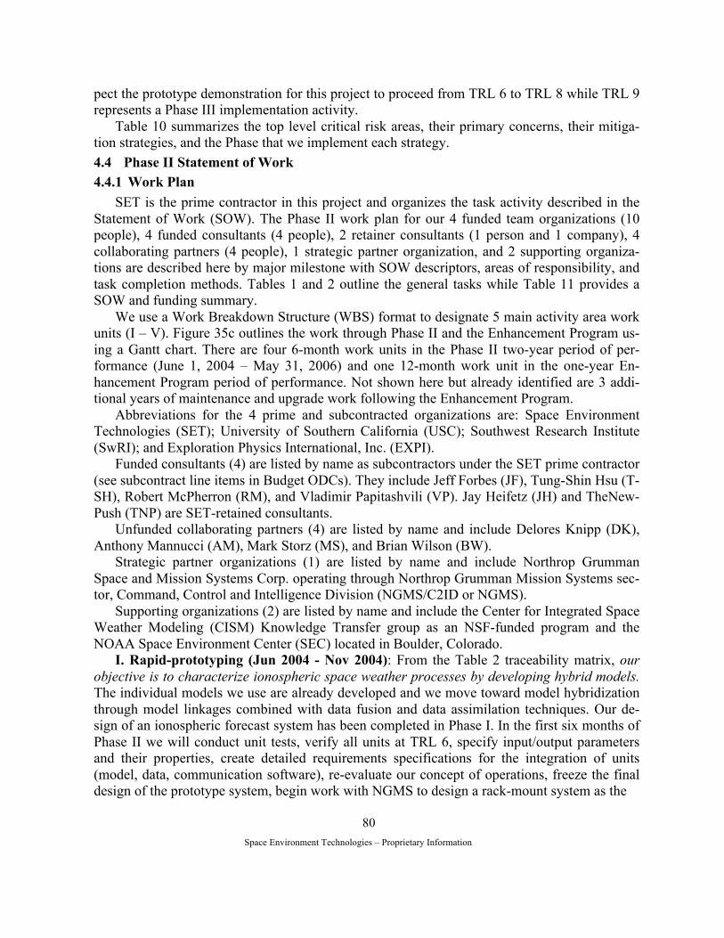
Space Environment Technologies – Proprietary Information
80
pect the prototype demonstration for this project to proceed from TRL 6 to TRL 8 while TRL 9 represents a Phase III implementation activity.
Table 10 summarizes the top level critical risk areas, their primary concerns, their mitiga-tion strategies, and the Phase that we implement each strategy. 4.4 Phase II Statement of Work 4.4.1 Work Plan
SET is the prime contractor in this project and organizes the task activity described in the Statement of Work (SOW). The Phase II work plan for our 4 funded team organizations (10 people), 4 funded consultants (4 people), 2 retainer consultants (1 person and 1 company), 4 collaborating partners (4 people), 1 strategic partner organization, and 2 supporting organiza-tions are described here by major milestone with SOW descriptors, areas of responsibility, and task completion methods. Tables 1 and 2 outline the general tasks while Table 11 provides a SOW and funding summary.
We use a Work Breakdown Structure (WBS) format to designate 5 main activity area work units (I – V). Figure 35c outlines the work through Phase II and the Enhancement Program us-ing a Gantt chart. There are four 6-month work units in the Phase II two-year period of per-formance (June 1, 2004 – May 31, 2006) and one 12-month work unit in the one-year En-hancement Program period of performance. Not shown here but already identified are 3 addi-tional years of maintenance and upgrade work following the Enhancement Program.
Abbreviations for the 4 prime and subcontracted organizations are: Space Environment Technologies (SET); University of Southern California (USC); Southwest Research Institute (SwRI); and Exploration Physics International, Inc. (EXPI).
Funded consultants (4) are listed by name as subcontractors under the SET prime contractor (see subcontract line items in Budget ODCs). They include Jeff Forbes (JF), Tung-Shin Hsu (T-SH), Robert McPherron (RM), and Vladimir Papitashvili (VP). Jay Heifetz (JH) and TheNew-Push (TNP) are SET-retained consultants.
Unfunded collaborating partners (4) are listed by name and include Delores Knipp (DK), Anthony Mannucci (AM), Mark Storz (MS), and Brian Wilson (BW).
Strategic partner organizations (1) are listed by name and include Northrop Grumman Space and Mission Systems Corp. operating through Northrop Grumman Mission Systems sec-tor, Command, Control and Intelligence Division (NGMS/C2ID or NGMS).
Supporting organizations (2) are listed by name and include the Center for Integrated Space Weather Modeling (CISM) Knowledge Transfer group as an NSF-funded program and the NOAA Space Environment Center (SEC) located in Boulder, Colorado.
I. Rapid-prototyping (Jun 2004 - Nov 2004): From the Table 2 traceability matrix, our objective is to characterize ionospheric space weather processes by developing hybrid models. The individual models we use are already developed and we move toward model hybridization through model linkages combined with data fusion and data assimilation techniques. Our de-sign of an ionospheric forecast system has been completed in Phase I. In the first six months of Phase II we will conduct unit tests, verify all units at TRL 6, specify input/output parameters and their properties, create detailed requirements specifications for the integration of units (model, data, communication software), re-evaluate our concept of operations, freeze the final design of the prototype system, begin work with NGMS to design a rack-mount system as the

Space Environment Technologies – Proprietary Information
81
Table 10. Critical Risks and Mitigation Critical risk areas and concerns Mitigation strategy Mitigation Addressed
Scientific validity and quality 1) geophysically valid parameters 2) accurate and precise parameters 3) incorporation of new physics
1) validation tests conducted in Phase II; highly time variable
parameters (particle fluxes, Dst, Ap, B, w, for example) may be less reliable and we will improve some of them in the En-hancement Program
2) validation tests can be built into the software to permit auto-mated alternate actions in the event of exceptions to normal operations
3) model modularity enables new physics insertion
1) Phases II-III 2) Phases II-III 3) Phases I-III
System forecast operations 1) single points of failure 2) component failures, data dropouts, la-
tency, concurrency 3) complexity of operations and network
1a) design two streams “A” and “B” for dual redundancy;
models linkage is through an independent data base with dy-namic input and output of data resources; models run asyn-chronously at their native cadence, execution time, and envi-ronment
1b) develop a network switch to guarantee operational robust-ness
2) design two streams “A” and “B” for dual redundancy; use model climatology in the event of dropouts, latency; embody graceful degradation; stream “B” is always available, either measured or modeled
3) track, log, and report on the operational state of the entire system with validator daemon; maintain knowledge of the overall operational state and network communications; sum-marize system state with code value
1a) Phase I 1b) Phase III 2) Phase I 3) Phase I
Software reliability 1) data object JIT transfer 2) data stream outages or delays from
model failures, data concurrency and latency, computer and network com-munication failures
3) software development failures 4) maintenance failures 5) operational upgrade failures
1) four-tier data communication system architecture for transfer
of input/output data objects enables continuous availability 2) dual data stream, dual models or data sets, central and backup
computers
3) unit and end-to-end system testing and validation using proven software
4) validator daemon process captures and reports exceptions 5) testing for operational upgrades on backup machines
1) Phase I 2) Phase II 3) Phase II 4) Phase I 5) Phase II
Hardware robustness 1) central client server, compute engine,
or DBMS computer failure 2) external environment to operational
system has network outages and power failures
1) central and backup computers 2) central and backup computers physically separated; use
dedicated communication lines
1) Phase I 2) Phase III
Project management 1) maintain geographically separated
team with diverse members from dif-ferent institutional cultures
1) hold team teleconferences on regular basis, conduct site visits
and face-to-face meetings as necessary; use prime contractor and subcontractor funding relationship
1) Phases I, II
Financial 1) funding “valley of death” moving from
low to high TRL levels 2) satisfy diverse institutional funding
and intellectual property requirements
1) start with data streams at TRL 8 or 9 and models at TRL 6 or
higher 2) negotiate IP and license agreements early in project
1) Phase I 2) Phases I, II
Schedule 1) incorporate diverse data sets, models,
and hardware/software systems in a coordinated project to achieve proto-type (TRL 8) level by the project com-pletion date
1) start at mid or high TRL levels for models and data; use
COTS software for all major software components and well-proven hardware systems that require minimal system ad-ministration
1) Phase I
Commercialization 1) identify strategic partners to achieve
contracts with identifiable customers for specific product deliveries
1) start strategic partner discussions in Phase I for effective
relationships in Phase II
1) Phase I

Space Environment Technologies – Proprietary Information
82
derivative of a distributed network, and conduct a Critical Design Review. SET coordinates with team members: 1. (USC, SwRI, EXPI, JF, T-SH, RM, VP, DK, AM, MS, BW) collection of TRL 6 unit
tests on development machines; 2. (USC, SwRI, EXPI, JF, T-SH, RM, VP, DK, AM, MS, BW) collection of input/output
parameters and their properties; 3. (USC, SwRI, EXPI, JF, T-SH, RM, VP, DK, AM, MS, BW, SEC, TNP) detailed re-
quirements specifications for unit integration (model, data, communication software); 4. (USC, SwRI, EXPI, JF, T-SH, RM, VP, DK, AM, MS, BW, SEC, NGMS) re-
evaluation of concept of operations; 5. (NGMS, TNP) design a rack-mount system as the derivative of a distributed network;
and 6. (USC, SwRI, EXPI, JF, T-SH, RM, VP, DK, AM, MS, BW, SEC, NGMS, CISM, TNP,
JH) Critical Design Review. USC coordinates: GAIM model TRL 6 unit test; collection of input/output parameters and
their properties; and detailed requirements specifications for the integration of units (model, data, communication software).
SwRI coordinates: particle precipitation model TRL 6 unit test; collection of input/output parameters and their properties; and detailed requirements specifications for the integra-tion of units (model, data, communication software).
EXPI coordinates: HAF model TRL 6 unit test; collection of input/output parameters and their properties; and detailed requirements specifications for the integration of units (model, data, communication software).
II. System design and development (Dec 2004 - May 2005): From Table 2, our objective is to develop ionospheric space weather applications based on research models that we transi-tion into operations. As we build an ionospheric forecast system in the second six months, we will make all major hardware and software purchases, test the server and database, finish de-velopment of data communication software, integrate and assemble the units as a prototype sys-tem platform, begin linked unit testing, test data communication software, refine software, de-velop a system test plan, continue system design document and user manual preparation, con-tinue work with NGMS to design a rack-mount system, and conduct a Pre-Test Review.
SET coordinates with team members: 1. (TNP) major hardware and software purchases; 2. (USC, SwRI, EXPI, TNP) test the server, database, client machines; 3. (USC, SwRI, EXPI, JF, T-SH, RM, VP, DK, AM, MS, BW, TNP) finish development
of data communication software; 4. (USC, SwRI, EXPI, JF, T-SH, RM, VP, DK, AM, MS, BW, TNP) integrate and assem-
ble the units as a prototype system platform; 5. (USC, SwRI, EXPI, JF, T-SH, RM, VP, DK, AM, MS, BW, TNP) test unit links; 6. (USC, SwRI, EXPI, JF, T-SH, RM, VP, DK, AM, MS, BW, TNP) test data communi-
cation software; 7. (USC, SwRI, EXPI, JF, T-SH, RM, VP, DK, AM, MS, BW, TNP) refine all software; 8. (USC, SwRI, EXPI, JF, T-SH, RM, VP, DK, AM, MS, BW, TNP) develop a system test
plan;

Space Environment Technologies – Proprietary Information
83
Figure 35a. Gantt Chart View of the Project Phase I, Part 1.

Space Environment Technologies – Proprietary Information
84
Figure 35b. Gantt Chart View of the Project Phase I, Part 2.

Space Environment Technologies – Proprietary Information
85
Figure 35c. Gantt Chart View of the Project Phase II and Enhancement Program.

Space Environment Technologies – Proprietary Information
86
Table 11. Team SOW Summary Teams, related models, other tasks Phase 2 funding
Space Environment Technologies (SET): SOLAR2000, 1DTD, NRLMSIS00, J70MOD, HWM93, joule heating, OM2000, Ap, DICM; central server; ODBMS database; IT and parameter transfer software; ConOps development; test management; documentation management; project management
50% funded organization
University of Southern California (USC): GAIM, EUV94X, NRLMSIS00, HWM93, HM87, SF99, W95 34% funded organization
AM, BW (Jet Propulsion Laboratory {JPL}): GAIM, EUV94X, NRLMSIS00, HWM93, HM87, SF99, W95 {,GPS TEC}
no-fee collaborators
Southwest Research Institute (SwRI): particle precipitation 6% funded organization
Exploration Physics International, Inc. (EXPI): HAF 3% funded organization
VP (Geomagnetic Services {GS}): DICM 3% funded consultant
T-SH, RM (University of California, LA {UCLA}): OM2000, Ap 3% funded consultant
JF (University of Colorado {CU}): neutral winds {HWM93} 1% funded consultant
JH (HC): business strategy development SET-retained consultant
TNP: server hosting facility SET-retained consultant
MS (Air Force Space Command XPY): J70MOD no-fee collaborator
DK (US Air Force Academy {USAFA}): Joule heating no-fee collaborator
NGMS: rack-mount system design strategic partner
NOAA SEC: use nowcast products supporting organization
CISM: use of archive data supporting organization
9. (USC, SwRI, EXPI, JF, T-SH, RM, VP, DK, AM, MS, BW, TNP, NGMS, SEC, CISM) continue preparation of a system design document and user manual;
10. (NGMS, TNP) continue design of rack-mount system; and 11. (USC, SwRI, EXPI, JF, T-SH, RM, VP, DK, AM, MS, BW, SEC, NGMS, CISM, TNP,
JH) Pre-Test Review. USC coordinates: GAIM model integrate and assemble with prototype system platform; test
links; test data communication; refine software; preparation of user manual (GAIM sec-tion).
SwRI coordinates: particle precipitation model integrate and assemble with prototype sys-tem platform; test links; test data communication; refine software; preparation of user manual (particle precipitation section).
EXPI coordinates: HAF model integrate and assemble with prototype system platform; test links; test data communication; refine software; preparation of user manual (HAF sec-tion).
III. Testing (Jun 2005 - Nov 2005): From Table 2, our objective is to test an operational ionospheric forecast system. We will verify that the system is at TRL 7, conduct complete in-put/output parameter tests, conduct an integrated system test, conduct performance tests and quantify errors/uncertainty, develop verification, error, and performance metrics, refine docu-mentation, continue work with NGMS to design a rack-mount system, and conduct a Customer Requirements Review.
SET coordinates with team members: 1. (USC, SwRI, EXPI, JF, T-SH, RM, VP, DK, AM, MS, BW, TNP) verify system at TRL
7; 2. (USC, SwRI, EXPI, JF, T-SH, RM, VP, DK, AM, MS, BW, TNP) conduct complete

Space Environment Technologies – Proprietary Information
87
input/output parameter tests; 3. (USC, SwRI, EXPI, JF, T-SH, RM, VP, DK, AM, MS, BW, TNP) conduct integrated
system test; 4. (USC, SwRI, EXPI, JF, T-SH, RM, VP, DK, AM, MS, BW, TNP) conduct performance
tests and quantify errors/uncertainty; 5. (USC, SwRI, EXPI, JF, T-SH, RM, VP, DK, AM, MS, BW, NGMS, SEC, CISM, TNP)
develop verification, error, and performance metrics; 6. (USC, SwRI, EXPI, JF, T-SH, RM, VP, DK, AM, MS, BW, NGMS, SEC, CISM, TNP)
refine documentation; 7. (NGMS, TNP) continue to design a rack-mount system; and 8. (USC, SwRI, EXPI, JF, T-SH, RM, VP, DK, AM, MS, BW, SEC, NGMS, CISM, TNP,
JH) Customer Requirements Review. USC coordinates: GAIM model verify at TRL 7; participate in complete input parameter
tests; participate in integrated system test; participate in performance tests and quantify errors/uncertainty; participate in verification, error, and performance metrics develop-ment; refine GAIM documentation.
SwRI coordinates: particle precipitation model verify at TRL 7; participate in complete in-put parameter tests; participate in integrated system test; participate in performance tests and quantify errors/uncertainty; participate in verification, error, and performance metrics development; refine particle precipitation documentation.
EXPI coordinates: HAF model verify at TRL 7; participate in complete input parameter tests; participate in integrated system test; participate in performance tests and quantify errors/uncertainty; participate in verification, error, and performance metrics develop-ment; refine HAF documentation.
IV. Validation and verification (Dec 2005- May 2006): From Table 2, our objective in developing ionospheric space weather applications is to successfully demonstrate our proto-type and educate potential customers. We will fully exercise the system to validate its function-ing per design requirements and to verify its output according to our stated intent using estab-lished metrics, develop an upgrade and maintenance plan, prepare final documents and user manual, conduct a burn-in and prototype demonstration, verify the prototype operational iono-spheric forecast system is at TRL 8, continue work with NGMS to design a rack-mount system, and conduct a customer delivery review.
SET coordinates with team members: 1. (USC, SwRI, EXPI, JF, T-SH, RM, VP, DK, AM, MS, BW, NGMS, SEC, TNP) fully
exercise the system and validate its functioning per design requirements; 2. (USC, SwRI, EXPI, JF, T-SH, RM, VP, DK, AM, MS, BW, NGMS, SEC, CISM, TNP)
verify system output according to stated intent using established metrics; 3. (USC, SwRI, EXPI, JF, T-SH, RM, VP, DK, AM, MS, BW, NGMS, SEC, TNP) de-
velop an upgrade and maintenance plan; 4. (USC, SwRI, EXPI, JF, T-SH, RM, VP, DK, AM, MS, BW, NGMS, SEC, CISM, TNP)
prepare final documents and user manual; 5. (USC, SwRI, EXPI, JF, T-SH, RM, VP, DK, AM, MS, BW, NGMS, SEC, CISM, TNP,
JH) conduct burn-in and prototype demonstration; 6. (USC, SwRI, EXPI, JF, T-SH, RM, VP, DK, AM, MS, BW, NGMS, SEC, CISM, TNP,

Space Environment Technologies – Proprietary Information
88
JH) verify the prototype operational ionospheric forecast system is at TRL 8; 7. (NGMS, TNP) continue to design a rack-mount system; and 8. (USC, SwRI, EXPI, JF, T-SH, RM, VP, DK, AM, MS, BW, NGMS, SEC, CISM, TNP,
JH) conduct a customer delivery review. USC coordinates: GAIM model fully exercised to validate its functioning per design re-
quirements; verify GAIM output according to stated intent using established metrics; de-velop upgrade and maintenance plan; prepare final documents and GAIM training guide.
SwRI coordinates: particle precipitation model fully exercised to validate its functioning per design requirements; verify particle precipitation output according to stated intent us-ing established metrics; develop upgrade and maintenance plan; prepare final documents and particle precipitation training guide.
EXPI coordinates: HAF model fully exercised to validate its functioning per design re-quirements; verify HAF output according to stated intent using established metrics; de-velop upgrade and maintenance plan; prepare final documents and HAF training guide.
V. Enhancement Program (Jun 2006- May 2007): From Table 2, our objective is to serve ionospheric space weather customers by providing space weather operational systems.
To improve scientific representation of the ionosphere, we will update the SwRI particle precipitation model by including NOAA-15, NOAA-16 data and by including an algorithm to distinguish between Dst parameter storm main phase and recovery periods for use by the SwRI model. We will invite the Utah State University GAIM team to actively work with us to pro-vide system level redundancy in ionospheric specification. We will work with the CISM com-munity to provide archival data in return for knowledge transfer from their project to ours.
Moving towards operations, and along with our NGMS partner, we will build, test, deliver, and maintain a clustered turn-key, rack-mount system that could be located at AFWA. From our distributed network system, we would provide nowcasts of ionospheric parameters and space environment information to our NOAA SEC supporting partner. As part of this activity, we will conduct a customer requirement re-review, assist an independent risk review, conduct a customer modification review, and develop an upgrade plan.
SET coordinates with team members: 1. (USC, SwRI, AM, BW, SEC, CISM) update SwRI particle precipitation model by in-
cluding NOAA-15, NOAA-16 data; 2. (USC, SwRI, AM, BW, T-SH, RM, SEC, CISM) update SwRI particle precipitation
model by including an algorithm to distinguish between Dst parameter storm main phase and recovery periods;
3. (USC, AM, BW, SEC, CISM, NGMS) invite the Utah State University GAIM team to actively work with team to provide system level redundancy in ionospheric specifica-tion;
4. (CISM) work with CISM community to provide archival data in return for knowledge transfer from their project to ours;
5. (NGMS) build rack-mount system; 6. (NGMS) test rack-mount system; 7. (NGMS) deliver rack-mount system; 8. (USC, SwRI, EXPI, JF, T-SH, RM, VP, DK, AM, MS, BW, NGMS) maintain rack-
mount system;

Space Environment Technologies – Proprietary Information
89
9. (NGMS, SEC, CISM) provide nowcasts of ionospheric parameters and space environ-ment information to NOAA SEC;
10. (USC, SwRI, EXPI, JF, T-SH, RM, VP, DK, AM, MS, BW, NGMS, SEC, CISM, TNP, JH) customer requirement re-review;
11. (USC, SwRI, EXPI, JF, T-SH, RM, VP, DK, AM, MS, BW, NGMS, SEC, CISM, TNP, JH) assist independent risk review;
12. (USC, SwRI, EXPI, JF, T-SH, RM, VP, DK, AM, MS, BW, NGMS, SEC, CISM, TNP, JH) conduct customer modification review;
13. (USC, SwRI, EXPI, JF, T-SH, RM, VP, DK, AM, MS, BW, NGMS, SEC, CISM, TNP, JH) develop upgrade plan
USC coordinates: GAIM model test with updated SwRI particle precipitation model that in-cludes NOAA-15, NOAA-16 data; test with updated SwRI particle precipitation model that includes an algorithm to distinguish between Dst parameter storm main phase and re-covery periods; participate with USU GAIM team to provide system level redundancy in ionospheric specification; review CISM community knowledge transfer items; consult on rack-mount system maintenance; consult on provision of nowcasts of ionospheric pa-rameters and space environment information to NOAA SEC; consult on upgrade plan.
SwRI coordinates: particle precipitation model test with updated NOAA-15, NOAA-16 data; test algorithm to distinguish between Dst parameter storm main phase and recovery periods; review CISM community knowledge transfer items; consult on rack-mount sys-tem maintenance; consult on provision of nowcasts of ionospheric parameters and space environment information to NOAA SEC; consult on upgrade plan.
EXPI coordinates: review CISM community knowledge transfer items; consult on rack-mount system maintenance; consult on provision of nowcasts of ionospheric parameters and space environment information to NOAA SEC; consult on upgrade plan.
4.4.2 Safety Our work plan uses purchased COTS software and hardware (computer) systems where no
hardware is to be developed. In terms of safety requirements, each institution maintains its own safety program as appropriate to its circumstances. There are no extra-ordinary safety issues associated with the software development and network connectivity that is the basis for our sys-tem. The facilities we use for hosting the prototype system are Class A commercial server facil-ity with its own security and safety procedures. There is no requirement for providing a Pre-liminary Hazard Analysis (PHA) Report and there are no potentially hazardous materials that could result in risk to personnel or property used in this project. 4.5 Phase II Deliverables
In Table 12 we show deliverables by milestone (WBS, task name), organization, deliver-able item, and delivery date. The final deliverable is a prototype demonstration of the opera-tional ionospheric forecast system and a final technical report. The final report will identify the purpose of the work, details of the project objectives, a description of the work accomplished, the findings or results, review of technical feasibility, and expected applications of our effort. Because this system is a distributed network and involves leveraged prototype computing and software resources from several organizations across the country, no hardware or software is delivered at the project end.
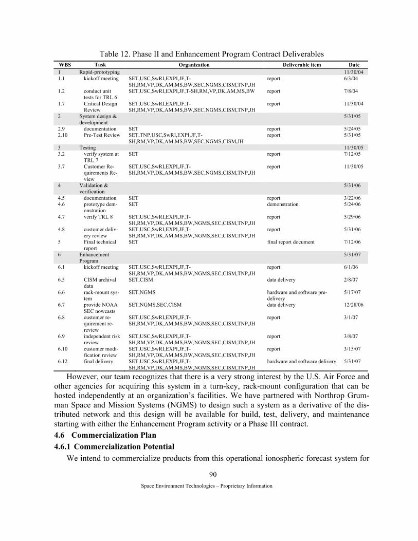
Space Environment Technologies – Proprietary Information
90
Table 12. Phase II and Enhancement Program Contract Deliverables WBS Task Organization Deliverable item Date 1 Rapid-prototyping 11/30/04 1.1 kickoff meeting SET,USC,SwRI,EXPI,JF,T-
SH,RM,VP,DK,AM,MS,BW,SEC,NGMS,CISM,TNP,JH report 6/3/04
1.2 conduct unit tests for TRL 6
SET,USC,SwRI,EXPI,JF,T-SH,RM,VP,DK,AM,MS,BW report 7/8/04
1.7 Critical Design Review
SET,USC,SwRI,EXPI,JF,T-SH,RM,VP,DK,AM,MS,BW,SEC,NGMS,CISM,TNP,JH
report 11/30/04
2 System design & development
5/31/05
2.9 documentation SET report 5/24/05 2.10 Pre-Test Review SET,TNP,USC,SwRI,EXPI,JF,T-
SH,RM,VP,DK,AM,MS,BW,SEC,NGMS,CISM,JH report 5/31/05
3 Testing 11/30/05 3.2 verify system at
TRL 7 SET report 7/12/05
3.7 Customer Re-quirements Re-view
SET,USC,SwRI,EXPI,JF,T-SH,RM,VP,DK,AM,MS,BW,SEC,NGMS,CISM,TNP,JH
report 11/30/05
4 Validation & verification
5/31/06
4.5 documentation SET report 3/22/06 4.6 prototype dem-
onstration SET demonstration 5/24/06
4.7 verify TRL 8 SET,USC,SwRI,EXPI,JF,T-SH,RM,VP,DK,AM,MS,BW,NGMS,SEC,CISM,TNP,JH
report 5/29/06
4.8 customer deliv-ery review
SET,USC,SwRI,EXPI,JF,T-SH,RM,VP,DK,AM,MS,BW,NGMS,SEC,CISM,TNP,JH
report 5/31/06
5 Final technical report
SET final report document 7/12/06
6 Enhancement Program
5/31/07
6.1 kickoff meeting SET,USC,SwRI,EXPI,JF,T-SH,RM,VP,DK,AM,MS,BW,NGMS,SEC,CISM,TNP,JH
report 6/1/06
6.5 CISM archival data
SET,CISM data delivery 2/8/07
6.6 rack-mount sys-tem
SET,NGMS hardware and software pre-delivery
5/17/07
6.7 provide NOAA SEC nowcasts
SET,NGMS,SEC,CISM data delivery 12/28/06
6.8 customer re-quirement re-review
SET,USC,SwRI,EXPI,JF,T-SH,RM,VP,DK,AM,MS,BW,NGMS,SEC,CISM,TNP,JH
report 3/1/07
6.9 independent risk review
SET,USC,SwRI,EXPI,JF,T-SH,RM,VP,DK,AM,MS,BW,NGMS,SEC,CISM,TNP,JH
report 3/8/07
6.10 customer modi-fication review
SET,USC,SwRI,EXPI,JF,T-SH,RM,VP,DK,AM,MS,BW,NGMS,SEC,CISM,TNP,JH
report 3/15/07
6.12 final delivery SET,USC,SwRI,EXPI,JF,T-SH,RM,VP,DK,AM,MS,BW,NGMS,SEC,CISM,TNP,JH
hardware and software delivery 5/31/07
However, our team recognizes that there is a very strong interest by the U.S. Air Force and other agencies for acquiring this system in a turn-key, rack-mount configuration that can be hosted independently at an organization’s facilities. We have partnered with Northrop Grum-man Space and Mission Systems (NGMS) to design such a system as a derivative of the dis-tributed network and this design will be available for build, test, delivery, and maintenance starting with either the Enhancement Program activity or a Phase III contract. 4.6 Commercialization Plan 4.6.1 Commercialization Potential
We intend to commercialize products from this operational ionospheric forecast system for
Space Environment Technologies – Proprietary Information
91
candidate industries including DoD agencies, GPS providers and users, aviation, electric-power distribution systems, satellite operators, telecommunications providers, and public science mu-seums. Our team provides two lines of evidence for commercial potential: the existence of SET’s (small business) commercialization strategy and Phase III follow-on commitments for an operational ionospheric forecast system. In describing our commercialization strategy, we pre-sent our market analysis, our market strategy, and partner strategy. The latter includes Phase III follow-on commitments by third parties for developing a commercial basis for operational ionospheric forecast system products. Our commercialization effort is strengthened because our strategic partner is closely aligned with a primary customer. We round out our commercializa-tion strategy discussion by briefly reviewing our competitors and our business model. 4.6.2 Market Analysis
We conduct our market analysis from the perspective of what is our market position, who are the potential customers, what are the market constraints, and what is the market size that will dictate the product development strategy. 4.6.2.1 Market Position
Our commercialization effort enjoys the position of being “first-mover” for the prototype implementation of an operational ionospheric forecast system. We consider this a strong advan-tage in a market that is newly forming with growth potential. 4.6.2.2 Potential Customers
Our immediate focus area is the DoD customer who uses radar, high-frequency radio com-munications, geolocation technologies, and GPS navigation systems. In a longer term view, there is a parallel customer base in the civilian sector. We have developed an initial list of or-ganizations and industries which we see as prime customers early in Phase III. They are the fol-lowing:
(a) Air Force Weather Agency (AFWA). AFWA is the U.S. Department of Defense (DoD) supplier to U.S. armed forces for their ionospheric needs. They are located at Of-fut AFB in Omaha, Nebraska. We expect AFWA to award a contract in FY 05-06 to implement an operational ionospheric forecast system based on the GAIM model and AFWA will likely use NGMS as its prime contractor, a position that it currently holds. We see AFWA as our first and primary, but not only, customer for a fully operational ionospheric forecast system.
(b) NOAA Space Environment Center (SEC). NOAA SEC in Boulder, Colorado is an agency that has clearly and publicly expressed interest, on several occasions, for build-ing a civilian counterpart to the potential AFWA operational ionospheric forecast sys-tem. While there are no funds identified for implementation of this capability at NOAA SEC, and they are in the midst of a major organizational transition into the NOAA Na-tional Weather Service (NWS), we believe SEC will remain interested in acquiring the capabilities of an operational ionospheric forecast system. SEC has provided this project with strong support and our team, during Phase II, will hold detailed discussions with SEC to provide some of our system’s capability to them. A candidate option is to pro-vide free to SEC for civilian use nowcast ionospheric and other space environment pa-rameters in exchange for a CRADA-type agreement allowing competition-free forecast-ing for a defined period of time. This arrangement has been used in the past to nurture a

Space Environment Technologies – Proprietary Information
92
U.S. space weather industry. (c) GPS Navigation Providers and Users. There are many, many companies in the agri-
cultural, oil/gas exploration and production, and transportation industries that currently use or are developing civilian GPS navigation capabilities. Example companies include Trimble, Omnistar (US and South America), UPS, FedEx, ocean container shippers, air cargo carriers, and personal navigation system owners whose access to GPS signals is denied or inaccurate due to ionospheric phenomena. For single-frequency GPS users (nearly all civilian and many DoD users), GPS-derived position accuracy is an issue. This is also true for differential GPS (DGPS) and real-time kinematic (RTK) applica-tions since the ionospheric term in satellite signal observation equations may not cancel; this creates solution ambiguities and an opportunity for improvement. The potential contract amount for systems-level or consumer derivative products (TEC) is very large and will grow larger in the future. It is probable that established companies providing GPS equipment or solutions can be strategic partners for accessing larger markets. With this in mind, SET has begun preliminary contacts in December 2003 with Trimble, a medium-sized company that is a leading innovator of GPS technology. In addition to providing advanced GPS components, Trimble augments GPS with other positioning technologies as well as wireless communications and software to create complete cus-tomer solutions. Trimble’s worldwide presence and unique capabilities position them for growth in emerging applications including surveying, automobile navigation, ma-chine guidance, asset tracking, wireless platforms, and telecommunications infrastruc-ture. SET understands that the products of the operational ionospheric forecast system can enhance Trimble’s business sector. SET will also establish contact with another GPS firm, Novetel, in the event Trimble is not interested in our products.
(d) Geolocation Users. A growing industry exists to precisely locate people and objects us-ing GPS technology. This market, a derivative of the GPS navigation market, will likely grow in the future; strategic partners would be companies already providing consumer products. Systems-level derivative products (TEC) are a likely growth area.
(e) Weather Information Providers. We are aware of an interest, among organizations such as The Weather Channel, to expand their weather service content by including some space weather phenomena. SET, in the fall of 2003, began preliminary contacts with The Weather Channel to explore mutual areas of interest.
(f) Aviation Carriers. Commercial and civil aviation carriers use polar routes that are sub-ject to periodic HF communications anomalies and outages. Companies that are active in this area include commercial airlines, private executive jets, charter services, bush pi-lots, and local or regional emergency response services. Two long-term partners of our team from previous proposals, RPSI (a small business) and ARINC (a medium size business), can aid in developing products and customers for improved HF capabilities based on operational ionospheric forecasts. The size of this market for systems-level de-rivative products (HF MUF, HmF2, f0F2) is not known but expected to remain rela-tively stable or grow modestly in the future. Terrorism has targeted commercial airlines and this has reduced that industry’s use of polar routes in the near-term. SET will reini-tiate contact with both RPSI and ARINC in 2004 to develop partnering strategies for use of this system’s products.
Space Environment Technologies – Proprietary Information
93
(g) Power Distribution Companies. Power distribution companies, especially those serv-ing customers in northern latitudes, face conditions where electrical energy delivery can be interrupted by ground-induced currents resulting from space weather effects on the Earth’s electric field. The companies most affected are located in Europe, Canada, the northern U.S., Scandinavia, and Russia. In 2004, we intend to strategically partner with Metatech (a small company) who has been a space weather collaborator in the past and is actively serving this industry. The market size for systems-level derivative products (electric field potentials) is expected to remain stable or grow slightly.
(h) Satellite Operators. Low Earth orbit satellite constellation operators are responsible for operational knowledge of the location and functioning of their satellite assets. For issues related to spacecraft communications, charging, attitude, and orbit determination related to satellite drag and maintenance of constellation formations using GPS, satellite opera-tors want to know ionospheric and thermospheric conditions. It is likely that the market will continue to grow at a slow rate in the future. There are several companies offering satellite operational software and they would be strategic partners for expanding a set of derivative products (thermospheric densities, TEC, solar constant, particle fluxes, HmF2, f0F2). These companies include Analytic Graphics (Satellite Toolkit software), Microcosm (Orbit Control Kit, Advanced High Precision Orbit Propagation, and Sat-Life software), and a.i. Solutions. SET has begun discussions with each of these three companies during the past two years on related topics and will expand those discussion in 2004 with topics related to this work. Orbcomm and DigitalGlobe are commercial satellite operators who are customers of these companies and would benefit from im-proved software products.
(i) Imagery Providers. There is a rapidly growing market for satellite and high altitude aerial hyperspectral imagery products. User industries include agriculture, defense, and urban planning, for example. Precision operational solar spectral information in the near UV, visible, and infrared wavelengths is a very promising candidate for calibration of hyperspectral imagery; detector calibration is necessary to extract subtle information content from images. Kodak is actively working on the satellite imaging technology, has shown clear interest in using the Sun as a calibration source, and SOLAR2000 v4.00, to be validated in part through this work, will provide this capability. Research efforts will take an additional 2 years if funding is found to achieve this capability. The market size is expected to grow substantially in this area and strategic partners include scientific (NCAR/HAO), instrument (Kodak), and satellite (DigitalGlobe).
(j) Telecommunications Providers. Wireless telecommunications may be affected by space weather events. There has been some hint of a correlation between wireless transmitter interference and solar radio bursts during the past few years, especially dur-ing high solar activity. However, the physics are not well-understood which makes solu-tions to wireless telecommunications outages non-existent at the present time with the exception of HF radio. Given the huge and growing size of the telecommunications market, this would be an attractive area for derivative products if the physics were bet-ter understood. There is a continuing, long-term international scientific effort to under-stand wireless telecommunication outages.
(k) Science Museums. World class and national museums, as well as the scientific and

Space Environment Technologies – Proprietary Information
94
public education communities, have expressed continued interest in acquiring iono-spheric data for educational and research resources. This market is likely to continue with modest growth in the future; strategic partner organizations include the Smith-sonian Museum or Hayden Planetarium to provide historical or near real-time exhibits of the global conditions. SET understands that it is in the best interest of this team to foster public education about space weather and will seek to rekindle contacts with both museum organizations that were first started in 2000.
4.6.2.3 Market Constraints The outputs of the operational ionospheric forecast system and some of its developmental
pieces are regulated under the U.S. State Department’s International Traffic in Arms Regula-tions (ITAR) export controls for sales to users outside of the U.S. This represents an impedi-ment to foreign sales from an additional cost of doing business or a prohibition of export. It may be possible to offer some derivative products for foreign commercial applications.
Market education is certainly an issue; many potential customers don’t yet understand the market or know that there is a need for ionospheric products. In some cases, ionospheric needs have yet to be demonstrated. We will continue to support efforts of scientific study and public education about space weather.
A near-term legal constraint exists where licensing and intellectual property agreements must be in place with all of the system’s contributors and software owners by the end of Phase II. 4.6.2.4 Market Size
As noted in section 4.6.2.2 (Potential Customers), there is an extremely large market for the products which we will offer. It is not possible at this point to estimate the size other than to say billions of dollars of assets can benefit from our information and revenue could easily be in the millions of dollars within a decade. 4.6.3 Market Strategy
A key criteria for product development is its revenue potential, i.e., how quickly can a product generate revenue? An initial method of generating rapid revenue with new products is based upon the approach of marketing “low-hanging fruit” early in Phase III. “Low-hanging fruit” are products that take little effort to develop and for which there are current customers, known potential customers, clearly identified needs for and benefits from such products, and secondary customers for whom it will be inexpensive to modify what has already been devel-oped for primary customers. 4.6.3.1 First Product
The primary product we will create after the end of Phase II is a derivative of the distrib-uted network operational ionospheric forecast system prototype. That derivative is a rack-mount/turn-key fully operational ionospheric forecast system for our first customer. We expect that first customer to be AFWA although we recognize that AFWA must still be convinced of our system’s utility for them. 4.6.3.2 Follow-on Products
Separately, using the distributed network TRL 8 prototype at the end of Phase II that will be transitioned into TRL 9 operations by SET and its partners, we will develop commercial prod-

Space Environment Technologies – Proprietary Information
95
ucts in many formats including educational, informational, alert, and warning status with spa-tial and time information. Specific products include: slant and vertical TEC; HmF2; f0F2; MUF; GPS uncertainty maps; electric field potentials; electron, ion, and neutral species’ densi-ties; thermospheric mass densities; thermospheric temperatures; thermospheric neutral winds; solar radiation pressure; integrated and spectral solar irradiances; solar wind shock arrival times; solar wind and Earth magnetosphere particle fluxes; auroral boundaries; surface charg-ing probabilities; proton events; and cosmic ray fluxes.
Our ionospheric products will contain refined information relative to raw input data; they are, in fact, intermediate data products that are only modestly useful by themselves. If coupled with other applications, the utility of these data become greatly magnified. The discussion in section 4.6.4.2 related to operational partnering provides more insight on how we intend to pur-sue product development and implementation. 4.6.3.3 Capitalization Strategy
We have studied a variety of capitalization (funding) options for advancing this project be-yond Phase II and into Phase III commercialization. We understand that crossing this funding “valley-of-death” is a serious risk for many projects. We have mitigated this risk in our project by starting with technology that is at the TRL 6 or higher level, aiming for a TRL 8 prototype demonstration at the end of 2+ years (Phases I and II), and identifying a methodology by which to generate revenue. That methodology is: identify a prime customer, develop a product spe-cifically suited to that customer, and organize our activity to meet that customer’s needs in the time frame defined by the customer. For our operational ionospheric forecast system, AFWA is the prime Phase III customer and a rack-mount/turn-key system is a likely product suited to that customer.
Given this direction, we have looked at funding options that will enhance the success of ob-taining this customer. We have considered angel investors, venture capital funds, and large as well as small corporate partners. In general, we have found that venture capital (VC) is a lim-ited or non-existent funding source in the aerospace industry for new technology development. Angel investors, as with VC funds, require an exit strategy that does not serve the development of our system, in our opinion. Exit strategies for angel investors and VCs rely heavily on Initial Public Offerings (IPOs) or mergers/acquisitions to recoup up to 10 times a return on investment in a performance period of 2-5 years. On the other hand, strategic corporate partners often find that investment in low- or mid-TRL technologies is a cost-effective method of fulfilling aligned or committed R&D goals in a risk avoidance climate.
Our project, at the beginning of Phase II, is a mid-TRL technology, is in a “first-mover” po-sition with respect to implementation of the technology, and represents a relatively modest in-vestment that is leveraged by government funding through the Phase II SBIR. These factors combine to make the operational ionospheric forecast system technology very attractive for large corporate partners. We have identified one large aerospace corporate partner that can be a strategic partner and this is NGMS. A Confidential Disclosure Agreement was signed by NGMS and SET. It demonstrates a commitment by a large aerospace company to explore commercialization issues related to this project. 4.6.3.4 High Level Development Process
Our team is continually refining its market analysis, market strategy, partner strategy, com-
Space Environment Technologies – Proprietary Information
96
petitor analysis, and business model. In Phase II we will initiate partnering agreements and cus-tomer contacts as well as tailor ionospheric forecast system output products to meet unique cus-tomer requirements. We will define these requirements in Phase II by conducting a customer prototype demonstration of the distributed network and, with NGMS strategic partner assis-tance, will develop a design of the rack-mount turn-key system. As a follow-up to the prototype demonstration, we will evaluate customer comments and assess the technical merits for product modification. For feasible modifications, a prioritization plan will be developed in conjunction with the writing of a statement of work for Phase III implementation followed by the drafting of a requirements document. The latter will use the TRL 8 documentation developed in Phase II as a foundation.
Customer contract negotiations will be initiated in late Phase II for identifiable products that customers are interested in. Negotiable items include contract labor and services, licensing agreement(s), customer-specific ionospheric forecast system installations or data product deliv-eries, customer training session(s), maintenance and upgrade schedules, and installation or product delivery sign-off dates. 4.6.4 Partner Strategy
We describe our partnering relationships for scientific improvement of our system, for op-erations, and for marketing. 4.6.4.1 Team Partners in Science
We have formalized science partnerships in this Phase II proposal based upon defined areas of expertise. Team partners include researchers from USC, JPL, SwRI, EXPI, UCLA, GS, CU, USAF SPC/XPY, and USAFA. These team members are active in space physics research espe-cially as related to improving operational ionospheric forecasting. Each of these members has ongoing research activity outside this project.
We have added the Center for Integrated Space Weather Modeling (CISM) Knowledge Transfer group as a supporting member of our team in Phase II. CISM is the national leading program, sponsored by the NSF, to develop physics-based models over the next decade that can quantify and reproduce the elements of the Sun-Earth connection as related to space weather. We will provide the CISM community with archival data from our system and will be a recipi-ent of their physics-based models that can improve space weather specification and forecasting over the next several years. 4.6.4.2 Team Partners in Operations
SET has partnered with TheNewPush (TNP), a small company at the forefront of hosting commercial servers. TNP provides a Class A commercial server facility that meets the per-formance, service, and security requirements SET has developed for this project.
Our team has considered how the output from the distributed network system we are build-ing could aid our sponsor, Air Force Research Laboratory (AFRL). AFRL has built and will operate the C/NOFS scintillation research satellite which is due to be launched in late 2004. Our system output could be used in the AFRL effort to predict scintillation where we would provide background electron density fields from which additional model calculations could be done. The existing C/NOFS plan will use LOWLAT for background densities, but our system should provide better densities because more data are assimilated. We will begin discussions with AFRL in 2004 to explore this method of operationally augmenting our current participa-

Space Environment Technologies – Proprietary Information
97
tion on the C/NOFS science team. Another USAF group deserves special mention as a possible operational partner. In the
same way that we have partnered with diverse organizations to develop the operational iono-spheric forecast system, it is useful to partner with organizations that have developed applica-tions for specific customers and who would use our ionospheric products as their “raw” data. The U.S. Air Force Space Command (AFSPC) Space and Missile Command (SMC) Detach-ment (Det) 11 Rapid Prototyping Center (RPC) has developed the following items useful for AFWA: 1. Web page and text translated into graphics; 2. UHF SATCOM Outage Maps which provide satellite-to-ground communication links’ sig-
nal fade (in dB) due to scintillation; a partial validation study has been completed for all communication satellites;
3. Radar Auroral Clutter Maps which provide radar site-specific information on the location of potential false target returns due to auroral zone electric fields;
4. High Frequency Illumination Maps which provide ground-received signal strength (in SNR) for all transmitters based upon real-time ionospheric effects; and
5. GPS Single Frequency Error Maps which provide position errors (in meters) resulting from ionospheric effects; a partial validation study has been completed. We will approach SMC Det 11 in 2004 to explore possible collaborations for use of opera-
tional ionospheric products. 4.6.4.3 Team Partners in Marketing
SET has partnered with Heifetz Communications (HC), a small company that specializes in strategic business development. HC has already been instrumental in helping SET develop its commercialization plan and will continue to assist us in Phases II and III.
As mentioned above, SET has strategically partnered with NGMS, a large aerospace corpo-ration which has joined our team in Phases II and III for first product development. In section 4.6.2.2 (Potential Customers), we have also identified several small- and medium-sized com-pany potential partners that can collaborate with us in Phase III for follow-on product develop-ment. We will begin partnership explorations with those organizations in 2004. 4.6.5 Competitor Analysis
Although we believe our system has tremendous technical, quality, and strategic advan-tages, we have developed a competitor analysis and a plan for competitor relations that includes options for either aggressive, head-to-head competition or for cooperative partnership. We have identified the following competitors for an operational ionospheric forecast system:
(1) Space Environment Corporation (SEC): This small company, based in Logan Utah, has close ties with Utah State University. This group has developed the other GAIM model that is a direct competitor to the USC/JPL GAIM model that we are using in this pro-ject. The scientific and partnering capability of this group is impressive and they have a technically capable model. AFWA and other agencies are currently comparing the USU and USC GAIM models. From a technical point-of-view, the output of both models is very similar. SEC has obtained SBIR funding from AFRL in the past for ionospheric development work.
(2) Environmental Research Technologies (ERT): This small company, also going by the

Space Environment Technologies – Proprietary Information
98
name of FusionNumerics, is located in Boulder Colorado, evolving from SBIR funding provided by AFRL.
(3) Mission Research Corporation (MRC): this small company is located in Santa Barbara California and has successfully developed ionospheric products from SBIR funding provided by AFRL.
We have identified SEC (not NOAA SEC) as the most credible competitor at this time and our plan is to approach them for collaborative work before Phase III as described briefly in sec-tion 2.1.2 (Enhancement Program). We believe that the nascent U.S. space weather community would best be served by independent but collaborative runs of both GAIM models to provide the best validation possible for ionospheric parameters. SET has started this discussion with SEC in December 2003 (Tobiska and Schunk) with an initial exploration of areas of collabora-tion; we will follow these discussions with more in-depth talks in 2004. 4.6.6 Business Model
Our Phase III business plan has a Business-to-Business (B2B) focus and will be developed, reviewed, and revised iteratively through Phase II. Space Environment Technologies, which has organized this SBIR activity, is the prime (small business) contractor through Phases I, II, and III. Through Phase II, funded organizations are subcontractors to SET and, with the Phase II experience, we may select this option for Phase III business relations. We note that a poten-tial AFWA contract with NGMS for implementing our system would place SET as a subcon-tractor to NGMS.
5. Conclusions Our unique team, consisting of small businesses, large corporations, major universities, re-
search institutes, agency-sponsored programs, and government laboratories, combines a wealth of scientific, computer, system engineering, and business expertise that will enable us to reach our objective. Together, we have developed the concept for a prototype operational ionospheric forecast system, in the form of a distributed network, to detect and predict the ionospheric weather as well as magnetospheric and thermospheric conditions that lead to dynamical iono-spheric changes. The system will provide global-to-local specifications of recent history, cur-rent epoch, and up to 72-hour forecast ionospheric and neutral density profiles, TEC, plasma drifts, neutral winds, and temperatures. Geophysical changes will be captured and/or predicted (modeled) at their relevant time scales ranging from 15-minutes to hourly cadences. 4-D iono-spheric densities (including time dimension) will be specified using data assimilation tech-niques coupled with physics-based and empirical models for thermospheric, solar, electric field, particle, and magnetic field parameters. The assimilative techniques allow corrections to clima-tological models with near real-time measurements in an optimal way that maximize accuracy in locales and regions at the current epoch, maintain global self-consistency, and improve reli-able forecasts. The system architecture underlying the linkage of models and data streams is modular, extensible, operationally reliable, and robust so as to serve as a platform for future commercial space weather needs.

Space Environment Technologies – Proprietary Information
99

Space Environment Technologies – Proprietary Information
100
References Akasofu, S.-I., in Space Weather, eds. P. Song, H.J. Singer, and G.L. Siscoe, AGU Geophysical
Monograph 125, American Geophysical Union, Washington, DC, p. 329, 2001. Arge, C.N. and V.J. Pizzo, Improvement in the prediction of solar wind conditions using near-
real-time solar magnetic field updates, J. Geophys. Res., 105, 10,465, 2000. Bailey, G.J., R. Sellek, and Y. Rippeth, Ann. Geophys., 11, 263, 1993. Booch, Grady, Object-Oriented Analysis and Design with Applications, Addison-Wesley Ob-
ject Technology Series, Benjamin/Cummings, 1994. Burton, R.K., R.L. McPherron, and C.T. Russell, An empirical relationship between interplane-
tary conditions and Dst, J. Geophys. Res., 80 (31), 4204, 1975. Chun, F.K., D.J. Knipp, M.G. McHarg, G. Lu, B.A. Emery, S. Vennerstrom, and O.A. Tro-
shichev, Geophys. Res. Lett., 26 (8), 1101, 1999. Dryer, M., Interplanetary studies: Propagation of disturbances between the Sun and magneto-
sphere, Space Sci. Rev., 67, 363, 1994. Dryer, M., Multi-dimensional MHD simulation of solar-generated disturbances: Space weather
forecasting of geomagnetic storms, AIAA J., 36, 23,717, 1998. Fry, C.D., The Three-Dimensional Geometry of the Heliosphere: Quiet Time and Disturbed
Periods, Ph.D. dissertation, University of Alaska, Fairbanks, 1985. Fry, C.D., W. Sun, C. Deehr, M. Dryer, Z. Smith, S.-I. Akasofu, M. Tokumaru, and M. Kojima,
J. Geophys. Res., 106, 20,985, 2001. Fry, C.D., M. Dryer, C.S. Deehr, W. Sun, S.-I. Akasofu, and Z. Smith, “Forecasting solar wind
structures and shock arrival times using an ensemble of models,” J. Geophys. Res., 108, 10.1029/2002JA009474, 2003.
Fuller-Rowell, T.J., and D.S. Evans, Height-integrated Pedersen and Hall conductivity patterns inferred from the TIROS-NOAA satellite data, J. Geophys. Res., 92, 7606, 1987.
Hajj, G.A., B.D. Wilson, C. Wang, X. Pi, I. G. Rosen, Ionospheric Data Assimilation of Ground GPS TEC by Use of the Kalman Filter, to appear in Radio Science, 2003.
Hakamada, K., and S.-I. Akasofu, Simulation of three-dimensional solar wind disturbances and resulting geomagnetic storms, Space Sci. Rev., 31, 3, 1982.
Hedin, A.E., M.J. Buonsanto, M. Codrescu, M.-L. Duboin, C.G. Fesen, M.E. Hagan, K.L. Miller, and D.P. Sipler, J. Geophys. Res., 99, 17,601, 1994.
Hedin, A.E., E.L. Fleming, A.H. Manson, F.J. Schmidlin, S.K. Avery, R.R. Clark, S.J. Franke, G.J. Fraser, T. Tsuda, F. Vial, and R.A. Vincent, J. Atmos. Terr. Phys., 58, 1421, 1996.
Heppner, J.P. and N. C. Maynard, Empirical high-latitude electric field models, J. Geophys. Res., 92 (A5), 4467, 1987.
Knipp, D.J, T. Welliver, M.G. McHarg, F.K. Chun, W.K. Tobiska, and D. Evans, Adv. Space Research, in press, 2004.
McPherron, R.L., Predicting the Ap index from past behavior and solar wind velocity, Phys. Chem. Earth, 24 (1-3), 45, 1998.
McPherron, R.L., and T.P. O'Brien, Predicting Geomagnetic Activity: The Dst Index, in Space Weather, edited by P. Song, G.L. Siscoe, and H. Singer, American Geophysical Union, Clearwater, FL, p. 339, 2001.
Space Environment Technologies – Proprietary Information
101
National Space Weather Program Implementation Plan, 2nd Edition, FCM-P31-2000, Wash-ington, July 2000.
O’Brien, T.P. and R.L. McPherron, J. Atm. Solar Terr. Phys., 62, 14, 1295, 2000a. O’Brien, T.P., and R.L. McPherron, An empirical phase-space analysis of ring current dynam-
ics: solar wind control of injection and decay, J. Geophys. Res., 105 (A4), 7707, 2000b. O’Brien, T.P., and R.L. McPherron, Seasonal and diurnal variation of Dst dynamics, J. Geo-
phys. Res., 107 A11), doi:10.1029/2002JA009435, SMP 3-1, 2002. Papitashvili, V. O., B. A. Belov, D. S. Faermark, Ya. I. Feldstein, S. A. Golyshev, L. I. Gro-
mova, and A. E. Levitin, Electric potential patterns in the Northern and Southern polar re-gions parameterized by the interplanetary magnetic field, J. Geophys. Res., 99 (A7), 13,251, 1994.
Papitashvili, V.O., C.R. Clauer, T.L. Killeen, B.A. Belov, S.A. Golyshev, and A.E. Levitin, Adv. Space Res., 22, No. 1, 113, 1998.
Papitashvili, V.O., F.J. Rich, M.A. Heinemann, and M.R. Hairston, J. Geophys. Res., 104, No. A1, 177, 1999.
Papitashvili, V.O., and F.J. Rich, J. Geophys. Res., 107, A8, SIA 17, 1, 2002. Pi, X., G.A. Hajj, I.G. Rosen, C. Wang, and B.D. Wilson, The Semiannual MURI Review,
January, Boulder, Colorado, 2001. Pi, X., C. Wang, G.A. Hajj, G. Rosen, B.D. Wilson, and G.J. Bailey, Estimation of E×B Drift
Using a Global Assimilative Ionospheric Model: An Observation System Simulation Ex-periment, J. Geophys. Res., 180 (A2), 1075, doi:10.1029/ 2001JA009235, 2003.
Raben, V.J., D.S. Evans, H.H. Sauer, S.R. Sahm, and M. Huynh, TIROS/NOAA satellite space environment monitor data archive documentation: 1995 update, NOAA Technical Memo-randum ERL SEL-86, Environmental Research Laboratories, Boulder, Colorado,1995.
Richmond, A.D. and Y. Kamide, J. Geophys. Res., 93, 5741, 1988. Scherliess L, Fejer B.G., Radar and satellite global equatorial F region vertical drift model, J.
Geophys. Res, 104 (A4), 6829, 1999. Sharber, J.R., R.A. Frahm, M.P. Wüest, G. Crowley, and J.K. Jennings, Empirical Modeling of
Global Energy Input During the April. 2002 Storms, presented at AGU Fall Meeting, ab-stract SM32B-1157, EOS Fall Meeting Supplement p. F1286, 2003.
Sinan, A.S., UML in a Nutshell, O'Reilly & Associates, Inc., 1998. Sun, W., S.-I. Akasofu, Z.K. Smith, and M. Dryer, Calibration of the kinematic method of
studying the solar wind on the basis of a one-dimensional MHD solution and a simulation study of the heliosphere between November 22 - December 6, 1977, Planet. Space Sci., 33, 933, 1985.
Svalgaard, L., Geomagnetic activity: Dependence on solar wind parameters, in Coronal Holes and High Speed Wind Streams, edited by J.B. Zirker, Colorado Assoc. Univ. Press, Boul-der, CO, 1977.
Temerin, M., and L. Xinlin, A new model for the prediction of Dst on the basis of the solar wind, J. Geophys. Res., 107 (A12), 1472, doi:10.1029/2001JA007532, 2002.
Tobiska, W.K., A Solar Extreme Ultraviolet Flux Model, Ph.D. Thesis, Department of Aero-space Engineering, University of Colorado, 1988.
Tobiska, W.K., J. Geophys. Res., 106, A12, 29,969, 2001. Tobiska, W.K., J. Spacecraft Rock., 40, 405, 2003.

Space Environment Technologies – Proprietary Information
102
Tobiska, W.K. in 4th (Virtual) Thermospheric/ Ionospheric Geospheric Research (TIGER) Symposium, http://www.ipm.fraunhofer.de/english/meetings/workshops/tiger/ June 10-14, 2002.
Tobiska, W.K., T. Woods, F. Eparvier, R. Viereck, L. Floyd, D. Bouwer, G. Rottman, and O.R. White, J. Atm. Solar Terr. Phys., 62, 14, 1233, 2000.
Troshichev, O.A., V.G. Andersen, S. Vennerstrom, and E. Friis-Christensen, Planet. Space Sci., 36, 1095, 1988.
Viereck , R., L. Puga, D. McMullin, D. Judge, M. Weber, and W.K. Tobiska, Geophys. Res. Lett., 28, 1343, 2001.
Wang, C., G.A. Hajj, X. Pi, I. G. Rosen, B.D. Wilson, A Review of the Development of a Global Assimilative Ionospheric Model, to appear in Radio Science, 2003.
Wang, Y.-M. and N.R. Sheeley, Solar wind speed and coronal flux-tube expansion, Astrophys. J., 355, 726, 1990.
Weimer, D.R., Models of high-latitude electric potentials derived with a least error fit of spherical harmonic coefficients, J. Geophys. Res., 100 (A10), 19,595, 1995.
Weimer, D.R., D.M. Ober, N.C. Maynard, M.R. Collier, D.J. McComas, N.F. Ness, C.W. Smith, and J. Watermann, Predicting interplanetary magnetic field (IMF) propagation delay times using the minimum variance technique, J. Geophys. Res., 108 (A1), SMP 16-1, doi:10.1029/ 2002JA009405, 2003.
Wüest, M., R.A. Frahm, J.K. Jennings, and J.R. Sharber, in 4th (Virtual) Ther-mospheric/Ionospheric Geospheric Research (TIGER) Symposium, http://www.ipm.fraunhofer.de/english/meetings/workshops/tiger/ June 10-14, 2002.
Wüest, M., R.A. Frahm, J.K. Jennings, and J.R. Sharber, Forecasting electron precipitation based on predicted geomagnetic activity, Adv. Space Res., in press, accepted for publica-tion, December, 2003.

Space Environment Technologies – Proprietary Information
103
Space Environment Technologies – Proprietary Information
104
Glossary Space Environment Definitions AU. AU (or ua) designates an Astronomical Unit (AU) and is a unit of length approximately equal to the mean distance between the Sun and Earth with a currently accepted value of (149 597 870 691 ±3) m. Distances between objects within the solar system are frequently expressed in terms of AU. The AU is a non-SI unit accepted for use with the International System and whose value in SI units is obtained experimentally. Its value is such that, when used to describe the motion of bodies in the solar system, the heliocentric gravitation constant is (0.017 202 098 95)2 ua3 d-2 where one day, d, is 86 400 s. One AU is slightly less than the average distance be-tween the Earth and the Sun since an AU is based on the radius of a Keplerian circular orbit of a point-mass having an orbital period in days of 2π/k (k is the Gaussian gravitational constant and is (0.01720209895 AU3 d-2)1/2). The most current published authoritative source for the value of 1 AU is from the Jet Propulsion Laboratory (JPL) Planetary and Lunar Ephemerides, DE405/LE405. National Space Weather Program. The National Space Weather Program (NSWP) Imple-mentation Plan (IP), second edition (FCM-P31-2000) published in July 2000 and accessible at http://www.ofcm.gov/, describes the goal to improve our understanding of space weather ef-fects upon terrestrial systems. Operationally characterizing space weather as a coupled, seam-less system from the Sun to Earth is one achievement of this goal. Among the areas of interest for improved understanding are the space weather processes affecting the thermosphere and ionosphere. Solar Irradiance. The Sun’s radiation integrated over the full disk and expressed as in SI units of power through a unit of area, W m-2. The commonly used term “full disk” includes all of the Sun’s irradiance coming from the solar photosphere and temperature regimes at higher alti-tudes, including the chromosphere, transition region, and corona. Some users refer to these composite irradiances as “whole Sun.” Solar irradiance is more precisely synonymous with “to-tal solar irradiance” while spectral solar irradiance is the derivative of irradiance with respect to wavelength and can be expressed in SI units of W m-3; an acceptable SI submultiple unit de-scription can be W m-2 nm-1. Space Weather. The shorter-term variable impact of the Sun’s photons, solar wind particles, and interplanetary magnetic field upon the Earth’s environment that can adversely affect our technological systems is colloquially known as space weather. It includes, for example, the ef-fects of solar coronal mass ejections, solar flares, solar and galactic energetic particles, as well as the solar wind, all of which affect Earth’s magnetospheric particles and fields, geomagnetic and electrodynamical conditions, radiation belts, aurorae, ionosphere, and the neutral thermo-sphere and mesosphere during perturbed as well as quiet levels of solar activity.
Space Environment Technologies – Proprietary Information
105
SOLAR2000 Definitions a1s. a1s is the MFD bulletin 1-sigma uncertainty of a3h in Ap units. a3h. a3h is the MFD bulletin 3-hour average value of the Ap forecast to 72 hours in Ap units. Ap. Ap is the daily mean value of the planetary geomagnetic index in units of 2 nanoTesla (nT). Ap is the 3-hour value of the planetary geomagnetic index. B3h. B3h is the MFD bulletin 3-hour average value of the E81 forecast to 72 hours in E10 units. E1_40. E1_40 is the daily value of the integrated EUV energy flux between 1-40 nm in units of ergs per centimeter squared per second. E10. E10 is the daily value of the integrated solar extreme ultraviolet (EUV) energy flux from 1–105 nm at the top of the atmosphere and reported in F10 units. It represents the spectral solar energy available for photoabsorption and photoionization that is separately input into numerical models. Normal practice is to refer to the value as “E10.7” but E10 is used here as an abbrevia-tion. E1s. E1s is the MFD bulletin 1-sigma uncertainty of E3h in E10 units. E3h. E3h is the MFD bulletin 3-hour average value of the E10 forecast to 72 hours in E10 units. E81. E81 is the daily value of the 81-day running average of the E10 centered at the current epoch (date) and in the E10 units. Forecast. Forecast irradiances and integrated irradiance proxies are provided for government and commercial customers. The SOLAR2000 PG, OP, and SY models current (and first) gen-eration forecast algorithm is denoted FGen 1x and relies on linear predictive techniques. The fundamental assumption of persistence in solar irradiances at time scales of interest (3-days, 14-days, 28-days, 4-months, 1 solar cycle, and 5 solar cycles) is the basis for these techniques. FGen 2 will provide forecast irradiances on the same timescales based on physics, measure-ments, and mathematical tools. F10. F10.7 is the daily value of the 10.7-cm solar radio emission measured by the Canadian National Research Council Dominion Radio Astrophysical Observatory at Penticton, BC, Can-ada. The “observed” value is the number measured by the solar radio telescope at the observa-tory, is modulated the level of solar activity and the changing distance between the Earth and Sun, and is the quantity to use when terrestrial phenomena are being studied. When the Sun is being studied, it is useful to remove the annual modulation of F10 by the changing Earth-Sun distance and the “1 AU adjusted” value is corrected for variations in the Earth-Sun distance, giving the average distance. Penticton measures the F10, NOAA/SEC reports the F10, and nu-merous organizations, including SET, forecast the F10. Its units are solar flux units (sfu) or ×10-22 Watts per meter squared per Hertz. Normal practice is to refer to the value as “F10.7” but F10 is used here as an abbreviation. F81. F81 is the daily value of the 81-day running average of the F10 centered at the current ep-och (date) and in the F10 units. High Time Resolution. In FGen 1x, the forecasts for next 72-hours are produced on a 3-hour cadence and synchronized with the release of the NOAA/SEC and U.S. Air Force Kp and ap
Space Environment Technologies – Proprietary Information
106
geomagnetic indices. Historical. SOLAR2000 daily irradiances and integrated irradiance proxies are provided for all applications from research to operational systems starting from February 14, 1947 through 24 hours prior to the current date. Integrated Solar Irradiance Proxies. With the release of SOLAR2000 v2.21, there are a total of seven integrated flux irradiance proxies that are produced for the benefit of specific user communities. These proxies are provided in addition to the three spectral irradiance wavelength formats of 1 nm bins for the full spectrum from 1–1,000,000 nm, 39 EUV wavelength groups/lines from 1–105 nm, and 867 EUV lines from 1–122 nm. Each wavelength format is reported in three flux formats of energy (ergs per centimeter squared per second), photon (pho-tons per centimeter squared per second), and SI units (Watts per meter squared). L81. L81 is the daily value of the 81-day running average of the Lya centered at the current epoch (date) and in the Lya units. Lya. Lya is the daily value of the solar hydrogen atom emission of Lyman-alpha irradiance at 121.67 nm measured from outside the atmosphere and reported in photon flux of ×109 photons per centimeter squared per second. Nowcast. SOLAR2000 nowcast irradiances and integrated irradiance proxies, using the opera-tional NOAA 16 SBUV Mg II data for the chromospheric proxy and the 20 UT observed F10 for the coronal proxy, are provided hourly by the SOLAR2000 Operational Grade model lo-cated at NOAA Space Environment Center (SEC) in Boulder, Colorado (http://sec.noaa.gov/spacewx/) and by the SET proprietary server (http://SpaceWx.com/). The model is run independently and hourly at both sites. Although the information content changes only twice per day in 2004 using the daily 20 UT F10 and the daily Mg II (NOAA 16), or a few times per day (NOAA 16 combined with NOAA 17 starting in late 2004), the cadence will sig-nificantly increase with the inclusion of 5-minute data using the GOES-N EUV broadband de-tector data after 2005. After that time, the F10 and Mg II will be retained as redundant input proxy data to ensure a capability of calculating the irradiances. At that time, the GOES-N data, absolutely calibrated to the TIMED/SEE instrument data, will become the primary data set for the EUV part of the spectrum. The Mg II will still remain the primary data set for calculating the FUV irradiances after 2005. In addition to graphical representations of the irradiances lo-cated at the web sites above, nowcast data files are located and updated with the same hourly cadence at SEC’s anonymous FTP server: http://sec.noaa.gov/ftpmenu/lists/spacewx.html.
The files located at that site of “E10.7 nowcast data,” “Solar spectral data,” and “Validation of today’s E10.7 data” provide the nowcast E10 with ±1-sigma values, the full solar spectrum at 1 nm resolution, and nowcast data of F10, F81, Lya, L81, E10, E81, and S.
The definition of nowcast has evolved in current operations to indicate the period of time between –24 hours to the current epoch (time). Starting 24 hours in the past, the input parame-ters required for model runs, i.e., the F10 and Mg II data, are already operationally issued and will not change. However, at the current epoch, or “0” hour, the solar conditions will have changed slightly and new information has not yet been received to precisely define what the new proxy values are. Hence, an estimate made of the current conditions and the interpolation from known to unknown conditions during the past 24-hours constitutes a nowcast.
Space Environment Technologies – Proprietary Information
107
OP. The SOLAR2000 Operational Grade model provides daily historical, hourly nowcast, 72-hour (3-hour interval) and daily forecast data from the SET proprietary operational server.
Regular and continuous upgrades to SOLAR2000 are occurring during the first half of the decade starting in 2000. These upgrades include additional spectral range variability (FUV, UV, VIS, IR), enhanced accuracy with the inclusion of new datasets and improved proxy re-gression algorithms, improved specification of the uncertainty in the irradiances, the develop-ment of nowcast and forecast irradiances along with the historical representations, and the de-velopment of new integrated irradiance proxies for user communities. The model has under-gone 22 formal releases since October 7, 1999 (v0.10) and February 11, 2004 (v2.23) through the publicly released SOLAR2000 Research Grade model.
SOLAR2000 v2.23 is variable in the XUV/EUV/FUV/UV part of the spectrum. Upgrades in progress include v3.00 VIS/IR variability and v4.00 physics-based model variability. The versioning convention of x.yz for SOLAR2000 upgrade releases is the following.
x: variability of the model’s spectral range 1: empirical XUV/EUV (1–122 nm); 2: empirical XUV–UV (1–420 nm); 3: hybrid XUV–IR (1–2000 nm); and 4: hybrid empirical and physics-based (1 – 1,000,000 nm).
y: data improvement 0: original 12 rocket observations (AFGL f74113, sc21refw, f79050n, f79226, f79314;
USC 82222, 83228, 88298, SERTS_96; LASP nov_1988, 1992, 1993, 1994), 1 refer-ence spectrum (ASTM E-490), 4 satellite datasets (SOLRAD, AEE monochromators, YOHKOH/SXT, SOHO/CDS), and 3 theoretical spectra (Avrett);
1: SOHO (SUMER, SEM, CDS accuracy in solar minimum short wavelengths); 2: SNOE, TIMED (SEE) and SDO (EVE) (accuracy in all spectra <200); 3: UARS, TIM, and SIM (UV, VIS, IR accuracy); 4: ISS (SOL-ACES, SOLSPEC, TSI) (solar cycle upgrade to full spectrum); and 5: GOES EUV and POES UV/VIS data (minutely time resolution).
z: code improvement and bug fixes 0-9: new features, algorithm, and code improvements; a: minor bug fixes; and b: internal beta test version.
Peuv. Peuv is the daily value of the EUV hemispheric power in units of Watts and is comple-mentary to the auroral hemispheric power index. It is designed for science research and opera-tions use. It is derived from the solar EUV energy flux summed across all wavelengths from 1–105 nm. This value is approximately 6 ergs per centimeter squared per second for an average level of solar activity. This solar energy is assumed to be input across the disk of Earth and is reported in units of GigaWatts (GW). The Peuv heating is greater than auroral hemispheric power except during storm periods. PG. The SOLAR2000 Professional Grade model provides daily historical through current ep-och to forecast data in addition to analysis tools through a platform-independent IDL applica-tion. See also discussion in OP section. Qeuv. Qeuv is the daily value of the thermospheric heating rate derived from an analysis of the
Space Environment Technologies – Proprietary Information
108
time-dependent solar heating of the thermosphere as a function of EUV energy by wavelength, altitudinal heating efficiency, unit optical depth, absorption cross section of each neutral spe-cies, and density of each species. These combined quantities are the constituent volume-heating rate in the thermosphere and are integrated across all species, wavelengths, and altitudes for a unit of time to become the derived total thermospheric heating rate in ergs per centimeter squared per second. A third degree polynomial fit is made between the total heating rate and E10.7 for several years over a solar cycle and this is the Qeuv. RG. The SOLAR2000 Research Grade model provides daily historical to near current epoch data through a platform-independent IDL GUI application. See also discussion in OP section. Rsn. Rsn is the daily value of the derived sunspot number for use in ray-trace algorithms that historically use the Wolf sunspot number, Rz. Rsn is dimensionless and is derived from a third degree polynomial fit between Rz and E10.7 for several years over a solar cycle. Rsn differs from Rz during solar maximum conditions and does not reach the highest values of Rz. We be-lieve it provides a capability for more accurately representing the variations in the ionosphere that come directly from solar EUV photoionization. S(t). S(t) or S_C is the daily value of the integrated solar spectrum in units of Watts per meter squared and is provided to users who require the integrated spectrum variability. In early ver-sions of the SOLAR2000 model (v1.yz), the variability comes from the solar spectrum between 1–122 nm (EUV variability). Longwards of 122 nm in the v1.yz model, the ASTM E490 solar reference spectrum is used. Hence, the current variability in S is not the same as the total solar irradiance (TSI). In upgrades beyond v1.yz of SOLAR2000, time-varying spectral models are included to represent the ultraviolet, visible/infrared, and theoretical spectral variability in ver-sions 2.yz, 3.yz, and 4.yz, respectively. In v3.yz, this spectrum will be extremely useful for space systems’ users who require an operational, variable integrated solar spectrum for solar radiation pressure calculations on spacecraft. In v4.yz, a high spectral resolution of the Sun’s irradiances will be provided for use in satellite imagery calibration. SRC. SRC is the MFD bulletin data source designation (Issued, Nowcast, Predicted). SY. The SOLAR2000 System Grade model provides historical, nowcast, forecast data in all time resolutions as a turn-key system at a user-specified location. See also discussion in OP section. Tinf. Tinf is the daily value of the Earth exospheric temperature at 450 km in units of Kelvin (K). It was developed using a first-principles thermospheric model and is useful for long-term studies to investigate potential anthropogenic climate change effects (cooling) in the thermo-sphere and subsequent changes to the ionospheric E and F2 layer heights. Tinf is derived from a third degree polynomial fit between the first principles derived exospheric temperature and E10.7 for several years over a solar cycle.
Space Environment Technologies – Proprietary Information
109
Java Programming Definitions Attribute. The name and value of a data value or instance within an object. Objects can contain other objects which are an attribute. Capability Maturity Model. (CMM) Industry-standard criteria to measure the development practices and capabilities of an organization. Class. An abstract or general object that will define specific objects. A Java class is the soft-ware program stored as a file. The terms class and object are frequently used interchangeably. Data-Base Management System. (DBMS) An application, e.g., MySQL, Oracle, SQLserver, for maintaining a database. Graphic User Interface. (GUI) The graphical interface application displayed on the computer monitor that allows the end-user to interact with the underlying program and data. Method. A method is conceptually similar to a subroutine in that it is a unique set of instruc-tions within a class. Methods are contained within objects. Object State or Instance. The current attributes (data values) within an object define the ob-ject state. Objects are instantiated from classes. Object. An object is a particular instance of a class that is created when a program begins to run. The terms class and object are frequently used interchangeably. Object-Oriented Programming. Object-Oriented Programming (OOP) is programming soft-ware using Object-Oriented (OO) languages such as Java, C++, and Smalltalk as opposed to Fortran, C, and Basic. Object-oriented technology encompasses the principles of abstraction, encapsulation, and modularity. It is fundamentally different from procedural or structured de-sign concepts and can dramatically reduce the costs of software development and maintenance.
Procedural computer languages are “data-centric,” whereas Object-oriented (OO) lan-guages are “method-centric.” At first glance, one may think of a data variable or subroutine in Fortran as a object or method in Java but that is a gross over-simplification. In Fortran a main program defines data arrays and parameters and passes these data to subroutines that perform a sequence operation like “if-then-else” or mathematical transformations using a “top-down” set of instructions. Each subroutine tends to be very specific to the data type, e.g., float, integer, passed-in, and returned-as parameters. For example, a subroutine will be invoked as CALL CONVERT(Ain, Bin, Cout, Dout) where the parameters (Ain to Cout) will be simple numbers.
OO computer languages (Java is a default standard for OO software) define objects having general methods that replace subroutines and create an abstract view of the data properties. In-stead of using only data types such as real numbers, Java defines other objects, e.g., F107_measurement, and uses methods such as A_measurement = getMeasurement (Today). The F10.7 object will have it’s own data attributes such as measurementTime or missingVal-ueDesignator and methods such as validate() or returnMeasurement(today). The Today object will also have attributes where today is a SQL string, a Julian day, or a Gregorian day.
By defining a system as a loosely-coupled composite of objects, the details of any object such as how a F10.7 date, for example, is converted to Julian Day are completely hidden by any other object that uses the F107_measurement object. Data attributes and methods of the data properties are encapsulated, making the software very modular. Each object can be a mini-program in itself which greatly improves unit tests independent of the overall program. An ob-

Space Environment Technologies – Proprietary Information
110
ject can also be simply used within another object as a “data variable” that will have its own “subroutines.”
A simple analogy is how a Java program would describe an automobile. It would define the most general automobile object first. It would say it has four wheels, an engine, brakes, etc. It would say it can go and stop. It would not matter whether it was a Chevy or Ford. When a de-scription of a Chevy V-8 is needed, the Chevy object would use the general automobile object, but would additionally add the specifics of the V-8 engine. Nothing else need change since the automobile object still has 4 wheels and will stop or go. Imagine describing an automobile in Fortran! Object-Oriented. Object-oriented (OO) means defining systems and software using classes and objects with attributes and methods as opposed to procedural parameters and subroutines. Structured Query Language. (SQL) This is a standardized command language syntax that is used to access a relational DBMS. System Development Life Cycle. (SDLC) The phases of a system development effort, from the concept of operations and requirements analysis to the stages of unit development and maintenance, can be described as a System Development Life Cycle. Unified Modeling Language. (UML) This is the OO version of a flowchart and is a graphical representation that describes the components of an OO software program. Validation. Validation means ensuring the software or data meets specified requirements or falls within acceptable limits. Validation is followed by Verification. Verification. Verification means determining whether or not the software or process meets the intent of the requirements. Verification is preceded by Validation.

Space Environment Technologies – Proprietary Information
111
Technology Readiness Level (TRL) Definitions Table 13. TRL Descriptions
TRL 1 TRL 2 TRL 3 TRL 4 TRL 5 TRL 6 TRL 7 TRL 8 TRL 9
Basic prin-ciples ob-served
Technology concepts formulated
Analytical proof-of-concept
Component validation in lab envi-ronment
Component validation in relevant environ-ment
Model demonstra-tion in relevant environ-ment
System prototype demonstra-tion in relevant environ-ment
System complete, tested, and demonstra-tion quali-fied
Successful operations
Technology Readiness Level (TRL) definitions, outlined in Table 13, include: (1) Hardware - any piece of physical equipment that is part of a technology under consid-
eration, e.g., hardware component or model; (2) Model - the complete description of the performance and cost of a technology, includ-
ing simulation models; (3) Test Environment - parameters of a demonstration or test that provide data to define the
TRL, e.g., simulation/test of a component or integrated system; (4) Products - data that are available from the activity defining the TRL ranging from ana-
lytical calculations through ground/flight demonstrations; (5) Uncertainty - an assessment of the demonstration data products that relate any uncer-
tainties in a technology model to the risk of system integration; (6) Transition Readiness - judgment of how ready the technology is for incorporation into
the development phase of a system application; and (7) Risk - judgment of probability and consequence of failure to a system.
TRL 1. Basic principles observed. Transition from scientific research to applied research. Es-sential characteristics and behaviors of systems and architectures. Descriptive tools are mathe-matical formulations or algorithms. TRL 2. Technology concept formulated. Applied research. Theory and scientific principles are focused on specific application area to define the concept. Characteristics of the application are described. Analytical tools are developed for simulation or analysis of the application. TRL 3. Analytical proof-of-concept. Proof of concept validation. Active Research and Devel-opment (R&D) is initiated with analytical and laboratory studies. Demonstration of technical feasibility using breadboard implementations that are exercised with representative data. TRL 4. Component, subsystem validation in lab environment. Standalone prototyping imple-mentation and test. Integration of technology elements. Experiments with full-scale problems or data sets. TRL 5. System, subsystem, component validation in relevant environment. Thorough testing of prototyping in representative environment. Basic technology elements integrated with reasona-bly realistic supporting elements. Prototyping implementations conform to target environment and interfaces. TRL 6. System, subsystem, model, prototype demonstrated in relevant environment. Prototyp-ing implementations on full-scale realistic problems. Partially integrated with existing systems. Limited documentation available. Engineering feasibility fully demonstrated in actual system

Space Environment Technologies – Proprietary Information
112
application. TRL 7. System prototype demonstration in relevant environment. System prototyping demon-stration in operational environment. System is at or near scale of the operational system, with most functions available for demonstration and test. Well integrated with collateral and ancil-lary systems. Limited documentation available. TRL 8. System completed, tested, and demonstration qualified. End of system development. Fully integrated with operational hardware, software systems. Most user documentation, train-ing documentation, maintenance documentation completed. All functionality tested in opera-tional scenarios. Verification and Validation (V&V) completed. TRL 9. System operations. Fully integrated with operational hardware/software systems. Ac-tual system has been thoroughly demonstrated and tested in its operational environment. All documentation completed. Successful operational experience. Sustaining engineering support in place.

Space Environment Technologies – Proprietary Information
113
Model – Data Dependencies A view of the model-data dependencies is provided in the following Tables 14a-t that will
assist in the engineering implementation of Phase II. Derived from Table 5, they include: (a) User model listing sorted by data TRL and data manufacturer; (b) User model listing sorted by data TRL and data host; (c) User model listing sorted by model TRL and model manufacturer; (d) User model listing sorted by model TRL and model host; (e) Producer model listing sorted by data TRL and data manufacturer; (f) Producer model listing sorted by model TRL and model manufacturer; (g) Data input listing sorted by data TRL and data manufacturer; (h) Data output listing sorted by data TRL and data manufacturer; (i) Data input listing sorted by data stream and data TRL; (j) Data output listing sorted by data stream and data TRL; (k) Data input listing sorted by data stream and data manufacturer; (l) Data output listing sorted by data stream and data manufacturer; (m) Data input listing sorted by data stream and data host; (n) Data output listing sorted by data stream and data host; (o) Model manufacturer listing sorted by data stream and model TRL; (p) Model host listing sorted by data stream and model TRL; (q) Model manufacturer listing sorted by data stream and user model; (r) Model manufacturer listing sorted by data stream and producer model; (s) Model host listing sorted by data stream and user model; and (t) Model host listing sorted by data stream and producer model.
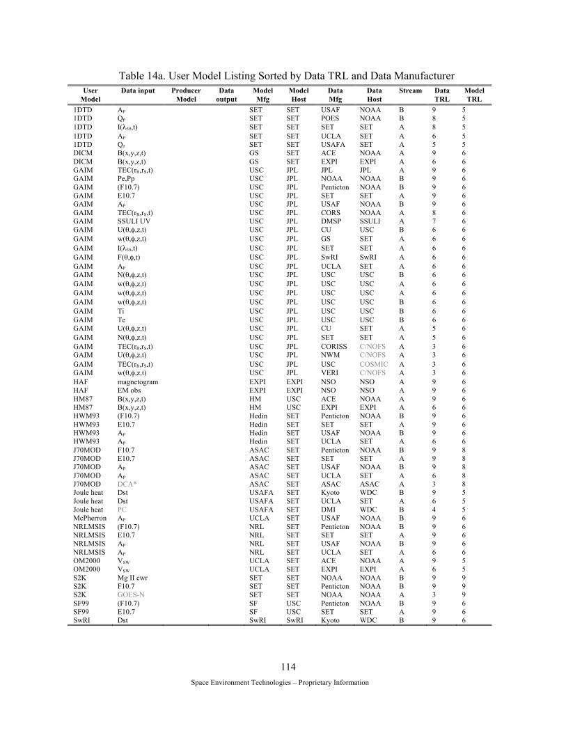
Space Environment Technologies – Proprietary Information
114
Table 14a. User Model Listing Sorted by Data TRL and Data Manufacturer User
Model Data input Producer
Model Data
output Model Mfg
Model Host
Data Mfg
Data Host
Stream Data TRL
Model TRL
1DTD AP SET SET USAF NOAA B 9 5 1DTD QP SET SET POES NOAA B 8 5 1DTD I(λ39,t) SET SET SET SET A 8 5 1DTD AP SET SET UCLA SET A 6 5 1DTD QJ SET SET USAFA SET A 5 5 DICM B(x,y,z,t) GS SET ACE NOAA A 9 6 DICM B(x,y,z,t) GS SET EXPI EXPI A 6 6 GAIM TEC(rR,rS,t) USC JPL JPL JPL A 9 6 GAIM Pe,Pp USC JPL NOAA NOAA B 9 6 GAIM (F10.7) USC JPL Penticton NOAA B 9 6 GAIM E10.7 USC JPL SET SET A 9 6 GAIM AP USC JPL USAF NOAA B 9 6 GAIM TEC(rR,rS,t) USC JPL CORS NOAA A 8 6 GAIM SSULI UV USC JPL DMSP SSULI A 7 6 GAIM U(θ,φ,z,t) USC JPL CU USC B 6 6 GAIM w(θ,φ,z,t) USC JPL GS SET A 6 6 GAIM I(λ39,t) USC JPL SET SET A 6 6 GAIM F(θ,φ,t) USC JPL SwRI SwRI A 6 6 GAIM AP USC JPL UCLA SET A 6 6 GAIM N(θ,φ,z,t) USC JPL USC USC B 6 6 GAIM w(θ,φ,z,t) USC JPL USC USC A 6 6 GAIM w(θ,φ,z,t) USC JPL USC USC A 6 6 GAIM w(θ,φ,z,t) USC JPL USC USC B 6 6 GAIM Ti USC JPL USC USC B 6 6 GAIM Te USC JPL USC USC B 6 6 GAIM U(θ,φ,z,t) USC JPL CU SET A 5 6 GAIM N(θ,φ,z,t) USC JPL SET SET A 5 6 GAIM TEC(rR,rS,t) USC JPL CORISS C/NOFS A 3 6 GAIM U(θ,φ,z,t) USC JPL NWM C/NOFS A 3 6 GAIM TEC(rR,rS,t) USC JPL USC COSMIC A 3 6 GAIM w(θ,φ,z,t) USC JPL VERI C/NOFS A 3 6 HAF magnetogram EXPI EXPI NSO NSO A 9 6 HAF EM obs EXPI EXPI NSO NSO A 9 6 HM87 B(x,y,z,t) HM USC ACE NOAA A 9 6 HM87 B(x,y,z,t) HM USC EXPI EXPI A 6 6 HWM93 (F10.7) Hedin SET Penticton NOAA B 9 6 HWM93 E10.7 Hedin SET SET SET A 9 6 HWM93 AP Hedin SET USAF NOAA B 9 6 HWM93 AP Hedin SET UCLA SET A 6 6 J70MOD F10.7 ASAC SET Penticton NOAA B 9 8 J70MOD E10.7 ASAC SET SET SET A 9 8 J70MOD AP ASAC SET USAF NOAA B 9 8 J70MOD AP ASAC SET UCLA SET A 6 8 J70MOD DCA* ASAC SET ASAC ASAC A 3 8 Joule heat Dst USAFA SET Kyoto WDC B 9 5 Joule heat Dst USAFA SET UCLA SET A 6 5 Joule heat PC USAFA SET DMI WDC B 4 5 McPherron AP UCLA SET USAF NOAA B 9 6 NRLMSIS (F10.7) NRL SET Penticton NOAA B 9 6 NRLMSIS E10.7 NRL SET SET SET A 9 6 NRLMSIS AP NRL SET USAF NOAA B 9 6 NRLMSIS AP NRL SET UCLA SET A 6 6 OM2000 VSW UCLA SET ACE NOAA A 9 5 OM2000 VSW UCLA SET EXPI EXPI A 6 5 S2K Mg II cwr SET SET NOAA NOAA B 9 9 S2K F10.7 SET SET Penticton NOAA B 9 9 S2K GOES-N SET SET NOAA NOAA A 3 9 SF99 (F10.7) SF USC Penticton NOAA B 9 6 SF99 E10.7 SF USC SET SET A 9 6 SwRI Dst SwRI SwRI Kyoto WDC B 9 6

Space Environment Technologies – Proprietary Information
115
Table 14a. User Model Listing Sorted by Data TRL and Data Manufacturer (continued) User
Model Data input
Producer Model
Data output
Model Mfg
Model Host
Data Mfg
Data Host
Stream Data TRL
Model TRL
SwRI (F10.7) SwRI SwRI Penticton NOAA B 9 6 SwRI E10.7 SwRI SwRI SET SET A 9 6 SwRI Kp SwRI SwRI USAF NOAA B 9 6 SwRI Dst SwRI SwRI UCLA SET A 6 6 SwRI PC SwRI SwRI DMI WDC B 4 6 W95 B(x,y,z,t) Weimer USC ACE NOAA A 9 6 W95 B(x,y,z,t) Weimer USC EXPI EXPI A 6 6 *Light gray indicates future capability.
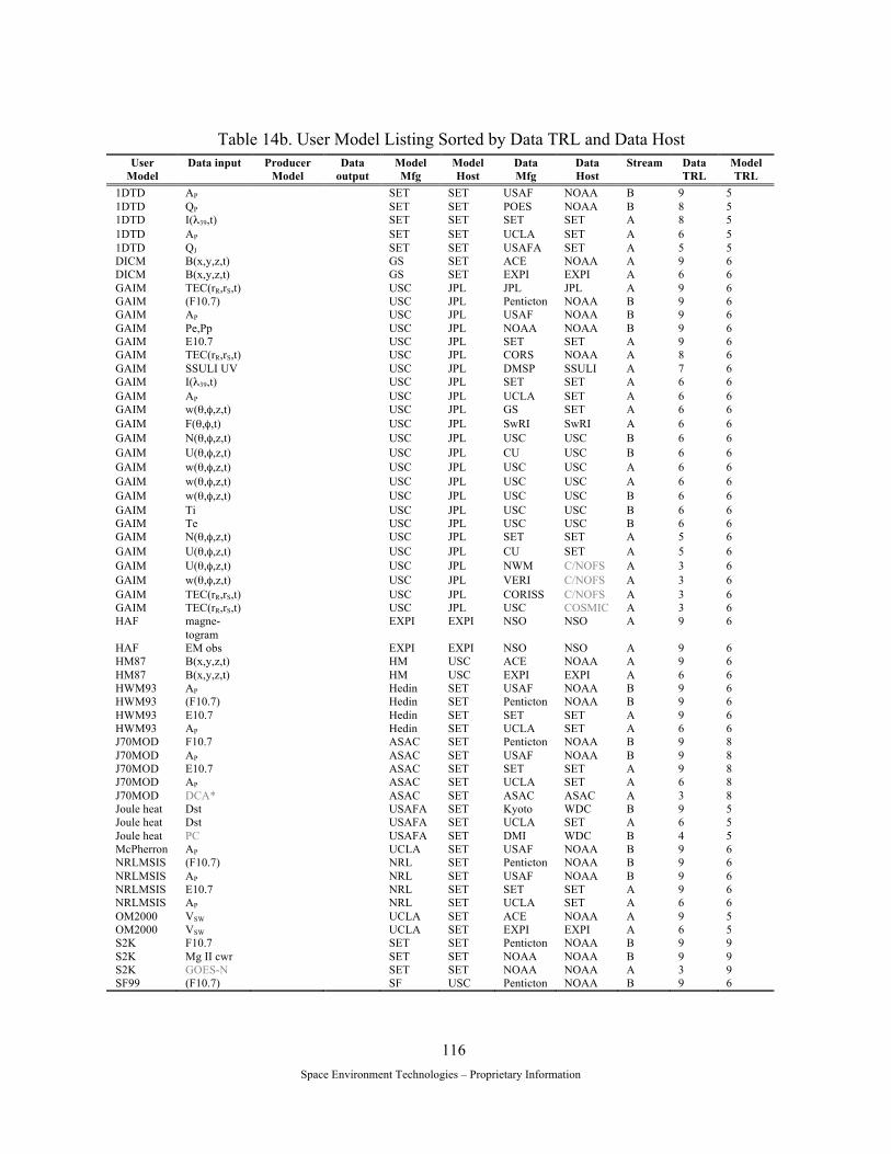
Space Environment Technologies – Proprietary Information
116
Table 14b. User Model Listing Sorted by Data TRL and Data Host
User Model
Data input Producer Model
Data output
Model Mfg
Model Host
Data Mfg
Data Host
Stream Data TRL
Model TRL
1DTD AP SET SET USAF NOAA B 9 5 1DTD QP SET SET POES NOAA B 8 5 1DTD I(λ39,t) SET SET SET SET A 8 5 1DTD AP SET SET UCLA SET A 6 5 1DTD QJ SET SET USAFA SET A 5 5 DICM B(x,y,z,t) GS SET ACE NOAA A 9 6 DICM B(x,y,z,t) GS SET EXPI EXPI A 6 6 GAIM TEC(rR,rS,t) USC JPL JPL JPL A 9 6 GAIM (F10.7) USC JPL Penticton NOAA B 9 6 GAIM AP USC JPL USAF NOAA B 9 6 GAIM Pe,Pp USC JPL NOAA NOAA B 9 6 GAIM E10.7 USC JPL SET SET A 9 6 GAIM TEC(rR,rS,t) USC JPL CORS NOAA A 8 6 GAIM SSULI UV USC JPL DMSP SSULI A 7 6 GAIM I(λ39,t) USC JPL SET SET A 6 6 GAIM AP USC JPL UCLA SET A 6 6 GAIM w(θ,φ,z,t) USC JPL GS SET A 6 6 GAIM F(θ,φ,t) USC JPL SwRI SwRI A 6 6 GAIM N(θ,φ,z,t) USC JPL USC USC B 6 6 GAIM U(θ,φ,z,t) USC JPL CU USC B 6 6 GAIM w(θ,φ,z,t) USC JPL USC USC A 6 6 GAIM w(θ,φ,z,t) USC JPL USC USC A 6 6 GAIM w(θ,φ,z,t) USC JPL USC USC B 6 6 GAIM Ti USC JPL USC USC B 6 6 GAIM Te USC JPL USC USC B 6 6 GAIM N(θ,φ,z,t) USC JPL SET SET A 5 6 GAIM U(θ,φ,z,t) USC JPL CU SET A 5 6 GAIM U(θ,φ,z,t) USC JPL NWM C/NOFS A 3 6 GAIM w(θ,φ,z,t) USC JPL VERI C/NOFS A 3 6 GAIM TEC(rR,rS,t) USC JPL CORISS C/NOFS A 3 6 GAIM TEC(rR,rS,t) USC JPL USC COSMIC A 3 6 HAF magne-
togram EXPI EXPI NSO NSO A 9 6
HAF EM obs EXPI EXPI NSO NSO A 9 6 HM87 B(x,y,z,t) HM USC ACE NOAA A 9 6 HM87 B(x,y,z,t) HM USC EXPI EXPI A 6 6 HWM93 AP Hedin SET USAF NOAA B 9 6 HWM93 (F10.7) Hedin SET Penticton NOAA B 9 6 HWM93 E10.7 Hedin SET SET SET A 9 6 HWM93 AP Hedin SET UCLA SET A 6 6 J70MOD F10.7 ASAC SET Penticton NOAA B 9 8 J70MOD AP ASAC SET USAF NOAA B 9 8 J70MOD E10.7 ASAC SET SET SET A 9 8 J70MOD AP ASAC SET UCLA SET A 6 8 J70MOD DCA* ASAC SET ASAC ASAC A 3 8 Joule heat Dst USAFA SET Kyoto WDC B 9 5 Joule heat Dst USAFA SET UCLA SET A 6 5 Joule heat PC USAFA SET DMI WDC B 4 5 McPherron AP UCLA SET USAF NOAA B 9 6 NRLMSIS (F10.7) NRL SET Penticton NOAA B 9 6 NRLMSIS AP NRL SET USAF NOAA B 9 6 NRLMSIS E10.7 NRL SET SET SET A 9 6 NRLMSIS AP NRL SET UCLA SET A 6 6 OM2000 VSW UCLA SET ACE NOAA A 9 5 OM2000 VSW UCLA SET EXPI EXPI A 6 5 S2K F10.7 SET SET Penticton NOAA B 9 9 S2K Mg II cwr SET SET NOAA NOAA B 9 9 S2K GOES-N SET SET NOAA NOAA A 3 9 SF99 (F10.7) SF USC Penticton NOAA B 9 6

Space Environment Technologies – Proprietary Information
117
Table 14b. User Model Listing Sorted by Data TRL and Data Host (continued) User
Model Data input
Producer Model
Data output
Model Mfg
Model Host
Data Mfg
Data Host
Stream Data TRL
Model TRL
SF99 E10.7 SF USC SET SET A 9 6 SwRI (F10.7) SwRI SwRI Penticton NOAA B 9 6 SwRI Kp SwRI SwRI USAF NOAA B 9 6 SwRI E10.7 SwRI SwRI SET SET A 9 6 SwRI Dst SwRI SwRI Kyoto WDC B 9 6 SwRI Dst SwRI SwRI UCLA SET A 6 6 SwRI PC SwRI SwRI DMI WDC B 4 6 W95 B(x,y,z,t) Weimer USC ACE NOAA A 9 6 W95 B(x,y,z,t) Weimer USC EXPI EXPI A 6 6 *Light gray indicates future capability.

Space Environment Technologies – Proprietary Information
118
Table 14c. User Model Listing Sorted by Model TRL and Model Manufacturer
User Model
Data input Producer Model
Data output
Model Mfg
Model Host
Data Mfg
Data Host
Stream Data TRL
Model TRL
1DTD I(λ39,t) SET SET SET SET A 8 5 1DTD AP SET SET USAF NOAA B 9 5 1DTD AP SET SET UCLA SET A 6 5 1DTD QJ SET SET USAFA SET A 5 5 1DTD QP SET SET POES NOAA B 8 5 DICM B(x,y,z,t) GS SET ACE NOAA A 9 6 DICM B(x,y,z,t) GS SET EXPI EXPI A 6 6 GAIM I(λ39,t) USC JPL SET SET A 6 6 GAIM E10.7 USC JPL SET SET A 9 6 GAIM (F10.7) USC JPL Penticton NOAA B 9 6 GAIM AP USC JPL USAF NOAA B 9 6 GAIM AP USC JPL UCLA SET A 6 6 GAIM N(θ,φ,z,t) USC JPL SET SET A 5 6 GAIM N(θ,φ,z,t) USC JPL USC USC B 6 6 GAIM U(θ,φ,z,t) USC JPL CU SET A 5 6 GAIM U(θ,φ,z,t) USC JPL CU USC B 6 6 GAIM U(θ,φ,z,t) USC JPL NWM C/NOFS A 3 6 GAIM w(θ,φ,z,t) USC JPL GS SET A 6 6 GAIM w(θ,φ,z,t) USC JPL USC USC A 6 6 GAIM w(θ,φ,z,t) USC JPL USC USC A 6 6 GAIM w(θ,φ,z,t) USC JPL USC USC B 6 6 GAIM w(θ,φ,z,t) USC JPL VERI C/NOFS A 3 6 GAIM Pe,Pp USC JPL NOAA NOAA B 9 6 GAIM F(θ,φ,t) USC JPL SwRI SwRI A 6 6 GAIM Ti USC JPL USC USC B 6 6 GAIM Te USC JPL USC USC B 6 6 GAIM SSULI UV USC JPL DMSP SSULI A 7 6 GAIM TEC(rR,rS,t) USC JPL JPL JPL A 9 6 GAIM TEC(rR,rS,t) USC JPL CORISS C/NOFS A 3 6 GAIM TEC(rR,rS,t) USC JPL USC COSMIC A 3 6 GAIM TEC(rR,rS,t) USC JPL CORS NOAA A 8 6 HAF magne-
togram EXPI EXPI NSO NSO A 9 6
HAF EM obs EXPI EXPI NSO NSO A 9 6 HM87 B(x,y,z,t) HM USC ACE NOAA A 9 6 HM87 B(x,y,z,t) HM USC EXPI EXPI A 6 6 HWM93 AP Hedin SET USAF NOAA B 9 6 HWM93 AP Hedin SET UCLA SET A 6 6 HWM93 E10.7 Hedin SET SET SET A 9 6 HWM93 (F10.7) Hedin SET Penticton NOAA B 9 6 J70MOD E10.7 ASAC SET SET SET A 9 8 J70MOD F10.7 ASAC SET Penticton NOAA B 9 8 J70MOD AP ASAC SET USAF NOAA B 9 8 J70MOD AP ASAC SET UCLA SET A 6 8 J70MOD DCA* ASAC SET ASAC ASAC A 3 8 Joule heat Dst USAFA SET Kyoto WDC B 9 5 Joule heat Dst USAFA SET UCLA SET A 6 5 Joule heat PC USAFA SET DMI WDC B 4 5 McPherron AP UCLA SET USAF NOAA B 9 6 NRLMSIS E10.7 NRL SET SET SET A 9 6 NRLMSIS (F10.7) NRL SET Penticton NOAA B 9 6 NRLMSIS AP NRL SET USAF NOAA B 9 6 NRLMSIS AP NRL SET UCLA SET A 6 6 OM2000 VSW UCLA SET ACE NOAA A 9 5 OM2000 VSW UCLA SET EXPI EXPI A 6 5 S2K F10.7 SET SET Penticton NOAA B 9 9 S2K Mg II cwr SET SET NOAA NOAA B 9 9 S2K GOES-N SET SET NOAA NOAA A 3 9 SF99 E10.7 SF USC SET SET A 9 6

Space Environment Technologies – Proprietary Information
119
Table 14c. User Model Listing Sorted by Model TRL and Model Manufacturer (continued) User
Model Data input
Producer Model
Data output
Model Mfg
Model Host
Data Mfg
Data Host
Stream Data TRL
Model TRL
SF99 (F10.7) SF USC Penticton NOAA B 9 6 SwRI Dst SwRI SwRI Kyoto WDC B 9 6 SwRI Dst SwRI SwRI UCLA SET A 6 6 SwRI E10.7 SwRI SwRI SET SET A 9 6 SwRI (F10.7) SwRI SwRI Penticton NOAA B 9 6 SwRI Kp SwRI SwRI USAF NOAA B 9 6 SwRI PC SwRI SwRI DMI WDC B 4 6 W95 B(x,y,z,t) Weimer USC ACE NOAA A 9 6 W95 B(x,y,z,t) Weimer USC EXPI EXPI A 6 6 *Light gray indicates future capability.
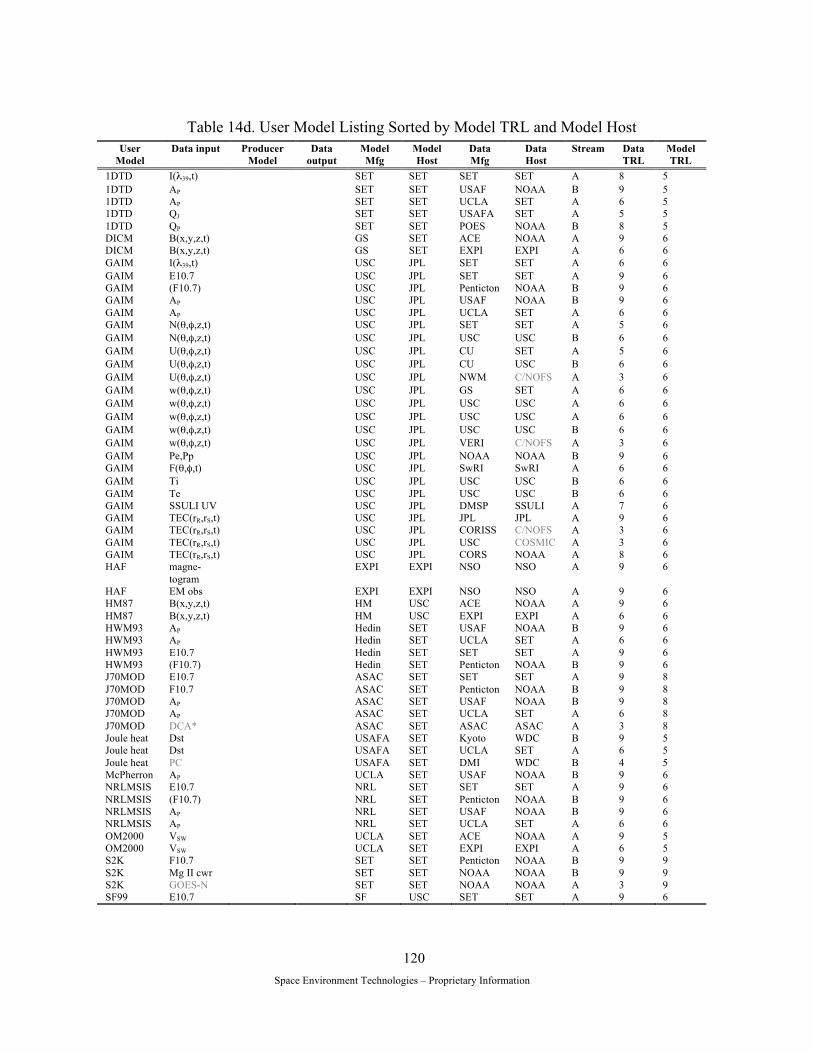
Space Environment Technologies – Proprietary Information
120
Table 14d. User Model Listing Sorted by Model TRL and Model Host
User Model
Data input Producer Model
Data output
Model Mfg
Model Host
Data Mfg
Data Host
Stream Data TRL
Model TRL
1DTD I(λ39,t) SET SET SET SET A 8 5 1DTD AP SET SET USAF NOAA B 9 5 1DTD AP SET SET UCLA SET A 6 5 1DTD QJ SET SET USAFA SET A 5 5 1DTD QP SET SET POES NOAA B 8 5 DICM B(x,y,z,t) GS SET ACE NOAA A 9 6 DICM B(x,y,z,t) GS SET EXPI EXPI A 6 6 GAIM I(λ39,t) USC JPL SET SET A 6 6 GAIM E10.7 USC JPL SET SET A 9 6 GAIM (F10.7) USC JPL Penticton NOAA B 9 6 GAIM AP USC JPL USAF NOAA B 9 6 GAIM AP USC JPL UCLA SET A 6 6 GAIM N(θ,φ,z,t) USC JPL SET SET A 5 6 GAIM N(θ,φ,z,t) USC JPL USC USC B 6 6 GAIM U(θ,φ,z,t) USC JPL CU SET A 5 6 GAIM U(θ,φ,z,t) USC JPL CU USC B 6 6 GAIM U(θ,φ,z,t) USC JPL NWM C/NOFS A 3 6 GAIM w(θ,φ,z,t) USC JPL GS SET A 6 6 GAIM w(θ,φ,z,t) USC JPL USC USC A 6 6 GAIM w(θ,φ,z,t) USC JPL USC USC A 6 6 GAIM w(θ,φ,z,t) USC JPL USC USC B 6 6 GAIM w(θ,φ,z,t) USC JPL VERI C/NOFS A 3 6 GAIM Pe,Pp USC JPL NOAA NOAA B 9 6 GAIM F(θ,φ,t) USC JPL SwRI SwRI A 6 6 GAIM Ti USC JPL USC USC B 6 6 GAIM Te USC JPL USC USC B 6 6 GAIM SSULI UV USC JPL DMSP SSULI A 7 6 GAIM TEC(rR,rS,t) USC JPL JPL JPL A 9 6 GAIM TEC(rR,rS,t) USC JPL CORISS C/NOFS A 3 6 GAIM TEC(rR,rS,t) USC JPL USC COSMIC A 3 6 GAIM TEC(rR,rS,t) USC JPL CORS NOAA A 8 6 HAF magne-
togram EXPI EXPI NSO NSO A 9 6
HAF EM obs EXPI EXPI NSO NSO A 9 6 HM87 B(x,y,z,t) HM USC ACE NOAA A 9 6 HM87 B(x,y,z,t) HM USC EXPI EXPI A 6 6 HWM93 AP Hedin SET USAF NOAA B 9 6 HWM93 AP Hedin SET UCLA SET A 6 6 HWM93 E10.7 Hedin SET SET SET A 9 6 HWM93 (F10.7) Hedin SET Penticton NOAA B 9 6 J70MOD E10.7 ASAC SET SET SET A 9 8 J70MOD F10.7 ASAC SET Penticton NOAA B 9 8 J70MOD AP ASAC SET USAF NOAA B 9 8 J70MOD AP ASAC SET UCLA SET A 6 8 J70MOD DCA* ASAC SET ASAC ASAC A 3 8 Joule heat Dst USAFA SET Kyoto WDC B 9 5 Joule heat Dst USAFA SET UCLA SET A 6 5 Joule heat PC USAFA SET DMI WDC B 4 5 McPherron AP UCLA SET USAF NOAA B 9 6 NRLMSIS E10.7 NRL SET SET SET A 9 6 NRLMSIS (F10.7) NRL SET Penticton NOAA B 9 6 NRLMSIS AP NRL SET USAF NOAA B 9 6 NRLMSIS AP NRL SET UCLA SET A 6 6 OM2000 VSW UCLA SET ACE NOAA A 9 5 OM2000 VSW UCLA SET EXPI EXPI A 6 5 S2K F10.7 SET SET Penticton NOAA B 9 9 S2K Mg II cwr SET SET NOAA NOAA B 9 9 S2K GOES-N SET SET NOAA NOAA A 3 9 SF99 E10.7 SF USC SET SET A 9 6
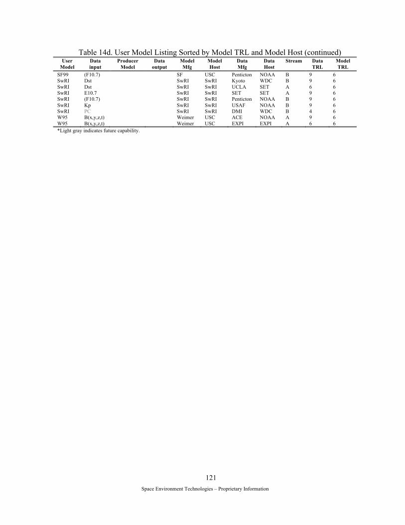
Space Environment Technologies – Proprietary Information
121
Table 14d. User Model Listing Sorted by Model TRL and Model Host (continued) User
Model Data input
Producer Model
Data output
Model Mfg
Model Host
Data Mfg
Data Host
Stream Data TRL
Model TRL
SF99 (F10.7) SF USC Penticton NOAA B 9 6 SwRI Dst SwRI SwRI Kyoto WDC B 9 6 SwRI Dst SwRI SwRI UCLA SET A 6 6 SwRI E10.7 SwRI SwRI SET SET A 9 6 SwRI (F10.7) SwRI SwRI Penticton NOAA B 9 6 SwRI Kp SwRI SwRI USAF NOAA B 9 6 SwRI PC SwRI SwRI DMI WDC B 4 6 W95 B(x,y,z,t) Weimer USC ACE NOAA A 9 6 W95 B(x,y,z,t) Weimer USC EXPI EXPI A 6 6 *Light gray indicates future capability.

Space Environment Technologies – Proprietary Information
122
Table 14e. Producer Model Listing Sorted by Data TRL and Data Manufacturer
User Model
Data input
Producer Model
Data out-put
Model Mfg
Model Host
Data Mfg
Data Host
Stream Data TRL
Model TRL
1DTD N(z,t) SET SET SET SET A 5 5 1DTD ρ(z,t) SET SET SET SET A 5 5 DICM w(θ,φ,z,t) GS SET GS SET A 6 6 GAIM TEC(rR,rS,t) USC JPL USC USC A 6 6 GAIM ne(θ,φ,z,t) USC JPL USC USC A 6 6 HAF B(x,y,z,t) EXPI EXPI EXPI EXPI A 6 6 HAF VSW EXPI EXPI EXPI EXPI A 6 6 HAF nSW EXPI EXPI EXPI EXPI A 6 6 HAF pSW EXPI EXPI EXPI EXPI A 6 6 HM87 w(θ,φ,z,t) HM USC USC USC A 6 6 HWM93 U(θ,φ,z,t) Hedin SET CU USC B 6 6 HWM93 U(θ,φ,z,t) Hedin SET CU SET A 5 6 J70MOD ρ(θ,φ,z,t) ASAC SET ASAC SET A 6 8 Joule heat QJ USAFA SET USAFA SET A 5 5 McPherron AP UCLA SET UCLA SET A 6 6 NRLMSIS N(θ,φ,z,t) NRL USC USC USC B 6 6 NRLMSIS N(θ,φ,z,t) NRL SET SET SET A 5 6 NRLMSIS ρ(θ,φ,z,t) NRL SET SET SET A 5 6 OM2000 Dst UCLA SET UCLA SET A 5 5 S2K E10.7 SET SET SET SET A 9 9 S2K I(λ39,t) SET SET SET SET A 6 9 SF99 w(θ,φ,z,t) SF USC USC USC B 6 6 SwRI F(θ,φ,t) SwRI SwRI SwRI SwRI A 6 6 W95 w(θ,φ,z,t) Weimer USC USC USC A 6 6

Space Environment Technologies – Proprietary Information
123
Table 14f. Producer Model Listing Sorted by Model TRL and Model Manufacturer
User Model
Data input
Producer Model
Data out-put
Model Mfg
Model Host
Data Mfg
Data Host
Stream Data TRL
Model TRL
1DTD N(z,t) SET SET SET SET A 5 5 1DTD ρ(z,t) SET SET SET SET A 5 5 DICM w(θ,φ,z,t) GS SET GS SET A 6 6 GAIM TEC(rR,rS,t) USC JPL USC USC A 6 6 GAIM ne(θ,φ,z,t) USC JPL USC USC A 6 6 HAF B(x,y,z,t) EXPI EXPI EXPI EXPI A 6 6 HAF VSW EXPI EXPI EXPI EXPI A 6 6 HAF nSW EXPI EXPI EXPI EXPI A 6 6 HAF pSW EXPI EXPI EXPI EXPI A 6 6 HM87 w(θ,φ,z,t) HM USC USC USC A 6 6 HWM93 U(θ,φ,z,t) Hedin SET CU SET A 5 6 HWM93 U(θ,φ,z,t) Hedin SET CU USC B 6 6 J70MOD ρ(θ,φ,z,t) ASAC SET ASAC SET A 6 8 Joule heat QJ USAFA SET USAFA SET A 5 5 McPherron AP UCLA SET UCLA SET A 6 6 NRLMSIS N(θ,φ,z,t) NRL SET SET SET A 5 6 NRLMSIS N(θ,φ,z,t) NRL USC USC USC B 6 6 NRLMSIS ρ(θ,φ,z,t) NRL SET SET SET A 5 6 OM2000 Dst UCLA SET UCLA SET A 5 5 S2K I(λ39,t) SET SET SET SET A 6 9 S2K E10.7 SET SET SET SET A 9 9 SF99 w(θ,φ,z,t) SF USC USC USC B 6 6 SwRI F(θ,φ,t) SwRI SwRI SwRI SwRI A 6 6 W95 w(θ,φ,z,t) Weimer USC USC USC A 6 6
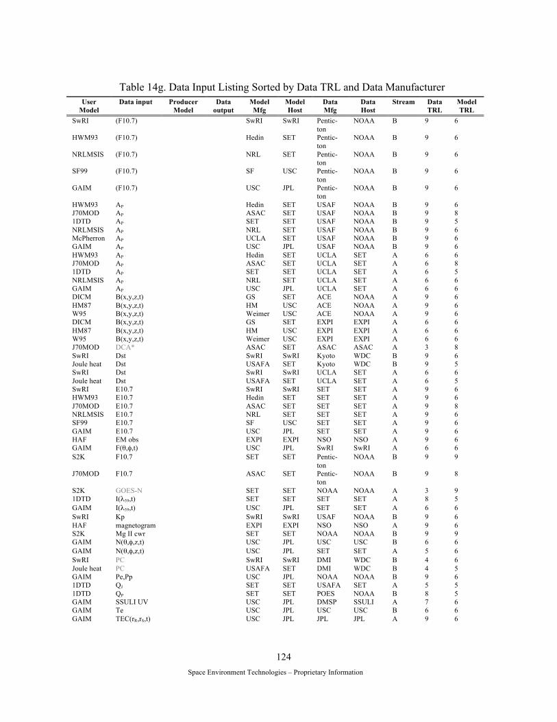
Space Environment Technologies – Proprietary Information
124
Table 14g. Data Input Listing Sorted by Data TRL and Data Manufacturer
User Model
Data input Producer Model
Data output
Model Mfg
Model Host
Data Mfg
Data Host
Stream Data TRL
Model TRL
SwRI (F10.7) SwRI SwRI Pentic-ton
NOAA B 9 6
HWM93 (F10.7) Hedin SET Pentic-ton
NOAA B 9 6
NRLMSIS (F10.7) NRL SET Pentic-ton
NOAA B 9 6
SF99 (F10.7) SF USC Pentic-ton
NOAA B 9 6
GAIM (F10.7) USC JPL Pentic-ton
NOAA B 9 6
HWM93 AP Hedin SET USAF NOAA B 9 6 J70MOD AP ASAC SET USAF NOAA B 9 8 1DTD AP SET SET USAF NOAA B 9 5 NRLMSIS AP NRL SET USAF NOAA B 9 6 McPherron AP UCLA SET USAF NOAA B 9 6 GAIM AP USC JPL USAF NOAA B 9 6 HWM93 AP Hedin SET UCLA SET A 6 6 J70MOD AP ASAC SET UCLA SET A 6 8 1DTD AP SET SET UCLA SET A 6 5 NRLMSIS AP NRL SET UCLA SET A 6 6 GAIM AP USC JPL UCLA SET A 6 6 DICM B(x,y,z,t) GS SET ACE NOAA A 9 6 HM87 B(x,y,z,t) HM USC ACE NOAA A 9 6 W95 B(x,y,z,t) Weimer USC ACE NOAA A 9 6 DICM B(x,y,z,t) GS SET EXPI EXPI A 6 6 HM87 B(x,y,z,t) HM USC EXPI EXPI A 6 6 W95 B(x,y,z,t) Weimer USC EXPI EXPI A 6 6 J70MOD DCA* ASAC SET ASAC ASAC A 3 8 SwRI Dst SwRI SwRI Kyoto WDC B 9 6 Joule heat Dst USAFA SET Kyoto WDC B 9 5 SwRI Dst SwRI SwRI UCLA SET A 6 6 Joule heat Dst USAFA SET UCLA SET A 6 5 SwRI E10.7 SwRI SwRI SET SET A 9 6 HWM93 E10.7 Hedin SET SET SET A 9 6 J70MOD E10.7 ASAC SET SET SET A 9 8 NRLMSIS E10.7 NRL SET SET SET A 9 6 SF99 E10.7 SF USC SET SET A 9 6 GAIM E10.7 USC JPL SET SET A 9 6 HAF EM obs EXPI EXPI NSO NSO A 9 6 GAIM F(θ,φ,t) USC JPL SwRI SwRI A 6 6 S2K F10.7 SET SET Pentic-
ton NOAA B 9 9
J70MOD F10.7 ASAC SET Pentic-ton
NOAA B 9 8
S2K GOES-N SET SET NOAA NOAA A 3 9 1DTD I(λ39,t) SET SET SET SET A 8 5 GAIM I(λ39,t) USC JPL SET SET A 6 6 SwRI Kp SwRI SwRI USAF NOAA B 9 6 HAF magnetogram EXPI EXPI NSO NSO A 9 6 S2K Mg II cwr SET SET NOAA NOAA B 9 9 GAIM N(θ,φ,z,t) USC JPL USC USC B 6 6 GAIM N(θ,φ,z,t) USC JPL SET SET A 5 6 SwRI PC SwRI SwRI DMI WDC B 4 6 Joule heat PC USAFA SET DMI WDC B 4 5 GAIM Pe,Pp USC JPL NOAA NOAA B 9 6 1DTD QJ SET SET USAFA SET A 5 5 1DTD QP SET SET POES NOAA B 8 5 GAIM SSULI UV USC JPL DMSP SSULI A 7 6 GAIM Te USC JPL USC USC B 6 6 GAIM TEC(rR,rS,t) USC JPL JPL JPL A 9 6

Space Environment Technologies – Proprietary Information
125
GAIM TEC(rR,rS,t) USC JPL CORS NOAA A 8 6 GAIM TEC(rR,rS,t) USC JPL CORISS C/NOFS A 3 6 GAIM TEC(rR,rS,t) USC JPL USC COSMIC A 3 6 GAIM Ti USC JPL USC USC B 6 6 GAIM U(θ,φ,z,t) USC JPL CU USC B 6 6
Table 14g. Data Input Listing Sorted by Data TRL and Data Manufacturer (continued)
User Model
Data input
Producer Model
Data output
Model Mfg
Model Host
Data Mfg
Data Host
Stream Data TRL
Model TRL
GAIM U(θ,φ,z,t) USC JPL CU SET A 5 6 GAIM U(θ,φ,z,t) USC JPL NWM C/NOFS A 3 6 OM2000 VSW UCLA SET ACE NOAA A 9 5 OM2000 VSW UCLA SET EXPI EXPI A 6 5 GAIM w(θ,φ,z,t) USC JPL GS SET A 6 6 GAIM w(θ,φ,z,t) USC JPL USC USC A 6 6 GAIM w(θ,φ,z,t) USC JPL USC USC A 6 6 GAIM w(θ,φ,z,t) USC JPL USC USC B 6 6 GAIM w(θ,φ,z,t) USC JPL VERI C/NOFS A 3 6 *Light gray indicates future capability.

Space Environment Technologies – Proprietary Information
126
Table 14h. Data Output Listing Sorted by Data TRL and Data Manufacturer
User Model
Data input
Producer Model
Data out-put
Model Mfg
Model Host
Data Mfg
Data Host
Stream Data TRL
Model TRL
J70MOD ρ(θ,φ,z,t) ASAC SET ASAC SET A 6 8 NRLMSIS ρ(θ,φ,z,t) NRL SET SET SET A 5 6 1DTD ρ(z,t) SET SET SET SET A 5 5 McPherron AP UCLA SET UCLA SET A 6 6 HAF B(x,y,z,t) EXPI EXPI EXPI EXPI A 6 6 OM2000 Dst UCLA SET UCLA SET A 5 5 S2K E10.7 SET SET SET SET A 9 9 SwRI F(θ,φ,t) SwRI SwRI SwRI SwRI A 6 6 S2K I(λ39,t) SET SET SET SET A 6 9 NRLMSIS N(θ,φ,z,t) NRL USC USC USC B 6 6 NRLMSIS N(θ,φ,z,t) NRL SET SET SET A 5 6 1DTD N(z,t) SET SET SET SET A 5 5 GAIM ne(θ,φ,z,t) USC JPL USC USC A 6 6 HAF nSW EXPI EXPI EXPI EXPI A 6 6 HAF pSW EXPI EXPI EXPI EXPI A 6 6 Joule heat QJ USAFA SET USAFA SET A 5 5 GAIM TEC(rR,rS,t) USC JPL USC USC A 6 6 HWM93 U(θ,φ,z,t) Hedin SET CU USC B 6 6 HWM93 U(θ,φ,z,t) Hedin SET CU SET A 5 6 HAF VSW EXPI EXPI EXPI EXPI A 6 6 DICM w(θ,φ,z,t) GS SET GS SET A 6 6 HM87 w(θ,φ,z,t) HM USC USC USC A 6 6 W95 w(θ,φ,z,t) Weimer USC USC USC A 6 6 SF99 w(θ,φ,z,t) SF USC USC USC B 6 6

Space Environment Technologies – Proprietary Information
127
Table 14i. Data Input Listing Sorted by Data Stream and Data TRL
User Model
Data input Producer Model
Data output
Model Mfg
Model Host
Data Mfg
Data Host
Stream Data TRL
Model TRL
SwRI (F10.7) SwRI SwRI Penticton NOAA B 9 6 HWM93 (F10.7) Hedin SET Penticton NOAA B 9 6 NRLMSIS (F10.7) NRL SET Penticton NOAA B 9 6 SF99 (F10.7) SF USC Penticton NOAA B 9 6 GAIM (F10.7) USC JPL Penticton NOAA B 9 6 HWM93 AP Hedin SET UCLA SET A 6 6 J70MOD AP ASAC SET UCLA SET A 6 8 1DTD AP SET SET UCLA SET A 6 5 NRLMSIS AP NRL SET UCLA SET A 6 6 GAIM AP USC JPL UCLA SET A 6 6 HWM93 AP Hedin SET USAF NOAA B 9 6 J70MOD AP ASAC SET USAF NOAA B 9 8 1DTD AP SET SET USAF NOAA B 9 5 NRLMSIS AP NRL SET USAF NOAA B 9 6 McPherron AP UCLA SET USAF NOAA B 9 6 GAIM AP USC JPL USAF NOAA B 9 6 DICM B(x,y,z,t) GS SET ACE NOAA A 9 6 HM87 B(x,y,z,t) HM USC ACE NOAA A 9 6 W95 B(x,y,z,t) Weimer USC ACE NOAA A 9 6 DICM B(x,y,z,t) GS SET EXPI EXPI A 6 6 HM87 B(x,y,z,t) HM USC EXPI EXPI A 6 6 W95 B(x,y,z,t) Weimer USC EXPI EXPI A 6 6 J70MOD DCA* ASAC SET ASAC ASAC A 3 8 SwRI Dst SwRI SwRI UCLA SET A 6 6 Joule heat Dst USAFA SET UCLA SET A 6 5 SwRI Dst SwRI SwRI Kyoto WDC B 9 6 Joule heat Dst USAFA SET Kyoto WDC B 9 5 SwRI E10.7 SwRI SwRI SET SET A 9 6 HWM93 E10.7 Hedin SET SET SET A 9 6 J70MOD E10.7 ASAC SET SET SET A 9 8 NRLMSIS E10.7 NRL SET SET SET A 9 6 SF99 E10.7 SF USC SET SET A 9 6 GAIM E10.7 USC JPL SET SET A 9 6 HAF EM obs EXPI EXPI NSO NSO A 9 6 GAIM F(θ,φ,t) USC JPL SwRI SwRI A 6 6 S2K F10.7 SET SET Penticton NOAA B 9 9 J70MOD F10.7 ASAC SET Penticton NOAA B 9 8 S2K GOES-N SET SET NOAA NOAA A 3 9 1DTD I(λ39,t) SET SET SET SET A 8 5 GAIM I(λ39,t) USC JPL SET SET A 6 6 SwRI Kp SwRI SwRI USAF NOAA B 9 6 HAF magnetogram EXPI EXPI NSO NSO A 9 6 S2K Mg II cwr SET SET NOAA NOAA B 9 9 GAIM N(θ,φ,z,t) USC JPL SET SET A 5 6 GAIM N(θ,φ,z,t) USC JPL USC USC B 6 6 SwRI PC SwRI SwRI DMI WDC B 4 6 Joule heat PC USAFA SET DMI WDC B 4 5 GAIM Pe,Pp USC JPL NOAA NOAA B 9 6 1DTD QJ SET SET USAFA SET A 5 5 1DTD QP SET SET POES NOAA B 8 5 GAIM SSULI UV USC JPL DMSP SSULI A 7 6 GAIM Te USC JPL USC USC B 6 6 GAIM TEC(rR,rS,t) USC JPL JPL JPL A 9 6 GAIM TEC(rR,rS,t) USC JPL CORS NOAA A 8 6 GAIM TEC(rR,rS,t) USC JPL CORISS C/NOFS A 3 6 GAIM TEC(rR,rS,t) USC JPL USC COSMIC A 3 6 GAIM Ti USC JPL USC USC B 6 6 GAIM U(θ,φ,z,t) USC JPL CU SET A 5 6 *Light gray indicates future capability.
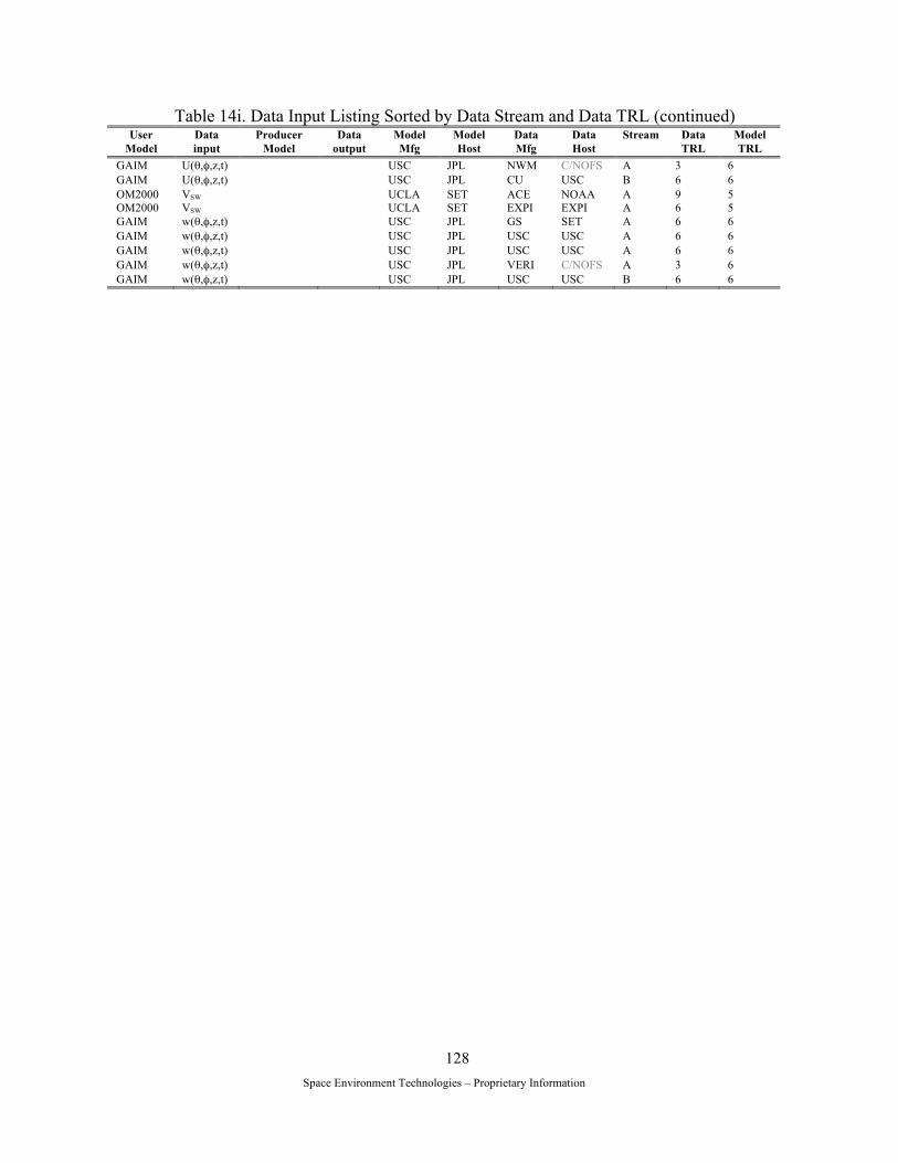
Space Environment Technologies – Proprietary Information
128
Table 14i. Data Input Listing Sorted by Data Stream and Data TRL (continued) User
Model Data input
Producer Model
Data output
Model Mfg
Model Host
Data Mfg
Data Host
Stream Data TRL
Model TRL
GAIM U(θ,φ,z,t) USC JPL NWM C/NOFS A 3 6 GAIM U(θ,φ,z,t) USC JPL CU USC B 6 6 OM2000 VSW UCLA SET ACE NOAA A 9 5 OM2000 VSW UCLA SET EXPI EXPI A 6 5 GAIM w(θ,φ,z,t) USC JPL GS SET A 6 6 GAIM w(θ,φ,z,t) USC JPL USC USC A 6 6 GAIM w(θ,φ,z,t) USC JPL USC USC A 6 6 GAIM w(θ,φ,z,t) USC JPL VERI C/NOFS A 3 6 GAIM w(θ,φ,z,t) USC JPL USC USC B 6 6

Space Environment Technologies – Proprietary Information
129
Table 14j. Data Output Listing Sorted by Data Stream and Data TRL
User Model
Data input
Producer Model
Data out-put
Model Mfg
Model Host
Data Mfg
Data Host
Stream Data TRL
Model TRL
J70MOD ρ(θ,φ,z,t) ASAC SET ASAC SET A 6 8 NRLMSIS ρ(θ,φ,z,t) NRL SET SET SET A 5 6 1DTD ρ(z,t) SET SET SET SET A 5 5 McPherron AP UCLA SET UCLA SET A 6 6 HAF B(x,y,z,t) EXPI EXPI EXPI EXPI A 6 6 OM2000 Dst UCLA SET UCLA SET A 5 5 S2K E10.7 SET SET SET SET A 9 9 SwRI F(θ,φ,t) SwRI SwRI SwRI SwRI A 6 6 S2K I(λ39,t) SET SET SET SET A 6 9 NRLMSIS N(θ,φ,z,t) NRL SET SET SET A 5 6 NRLMSIS N(θ,φ,z,t) NRL USC USC USC B 6 6 1DTD N(z,t) SET SET SET SET A 5 5 GAIM ne(θ,φ,z,t) USC JPL USC USC A 6 6 HAF nSW EXPI EXPI EXPI EXPI A 6 6 HAF pSW EXPI EXPI EXPI EXPI A 6 6 Joule heat QJ USAFA SET USAFA SET A 5 5 GAIM TEC(rR,rS,t) USC JPL USC USC A 6 6 HWM93 U(θ,φ,z,t) Hedin SET CU SET A 5 6 HWM93 U(θ,φ,z,t) Hedin SET CU USC B 6 6 HAF VSW EXPI EXPI EXPI EXPI A 6 6 DICM w(θ,φ,z,t) GS SET GS SET A 6 6 HM87 w(θ,φ,z,t) HM USC USC USC A 6 6 W95 w(θ,φ,z,t) Weimer USC USC USC A 6 6 SF99 w(θ,φ,z,t) SF USC USC USC B 6 6

Space Environment Technologies – Proprietary Information
130
Table 14k. Data Input Listing Sorted by Data Stream and Data Manufacturer
User Model
Data input Producer Model
Data output
Model Mfg
Model Host
Data Mfg
Data Host
Stream Data TRL
Model TRL
SwRI (F10.7) SwRI SwRI Penticton NOAA B 9 6 HWM93 (F10.7) Hedin SET Penticton NOAA B 9 6 NRLMSIS (F10.7) NRL SET Penticton NOAA B 9 6 SF99 (F10.7) SF USC Penticton NOAA B 9 6 GAIM (F10.7) USC JPL Penticton NOAA B 9 6 HWM93 AP Hedin SET UCLA SET A 6 6 J70MOD AP ASAC SET UCLA SET A 6 8 1DTD AP SET SET UCLA SET A 6 5 NRLMSIS AP NRL SET UCLA SET A 6 6 GAIM AP USC JPL UCLA SET A 6 6 HWM93 AP Hedin SET USAF NOAA B 9 6 J70MOD AP ASAC SET USAF NOAA B 9 8 1DTD AP SET SET USAF NOAA B 9 5 NRLMSIS AP NRL SET USAF NOAA B 9 6 McPherron AP UCLA SET USAF NOAA B 9 6 GAIM AP USC JPL USAF NOAA B 9 6 DICM B(x,y,z,t) GS SET EXPI EXPI A 6 6 HM87 B(x,y,z,t) HM USC EXPI EXPI A 6 6 W95 B(x,y,z,t) Weimer USC EXPI EXPI A 6 6 DICM B(x,y,z,t) GS SET ACE NOAA A 9 6 HM87 B(x,y,z,t) HM USC ACE NOAA A 9 6 W95 B(x,y,z,t) Weimer USC ACE NOAA A 9 6 J70MOD DCA* ASAC SET ASAC ASAC A 3 8 SwRI Dst SwRI SwRI UCLA SET A 6 6 Joule heat Dst USAFA SET UCLA SET A 6 5 SwRI Dst SwRI SwRI Kyoto WDC B 9 6 Joule heat Dst USAFA SET Kyoto WDC B 9 5 SwRI E10.7 SwRI SwRI SET SET A 9 6 HWM93 E10.7 Hedin SET SET SET A 9 6 J70MOD E10.7 ASAC SET SET SET A 9 8 NRLMSIS E10.7 NRL SET SET SET A 9 6 SF99 E10.7 SF USC SET SET A 9 6 GAIM E10.7 USC JPL SET SET A 9 6 HAF EM obs EXPI EXPI NSO NSO A 9 6 GAIM F(θ,φ,t) USC JPL SwRI SwRI A 6 6 S2K F10.7 SET SET Penticton NOAA B 9 9 J70MOD F10.7 ASAC SET Penticton NOAA B 9 8 S2K GOES-N SET SET NOAA NOAA A 3 9 1DTD I(λ39,t) SET SET SET SET A 8 5 GAIM I(λ39,t) USC JPL SET SET A 6 6 SwRI Kp SwRI SwRI USAF NOAA B 9 6 HAF magnetogram EXPI EXPI NSO NSO A 9 6 S2K Mg II cwr SET SET NOAA NOAA B 9 9 GAIM N(θ,φ,z,t) USC JPL SET SET A 5 6 GAIM N(θ,φ,z,t) USC JPL USC USC B 6 6 SwRI PC SwRI SwRI DMI WDC B 4 6 Joule heat PC USAFA SET DMI WDC B 4 5 GAIM Pe,Pp USC JPL NOAA NOAA B 9 6 1DTD QJ SET SET USAFA SET A 5 5 1DTD QP SET SET POES NOAA B 8 5 GAIM SSULI UV USC JPL DMSP SSULI A 7 6 GAIM Te USC JPL USC USC B 6 6 GAIM TEC(rR,rS,t) USC JPL USC COSMIC A 3 6 GAIM TEC(rR,rS,t) USC JPL JPL JPL A 9 6 GAIM TEC(rR,rS,t) USC JPL CORS NOAA A 8 6 GAIM TEC(rR,rS,t) USC JPL CORISS C/NOFS A 3 6 GAIM Ti USC JPL USC USC B 6 6 GAIM U(θ,φ,z,t) USC JPL NWM C/NOFS A 3 6

Space Environment Technologies – Proprietary Information
131
Table 14k. Data Input Listing Sorted by Data Stream and Data Manufacturer (continued) User
Model Data input
Producer Model
Data output
Model Mfg
Model Host
Data Mfg
Data Host
Stream Data TRL
Model TRL
GAIM U(θ,φ,z,t) USC JPL CU SET A 5 6 GAIM U(θ,φ,z,t) USC JPL CU USC B 6 6 OM2000 VSW UCLA SET EXPI EXPI A 6 5 OM2000 VSW UCLA SET ACE NOAA A 9 5 GAIM w(θ,φ,z,t) USC JPL VERI C/NOFS A 3 6 GAIM w(θ,φ,z,t) USC JPL USC USC A 6 6 GAIM w(θ,φ,z,t) USC JPL USC USC A 6 6 GAIM w(θ,φ,z,t) USC JPL GS SET A 6 6 GAIM w(θ,φ,z,t) USC JPL USC USC B 6 6 *Light gray indicates future capability.
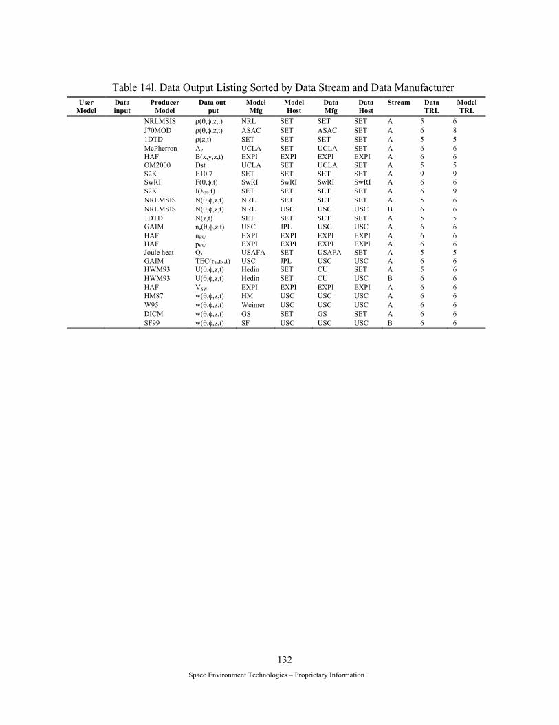
Space Environment Technologies – Proprietary Information
132
Table 14l. Data Output Listing Sorted by Data Stream and Data Manufacturer
User Model
Data input
Producer Model
Data out-put
Model Mfg
Model Host
Data Mfg
Data Host
Stream Data TRL
Model TRL
NRLMSIS ρ(θ,φ,z,t) NRL SET SET SET A 5 6 J70MOD ρ(θ,φ,z,t) ASAC SET ASAC SET A 6 8 1DTD ρ(z,t) SET SET SET SET A 5 5 McPherron AP UCLA SET UCLA SET A 6 6 HAF B(x,y,z,t) EXPI EXPI EXPI EXPI A 6 6 OM2000 Dst UCLA SET UCLA SET A 5 5 S2K E10.7 SET SET SET SET A 9 9 SwRI F(θ,φ,t) SwRI SwRI SwRI SwRI A 6 6 S2K I(λ39,t) SET SET SET SET A 6 9 NRLMSIS N(θ,φ,z,t) NRL SET SET SET A 5 6 NRLMSIS N(θ,φ,z,t) NRL USC USC USC B 6 6 1DTD N(z,t) SET SET SET SET A 5 5 GAIM ne(θ,φ,z,t) USC JPL USC USC A 6 6 HAF nSW EXPI EXPI EXPI EXPI A 6 6 HAF pSW EXPI EXPI EXPI EXPI A 6 6 Joule heat QJ USAFA SET USAFA SET A 5 5 GAIM TEC(rR,rS,t) USC JPL USC USC A 6 6 HWM93 U(θ,φ,z,t) Hedin SET CU SET A 5 6 HWM93 U(θ,φ,z,t) Hedin SET CU USC B 6 6 HAF VSW EXPI EXPI EXPI EXPI A 6 6 HM87 w(θ,φ,z,t) HM USC USC USC A 6 6 W95 w(θ,φ,z,t) Weimer USC USC USC A 6 6 DICM w(θ,φ,z,t) GS SET GS SET A 6 6 SF99 w(θ,φ,z,t) SF USC USC USC B 6 6

Space Environment Technologies – Proprietary Information
133
Table 14m. Data Input Listing Sorted by Data Stream and Data Host
User Model
Data input Producer Model
Data output
Model Mfg
Model Host
Data Mfg
Data Host
Stream Data TRL
Model TRL
SwRI (F10.7) SwRI SwRI Penticton NOAA B 9 6 HWM93 (F10.7) Hedin SET Penticton NOAA B 9 6 NRLMSIS (F10.7) NRL SET Penticton NOAA B 9 6 SF99 (F10.7) SF USC Penticton NOAA B 9 6 GAIM (F10.7) USC JPL Penticton NOAA B 9 6 HWM93 AP Hedin SET UCLA SET A 6 6 J70MOD AP ASAC SET UCLA SET A 6 8 1DTD AP SET SET UCLA SET A 6 5 NRLMSIS AP NRL SET UCLA SET A 6 6 GAIM AP USC JPL UCLA SET A 6 6 HWM93 AP Hedin SET USAF NOAA B 9 6 J70MOD AP ASAC SET USAF NOAA B 9 8 1DTD AP SET SET USAF NOAA B 9 5 NRLMSIS AP NRL SET USAF NOAA B 9 6 McPherron AP UCLA SET USAF NOAA B 9 6 GAIM AP USC JPL USAF NOAA B 9 6 DICM B(x,y,z,t) GS SET ACE NOAA A 9 6 HM87 B(x,y,z,t) HM USC ACE NOAA A 9 6 W95 B(x,y,z,t) Weimer USC ACE NOAA A 9 6 DICM B(x,y,z,t) GS SET EXPI EXPI A 6 6 HM87 B(x,y,z,t) HM USC EXPI EXPI A 6 6 W95 B(x,y,z,t) Weimer USC EXPI EXPI A 6 6 J70MOD DCA* ASAC SET ASAC ASAC A 3 8 SwRI Dst SwRI SwRI UCLA SET A 6 6 Joule heat Dst USAFA SET UCLA SET A 6 5 SwRI Dst SwRI SwRI Kyoto WDC B 9 6 Joule heat Dst USAFA SET Kyoto WDC B 9 5 SwRI E10.7 SwRI SwRI SET SET A 9 6 HWM93 E10.7 Hedin SET SET SET A 9 6 J70MOD E10.7 ASAC SET SET SET A 9 8 NRLMSIS E10.7 NRL SET SET SET A 9 6 SF99 E10.7 SF USC SET SET A 9 6 GAIM E10.7 USC JPL SET SET A 9 6 HAF EM obs EXPI EXPI NSO NSO A 9 6 GAIM F(θ,φ,t) USC JPL SwRI SwRI A 6 6 S2K F10.7 SET SET Penticton NOAA B 9 9 J70MOD F10.7 ASAC SET Penticton NOAA B 9 8 S2K GOES-N SET SET NOAA NOAA A 3 9 1DTD I(λ39,t) SET SET SET SET A 8 5 GAIM I(λ39,t) USC JPL SET SET A 6 6 SwRI Kp SwRI SwRI USAF NOAA B 9 6 HAF magnetogram EXPI EXPI NSO NSO A 9 6 S2K Mg II cwr SET SET NOAA NOAA B 9 9 GAIM N(θ,φ,z,t) USC JPL SET SET A 5 6 GAIM N(θ,φ,z,t) USC JPL USC USC B 6 6 SwRI PC SwRI SwRI DMI WDC B 4 6 Joule heat PC USAFA SET DMI WDC B 4 5 GAIM Pe,Pp USC JPL NOAA NOAA B 9 6 1DTD QJ SET SET USAFA SET A 5 5 1DTD QP SET SET POES NOAA B 8 5 GAIM SSULI UV USC JPL DMSP SSULI A 7 6 GAIM Te USC JPL USC USC B 6 6 GAIM TEC(rR,rS,t) USC JPL CORS NOAA A 8 6 GAIM TEC(rR,rS,t) USC JPL JPL JPL A 9 6 GAIM TEC(rR,rS,t) USC JPL USC COSMIC A 3 6 GAIM TEC(rR,rS,t) USC JPL CORISS C/NOFS A 3 6 GAIM Ti USC JPL USC USC B 6 6 GAIM U(θ,φ,z,t) USC JPL CU SET A 5 6

Space Environment Technologies – Proprietary Information
134
Table 14m. Data Input Listing Sorted by Data Stream and Data Host (continued) User
Model Data input
Producer Model
Data output
Model Mfg
Model Host
Data Mfg
Data Host
Stream Data TRL
Model TRL
GAIM U(θ,φ,z,t) USC JPL NWM C/NOFS A 3 6 GAIM U(θ,φ,z,t) USC JPL CU USC B 6 6 OM2000 VSW UCLA SET ACE NOAA A 9 5 OM2000 VSW UCLA SET EXPI EXPI A 6 5 GAIM w(θ,φ,z,t) USC JPL USC USC A 6 6 GAIM w(θ,φ,z,t) USC JPL USC USC A 6 6 GAIM w(θ,φ,z,t) USC JPL GS SET A 6 6 GAIM w(θ,φ,z,t) USC JPL VERI C/NOFS A 3 6 GAIM w(θ,φ,z,t) USC JPL USC USC B 6 6 *Light gray indicates future capability.

Space Environment Technologies – Proprietary Information
135
Table 14n. Data Output Listing Sorted by Data Stream and Data Host
User Model
Data input
Producer Model
Data out-put
Model Mfg
Model Host
Data Mfg
Data Host
Stream Data TRL
Model TRL
J70MOD ρ(θ,φ,z,t) ASAC SET ASAC SET A 6 8 NRLMSIS ρ(θ,φ,z,t) NRL SET SET SET A 5 6 1DTD ρ(z,t) SET SET SET SET A 5 5 McPherron AP UCLA SET UCLA SET A 6 6 HAF B(x,y,z,t) EXPI EXPI EXPI EXPI A 6 6 OM2000 Dst UCLA SET UCLA SET A 5 5 S2K E10.7 SET SET SET SET A 9 9 SwRI F(θ,φ,t) SwRI SwRI SwRI SwRI A 6 6 S2K I(λ39,t) SET SET SET SET A 6 9 NRLMSIS N(θ,φ,z,t) NRL SET SET SET A 5 6 NRLMSIS N(θ,φ,z,t) NRL USC USC USC B 6 6 1DTD N(z,t) SET SET SET SET A 5 5 GAIM ne(θ,φ,z,t) USC JPL USC USC A 6 6 HAF nSW EXPI EXPI EXPI EXPI A 6 6 HAF pSW EXPI EXPI EXPI EXPI A 6 6 Joule heat QJ USAFA SET USAFA SET A 5 5 GAIM TEC(rR,rS,t) USC JPL USC USC A 6 6 HWM93 U(θ,φ,z,t) Hedin SET CU SET A 5 6 HWM93 U(θ,φ,z,t) Hedin SET CU USC B 6 6 HAF VSW EXPI EXPI EXPI EXPI A 6 6 HM87 w(θ,φ,z,t) HM USC USC USC A 6 6 W95 w(θ,φ,z,t) Weimer USC USC USC A 6 6 DICM w(θ,φ,z,t) GS SET GS SET A 6 6 SF99 w(θ,φ,z,t) SF USC USC USC B 6 6
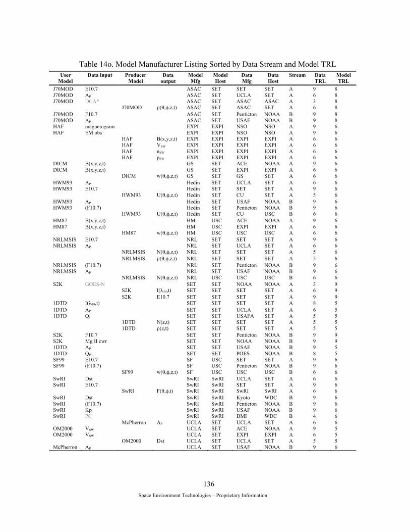
Space Environment Technologies – Proprietary Information
136
Table 14o. Model Manufacturer Listing Sorted by Data Stream and Model TRL
User Model
Data input Producer Model
Data output
Model Mfg
Model Host
Data Mfg
Data Host
Stream Data TRL
Model TRL
J70MOD E10.7 ASAC SET SET SET A 9 8 J70MOD AP ASAC SET UCLA SET A 6 8 J70MOD DCA* ASAC SET ASAC ASAC A 3 8 J70MOD ρ(θ,φ,z,t) ASAC SET ASAC SET A 6 8 J70MOD F10.7 ASAC SET Penticton NOAA B 9 8 J70MOD AP ASAC SET USAF NOAA B 9 8 HAF magnetogram EXPI EXPI NSO NSO A 9 6 HAF EM obs EXPI EXPI NSO NSO A 9 6 HAF B(x,y,z,t) EXPI EXPI EXPI EXPI A 6 6 HAF VSW EXPI EXPI EXPI EXPI A 6 6 HAF nSW EXPI EXPI EXPI EXPI A 6 6 HAF pSW EXPI EXPI EXPI EXPI A 6 6 DICM B(x,y,z,t) GS SET ACE NOAA A 9 6 DICM B(x,y,z,t) GS SET EXPI EXPI A 6 6 DICM w(θ,φ,z,t) GS SET GS SET A 6 6 HWM93 AP Hedin SET UCLA SET A 6 6 HWM93 E10.7 Hedin SET SET SET A 9 6 HWM93 U(θ,φ,z,t) Hedin SET CU SET A 5 6 HWM93 AP Hedin SET USAF NOAA B 9 6 HWM93 (F10.7) Hedin SET Penticton NOAA B 9 6 HWM93 U(θ,φ,z,t) Hedin SET CU USC B 6 6 HM87 B(x,y,z,t) HM USC ACE NOAA A 9 6 HM87 B(x,y,z,t) HM USC EXPI EXPI A 6 6 HM87 w(θ,φ,z,t) HM USC USC USC A 6 6 NRLMSIS E10.7 NRL SET SET SET A 9 6 NRLMSIS AP NRL SET UCLA SET A 6 6 NRLMSIS N(θ,φ,z,t) NRL SET SET SET A 5 6 NRLMSIS ρ(θ,φ,z,t) NRL SET SET SET A 5 6 NRLMSIS (F10.7) NRL SET Penticton NOAA B 9 6 NRLMSIS AP NRL SET USAF NOAA B 9 6 NRLMSIS N(θ,φ,z,t) NRL USC USC USC B 6 6 S2K GOES-N SET SET NOAA NOAA A 3 9 S2K I(λ39,t) SET SET SET SET A 6 9 S2K E10.7 SET SET SET SET A 9 9 1DTD I(λ39,t) SET SET SET SET A 8 5 1DTD AP SET SET UCLA SET A 6 5 1DTD QJ SET SET USAFA SET A 5 5 1DTD N(z,t) SET SET SET SET A 5 5 1DTD ρ(z,t) SET SET SET SET A 5 5 S2K F10.7 SET SET Penticton NOAA B 9 9 S2K Mg II cwr SET SET NOAA NOAA B 9 9 1DTD AP SET SET USAF NOAA B 9 5 1DTD QP SET SET POES NOAA B 8 5 SF99 E10.7 SF USC SET SET A 9 6 SF99 (F10.7) SF USC Penticton NOAA B 9 6 SF99 w(θ,φ,z,t) SF USC USC USC B 6 6 SwRI Dst SwRI SwRI UCLA SET A 6 6 SwRI E10.7 SwRI SwRI SET SET A 9 6 SwRI F(θ,φ,t) SwRI SwRI SwRI SwRI A 6 6 SwRI Dst SwRI SwRI Kyoto WDC B 9 6 SwRI (F10.7) SwRI SwRI Penticton NOAA B 9 6 SwRI Kp SwRI SwRI USAF NOAA B 9 6 SwRI PC SwRI SwRI DMI WDC B 4 6 McPherron AP UCLA SET UCLA SET A 6 6 OM2000 VSW UCLA SET ACE NOAA A 9 5 OM2000 VSW UCLA SET EXPI EXPI A 6 5 OM2000 Dst UCLA SET UCLA SET A 5 5 McPherron AP UCLA SET USAF NOAA B 9 6
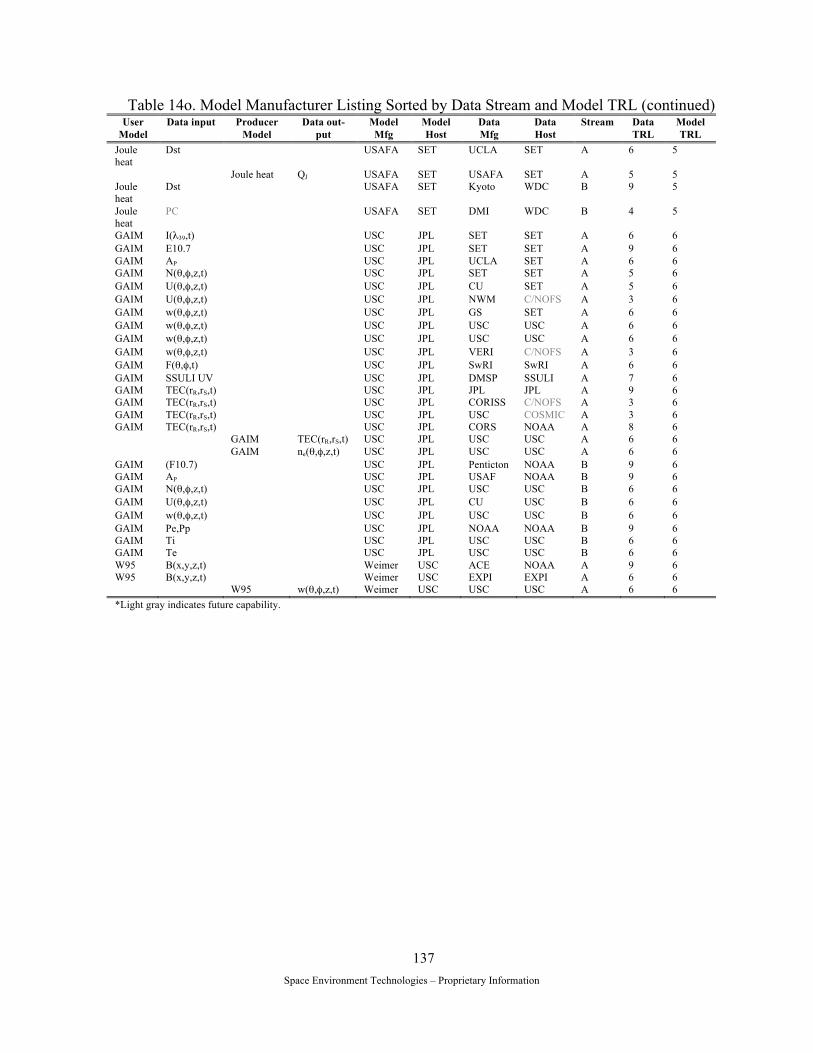
Space Environment Technologies – Proprietary Information
137
Table 14o. Model Manufacturer Listing Sorted by Data Stream and Model TRL (continued) User
Model Data input Producer
Model Data out-
put Model Mfg
Model Host
Data Mfg
Data Host
Stream Data TRL
Model TRL
Joule heat
Dst USAFA SET UCLA SET A 6 5
Joule heat QJ USAFA SET USAFA SET A 5 5 Joule heat
Dst USAFA SET Kyoto WDC B 9 5
Joule heat
PC USAFA SET DMI WDC B 4 5
GAIM I(λ39,t) USC JPL SET SET A 6 6 GAIM E10.7 USC JPL SET SET A 9 6 GAIM AP USC JPL UCLA SET A 6 6 GAIM N(θ,φ,z,t) USC JPL SET SET A 5 6 GAIM U(θ,φ,z,t) USC JPL CU SET A 5 6 GAIM U(θ,φ,z,t) USC JPL NWM C/NOFS A 3 6 GAIM w(θ,φ,z,t) USC JPL GS SET A 6 6 GAIM w(θ,φ,z,t) USC JPL USC USC A 6 6 GAIM w(θ,φ,z,t) USC JPL USC USC A 6 6 GAIM w(θ,φ,z,t) USC JPL VERI C/NOFS A 3 6 GAIM F(θ,φ,t) USC JPL SwRI SwRI A 6 6 GAIM SSULI UV USC JPL DMSP SSULI A 7 6 GAIM TEC(rR,rS,t) USC JPL JPL JPL A 9 6 GAIM TEC(rR,rS,t) USC JPL CORISS C/NOFS A 3 6 GAIM TEC(rR,rS,t) USC JPL USC COSMIC A 3 6 GAIM TEC(rR,rS,t) USC JPL CORS NOAA A 8 6 GAIM TEC(rR,rS,t) USC JPL USC USC A 6 6 GAIM ne(θ,φ,z,t) USC JPL USC USC A 6 6 GAIM (F10.7) USC JPL Penticton NOAA B 9 6 GAIM AP USC JPL USAF NOAA B 9 6 GAIM N(θ,φ,z,t) USC JPL USC USC B 6 6 GAIM U(θ,φ,z,t) USC JPL CU USC B 6 6 GAIM w(θ,φ,z,t) USC JPL USC USC B 6 6 GAIM Pe,Pp USC JPL NOAA NOAA B 9 6 GAIM Ti USC JPL USC USC B 6 6 GAIM Te USC JPL USC USC B 6 6 W95 B(x,y,z,t) Weimer USC ACE NOAA A 9 6 W95 B(x,y,z,t) Weimer USC EXPI EXPI A 6 6 W95 w(θ,φ,z,t) Weimer USC USC USC A 6 6 *Light gray indicates future capability.

Space Environment Technologies – Proprietary Information
138
Table 14p. Model Host Listing Sorted by Data Stream and Model TRL
User Model
Data input Producer Model
Data out-put
Model Mfg
Model Host
Data Mfg
Data Host
Stream Data TRL
Model TRL
HAF magnetogram EXPI EXPI NSO NSO A 9 6 HAF EM obs EXPI EXPI NSO NSO A 9 6 HAF B(x,y,z,t) EXPI EXPI EXPI EXPI A 6 6 HAF VSW EXPI EXPI EXPI EXPI A 6 6 HAF nSW EXPI EXPI EXPI EXPI A 6 6 HAF pSW EXPI EXPI EXPI EXPI A 6 6 GAIM I(λ39,t) USC JPL SET SET A 6 6 GAIM E10.7 USC JPL SET SET A 9 6 GAIM AP USC JPL UCLA SET A 6 6 GAIM N(θ,φ,z,t) USC JPL SET SET A 5 6 GAIM U(θ,φ,z,t) USC JPL CU SET A 5 6 GAIM U(θ,φ,z,t) USC JPL NWM C/NOFS A 3 6 GAIM w(θ,φ,z,t) USC JPL GS SET A 6 6 GAIM w(θ,φ,z,t) USC JPL USC USC A 6 6 GAIM w(θ,φ,z,t) USC JPL USC USC A 6 6 GAIM w(θ,φ,z,t) USC JPL VERI C/NOFS A 3 6 GAIM F(θ,φ,t) USC JPL SwRI SwRI A 6 6 GAIM SSULI UV USC JPL DMSP SSULI A 7 6 GAIM TEC(rR,rS,t) USC JPL JPL JPL A 9 6 GAIM TEC(rR,rS,t) USC JPL CORISS C/NOFS A 3 6 GAIM TEC(rR,rS,t) USC JPL USC COSMIC A 3 6 GAIM TEC(rR,rS,t) USC JPL CORS NOAA A 8 6 GAIM TEC(rR,rS,t) USC JPL USC USC A 6 6 GAIM ne(θ,φ,z,t) USC JPL USC USC A 6 6 GAIM (F10.7) USC JPL Penticton NOAA B 9 6 GAIM AP USC JPL USAF NOAA B 9 6 GAIM N(θ,φ,z,t) USC JPL USC USC B 6 6 GAIM U(θ,φ,z,t) USC JPL CU USC B 6 6 GAIM w(θ,φ,z,t) USC JPL USC USC B 6 6 GAIM Pe,Pp USC JPL NOAA NOAA B 9 6 GAIM Ti USC JPL USC USC B 6 6 GAIM Te USC JPL USC USC B 6 6 S2K GOES-N* SET SET NOAA NOAA A 3 9 S2K I(λ39,t) SET SET SET SET A 6 9 S2K E10.7 SET SET SET SET A 9 9 J70MOD E10.7 ASAC SET SET SET A 9 8 J70MOD AP ASAC SET UCLA SET A 6 8 J70MOD DCA ASAC SET ASAC ASAC A 3 8 J70MOD ρ(θ,φ,z,t) ASAC SET ASAC SET A 6 8 DICM B(x,y,z,t) GS SET ACE NOAA A 9 6 DICM B(x,y,z,t) GS SET EXPI EXPI A 6 6 DICM w(θ,φ,z,t) GS SET GS SET A 6 6 HWM93 AP Hedin SET UCLA SET A 6 6 HWM93 E10.7 Hedin SET SET SET A 9 6 HWM93 U(θ,φ,z,t) Hedin SET CU SET A 5 6 NRLMSIS E10.7 NRL SET SET SET A 9 6 NRLMSIS AP NRL SET UCLA SET A 6 6 NRLMSIS N(θ,φ,z,t) NRL SET SET SET A 5 6 NRLMSIS ρ(θ,φ,z,t) NRL SET SET SET A 5 6 McPherron AP UCLA SET UCLA SET A 6 6 Joule heat Dst USAFA SET UCLA SET A 6 5 Joule heat QJ USAFA SET USAFA SET A 5 5 1DTD I(λ39,t) SET SET SET SET A 8 5 1DTD AP SET SET UCLA SET A 6 5 1DTD QJ SET SET USAFA SET A 5 5 1DTD N(z,t) SET SET SET SET A 5 5 1DTD ρ(z,t) SET SET SET SET A 5 5

Space Environment Technologies – Proprietary Information
139
Table 14p. Model Host Listing Sorted by Data Stream and Model TRL (continued) User
Model Data input
Producer Model
Data output
Model Mfg
Model Host
Data Mfg
Data Host
Stream Data TRL
Model TRL
OM2000 VSW UCLA SET ACE NOAA A 9 5 OM2000 VSW UCLA SET EXPI EXPI A 6 5 OM2000 Dst UCLA SET UCLA SET A 5 5 S2K F10.7 SET SET Penticton NOAA B 9 9 S2K Mg II cwr SET SET NOAA NOAA B 9 9 J70MOD F10.7 ASAC SET Penticton NOAA B 9 8 J70MOD AP ASAC SET USAF NOAA B 9 8 HWM93 AP Hedin SET USAF NOAA B 9 6 HWM93 (F10.7) Hedin SET Penticton NOAA B 9 6 HWM93 U(θ,φ,z,t) Hedin SET CU USC B 6 6 NRLMSIS (F10.7) NRL SET Penticton NOAA B 9 6 NRLMSIS AP NRL SET USAF NOAA B 9 6 McPherron AP UCLA SET USAF NOAA B 9 6 Joule heat Dst USAFA SET Kyoto WDC B 9 5 Joule heat PC USAFA SET DMI WDC B 4 5 1DTD AP SET SET USAF NOAA B 9 5 1DTD QP SET SET POES NOAA B 8 5 SwRI Dst SwRI SwRI UCLA SET A 6 6 SwRI E10.7 SwRI SwRI SET SET A 9 6 SwRI F(θ,φ,t) SwRI SwRI SwRI SwRI A 6 6 SwRI Dst SwRI SwRI Kyoto WDC B 9 6 SwRI (F10.7) SwRI SwRI Penticton NOAA B 9 6 SwRI Kp SwRI SwRI USAF NOAA B 9 6 SwRI PC SwRI SwRI DMI WDC B 4 6 HM87 B(x,y,z,t) HM USC ACE NOAA A 9 6 HM87 B(x,y,z,t) HM USC EXPI EXPI A 6 6 HM87 w(θ,φ,z,t) HM USC USC USC A 6 6 W95 B(x,y,z,t) Weimer USC ACE NOAA A 9 6 W95 B(x,y,z,t) Weimer USC EXPI EXPI A 6 6 W95 w(θ,φ,z,t) Weimer USC USC USC A 6 6 SF99 E10.7 SF USC SET SET A 9 6 NRLMSIS N(θ,φ,z,t) NRL USC USC USC B 6 6 SF99 (F10.7) SF USC Penticton NOAA B 9 6 SF99 w(θ,φ,z,t) SF USC USC USC B 6 6 *Light gray indicates future capability.
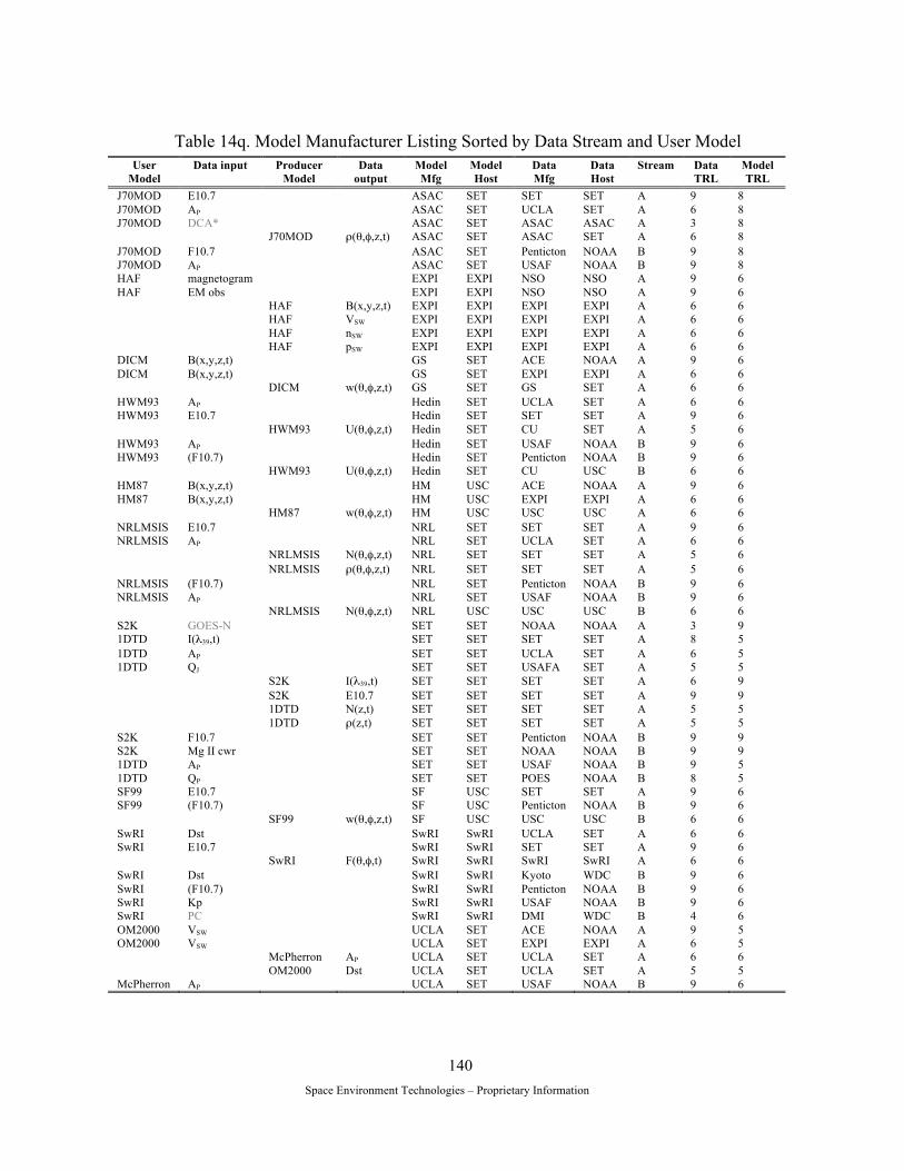
Space Environment Technologies – Proprietary Information
140
Table 14q. Model Manufacturer Listing Sorted by Data Stream and User Model
User Model
Data input Producer Model
Data output
Model Mfg
Model Host
Data Mfg
Data Host
Stream Data TRL
Model TRL
J70MOD E10.7 ASAC SET SET SET A 9 8 J70MOD AP ASAC SET UCLA SET A 6 8 J70MOD DCA* ASAC SET ASAC ASAC A 3 8 J70MOD ρ(θ,φ,z,t) ASAC SET ASAC SET A 6 8 J70MOD F10.7 ASAC SET Penticton NOAA B 9 8 J70MOD AP ASAC SET USAF NOAA B 9 8 HAF magnetogram EXPI EXPI NSO NSO A 9 6 HAF EM obs EXPI EXPI NSO NSO A 9 6 HAF B(x,y,z,t) EXPI EXPI EXPI EXPI A 6 6 HAF VSW EXPI EXPI EXPI EXPI A 6 6 HAF nSW EXPI EXPI EXPI EXPI A 6 6 HAF pSW EXPI EXPI EXPI EXPI A 6 6 DICM B(x,y,z,t) GS SET ACE NOAA A 9 6 DICM B(x,y,z,t) GS SET EXPI EXPI A 6 6 DICM w(θ,φ,z,t) GS SET GS SET A 6 6 HWM93 AP Hedin SET UCLA SET A 6 6 HWM93 E10.7 Hedin SET SET SET A 9 6 HWM93 U(θ,φ,z,t) Hedin SET CU SET A 5 6 HWM93 AP Hedin SET USAF NOAA B 9 6 HWM93 (F10.7) Hedin SET Penticton NOAA B 9 6 HWM93 U(θ,φ,z,t) Hedin SET CU USC B 6 6 HM87 B(x,y,z,t) HM USC ACE NOAA A 9 6 HM87 B(x,y,z,t) HM USC EXPI EXPI A 6 6 HM87 w(θ,φ,z,t) HM USC USC USC A 6 6 NRLMSIS E10.7 NRL SET SET SET A 9 6 NRLMSIS AP NRL SET UCLA SET A 6 6 NRLMSIS N(θ,φ,z,t) NRL SET SET SET A 5 6 NRLMSIS ρ(θ,φ,z,t) NRL SET SET SET A 5 6 NRLMSIS (F10.7) NRL SET Penticton NOAA B 9 6 NRLMSIS AP NRL SET USAF NOAA B 9 6 NRLMSIS N(θ,φ,z,t) NRL USC USC USC B 6 6 S2K GOES-N SET SET NOAA NOAA A 3 9 1DTD I(λ39,t) SET SET SET SET A 8 5 1DTD AP SET SET UCLA SET A 6 5 1DTD QJ SET SET USAFA SET A 5 5 S2K I(λ39,t) SET SET SET SET A 6 9 S2K E10.7 SET SET SET SET A 9 9 1DTD N(z,t) SET SET SET SET A 5 5 1DTD ρ(z,t) SET SET SET SET A 5 5 S2K F10.7 SET SET Penticton NOAA B 9 9 S2K Mg II cwr SET SET NOAA NOAA B 9 9 1DTD AP SET SET USAF NOAA B 9 5 1DTD QP SET SET POES NOAA B 8 5 SF99 E10.7 SF USC SET SET A 9 6 SF99 (F10.7) SF USC Penticton NOAA B 9 6 SF99 w(θ,φ,z,t) SF USC USC USC B 6 6 SwRI Dst SwRI SwRI UCLA SET A 6 6 SwRI E10.7 SwRI SwRI SET SET A 9 6 SwRI F(θ,φ,t) SwRI SwRI SwRI SwRI A 6 6 SwRI Dst SwRI SwRI Kyoto WDC B 9 6 SwRI (F10.7) SwRI SwRI Penticton NOAA B 9 6 SwRI Kp SwRI SwRI USAF NOAA B 9 6 SwRI PC SwRI SwRI DMI WDC B 4 6 OM2000 VSW UCLA SET ACE NOAA A 9 5 OM2000 VSW UCLA SET EXPI EXPI A 6 5 McPherron AP UCLA SET UCLA SET A 6 6 OM2000 Dst UCLA SET UCLA SET A 5 5 McPherron AP UCLA SET USAF NOAA B 9 6

Space Environment Technologies – Proprietary Information
141
Table 14q. Model Manufacturer Listing Sorted by Data Stream and User Model (continued) User
Model Data input Producer
Model Data out-
put Model Mfg
Model Host
Data Mfg
Data Host
Stream Data TRL
Model TRL
Joule heat
Dst USAFA SET UCLA SET A 6 5
Joule heat QJ USAFA SET USAFA SET A 5 5 Joule heat
Dst USAFA SET Kyoto WDC B 9 5
Joule heat
PC USAFA SET DMI WDC B 4 5
GAIM I(λ39,t) USC JPL SET SET A 6 6 GAIM E10.7 USC JPL SET SET A 9 6 GAIM AP USC JPL UCLA SET A 6 6 GAIM N(θ,φ,z,t) USC JPL SET SET A 5 6 GAIM U(θ,φ,z,t) USC JPL CU SET A 5 6 GAIM U(θ,φ,z,t) USC JPL NWM C/NOFS A 3 6 GAIM w(θ,φ,z,t) USC JPL GS SET A 6 6 GAIM w(θ,φ,z,t) USC JPL USC USC A 6 6 GAIM w(θ,φ,z,t) USC JPL USC USC A 6 6 GAIM w(θ,φ,z,t) USC JPL VERI C/NOFS A 3 6 GAIM F(θ,φ,t) USC JPL SwRI SwRI A 6 6 GAIM SSULI UV USC JPL DMSP SSULI A 7 6 GAIM TEC(rR,rS,t) USC JPL JPL JPL A 9 6 GAIM TEC(rR,rS,t) USC JPL CORISS C/NOFS A 3 6 GAIM TEC(rR,rS,t) USC JPL USC COSMIC A 3 6 GAIM TEC(rR,rS,t) USC JPL CORS NOAA A 8 6 GAIM TEC(rR,rS,t) USC JPL USC USC A 6 6 GAIM ne(θ,φ,z,t) USC JPL USC USC A 6 6 GAIM (F10.7) USC JPL Penticton NOAA B 9 6 GAIM AP USC JPL USAF NOAA B 9 6 GAIM N(θ,φ,z,t) USC JPL USC USC B 6 6 GAIM U(θ,φ,z,t) USC JPL CU USC B 6 6 GAIM w(θ,φ,z,t) USC JPL USC USC B 6 6 GAIM Pe,Pp USC JPL NOAA NOAA B 9 6 GAIM Ti USC JPL USC USC B 6 6 GAIM Te USC JPL USC USC B 6 6 W95 B(x,y,z,t) Weimer USC ACE NOAA A 9 6 W95 B(x,y,z,t) Weimer USC EXPI EXPI A 6 6 W95 w(θ,φ,z,t) Weimer USC USC USC A 6 6 *Light gray indicates future capability.

Space Environment Technologies – Proprietary Information
142
Table 14r. Model Manufacturer Listing Sorted by Data Stream and Producer Model
User Model
Data input Producer Model
Data output
Model Mfg
Model Host
Data Mfg
Data Host
Stream Data TRL
Model TRL
J70MOD ρ(θ,φ,z,t) ASAC SET ASAC SET A 6 8 J70MOD E10.7 ASAC SET SET SET A 9 8 J70MOD AP ASAC SET UCLA SET A 6 8 J70MOD DCA* ASAC SET ASAC ASAC A 3 8 J70MOD F10.7 ASAC SET Penticton NOAA B 9 8 J70MOD AP ASAC SET USAF NOAA B 9 8 HAF B(x,y,z,t) EXPI EXPI EXPI EXPI A 6 6 HAF VSW EXPI EXPI EXPI EXPI A 6 6 HAF nSW EXPI EXPI EXPI EXPI A 6 6 HAF pSW EXPI EXPI EXPI EXPI A 6 6 HAF magnetogram EXPI EXPI NSO NSO A 9 6 HAF EM obs EXPI EXPI NSO NSO A 9 6 DICM w(θ,φ,z,t) GS SET GS SET A 6 6 DICM B(x,y,z,t) GS SET ACE NOAA A 9 6 DICM B(x,y,z,t) GS SET EXPI EXPI A 6 6 HWM93 U(θ,φ,z,t) Hedin SET CU SET A 5 6 HWM93 AP Hedin SET UCLA SET A 6 6 HWM93 E10.7 Hedin SET SET SET A 9 6 HWM93 U(θ,φ,z,t) Hedin SET CU USC B 6 6 HWM93 AP Hedin SET USAF NOAA B 9 6 HWM93 (F10.7) Hedin SET Penticton NOAA B 9 6 HM87 w(θ,φ,z,t) HM USC USC USC A 6 6 HM87 B(x,y,z,t) HM USC ACE NOAA A 9 6 HM87 B(x,y,z,t) HM USC EXPI EXPI A 6 6 NRLMSIS N(θ,φ,z,t) NRL SET SET SET A 5 6 NRLMSIS ρ(θ,φ,z,t) NRL SET SET SET A 5 6 NRLMSIS E10.7 NRL SET SET SET A 9 6 NRLMSIS AP NRL SET UCLA SET A 6 6 NRLMSIS N(θ,φ,z,t) NRL USC USC USC B 6 6 NRLMSIS (F10.7) NRL SET Penticton NOAA B 9 6 NRLMSIS AP NRL SET USAF NOAA B 9 6 S2K I(λ39,t) SET SET SET SET A 6 9 S2K E10.7 SET SET SET SET A 9 9 1DTD N(z,t) SET SET SET SET A 5 5 1DTD ρ(z,t) SET SET SET SET A 5 5 S2K GOES-N SET SET NOAA NOAA A 3 9 1DTD I(λ39,t) SET SET SET SET A 8 5 1DTD AP SET SET UCLA SET A 6 5 1DTD QJ SET SET USAFA SET A 5 5 S2K F10.7 SET SET Penticton NOAA B 9 9 S2K Mg II cwr SET SET NOAA NOAA B 9 9 1DTD AP SET SET USAF NOAA B 9 5 1DTD QP SET SET POES NOAA B 8 5 SF99 E10.7 SF USC SET SET A 9 6 SF99 w(θ,φ,z,t) SF USC USC USC B 6 6 SF99 (F10.7) SF USC Penticton NOAA B 9 6 SwRI F(θ,φ,t) SwRI SwRI SwRI SwRI A 6 6 SwRI Dst SwRI SwRI UCLA SET A 6 6 SwRI E10.7 SwRI SwRI SET SET A 9 6 SwRI Dst SwRI SwRI Kyoto WDC B 9 6 SwRI (F10.7) SwRI SwRI Penticton NOAA B 9 6 SwRI Kp SwRI SwRI USAF NOAA B 9 6 SwRI PC SwRI SwRI DMI WDC B 4 6 OM2000 Dst UCLA SET UCLA SET A 5 5 McPherron AP UCLA SET UCLA SET A 6 6 OM2000 VSW UCLA SET ACE NOAA A 9 5 OM2000 VSW UCLA SET EXPI EXPI A 6 5 McPherron AP UCLA SET USAF NOAA B 9 6
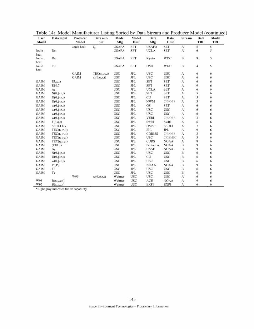
Space Environment Technologies – Proprietary Information
143
Table 14r. Model Manufacturer Listing Sorted by Data Stream and Producer Model (continued) User
Model Data input Producer
Model Data out-
put Model Mfg
Model Host
Data Mfg
Data Host
Stream Data TRL
Model TRL
Joule heat QJ USAFA SET USAFA SET A 5 5 Joule heat
Dst USAFA SET UCLA SET A 6 5
Joule heat
Dst USAFA SET Kyoto WDC B 9 5
Joule heat
PC USAFA SET DMI WDC B 4 5
GAIM TEC(rR,rS,t) USC JPL USC USC A 6 6 GAIM ne(θ,φ,z,t) USC JPL USC USC A 6 6 GAIM I(λ39,t) USC JPL SET SET A 6 6 GAIM E10.7 USC JPL SET SET A 9 6 GAIM AP USC JPL UCLA SET A 6 6 GAIM N(θ,φ,z,t) USC JPL SET SET A 5 6 GAIM U(θ,φ,z,t) USC JPL CU SET A 5 6 GAIM U(θ,φ,z,t) USC JPL NWM C/NOFS A 3 6 GAIM w(θ,φ,z,t) USC JPL GS SET A 6 6 GAIM w(θ,φ,z,t) USC JPL USC USC A 6 6 GAIM w(θ,φ,z,t) USC JPL USC USC A 6 6 GAIM w(θ,φ,z,t) USC JPL VERI C/NOFS A 3 6 GAIM F(θ,φ,t) USC JPL SwRI SwRI A 6 6 GAIM SSULI UV USC JPL DMSP SSULI A 7 6 GAIM TEC(rR,rS,t) USC JPL JPL JPL A 9 6 GAIM TEC(rR,rS,t) USC JPL CORISS C/NOFS A 3 6 GAIM TEC(rR,rS,t) USC JPL USC COSMIC A 3 6 GAIM TEC(rR,rS,t) USC JPL CORS NOAA A 8 6 GAIM (F10.7) USC JPL Penticton NOAA B 9 6 GAIM AP USC JPL USAF NOAA B 9 6 GAIM N(θ,φ,z,t) USC JPL USC USC B 6 6 GAIM U(θ,φ,z,t) USC JPL CU USC B 6 6 GAIM w(θ,φ,z,t) USC JPL USC USC B 6 6 GAIM Pe,Pp USC JPL NOAA NOAA B 9 6 GAIM Ti USC JPL USC USC B 6 6 GAIM Te USC JPL USC USC B 6 6 W95 w(θ,φ,z,t) Weimer USC USC USC A 6 6 W95 B(x,y,z,t) Weimer USC ACE NOAA A 9 6 W95 B(x,y,z,t) Weimer USC EXPI EXPI A 6 6 *Light gray indicates future capability.
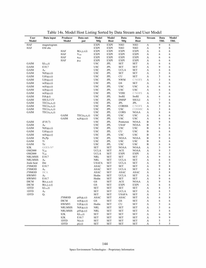
Space Environment Technologies – Proprietary Information
144
Table 14s. Model Host Listing Sorted by Data Stream and User Model
User Model
Data input Producer Model
Data out-put
Model Mfg
Model Host
Data Mfg
Data Host
Stream Data TRL
Model TRL
HAF magnetogram EXPI EXPI NSO NSO A 9 6 HAF EM obs EXPI EXPI NSO NSO A 9 6 HAF B(x,y,z,t) EXPI EXPI EXPI EXPI A 6 6 HAF VSW EXPI EXPI EXPI EXPI A 6 6 HAF nSW EXPI EXPI EXPI EXPI A 6 6 HAF pSW EXPI EXPI EXPI EXPI A 6 6 GAIM I(λ39,t) USC JPL SET SET A 6 6 GAIM E10.7 USC JPL SET SET A 9 6 GAIM AP USC JPL UCLA SET A 6 6 GAIM N(θ,φ,z,t) USC JPL SET SET A 5 6 GAIM U(θ,φ,z,t) USC JPL CU SET A 5 6 GAIM U(θ,φ,z,t) USC JPL NWM C/NOFS A 3 6 GAIM w(θ,φ,z,t) USC JPL GS SET A 6 6 GAIM w(θ,φ,z,t) USC JPL USC USC A 6 6 GAIM w(θ,φ,z,t) USC JPL USC USC A 6 6 GAIM w(θ,φ,z,t) USC JPL VERI C/NOFS A 3 6 GAIM F(θ,φ,t) USC JPL SwRI SwRI A 6 6 GAIM SSULI UV USC JPL DMSP SSULI A 7 6 GAIM TEC(rR,rS,t) USC JPL JPL JPL A 9 6 GAIM TEC(rR,rS,t) USC JPL CORISS C/NOFS A 3 6 GAIM TEC(rR,rS,t) USC JPL USC COSMIC A 3 6 GAIM TEC(rR,rS,t) USC JPL CORS NOAA A 8 6 GAIM TEC(rR,rS,t) USC JPL USC USC A 6 6 GAIM ne(θ,φ,z,t) USC JPL USC USC A 6 6 GAIM (F10.7) USC JPL Penticton NOAA B 9 6 GAIM AP USC JPL USAF NOAA B 9 6 GAIM N(θ,φ,z,t) USC JPL USC USC B 6 6 GAIM U(θ,φ,z,t) USC JPL CU USC B 6 6 GAIM w(θ,φ,z,t) USC JPL USC USC B 6 6 GAIM Pe,Pp USC JPL NOAA NOAA B 9 6 GAIM Ti USC JPL USC USC B 6 6 GAIM Te USC JPL USC USC B 6 6 S2K GOES-N* SET SET NOAA NOAA A 3 9 OM2000 VSW UCLA SET ACE NOAA A 9 5 OM2000 VSW UCLA SET EXPI EXPI A 6 5 NRLMSIS E10.7 NRL SET SET SET A 9 6 NRLMSIS AP NRL SET UCLA SET A 6 6 Joule heat Dst USAFA SET UCLA SET A 6 5 J70MOD E10.7 ASAC SET SET SET A 9 8 J70MOD AP ASAC SET UCLA SET A 6 8 J70MOD DCA ASAC SET ASAC ASAC A 3 8 HWM93 AP Hedin SET UCLA SET A 6 6 HWM93 E10.7 Hedin SET SET SET A 9 6 DICM B(x,y,z,t) GS SET ACE NOAA A 9 6 DICM B(x,y,z,t) GS SET EXPI EXPI A 6 6 1DTD I(λ39,t) SET SET SET SET A 8 5 1DTD AP SET SET UCLA SET A 6 5 1DTD QJ SET SET USAFA SET A 5 5 J70MOD ρ(θ,φ,z,t) ASAC SET ASAC SET A 6 8 DICM w(θ,φ,z,t) GS SET GS SET A 6 6 HWM93 U(θ,φ,z,t) Hedin SET CU SET A 5 6 NRLMSIS N(θ,φ,z,t) NRL SET SET SET A 5 6 NRLMSIS ρ(θ,φ,z,t) NRL SET SET SET A 5 6 S2K I(λ39,t) SET SET SET SET A 6 9 S2K E10.7 SET SET SET SET A 9 9 1DTD N(z,t) SET SET SET SET A 5 5 1DTD ρ(z,t) SET SET SET SET A 5 5

Space Environment Technologies – Proprietary Information
145
Table 14s. Model Host Listing Sorted by Data Stream and User Model (continued) User
Model Data input
Producer Model
Data output
Model Mfg
Model Host
Data Mfg
Data Host
Stream Data TRL
Model TRL
OM2000 Dst UCLA SET UCLA SET A 5 5 McPherron AP UCLA SET UCLA SET A 6 6 Joule heat QJ USAFA SET USAFA SET A 5 5 S2K F10.7 SET SET Penticton NOAA B 9 9 S2K Mg II cwr SET SET NOAA NOAA B 9 9 NRLMSIS (F10.7) NRL SET Penticton NOAA B 9 6 NRLMSIS AP NRL SET USAF NOAA B 9 6 McPherron AP UCLA SET USAF NOAA B 9 6 Joule heat Dst USAFA SET Kyoto WDC B 9 5 Joule heat PC USAFA SET DMI WDC B 4 5 J70MOD F10.7 ASAC SET Penticton NOAA B 9 8 J70MOD AP ASAC SET USAF NOAA B 9 8 HWM93 AP Hedin SET USAF NOAA B 9 6 HWM93 (F10.7) Hedin SET Penticton NOAA B 9 6 1DTD AP SET SET USAF NOAA B 9 5 1DTD QP SET SET POES NOAA B 8 5 HWM93 U(θ,φ,z,t) Hedin SET CU USC B 6 6 SwRI Dst SwRI SwRI UCLA SET A 6 6 SwRI E10.7 SwRI SwRI SET SET A 9 6 SwRI F(θ,φ,t) SwRI SwRI SwRI SwRI A 6 6 SwRI Dst SwRI SwRI Kyoto WDC B 9 6 SwRI (F10.7) SwRI SwRI Penticton NOAA B 9 6 SwRI Kp SwRI SwRI USAF NOAA B 9 6 SwRI PC SwRI SwRI DMI WDC B 4 6 W95 B(x,y,z,t) Weimer USC ACE NOAA A 9 6 W95 B(x,y,z,t) Weimer USC EXPI EXPI A 6 6 SF99 E10.7 SF USC SET SET A 9 6 HM87 B(x,y,z,t) HM USC ACE NOAA A 9 6 HM87 B(x,y,z,t) HM USC EXPI EXPI A 6 6 HM87 w(θ,φ,z,t) HM USC USC USC A 6 6 W95 w(θ,φ,z,t) Weimer USC USC USC A 6 6 SF99 (F10.7) SF USC Penticton NOAA B 9 6 NRLMSIS N(θ,φ,z,t) NRL USC USC USC B 6 6 SF99 w(θ,φ,z,t) SF USC USC USC B 6 6 *Light gray indicates future capability.

Space Environment Technologies – Proprietary Information
146
Table 14t. Model Host Listing Sorted by Data Stream and Producer Model
User Model
Data input Producer Model
Data out-put
Model Mfg
Model Host
Data Mfg
Data Host
Stream Data TRL
Model TRL
HAF B(x,y,z,t) EXPI EXPI EXPI EXPI A 6 6 HAF VSW EXPI EXPI EXPI EXPI A 6 6 HAF nSW EXPI EXPI EXPI EXPI A 6 6 HAF pSW EXPI EXPI EXPI EXPI A 6 6 HAF magnetogram EXPI EXPI NSO NSO A 9 6 HAF EM obs EXPI EXPI NSO NSO A 9 6 GAIM TEC(rR,rS,t) USC JPL USC USC A 6 6 GAIM ne(θ,φ,z,t) USC JPL USC USC A 6 6 GAIM I(λ39,t) USC JPL SET SET A 6 6 GAIM E10.7 USC JPL SET SET A 9 6 GAIM AP USC JPL UCLA SET A 6 6 GAIM N(θ,φ,z,t) USC JPL SET SET A 5 6 GAIM U(θ,φ,z,t) USC JPL CU SET A 5 6 GAIM U(θ,φ,z,t) USC JPL NWM C/NOFS A 3 6 GAIM w(θ,φ,z,t) USC JPL GS SET A 6 6 GAIM w(θ,φ,z,t) USC JPL USC USC A 6 6 GAIM w(θ,φ,z,t) USC JPL USC USC A 6 6 GAIM w(θ,φ,z,t) USC JPL VERI C/NOFS A 3 6 GAIM F(θ,φ,t) USC JPL SwRI SwRI A 6 6 GAIM SSULI UV USC JPL DMSP SSULI A 7 6 GAIM TEC(rR,rS,t) USC JPL JPL JPL A 9 6 GAIM TEC(rR,rS,t) USC JPL CORISS C/NOFS A 3 6 GAIM TEC(rR,rS,t) USC JPL USC COSMIC A 3 6 GAIM TEC(rR,rS,t) USC JPL CORS NOAA A 8 6 GAIM (F10.7) USC JPL Penticton NOAA B 9 6 GAIM AP USC JPL USAF NOAA B 9 6 GAIM N(θ,φ,z,t) USC JPL USC USC B 6 6 GAIM U(θ,φ,z,t) USC JPL CU USC B 6 6 GAIM w(θ,φ,z,t) USC JPL USC USC B 6 6 GAIM Pe,Pp USC JPL NOAA NOAA B 9 6 GAIM Ti USC JPL USC USC B 6 6 GAIM Te USC JPL USC USC B 6 6 S2K I(λ39,t) SET SET SET SET A 6 9 S2K E10.7 SET SET SET SET A 9 9 OM2000 Dst UCLA SET UCLA SET A 5 5 NRLMSIS N(θ,φ,z,t) NRL SET SET SET A 5 6 NRLMSIS ρ(θ,φ,z,t) NRL SET SET SET A 5 6 McPherron AP UCLA SET UCLA SET A 6 6 Joule heat QJ USAFA SET USAFA SET A 5 5 J70MOD ρ(θ,φ,z,t) ASAC SET ASAC SET A 6 8 HWM93 U(θ,φ,z,t) Hedin SET CU SET A 5 6 DICM w(θ,φ,z,t) GS SET GS SET A 6 6 1DTD N(z,t) SET SET SET SET A 5 5 1DTD ρ(z,t) SET SET SET SET A 5 5 J70MOD E10.7 ASAC SET SET SET A 9 8 J70MOD AP ASAC SET UCLA SET A 6 8 J70MOD DCA* ASAC SET ASAC ASAC A 3 8 DICM B(x,y,z,t) GS SET ACE NOAA A 9 6 DICM B(x,y,z,t) GS SET EXPI EXPI A 6 6 HWM93 AP Hedin SET UCLA SET A 6 6 HWM93 E10.7 Hedin SET SET SET A 9 6 NRLMSIS E10.7 NRL SET SET SET A 9 6 NRLMSIS AP NRL SET UCLA SET A 6 6 S2K GOES-N SET SET NOAA NOAA A 3 9 1DTD I(λ39,t) SET SET SET SET A 8 5 1DTD AP SET SET UCLA SET A 6 5 1DTD QJ SET SET USAFA SET A 5 5
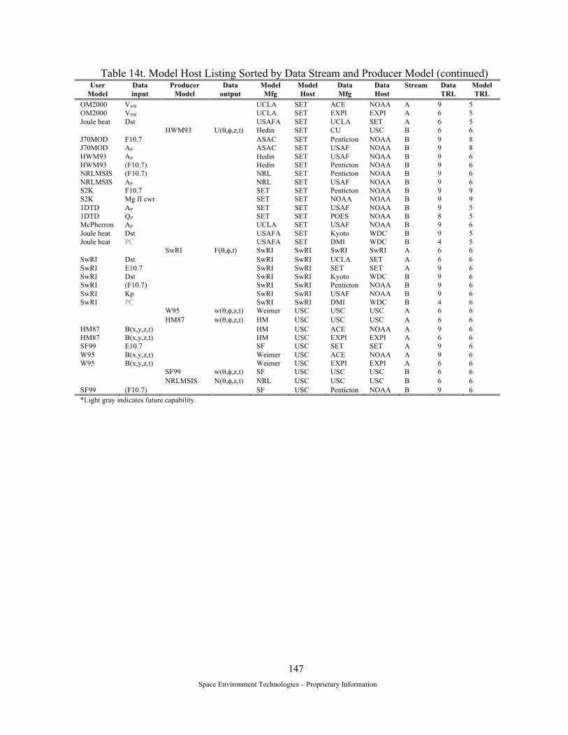
Space Environment Technologies – Proprietary Information
147
Table 14t. Model Host Listing Sorted by Data Stream and Producer Model (continued) User
Model Data input
Producer Model
Data output
Model Mfg
Model Host
Data Mfg
Data Host
Stream Data TRL
Model TRL
OM2000 VSW UCLA SET ACE NOAA A 9 5 OM2000 VSW UCLA SET EXPI EXPI A 6 5 Joule heat Dst USAFA SET UCLA SET A 6 5 HWM93 U(θ,φ,z,t) Hedin SET CU USC B 6 6 J70MOD F10.7 ASAC SET Penticton NOAA B 9 8 J70MOD AP ASAC SET USAF NOAA B 9 8 HWM93 AP Hedin SET USAF NOAA B 9 6 HWM93 (F10.7) Hedin SET Penticton NOAA B 9 6 NRLMSIS (F10.7) NRL SET Penticton NOAA B 9 6 NRLMSIS AP NRL SET USAF NOAA B 9 6 S2K F10.7 SET SET Penticton NOAA B 9 9 S2K Mg II cwr SET SET NOAA NOAA B 9 9 1DTD AP SET SET USAF NOAA B 9 5 1DTD QP SET SET POES NOAA B 8 5 McPherron AP UCLA SET USAF NOAA B 9 6 Joule heat Dst USAFA SET Kyoto WDC B 9 5 Joule heat PC USAFA SET DMI WDC B 4 5 SwRI F(θ,φ,t) SwRI SwRI SwRI SwRI A 6 6 SwRI Dst SwRI SwRI UCLA SET A 6 6 SwRI E10.7 SwRI SwRI SET SET A 9 6 SwRI Dst SwRI SwRI Kyoto WDC B 9 6 SwRI (F10.7) SwRI SwRI Penticton NOAA B 9 6 SwRI Kp SwRI SwRI USAF NOAA B 9 6 SwRI PC SwRI SwRI DMI WDC B 4 6 W95 w(θ,φ,z,t) Weimer USC USC USC A 6 6 HM87 w(θ,φ,z,t) HM USC USC USC A 6 6 HM87 B(x,y,z,t) HM USC ACE NOAA A 9 6 HM87 B(x,y,z,t) HM USC EXPI EXPI A 6 6 SF99 E10.7 SF USC SET SET A 9 6 W95 B(x,y,z,t) Weimer USC ACE NOAA A 9 6 W95 B(x,y,z,t) Weimer USC EXPI EXPI A 6 6 SF99 w(θ,φ,z,t) SF USC USC USC B 6 6 NRLMSIS N(θ,φ,z,t) NRL USC USC USC B 6 6 SF99 (F10.7) SF USC Penticton NOAA B 9 6 *Light gray indicates future capability.