c© 2019 Naman Shukla

DYNAMIC PRICING FOR AIRLINE ANCILLARIES WITH CUSTOMER CONTEXT

BY

NAMAN SHUKLA

THESIS

Submitted in partial fulfillment of the requirementsfor the degree of Master of Science in Industrial Engineering with the Advanced Analytics

Concentrationin the Graduate College of the

University of Illinois at Urbana-Champaign, 2019

Urbana, Illinois

Adviser:

Assistant Professor Lavanya Marla

ABSTRACT

Ancillaries in the travel industry have become a major source of income and profitability.

However, conventional pricing strategies are based on poorly optimized business rules that

do not respond to changing market conditions.

This study describes the dynamic pricing model that we have developed in conjunction

with Deepair solutions, an AI technology provider for travel suppliers. We present a pricing

model that provides dynamic pricing recommendations specific to each customer interaction

and optimizes expected revenue per customer. The unique nature of personalized pricing

provides the opportunity to search over the market space to find the optimal price-point of

each ancillary for each customer, without violating customer privacy.

In this study, we present and compare three approaches for dynamic pricing of ancillaries,

with increasing levels of sophistication: (1) a two-stage forecasting and optimization model

using a logistic mapping function; (2) a two-stage model that uses a deep neural network for

forecasting, coupled with a revenue maximization technique using discrete exhaustive search;

(3) a single-stage end-to-end deep neural network that recommends the optimal price. We

describe the performance of these models based on both offline and online evaluations. We

also measure the real-world business impact of these approaches by deploying them in an

A/B test on an airline’s internet booking website. We show that traditional machine learn-

ing techniques outperform human rule-based approaches in an online setting by improving

conversion by 36% and revenue per offer by 10%. We also provide results for our offline ex-

periments which show that deep learning algorithms outperform traditional machine learning

techniques for this problem.

Additionally, we propose a meta-learning approach for synchronous deployment of multiple

models. This approach is currently under production with our partner airline. Our end-to-

end deep learning model is currently being deployed by the airline in their booking system.

ii

To my parents, for their love and support.

iii

ACKNOWLEDGMENTS

I would like to express my sincere gratitude to my advisor, Dr. Lavanya Marla, for

providing continuous support during my research. I am very grateful to her for providing

me with academic guidance, crucial advice and tremendous support and encouragement. In

summary, I could not have imagined having a better advisor and mentor for my masters

studies.

I would like to acknowledge Deepair Solutions for providing a generous grant for this

project. I am profoundly grateful to Kartik Yellepeddi from Deepair Solutions, for giving

me an opportunity to work on industrial data science problems. He was always accessible

and willing to help me in my research whenever I needed, and this made my research journey

smooth and rewarding. My heartfelt thanks to Ken Otwell from Otwell Research, for invalu-

able discussion on my research project. I am very thankful to Arinbjorn Kolbeinsson from

Imperial College London, for fruitful discussions and helpful suggestion during my research.

I am extremely thankful to Dr. Bhavesh Garg, Indian Institute of Technology Ropar. His

advice and discussion helped me a lot in improving my thesis work.

I am wholeheartedly thankful to Nestor, Zhenya and Ziyu for our brainstorming sessions

and helping me finish writing my thesis. Most notably, I am thankful to Dhaya, Sathwik,

Deborshi, Kavjit, Nishant, Shashank and all others who have made the last two years so

enjoyable. I also thank my roomates Chaithanya and Vineeth for continuous support.

Finally, I am forever indebted to my parents for their unconditional love, advice, under-

standing, encouragement and sacrifices all the time.

iv

TABLE OF CONTENTS

CHAPTER 1 INTRODUCTION . . . . . . . . . . . . . . . . . . . . . . . . . . . . 11.1 Background . . . . . . . . . . . . . . . . . . . . . . . . . . . . . . . . . . . . 11.2 Related Work . . . . . . . . . . . . . . . . . . . . . . . . . . . . . . . . . . . 3

CHAPTER 2 PRICING FACTORS . . . . . . . . . . . . . . . . . . . . . . . . . . . 62.1 Demand Function . . . . . . . . . . . . . . . . . . . . . . . . . . . . . . . . . 62.2 Customer Attributes . . . . . . . . . . . . . . . . . . . . . . . . . . . . . . . 6

CHAPTER 3 PRICING MODELS . . . . . . . . . . . . . . . . . . . . . . . . . . . 113.1 Ancillary Purchase Probability Model . . . . . . . . . . . . . . . . . . . . . . 123.2 Revenue Optimization . . . . . . . . . . . . . . . . . . . . . . . . . . . . . . 133.3 Customized Loss Function for DNN-CL . . . . . . . . . . . . . . . . . . . . . 15

CHAPTER 4 PRICING MODEL EVALUATION . . . . . . . . . . . . . . . . . . . 184.1 Offline Metrics . . . . . . . . . . . . . . . . . . . . . . . . . . . . . . . . . . 184.2 Online Metrics . . . . . . . . . . . . . . . . . . . . . . . . . . . . . . . . . . 194.3 Training . . . . . . . . . . . . . . . . . . . . . . . . . . . . . . . . . . . . . . 204.4 Experiments . . . . . . . . . . . . . . . . . . . . . . . . . . . . . . . . . . . . 20

CHAPTER 5 META-LEARNING . . . . . . . . . . . . . . . . . . . . . . . . . . . . 265.1 Multi-Armed Bandit Approach . . . . . . . . . . . . . . . . . . . . . . . . . 265.2 Thompson Sampling for the Bernoulli Bandit . . . . . . . . . . . . . . . . . 285.3 Constraints, Context and Caution . . . . . . . . . . . . . . . . . . . . . . . . 305.4 Non-stationary systems and Concurrence . . . . . . . . . . . . . . . . . . . . 305.5 Online implementation for ancillary pricing at Deepair . . . . . . . . . . . . 31

CHAPTER 6 SUMMARY AND FUTURE WORK . . . . . . . . . . . . . . . . . . 326.1 Discussion . . . . . . . . . . . . . . . . . . . . . . . . . . . . . . . . . . . . . 326.2 Challenges . . . . . . . . . . . . . . . . . . . . . . . . . . . . . . . . . . . . . 326.3 Conclusion . . . . . . . . . . . . . . . . . . . . . . . . . . . . . . . . . . . . . 33

REFERENCES . . . . . . . . . . . . . . . . . . . . . . . . . . . . . . . . . . . . . . . 35

v

CHAPTER 1: INTRODUCTION

1.1 BACKGROUND

Ancillaries are optional products or services sold by businesses to complement their pri-

mary product [1]. In the airline industry, these services or products can be directly related

to a passenger’s flight itinerary, such as baggage allowance, leg room, seat upgrades or meals,

or may be related to the passenger’s overall travel plan, for example, hotel rooms, rental

cars, or destination activities. The estimated ancillary revenue collected by major US air

carriers was more than $18 billion in 2015, and $59 billion for airlines around the world in

the same year [2].

Even though this revenue stream is clearly substantial to the airline industry, its pricing

strategies are not fully developed due to its recent emergence in the market. Because these

products were traditionally not offered as ancillaries, airlines have little knowledge of the

relationship between the customers’ choice of primary product and the ancillary product.

Moreover, given the now optional nature of these products, ancillary purchases are a result

of deep personal preferences of each individual and the context of their trip. Consequently,

airlines experience very low conversion rates (less than 5%) for ancillaries. Understanding

these personal preferences based on the context of each shopping session is crucial to pricing

them effectively and generating revenue. Moreover, various ancillaries compete with each

other’s ”shelf-space” on the website and wallet-share of the customer, so pricing an ancillary

in the context of other ancillaries confounds the problem.

Currently, the majority of ancillary products are static price-points, i.e., invariant to

customer or itinerary characteristics. Our aim is to develop a price recommendation system

specific to ancillary services, to price these products dynamically based on itinerary-specific

information.

Each booking session on an airline’s website can be modeled using the state space repre-

sented in Figure 1.1. The first three steps involve the primary product, which is a set of seats

on aircraft connecting the origin to the destination, referred to as right-to-fly ; while ancillary

offerings and corresponding customer choice occur from state 4 onwards. Note that in this

work we consider only ancillaries offered during the booking session, and not those booked

later, such as adding bags after reaching the airport. The goal of this work is to optimize

prices dynamically, while estimating willingness to pay; and therefore we will address the

latter case in future work.

Conventional pricing frameworks are static, and not capable of recommending a price

1

1. User initiates a search

2. Supplier offers flight options

3. User selects a flight offer

4. Supplier offers ancillaries

5. User accepts optional ancillary offers

6. User pays and completes transaction

Figure 1.1: User live session as state space

conditioned upon rich session-specific information. Our pricing suggestions are generated

through an A/B testing framework that directs live booking traffic to various deployed

models. The integration specifications for inference and data retrieval for training, with

respect to the current pipeline at an airline booking engine, are described in Figure 1.2.

Our contributions are as follows.

• We present a rich, customized, session-specific dynamic price recommendation system

for ancillary services that significantly outperforms existing pricing systems in terms

of revenue.

• We develop a deep learning model that effectively estimates purchase probability and

simultaneously prices the ancillary product, by modeling monotonicity properties of

customers’ willingness to pay. This model provides improved revenues and captures

customers’ behavior more accurately than sequential models that combine traditional

machine learning (or deep learning) models followed by revenue optimization.

• Our model predicts human choice more accurately than our baseline model, resulting

in increased conversion for the ancillary product.

• We implement and test our models on real data, both on historical data and by live

2

testing in an airline’s booking system, and demonstrate both offline and online im-

provement based on live customer usage statistics.

Ancillary Pricing Model

Human-Curated Pricing System

Model Parameters

Internet Booking Engine (airline.com)

Scheduled Online Training

Customer Shopping and Transaction Database

Price Request & Response with

Customer Context

Price Request & Response

deepair modulesExisting interfaceAirline booking platform

A/B Testing Mode

Figure 1.2: System integration with existing pipeline

1.2 RELATED WORK

Unbundling is the process of separating a product into primary and ancillary products to

allow customers more flexibility of purchase, and businesses to increase revenues by matching

customer needs more accurately. In the airline industry, this phenomenon has been led by

low-cost carriers (LCCs), whose operational and pricing models rely heavily on ancillary

fees. In recent years, many legacy airlines have adopted this strategy [3]. Despite an initial

response through negative emotions and retaliatory behavior [4], unbundling of services

into the basic right-to-fly and additionally priced ancillary services (bags, meals, etc.) has

gradually gained acceptance among customers [5]. In fact, revenue from ancillary services in

3

the airline industry have nearly tripled in the past decade, from 3% to 8% of total revenue

[6].

Studies on this new phenomena in the airline context are ongoing [7, 8]. Economics lit-

erature indicates that the practice of offering add-ons (an equivalent term for ancillaries)

can raise equilibrium profits when airlines compete; and can also be used for price discrim-

ination and customer segmentation [9]. Allon et al[8] argue that unbundling and baggage

fees are consistent with reduction of airline operating costs, but may not effectively segment

customers. Customer characteristics and the airline’s ability to price discriminate are also

shown to significantly influence its profits [7]. Bockelie and Belobaba [1] study behavioral

models of ancillary product purchase, and specifically comparing the difference in price per-

ceptions of customers who purchase ancillary services sequentially or simultaneously. While

multiple behavioral theoretical models [10, 11, 12] based on risk perception, knowledge lev-

els and bounded rationality; and discrete choice models [13] are typically used to model

customer choice, there is limited literature that explicitly models the relationship between

ancillary services and the primary product (itinerary, or fare class).

Carrier et al [14] discussed passenger choice models extensively and extended booking-

based passenger choice models to the joint choice of an airline itinerary and fare product.

Also, additional studies provide analytical insights on the dependence of pricing models on

factors involving flow of the LCC’s like infrastructural, institutional and geographic factors

[15]. This suggests a far deeper dependence of offered service’s price on factors involving

customers and airline. Additionally, it has been studied that strategic implementation of

ancillaries in a market of heterogeneous customers requires a fine understanding of price

sensitivity. Customers sensitivity and specificity in service policies help providers to deliver

services at lower prices to majority of the costumers while sustaining the revenue margins

[16, 17]. Hence, the opportunity to model customer’s behaviour lies in correctly estimating

market’s sensitivity and demand based on customers context which inherently depends on

the factors mentioned above.

Deep neural networks have shown tremendous success on context based modeling in the

field of computer vision [18, 19, 20], natural language processing [21, 22], reinforcement learn-

ing [23, 24, 25] and others [26] as well. Also, Hornik et al [27] prominently established that

the multilayer feed forward network are the universal approximators. In addition to that,

deep neural networks have been successful in modeling highly non-linear systems including

fuzzy models [28]. Hence, this approach is an effective way of capturing extremely non-linear

dependencies in customers’ context to map market’s demand and sensitivity. Uber [29], Lyft

[30] and Airbnb [31] have effective dynamic pricing based on customers context using recent

machine learning advancements. Moreover, many other industries like electricity markets

4

[32], stock markets [33] and energy markets [34] that were traditionally using static ana-

lytic based approaches to price their products are now dynamically pricing based on recent

machine learning and deep learning models.

Topics in dynamic pricing of homogeneous products have been extensively studied [35].

In fact, dynamic pricing has been a catalyst for innovation in various transport and service

industries. Ride-hailing platforms have used surge pricing to match demand and supply,

and to avoid the “wild-goose chase” problem [29]. Related to our problem is the work

of P. Yu and J. Qian [31] for Airbnb accommodation pricing. They formulate a custom

scheme to optimally price each product using a triple-stage model with booking probability

classification, price-suggestion regression and seller-specific logic. Whereas Airbnb considers

all their listings as unique and all the customers identical, we consider the inverse problem

of identical products and unique customers.

5

CHAPTER 2: PRICING FACTORS

To correctly estimate the demand of the customers based on their specific context, analysis

of the factor of dependence is necessary. The static prices for such ancillaries are traditionally

decided based on some of these factors of dependence. Analysts use the pricing factors to

decide the suitable price for the offered ancillary. Hence, it is crucial to investigate the

pricing factors to price the ancillary correctly. In this chapter, we discuss the two primary

factors we use to determine the optimal price for an ancillary: the demand function and

customer attributes.

2.1 DEMAND FUNCTION

An estimation of a demand curve D(P ) as a function of price P , can be obtained by

evaluating the variation of demand with respect to price. Then, the optimal price can

be obtained via maximizing the expected revenue based on the estimated demand curve.

The optimal value can only be obtained when the demand function D(P ) is an accurate

estimate of the actual demand in the market, else the P ∗ and corresponding revenue will be

sub-optimal.

P ∗ = argmaxP

P ×D(P ) (2.1)

For airline ancillaries, the demand function D is not just a function of price P offered but

also of customer attributes x. Hence, a better estimation of the demand function is D(P,x)

and can be obtained by observing the change in demand conditioned on both price P and

customer attributes x. In our study, we implement and compare two algorithms to estimate

the probability of a customer purchasing an offered ancillary, which we assume to be a proxy

for estimated demand D(P,x). Details of our algorithms are presented in Chapter 3.

2.2 CUSTOMER ATTRIBUTES

We define a customer’s attributes, x, as the set of factors that influences the probability

of that customer purchasing the offered ancillary, at a given price. The major attributes

that the demand function is found to be significantly dependent on are time, market, items

already in the cart and length of stay.

6

Figure 2.1: Market clusters’ probability of ancillary purchase

2.2.1 Time

There are two types of time-related factors that heavily influence the demand function:

(1) Days to departure: Price sensitivity captures the relationship between the price and

the propensity for purchasing the product. Usually, customers who buy their tickets far in

advance are more price sensitive than customers who buy closer to departure. (2) Departure

date and time: Like the right-to-fly, ancillary demand has strong time-of-day and seasonal

variations. Itineraries starting on certain days and times have higher ‘quality’ and hence

increased demand; due to factors such as higher convenience of time of travel, better con-

nectivity (neither too long nor too short connection time), better availability of alternative

connections, special events, and holidays. The quality of service has a strong correlation

with the type of passengers it attracts. It is well-known that low quality services tend to be

cheaper and attract more price sensitive customers.

7

Figure 2.2: t-SNE plot of historical purchase based on market

2.2.2 Markets

Airlines serve a large variety of markets. A market is a tuple comprising of the origin

and destination of the trip. Certain markets are served with a larger fraction of non-stop

itineraries, while others may be served with larger fractions of itineraries containing con-

nections. Certain markets have a heavier fraction of business trips, while others consist

primarily of leisure trips.

As shown in Figure 2.1, there are clusters of markets that have high demand for ancillary

services as compared to others. To estimate the demand using (2.1), we segment these

clusters into sub-markets. We define sub-markets as a mapping from a vector of customer

attributes x to an origin-destination cluster where estimated demand is statistically similar

for a given prior ancillary price.

Visualization of historical purchases with t-SNE produces apparent separation with about

15 discrete clusters as shown in Figure 2.2. The colours are destination airports, which do

not associate with the formed clusters. Also, note that the axis represented in Figure 2.2

are the primary principal components. This signifies the presence of latent variable which

determines the basis of cluster formation. Similarly, the t-SNE plot of instances where

the ancillary is purchased (orange) and not purchased (blue) is shown in Figure 2.3. This

indicates the presence of clusters where probability of purchase is significantly higher than

8

Figure 2.3: t-SNE plot of historical purchase based on market

others. Also, some “all-blue” (no purchase) clusters are present.

Segmenting clusters of markets based on the historical demand for ancillaries seems an

important factor in estimating the demand function defined in equation (2.1).

2.2.3 Length of Stay

For those passenger bookings that are round-trips, we define Length of stay (LOS) as the

number of days a passenger plans to stay at the destination. If the passenger does not have

a return ticket we consider LOS to be 0. Figure 2.4 shows the estimated kernel density

function for LOS for two types of bookings: when an ancillary was purchased (dashed line),

and for all bookings (solid line). These estimated graphs are irregular from normalized

LOS values of 0.0 to 0.3 (approximately), indicating higher chances of ancillary purchase

for LOS durations that are neither too short nor too long. These irregularities indicate that

passengers prefer to purchase ancillaries (such as bags), for medium length trips for which

they might require additional storage space. Hence, the apparent signature describes the

conditional importance of the LOS attribute.

9

Figure 2.4: LOS signal from KDE

10

CHAPTER 3: PRICING MODELS

In this chapter, we discuss the models used to price the ancillary given the customer

context. Our pricing model consists of two components: (i) an ancillary purchase probability

model that is structured as a binary classification problem, and (ii) a revenue optimization

model that, given the probability of purchase, recommends an optimal price that maximizes

the airline’s expected revenue.

We make the following assumptions:

• Pricing range: The recommended ancillary price is allowed to vary only within a legal

range defined by business strategy as mentioned in Section 4.4.

• Monotonicity in willingness to pay : If a customer is willing to purchase a product for

price p, they are willing to purchase the same product at a price p′ < p. Similarly,

if a customer is unwilling to purchase a product at price p, they will be unwilling to

purchase at a price p′ > p.

We implement three different pricing models, of increasing complexity, shown in Figure

3.1. These are embedded into the framework in Figure 1.2.

1. Ancillary purchase prediction with logistic mapping (APP-LM): This model

uses a Gaussian Naive Bayes with clustered features (GNBC) model for ancillary pur-

chase probability prediction and a pre-calibrated logistic price mapping function for

revenue optimization.

2. Ancillary purchase prediction with exhaustive search (APP-DES): This model

uses a Deep-Neural Network (DNN) trained using a weighted cross-entropy loss func-

tion for ancillary purchase probability estimation. For price optimization, we imple-

ment a simple discrete exhaustive search algorithm that finds the optimal price point

within the pricing range.

3. End-to-End DNN with custom loss function (DNN-CL): This DNN-based

model is trained on a customized loss function, and presented in Section 3.3. This

loss function is designed using the strategic model objective function[31] and explicitly

models the dominance properties embedded within the willingness to pay assumption.

In APP-LM and APP-DES, the ancillary purchase probability model and the revenue opti-

mization model are sequential whereas in DNN-CL, they are simultaneously solved to achieve

the recommended price.

11

Human

Rules Curated By Human

APP-LM

Ancillary Purchase Prediction

(GNBC)

APP-DES End-to-End DNN-CL

Deep Neural Network with Customised

LossLogistic Mapping

Ancillary Purchase Prediction

(DNN)

Discrete Exhaustive

Search

Figure 3.1: Schematic of Ancillary Pricing Models

3.1 ANCILLARY PURCHASE PROBABILITY MODEL

Our ancillary purchase probability model estimates the demand curve within a sub-market

for each offered ancillary, for a given price of the ancillary. This is formulated as a binary

classification problem. We aim to estimate the probability distribution function fθ(x, P ),

where x | x ⊆ x, is the feature vector and P is the offered price. We used over 30 features

that fall under the following categories:

• Temporal features : Length of stay, seasonality (time of the day, month of the year,

etc), time of departure, time of shop, time to departure.

• Market-specific features : Arrival and destination airport, arrival and destination city,

ancillary popularity for the route, etc.

• Price comparison scores : Scores based on alternative/same flights across/within the

booking class.

• Journey specific features : Group size, booking class, fare group, number of stops, etc.

As mentioned earlier, the binary classification task is highly challenging because ancillary

purchase is highly imbalanced (class ratios of 6 : 100). For APP-LM, We first experiment

with many traditional classification algorithms like Gaussian Naive Bayes (GNB), Gaussian

Naive Bayes with clustered features (GNBC), Random Forest (RF), using features chosen

based on principal component analysis for these algorithms [36].

For APP-DES, we use a customized deep neural network (DNN) trained on weighted cross

entropy loss, as a classifier. While the DNN did not require a lot of feature engineering,

we experimented with various hyper-parameters like network architecture, drop-out rates,

activation functions, optimization algorithms, and convergence criteria.

12

3.2 REVENUE OPTIMIZATION

Revenue optimization is standard technique used by analysts to decide the price of a

product based on historical data. Here the idea is to maximize the expected revenue based

on demand function which is conditioned upon offered price.

3.2.1 Logistic Price Mapping Function

In our base model APP-LM, once the ancillary purchase probability is predicted, we use a

logistic function to recommend a price. The intuition behind using logistic mapping is that

the ancillary can be priced closer to the maximum of the pricing range when the probability

of purchase is high, and lower for low probabilities. Hence, a price mapping is chosen based

on (3.1).

P rec =L

1 + exp −k(x− x0)(3.1)

Pric

e of

Anc

illar

y

Probability of purchase

Aggressive pricing

Conservative pricing

Figure 3.2: Logistic mapping from probability of purchase to a recommended price.

According to (3.1), three parameters can be controlled to map the price desirably.

• Max value, L : this is the full price of the ancillary

• Shape factor, k : the shape or steepness of the curve

• Mid point, x0 : the mid point of the sigmoid curve

13

The shape factor k and mid-point x0 can be fine-tuned to be either aggressive or conser-

vative with pricing. This tuning is illustrated in Figure 3.2, indicating that at low purchase

probabilities, the model compensates by reducing the recommended price.

Algorithm 1 APP-LM Inference

1: for t = 1, 2, . . . do2: xt ← Preprocessing(x)3: P = P standard

4: Predict the probabilityp← fθ(xt, P )

5: Recommend the priceP rec = L

1+exp −k(p−x0)

6: Observe and record ground truthyt ← Offer(P rec)

7: end for

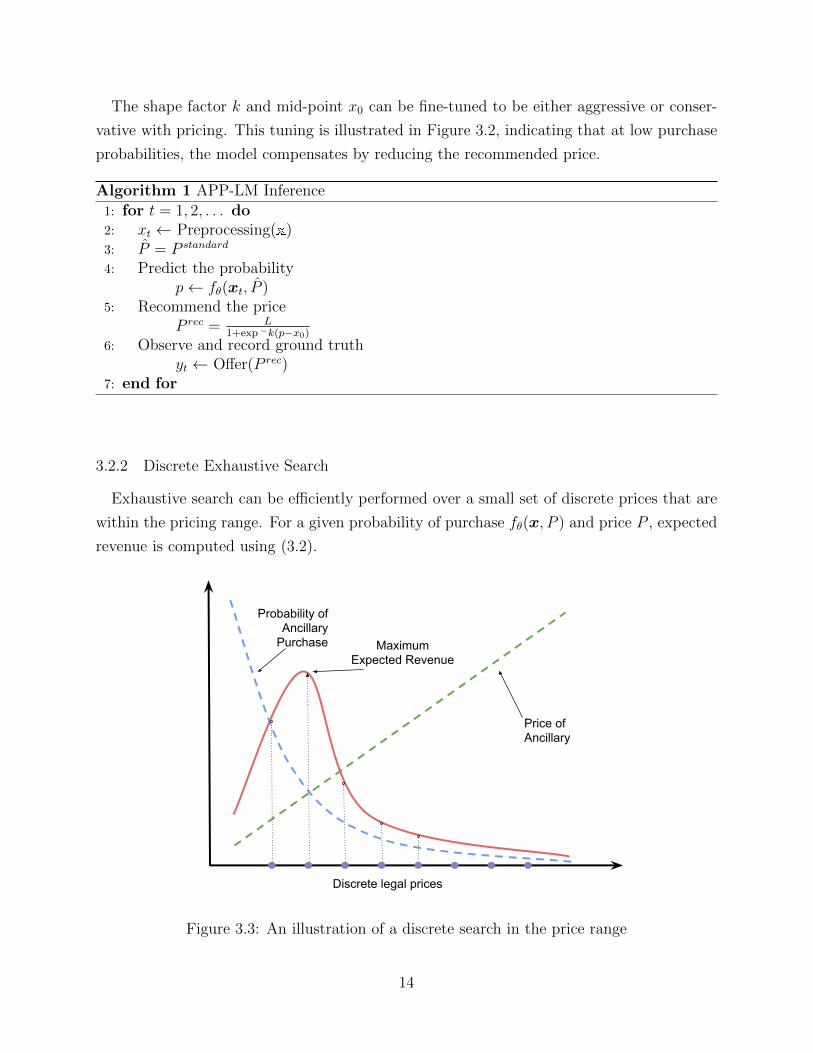
3.2.2 Discrete Exhaustive Search

Exhaustive search can be efficiently performed over a small set of discrete prices that are

within the pricing range. For a given probability of purchase fθ(x, P ) and price P , expected

revenue is computed using (3.2).

MaximumExpected Revenue

Discrete legal prices

Probability of Ancillary

Purchase

Price of Ancillary

Figure 3.3: An illustration of a discrete search in the price range

14

EP = P × fθ(x, P ) (3.2)

Without assuming that the revenue function is convex but only unimodal, an exhaustive

search over all allowed prices can be performed, as represented in Figure 3.3. The convexity

assumption is met only when price sensitivity has a small derivative in the region of interest.

Thereby, using exhaustive search, the optimal price can be evaluated using equation 3.3. As

discussed in Section 2.1, the optimality of the price P rec is dependent on the accuracy of

estimation of the demand.

P rec = argmaxP

EP (3.3)

Algorithm 2 APP-DES Inference

1: for t = 1, 2, . . . do2: xt ← Preprocessing(x)3: for P = P1, . . . ,P do4: Predict the probability of purchase

p← fθ(x, P )

5: Calculate Expected valueEP = P × p

6: end for7: Recommend ancillary price

P rec = argmaxP EP

8: Observe and record ground truthyt ← Offer(P rec)

9: end for

The performance of a two-stage sequential forecasting and optimization method (like APP-

LM and APP-DES), depends on a good demand estimate over the permissible range of

prices. This requires sufficient exposure of those prices in the market to learn an accurate

price sensitivity curve for each sub-market. Without such data, approximate methods such

as custom loss functions can produce more revenue in practice.

3.3 CUSTOMIZED LOSS FUNCTION FOR DNN-CL

In this section, we present a customized loss function that takes into account a regret of

pricing low, conditional on the ancillary being purchased; and a penalty for recommending

15

high, conditional on it not being purchased. The objective function is inspired from the

strategic model proposed by [31] and ε-insensitive loss used in SVR[37]. We enhance this

strategic model using latent variables to incorporate the monotonicity in the willingness to

pay assumption in our loss function. Suppose we are given N training samples {xi, yi}Ni=1,

where xi is the feature vector and yi is the ground truth label for the ith session. For

purchased ancillaries, yi equals 1 and 0 otherwise. The recommended price P rec for feature

vector x is denoted by P rec = FΘ(x,P), where Θ is a set of trainable parameters that can

be learned for the mapping function F, and P is a set of discrete price points in the pricing

range.

The objective of the learning is to minimize the loss L given as

L = argminθ

N∑i=1

|P|∑j=1

(Φlb + Φub) · 1(σij>0) (3.4)

where the lower bound function Φlb and upper bound function Φub are defined as,

Φlb = max

(0,(L(Pij, δij)− FΘ(xi,P)

))Φub = max

(0,(FΘ(xi,P)− U(Pij, δij)

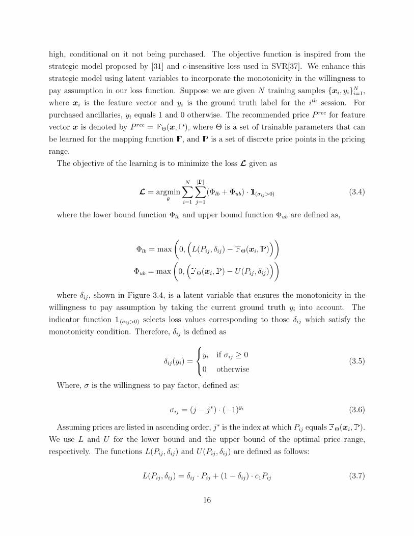
))where δij, shown in Figure 3.4, is a latent variable that ensures the monotonicity in the

willingness to pay assumption by taking the current ground truth yi into account. The

indicator function 1(σij>0) selects loss values corresponding to those δij which satisfy the

monotonicity condition. Therefore, δij is defined as

δij(yi) =

yi if σij ≥ 0

0 otherwise(3.5)

Where, σ is the willingness to pay factor, defined as:

σij = (j − j∗) · (−1)yi (3.6)

Assuming prices are listed in ascending order, j∗ is the index at which Pij equals FΘ(xi,P).

We use L and U for the lower bound and the upper bound of the optimal price range,

respectively. The functions L(Pij, δij) and U(Pij, δij) are defined as follows:

L(Pij, δij) = δij · Pij + (1− δij) · c1Pij (3.7)

16

Pi1 Pi2 Pi3 Pi4 Pi5 Pi6

Pi1 Pi2 Pi3 Pi4 Pi5 Pi6

yi = δi. = 1

Ancillary purchasedAncillary not purchased

yi = δi. = 0

yi : ground truth

δi4 : latent variableδi3δi2δi1

δi3 δi4 δi5 δi6

yi

Figure 3.4: Latent variable δ mapping from ground truth y

When the ancillary is purchased, the lower bound L is the purchase price Pij. Otherwise,

a lower price of c1Pij is set to be the lower bound, where c1 ∈ (0, 1).

U(Pij, δij) = (1− δij) · Pij + δij · c2Pij (3.8)

The upper bound U is Pij when the ancillary is not purchased, whereas if the ancillary is

purchased, a price of c2Pij (c2 > 1) is set as the upper bound.

Table 3.1: Lower bound and Upper bound loss values

Prices Φlb · 1(σij>0) Φub · 1(σij>0)

Pij < FΘ 0 max(0,FΘ(xi,P)− c2Pij)Pij = FΘ 0 0Pij > FΘ max(0, c1Pij − FΘ(xi,P)) 0

Table 3.1 illustrates the lower and upper bound loss values for recommended price with

respect to discrete price points. For Pij < FΘ(xi,P), the upper bound loss increases linearly.

For upper bound loss to be non-zero, c2 >FΘ(xi,P)

Pij. Similarly, for non-zero loss, the bounds

on c1 are set to FΘ(xi,P)Pij

< c1 < 1. For c1 = c2 = 1, the lower bound and upper bound are

equal and hence the optimal price will be the jth price in the price set P. Therefore, c1 and

c2 can be chosen to change the gap between the lower and upper bounds.

17

CHAPTER 4: PRICING MODEL EVALUATION

In the absence of optimal price values or the best hindsight strategy, it was important

to the airline to define a set of offline and online metrics. Offline metrics are useful for

model development, incremental learning, hyper-parameter optimization while online metrics

measure business value. Establishing the exact set of offline metrics that correlates with

online business metrics is an active area of research.

4.1 OFFLINE METRICS

In this section, we define the metrics that we use to serve as guides through hyper-

parameter tuning and to ensure that nightly update of DNN weights do not overfit the

data. We use the Price Decrease Recall (PDR) and Price Decrease Precision (PDP) scores

presented by [31] due to their high correlation with the airline’s business metrics. PDR

measures how likely our recommended prices are lower than the current offered prices for

non purchased ancillary and PDP measures the percentage for recommended prices that

are lower than current offered prices for non purchased ancillary. Additionally, we use the

following metrics:

4.1.1 Area Under the Curve (AUC)

Due to presence of high class imbalance as discussed in Section 3.1, we used the AUC of the

Receiver Operating Characteristic (ROC) Curve as the offline metric to compare ancillary

purchase prediction model performance.

4.1.2 Regret Score (RS)

In recent work [31], regret score has been chosen as an offline evaluation criterion because

of its proportional relationship to the business metric. RS is defined by equation (4.1).

RS = meanpurchases

(max

(0, 1− P rec

P

))(4.1)

Intuitively, RS measures on an average how close our recommended price P rec was to the

true purchase price P . For the example set of sessions in Table 4.1, sessions 1, 2 and 5 have

0.20, 0.20 and 0.75 regret respectively. Because sessions 3 and 4 have recommended price

higher than purchased, regret is 0. Therefore, RS values for this sample of sessions is 0.095.

18

Table 4.1: Example prices for purchased sessions

Session # Purchase Price Recommended Price

1 10 82 15 123 10 154 25 355 40 37

4.1.3 Price Decrease F1 (PDF1)

This score is inspired by the F1 score used to evaluate the precision and recall trade-off.

PDF1 therefore measures the trade-off between PDR and PDP according to (4.2).

PDF1 =2 · PDR · PDPPDR + PDP

(4.2)

4.2 ONLINE METRICS

Online metrics represent real-world business metrics that indicate if a model is driving

business value. We use two key metrics to measure the performance of a model in the real

world.

4.2.1 Conversion Score

One of the primary business metric is the conversion ratio, i.e., the percentage of offers

that are being purchased and converted into orders.

Conversion Score =Number of purchases

Total number of sessions(4.3)

4.2.2 Revenue per session

The revenue per session (RPS) metric is one of the most essential business metrics to

quantify actual performance.

19

4.3 TRAINING

All of our deep neural network models (in APP-DES and DNN-CL) are trained on NVIDIA

Tesla K80 GPU. We used stochastic gradient descent (SGD)[38] with a decaying learning rate

to optimize the loss function. Mini-Batches and drop-out units [39, 40] are used to regularize

model training. For a discrete exhaustive search over the prices (see Section 3.2.2), we use

a mini-batch of the allowed price inputs to enable a single call to the GPU which minimizes

data transfer and model setup cost for each price selection event. Hyperparameters like c1

and c2 are tuned using the bounds for non-zero loss and the upper-lower bound gap (see

Section 3.3) over the median price point in set P. We also use the scheduled mini-batch

training approach for online model training. Figure 4.1 shows online training loss values for

incremental training of DNN based model.

Figure 4.1: Loss curves for different online training sessions

4.4 EXPERIMENTS

During the first phase of online experimentation, our airline partner’s business strategy is

to recommend prices equal to or less than the current human-offered price. Although this

strategy reduces the search space considerably, the business motivation behind it is to reduce

the overall friction in the traveler’s journey by providing them an incentive to pre-purchase

ancillaries online. Therefore, the aim of our online experiment is to offer discounts in an

intelligent way, so that we improve the conversion rate of ancillaries without dropping the

revenue per offer. This also has a potential negative impact of increasing conversion score

without improving revenue per session. Therefore, as mentioned in Section 4, using the right

set of metrics for evaluation is crucial.

20

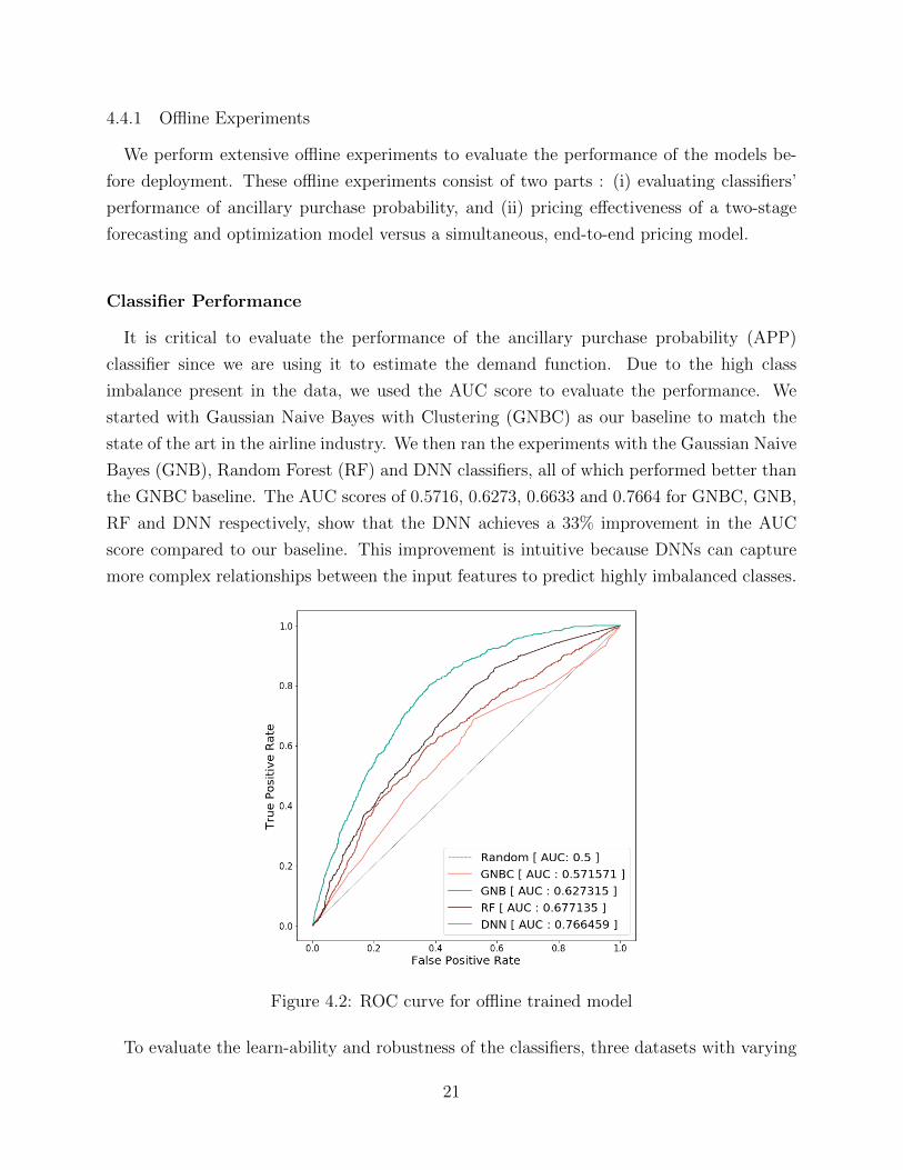
4.4.1 Offline Experiments

We perform extensive offline experiments to evaluate the performance of the models be-

fore deployment. These offline experiments consist of two parts : (i) evaluating classifiers’

performance of ancillary purchase probability, and (ii) pricing effectiveness of a two-stage

forecasting and optimization model versus a simultaneous, end-to-end pricing model.

Classifier Performance

It is critical to evaluate the performance of the ancillary purchase probability (APP)

classifier since we are using it to estimate the demand function. Due to the high class

imbalance present in the data, we used the AUC score to evaluate the performance. We

started with Gaussian Naive Bayes with Clustering (GNBC) as our baseline to match the

state of the art in the airline industry. We then ran the experiments with the Gaussian Naive

Bayes (GNB), Random Forest (RF) and DNN classifiers, all of which performed better than

the GNBC baseline. The AUC scores of 0.5716, 0.6273, 0.6633 and 0.7664 for GNBC, GNB,

RF and DNN respectively, show that the DNN achieves a 33% improvement in the AUC

score compared to our baseline. This improvement is intuitive because DNNs can capture

more complex relationships between the input features to predict highly imbalanced classes.

Figure 4.2: ROC curve for offline trained model

To evaluate the learn-ability and robustness of the classifiers, three datasets with varying

21

amount of data are used. Datasets A, B and C have 41, 000, 50, 000 and 72, 000 sessions

respectively. Results from our experiments are in Table 4.2. DNN shows most dominant

signs of learn-ability with increasing dataset size. The best performance of these classifiers

on the validation set is also presented as an ROC curve in Figure 4.2.

Table 4.2: AUC score of models on datasets.

Dataset GNBC GNB RF DNN

A 0.5444 0.6013 0.6646 0.6755B 0.5274 0.6186 0.6771 0.6967C 0.5716 0.6273 0.6633 0.7664

Pricing effectiveness of a sequential two-stage model versus a simultaneousend-to-end model

Although the DNN performs well for Ancillary Probability Prediction, it was important to

also measure the effectiveness of the final price recommendations from each pricing model.

We used the offline metrics defined in Section 4.1 to perform the comparison between the

two-stage sequential forecasting and optimization models (APP-LM and APP-DES), and

the simultaneous end-to-end pricing model (DNN-CL). Given the business requirement to

provide discounts on the human-recommended price, we considered Regret Score (RS) and

Price Decrease Recall (PDR) as more important than PDP and PDF1 [31]. Our results

are summarized in Table 4.3. The APP-LM (which uses our baseline APP model and is

manually tuned through a parameter search), serves as our baseline for pricing effectiveness.

The inefficient performance of the APP-DES model on these metrics despite the estimation of

a good APP model in the first step suggests that the price-demand relationship (see Figure

3.3) is not estimated accurately. This shortcoming is overcome by the end-to-end model

(DNN-CL), which not only overcomes the effect of this inaccuracy but also outperforms the

APP-LM on all four metrics.

Table 4.3: Comparison of scores for different models in offline experiments.

Scores APP-LM APP-DES DNN-CL

RS 0.0741 0.3776 0.0726PDR 0.6366 0.6303 0.8294PDP 0.9276 0.9320 0.9230PDF1 0.7550 0.7520 0.8737

22

Hence, we conclude that the DNN-CL model not only minimizes the regret for not pricing

high for purchased ancillaries, but also maximizes the likelihood of the recommended prices

being low when ancillaries are not purchased.

4.4.2 Online Experiments

Our APP-LM model has been deployed in production on our partner airline’s internet

booking engine for model validation. The APP-DES and the DNN-CL models are currently

under deployment, following their successful performance according to the offline metrics.

Table 4.4: Conversion percentage and revenue generated by our model (APP-LM) comparedto human-curated and random prices

Pricing System Avg. Revenue per Offer Conversion Score

HUMAN 1.00 10.18%RANDOM 0.77 12.37%APP-LM 1.10 13.92%

According to the airline’s business strategy, we introduced a random discount model in

addition to the APP-LM model. This random discount model is allowed to recommend

discounted prices based on Gaussian noise. There are two reasons for deploying a random

price recommender. First, it establishes a baseline for conversion score improvements from

discounted ancillaries. Second, it enables us to explore various prices and calibrate price

sensitivity. The deployed models are compared with both human-curated static prices and

prices from the random discount model. All three were deployed concurrently in an A/B

testing setting for a period of 120 days. The results of this comparison for the most recent

30 days are shown in Table 4.4.

Figure 4.4 and Table 4.4 indicate that the random discount model is able to produce higher

conversion rates than the human-curated pricing system. This not only demonstrates the

existence of price sensitivity among customers, but also allows us to measure it. Additionally,

the random discount model is unable to produce higher revenue per offer because it conflates

the sub-markets’ demand and makes them indistinguishable, thus losing information.

Because customers’ price sensitivity is observed through the random discount model, a

slight increase in the conversion score was expected in our deployed model APP-LM. The

results in Table 4.4, Figure 4.3 and Figure 4.41 confirm this expectation. We observe a 36%

1The exact dates and revenue figures cannot be included due to proprietary, privacy and sensitivityrestrictions

23

1 3 5 7 9 11 13 15 17 19 21 23 25 27 29

Reve

nue

Per O

ffer

Days

01. HUMAN 02. RANDOM 03. APP-LM

Figure 4.3: Revenue Per Offer by Each Pricing System Over Time

0%

5%

10%

15%

20%

25%

30%

1 3 5 7 9 11 13 15 17 19 21 23 25 27 29

Conversion

Days

01. HUMAN 02. RANDOM 03. APP-LM

Figure 4.4: Conversion Score by Each Pricing System Over Time

24

increase in conversion rate, which is a 15% increase compared to the random discount model.

More importantly, our model produces 10% more revenue than the human-curated pricing

system. This implies that our model recommends lower prices to targeted customers such

that the revenue per offer from our model can still outperform (or at least be comparable to)

the human-curated pricing system. For revenue per offer and conversion score, we see that

our model can indeed capture the market trend in a timely fashion. Furthermore, the clear

trend of both higher revenue and higher conversion score with respect to the human-curated

system indicate the accuracy of target discount with the customer’s context.

25

CHAPTER 5: META-LEARNING

As discussed in Chapter 4, the online business performance of our deployed models is,

on average, consistently better than human rule-based approaches. However, as is apparent

from Figure 5.1, no one model dominates in performance, resulting in an erratic trend in in

the revenue per offer among the models deployed online. The results in Figure 5.1 are due

to a pre-configured standard A/B testing framework in the system of a real airline, in which

the percentage share of online traffic share for each model is given by Figure 5.2. The next

question of interest, therefore, is a meta-learning approach that directs traffic efficiently to

the right model for that session.

Figure 5.1: Model online performance on business metric

We now model the traffic share value as a meta-parameter, which can then be tuned for

targeting traffic more effectively to the better performing model. Learning this parame-

ter is therefore critical to identify the “winning” model and separate it from other mod-

els. Based on customers’ responses (to purchase an ancillary or not), we can reinforce the

meta-parameters to adapt to the outcome. The multi-armed bandit approach is one such

reinforcement learning technique that accomplishes this exact task.

5.1 MULTI-ARMED BANDIT APPROACH

The multi-armed bandit problem is an extensively studied reinforcement learning tech-

nique which is widely used as a part of A/B testing [41, 42]. Solving this problem involves

26

Figure 5.2: Online traffic share and discount points

determining a sequence of decisions to choose from a given action space, with the reward

associated with each action or ‘arm’ only partially known (or having a random component).

The environment (“nature”) reveals a reward after each action is taken, thereby also reveal-

ing more information about the random component of that action’s reward. The objective

of the problem is to maximize the expected rewards, i.e., minimize the cumulative expected

regret [43]. The bandit problem involves trade off between exploitation and exploration

since the reward is only revealed for the chosen action. Hence, this problem setting makes

if perfectly suitable for A/B testing. At each possible action step, the tradeoff made by

the decision-maker is to exploit the action that has the highest expected tradeoff with the

updated information available until that point, and to explore other actions to gather more

information about the random component of the reward of those actions, to maximize gain

in the long run.

In our framework, each of the multiple models is viewed as an arm of the multi-armed ban-

dit problem. This enables the decision-maker to direct online traffic based on the customer’s

response to the price offered by that arm. Hence, this meta-learning approach provides

a trainable mechanism to allocate customer traffic to the arms during the test based on

performance. Furthermore, meta-learning allows potentially different expected conversion

rates of the different arms in an online setting. We explore one of the techniques to solve the

multi-arm bandit problem, called Thompson Sampling , to allow us to exploit arms that have

performed well in the past and explore seemingly inferior arms in case it might outperform

the current winning arm [44, 45].

27

5.2 THOMPSON SAMPLING FOR THE BERNOULLI BANDIT

In a Bernoulli bandit problem, there are a total of A valid actions. An action at ⊆ A at

time t produces a reward rt ∈ {0, 1} of one with probability θa and zero with probability

1 − θa. The mean reward θ = (θ1, . . . , θA) is assumed to be unknown, but is constant over

time. The agent begins with an independent prior belief over each θk. As observations

are gathered, the distribution is updated according to Bayes rule. The priors, according to

equation 5.1, are assumed to be beta-distributed with parameters αa ∈ {α1, . . . , αA} and

βa ∈ {β1, . . . , βA}. In particular, the exact prior probability density function given for an

action a is,

pbeta(θa) =Γ(αa + βa)

Γ(αa)Γ(βa)θ(αa−1)a (1− θa)(βa−1) (5.1)

where Γ denotes the gamma function. The beta distribution is particularly suited to this

computation because it is a conjugate prior to the Bernoulli distribution [45].

5.2.1 Simulation

In this section we discuss an offline simulation performed on synthetic data to show the

convergence rate of Thompson Sampling. Here, we have initialized three experimental models

that have a success rate of 0.45, 0.55 and 0.60. The aim of this simulation is to achieve this

success rate through multi-armed bandit approach. The algorithm 3 presents the pseudocode

of the implementation used for simulation.

Algorithm 3 Thompson Sampling for the Bernoulli Bandit

1: for t = 1, 2, . . . do2: for a = 1, . . . , A do3: Sample θa ∼ Beta(αa, βa)4: end for5: xt ← argmaxa θa6: Apply xt7: Observe rt8: (αxt , βxt)← (αxt + rt, βxt + 1− rt)9: end for

We start the simulation with the prior θ0 = Beta(α = 1, β = 1), which corresponds

to a uniform prior between 0 and 1. Note the initial uniform distribution can be seen in

Figure 5.3. The run is then simulated for 2000 steps and target probabilities are recorded.

In practice, the simulation results converged in approximately 1000 steps. Table 5.1 shows

28

the convergence of the Thompson Sampling approach for the multi-armed bandit problem,

demonstrating that the latent probability distribution can be inferred using this approach.

Table 5.1: Simulation results for Thompson Sampling

θ True probability Simulated probability Trials

θ1 0.45 0.45 70θ2 0.55 0.55 305θ3 0.60 0.61 1625

The visualization of the convergence in the beta distribution with respect to the itera-

tions is shown in Figure 5.3. We thus conclude that convergence in finding the best arm

can be achieved in a controlled environment where the latent probability distribution is

temporally invariant, i.e., it belongs to a stationary system. For problems involving tempo-

ral dependence, convergence can only be estimated in an online setting, i.e., instantaneous

environment and agent response [46].

Figure 5.3: Convergence of the Distribution using Thompson Sampling

29

5.3 CONSTRAINTS, CONTEXT AND CAUTION

Thompson sampling can be applied fruitfully to a broad array of online decision problems

beyond the Bernoulli bandit. Thompson sampling outperforms other stochastic bandit algo-

rithms (KL-UCB, Bayes UCB, UCB, ε-greedy etc) on most bandit-type problems [44]. But

in problems involving time-varying constraints on the action, line 5 in Algorithm 3 has to

modified.

Another extension of the multi-armed bandit approach addresses contextual online deci-

sion problems. In these problems, the choice of the arm in a multi-armed bandit at also

depends on an independent random variable zt that the agent observes prior to making the

decision. In such scenarios, the conditional distribution of the response yt is of the form

pθ(·|at, zt). Contextual bandit problems of this kind can be addressed through augmenting

the action space and introducing time-varying constraint sets by viewing action and con-

straint together as at = (at, zt), with each arm (choice) represented as At = {(at, zt : a ∈ A)},where A is the set from which xt must be chosen. After which it is straightforward to apply

thompson sampling to select action.

In certain situations when models have a particular baseline criteria to maintain, caution-

based sampling can be used [45]. This can be accomplished through constraining actions

for each time tth step to have lower bound on expected average reward as At = {a ∈ A :

E[rt|at = a] ≥ r}. This ensures that expected average reward at least exceeds r using such

actions.

5.4 NON-STATIONARY SYSTEMS AND CONCURRENCE

So far, we discussed settings in which model parameters θ are constant over time i.e.

belong to a stationary system. In practice, the decision-maker could face a non-stationary

system, which is more appropriately modeled by time-varying parameters, such that reward

is generated by pθt(·|at). In such contexts, the arm of the problem will never stop exploring,

which could be a potential drawback. A more robust method involves ignoring all historical

observations made prior to a certain time period τ in the past [47]. Now, decision-makers

produce a posterior distribution after every time step t based on the prior and conditioned

only on the most recent τ actions and observations. Model parameters are sampled from

this distribution, and an action is selected to optimize the associated model.

Dynamic pricing is one such problem where a single recommendation could be a weighted

sum of recommendations from multiple arms, a concept referred to as concurrence [48]. This

is a case where the decision-maker takes multiple actions (arms) concurrently. Concurrency

30

can be predefined with number of fixed arms to be pulled every time or it could be coupled

with baseline caution (discussed in Section 5.3). This approach is similar to an approach

based on an ensemble of models.

5.5 ONLINE IMPLEMENTATION FOR ANCILLARY PRICING AT DEEPAIR

Although the assumption of models being temporally stable is a crucial assumption while

using Thompson Sampling in multi-armed bandit settings, the offline simulations we per-

formed for meta-learning provide reasonable evidence of convergence to the true distribution

[49, 50] of the choice of models. Hence, our meta-learning approach shows promising offline

results on synthetic data. For online deployment in the airline’s systems, meta-learning using

a multi-armed bandit approach can be used to route incoming customer bookings to each

of the considered models, which serve as arms of the bandit. Additionally, meta-learning

could also potentially handle concurrency by pricing using multiple models. Currently, meta-

learning based models are being deployed to our partner airlines without concurrency being

enabled, with the concurrency feature under development. Using targeted traffic routing, we

hope to further improve our online metrics of evaluation as far as business value is considered.

We are actively developing models that can improve the estimation accuracy.

31

CHAPTER 6: SUMMARY AND FUTURE WORK

6.1 DISCUSSION

Historically, price sensitivity to ancillaries has not been captured due to static pricing.

However, it is critical to capture customers’ price sensitivity to price ancillaries correctly

to match customer needs and maximize airline revenues. Currently, all of the models we

proposed in Chapter 4 - APP-LM, APP-DES and DNN-CL - show promise, and are contin-

ually being tuned further to capture and train on the ground truth responses of customers.

While APP-LM has been deployed online, APP-DES and DNN-CL are in the process of

being deployed. Once model validation is performed online, the airline’s booking system will

switch to the most robust model. For the APP-DES and DNN-CL models, we are specifi-

cally interested in further examining the correlation between offline model performance to

online business performance, because they outperform APP-LM in offline experimentation.

Further, our deployment system will be transitioned from a scheduled mini-batch training

(see Section 4.3), to an event-wise online training. This transition will enable the model to

accurately learn temporal dependencies. We also plan to alter the current business strategy

(see Section 4.4) to allow our model to recommend prices higher then current limit, and

observe customer responses. Finally, we plan to study the effect of heterogeneous ancillary

types being dynamically priced by our deployed models, and the best predicted subset of

ancillaries being offered to the customer. Given that various ancillaries compete for wallet-

share and shelf-space, it will help expand our understanding of whether such pricing models

compete, or collaborate, with each other.

6.2 CHALLENGES

In our study, we have shown that the estimation of the demand curve is possible by esti-

mating the probability of purchase. The foundations of our pricing models like APP-LM and

APP-DES are based on this (see Section 3.1) idea. Sequential estimation of demand curve

including price optimization with high efficiency is a challenging task. This is due to the

presence of variability in the estimation step, followed by sub-optimal solution of the price

optimization problem. Challenges arise because the components of such sequential mod-

els can be highly interdependent and thereby susceptible to the co-variability. Practically,

techniques like market wise clustering, ensembling of models and meta learning seems to be

effective in mitigating the effects of high interdependence [51]. This is one of the reasons why

32

our cluster based models (GNBC) and ensemble of models (DNN) [39] are able to perform

significantly better.

Also, we proposed our custom loss model as a better alternative to the current method

of optimal pricing (see Section 3.3). We have also successfully demonstrated the significant

improvement on overall performance of DNN-CL over APP based models as well as human

rule-based approaches. However, a caveat corresponding to improved hyperparameter tuning

needs to be addressed. Parameters that describe the lower and upper bounds of the loss

function have to be tuned correctly in order to achieve superior performance of the DNN-

CL model. Hence, the challenge is to find the optimal values for such hyperparameters

without having any intuition behind the architecture. Additionally, hyperparameter search

on two drastically different settings, namely online and offline, increases the complexity of

the problem tremendously.

Finally, our meta-learning framework which aims to direct the traffic to specific models in

an online setting is yet to be tested on real environment. Even though the offline simulation

results in a controlled setting are promising, the customers ground truth response are yet to

be measured. The temporal dependence on traffic routing probability can only be observed

when meta-learning is performed live with customers making choices based on the models’

recommendations. Therefore, estimating the rate of convergence is another crucial challenge.

Moreover, non-convergence of the probability distribution might lead to over-exploration.

This challenge can only be addressed once the meta-learning receives feedback from the

online environment.

6.3 CONCLUSION

In this work, we presented a first step in the direction of efficient customized pricing sys-

tems based on machine learning for ancillary prices from booking data in the airline industry,

compared to past works that focus on strategic impacts. We successfully demonstrate that

ancillaries can be dynamically priced without using any user specific information that vi-

olates customer privacy. We compared three different dynamic pricing models (APP-LM,

APP-DES and DNN-CL) and their associated frameworks. Our results show that the accu-

racy of estimating the demand and fine-tuning its sensitivity to price, greatly influences the

optimality of the recommended price. Our offline experiments indicate that DNN-CL can

perform significantly better than APP-LM, APP-DES, and currently deployed approaches, to

maximize revenue. In online experiments, our APP-LM model outperforms human-curated

pricing systems currently in use. By using reliable evaluation metrics that correlate well

with business impact, we hope to observe further improvement in online metrics through

33

our APP-DES and DNN-CL models that are currently under deployment. Furthermore,

our work on meta-learning shows ancillary price recommendations from multiple concurrent

models in a competitive setting. Our work demonstrates the promise of improved busi-

ness value through highly accurately, continuously updated models for customer demand for

ancillaries, and their sensitivity to prices.

34

REFERENCES

[1] A. Bockelie and P. Belobaba, “Incorporating ancillary services in airline passenger choicemodels,” Journal of Revenue and Pricing Management, vol. 16, no. 6, pp. 553–568, 2017.

[2] IdeaWorks, “Airline ancillary revenue projected to be 59.2 billion dollar world-wide in 2015,” https://www.ideaworkscompany.com/wp-content/uploads/2015/11/Press-Release-103-Global-Estimate.pdf, 2015, ideaWorks Article.

[3] L. Garrow, S. Hotle, and S. Mumbower, “Assessment of product debundling trends inthe us airline industry: customer service and public policy implications,” TransportationResearch Part A, vol. 46, pp. 255–268, 2012.

[4] S. Tuzovic, M. C. Simpson, V. G. Kuppelwieser, and J. Finsterwalder, “From free to fee:Acceptability of airline ancillary fees and the effects on customer behavior,” Journal ofRetailing and Consumer Services, vol. 21, no. 2, pp. 98–107, 2014.

[5] J. F. O’Connell and D. Warnock-Smith, “An investigation into traveler preferences andacceptance levels of airline ancillary revenues,” Journal of Air Transport Management,vol. 33, pp. 12–21, 2013.

[6] T. Stalnaker, K. Usman, and A. Taylor, “Airline economic analysis,”https://www.oliverwyman.com/content/dam/oliver-wyman/global/en/2016/jan/oliver-wyman-airline-economic-analysis-2015-2016.pdf, 2016.

[7] Y. Cui, I. Duenyas, and O. Sahin, “Unbundling of ancillary service: How does pricediscrimination of main service matter?” Working Paper, 2016.

[8] G. Allon, A. Bassamboo, and M. Lariviere, “Would the social planner let bags fly free?”Working Paper, 2011.

[9] G. Ellison, “A model of add-on pricing,” Quarterly Journal of Economics, vol. 120, pp.585–637, 2005.

[10] D. Kahneman and A. Tversky, “Prospect theory: an analysis of decision under risk,”Econometrica, vol. 47, pp. 263–292, 1979.

[11] X. Gabaix and D. Laibson, “Shrouded attributes, consumer myopia, and informationsuppression in competitive markets,” Quarterly Journal of Economics, vol. 121, pp.505–540, 2006.

[12] J. Shulman and X. Geng, Management Science, vol. 59, pp. 899–917, 2013.

[13] M. Ben-Akiva and S. Lerman, Discrete choice analysis. MIT Press, Cambridge, MA,1985.

[14] E. Carrier, “Modeling the choice of an airline itinerary and fare product using bookingand seat availability data,” Ph.D. dissertation, Massachusetts Institute of Technology,Department of Civil and Environmental , 2008.

35

[15] M. Ishutkina and R. J. Hansman, “Analysis of interaction between air transportationand economic activity.” in The 26th Congress of ICAS and 8th AIAA ATIO, 2008, p.8888.

[16] X. Geng and J. D. Shulman, “How costs and heterogeneous consumer price sensitivityinteract with add-on pricing,” Production and Operations Management, vol. 24, no. 12,pp. 1870–1882, 2015.

[17] F. Ancarani, E. Gerstner, T. Posselt, and D. Radic, “Could higher fees lead to lowerprices?” Journal of Product & Brand Management, vol. 18, no. 4, pp. 297–305, 2009.

[18] J. Gu, Z. Wang, J. Kuen, L. Ma, A. Shahroudy, B. Shuai, T. Liu, X. Wang, G. Wang,J. Cai et al., “Recent advances in convolutional neural networks,” Pattern Recognition,vol. 77, pp. 354–377, 2018.

[19] A. Krizhevsky, I. Sutskever, and G. E. Hinton, “Imagenet classification with deep convo-lutional neural networks,” in Advances in neural information processing systems, 2012,pp. 1097–1105.

[20] P. Y. Simard, D. Steinkraus, J. C. Platt et al., “Best practices for convolutional neuralnetworks applied to visual document analysis.” in Icdar, vol. 3, no. 2003, 2003.

[21] J. Hirschberg and C. D. Manning, “Advances in natural language processing,” Science,vol. 349, no. 6245, pp. 261–266, 2015.

[22] R. Collobert and J. Weston, “A unified architecture for natural language processing:Deep neural networks with multitask learning,” in Proceedings of the 25th internationalconference on Machine learning. ACM, 2008, pp. 160–167.

[23] V. Mnih, K. Kavukcuoglu, D. Silver, A. A. Rusu, J. Veness, M. G. Bellemare, A. Graves,M. Riedmiller, A. K. Fidjeland, G. Ostrovski et al., “Human-level control through deepreinforcement learning,” Nature, vol. 518, no. 7540, p. 529, 2015.

[24] V. Mnih, A. P. Badia, M. Mirza, A. Graves, T. Lillicrap, T. Harley, D. Silver, andK. Kavukcuoglu, “Asynchronous methods for deep reinforcement learning,” in Interna-tional conference on machine learning, 2016, pp. 1928–1937.

[25] T. P. Lillicrap, J. J. Hunt, A. Pritzel, N. Heess, T. Erez, Y. Tassa, D. Silver, andD. Wierstra, “Continuous control with deep reinforcement learning,” arXiv preprintarXiv:1509.02971, 2015.

[26] G. Hinton, L. Deng, D. Yu, G. Dahl, A.-r. Mohamed, N. Jaitly, A. Senior, V. Vanhoucke,P. Nguyen, B. Kingsbury et al., “Deep neural networks for acoustic modeling in speechrecognition,” IEEE Signal processing magazine, vol. 29, 2012.

[27] K. Hornik, M. Stinchcombe, and H. White, “Multilayer feedforward networks are uni-versal approximators,” Neural networks, vol. 2, no. 5, pp. 359–366, 1989.

36

[28] O. Nelles, Nonlinear system identification: from classical approaches to neural networksand fuzzy models. Springer Science & Business Media, 2013.

[29] J. C. Castillo, D. Knoepfle, and G. Weyl, “Surge pricing solves the wild goose chase,”in Proceedings of the 2017 ACM Conference on Economics and Computation. ACM,2017, pp. 241–242.

[30] S. Banerjee, R. Johari, and C. Riquelme, “Pricing in ride-sharing platforms: A queueing-theoretic approach,” in Proceedings of the Sixteenth ACM Conference on Economics andComputation. ACM, 2015, pp. 639–639.

[31] P. Ye, J. Qian, J. Chen, C.-h. Wu, Y. Zhou, S. De Mars, F. Yang, and L. Zhang, “Cus-tomized regression model for airbnb dynamic pricing,” in Proceedings of the 24th ACMSIGKDD International Conference on Knowledge Discovery & Data Mining. ACM,2018, pp. 932–940.

[32] A. R. Khan, A. Mahmood, A. Safdar, Z. A. Khan, and N. A. Khan, “Load forecasting,dynamic pricing and dsm in smart grid: A review,” Renewable and Sustainable EnergyReviews, vol. 54, pp. 1311–1322, 2016.

[33] R. Lawrence, “Using neural networks to forecast stock market prices,” University ofManitoba, vol. 333, 1997.

[34] P. D. Diamantoulakis, V. M. Kapinas, and G. K. Karagiannidis, “Big data analyticsfor dynamic energy management in smart grids,” Big Data Research, vol. 2, no. 3, pp.94–101, 2015.

[35] A. V. den Boer, “Dynamic pricing and learning: historical origins, current research,and new directions,” Surveys in operations research and management science, vol. 20,no. 1, pp. 1–18, 2015.

[36] B. Scholkopf, A. Smola, and K.-R. Muller, “Nonlinear component analysis as a kerneleigenvalue problem,” Neural computation, vol. 10, no. 5, pp. 1299–1319, 1998.

[37] A. J. Smola and B. Scholkopf, “A tutorial on support vector regression,” Statistics andcomputing, vol. 14, no. 3, pp. 199–222, 2004.

[38] L. Bottou, “Large-scale machine learning with stochastic gradient descent,” in Proceed-ings of COMPSTAT’2010. Springer, 2010, pp. 177–186.

[39] N. Srivastava, G. Hinton, A. Krizhevsky, I. Sutskever, and R. Salakhutdinov, “Dropout:a simple way to prevent neural networks from overfitting,” The Journal of MachineLearning Research, vol. 15, no. 1, pp. 1929–1958, 2014.

[40] X. Glorot and Y. Bengio, “Understanding the difficulty of training deep feedforwardneural networks,” in Proceedings of the thirteenth international conference on artificialintelligence and statistics, 2010, pp. 249–256.

37

[41] P. Auer, N. Cesa-Bianchi, and P. Fischer, “Finite-time analysis of the multiarmed banditproblem,” Machine learning, vol. 47, no. 2-3, pp. 235–256, 2002.

[42] R. S. Sutton and A. G. Barto, Reinforcement learning: An introduction. MIT press,2018.

[43] S. Bubeck, N. Cesa-Bianchi et al., “Regret analysis of stochastic and nonstochasticmulti-armed bandit problems,” Foundations and Trends R© in Machine Learning, vol. 5,no. 1, pp. 1–122, 2012.

[44] O. Chapelle and L. Li, “An empirical evaluation of thompson sampling,” in Advancesin neural information processing systems, 2011, pp. 2249–2257.

[45] D. J. Russo, B. Van Roy, A. Kazerouni, I. Osband, Z. Wen et al., “A tutorial onthompson sampling,” Foundations and Trends R© in Machine Learning, vol. 11, no. 1,pp. 1–96, 2018.

[46] S. Agrawal and N. Goyal, “Analysis of thompson sampling for the multi-armed banditproblem,” in Conference on Learning Theory, 2012, pp. 39–1.

[47] C. Cortes, G. DeSalvo, V. Kuznetsov, M. Mohri, and S. Yand, “Multi-armed banditswith non-stationary rewards,” CoRR, abs/1710.10657, 2017.

[48] I. Hendel, “Estimating multiple-discrete choice models: An application to computeri-zation returns,” The Review of Economic Studies, vol. 66, no. 2, pp. 423–446, 1999.

[49] J. Leike, T. Lattimore, L. Orseau, and M. Hutter, “Thompson sampling is asymptoti-cally optimal in general environments,” arXiv preprint arXiv:1602.07905, 2016.

[50] E. Kaufmann, N. Korda, and R. Munos, “Thompson sampling: An asymptotically opti-mal finite-time analysis,” in International Conference on Algorithmic Learning Theory.Springer, 2012, pp. 199–213.

[51] J. Stavins, “Price discrimination in the airline market: The effect of market concentra-tion,” Review of Economics and Statistics, vol. 83, no. 1, pp. 200–202, 2001.

38