by robert schaffer - university of toronto t-space · properties, but nonetheless was critical to...
TRANSCRIPT

QUANTUM SPIN LIQUIDS IN KITAEV AND KAGOME SYSTEMS
by
Robert Schaffer
A thesis submitted in conformity with the requirementsfor the degree of Doctor of Philosophy
Graduate Department of PhysicsUniversity of Toronto
c© Copyright 2016 by Robert Schaffer

Abstract
Quantum Spin Liquids in Kitaev and Kagome systems
Robert SchafferDoctor of Philosophy
Graduate Department of PhysicsUniversity of Toronto
2016
Quantum spin liquids, systems in which quantum fluctuations prevent the magnetic ordering
of the spin degrees of freedom down to zero temperature, have been the source of much recent
theoretical and experimental interest. These systems are characterised by their long ranged
entangled states, preserve symmetries down to zero Kelvin, and have been shown to exhibit
fascinating properties such as a topological ground state degeneracy and fractionalised spin
excitations. In this thesis, we study several of these phases.
The first, Kitaev spin liquids, appear in strongly spin-orbit coupled systems, where the
SU(2) spin symmetry is broken. Within our mean field approach, we study the quantum
phase transition from the gapless Z2 spin liquid to a magnetically ordered phase within the
Heisenberg-Kitaev model. Beyond the mean field theory, we argue that the gauge structure of
the spin liquid plays a crucial role in this transition, leading to a confinement of spinons and
the generation of magnetic order. We also discuss the three-dimensional iridate compounds,
where the Kitaev spin liquid phase has topologically protected bulk and surface excitations.
We next discuss spin liquids appearing on the geometrically frustrated kagome lattice. First,
we consider non-Kramers spin liquids, in which the spin structure of the theory is protected by
lattice, rather than time-reversal, symmetry. As a result, more phases are allowed, which have
different properties than those which transform as Kramers doublets. In addition, these may
have positive experimental signatures in the Raman scattering intensity, offering a clear path
to detect such a state. Finally, we examine possible spin liquid phases on a breathing kagome
lattice, where we find a stable Z2 spin liquid to be the ground state. This may help to guide
ii

future numerical studies of the kagome lattice Heisenberg model, and may also be relevant to
DQVOF, a recently discovered spin liquid candidate compound.
iii

Acknowledgements
First, I would like to thank my supervisor, professor Yong Baek Kim. His guidance has beeninvaluable throughout my doctoral studies, and I have always been able to count on his supportwhen I needed assistance. I am grateful to have been his student, and to have had the oppor-tunity to work on so many fascinating subjects under his direction. I would also like to thankmy supervisory committee, which at times consisted of Hae-Young Kee, Arun Paramekanti,Kenneth S. Burch, Stephen Julian and Young-June Kim, for their time and direction.
I would also like to thank all of the wonderful people I have had the opportunity to col-laborate with on papers over the course of my doctoral studies. I learned a great deal fromSubhro Bhattacharjee, who was always generous with his time, mentorship and support. I hadthe pleasure of collaborating on multiple papers with my good friend Eric Kin-Ho Lee, whohas an extraordinary talent for computation and visualization of problems, and with KyusungHwang and Yejin Huh, both of whom offered assistance and a fresh perspective on our latestwork. I am also grateful for the help of Yuan-Ming Lu and Bohm-Jung Yang, whose work onour collaborations were instrumental to making these successful.
Over the years, I have been blessed to share my time in Toronto with fantastic people. I havehad the opportunity to learn more than I could have hoped for, about physics, computers, lifeand sometimes utter nonsense, from many friends and mentors. In addition to those mentionedabove, I would like to thank the following people for helping make my experience what it hasbeen: Tyler Dodds, Jeffrey Rau, Vijay Venkatamarn, Ciaran Hickey, William Witczak-Krempa,Andrei Cateneau, Li Ern Chern, Yige Chen, Jean-Michel Carter, Ashley Cook, Matthew Killi,Christoph Puetter, Ganesh Ramachandran, Tomonari Mizoguchi, Darrell Tse, Keenan Lyon,Dominique Soutiere, Shunsuke Furukawa, Tamas Toth, Sungbin Lee, Gang Chen, Zi YangMeng, Heung Sik Kim, Andreea Lupascu, Pat Clancy, Jennifer Yu, Chris Granstrom, NicolasQuesada, Stephen Foster, and too many others to mention, both inside and outside of the de-partment.
Finally, I would like to thank my parents, sister, and entire family, for their unconditionallove and support through times both good and bad, and Jen, who always makes me smile.
iv

Contents
1 Introduction 11.1 History . . . . . . . . . . . . . . . . . . . . . . . . . . . . . . . . . . . . . . 1
1.2 Spin- 1/2 physics . . . . . . . . . . . . . . . . . . . . . . . . . . . . . . . . . 3
1.3 Frustration . . . . . . . . . . . . . . . . . . . . . . . . . . . . . . . . . . . . . 4
1.4 Methods . . . . . . . . . . . . . . . . . . . . . . . . . . . . . . . . . . . . . . 5
1.5 Overview . . . . . . . . . . . . . . . . . . . . . . . . . . . . . . . . . . . . . 7
2 Quantum Phase Transition in a Heisenberg-Kitaev Model 82.1 Introduction . . . . . . . . . . . . . . . . . . . . . . . . . . . . . . . . . . . . 8
2.2 The Heisenberg-Kitaev Hamiltonian . . . . . . . . . . . . . . . . . . . . . . . 10
2.2.1 The HK model in the rotated basis . . . . . . . . . . . . . . . . . . . . 13
2.3 Slave Particle formulation . . . . . . . . . . . . . . . . . . . . . . . . . . . . . 15
2.3.1 The Spin Liquid Ansatz . . . . . . . . . . . . . . . . . . . . . . . . . 19
2.3.2 The gauge structure . . . . . . . . . . . . . . . . . . . . . . . . . . . . 23
2.4 The results of the mean field theory and beyond . . . . . . . . . . . . . . . . . 27
2.4.1 Interpretation of mean field results . . . . . . . . . . . . . . . . . . . . 29
2.4.2 Beyond mean field theory: Instantons and confinement of FM∗ . . . . 30
2.5 Discussion . . . . . . . . . . . . . . . . . . . . . . . . . . . . . . . . . . . . . 31
3 Three-dimensional honeycomb iridates 333.1 Crystal structure and experimental signatures . . . . . . . . . . . . . . . . . . 34
3.2 Strong correlation limit and spin-orbit coupling . . . . . . . . . . . . . . . . . 37
3.3 Kitaev spin liquid . . . . . . . . . . . . . . . . . . . . . . . . . . . . . . . . . 38
3.4 Discussion . . . . . . . . . . . . . . . . . . . . . . . . . . . . . . . . . . . . . 42
4 Spin-orbital liquids in a non-Kramers magnet on the Kagome lattice 434.1 Introduction . . . . . . . . . . . . . . . . . . . . . . . . . . . . . . . . . . . . 43
4.2 Symmetries and the pseudo-spin Hamiltonian . . . . . . . . . . . . . . . . . . 45
v

4.3 Spinon representation of the pseudo-spins and PSG analysis . . . . . . . . . . 484.3.1 Slave fermion representation and spinon decoupling . . . . . . . . . . 484.3.2 PSG Classification . . . . . . . . . . . . . . . . . . . . . . . . . . . . 50
4.4 Dynamic Spin Structure Factor . . . . . . . . . . . . . . . . . . . . . . . . . . 564.5 Discussion and possible experimental signature of non-Kramers spin-orbital
liquids . . . . . . . . . . . . . . . . . . . . . . . . . . . . . . . . . . . . . . . 59
5 Quantum Spin Liquid in a Breathing Kagome Lattice 605.1 Introduction . . . . . . . . . . . . . . . . . . . . . . . . . . . . . . . . . . . . 605.2 Model and Symmetries . . . . . . . . . . . . . . . . . . . . . . . . . . . . . . 635.3 Fermionic Spin Liquid states . . . . . . . . . . . . . . . . . . . . . . . . . . . 635.4 Bosonic Spin Liquid states . . . . . . . . . . . . . . . . . . . . . . . . . . . . 675.5 Mapping between fermionic and bosonic spin liquid states . . . . . . . . . . . 71
5.5.1 Vison PSG . . . . . . . . . . . . . . . . . . . . . . . . . . . . . . . . 715.5.2 Fusion rule . . . . . . . . . . . . . . . . . . . . . . . . . . . . . . . . 725.5.3 Correspondence . . . . . . . . . . . . . . . . . . . . . . . . . . . . . . 74
5.6 Variational Monte Carlo Calculation for fermions . . . . . . . . . . . . . . . . 755.6.1 Details of the calculation . . . . . . . . . . . . . . . . . . . . . . . . . 755.6.2 Results . . . . . . . . . . . . . . . . . . . . . . . . . . . . . . . . . . 76
5.7 Discussion . . . . . . . . . . . . . . . . . . . . . . . . . . . . . . . . . . . . 78
6 Conclusion 806.1 Summary . . . . . . . . . . . . . . . . . . . . . . . . . . . . . . . . . . . . . 806.2 Future Directions . . . . . . . . . . . . . . . . . . . . . . . . . . . . . . . . . 81
Appendices 82
A Crystal Field Effects in Pr2TM2O7 83
B Fermion PSG solution for isotropic kagome lattice 85B.1 Gauge transformations . . . . . . . . . . . . . . . . . . . . . . . . . . . . . . 85
C Relation among the mean-field parameters 91
D Full PSG solution for anisotropic kagome lattice 93
E Details of the Variational Monte Carlo calculation 99E.1 Mean Field theory . . . . . . . . . . . . . . . . . . . . . . . . . . . . . . . . . 99E.2 Variational Monte Carlo . . . . . . . . . . . . . . . . . . . . . . . . . . . . . 101
vi

Bibliography 108
vii

Chapter 1
Introduction
1.1 History
For millennia, mankind has been fascinated with the properties of magnets, but only relativelyrecently have we begun to gain a deeper understanding of their origins and properties. In the1920s, the Stern-Gerlach experiment showed that electrons had an intrinsic, quantized angularmomentum, dubbed spin. In addition to leading to an explanation of observed magnetism interms of aligned spins, this understanding opened up a world of other possible orders: anti-ferromagnetism, stripy or spiral alignments of spins, and many other possibilities appeared.However, in a quantum mechanical system, even more exotic spin orderings are possible, inwhich entanglement and superposition play a crucial role.
A spin liquid is one such exotic ordering; a system of spins which are far more entangledthan expected in magnets, which lacks magnetic ordering at any temperature. The first twodimensional spin liquid was proposed by Phil Anderson in 1973 as a possible ground state forthe antiferromagnetic Heisenberg model on a triangular lattice.[1] Because of the impossibilityof aligning three spins on a triangle to all point in opposite directions, Anderson suggested thatthe ground state may instead be a superposition of dimer coverings of singlet spin pairs. Thiswould have no magnetic order, being in a global singlet state, and would have entanglementbetween pairs of spins at arbitrary range. This suggestion proved to be incorrect, as a state with120 ordering appeared as the ground state, and the theory was explored less for a time.
Two major discoveries in condensed matter physics shaped the future of spin liquid re-search. The quantum Hall effect helped offered the first clear evidence of a state of matterwhich could not be understood within the theory of symmetry breaking.[2] Rather, a topo-logical index appeared in the calculation, which could not be defined in terms of any localproperties, but nonetheless was critical to the underlying physics. In the fractional quantumHall effect, excitations were fundamentally nonlocal, and carried fractional statistics.[3]
1

CHAPTER 1. INTRODUCTION 2
+ + + . . .
Figure 1.1: A visual representation of the resonating valence bond state, a superposition ofdimer coverings of singlet spin pairs, on the kagome lattice.
Near the same time that the quantum Hall effect was being understood, another crucialdiscovery was made. In 1986, the first high-temperature superconductor was discovered.[4] Inaddition to the possible uses of these materials in industry and experiments, they also provideda fascinating challenge for condensed matter theorists. Although the underlying effect hadproperties which mirrored those of standard superconductors, it became clear that these mate-rials could not be described by the same BCS theory which described the more conventionalsuperconductors.
In 1987, Phil Anderson reignited interest in the theory of spin liquids, when he proposedthat high temperature superconductivity could be understood as a system adjacent to a spinliquid state.[5] Rather than the phonon interactions which mediate BCS superconductivity, itwas proposed that magnetic interactions between spins were responsible for the emergence ofhigh temperature superconductivity. Although a full understanding of the role of magnetism inhigh temperature superconductors is still not understood, and in particular any relation to spinliquid physics is still unclear, much interest in their properties was generated by this possibility.
Further interest in spin liquids was generated by the possibility that they could supportexotic excitations, similar to the quantum Hall effect, which could not be defined locally andcould carry fractional statistics.[6, 7] In particular, the possibility arose of deconfined, chargeneutral spin 1/2 particles known as spinons being the fundamental excitations. These couldnot be defined in terms of local excitations, but rather appear as a collective excitation of agroup of spins. Depending on the spin liquid state in which we are interested, these can havevery different properties; being gapped or gapless, carrying distinct spin quantum numbers andstatistics, and mediated by different interactions.
Experimentally, the search for spin liquids has had some success. A variety of materialson frustrated lattices have shown the absence of magnetic ordering down to very low temper-atures, a key requirement of spin liquid theory.[8] More direct evidence has arisen in Herbert-smithite, where fractionalised spinons have been shown to be present from neutron scatteringexperiments.[9] Still, understanding and manipulating the spin liquids which we have found is

CHAPTER 1. INTRODUCTION 3
a challenging prospect, and the search is ongoing for new spin liquid materials.
In this thesis, we explore the physics of spin liquids which either have Kitaev type inter-actions between spins, or appear on the kagome lattice, where geometrical frustration preventsordering. Before going into the details of the research in this thesis, it is worthwhile to give anoverview of the physics which underlies this research, in this introduction. We will first dis-cuss the emergence of localized spin moments, which are necessary for the models which weexplore. We will further consider the concept of frustration, which prevents magnetic orderingand is a key ingredient in spin liquid physics. Next, we will discuss the methods used in thesearch for spin liquids. Finally, we will offer an overview of the research which is exploredhere.
1.2 Spin- 1/2 physics
Considering the band theory of non-interacting electrons, many materials which are experimen-tally known to be insulators would be predicted to be conductors. In these materials, known asMott insulators, the interactions between electrons take a central role in the physics, and cannot be ignored. In a Mott insulator, the local repulsion between electrons is strong enough toprevent multiple occupancy of outer electron shells, leading to gapped charge excitations cor-responding to electron movements. In the limit in which the electrons are not allowed to moveat all, this can be modelled as localized spin moments in the outer electron shells, interactingthrough some effective interaction. Although this is an approximation in real materials, it is auseful one, which simplifies the physics substantially and gives qualitatively correct results inmany systems. In all of the systems which we consider in this thesis, we focus on interactionsbetween localized, spin-1/2 moments.
If we start with the assumption that the spins are localized to the outer electron shells in anatom, we can further simplify the spin model using the symmetries of the system. In this thesis,we examine d- and f -electron systems, in which the (pseudo)spin-1/2 nature of the low energymanifold is not immediately apparent. Crystal field effects play an important role in each case,reducing the full spherical symmetry of the orbitals. In this work, three separate effects lead tothree different doublet manifolds, with different characteristics.
In the case of the 5d electron systems Na2IrO3 and Li2IrO3, the primary magnetic ion isan Ir4+ ion, with five d electrons in its outer shell. The oxygen ions form an octahedral cagearound the iridium ion, breaking the five-fold orbital symmetry into an orbital triplet and anorbital doublet. In this case, the spin-orbit coupling is an essential factor, further splitting theorbital triplet into a spin-orbit quartet and doublet.[10] This doublet has a single ion present,leading to a Kramers doublet of spin-orbital coupled electrons on each site. This is explored in

CHAPTER 1. INTRODUCTION 4
chapters 2 and 3.
In the case of Pr2TM2O7 (where TM = Zr, Sn, Hf, or Ir), the Pr3+ ions have two electronsin the outer 4f shell, which form a J = 4 spin-orbit entangled ground state, as predicted byHund’s rules. This ninefold degeneracy is broken by the crystal field effects, with the lowestenergy state being a doublet. However, two electrons are present in this system, meaningthat the ground state is not protected by time reversal symmetry.[11, 12] We will examine theconsequences of this in chapter 4.
Finally, in the case of the 3d electron system [NH4]2[C7H14N][V7O6F18] (diammoniumquinuclidinium vanadium oxyfluoride; DQVOF),[13, 14] the spin orbit coupling is weak, andthe only relevant splitting of the orbitals is due to the crystal field effects. On the magnetic V4+
sites, the local symmetry is limited to a single reflection, which breaks the degeneracy of theorbitals completely and leads to a Kramers doublet of spins on each site. This is explored inchapter 5.
1.3 Frustration
In two or more dimensions, frustration is a key prerequisite for spin liquid physics. If a singleclassical spin configuration can simultaneously satisfy all of the spin interactions, then theground state of the quantum model will tend to order in a similar fashion. Frustration refersto the situation in which this is not the case; no single ordered state can minimize all of theinteractions.
Frustration alone is not sufficient for spin liquid physics to occur. The classic example ofthis is the Heisenberg model on the infinite triangular lattice, for which Phil Anderson firstproposed a spin liquid ground state.[1] On each triangle, the classical minimum energy config-uration is one in which the sum of the spin vectors on the three sites are zero. None of theseconfigurations minimize the energy on any bond, and so the model is frustrated. However, atlow temperatures, the model orders, choosing a state with 120 magnetic order as the groundstate.
Frustration can be quantified in a spin system. The Curie-Weiss temperature offers a roughestimate for the strength of the magnetic parameters, which correlates with the magnetic or-dering temperature in the absence of frustration. The ratio of the Curie-Weiss temperature tothe experimental ordering temperature, f ≡ |θCW |/TO, offers us a measure of the frustrationpresent. In a spin liquid system, f =∞, as the system stays disordered for all temperatures.
Frustration between spin moments can be caused by many different effects. Two of thesewill be considered in this thesis; specifically, spin frustration arising from lattice frustrationand spin frustration arising from strong spin orbit coupling. Many of the effects of these are

CHAPTER 1. INTRODUCTION 5
qualitatively similar, as both complicate the ordering of spin moments.
The first of these, spin frustration arising from lattice frustration, appears when consideringsimple SU(2) invariant interactions between spin moments which can not all be simultaneouslysatisfied. For antiferromagnetic spin interactions on a lattice which has loops of odd length(non-bipartite lattices), such as the triangular lattice, this is always the case. This can alsoarise from other sources, such as second neighbour antiferromagnetic interactions on bipartitelattices, or sign structures on bonds which include both ferromagnetic and antiferromagneticinteractions. The kagome lattice, which is discussed at length in this thesis, is an exampleof a lattice frustrated due to loops of odd length; in addition to this, it carries a macroscopicdegeneracy of classical spin states, making it a prime candidate in which to find spin liquidphysics.
The second of these, spin frustration arising from strong spin orbit coupling, becomes rel-evant when discussing localized spins on heavier atoms. The spin orbit coupling strength in-creases proportional to the mass of the atom to the fourth power, leading to spin-orbit couplingstrengths becoming co-dominant with Hubbard repulsion in 5d and even 4d electron systems.As a result, the SU(2) structure of the bond interactions between spins is broken, which canlead to a strong dependence of the preferred spin directions on the individual bonds. A partic-ularly interesting example of this effect comes in the 5d iridium oxide materials Na2IrO3 andLi2IrO3, which can be shown to have strong spin-orbit breaking interactions between the spinmoments.[15] One of these, the Kitaev interaction, is of particular importance to those who aresearching for spin liquids. A tri-coordinated lattice, such as that made up of the Ir atoms in theabove examples, with only the Kitaev interaction is exactly solvable, with a spin liquid statebeing the ground state. We explore this model, with the adjoining magnetically ordered states,in this thesis. [8]
1.4 Methods
With a grasp of what a spin liquid is and where we should search for one established, thequestion of how one can identify and characterize a spin liquid state arises. This is a difficultquestion, both experimentally and theoretically, and no single method suffices as an answer.
Theoretically, a spin liquid state can be identified and analyzed using a variety of methods.The most straightforward is an exact solution; in a very special subset of models, the form of thespin interactions is such that an analytic method can offer a complete solution. This is the casefor the Kitaev model, in which the spin operators can be represented as Majorana fermions,with an infinite set of symmetries which restrict the model to be effectively a quadratic fermionmodel.[16]

CHAPTER 1. INTRODUCTION 6
Another popular method for analyzing spin liquid states involves a formal manipulation ofthe spin operators, breaking them apart into ”partons”, often bosonic or fermionic quasiparti-cles which represent the spin degrees of freedom.[17, 18] This approach has the advantage oftransforming the spins into particles which we have numerical methods to deal with, which canrepresent the low energy spinons of the theory. The tradeoff comes in two places. The spinsare represented by multiple of these operators, so even a bilinear spin interaction leads to atleast a quartic parton interaction term. In addition, these partons require additional constraintsto offer a faithful representation of the Hilbert space; as a result, a mean field type approachmuch be amplified with a projection in order to obtain physical results. This can be done witha Monte Carlo sampling of spin states.
A large number of other methods can be applied to understand spin liquid physics. Inone dimension, density matrix renormalization group methods can yield extremely accuratenumerical results for spin systems. This is also true in two dimensions, with the caveat that thesystem must have limited extent in one direction, which limits our understanding of systemswith a large correlation length scale. Exact diagonalization can be used to study small systems,and can reveal the excitation spectrum and other useful quantities. In certain models, quantumMonte Carlo can be used to reveal extremely accurate measurements of properties. In thisthesis, we primarily focus on using the parton approach to analyze the systems, including aprojection for a subset of these, while leaving heavier numerical techniques aside.
Experimentally, the key difficulty of finding a spin liquid state lies in the fact that its defin-ing properties, a lack of order and a massive quantum superposition, are very challenging toprobe definitively. A lack of magnetic order as the temperature is lowered is a requirement forfinding spin liquid physics, and can be probed using nuclear magnetic resonance or muon spinresonance to search for localized magnetic fields.[8] However, this is not sufficient to unam-biguously identify a spin liquid state, as different types of order may have emerged. Measuringa degree of quantum entanglement can be done numerically, but experimental probes of thisare lacking.
Nonetheless, experimental probes do exist which can strongly indicate spin liquid physics.The presence of gapless spin excitations going down to zero temperature, in the absence ofmagnetic ordering, is indicative of an unusual spin state, and can be probed using NMR, aswell as heat transport measurements. A key prediction of spin liquid theory is the existenceof spinon excitations, which can be probed using neutron scattering.[9] In contrast to spinwave excitations, which sharpen as temperature is lowered, spinon excitations offer dispersescattering at any temperature scale. Other properties, such as certain correlation functionsbetween spin moments, can be obtained by Raman spectroscopy, for example.[19] However,the identification of spin liquid materials remains a very difficult challenge for experimentalists.

CHAPTER 1. INTRODUCTION 7
1.5 Overview
Identification and understanding of spin liquids remains a challenging problem. In this thesis,we explore a number of interesting aspects of this fascinating picture. We discuss the Kitaevmodel in two and three dimensions, one of the thoroughly understood spin liquid phases, andconsider the nature of the phase transition from this phase to a particular nearby phase. Wediscuss the theoretical implications of finding a spin liquid based on pseudo-spin 1/2 momentswithout a Kramers degeneracy, and discuss a possible positive experimental signature of sucha phase. Finally, we numerically explore a spin model on an anisotropic kagome lattice, andshow that it has a spin liquid ground state with a spin gap. This is relevant both theoretically,where it identifies a useful perturbation to the kagome lattice spin model, and experimentally,where it applies to DQVOF, a spin liquid candidate material.
The remainder of the thesis is organized as follows. In chapter 2, we discuss the Heisenberg-Kitaev model within a slave-particle mean-field theory. We show that this captures the exactbehaviour of the model in both the exactly solvable limits, in the stripy and spin liquid phases.Using this theory, we model the region between these phases, and identify the phase transitionas being a spinon confinement transition driven by non-perturbative effects.[20]
Following this, in chapter 3, we discuss the three-dimensional compounds β-Li2IrO3 and γ-Li2IrO3, and their relation to the Kitaev model on the hyper-honeycomb andH–1 lattices. Thetopological and surface properties of this model are addressed, and extensions to the symmetrybroken case and to the Kitaev model on other three-dimensional lattices are discussed. [21]
Next, in chapter 4, we discuss spin liquids in which the time reversal symmetry only re-verses a single component of the pseudo-spin operator. We discuss the new phases whichappear in the projective symmetry group calculation for such a system, and suggest an experi-mental probe which could identify this type of spin liquid. [22]
In chapter 5, we explore the phases allowed in a mean-field theoretical treatment of theHeisenberg model on a breathing kagome lattice. Following this, we perform a variationalMonte Carlo projection of these states, allowing us to retrieve the energy of the ground statewavefunction. We show that this ground state is a gapped spin liquid with a Z2 gauge structure,and discuss the relevance of this to other numerical and experimental studies. [23]
Finally, we close in 6 with a discussion of certain results and of the future directions sug-gested by our research.

Chapter 2
Quantum Phase Transition in aHeisenberg-Kitaev Model
2.1 Introduction
Much impetus in the field of spin liquid research was derived from the discovery, by A. Ki-taev, of an exactly solvable spin-1/2 Hamiltonian on the honeycomb lattice with a spin liquidground state.[16] This Hamiltonian, known as the Kitaev model (see below), has been studiedintensively and it has been shown to support a gapped and a gaplessZ2 spin liquid with fraction-alized excitations. While the gapped phase has abelian anyon excitations, the gapless phase, inthe presense of appropriate perturbations, supports non-abelian anyons.[16, 24, 25, 26]
Interestingly, it has been shown recently by Chaloupka et al.[15] that such a Kitaev modelcan indeed arise in layered Honeycomb lattice materials in the presence of strong spin-orbitcoupling. In particular, they argued that in certain iridate magnetic insulators, the low energyHamiltonian for the pseudospin J = 1/2 iridium moments is given by a linear combination ofthe antiferromagnetic Heisenberg model (HH) and the Kitaev model (HK):
H = (1− α)HH − 2αHK (2.1)
where α, expressed in terms of the microscopic parameters, determines the relative strengthof the Heisenberg and the Kitaev interactions (the detailed forms of HH and HK are givenbelow). We now know that this model offers an incomplete description of the magnetism inthese iridate compounds [27], but it remains a useful minimal model to explore perturbationsaway from an understood spin liquid limit, and to explore phase transitions between this phaseand the adjoining magnetically ordered phase.
Subsequent to the suggestion of Chaloupka et al.[15], two honeycomb lattice compounds,
8

CHAPTER 2. QUANTUM PHASE TRANSITION IN A HEISENBERG-KITAEV MODEL 9
Na2IrO3[28, 29, 30, 31, 32] and Li2IrO3 [30], were discovered where such a Heisenberg-Kitaev (HK) model was suggested to capture the low energy magnetic behaviour. Meanwhilethere have been intense numerical studies [30, 33, 34] determining the phase diagram for themodel as a function of α, magnetic field, including further neighbour interactions[35] and evendoping[36, 37]. These studies reveal a rich phase diagram as a function of α which is shown infigure 2.1a. There are three phases for α ∈ [0,1][15]. (1) The Neel Phase: At α = 0 we have theantiferromagnetic Heisenberg model, which gives rise to collinear Neel order on the bipartitehoneycomb lattice (figure 2.1b). As α is increased, the Neel state becomes unstable at α ≈ 0.4to a (2) Stripy order (figure 2.1c). The stripy state can be seen as antiferromagnetically coupledchains which are then coupled ferromagnetically. Between α ≈ 0.4 − 0.8, the stripy phaseis stable. Beyond α ≈ 0.8 it gives way to a (3) gapless Z2 spin liquid which is continuouslyconnected to the gapless phase of the Kitaev model (for α = 1). While the phase transition be-tween the Neel and the Stripy phase appears to be discontinuous, numerical studies includingdensity matrix renormalization group (DMRG)[34] and exact diagonalization (ED)[15] resultssuggest that the transition between the spin liquid and the stripy state is continuous or weaklyfirst-order. DMRG also indicates that turning on a magnetic field at the critical point betweenthe spin liquid and the stripy phase immediately opens up a polarized phase[34] and hencesuggests that the phase transition between the spin liquid and the stripy phase may actually begoverned by a multi-critical point.
In this chapter, we explore the nature of the phase transition between the Z2 spin liquid andthe stripy ordered phase as a function of α. Contrary to the original description of the spins interms of Majorana fermions employed by Kitaev, [16] we utilize a more conventional slave-particle approach to describe the Kitaev spin liquid which is then easily extended to include theHeisenberg term. This helps us to describe the transition between the stripy state and the spinliquid state within a slave-particle mean field theory. Our slave-particle formulation differsfrom that of Burnell et al.[38] and You et al.[36], allowing us to extend our analysis intothe magnetically ordered region by including a direct magnetic decoupling channel. Withinour mean-field treatment, the transition appears to be first order with a discontinuous jumpin the magnetic order parameter that is greater than that predicted by numerical calculations.[34] However, we find that this transition is brought about by subtle non-perturbative effectsassociated with the confinement of a gapped U(1) spin liquid in two spatial dimensions.[39] Inparticular, we find, within mean-field theory, that on decreasing α from 1 the gapless Z2 spinliquid goes into a gapped U(1) spin liquid phase with the simultaneous onset of magnetic order,albeit discontinuously. However, such a gapped U(1) spin liquid is unstable to non-perturbativeinstanton effects in two spatial dimensions,[39] which leads to immediate confinement of thespinons resulting in a conventional stripy order. We discuss the possible limitations of the
CHAPTER 2. QUANTUM PHASE TRANSITION IN A HEISENBERG-KITAEV MODEL 10
present mean field theory and point out that non-perturbative quantum fluctuations beyondmean-field may allow a more exotic continuous transition.
While it is now clear that the HK model is insufficient to describe the iridate materi-als [27, 40] (and in any case these compounds order magnetically), it presents an interest-ing microscopic Hamiltonian in several aspects. In addition to having a rich phase diagramof magnetically ordered and spin liquid phases, as discussed below, it offers an opportunityto study the effects of perturbation around an exactly solvable Z2 spin liquid (obtained atα = 1)[34, 41, 42]. This latter direction allows us to study regular slave-particle mean-fieldtheories [17, 18, 35, 36, 37, 38, 41] in a more controlled setting. In fact, the slave-particlemean-field theory is expected to be exact at the exactly solvable point α = 1.
The rest of the chapter is organized as follows. We begin by introducing the HK modelin detail in Section 2.2, and describe a change of basis[15] which we will use throughout thischapter. This basis change allows us to capture the transition between the stripy magnet andthe spin liquid more easily. We then formulate the slave particle description of the modelwhich we use to gain insight into the Kitaev model in Section 2.3. We examine the exactlysolvable Kitaev limit of this model within this formulation, and show that the properties ofthe model are reproduced within our formulation. An examination of the gauge structure ofthe model follows, which we use to argue that the Z2 spin liquid phase is stable prior to theformation of magnetic order. In the presence of magnetic order, however, the invariant gaugegroup is changed into a U(1) structure. In Section 2.4, we describe the mean field results indetail. We also argue that these results indicate that the transition is driven by confinementof the spinons, once we go beyond mean field theory. Finally, in Section 2.5, we concludewith a discussion of our results and indicate the possibility of continuous transition induced byquantum fluctuations.
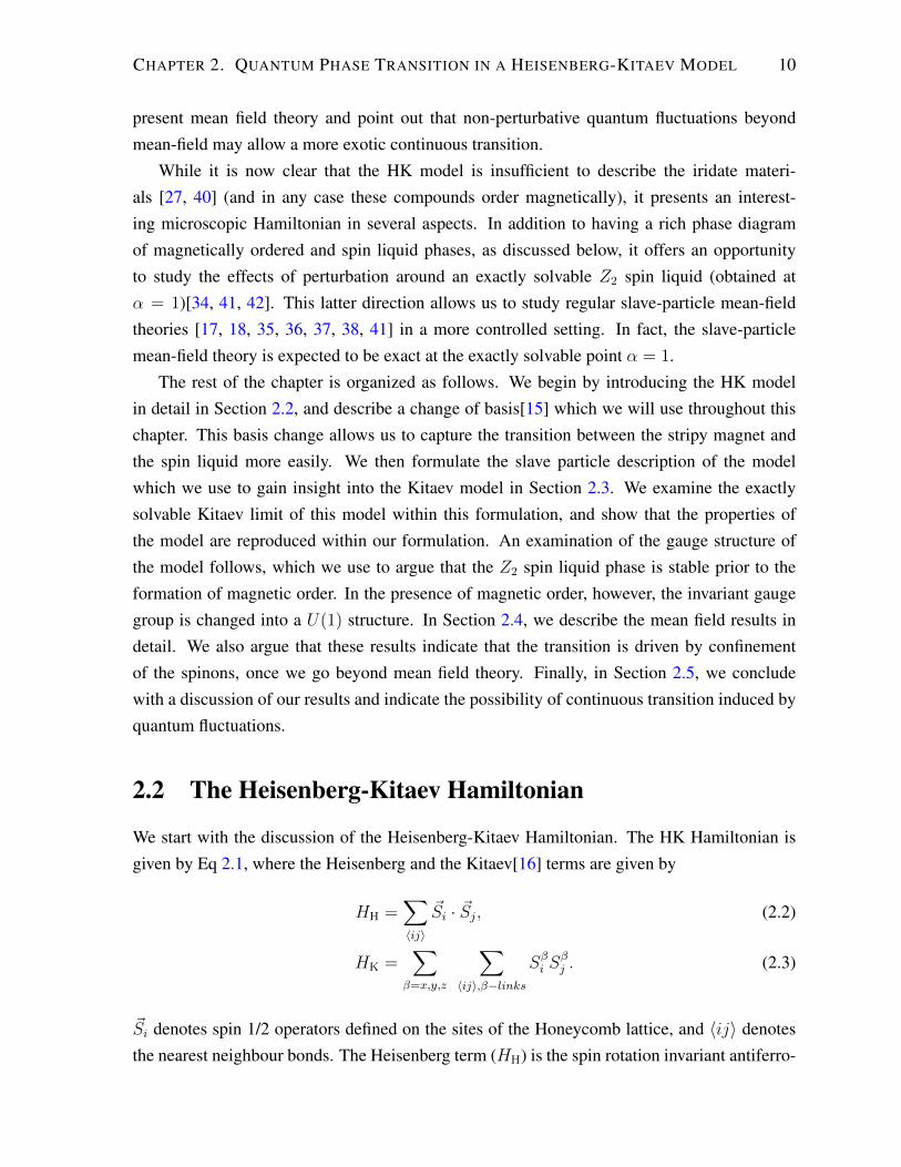
2.2 The Heisenberg-Kitaev Hamiltonian
We start with the discussion of the Heisenberg-Kitaev Hamiltonian. The HK Hamiltonian isgiven by Eq 2.1, where the Heisenberg and the Kitaev[16] terms are given by
HH =∑〈ij〉
~Si · ~Sj, (2.2)
HK =∑
β=x,y,z
∑〈ij〉,β−links
Sβi Sβj . (2.3)
~Si denotes spin 1/2 operators defined on the sites of the Honeycomb lattice, and 〈ij〉 denotesthe nearest neighbour bonds. The Heisenberg term (HH) is the spin rotation invariant antiferro-

CHAPTER 2. QUANTUM PHASE TRANSITION IN A HEISENBERG-KITAEV MODEL 11
0.0 0.4 0.8 1.0Α
Neel Stripy SL
(a)
(b)
(c)
Figure 2.1: (a) The Phase diagram for the Heisenberg-Kitaev model and the spin pattern in the(b) Neel and (c) Stripy phases.

CHAPTER 2. QUANTUM PHASE TRANSITION IN A HEISENBERG-KITAEV MODEL 12
Figure 2.2: The different interactions of the Kitaev model[16] where the x, y and the z bondsare shown. The black and the white circles denote the two sublattices A and B. ~Rx
AB =12
[1,−√
3]
and ~RyAB = 1
2
[1,√
3]
are the two unit vectors.
magnetic Heisenberg Hamiltonian, coupling spins on all nearest neighbour bonds. In contrast,the Kitaev term [16](HK) couples the x components of the spins on one of the directions ofbonds (referred to as x − links) on the honeycomb lattice, the y components of spins on they− links, and the z components on the z− links, as shown in Figure 2.2. More precisely, theKitaev model that we have written down is the isotropic Kitaev model where the couplings onthe x, y and z links are equal.[16]
The HK model does not have continuous spin rotation symmetry other than at the pointsα = 0 and 0.5. This stems from the Kitaev part of the Hamiltonian which is devoid of contin-uous spin rotation symmetry. At this point it is useful to note the important symmetries of theHK model, which are
1. 2π3
spin rotation about [111] spin axis along with C3 lattice rotations about any site.
2. Inversion about any plaquette center
3. Inversion about any bond center.
4. Time reversal.
The C3 symmetry ensures that there are three different stripy phases, which we will referto as the x, y and z stripy phases (see later). For the β(= x, y, z) stripy phase, the spins are

CHAPTER 2. QUANTUM PHASE TRANSITION IN A HEISENBERG-KITAEV MODEL 13
Figure 2.3: The rotated basis: the squares are left invariant, the circles are rotated about the zbonds, the triangles about the x bonds and the pentagons about the y bonds. This rotation wasfirst described by Khaliulin[44] and Chaloupka et al.[15]
oriented along the β axis, with the β links being ordered ferromagnetically and the remainingtwo links ordered antiferromagnetically. Figure 2.1c shows one of the three possible stripyphases, namely z stripy phase.
At the point α = 1, the model can be exactly solved by transforming the spins into productsof Majorana fermions, with a background of frozen Z2 fluxes over plaquettes[16]. This isa gapless Z2 spin liquid, with strictly nearest neighbour spin-spin correlations.[26] On theother hand, for α = 0 we have the pure spin rotation invariant nearest neighbour Heisenbergantiferromagnet where both numerical methods and semiclassical approaches give 2-sub-latticeNeel order.[43] In addition to these points, the model has another exactly solvable point atα = 0.5, where the stripy state is the exact ground state.[15, 44] This is easy to see by doinga selective rotation of the spins on the honeycomb lattice. It turns out that this rotated basis isuseful to describe the transition between the stripy phase and the spin liquid. Hence, we shallrecall the the essence of the rotation as pointed out by Khaliulin[44] and Chaloupka et al.[15]
2.2.1 The HK model in the rotated basis
The transformation of the spin basis required to reveal the exactly solvable point at α = 0.5
is described in figure 2.3. This transformation requires different spins to be rotated aboutdifferent axis, depending on their position in the lattice as described in the figure. We first

CHAPTER 2. QUANTUM PHASE TRANSITION IN A HEISENBERG-KITAEV MODEL 14
choose a set of spins which are positioned on third nearest neighbour sites at opposite cornersof the hexagons throughout the lattice, and hold these spins fixed. We next rotate the threespins that are adjacent to these fixed spins by π about the spin axis corresponding to the bondwhich connects it to the fixed spin. This has the net effect of transforming the Heisenberg termas
HH → −HH + 2HK (2.4)
and leaving the Kitaev term invariant, i.e.
HK → HK. (2.5)
From now on, we use spins in the rotated basis. However, for the sake of brevity, we shall con-tinue to use the same symbol for the spins and the Hamiltonians. In this basis, the Hamiltonian(given by Eq. 2.1) becomes
H → H = −(1− α)HH − 4(α− 1
2)HK. (2.6)
In this form, the exactly solvable point at α = 0.5 is clearly visible, as here the coefficient of theHK term is zero and this is simply the ferromagnetic Heisenberg model with a ferromagneticground state in terms of the rotated spins. On undoing the rotations we recover the stripy-antiferromagnetic ordering in terms of the un-rotated spins.[15, 44]
Since we wish to particularly examine the transition between the Kitaev spin liquid and thestripy anti-ferromagnetic state, we find it easier to use this rotated basis. Also, it is helpfulto think about deviations from the exactly solvable point at α = 0.5 in order to simplify thecouplings in the region of interest. We achieve this by introducing the parameter
δ = α− 1
2. (2.7)
This gives
H = −(1
2− δ)HH − 4δHK. (2.8)
Finally, we restrict ourselves to the region δ ∈ [0, 0.5] where these couplings are purely ferro-magnetic. We remind ourselves that δ = 0 now refers to the exact ferromagnetic state (or thestripy state in the original basis) while δ = 0.5 refers to the exactly solvable Kitaev point.
We take this rotated model as the starting point of our slave-particle analysis.

CHAPTER 2. QUANTUM PHASE TRANSITION IN A HEISENBERG-KITAEV MODEL 15
2.3 Slave Particle formulation
Having written down the Hamiltonian (Eq. 2.8) in the desired form, we now introduce theslave-particle decomposition of the (rotated) spins. We write the spin-1/2 operator as a bilinearof two spin-1/2 fermionic spinons as[17, 18]
Sµj =1
2f †jα[σµ]αβfjβ, (2.9)
where fjσ(σ =↑, ↓) are the fermionic spinon annihilation operators which satisfy regularfermionic anti-commutation relations. The above representation of the spin operators, alongwith the single fermion per site constraint
f †i↑fi↑ + f †i↓fi↓ = 1, (2.10)
constitutes a faithful representation of the spin-1/2 operators.[17, 18]The bilinear spin-spin interaction is a quartic term in the spinon operators. Within mean
field theory, we now seek to decouple these quartic spinon terms into stable decoupling chan-nels which are quadratic in terms of the spinons operators. In general, we need to keep boththe particle-hole and particle-particle channels for the spinons. [17]
However, we note that both the terms in the final Hamiltonian (Eq. 2.8) have ferromag-netic interactions. Thus the usual decoupling[17] in terms of the spin-singlet particle-hole andparticle-particle channels is unstable within a auxiliary field decoupling scheme. Instead, itwas shown by Shindou and Momoi[45] that the correct spin liquid decoupling scheme for suchinteractions is into the spin triplet channels (both particle-hole and particle-particle). This isdone as follows. We write the α-th component of the spin-spin interaction as
Sαi Sαi+p =
1
2
∑β=x,y,z
(1− δα,β)[Eβ†i,pE
βi,p +Dβ†
i,pDβi,p
]− ni
4, (2.11)
where δα,β = 1(0) for α = β(α 6= β) (not to be confused with the parameter δ) is the Kroneckerdelta function,
Eµi,p =
1
2f †i+pα[σµ]αβfiβ, (2.12)
Dµi,p =
1
2fi+pα[iσyσµ]αβfiβ (2.13)
and ni = 1 is the number of spinons per site.In addition to these hopping and pairing decouplings which capture the spin liquid, we

CHAPTER 2. QUANTUM PHASE TRANSITION IN A HEISENBERG-KITAEV MODEL 16
introduce a direct channel or magnetic decoupling,
mj =1
2〈f †jα[σz]αβfjβ〉, (2.14)
which, without loss of generality, we choose to be in the Sz direction. We include this de-coupling explicitly in order to access the ferromagnetic state and due to the fact that it is thecompeting order in the spin liquid phase. It is important to note that when this operator has anon-zero expectation value (in the unrotated basis) it explicitly breaks the the discrete symme-try corresponding to a lattice rotation by 2π
3about an individual site in conjunction with a spin
rotation by 2π3
about the [111] spin axis (refer to our discussion of the symmetries of the HKmodel).
Using the above general ansatz, the mean-field spinon Hamiltonian for the rotated HKmodel is given by
HHK = −(1
2− δ)HMF
H − 4δHMFK , (2.15)
where
HMFH =
1
4
∑i
∑p
(m(f †i,α[σz]αβfi,β + f †i+p,α[σz]αβfi+p,β)− 2m2 + (f †i,α
~Ei,p · ~σαβfi+p,β + h.c.)
− 2| ~Ei,p|2 + (f †i,α~Di,p · (−i~σσy)αβf †i+p,β + h.c.)− 2| ~Di,p|2
), (2.16)
HMFK =
1
4
∑i
∑p,r
(1− δp,r)(
(f †i,αEri,pσ
rαβfi+p,β + h.c.)− 2|Er
i,p|2
+ (f †i,αDri,p(−iσrσy)αβf
†i+p,β + h.c.)− 2|Dr
i,p|2]). (2.17)
Here i refers to the honeycomb lattice sites and p, r(= x, y, z) correspond to the link typesand spin components respectively. Eq. 2.17 is the most general mean field Hamiltonian withthe above decoupling channels.
Taking the Fourier transform and restricting the parameters ~E, ~D and m for each bond type

CHAPTER 2. QUANTUM PHASE TRANSITION IN A HEISENBERG-KITAEV MODEL 17
to have the symmetry of the lattice, we get
HMFH =2
∑k
((f †k,α,Aεαβ(k)fk,β,B + h.c.) + (f †k,α,A∆αβ(k)f †−k,β,B + h.c.)
)− Nsite
4
∑p
(| ~Ep|2 + | ~Dp|2) + 2∑k
∑η=A,B
f †k,α,ηΩαβfk,β,η −3Nsite
4m2, (2.18)
HMFK =2
∑k
((f †k,α,Aεαβ(k)fk,β,B + h.c.) + (f †k,α,A∆αβ(k)f †−k,β,B + h.c.)
)− Nsite
4
∑p,r
(1− δp,r)(|Erp|2 + |Dr
p|2), (2.19)
where Nsite is the number of lattice sites and we have defined the Fourier transform of thespinons as:
fk,α,L =1√N
∑Ri
eik·Rifi,α,L (2.20)
(N is the number of unit cells, α =↑, ↓ and L = A,B is the sub-lattice index) and alsointroduced
Ωαβ =3
8mσzαβ, (2.21)
εαβ(k) =1
8
∑p
ei~k·~RpAB ~Ep · ~σαβ, (2.22)
εαβ(k) =1
8
∑p,r
(1− δp,r)ei~k·~RpABEr
pσrαβ, (2.23)
∆αβ(k) =1
8
∑p
ei~k·~RpAB ~Dp · [−i~σσy]αβ, (2.24)
∆αβ(k) =1
8
∑p,r
(1− δp,r)ei~k·~RpABDr
p[−iσrσy]αβ, (2.25)
where we denote the unit lattice vectors (refer to figure 2.2) with
~RxAB = (
1
2,
√3
2), ~Ry
AB = (−1
2,
√3
2), ~Rz
AB = 0. (2.26)
We can write the above mean field Hamiltonian (Eq. 2.15) in a more compact way as aBogoliubov-de-Gennes Hamiltonian for the spinons using the 4-component Nambu spinons,
~f †i =[f †i,↑ f †i,↓ fi,↑ fi,↓
]. (2.27)

CHAPTER 2. QUANTUM PHASE TRANSITION IN A HEISENBERG-KITAEV MODEL 18
The mean field Hamiltonian can now be written as
HMF = C +∑i
∑p
(~f †i+pUi,p
~fi
− (1
8− δ
4)m(f †i,α[σz]αβfi,β + f †i+p,α[σz]αβfi+p,β)
),
(2.28)
where
C =Nsite
4
(3m2(
1
2− δ) +
∑p,r
[(1
2− δ) + 2δ(1− δp,r)]
× (|Erp|2 + |Dr
p|2))
(2.29)
and
Ui,p =1
8
∑r
(− (
1
2− δ)− 4δ(1− δp,r)
)(Er†i,pσ
r(τ3 + τ0) + Eri,p(σ
r)T (τ3 − τ0)
+Dr†i,p(iσ
yσr)τ− −Dri,p(iσ
y(σr)T )τ+).
(2.30)
Here the σ matrices are Pauli matrices operating on the spin indices and the τ matrices arePauli matrices operating on the particle-hole indices (τ0 is the identity matrix in the particle-hole space). For the sake of clarity of notations, we have suppressed the sub-lattice index.
We now re-write the Fourier transform of the above Hamiltonian in a Nambu form to get
HMF = C +∑k
∑α,β
~α†kαHk,αβ~αkβ, (2.31)
where C is defined by Eq. 2.29 and we have now used the 4-component spinors
~α†k,β =[f †k,A,β f †k,B,β f−k,A,β f−k,B,β
], (2.32)
A,B refer to the two sublattices of the honeycomb lattice (as shown in figure 2.2), β =↑, ↓denotes the spin and Hk,αβ is given by
Hk,αβ =
(1
2− δ)Ωαβ ξαβ(k) 0 Γαβ(k)
[ξβα(k)]∗ (12− δ)Ωαβ −Γβα(−k) 0
0 −[Γαβ(−k)]∗ −(12− δ)Ωαβ −[ξαβ(−k)]∗
[Γβα(k)]∗ 0 −ξβα(−k) −(12− δ)Ωαβ
. (2.33)

CHAPTER 2. QUANTUM PHASE TRANSITION IN A HEISENBERG-KITAEV MODEL 19
We have used the following notations
ξαβ(k) = −1
2(1− 2δ)εαβ(k)− 4δεαβ(k), (2.34)
Γαβ(k) = −1
2(1− 2δ)∆αβ(k)− 4δ∆αβ(k).
For a given spin liquid ansatz, we diagonalize the matrix Hk as ρkDkρ†k, define the vector
~γk = ρ†k~αk and determine the values of the mean field parameters Eµp , Dµ
p and mj .
To obtain the self consistent solution, we begin with an ansatz consistent with magneticordering and with a combination of hopping and pairing decouplings, and allow the sys-tem to evolve to a fixed point by self-consistent iteration on the values of the mean fieldparameters[46]. As all the mean field parameters are quadratic in the fermionic variables,each step in the iteration process requires an evaluation of the expectation values of quadraticfermion operators in the ground state, which are re-calculated iteratively to obtain the self-consistent solution.
This brings us to the spin liquid ansatz which we describe next.
2.3.1 The Spin Liquid Ansatz
In general we have a nineteen-parameter mean field model which needs to be solved self-consistently. These fields are:
On p− links : Exi,p, E
yi,p, E
zi,p, D
xi,p, D
yi,p, D
zi,p (2.35)
(where p = x, y, z) and the on-site magnetization mi. In the spin liquid regime, the magnetiza-tion is zero and we have eighteen complex parameters and the magnetization. A self consistentmean-field analysis in terms of this eighteen(+ one) parameter model suggests that the stablemean-field states that we find involve only nine parameters or their gauge equivalent forms, inaddition to magnetization in one phase. Thus we study this nine (+ magnetization) parametermodel which captures both the spin liquid and the magnetically ordered ground states. Thenumerical calculations can further be simplified by a correct choice of gauge. To this end, weuse insights from the exact solution of the Kitaev model.[16] This, as shown below, can beobtained by choosing the following form for the nine parameters:
On p− links : Dxi,p, E
zi,p ∈ Imaginary, (2.36)
Dyi,p ∈ Real, (2.37)
CHAPTER 2. QUANTUM PHASE TRANSITION IN A HEISENBERG-KITAEV MODEL 20
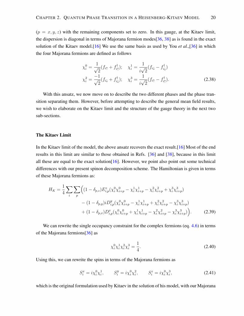
(p = x, y, z) with the remaining components set to zero. In this gauge, at the Kitaev limit,the dispersion is diagonal in terms of Majorana fermion modes[36, 38] as is found in the exactsolution of the Kitaev model.[16] We use the same basis as used by You et al.,[36] in whichthe four Majorana fermions are defined as follows
χ0i =
1√2
(fi↑ + f †i↑); χ1i =
1
i√
2(fi↓ − f †i↓)
χ2i =−1√
2(fi↓ + f †i↓); χ3
i =1
i√
2(fi↑ − f †i↑). (2.38)
With this ansatz, we now move on to describe the two different phases and the phase tran-sition separating them. However, before attempting to describe the general mean field results,we wish to elaborate on the Kitaev limit and the structure of the gauge theory in the next twosub-sections.
The Kitaev Limit
In the Kitaev limit of the model, the above ansatz recovers the exact result.[16] Most of the endresults in this limit are similar to those obtained in Refs. [36] and [38], because in this limitall these are equal to the exact solution[16]. However, we point also point out some technicaldifferences with our present spinon decomposition scheme. The Hamiltonian is given in termsof these Majorana fermions as:
HK =1
4
∑i
∑p
((1− δp,z)Ez
i,p(χ0iχ
0i+p − χ1
iχ1i+p − χ2
iχ2i+p + χ3
iχ3i+p)
− (1− δp,y)iDyi,p(χ
0iχ
0i+p − χ1
iχ1i+p + χ2
iχ2i+p − χ3
iχ3i+p)
+ (1− δp,x)Dxi,p(χ
0iχ
0i+p + χ1
iχ1i+p − χ2
iχ2i+p − χ3
iχ3i+p)). (2.39)
We can rewrite the single occupancy constraint for the complex fermions (eq. 4.6) in termsof the Majorana fermions[36] as
χ0iχ
1iχ
2iχ
3i =
1
4. (2.40)
Using this, we can rewrite the spins in terms of the Majorana fermions as
Sxi = iχ0iχ
1i , Syi = iχ0
iχ2i , Szi = iχ0
iχ3i , (2.41)
which is the original formulation used by Kitaev in the solution of his model, with our Majorana

CHAPTER 2. QUANTUM PHASE TRANSITION IN A HEISENBERG-KITAEV MODEL 21
fermions normalized such that χαi , χβj = δijδ
αβ . A set of plaquette operators,
Wp = 26Sx1Sy2S
z3S
x4S
y5S
z6 , (2.42)
are defined on the individual plaquettes of the lattice, where the sites 1−6 traverse a honeycombplaquette as shown in figure 2.2. (The factor of 26 which is present in our definition of Wp isdue to the plaquette operator being written in terms of spins, rather than Pauli matrices as inthe original formulation of Kitaev.[16]) These plaquette operators commute with the originalKitaev spin Hamiltonian and with one another, which allows the Hilbert space to be split intoeigen-spaces of these operators, enabling the exact solution. These operators do not commutewith the mean field Hamiltonian; however, that these operators take the same value in themean-field solution as in the exact solution.[38]
To make a connection with Kitaev’s original solution we now express our results in termsof the Majorana fermions. By construction, the Majorana fermions introduced in Eq. 2.38 arethe modes in which the band structure is diagonal. While χ1, χ2 and χ3 form the flat bands,the single dispersing band is made up of the χ0 fermions.[36] In terms of the original solutionof Kitaev, the dispersing fermion is the single gapless Majorana mode, while the flat bandfermions describe the frozen Z2 fluxes, as we now show. The flat bands arise from the factthat the mean-field Hamiltonians for χ1, χ2 and χ3 become disjoint, i.e., the hopping for thesefermions are non-zero only on x, y or z bonds respectively. For the hopping on the z-link, wehave,
Ξ(iχ3iχ
3j − iχ3
jχ3i ) (2.43)
where Ξ is expressed in terms of the mean field parameters and ij are neighbours on a z-link.The eigenvalues are given by ±|Ξ|, independent of ~k, and therefore these form the flat bands.At half filling, the lower energy state (lower flat band) is occupied. To compare with the exactsolution, the Majorana bilinear χ3
iχ3j has to be identified with the Z2 gauge fields defined on
the z-links, uzij .[16] Indeed, we identify
uzij = 2iχ3iχ
3j = i(χ3
iχ3j − χ3
jχ3i ). (2.44)
In the ground state, clearly the eigenvalues of uzij are ±1. Similarly we can introduce uxij anduyij on x and y links respectively. Now we can re-write the flux operators Wp in Eq. 2.42 (using2.41, 2.40 and the fact that χαi χ
αi = 1
2) as
Wp = 26Sx1Sy2S
z3S
x4S
y5S
z6 = uz12u
x23u
y34u
z45u
x56u
z61 (2.45)

CHAPTER 2. QUANTUM PHASE TRANSITION IN A HEISENBERG-KITAEV MODEL 22
It is now clear that in the ground state the plaquette operators Wp have an expectation valueof +1. For a small departure from this Kitaev point, one can still use the variables upij andWp. However, these are no longer static, but acquire dynamics as the corresponding Majoranafermions starts dispersing.
The fermionic mean-field theory of this state describes a Z2 spin liquid, as we will showexplicitly in the next subsection. At the mean field saddle-point, the values of different param-eters are given by
− iDyi,x = Ez
i,x = Dxi,y = Ez
i,y = Dxi,z = −iDy
i,z = 0.190608i,
Dxi,x = −iDy
i,y = Ezi,z = −0.0593918i, (2.46)
values which have been determined by self-consistent iteration[46], as described above.
The resultant spinon spectrum is given in Figure 2.4. There are 8 bands which, characteris-tic of Bogoliubov Hamiltonians, are symmetric about zero energy. The flat bands are threefolddegenerate. At half filling for the spinons the lower four bands (red) are filled while the upperfour bands (blue) are empty. While the flat bands are gapped, the two dispersing bands meetat the boundary of the hexagonal Brillouin zone with a characteristic Dirac spectrum. Hencethe spin liquid that we are describing is indeed gapless and matches with the spinon spectrumobtained in the exact solution of the Kitaev model. This provides a useful check on the validityof our mean field solution, as well as a controlled limit from which we can perturb the model.
The presence of the pairing term indicates that, in terms of the complex fermions, thespin liquid is a “superconductor” for the spinons. We can analyze the symmetry of the pairingamplitude. In order to determine the properties of the pairing around the Dirac node, we isolatethe dispersing band by examining the χ0 fermionic modes and returning to the original basisof Dirac fermions. For the χ0 modes, the Hamiltonian is given by
H0K =
M
4
∑i
∑p
χ0iχ
0i+p (2.47)
=M
8
∑i
∑p
(fi,↑ + f †i,↑)(fi+p,↑ + f †i+p,↑)
=1
8
∑k
∑p
(M(fk↑Af−k↑B + fk↑Af†k↑B)e−i
~k·~RpAB + h.c.) (2.48)
where M = 0.38122i. From here we can expand the pairing terms about the K-points in the

CHAPTER 2. QUANTUM PHASE TRANSITION IN A HEISENBERG-KITAEV MODEL 23
brillouin zone. Defining ~k′ = ~k + (2π3, 2π√
3),
∆dispersing(k′) =
M
8(1 + e
4πi3 e−i
~k′·~RxAB + e2πi3 e−i
~k′·~RyAB)
≈ M√
3
16(−k′x + ik′y). (2.49)
However, we would like to emphasize that the above chiral p-wave pairing does not necessar-ily imply time-reversal symmetry breaking, which is now implemented projectively.[17] Thestructure of the pairing terms differs from the work of Burnell and Nayak [38], who found pypairing about the Dirac points, by choosing a different basis for the fermions which is relatedto the present one by a gauge transformation.
We can further calculate the spin-spin correlation functions within mean field theory. Usingthe Majorana representation we find that this is given by:
〈Sαi Sβj 〉 ∼ 〈χ0
iχ0j〉〈χαi χ
βj 〉 (2.50)
Since the second correlation function involves absolutely flat bands, it is only non-zero whenα = β and when i = j or i and j belong to the same unit cell. Hence the spin correlationare short ranged even if the spin liquid is gapless. This is a novel feature of the Kitaev spinliquid, where exact calculations[26] also indicate that such correlations vanish beyond nearestneighbour.
We would like to point out here that, when the model is perturbed with the Heisenberg term,the gapped flat bands acquire a weak dispersion, but still remain gapped. Within perturbationtheory, this is expected to lead to exponentially decaying spin-spin correlation decaying with alength-scale characteristic of the energy-gap.[41]
2.3.2 The gauge structure
At this point, before actually discussing the results of our mean-field calculations, we wish todiscuss the gauge structure of the our spin liquid ansatz.
While the formulation outlined above is more suited to calculations of the mean field spec-trum and self-consistent solutions, to decipher the nature of the spin liquid and the gaugetransformations we wish to cast the above decoupling within an SU(2) formalism.
In order to examine the nature of the spin liquid state, it is worthwhile to formulate thisHamiltonian in another basis. The transformation into this basis is defined by
~fi → ~f ′i = A~fi, Ui,p → AUi,pA†, (2.51)

CHAPTER 2. QUANTUM PHASE TRANSITION IN A HEISENBERG-KITAEV MODEL 24
-0.3
-0.2
-0.1
0
0.1
0.2
0.3
Γ M K Γ
Figure 2.4: (Color online) Spinon spectrum in the Kitaev limit. Bands shown in red are occu-pied, bands shown in blue are unoccupied.
where the transformation matrix is given by
A =
1 0 0 0
0 0 0 1
0 1 0 0
0 0 −1 0
(2.52)
and ~fi is given by Eq. 2.28. In the new basis, the ~f ′i are given by
~f ′i† =
[f †i,↑ fi,↓ f †i,↓ −fi,↑
]. (2.53)
In this basis, we can write the set of gauge transformations which leave our physical spindegrees of freedom invariant in a block diagonal form,
Wi =
[Vi 0
0 Vi
](2.54)
where the Vi matrices form a two dimensional representation of SU(2). The spinon Hamil-tonian (Eq 2.31), when written in the new basis, is invariant under the simultaneous gauge

CHAPTER 2. QUANTUM PHASE TRANSITION IN A HEISENBERG-KITAEV MODEL 25
transformation
~f ′i → Wi~f ′i , U ′i,p → Wi+pU
′i,pW
†i . (2.55)
where U ′i,p = AUi,pA† gives the analog of Bogoliubov-de-Gennes Hamiltonian in the new
basis.
In order to study the low energy degrees of freedom in this theory, we allow gauge fluctua-tions of the U ′i,p matrices of the form
U ′i,p = U ′i,peiali,pκ
l
, (2.56)
where these κl matrices are block diagonal four by four matrices
κl =
[ηl 0
0 ηl
], (2.57)
where the ηl are Pauli matrices which act on the gauge degree of freedom, and generate ourgauge transformations. We also take note of a set of matrices which generate our spin rotationalsymmetry, which in this basis are given by
Σl = σl ⊗ I, (2.58)
where the σl are again Pauli matrices, acting on the spin degrees of freedom of our fermions.
To determine the gauge structure, we now consider the product of the U ′i,p matrices arounddifferent lattice loops based at any site i,[17]
P (Ci) =∏C
U ′i,p (2.59)
Here the product is taken over the bonds of the loop Ci, beginning and ending at the site i.Using the given notations, we can write our U ′i,p matrices as
U ′i,p = ξαβΣακβ (2.60)
where Σα = (Σ0,Σ1,Σ2,Σ3), κβ = (κ0, κ1, κ2, κ3) (Σ0 and κ0 are 4 × 4 identity matricesand the other matrices are given by Eqs. 2.57 and 2.58), and the ξαβ are complex numbers.We note that, unlike the singlet case, in the triplet decoupling scheme both the gauge and thespin generators enter in U ′i,p. (In other words, in the singlet decoupling[17] Σ0 is the only spingenerator that enters since the decoupling channels are invariant under spin rotations).

CHAPTER 2. QUANTUM PHASE TRANSITION IN A HEISENBERG-KITAEV MODEL 26
Similarly the loop function can be written as
P (Ci) = ξαβΣακβ (2.61)
where the ξαβ are determined by the values of the ξαβ on the links of the loop Ci.
If all the loop functions, based at any site, can be rotated into a form which commutes withone or more gauge generators, then the set of such generators form the invariant gauge group(IGG) and the low energy gauge fluctuations belong to the IGG.[17]
Taking our ansatz in the Kitaev limit of the model, the structure of the U ′i,p matrices is givenby
U ′i,p = −Rκ3Σ3 + iQκ2Σ2 + Pκ1Σ1, (2.62)
where
R =1
4(1− δp,z)Ez
i,p, P =1
4(1− δp,x)Dx
i,p,
Q =1
4(1− δp,y)Dy
i,p. (2.63)
The loop functions in this limit (in our choice of gauge) have a typical structure which is givenby
P (Ci) = T (κ0Σ0 − κ1Σ1 + κ2Σ2 + κ3Σ3), (2.64)
where T is a constant. We find that these cannot be brought into a form which commutes withany of the gauge generators, and hence the only kind of low energy gauge fluctuation allowedhas the form Wi = eiεiκ
l where εi = 0 or π. This gives an IGG≡ Z2 and we have a Z2
spin liquid. This spin liquid has gapless Majorana excitations (see previous sub-section) andis indeed the Kitaev spin liquid. This IGG survives throughout the entire regime of δ in whichmagnetic order is absent. This completes our discussion regarding the invariant gauge groupof the gapless spin liquid, which we have now shown to be Z2, as expected from Kitaev’s exactsolution.[16]
However, in the presence of magnetic ordering the above picture is no longer true. Magneticorder drives the Ez
i,p parameter to zero, which changes these U ′i,p matrices into a form given by
U ′i,p = iQκ2Σ2 + P κ1Σ1, (2.65)

CHAPTER 2. QUANTUM PHASE TRANSITION IN A HEISENBERG-KITAEV MODEL 27
where
P =1
8[(
1
2− δ) + 4δ(1− δp,x)]Dx
i,p, (2.66)
Q =1
8[(
1
2− δ) + 4δ(1− δp,y)]Dy
i,p. (2.67)
The loop functions are now given by
P (Ci) = T (κ0Σ0 + κ3Σ3), (2.68)
where T is a different constant. It is now easy to show that the κ3 matrix commutes withthese products, and the gauge transformations of the form Wi = eiθiκ
3(θi ∈ [0, 2π)) leave
our ansatz invariant. Thus, in this case, the IGG≡ U(1) and hence the low energy gaugefluctuations are described by a compact U(1) gauge theory which has a gapless photon andalso instantons (space-time monopoles) where the gauge flux may change in integral multiplesof 2π. In addition, using the gauge transformation
~f ′i,B →
[iσy 0
0 iσy
]~f ′i,B, U ′i,p →
[iσy 0
0 iσy
]U ′i,p (2.69)
the Dij can now be completely rotated into the Eij vectors (when Ei,p is zero) hence explicitlyshowing that this is a U(1) spin liquid. Later, we shall see that the spinon spectrum is gapped(in the presence of magnetic ordering), and that this state is actually a gapped U(1) spin liquidwhich is unstable to confinement in two spatial dimensions. This significance of this instabilitywill be discussed later.our
2.4 The results of the mean field theory and beyond
We now discuss the results of our mean field calculations as a function of δ. These meanfield results are obtained by solving the self-consistent equations for the various mean fieldparameters.
Region surrounding the Kitaev limit (δ ≈ 0.5): Near the Kitaev limit, we find that thespinon bands which were flat in the pure Kitaev limit gain a dispersion, with energy whichscales with the distance from the exactly solvable point. These bands do not contribute sig-nificantly to the low energy theory due to the fact that they remain fully gapped, and the lowenergy spinon excitations remain consistent with those of the pure Kitaev model. Figure 2.5ashows the band structure in this region, at the value of δ = 0.3. As the strength of the Heisen-

CHAPTER 2. QUANTUM PHASE TRANSITION IN A HEISENBERG-KITAEV MODEL 28
-0.2
-0.15
-0.1
-0.05
0
0.05
0.1
0.15
0.2
Γ M K Γ(a)
-0.15
-0.1
-0.05
0
0.05
0.1
0.15
Γ M K Γ(b)
Figure 2.5: (a) The spinon band structure for the Heisenberg-Kitaev model with nonzeroHeisenberg coupling and zero net magnetization, at the point δ = 0.3. (b) The spinon bandstructure for the Heisenberg-Kitaev model with nonzero Heisenberg coupling and non-zero netmagnetization, at the point δ = 0.23.

CHAPTER 2. QUANTUM PHASE TRANSITION IN A HEISENBERG-KITAEV MODEL 29
berg coupling is increased, the mean field parameters show only a slight change prior to theonset of magnetic ordering.
Region with non-zero magnetic order (δ ≤ 0.26): At δ ≈ 0.26, we find that the system be-gins to admit a non-zero magnetic order parameter as a self-consistent solution. The magneticorder parameter jumps discontinuously to a finite value at this point, indicating a first orderphase transition. The spinon band structure differs significantly in this phase, which includesthe formation of a band gap. Figure 2.5b shows a cut of the spinon bands in this region, at thevalue of δ = 0.23. We also note that the values of all of the mean field parameters are changedby this ordering, and that the value of the hopping order parameters are driven to zero. Aswe continue to increase the strength of the Heisenberg coupling (decrease δ) we see that themagnetic order parameter is increased, and the pairing amplitudes are driven to zero as well(below δ ≈ 0.15). Once the pairing amplitudes are zero, all the spinon bands become flat (notshown) and also have an energy gap.
The self-consistent values of the different mean field parameters are plotted in figure 2.6.This shows that the magnetic order parameter discontinuously turns on at δ ≈ 0.26. Below thisvalue of δ there is finite magnetic order. Also at that value of δ, Ez
ij goes to zero discontinu-ously.
2.4.1 Interpretation of mean field results
As discussed, for δ ≥ 0.26 (i.e. α ≥ 0.76) there is no magnetic order and the Ei,p and Di,p
fields are non-zero. This, as we have already discussed already, is a Z2 spin liquid which iscontinuously connected to the exactly solvable kitaev spin liquid (obtained for α = 1). Thishas gapless Majorana fermion excitations and short range spin correlations.
On the other hand, for δ ≤ 0.26 there is magnetic order. However, at the mean fieldlevel spinon bands are well defined and there are dispersing spinons. Only the Di,p fieldsare non-zero in this phase. However, we have already shown (see Eq. 2.69) that these Di,p
fields can be gauge rotated into Ei,p fields and hence this regime represents a U(1) spin liquid.Since the spinon band structure is gapped, we essentially have a gapped U(1) spin liquid withferromagnetic order. We can call this phase a FM∗ in order to distinguish it with the regularferromagnetic order. In addition to the gapped fermionic spinon excitations, there is a gaplessemergent U(1) gauge photon present in this phase. This arises from the underlying U(1) gaugefluctuations that this phase allows. However, contrary to our regular electrodynamics, thisemergent U(1) gauge group is compact[17]. Hence, as noted earlier, in addition to the photon,it allows instanton processes where the magnetic flux changes by integral multiple of 2π. This

CHAPTER 2. QUANTUM PHASE TRANSITION IN A HEISENBERG-KITAEV MODEL 30
-0.1 0
0.1 0.2 0.3 0.4 0.5 0.6 0.7 0.8
0 0.1 0.2 0.3 0.4 0.5
δ
m
Dixx ,Diy
y
Dixy ,Diy
x
Dizx ,Diz
y
Eixz ,Eiy
z
Eizz
Figure 2.6: (Color online) The magnitude of the mean field parameters, plotted as a function ofδ. The onset of magnetic order triggers a first order phase transition. The symbols are a guidefor the eye.
turns out to be significant, as we discuss in the next subsection. We also point out that ingeneral the FM∗ phase has a Goldstone mode (spin wave) that is in general gapped because thespin-rotation symmetry is broken explicitly (except at the points δ = 0 and δ = 0.5).
Since within mean field theory magnetic order turns on discontinuously, the transition isfirst order within the limits of our numerical resolution. The jump is about 20% of the saturationvalue. Hence, within mean field theory, we have a first order transition between the Z2 spinliquid with gapless spinons with Dirac dispersion to a FM∗ phase with gapped spinons.
2.4.2 Beyond mean field theory: Instantons and confinement of FM∗
In this sub-section, we discuss the issue of instability of the FM∗ phase to a conventional fer-romagnetic phase. As already pointed out, the compact U(1) gauge theory that describes thelow energy excitations of the FM∗ phase allows tunnelling processes where the magnetic fluxchanges (instanton events). It is known from the work of Polyakov[39] that in (2 + 1) dimen-sional compact U(1) gauge theory, when the matter fields carrying electric charges(spinons)are gapped, the instanton events are always relevant. Thus, once we incorporate fluctuations toour mean field solutions, we have to take into account the effect of such tunnelling processes.

CHAPTER 2. QUANTUM PHASE TRANSITION IN A HEISENBERG-KITAEV MODEL 31
Once such instanton events are taken into account, the spinons, which carry gauge charges, areconfined to gauge neutral objects– the spins. This confinement is not, however, a straightfor-ward consequence of magnetic order, as a stable gapless U(1) phase with deconfined spinonsand coexisting magnetic ordering can occur in two spatial dimensions[47, 48, 49]. We empha-size that it is the U(1) gauge structure of the magnetically ordered phase, combined with thegapped nature of the spinon excitations,[39] which is responsible for the confinement throughthe proliferation of instanton events.
The above discussion indicates that once we move beyond mean field theory and take theinstantons of the compact U(1) gauge theory into account, the spinons in the FM∗ phase un-dergo confinement. However, the ferromagnetic order parameter would survive due to the factthat it is gauge invariant. Such a confined phase is continuously connected to the regular fer-romagnetic phase for the spins and we end up with a FM phase (or the stripy phase for theunrotated spins). Thus, we indeed get a direct transition from the Z2 spin liquid to a stripyphase, albeit discontinuously.
2.5 Discussion
We now summarize the results of this chapter. We have obtained a slave-particle description ofthe HK model and used it to describe the phase transition between a spin liquid and the mag-netically ordered stripy phase within slave particle mean field theory. In the Kitaev limit of themodel, we have shown that this formulation reproduces the expected excitation spectrum andthat the plaquette operators which enable the exact solution are in a vortex free configurationin the ground state. Upon the inclusion of a small non-zero Heisenberg term we have founda similar low energy theory, although the bands which are dispersion-free in the Kitaev limitgain a dispersion. We have analyzed the gauge structure of the model, and have seen that inthe absence of magnetic order the Z2 IGG which describes the Kitaev spin liquid state remainsthe IGG of our ansatz. The magnetically ordered phase that we get by destroying the Z2 spinliquid is, within mean field theory, a gapped U(1) spin liquid which has stripy magnetic order.However, existing results imply that such a spin liquid is unstable to confinement, which im-mediately drives a transition to the regular stripy antiferromagnetic phase. Within mean-fieldtheory, the above transition turns out to be discontinuous. Our description allows for a coher-ent description of the spin liquid and the magnetically ordered phase as well as of the phasetransition connecting them.
The present numerical results[15, 34] cannot conclusively shed light on the nature of theabove transition between the spin liquid and the stripy antiferromagnet. However, these resultsseem to suggest that the transition is either continuous or weakly first order. While our mean

CHAPTER 2. QUANTUM PHASE TRANSITION IN A HEISENBERG-KITAEV MODEL 32
field theory indicates a first order transition, we are required to incorporate quantum fluctua-tions beyond the mean field to address the issue of a possible continuous transition betweenthe phases. In fact it is somewhat easy to see why the transition appears to be first order inour present calculations. Once we neglect the gauge fluctuations, we can treat the fields Eij
and Dij as “order parameters” along with the actual magnetization order parameter mi. ALandau-Ginzburg theory in terms of these fields can then be obtained by integrating out thefermions. Such a “multi-order parameter” Landau-Ginzburg theory with repulsive interactionsbetween the order-parameter densities generically gives a first order transition within mean-field theory.[50] Hence, the results of our mean field calculations can be understood withinthis framework. However, a shortcoming of such a naive Landau-Ginzburg analysis is the factthat it cannot take into account the effect of gauge fluctuations. Once such fluctuations are ac-counted for, the Eij and Dij fields can no longer be treated as order parameters, since they arenot gauge invariant, and so the above naive Landau-Ginzburg theory breaks down. This opensup the possibility of subtle gauge fluctuation effects driving this transition to second order. It isknown from earlier studies in frustrated magnets that such “Landau forbidden” generic contin-uum quantum phase transitions may occur (e.g. deconfined quantum critical points[51]) wherenaive mean field considerations break down or do not apply, since there are no local order pa-rameters (e.g. Topological phase transitions[52]). Hence such a second order transition wouldbe unconventional and potentially interesting, particularly in context of the the possibility ofrealizing the HK model in material systems.[15, 28] Similar transitions in spin rotation invari-ant systems have been recently studied both numerically[53, 54] and from the field theoreticalperspective.[55]

Chapter 3
Three-dimensional honeycomb iridates
In this chapter, we will examine the recent experimental motivation and theoretical work on thetri-coordinated iridate materials A2IrO3 and the associated models, with a focus on the three-dimensional Li2IrO3 compounds. These systems exemplify the physics of spin-orbit couplingand have drawn considerable recent interest as a result. In particular, the anisotropic nature ofthe spin exchange interactions is critical to the physics in these systems; as we will see, thisgives rise to fascinating phases of matter which depend on the strong SOC for their presence.
Bond-anisotropic models have been continually studied in literature even before the re-cent discoveries of iridate materials. The general class of models known as compass modelsare an example of such, where the pseudospins interact in a directionally-dependent mannerand can represent degrees of freedom like orbitals, vacancy centers, or even atomic states incold atom systems.[56] Similar to these compass models is the Kitaev model on the honey-comb lattice,[16] which is of particular significance to the iridate materials. This anisotropicspin-1/2 model can be exactly solved to reveal a spin-liquid ground state that can be used toperform fault-tolerant topological quantum computation.[57] The relation of the Kitaev modelto iridate materials was first elucidated by the seminal work of Jackeli and Khaliullin[58]: us-ing a perturbative calculation in the strong coupling limit, these authors invigorated the field byconjecturing that the honeycomb iridate Li2IrO3 can potentially realize the Kitaev model andits spin liquid ground state. However, both Li2IrO3 and its isoelectronic cousin Na2IrO3 havebeen found to order magnetically[29, 31, 59, 60] and subsequently many studies have soughtan explanation for the presence of magnetic order in place of a quantum spin-liquid groundstate.[61, 62]
Crystal distortions and further neighbour interactions in these quasi two-dimensional (2D)honeycomb iridates have been implicated as two possible causes for the observed magneticordering.[35, 63, 64, 65, 66] If true, the Kitaev spin liquid ground state may be difficult torealize in these materials since a controlled elimination of these effects is beyond the reach of
33

CHAPTER 3. THREE-DIMENSIONAL HONEYCOMB IRIDATES 34
current experimental techniques. It was, therefore, a welcomed development when two three-dimensional honeycomb-like iridates were independently and simultaneously discovered in2013.[67, 68] These two materials, the hyperhoneycomb iridate β-Li2IrO3 and the stripyhon-eycomb iridate γ-Li2IrO3, are polymorphs of the quasi 2D A2IrO3. Not only are they theoret-ically compatible with the Kitaev model and an extension of its exact spin-liquid ground statesolution, their fully three-dimensional lattice structure induces physics that is distinct fromtheir two-dimensional counterparts. In addition, the limited experimental viability of studyingiridium-based materials using neutron scattering[31] have pushed researchers to refine reso-nant x-ray scattering probes,[60, 69] which was used to characterize the ground states of these3D iridates in unparalleled detail.
Like their 2D counterparts, these 3D honeycomb iridates magnetically order, and are thusnot examples of a quantum spin liquid. However, studies have indicated that their interactionsmy be near the Kitaev limit in which quantum spin liquid behaviour would arise, and pressureexperiments on β-Li2IrO3 have eliminated the magnetic ordering, possibly pushing this mate-rial into a spin liquid state. It is worthwhile, then, to examine the compounds β-Li2IrO3 andγ-Li2IrO3 in more detail. We set the stage of discussion by first describing the crystal structureand experimental signatures of β-Li2IrO3 and γ-Li2IrO3. Next, we construct a microscopic un-derstanding of iridates by examining the nature of their spin-orbital entangled wavefunctions,which will enable us to investigate the anisotropic interactions between them. We will thenexplore the Kitaev model on these 3D lattices with an emphasis of how they differ from their2D counterpart.
3.1 Crystal structure and experimental signatures
The hyperhoneycomb β-Li2IrO3 and stripyhoneycomb γ-Li2IrO3 are both fully three-dimensionalcrystal structures as shown in Fig. 3.1. Determined by single crystal X-ray analysis, both ma-terials are orthorhombic: the former is in the face-centred space group Fddd (No. 70), thelatter is in the base-centred space group Cmmm (No. 66). They have similar lattice constants,and both contain the same number of atoms in their conventional unit cells. The basic buildingblock present in both structures is the IrO6 octahedron: these octahedra are tri-coordinated
(each have three nearest-neighbours) and adjacent octahedra are edge-shared (they have twooxygen atoms in common). Depending on how these building blocks are arranged in the crys-tal, a variety of structures—including the 2D honeycomb iridates—can be constructed.
To describe the arrangement of octahedra in these various structures, we first note that thereare several ways to orient a tri-coordinated and edge-shared cluster of four octahedra even if we

CHAPTER 3. THREE-DIMENSIONAL HONEYCOMB IRIDATES 35
stipulate that the octahedral axes are aligned with a set of global axes.1 In the 2D honeycombiridates, the orientation of these clusters ensure that all iridium sites are coplanar, resulting in atwo-dimensional layer that forms the real crystal structure when stacked. In the 3D honeycombiridates, there exists six-octahedra clusters where the middle bond twists, as demonstrated inFig. 3.1. These twists only occur along bonds that are parallel to the orthorhombic c direction(hereafter we call these the z-bonds), hence both 3D structures possess zigzag chains similarto the 2D honeycomb lattice. The difference between the two 3D lattices is the frequency ofthe bond twists: in β-Li2IrO3, they happen at every z-bond, while in γ-Li2IrO3, these twistshappen at every other z-bond. The resulting hyperhoneycomb lattice does not possess anyhexagons and the smallest loop of iridium sites contains ten ions. On the other hand, the stripy-honeycomb lattice does possess strips of hexagons. This construction of the crystal structuresenable the generalization of a family of polymorphs of Li2IrO3 called the harmonic honeycomb
series, denoted as 〈n〉-Li2IrO3, where n indicates the number of bonds between adjacent bondtwists. In this nomenclature, β-Li2IrO3, γ-Li2IrO3, and α-Li2IrO3 are 〈0〉-, 〈1〉-, 〈∞〉-Li2IrO3
respectively.[67]
Although the Li2IrO3 compounds can be represented by iridium atoms lying in the centerof oxygen octahedra in an ideal structure, deviations from this simple model are present. Inparticular, deviations in the bond length between the different bond types in the model existin the real crystals, along with deviations from the ideal bond angle between the differentatoms. These deviations are smaller in the three-dimensional compounds β-Li2IrO3 and γ-Li2IrO3 than in the two-dimensional α-Li2IrO3, but may still be relevant to the physics of thesecompounds. As a result of these, additional interactions which are forbidden by symmetry inthe simple model can be present in the real materials, with strength proportional to the deviationfrom the ideal. While we do not discuss this in detail in this chapter, this can have importanteffects on the magnetism which appears in these models.
Not only do the two 3D honeycomb iridates have similar structures, they also possess re-markably similar experimental signatures. Magnetic susceptibility measurements indicate bothmaterials follow Curie-Weiss behaviour with effective moment sizes close to that of a spin-1/2degree of freedom.[67, 68] Both iridates undergo antiferromagnetic transitions at ∼ 38 K yetthe Curie-Weiss temperatures suggest dominant ferromagnetic exchange interactions. Using acombination of neutron and magnetic resonant X-ray scattering, the magnetic orders of bothmaterials were revealed to be non-coplanar, incommensurate spiral phases where moments onneighbouring sublattices rotate in the opposite sense (also known as counter-rotation of spi-rals). Remarkably, the ordering wavevectors in both materials coincide within experimental
1In this construction, we aim to understand the connectivity of the iridium lattice, hence we neglect the distor-tions that are present in the real crystals.

CHAPTER 3. THREE-DIMENSIONAL HONEYCOMB IRIDATES 36
(a) Hyperhoneycomb lattice
(b) Stripyhoneycomb lattice
Figure 3.1: Iridium ion placements in the (a)H–0 and (b)H–1 lattices. The primitive unit cellshave four and eight atoms, and are in an face centred and base centred structures, respectively.Here, the conventional unit cell is portrayed.
uncertainty and are given by ~q ∼ [0.57, 0, 0].[70, 71]
Additional probes were used to investigate the magnetism in both materials. Upon cool-ing γ-Li2IrO3 in the high temperature paramagnetic phase, torque measurements revealeda reordering of the principal magnetic axes, which was attributed to the presence of spin-anisotropic exchanges.[67] In β-Li2IrO3, the application of a small external magnetic field(∼ 3 T ) was able to drive the system into a ferromagnetic state. The orbital contribution to the

CHAPTER 3. THREE-DIMENSIONAL HONEYCOMB IRIDATES 37
induced magnetic moment was investigated by X-ray magnetic circular dichroism, which sug-gested that the ratio of spin to orbital moment is closed to that of the ideal jeff = 1/2 moment.External pressure was also applied to β-Li2IrO3 in a magnetic field. The insulating behaviourof β-Li2IrO3 persisted above 2 GPa, but the field-induced ferromagnetic moments was quicklysuppressed.[68] This was interpreted as the presence of other almost degenerate states near themagnetic ground state.
The unconventional magnetism observed in both materials together with their striking ex-perimental similarities prompted theoretical studies on the ground states of these materials andtheir relation to the Kitaev spin liquid. As both materials exhibit Mott insulating behaviour,most of these theoretical works approached the problem from the strong correlation limit. Inthe next section, we examine several important results that provided the microscopic basis forsome of the models used in literature in understanding the behaviour of these 3D honeycombiridates in the strong correlation limit.
3.2 Strong correlation limit and spin-orbit coupling
In terms of the t2g states, the jeff = 1/2 doublets which describe the low energy subspace inthe presence of strong correlations and SOC can be written as∣∣∣∣12 ,±1
2
⟩=
√1
3(|yz,∓〉 ± i |xz,∓〉 ± |xy,±〉) , (3.1)
where |yz,±〉 , |xz,±〉 , |xy,±〉 are the t2g states and ± correspond to spin up and down. Aswe see, the presence of large SOC entangles the spin and orbital degrees of freedom in theselocalized wavefunctions. Despite the seemingly anisotropic spatial and spin dependence ofthese wavefunctions, the projected magnetic moment operator in this subspace is proportionalto the J operator with an isotropic g-factor of −2.
The jeff = 1/2 pseudospins which appear in the presence of strong spin orbit couplingand strong electronic correlations are composed of spin-orbital entangled wavefunctions thattransform like a pseudovector under the symmetries of the octahedral group. Using this knowl-edge, the symmetry-allowed pseudospin model can be worked out explicitly by consideringthe crystal symmetries of the lattice. Perturbative calculations[15, 27, 58] have motivatedthe study and understanding of highly anisotropic exchange parameters, while first principlescalculations[72, 73] have verified the validity of the jeff = 1/2 basis in the case of β-Li2IrO3.
Even in an ideal lattice (in the absense of distortions), a large number of spin exchangeparameters are allowed by the crystal symmetries of the 3D lattices. Considering only nearestneighbour spin interactions, 10 terms are allowed by symmetry for the H–0 lattice, with more

CHAPTER 3. THREE-DIMENSIONAL HONEYCOMB IRIDATES 38
allowed for higher harmonic lattices. However, if we consider the model which arises from astrong coupling expansion of the Kanamori Hamiltonian, only 3 free parameters remain; a stan-dard Heisenberg coupling, a symmetric off-diagonal exchange term and the bond-anisotropicKitaev term. It is this final term that has driven much of the interest in these systems, and themodel with this term alone has been the focus of much research.
3.3 Kitaev spin liquid
When only the Ir-O-Ir exchange process is present between Ir atoms in an ideal edge-shared oc-tahedral environment, the spin model which appears at strong coupling is the highly anisotropicKitaev Hamiltonian.[58] The realization that a model with such possible interest to experimen-talists and theorists alike could arise in a physical system with strong spin-orbit coupling ledto a flurry of research into these systems.[15] In order to search for the Kitaev spin liquid inexperiments, we must first understand the theoretical predictions of the model.
The Kitaev model was first proposed on a 2-d honeycomb lattice by Alexei Kitaev,[16]as an example of a nearest neighbour spin model which hosts a spin-liquid ground state, withexcitations which could be used to perform quantum computation.[57] The Hamiltonian of thismodel takes the form
HK =∑〈ij〉∈α
KαSαi S
αj , (3.2)
where α=x,y,z denote the three bond directions on the honeycomb lattice as well as the threecomponents of the S=1/2 spin operators, and the sum runs over nearest neighbour bonds ij.This system can be exactly solved by replacing the spin operators on each site with four Ma-jorana fermions bx, by, bz, c using Sαi = ibαi ci. The operators defined as uij = ibαi b
αj on an
α bond commute with one another and with the Hamiltonian, and are therefore constants ofmotion. We can block diagonalize the Hamiltonian into sectors in which the operator uij isreplaced by its eigenvalues, ±1. However, we have expanded the Hilbert space by replacingthe spin operators with Majorana fermions; as a result, the eigenvalues of uij are not gaugeinvariant. The gauge invariant quantities can be shown to be the products of the uij operatorsaround loops, which determine the fluxes of the Z2 gauge theory in the model. The groundstate of this system must have zero flux passing through each plaquette, due to a mathematicaltheorem known as Lieb’s theorem.[74] Choosing uij in a symmetric fashion which satisfies thisconstraint results in a quadratic Hamiltonian for the c fermions. This Hamiltonian can be diag-onalized; the resulting spectrum depends of the relative values of Kα. If |Kα| ≤ |Kβ| + |Kγ|for all choices of α, β, γ ∈ x, y, z, the spectrum is gapless, with the nodes appearing as two
CHAPTER 3. THREE-DIMENSIONAL HONEYCOMB IRIDATES 39
Dirac points if this inequality is strict. If this is not the case, the spectrum is gapped.
The exact solution to the Kitaev model on the Honeycomb lattice relied on the large numberof conserved quantities in the model (the uij operators). However, any lattice in which eachsite is connected to three others by bonds of the x, y and z types can be solved using the sameprocedure. In particular, the H–0 and H–1 lattices of iridium atoms found in β-Li2IrO3 andγ-Li2IrO3 satisfy these conditions. This offers an avenue to explore spin liquid physics in threedimensions, which arises in realistic models from strong spin-orbit coupling.[67, 75]
While the three-dimensional Kitaev model is similar to the two-dimensional version, anumber of important differences arise. On the infinite honeycomb lattice the fluxes on eachplaquette can be chosen to be zero or π independently, whereas on the three-dimensional lat-tices the fluxes are forced to obey a constraint; the sum of fluxes of a set of loops enclosing avolume without holes must be equal to zero (modulo 2π).[75] As a result, any non-zero fluxesin the system must appear in loops. In the honeycomb lattice Kitaev model, the state withfinite non-zero flux density continuously connects with the high-temperature phase, meaning afinite temperature phase transition is impossible. In contrast, in the three-dimensional modelsthe spin liquid state can persist to finite temperatures, with a transition to the high-temperaturephase occurring when the length of the loops diverges.[76] This has been studied numericallyusing monte carlo simulations, and the finite temperature properties of this phase has beenextracted.[77, 78]
In addition, due to the lack of reflection symmetry of the three-dimensional lattices, Lieb’stheorem no longer applies, and therefore there is no reason to expect a zero-flux ground state.On the H–0 lattice, numerical studies suggest that the ground state has zero flux,[75] howeveron theH–1 lattice π flux must pass through a subset of the loops.[79]
Once the ground state flux sector is identified, we can examine the spectrum of excitationsof Majorana fermions. Of particular interest are the low energy excitations, specifically thepresence and properties of zero energy Majorana fermion excitations. On the H–0 and H–1
lattices, these gapless points appear as a nodal ring in momentum space, in contrast to the zero-dimensional Dirac points which appear on the honeycomb lattice.[67, 75, 79, 80] Similar to thehoneycomb Kitaev model, if the anisotropy between the couplings on different bonds growsbeyond a critical value, a gap opens in the spectrum.
The Kitaev spin liquid has been identified as the ground state of the Kitaev model on theH–0 andH–1 lattices. However, for this state to appear in physical materials it must also be sta-ble against small perturbative interactions which may be present. Fortunately, this is the case,as an RG analysis shows that short-range four fermion interactions in the Majorana Hamilto-nian are irrelevant.[81] These terms correspond to two spin terms in the Kitaev Hamiltonian;thus, the spin liquid phase is stable with respect to small, short-range spin interactions.

CHAPTER 3. THREE-DIMENSIONAL HONEYCOMB IRIDATES 40
(a) Nodal Ring
(b) Front Surface (c) Bottom Surface
Figure 3.2: The Majorana fermion excitation spectrum of the Kitaev model on theH–0 lattice.(a) The location of the nodal ring in momentum space, where k1, k2, and k3 are coordinates ofthe primitive reciprocal lattice vectors. The projection of the nodal ring to the front and bottomsurfaces of the Brillouin zone are shown in orange. (b) The spectrum of Majorana fermionswhich appears on the front surfaces, with flat bands appearing due to the bulk-boundary corre-spondence. Here, the cut is along the line indicated in red on figure (a). (c) Similar to (b), onthe bottom surface.

CHAPTER 3. THREE-DIMENSIONAL HONEYCOMB IRIDATES 41
It is worthwhile to also examine the stability of the nodal ring which appears in this spec-trum. In the Majorana fermion Hamiltonian both time-reversal and particle-hole symmetry arepresent, with eigenvalues that imply that the system is in the symmetry class BDI.[79, 82, 83]As a result, the nodal ring is characterized by an integer valued topological invariant, associ-ated with the winding number around the nodal ring. This ring is therefore protected, as longas the symmetry remains unbroken.
In addition to indicating the topological stability of the nodal ring, the presence of a non-zero topological invariant in this system implies the existence of zero-energy flat bands inthe surface spectrum.[79, 84] These bands appear on surfaces with finite projection of thenodal ring, as can be confirmed by direct computation. These flat bands on the surface offera possible route to identify the Kitaev spin liquid in real materials. By examining the thermaltransport properties along the different surfaces in this model, the presence of these flat bandscan be identified. In addition, at sufficiently low temperatures, the dominant contribution to thespecific heat in such a system would be due to the surface modes.
In the absense of time reveral symmetry, the nodal ring is no longer protected. In thepresense of a perturbative magnetic field the nodal ring spectrum on the H–0 lattice gains agap, except at two topologically protected Weyl points of opposite chirality. The flat surfacebands which were present also gain a gap, with a gapless Fermi arc connecting the projectionsof the Weyl points on the surface. With a further increase in the strength of the time reversalbreaking term, these Weyl points each split into three - two with the chirality of the originalpoint, and one with the opposite chirality. Therefore, these are all topologically protectedobjects in this system.[85]
We have primarily focussed on theH–0 andH–1 lattices, due to the experimental discoveryof these lattices in β- and γ-Li2IrO3. However, the Kitaev model can be defined on otherthree-dimensional lattices as well, and can be solved exactly if the lattice is tri-coordinated.In particular, on any of the harmonic honeycomb series of lattices, the Kitaev model can bestudied.[67, 79] In these cases, the results appear to be similar to those on theH–1 lattice, witha non-zero flux sector being the ground state and a topologically protected nodal ring spectrumappearing. The Kitaev model has also been explored on the hyperoctagon lattice; in this case,the zero energy modes form a two-dimensional Fermi surface.[83]
Having explored many theoretical aspects of the Kitaev spin liquid, it is important toalso consider how one would identify its presense experimentally. The two primary methodswhich have been suggested for doing so are Raman spectroscopy[19, 86] and inelastic neutronscattering.[87, 88] The Raman response of this state has been explored using the Loudon andFleury approach, which predicts a highly anisotropic response spectrum with a peak structurewhich could be identified in experiments for both the H–0 and H–1 lattices. Inelastic neutron

CHAPTER 3. THREE-DIMENSIONAL HONEYCOMB IRIDATES 42
scattering measures the dynamical spin structure factor of the system, which can be directlycomputed in this state. Two distinctive features emerge in the Kitaev spin liquid state: an en-ergy gap under which no scattering occurs, and diffuse response at high energies. The energygap appears due to the fact that single spin excitations must cause an excitation in the fluxsector, which requires a finite amount of energy. Diffuse scattering is a more general propertyof spin liquids, and indicates the presense of fractionalized excitations.
3.4 Discussion
A major motivation for the study of the β-Li2IrO3 and γ-Li2IrO3 crystals remains the possibil-ity of finding spin liquid physics. In the HKΓ model,[27, 89] the spiral phase which is foundexperimentally in β-Li2IrO3 connects to the ferromagnetic Kitaev spin liquid. Above the or-dering temperature, it is possible that signatures of the spin liquid remain, which could beobserved in neutron scattering measurements. Further, the ab− initio results indicate that thisphase lies close to the spin liquid phase boundary, meaning that a small change in the relativestrength of the different interactions may be enough to give rise to a spin liquid phase.[73] Arecent study on β-Li2IrO3 has shown that under moderate pressure, evidence of the magneticorder disappears.[68] The possibility that pressure forces this system into a spin-liquid phaseoffers another fascinating direction for future research.

Chapter 4
Spin-orbital liquids in a non-Kramersmagnet on the Kagome lattice
4.1 Introduction
In certain crystalline materials, for ions with even numbers of electrons, a low energy spin-orbitentangled “pseudo-spin”-1/2 may emerge, which is not protected by time-reversal symmetry(Kramers degeneracy)[90] but rather by the crystal symmetries.[91, 92] Various phases of suchnon-Kramers pseudo-spin systems on geometrically frustrated lattices, particularly variousquantum paramagnetic phases, are of much recent theoretical and experimental interest in thecontext of a number of rare earth materials including frustrated pyrochlores[11, 12, 93, 94, 95]and heavy fermion systems.[96, 97]
In this chapter, we explore novel spin-orbital liquids that may emerge in these systemsdue to the unusual transformation of the non-Kramers pseudo-spins under the time reversaltransformation. Contrary to Kramers spin-1/2, where the spins transform as S → −S undertime reversal,[90] here only one component of the pseudo-spin operators changes sign undertime reversal: σ1, σ2, σ3 → σ1, σ2,−σ3.[91, 92] This is because, due to the nature of thewave-function content, the σ3 component of the pseudo-spin carries a dipolar magnetic momentwhile the other two components carry quadrupolar moments of the underlying electrons. Hencethe time reversal operator for the non-Kramers pseudo-spins is given by T = σ1K (where Kis the complex conjugation operator), which allows for new spin-orbital liquid phases. Sincethe magnetic degrees of freedom are composed out of wave functions with entangled spin andorbital components, we prefer to refer the above quantum paramagnetic states as spin-orbitalliquids, rather than spin liquids.
Since the degeneracy of the non-Kramers doublet is protected by crystal symmetries, the
43

CHAPTER 4. SPIN-ORBITAL LIQUIDS IN A NON-KRAMERS MAGNET ON THE KAGOME LATTICE44
transformation properties of the pseudo-spin under various lattice symmetries intimately de-pend on the content of the wave-functions that make up the doublet. To this end, we fo-cus our attention on the example of Praseodymium ions (Pr3+) in a local D3d environment,which is a well known non-Kramers ion that occurs in a number of materials with interestingproperties.[11, 12, 93] Such an environment typically occurs in Praseodymium pyrochloresgiven by the generic formulae Pr2TM2O7, where TM(= Zr, Sn, Hf, or Ir) is a transition metal.In these compounds, the Pr3+ ions host a pair of 4f electrons which form a J = 4 groundstate manifold with S = 1 and L = 5, as expected due to Hund’s rules. In terms of this localenvironment we have a nine fold degeneracy of the electronic states.[92] This degeneracy isbroken by the crystalline electric field. The oxygen and TM ions form a D3d local symmetryenvironment around the Pr3+ ions, splitting the nine fold degeneracy. A standard analysis ofthe symmetries of this system (see appendix A) shows that the J = 4 manifold splits into threedoublets and three singlets (Γj=4 = 3Eg + 2A1g + A2g) out of which one of the doublets isfound to have the lowest energy, usually well separated from the other crystal field states.[92]This doublet (details in Appendix A), formed out of a linear combination of the Jz = ±4 withJz = ±1 and Jz = ±2 states, is given by
|±〉 = α|m = ±4〉 ± β|m = ±1〉 − γ|m = ∓2〉. (4.1)
The non-Kramers nature of this doublet is evident from the nature of the “spin” raising and low-ering operators within the doublet manifold; the projection of the angular momentum raisingand lowering operators to the space of doublets is zero (PJ±P|σ〉 = 0 where P projects intothe doublet manifold). However, the projection of the Jz operator to this manifold is non-zero,and describes the z component of the pseudo-spin (σ3). In addition, there is a non-trivial projec-tion of the quadrupole operators J±, Jz in this manifold. These have off-diagonal matrix ele-ments, and are identified with the pseudo-spin raising and lowering operators (σ± = σ1± iσ2).
In a pyrochlore lattice the local D3d axes point to the centre of the tetrahedra.[92] Onlooking at the pyrochlore lattice along the [111] direction, it is found to be made out of alternatelayers of Kagome and triangular lattices. For each Kagome layer (shown in Fig. 4.1) the localD3d axes make an angle of cos−1(
√2/3) with the plane of the Kagome layer. We imagine
replacing the Pr3+ ions from the triangular lattice layer with non-magnetic ions so as to obtaindecoupled Kagome layers with Pr3+ ions on the sites. The resulting structure is obtained in thesame spirit as the now well-known Kagome compound Herbertsmithite was envisioned. Aslong as the local crystal field has D3d symmetry, the doublet remains well defined. A suitablecandidate non-magnetic ion may be iso-valent but non-magnetic La3+. Notice that the mostextended orbitals in both cases are the fifth shell orbitals and the crystal field at each Pr3+ site

CHAPTER 4. SPIN-ORBITAL LIQUIDS IN A NON-KRAMERS MAGNET ON THE KAGOME LATTICE45
Figure 4.1: A Kagome layer, in the pyrochlore lattice environment. We consider sites labelledz and z’ replaced by non-magnetic ions, decoupling the Kagome layers. The local axis at theu,v and w sites point towards the center of the tetrahedron on which these lie.
is mainly determined by the surrounding oxygens and the transition metal element. Hence,we expect that the splitting of the non-Kramers doublet due to the above substitution wouldbe very small and the doublet will remain well defined. In this section we shall consider sucha Kagome lattice layer and analyze possible Z2 spin-orbital liquids, with gapped or gaplessfermionic spinons.
The rest of this chapter is organized as follows. In Sec. 4.2, we begin with a discus-sion of the symmetries of the non-Kramers system on a Kagome lattice and write down themost general pseudo-spin model with pseudo-spin exchange interactions up to second nearestneighbours. In Sec. 4.3 we formulate the projective symmetry group (PSG) analysis for sin-glet and triplet decouplings. Using this we demonstrate that the non-Kramers transformationof our pseudo-spin degrees of freedom under time reversal leads to a set of ten spin-orbitalliquids which cannot be realized in the Kramers case. In Sec. 4.4 we derive the dynamicspin-spin structure factor for two representative spin liquids for the case of both Kramers andnon-Kramers doublets, demonstrating that experimentally measurable properties of these twotypes of spin-orbital liquids differ qualitatively. Finally, in Sec. 4.5, we discuss our results, andpropose an experimental test which can detect a non-Kramers spin-orbital liquid. The detailsof various calculations are discussed in different appendices.
4.2 Symmetries and the pseudo-spin Hamiltonian
Since the local D3d axes of the three sites in the Kagome unit cell differ from each other ageneral pseudo-spin Hamiltonian is not symmetric under continuous global pseudo-spin ro-
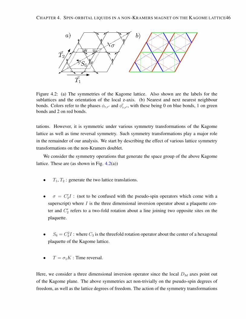
CHAPTER 4. SPIN-ORBITAL LIQUIDS IN A NON-KRAMERS MAGNET ON THE KAGOME LATTICE46
u
v
w
Figure 4.2: (a) The symmetries of the Kagome lattice. Also shown are the labels for thesublattices and the orientation of the local z-axis. (b) Nearest and next nearest neighbourbonds. Colors refer to the phases φr,r′ and φ′r,r′ , with these being 0 on blue bonds, 1 on greenbonds and 2 on red bonds.
tations. However, it is symmetric under various symmetry transformations of the Kagomelattice as well as time reversal symmetry. Such symmetry transformations play a major rolein the remainder of our analysis. We start by describing the effect of various lattice symmetrytransformations on the non-Kramers doublet.
We consider the symmetry operations that generate the space group of the above Kagomelattice. These are (as shown in Fig. 4.2(a))
• T1, T2 : generate the two lattice translations.
• σ = C ′2I : (not to be confused with the pseudo-spin operators which come with asuperscript) where I is the three dimensional inversion operator about a plaquette cen-ter and C ′2 refers to a two-fold rotation about a line joining two opposite sites on theplaquette.
• S6 = C23I : where C3 is the threefold rotation operator about the center of a hexagonal
plaquette of the Kagome lattice.
• T = σ1K : Time reversal.
Here, we consider a three dimensional inversion operator since the local D3d axes point outof the Kagome plane. The above symmetries act non-trivially on the pseudo-spin degrees offreedom, as well as the lattice degrees of freedom. The action of the symmetry transformations

CHAPTER 4. SPIN-ORBITAL LIQUIDS IN A NON-KRAMERS MAGNET ON THE KAGOME LATTICE47
on the pseudo-spin operators is given by,
S6 : σ3, σ+, σ− → σ3, ωσ+, ωσ−,
T : σ3, σ+, σ− → −σ3, σ−, σ+,
C ′2 : σ3, σ+, σ− → −σ3, σ−, σ+,
T1 : σ3, σ+, σ− → σ3, σ+, σ−,
T2 : σ3, σ+, σ− → σ3, σ+, σ−, (4.2)
(ω = ω−1 = ei2π3 ). Operationally their action on the doublet (|+〉 |−〉) can be written in form
of 2× 2 matrices. The translations T1, T2 act trivially on the pseudo-spin degrees of freedom,and the remaining operators act as
T = σ1K, σ = σ1, S6 =
[ω 0
0 ω
], (4.3)
where K refers to complex conjugation. The above expressions can be derived by examiningthe effect of these operators on the wave-function describing the doublet (Eq. 4.1).
We can now write down the most generic pseudo-spin Hamiltonian allowed by the abovelattice symmetries that is bilinear in pseudo-spin operators. The form of the time-reversalsymmetry restricts our attention to those products which are formed by a pair of σ3 operators orthose which mix the pseudo-spin raising and lowering operators. Any term which mixes σ3 andσ± changes sign under the symmetry, and can thus be excluded. Under the C3 transformationabout a site, the terms C3 : σ3
rσ3r′ → σ3
C3(r)σ3C3(r′) and C3 : σ+
r σ−r′ → σ+
C3(r)σ−C3(r′). However,
the term σ+r σ
+r′ (and its Hermitian conjugate) gain additional phase factors when transformed;
under the C3 symmetry transformation, this term becomes C3 : σ+r σ
+r′ → ωσ+
C3(r)σ+C3(r′). In
addition, under the σ symmetry, this term transforms as σ : σ+r σ
+r′ → σ−σ(r)σ
−σ(r′). Thus the
Hamiltonian with spin-spin exchange interactions up to next-nearest neighbour is given by
Heff = Jnn∑〈r,r′〉
[σ3rσ
3r′ + 2(δσ+
r σ−r′ + h.c.) + 2q(e
2πiφr,r′3 σ+
r σ+r′ + h.c.)]
+ Jnnn∑〈〈r,r′〉〉
[σ3rσ
3r′ + 2(δ′σ+
r σ−r′ + h.c.) + 2q′(e
2πiφ′r,r′
3 σ+r σ
+r′ + h.c.)], (4.4)
where φ and φ′ take values 0, 1 and 2 depending on the bonds on which they are defined (Fig.4.2(b)). This takes a similar form to the Hamiltonian derived in Ref. [92], with the coupling δhere allowed to be complex due to the lowered symmetry.

CHAPTER 4. SPIN-ORBITAL LIQUIDS IN A NON-KRAMERS MAGNET ON THE KAGOME LATTICE48
4.3 Spinon representation of the pseudo-spins and PSG anal-ysis
Having written down the pseudo-spin Hamiltonian, we now discuss the possible spin-orbitalliquid phases. We do this in two stages in the following sub-sections.
4.3.1 Slave fermion representation and spinon decoupling
In order to understand these phases, we will use the fermionic slave-particle decompositionof the pseudo-spin operators. At this point, we note that the pseudo-spins satisfy S = 1/2
representations of an “SU(2)” algebra among their generators (not to be confused with theregular spin rotation symmetry). We represent the pseudo-spin degrees of freedom in terms ofa fermion bilinear. This is very similar to usual slave fermion construction for spin liquids[17,18]. We take
σµj =1
2f †jα[ρµ]αβfjβ, (4.5)
where α, β =↑, ↓ is defined along the local z axis and f † (f ) is an S = 1/2 fermionic cre-ation (annihilation) operator. Following standard nomenclature, we refer to the f(f †) as thespinon annihilation (creation) operator, and note that these satisfy standard fermionic anti-commutation relations. The above spinon representation, along with the single occupancyconstraint
f †i↑fi↑ + f †i↓fi↓ = 1, (4.6)
form a faithful representation of the pseudo-spin-1/2 Hilbert space. The above representationof the pseudo-spins, when used in Eq. 4.4, leads to a quartic spinon Hamiltonian. Follow-ing standard procedure,[17, 18] this is then decomposed using auxiliary fields into a quadraticspinon Hamiltonian (after writing down the corresponding Eucledian action). The mean fielddescription of the phases is then characterized by the possible saddle point values of the auxil-iary fields. There are eight such auxiliary fields per bond, corresponding to
χij = 〈f †iαfjα〉∗; ηij = 〈fiα[iτ 2]αβfjβ〉∗; (4.7a)
Eaij = 〈f †iα [τa]αβ fjβ〉
∗; Daij = 〈fiα
[iτ 2τa
]αβfiβ〉∗; (4.7b)
where τa (a = 1, 2, 3) are the Pauli matrices. While Eq. 4.7a represents the usual singletspinon hopping (particle-hole) and pairing (particle-particle) channels, Eq. 4.7b represents thecorresponding triplet decoupling channels. Since the Hamiltonian (Eq. 4.4) does not have

CHAPTER 4. SPIN-ORBITAL LIQUIDS IN A NON-KRAMERS MAGNET ON THE KAGOME LATTICE49
pseudo-spin rotation symmetry, both the singlet and the triplet decouplings are necessary.[20,98]
From this decoupling, we obtain a mean-field Hamiltonian which is quadratic in the spinonoperators. We write this compactly in the following form[20] (subject to the constraint Eq.4.6)
H0 =∑ij
Jij ~f†i Uij
~fj, (4.8)
~f †i =[f †i↑ fi↓ f †i↓ −fi↑
], (4.9)
Uij = ξαβij ΣαΓβ, (4.10)
Σα = ρα ⊗ I; Γβ = I ⊗ τβ, (4.11)
where ρα are the identity (for α = 0) and Pauli matrices (α = 1, 2, 3) acting on pseudo-spindegrees of freedom, and τα represents the same in the gauge space. We immediately note that
[Σα,Γβ
]= 0 ∀α, β. (4.12)
The requirement that H0 be Hermitian restricts the coefficients ξij to satisfy
ξ00ij , ξ
abij ∈ =; ξa0
ij , ξ0bij ∈ <. (4.13)
for a, b ∈ 1, 2, 3. The relations between ξijs and χij, ηij,Eij,Dij are given in Ap-pendix C.[20] As a straight forward extension of the SU(2) gauge theory formulation for spinliquids,[17, 99] we find that H0 is invariant under the gauge transformation
~fj → Wj~fj, (4.14)
Uij → WiUijW†j , (4.15)
where the Wi matrices are SU(2) matrices of the form Wi = ei~Γ·~ai (~Γ ≡ (Γ1,Γ2,Γ3)). Noting
that the physical pseudo-spin operators are given by
~σi =1
4~f †i~Σ~fi, (4.16)
Eq. 4.12 shows that the spin operators, as expected, are gauge invariant. It is useful to definethe “Σ-components” of the Uij matrices as follows:
Uij = VαijΣα, (4.17)

CHAPTER 4. SPIN-ORBITAL LIQUIDS IN A NON-KRAMERS MAGNET ON THE KAGOME LATTICE50
where
Vαij = ξαβij Γβ =
[J αij 0
0 J αij
], (4.18)
and
J αij =
[ξα0ij + ξα3
ij ξα1ij − iξα2
ij
ξα1ij + iξα2
ij ξα0ij − ξα3
ij
]. (4.19)
Under global spin rotations the fermions transform as
~fi → V ~fi, (4.20)
where V is an SU(2) matrix of the form V = ei~Σ·~b (~Σ ≡ Σ1,Σ2,Σ3). So while V0
ij (the singlethopping and pairing) is invariant under spin rotation, V1
ij,V2ij,V3
ij transforms as a vector asexpected since they represent triplet hopping and pairing amplitudes.
4.3.2 PSG Classification
We now classify the non-Kramers spin-orbital liquids based on projective representation simi-lar to that of the conventional quantum spin liquids.[17] Each spin-orbital liquid ground stateof the quadratic Hamiltonian (Eq 4.11) is characterized by the mean field parameters (eighton each bond, χ, η, E1, E2, E3, D2, D2, D3, or equivalently Uij). However, due to the gaugeredundancy of the spinon parametrization (as shown in Eq. 4.15), a general mean-field ansatzneed not be invariant under the symmetry transformations on their own but may be transformedto a gauge equivalent form without breaking the symmetry. Therefore, we must consider itstransformation properties under a projective representation of the symmetry group.[17] Forthis, we need to know the various projective representations of the lattice symmetries of theHamiltonian (Eq. 4.4) in order to classify different spin-orbital liquid states.
Operationally, we need to find different possible sets of gauge transformations GGwhichact in combination with the symmetry transformations SG such that the mean-field ansatzUij is invariant under such a combined transformation. In the case of spin rotation invariantspin-liquids (where only the singlet channels χ and η are present), the above statement isequivalent to demanding the following invariance:
Uij = [GSS]Uij [GSS]† = GS(i)US(i)S(j)G†S(j), (4.21)
where S ∈ SG is a symmetry transformation and GS ∈ GG is the corresponding gauge

CHAPTER 4. SPIN-ORBITAL LIQUIDS IN A NON-KRAMERS MAGNET ON THE KAGOME LATTICE51
transformation. The different possible GS|∀S ∈ SG give the possible algebraic PSGsthat can characterize the different spin-orbital liquid phases. To obtain the different PSGs,we start with various lattice symmetries of the Hamiltonian. The action of various latticetransformations[100] is given by
T1 :(x, y, s)→ (x+ 1, y, s);
T2 :(x, y, s)→ (x, y + 1, s);
σ :(x, y, u)→ (y, x, u);
(x, y, v)→ (y, x, w);
(x, y, w)→ (y, x, v);
S6 :(x, y, u)→ (−y − 1, x+ y + 1, v);
(x, y, v)→ (−y, x+ y, w);
(x, y, w)→ (−y − 1, x+ y, u); (4.22)
where (x, y) denotes the lattice coordinates and s ∈ u, v, w denotes the sub-lattice index(see figure 4.2).
In terms of the symmetries of the Kagome lattice, these operators obey the following con-ditions
T 2 = σ2 = (S6)6 = e,
g−1T−1gT = e ∀g ∈ SG,
T−12 T−1
1 T2T1 = e,
σ−1T−11 σT2 = e,
σ−1T−12 σT1 = e,
S−16 T−1
2 S6T1 = e,
S−16 T−1
2 T1S6T2 = e,
σ−1S6σS6 = e. (4.23)
In addition, these commutation relations are valid in terms of the operations on the pseudo-spindegrees of freedom, as can be verified from Eq. 4.3.
In addition to the conditions in Eq. 4.23, the Hamiltonian is trivially invariant under theidentity transformation. The invariant gauge group (IGG) of an ansatz is defined as the setof all pure gauge transformations GI such that GI : Uij → Uij . The nature of such puregauge transformations immediately dictates the nature of the low energy fluctuations about the

CHAPTER 4. SPIN-ORBITAL LIQUIDS IN A NON-KRAMERS MAGNET ON THE KAGOME LATTICE52
mean field state. If these fluctuations do not destabilize the mean-field state, we get stable spinliquid phases whose low energy properties are controlled by the IGG. Accordingly, spin liq-uids obtained within projective classification are primarily labelled by their IGGs and we haveZ2, U(1) and SU(2) spin liquids corresponding to IGGs of Z2, U(1) and SU(2) respectively.In this section we concentrate on the set of Z2 “spin liquids” (spin-orbital liquids with a Z2
IGG).
We now focus on the PSG classification. As shown in Eq. 4.2, in the present case, thepseudo-spins transform non-trivially under different lattice symmetry transformations. Dueto the presence of the triplet decoupling channels the non-Kramers doublet transforms non-trivially under lattice symmetries (Eq. 4.3). Thus, the invariance condition on the Uijs is notgiven by Eq. 4.21, but by a more general condition
Uij = [GSS]Uij [GSS]† = GS(i)φS[US(i)S(j)
]G†S(j). (4.24)
Here
φS[US(i)S(j)
]= DSUS(i)S(j)D†S, (4.25)
andDS generates the pseudo-spin rotation associated with the symmetry transformation (S) onthe doublet. The matrices DS have the form
DS6 = −1
2Σ0 − i
√3
2Σ3, (4.26)
Dσ = DT = i ∗ Σ1, DT1 = DT2 = Σ0. (4.27)
Under these constraints, we must determine the relations between the gauge transformationmatrices GS(i) for our set of ansatz. The additional spin transformation (Eq. 4.25) does not af-fect the structure of the gauge transformations, as the gauge and spin portions of our ansatz arenaturally separate (Eq. 4.12). In particular, we can choose to define our gauge transformationssuch that
GS : Uij = GS : ξαβij ΣαΓβ → ξαβij ΣαG†S(i)ΓβGS(j), (4.28)
S : Uij = S : ξαβij ΣαΓβ → ξαβS(i)S(j)DSΣαD†SΓβ, (4.29)
where we have used the notation GS : Uij ≡ G†S(i)UijGS(j) and so forth. As a result, we canbuild on the general construction of Lu et al.[100] to derive the form of the gauge transforma-tion matrices. The details are given in Appendix B.1.
For a particular example of this construction, we consider the commutation relation be-

CHAPTER 4. SPIN-ORBITAL LIQUIDS IN A NON-KRAMERS MAGNET ON THE KAGOME LATTICE53
tween the translation operators, T−12 T−1
1 T2T1 = I . Acting these operations on the ansatz inturn, combined with their gauge transformations, we can see that T−1
2 G†T2T−11 G†T1GT2T2GT1T1
must act trivially on the ansatz (or leave the ansatz invariant). Hence, the gauge transformationportion of this must belong to the IGG, i.e.
G†T2(T−11 (i))G†T1(i)GT2(i)GT1(T
−12 (i)) = W ′
i , (4.30)
where W ′i is an IGG transformation. We can also see that under a gauge transformation Wi
the transformations GS transform according to GS(i) → WiGS(i)W †S−1(i). We can therefore
determine groups of equivalent GS’s which can be connected by gauge transformations, anduse this to distinguish different quantum states.
Considering Z2 spin liquids, the gauge transformations defined above must therefore satisfyW ′i = η12I , where I is the identity matrix and η12 = ±1. Ansatze which satisfy η12 = +1 and
η12 = −1 cannot be continuously connected to one another. These Z2 variables thus distinguishdifferent quantum phases. By solving these equations for each relation between the symmetryoperations, i.e. all of the relations in a presentation of the space group, we can categorize thepossible quantum phases to which an ansatz can belong.
A major difference arises when examining the set of algebraic PSGs for Z2 spin liquidsfound on the Kagome lattice due to the difference between the structure of the time reversalsymmetry operation on the Kramers and non-Kramers pseudo-spin-1/2s. In the present case,we find there are 30 invariant PSGs leading to thirty possible spin-orbital liquids. This is incontrast with the Kramers case analysed by Lu et al.,[100] where ten of the algebraic PSGscannot be realized as invariant PSGs, as all bonds in these ansatz are predicted to vanish iden-tically due to the form of the time reversal operator, and hence there are only twenty possiblespin liquids. However, with the inclusion of spin triplet terms and the non-Kramers form ofour time reversal operator, these ansatz are now realizable as invariant PSGs as well. The timereversal operator, as defined in Appendix B.1, acts as
T : ξαβij ΣαΓβ → ξαβij ΣαΓβ, (4.31)
where ξαβ = ξαβ if α ∈ 1, 2 and ξαβ = −ξαβ if α ∈ 0, 3. The projective implementationof the time-reversal symmetry condition (Eq. 4.23) takes the form (see Appendix B.1)
[GT (i)]2 = ηT I ∀i, (4.32)
where GT (i) is the gauge transformation associated with time reversal operation and ηT = ±1
for a Z2 IGG.

CHAPTER 4. SPIN-ORBITAL LIQUIDS IN A NON-KRAMERS MAGNET ON THE KAGOME LATTICE54
Therefore, the terms allowed by the time reversal symmetry to be non zero are, for ηT = 1,
ξ10, ξ11, ξ12, ξ13, ξ20, ξ21, ξ22, ξ23, (4.33)
and for ηT = −1, with the choice GT (i) = iΓ1 (see appendix B.1),
ξ02, ξ03, ξ10, ξ11, ξ20, ξ21, ξ32, ξ33. (4.34)
This contrasts with the case of Kramers doublets, in which no terms are allowed for ηT = −1,and for ηT = −1 the allowed terms are
ξ02, ξ03, ξ12, ξ13, ξ22, ξ23, ξ32, ξ33. (4.35)
Further restrictions on the allowed terms on each link arise from the form of the gaugetransformations defined for the symmetry transformations. All nearest neighbour bonds canthen be generated from Uij defined on a single bond, by performing appropriate symmetryoperations.
Using the methods outlined in earlier works (Ref. [17], [100]) we find the minimum set ofparameters required to stabilizeZ2 spin-orbital liquids. We take into consideration up to secondneighbour hopping and pairing amplitudes (both singlet and triplet channels). The results arelisted in Table 4.1.
The spin-orbital liquids listed from 21−30 are not allowed in the case of Kramers doubletsand, as pointed out before, their existence is solely due to the unusual action of the time-reversal symmetry operator on the non-Kramers spins. Hence these ten spin-orbital liquidsare qualitatively new phases that may appear in these systems. Of these ten phases, only two
(labelled as 21 and 22 in Table 4.1) require next nearest neighbour amplitudes to obtain a Z2
spin-orbital liquid. For the other eight, nearest neighbour amplitudes are already sufficient tostabilize a Z2 spin-orbital liquid.
It is interesting to note (see below) that bond-pseudo-spin-nematic order (Eq. 4.36 andEq. 4.37) can signal spontaneous time-reversal symmetry breaking. Generally, since the tripletdecouplings are present, the bond nematic order parameter for the pseudo-spins[45, 101]
Qαβij = 〈(Sαi S
βj + Sβi S
αj
)/2− δαβ(~Si · ~Sj)/3〉, (4.36)
as well as vector chirality order
~Jij = 〈~Si × ~Sj〉, (4.37)
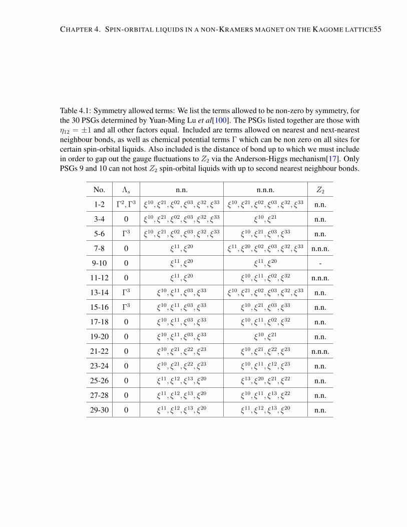
CHAPTER 4. SPIN-ORBITAL LIQUIDS IN A NON-KRAMERS MAGNET ON THE KAGOME LATTICE55
Table 4.1: Symmetry allowed terms: We list the terms allowed to be non-zero by symmetry, forthe 30 PSGs determined by Yuan-Ming Lu et al[100]. The PSGs listed together are those withη12 = ±1 and all other factors equal. Included are terms allowed on nearest and next-nearestneighbour bonds, as well as chemical potential terms Γ which can be non zero on all sites forcertain spin-orbital liquids. Also included is the distance of bond up to which we must includein order to gap out the gauge fluctuations to Z2 via the Anderson-Higgs mechanism[17]. OnlyPSGs 9 and 10 can not host Z2 spin-orbital liquids with up to second nearest neighbour bonds.
No. Λs n.n. n.n.n. Z2
1-2 Γ2,Γ3 ξ10, ξ21, ξ02, ξ03, ξ32, ξ33 ξ10, ξ21, ξ02, ξ03, ξ32, ξ33 n.n.
3-4 0 ξ10, ξ21, ξ02, ξ03, ξ32, ξ33 ξ10, ξ21 n.n.
5-6 Γ3 ξ10, ξ21, ξ02, ξ03, ξ32, ξ33 ξ10, ξ21, ξ03, ξ33 n.n.
7-8 0 ξ11, ξ20 ξ11, ξ20, ξ02, ξ03, ξ32, ξ33 n.n.n.
9-10 0 ξ11, ξ20 ξ11, ξ20 -
11-12 0 ξ11, ξ20 ξ10, ξ11, ξ02, ξ32 n.n.n.
13-14 Γ3 ξ10, ξ11, ξ03, ξ33 ξ10, ξ21, ξ02, ξ03, ξ32, ξ33 n.n.
15-16 Γ3 ξ10, ξ11, ξ03, ξ33 ξ10, ξ21, ξ03, ξ33 n.n.
17-18 0 ξ10, ξ11, ξ03, ξ33 ξ10, ξ11, ξ02, ξ32 n.n.
19-20 0 ξ10, ξ11, ξ03, ξ33 ξ10, ξ21 n.n.
21-22 0 ξ10, ξ21, ξ22, ξ23 ξ10, ξ21, ξ22, ξ23 n.n.n.
23-24 0 ξ10, ξ21, ξ22, ξ23 ξ10, ξ11, ξ12, ξ23 n.n.
25-26 0 ξ11, ξ12, ξ13, ξ20 ξ13, ξ20, ξ21, ξ22 n.n.
27-28 0 ξ11, ξ12, ξ13, ξ20 ξ10, ξ11, ξ13, ξ22 n.n.
29-30 0 ξ11, ξ12, ξ13, ξ20 ξ11, ξ12, ξ13, ξ20 n.n.

CHAPTER 4. SPIN-ORBITAL LIQUIDS IN A NON-KRAMERS MAGNET ON THE KAGOME LATTICE56
are non zero. Since the underlying Hamiltonian Eq. 4.4) generally does not have pseudo-spin rotation symmetry, the above non-zero expectation values do not spontaneously breakany pseudo-spin rotation symmetry. However, because of the unusual transformation prop-erty of the non-Kramers pseudo-spins under time reversal, the operators corresponding toQ13ij ,Q23
ij ,J 1ij,J 2
ij are odd under time reversal, a symmetry of the pseudo-spin Hamiltonian.Hence if any of the above operators gain a non-zero expectation value in the ground state,then the corresponding spin-orbital liquid breaks time reversal symmetry. While this can occurin principle, we check explicitly (see Appendix C) that in all the spin-orbital liquids discussedabove, the expectation values of these operators are identically zero. This provides a non-trivialconsistency check on our PSG calculations.
Having identified the possible Z2 spin-orbital liquids, we can now study typical dynamicstructure factors for these spin-orbital liquids. In the next section we examine the typicalspinon band structure for different spin-orbital liquids obtained above and find their dynamicspin structure factor.
4.4 Dynamic Spin Structure Factor
We compute the dynamic spin structure factor
S(q, ω) =
∫dt
2πeiωt
∑ij
eiq·(ri−rj)∑
a=1,2,3
〈σai (t)σaj (0)〉, (4.38)
for two example ansatz of our spin liquid candidates, in order to demonstrate the qualitative dif-ferences between the Kramers and non-Kramers spin-orbital liquids. In the above equation, thepseudo-spin variables are defined in a global basis (with the z-axis perpendicular to the Kagomeplane). In computing the structure factor for the non-Kramers example, we include only the σ3
components of the pseudo-spin operator in the local basis, since only the z-components carrymagnetic dipole moment (see discussion before). Hence, only this component couples linearlyto neutrons in a neutron scattering experiment.
Eq. 4.38 fails to be periodic in the first Brillouin zone of the Kagome lattice[98], as the termri− rj in eq. 4.38 is a half-integer multiple of the primitive lattice vectors when the sublatticesof sites i and j are not equal. As such, we examine the structure factor in the extended Brillouinzone, which consists of those momenta of length up to double that of those in the first Brillouinzone. We plot the structure factor along the cut Γ→ M ′ → K ′ → Γ, where M ′ = 2M and K ′
= 2K. We examine the structure factors for two ansatz of spin liquids # 17 and # 3, which havebeen studied in the case of Kramers spin liquids [98] and have non-Kramers analogues.
As expected, we find that the structure factor has greater weight in the case of a Kramers

CHAPTER 4. SPIN-ORBITAL LIQUIDS IN A NON-KRAMERS MAGNET ON THE KAGOME LATTICE57
ω S(q,ω)
q
Figure 4.3: The spin structure factor for an ansatz in spin liquid 17, with the spin variablestransforming as a Kramers doublet. The energy scale, ω, is determined by the spinon band-width, and the intensity is in arbitrary units (shared by figures 4.4, 4.5 and 4.6).
ω S(q,ω)
q
Figure 4.4: The spin structure factor for an ansatz in spin liquid 17, with the spin variablestransforming as a non-Kramers doublet.
ω S(q,ω)
q
Figure 4.5: The spin structure factor for an ansatz in spin liquid 5, with the spin variablestransforming as a Kramers doublet.

CHAPTER 4. SPIN-ORBITAL LIQUIDS IN A NON-KRAMERS MAGNET ON THE KAGOME LATTICE58
ω S(q,ω)
q
Figure 4.6: The spin structure factor for an ansatz in spin liquid 5, with the spin variablestransforming as a non-Kramers doublet.
spin liquid. This is partially due to the fact that the moment of the scattering particle coupleswith all components of the spin, rather than simply the z-component. In addition, we notethat the presence of different mean field parameters associated with non-Kramers spin-orbitalliquids can drive the formation or elimination of a spinon gap. Qualitative and quantitative dif-ferences such as these, which can be observed in these structure factors between Kramers andnon-Kramers spin-orbital liquids, provides one possible distinguishing experimental signatureof these states. We shall not pursue this in detail in the present section.
We now briefly dicuss the effect of the fluctuations about the mean-field states. In the ab-sence of pairing channels (both singlet and triplet) the gauge group is U(1). In this case, thefluctuations of the gauge field about the mean field (Eq. 4.15) are related to the scalar pseudo-spin chirality ~S1 · ~S2 × ~S3, where the three sites form a triangle.[102] Such fluctuations aregapless in a U(1) spin liquid. It is interesting to note that the scalar spin-chirality is odd undertime-reversal symmetry and it has been proposed that such fluctuations can be detected in neu-tron scattering experiments in presence of spin rotation symmetry breaking.[103] In the presentcase, however, due to the presence of spinon pairing, the gauge group is broken down to Z2 andthe above gauge fluctuations are rendered gapped through Anderson-Higg’s mechanism.[17]
In addition to the above gauge fluctuations, because of the triplet decouplings which breakpseudo-spin rotational symmetry, there are bond quadrupolar fluctuations of the pseudo-spinsQαβij (Eq. 4.36), as well as vector chirality fluctuations ~Jij (Eq. 4.37)[45, 101] on the bonds.These nematic and vector chirality fluctuations are gapped because the underlying pseudo-spinHamiltonian (Eq. 4.4) breaks pseudo-spin-rotation symmetry. However, we note that becauseof the unusual transformation of the non-Kramers pseudo-spins under time reversal (only thez−component of pseudo-spins being odd under time reversal), Q13
ij ,Q23ij ,J 1
ij and J 2ij are odd
under time reversal. Hence, while their mean field expectation values are zero (see above), the

CHAPTER 4. SPIN-ORBITAL LIQUIDS IN A NON-KRAMERS MAGNET ON THE KAGOME LATTICE59
fluctuations of these quantities can in principle linearly couple to the neutrons in addition tothe z−component of the pseudo-spins.
4.5 Discussion and possible experimental signature of non-Kramers spin-orbital liquids
In this chapter, we have outlined the possible Z2 spin-orbital liquids, with gapped or gaplessfermionic spinons, that can be obtained in a system of non-Kramers pseudo-spin-1/2s on aKagome lattice of Pr+3 ions. We find a total of thirty, 10 more than in the case of correspond-ing Kramers system, allowed within PSG analysis in the presence of time reversal symmetry.The larger number of spin-orbital liquids is a result of the difference in the action of the time-reversal operator, when realized projectively. We note that the spin-spin dynamic structurefactor can bear important signatures of a non-Kramers spin-orbital liquid when compared totheir Kramers counterparts. Our analysis of the number of invariant PSGs leading to possi-bly different spin-orbital liquids that may be realizable in other lattice geometries will forminteresting future directions.
We now briefly discuss an experiment that can play an important role in determining non-Kramers spin-orbital liquids. Since the non-Kramers doublets are protected by crystalline sym-metries, lattice strains can linearly couple to the pseudo-spins. As we discussed, the transverse(x and y) components of the pseudo-spins σ1, σ2 carry quadrupolar moments and hence areeven under the time reversal transformation. Further, they transform under an Eg irreduciblerepresentation of the local D3d crystal field. Hence any lattice strain which has this symmetrycan linearly couple to the above two transverse components. It turns out that in the crystal typeof which we are concerned, there is indeed such a mode related to the distortion of the oxygenoctahedra. Symmetry considerations show that the linear coupling is of the formEg1σ
1+Eg2σ2
(Eg1, Eg2 being the two components of the distortion in the local basis). The above modeis Raman active. For a spin-liquid, we expect that as the temperature is lowered, the spinonsbecome more prominent as deconfined quasiparticles. So the Raman active phonon can effi-ciently decay into the spinons due to the above coupling channel. If the spin liquid is gapless,then this will lead to anomalous broadening of the above Raman mode as the temperature islowered, which, if observed, can be an experimental signature of the non-Kramers spin-orbitalliquid. The above coupling is forbidden in Kramers doublets by time-reversal symmetry andhence no such anomalous broadening is expected.

Chapter 5
Quantum Spin Liquid in a BreathingKagome Lattice
5.1 Introduction
The kagome antiferromagnet is of interest both experimentally and theoretically, with numeri-cal studies[104, 105, 106, 107, 108, 109, 110] suggesting a spin liquid[111, 112, 113, 114, 115]as the ground state of the Heisenberg model, and the material Herbertsmithite believed to re-alise spin liquid physics at low temperatures.[9, 98, 116, 117, 118, 119, 120, 121, 122, 123,124]
Recent experiments on a vanadium based material [NH4]2[C7H14N][V7O6F18] (diammo-nium quinuclidinium vanadium oxyfluoride; DQVOF) have suggested the possibility that thissystem exhibits spin liquid behaviour.[13, 14] This material contains two-dimensional struc-tures, consisting of three planes of vanadium ions (along with non-magnetic oxygen and fluo-rine ions) which are separated from other three-plane structures by non-magnetic atoms. Thesethree planes consist of two kagome lattice planes of spin-1/2 V4+ ions separated by one layerof spin-1 V3+ ions arranged in a triangular lattice. The kagome lattices appear to have verylittle disorder and to be formed of equilateral triangles, which, along with the small spin-orbitcoupling present for 3d atoms, suggests that the highly frustrated Heisenberg model may be agood approximation of the spin physics in these layers. However, the up and down trianglesdiffer in size, requiring an anisotropic Heisenberg model to describe the physics of this breath-ing kagome lattice. These kagome layers appear to be well isolated from one another and tocouple only weakly to the intermediate triangular lattice layers, offering a possible realisationof a nearly isolated kagome lattice antiferromagnet without disorder.
Motivated by this discovery, we study the anisotropic Heisenberg model on the kagome
60

CHAPTER 5. QUANTUM SPIN LIQUID IN A BREATHING KAGOME LATTICE 61
V2
O
FV1
Figure 5.1: The local structure of the compound DQVOF.[13] The upper and lower trianglesof spin-1/2 vanadium (V1) ions form parts of separate breathing kagome lattices, which areconnected by layers of spin-1 vanadium (V2) ions.
Figure 5.2: The breathing kagome lattice in DQVOF. Each downwards facing triangle has thelocal structure shown in figure 5.1.

CHAPTER 5. QUANTUM SPIN LIQUID IN A BREATHING KAGOME LATTICE 62
lattice. Classically, this model is as frustrated as the fully isotropic Heisenberg model, withthe ground state manifold being those states for which the sum of the classical spin vectors oneach triangle is zero. However, the full quantum model may show substantial differences. Theisotropic model has been studied using a number of methods, including variational Monte Carlo(VMC)[108, 109, 110] and density matrix renormalization group (DMRG)[104, 105, 106, 107]numerical studies. The earlier VMC calculations indicated that a gapless U(1) spin liquidwith a Dirac spinon excitation was the ground state.[108, 109] However, a more recent VMCcalculation challenges this claim, finding instead that a gapped Z2 spin liquid has the lowerenergy.[110] DMRG studies find a gapped spin liquid ground state for the nearest neighbourHeisenberg model.[105, 106] When a next nearest neighbour Heisenberg interaction is added,the entanglement entropy can be calculated, which suggests a Z2 spin liquid ground state.[107]However, the nearest neighbour limit is more subtle, with the numerical computations havingdifficulty unambiguously determining the nature of the ground state. This may be due to thepresence of many energetically competing spin liquid states, or to the proximity to a quantumcritical point. Hence, a perturbative deformation of the isotropic nearest neighbour model mayserve to stabilize a unique spin liquid ground state. The breathing kagome lattice offers suchan opportunity, which may lead to a better comparison between theoretical predictions andexperimental results.
In this work, we investigate the quantum spin liquid ground state of the breathing kagomelattice. In particular, we show that the VMC in the fermion basis clearly favors a gappedZ2 spin liquid. We narrow our search to consider only those phases which respect all of thesymmetries of the Hamiltonian, as has been shown to be reliable for the isotropic kagome latticeHeisenberg model.[110] In order to systematically study these phases, we first classify thepossible spin liquid phases, using the projective symmetry group (PSG) analysis of symmetricspin liquids.[125] We make a clear connection between the results of our analysis and theisotropic kagome lattice results.[112, 115] We also derive the connection between the bosonicand fermionic spin liquids, by considering the PSG of the vison excitations.[126, 127]
The remainder of the paper is organized as follows. In section 5.2, we describe the detailsof the model, along with the symmetries present on this lattice. Next, we examine the possiblesymmetric spin liquid phases in this model using the PSG formalism. In section 5.3, we con-sider the fermionic mean field states, and in section 5.4 we consider the bosonic states. We alsoexamine the relation between the two types of spin liquids in section 5.5. In addition to this, wecomment on the relation between the isotropic kagome lattice and anisotropic kagome latticesolutions found, and show that each of the anisotropic kagome lattice solutions connects to cer-tain isotropic lattice solutions.[112, 115] Each isotropic lattice solution can also be consideredas a special case of the anisotropic lattice solutions, as one would expect, fully describing the
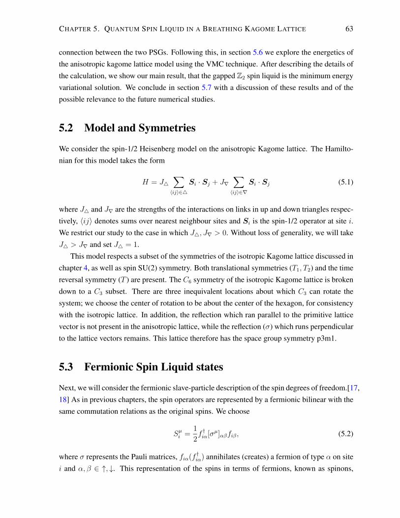
CHAPTER 5. QUANTUM SPIN LIQUID IN A BREATHING KAGOME LATTICE 63
connection between the two PSGs. Following this, in section 5.6 we explore the energetics ofthe anisotropic kagome lattice model using the VMC technique. After describing the details ofthe calculation, we show our main result, that the gapped Z2 spin liquid is the minimum energyvariational solution. We conclude in section 5.7 with a discussion of these results and of thepossible relevance to the future numerical studies.
5.2 Model and Symmetries
We consider the spin-1/2 Heisenberg model on the anisotropic Kagome lattice. The Hamilto-nian for this model takes the form
H = J4∑〈ij〉∈4
Si · Sj + J∇∑〈ij〉∈∇
Si · Sj (5.1)
where J4 and J∇ are the strengths of the interactions on links in up and down triangles respec-tively, 〈ij〉 denotes sums over nearest neighbour sites and Si is the spin-1/2 operator at site i.We restrict our study to the case in which J4, J∇ > 0. Without loss of generality, we will takeJ4 > J∇ and set J4 = 1.
This model respects a subset of the symmetries of the isotropic Kagome lattice discussed inchapter 4, as well as spin SU(2) symmetry. Both translational symmetries (T1, T2) and the timereversal symmetry (T ) are present. The C6 symmetry of the isotropic Kagome lattice is brokendown to a C3 subset. There are three inequivalent locations about which C3 can rotate thesystem; we choose the center of rotation to be about the center of the hexagon, for consistencywith the isotropic lattice. In addition, the reflection which ran parallel to the primitive latticevector is not present in the anisotropic lattice, while the reflection (σ) which runs perpendicularto the lattice vectors remains. This lattice therefore has the space group symmetry p3m1.
5.3 Fermionic Spin Liquid states
Next, we will consider the fermionic slave-particle description of the spin degrees of freedom.[17,18] As in previous chapters, the spin operators are represented by a fermionic bilinear with thesame commutation relations as the original spins. We choose
Sµi =1
2f †iα[σµ]αβfiβ, (5.2)
where σ represents the Pauli matrices, fiα(f †iα) annihilates (creates) a fermion of type α on sitei and α, β ∈ ↑, ↓. This representation of the spins in terms of fermions, known as spinons,

CHAPTER 5. QUANTUM SPIN LIQUID IN A BREATHING KAGOME LATTICE 64
Figure 5.3: The anisotropic (breathing) kagome lattice. Outlined is a single unit cell, consist-ing of three lattice sites. Also shown are the four symmetry operations required to generatethe space group. The size difference between the inequivalent triangles has been exaggeratedcompared to experiment, for clarity of presentation.[13]
along with the single fermion per site constraint
f †i↑fi↑ + f †i↓fi↓ = 1, (5.3)
gives a faithful representation of the Hilbert space. At this point, the analysis is exact (i.e.no approximations have been made) and the spin Hamiltonian appears as a quartic spinonHamiltonian. Using a mean-field decoupling we can decompose this Hamiltonian in terms ofauxiliary fields, leading to a quadratic Hamiltonian in terms of the fermionic spinons.
Unlike in previous chapters, the Hamiltonian of the spin liquid which we wish to considerhere has an SU(2) spin symmetry. To describe such a spin liquid, we choose a decomposi-tion in which only the singlet spinon hopping and pairing channels appear in the mean fieldHamiltonian. These take the form
χij = 〈f †iαfjα〉, ∆ij = 〈fiα[iτ 2]αβfjβ〉, (5.4)
where τ represents Pauli matrices. This decomposition leads to a mean field Hamiltonian ofthe form
H0 =∑ij
Jij ~fi†Uij ~fj +
∑i
3∑l=1
Λl ~fi†τ l ~fi
Uij =
[χ†ij ∆ij
∆†ij −χij
], ~fi =
[fi↑
f †i↓
]. (5.5)
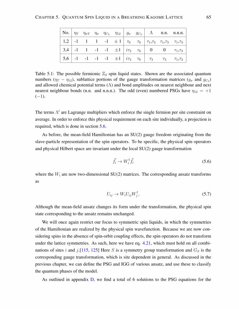
CHAPTER 5. QUANTUM SPIN LIQUID IN A BREATHING KAGOME LATTICE 65
No. ηT ησT ησ ηC3 η12 gσ gC3 Λ n.n. n.n.n.
1,2 -1 1 1 -1 ± 1 τ0 τ0 τ1,τ3 τ1,τ3 τ1,τ3
3,4 -1 1 -1 -1 ±1 iτ2 τ0 0 0 τ1,τ3
5,6 -1 -1 -1 -1 ±1 iτ3 τ0 τ3 τ3 τ1,τ3
Table 5.1: The possible fermionic Z2 spin liquid states. Shown are the associated quantumnumbers (ηT − η12), sublattice portions of the gauge transformation matrices (gσ and gC3)and allowed chemical potential terms (Λ) and bond amplitudes on nearest neighbour and nextnearest neighbour bonds (n.n. and n.n.n.). The odd (even) numbered PSGs have η12 = +1(−1).
The terms Λl are Lagrange multipliers which enforce the single fermion per site constraint onaverage. In order to enforce this physical requirement on each site individually, a projection isrequired, which is done in section 5.6.
As before, the mean-field Hamiltonian has an SU(2) gauge freedom originating from theslave-particle representation of the spin operators. To be specific, the physical spin operatorsand physical Hilbert space are invariant under the local SU(2) gauge transformation
~fi → W †i~fi (5.6)
where the Wi are now two-dimensional SU(2) matrices. The corresponding ansatz transformsas
Uij → WiUijW†j , (5.7)
Although the mean-field ansatz changes its form under the transformation, the physical spinstate corresponding to the ansatz remains unchanged.
We will once again restrict our focus to symmetric spin liquids, in which the symmetriesof the Hamiltonian are realized by the physical spin wavefunction. Because we are now con-sidering spins in the absence of spin-orbit coupling effects, the spin operators do not transformunder the lattice symmetries. As such, here we have eq. 4.21, which must hold on all combi-nations of sites i and j.[115, 125] Here S is a symmetry group transformation and GS is thecorresponding gauge transformation, which is site dependent in general. As discussed in theprevious chapter, we can define the PSG and IGG of various ansatz, and use these to classifythe quantum phases of the model.
As outlined in appendix D, we find a total of 6 solutions to the PSG equations for the

CHAPTER 5. QUANTUM SPIN LIQUID IN A BREATHING KAGOME LATTICE 66
anisotropic kagome lattice which allow non-zero amplitudes for the Uij . The form of thesesolutions are detailed in table 5.1. The full gauge transformation matrices take the form
GT1(x, y, s) = ηy12I, (5.8)
GT2(x, y, s) = I, (5.9)
Gσ(x, y, s) = ηxy12 gσ, (5.10)
GC3(x, y, s) = −ηy(y+1)/2+xy12 I, (5.11)
where the position (x, y, s) is represented by using the coordinate system in Fig. 5.3 and thesublattice index s. In this expression, gσ ≡ Gσ(0, 0, s) can be chosen to be identical on eachsublattice, and GC3 is proportional to the identity matrix.
We have found 6 possible PSGs for the anistotropic kagome lattice, compared to 20 for theisotropic version of this lattice (Ref. [115]). In order to reconcile this result, we note that, onthe anisotropic kagome lattice, up and down triangles are no longer related by symmetry. Asa result, we have additional mean field parameters corresponding to these inequivalent bonds.Although we have fewer PSGs, we can realize all 20 of the isotropic kagome lattice PSGs asspecial cases of the 6 anisotropic kagome lattice PSGs.
The simplest way to see this is to consider the product of the gauge transformations asso-ciated with the symmetry transformations. Following the work of Lu et. al. in Ref. [115], andconsidering that C3 is C2
6 , in terms of the gauge transformations the solution for the isotropickagome lattice case can be seen as a special point in the solution set for the anisotropic kagomelattice if GC3(i) = GC6(i)GC6(C
−16 (i)) for all i, up to gauge transformations. This is the case
due to the fact that in the isotropic case we have
Uij = GC6(i)UC−16 (i),C−1
6 (j)G†C6
(j)
= GC6(i)GC6(C−16 (i))UC−1
3 (i),C−13 (j)G
†C6
(C−16 (j))G†C6
(j), (5.12)
and thus for these to match, GC6(i)GC6(C−16 (i)) must be gauge equivalent to GC3(i). When
this occurs, the isotropic kagome lattice PSG can be continuously connected to the anisotropickagome lattice PSG.
Applying this to the spin liquids on the isotropic kagome lattice, we determine the corre-spondence between the isotropic kagome lattice states and those on the anisotropic kagomelattice. It can be seen that all of the PSGs for the anisotropic kagome lattice have specialpoints which correspond to isotropic kagome lattice PSGs. This must be determined explicitly;anisotropic lattice PSGs 1-4 each correspond to three isotropic lattice PSGs, while PSGs 5 and6 each correspond to four isotropic lattice PSGs. The isotropic lattice PSGs which share the

CHAPTER 5. QUANTUM SPIN LIQUID IN A BREATHING KAGOME LATTICE 67
values of η12 and Gσ all belong to the same anisotropic lattice PSG, regardless of their valuesof GC6 .
As is noted in table 5.1, only PSGs 3 and 4 do not allow any amplitude for mean fieldparameters on nearest neighbour bonds, nor do they support chemical potential terms. In thiscase, only two free parameters appear up to second neighbour terms. For PSGs 5 and 6, nearestneighbour pairing and pairing chemical potential terms are disallowed, and second neighbourhopping and pairing are required to stabilize a Z2 spin liquid state. In PSGs 1 and 2, bothnearest neighbour hopping and pairing are allowed, as well as two on site chemical potentialterms and second neighbour hopping and pairing.
Of particular note for our considerations is PSG 2, which contains the Z2[0, π]β phase ofthe isotropic kagome lattice[115] in the limit that the nearest neighbour hopping and pairingamplitudes are equal on the up and down triangles. On the anisotropic kagome lattice, wecan remove one of the pairing parameters using a gauge transformation; here we choose toremove the nearest neighbour pairing on one of the triangles, ∆4. The corresponding meanfield Hamiltonian takes the form
HMF =∑i
[µ∑α
f †i,αfi,α + η(fi,↑fi,↓ +H.c.)
]+ χ4
∑〈i,j〉∈4,α
f †i,αfj,α
+∑〈i,j〉∈∇
si,j
[χ∇∑α
f †i,αfj,α + ∆∇(fi,↑fj,↓ +H.c.)
]
+∑〈〈i,j〉〉
νi,j
[χ2
∑α
f †i,αfj,α + ∆2(fi,↑fj,↓ +H.c.)
], (5.13)
up to second neighbour terms, where µ and η are the chemical potential terms, χ4,∇,2 arehopping terms on up-triangle nearest neighbour bonds, down-triangle nearest neighbour bondsand second neighbour bonds, ∆∇,2 are pairing terms on down-triangle nearest neighbour bondsand second neighbour bonds, and sij and νij take values of ±1, fixed by a gauge choice.
5.4 Bosonic Spin Liquid states
We also consider the form of the bosonic spin liquid states which can appear on the anisotropickagome lattice.[111, 112] The analysis proceeds in a similar fashion to the fermionic case,where we now choose
Sµi =1
2b†iα[σµ]αβbjβ, (5.14)

CHAPTER 5. QUANTUM SPIN LIQUID IN A BREATHING KAGOME LATTICE 68
Figure 5.4: The sign structure of the different bonds in PSG 2. Coloured is the extendedunit cell which repeats over the lattice, with blue and red bonds representing sij = +1 andsij = −1 respectively on the down triangles. Also shown with dotted lines are the secondneighbour bonds, with the same sign structure for νij as above.
where σ again represents the Pauli matrices, biα(b†iα) now annihilates (creates) a boson of typeα on site i and α, β ∈ ↑, ↓. The constraint on the number of spinons appearing on each sitetakes a different form between the two theories; in the Schwinger boson theory, we take thatconstraint to be
b†i↑bi↑ + b†i↓bi↓ = κ, (5.15)
where κ = 2S for the physical wavefunction of a spin system with spin S. In the mean-fieldtheory, κ is often taken to be a continuous positive real parameter.
Following Ref. [112], we note that the spin bilinears appearing in the Heisenberg Hamilto-nian take the form
~Si · ~Sj =: B†ijBij : −A†ijAij, (5.16)
where the boson hopping and pairing operators Bij and Aij are of the form
Bij =1
2(b†i↑bj↑ + b†i↓bj↓), Aij =
1
2(bi↑bj↓ − bi↓bj↑). (5.17)
This suggests a natural mean field Hamiltonian for the bosonic spinons, taking the form
H0 =∑ij
Jij(−A∗ijAij +B∗ijBij + h.c.)− µ∑i
(∑σ
b†iσbiσ − κ), (5.18)
with Aij , Bij and µ parameters which determine the form of the mean field wavefunction.Here, we have ignored constants which do not affect the form of the wavefunction for a givenparameter set. Similar to the case of fermionic spinons, this Hamiltonian is invariant undera local gauge transformation which leaves the physical spin operators invariant; however, thegauge group of the transformations for bosons is U(1), rather than the SU(2) transformations

CHAPTER 5. QUANTUM SPIN LIQUID IN A BREATHING KAGOME LATTICE 69
for fermions. Under a gauge transformation, the bosons gain a phase factor
bi,σ → eiφibi,σ (5.19)
and the mean field parameters transform as
Aij → ei(−φi−φj)Aij, Bij → ei(φi−φj)Bij. (5.20)
We can classify the possible bosonic spin liquid states which appear on this lattice in thesame manner as was done for the fermionic spin liquids, keeping in mind the reduced space ofpossible gauge transformations. Because the gauge group is U(1), we can represent the gaugetransformation matrices which define the transformation properties of the ansatz under thespace group symmetries as GS = eiφS , where φS ∈ [0, 2π) are real numbers. Again analyzingspin liquids whose IGG is Z2, a total of four bosonic spin liquids are found, which can beindexed by two Z2 parameters n12 and nσ ∈ 0, 1 as follows:
φT1(x, y, s) = πn12y, (5.21)
φT2(x, y, s) = 0, (5.22)
φσ(x, y, s) =π
2nσ + πn12xy, (5.23)
φC3(x, y, s) = πn12xy +π
2n12y(y + 1). (5.24)
Notably, the number of PSGs for the bosonic states is again reduced from the number whichappeared on the isotropic kagome lattice.[112] In this case, the correspondance between the twocan be understood in a straightforward fashion, by comparing the fluxes which pass through thedifferent loops on the lattice. When nσ is 0, the spin liquids have no nearest neighbour pairing,so here we will consider only nσ = 1. Depending on whether n12 is 0 or 1, we find that 0 orπ flux passes through the length-8 rhombus. However, the flux passing through the length-6hexagon is not fixed by the PSG, and will vary depending on the relative signs of the pairingparameters on the different triangles. Therefore, two phases which belonged to separate PSGson the isotropic kagome lattice ([0Hex,0Rhom] and [πHex,0Rhom], as well as [0Hex,πRhom]and [πHex,πRhom]) now belong to the same PSG, as shown in Fig. 5.5. As such, these phaseswill be referred to as [0Rhom] and [πRhom] henceforth.

CHAPTER 5. QUANTUM SPIN LIQUID IN A BREATHING KAGOME LATTICE 70
(a)[0Hex,0Rhom]
(b)[π Hex,0Rhom]
(c)[0Hex,π Rhom]
(d)[π Hex,π Rhom]
Figure 5.5: The sign structure of the bosonic ansatz. States represented in (a) and (b) are in thesame PSG, as are states represented in (c) and (d). These can be transformed into one anotherby changing the signs on all bonds on one triangle. This illustrates the reduction of the numberof possible PSGs from the isotropic to anisotropic lattices.

CHAPTER 5. QUANTUM SPIN LIQUID IN A BREATHING KAGOME LATTICE 71
5.5 Mapping between fermionic and bosonic spin liquid states
Correspondence between fermionic and bosonic Z2 spin liquids can be found using symme-try fractionalization and fusion rules between fractionalized excitations.[126, 127] Since bothspinons and visons are coupled to the emergent gauge field and transform projectively underdifferent symmetries, the action of the symmetry operations on each fractionalized excitationis not gauge invariant. Hence it is useful to consider the gauge-invariant phase factor that thefractionalized excitations acquire after going through a series of transformations that, com-bined, are equivalent to the identity. Such transformations are listed in table 5.2. From theseanalyses, one can find the symmetry fractionalization quantum numbers that characterize Z2
spin liquids. Consider the relationf = b× v , (5.25)
where f is the fermionic spinon, b the bosonic spinon, and v the vison. Here a fermionicspinon can be treated as a bound state of a bosonic spinon and a vison.[57] This gives a relationbetween the phases accumulated among the three different particles, namely φf , φb, φv for thefermionic spinon, bosonic spinon, and vison, respectively. As described in Ref. [126], twodifferent relations are possible depending on the symmetry operation; eiφb = eiφf eiφv is calledthe trivial fusion rule, where as eiφb = −eiφf eiφv is called the non-trivial fusion rule. The extraminus sign in the non-trivial fusion rule comes from the mutual semionic statistics betweenspinons and visions.
Here we will go over the vison PSG first, discuss fusion rules, and then complete the map-ping between the bosonic and fermionic spin liquid states.
5.5.1 Vison PSG
The PSG for the visons can be found by describing them as pseudo-spins on a fully frustratedtransverse field Ising model on the dual dice lattice. The transformations can be represented by

CHAPTER 5. QUANTUM SPIN LIQUID IN A BREATHING KAGOME LATTICE 72
the following matrices using the soft spin approach presented in Ref. [128],
T1 =1√3
−ei5π/6 i
√2 0 0
−√
2eiπ/6 ei5π/6 0 0
0 0 eiπ/6 −i√
2
0 0√
2ei5π/6 −eiπ/6
, (5.26)
T2 =1√3
eiπ/6
√2ei5π/6 0 0
−i√
2 −eiπ/6 0 0
0 0 e−iπ/6√
2e−i5π/6
0 0 i√
2 −e−iπ/6
, (5.27)
σ =
0 0 −1 0
0 0 0 −1
−1 0 0 0
0 −1 0 0
, C3 =
−eiπ/3 0 0 0
0 1 0 0
0 0 ei2π/3 0
0 0 0 1
. (5.28)
This is consistent with what was found in Ref. [129] with the addition of T1 = C3T−12 C−1
3 .
From these, the algebraic identites for the visons can be easily derived. The results arelisted in table 5.2. Note here that the sign of the C3
3 operation has been chosen using thegauge freedom, i.e. C3 → −C3, combined with flipping all the pseudo-spins of the dual dicelattice. (For example, if using the gauge choice made in Ref. [128], the lattice is explicitly C3
symmetric. However, flipping all the spins under a C3 operation is also valid, and will giveC3 → −C3.)
5.5.2 Fusion rule
All unitary symmetry operations that can be written as X2 = e obey the non-trivial fusionrule. [127] This can be shown by considering a state |Ψ〉 = f †rf
†X(r)|G〉 with two fermionic
spinons (and equivalently as two vison - bosonic spinon bound states f †r = b†rv†r) related by
the symmetry X . Here f †X(r) = Xf †rX−1 and |G〉 is the ground state. Under the symmetry
operation X , the fermionic spinons at r and X(r) are exchanged, leading to an extra minus

CHAPTER 5. QUANTUM SPIN LIQUID IN A BREATHING KAGOME LATTICE 73
Algebraic Identities fermionic f bosonic b vison v = b× fσ2 ησ (−1)nσ 1
T−12 T−1
1 T2T1 η12 (−1)n12 −1
C33 -1 1 1
σ−1T−12 σT1 1 1 1
σ−1T−11 σT2 1 1 1
C3σC3σ ησ (−1)nσ 1C−1
3 T−12 T1C3T1 1 1 1
C−13 T1C3T2 1 1 1
T−11 T−1T1T 1 1 1T−1
2 T−1T2T 1 1 1σ−1T−1σT ησT (−1)nσ 1C−1
3 T−1C3T 1 1 1T 2 -1 -1 1
Table 5.2: The algebraic identites of the bosonic spinon, fermionic spinon, and vison PSGs. Us-ing the gauge freedom, the symmetry fractionalization quantum numbers of C3
3 for the bosonicspinon and vison can be set to 1. While ηC3 can be set to ±1 by the gauge-freedom, thenon-trivial fusion rule fixes it to −1 for fermionic spinon in correspondence with the bosonicspinon. Similarly, some of the other terms have been chosen using the gauge freedom, whilekeeping with the correct fusion rule.
sign compared to the operation on the equivalent bosons,
X|Ψ〉 = (Xf †rX−1)(Xf †X(r)X
−1)|G〉
= f †X(r)X2f †rX
−2|G〉
= eiφff †X(r)f†r |G〉
= −eiφf |Ψ〉
= eiφveiφb|Ψ〉 (5.29)
In our list, this applies to C3σC3σ and σ2.
Following the arguments of Ref. [126], σ−1T−1σT can be shown to obey the non-trivialfusion rule. Notice first that the anti-unitary squared operator (Tσ)2 obeys the trivial fusionrule because the time reversal symmetry provides the complex conjugation on the phase factor.Then, in the relation
(Tσ)2 = (σ−1T−1σT ) · T 2 · σ2 , (5.30)
(Tσ)2 and T 2 obey the trivial fusion rule while σ2 obeys the non-trivial fusion rule. Therefore

CHAPTER 5. QUANTUM SPIN LIQUID IN A BREATHING KAGOME LATTICE 74
Figure 5.6: Whether the series of operations that combine to identity loop a spinon (blue dot)around a vison (red x) can be observed by counting the number of crossings between thespinon and vison strings (blue and red dashed lines). The red and blue solid lines represent thesymmetry operation that amounts to the identity. The corresponding diagrams for C3
3 (left) andσ−1T−1
2 σT1 (right) are shown.
σ−1T−1σT must obey the non-trival fusion rule.
The fusion rule for other operations can be seen by observing whether the operation effec-tively loops a spinon around a vison or not. In Z2 spin liquids, the fractionalized excitations canbe regarded as the end points of strings. As illustrated in Fig.5.6, we consider the fermionicstring (blue dashed line) and vison string (red dashed line) [126, 130] associated with thefermionic spinon and vison. In the symmetry operation, when the fermionic string crosses thevision string, there will be an extra minus sign. For C3
3 , this procedure is illustrated in Fig. 5.6,which shows that it obeys the non-trivial fusion rule. All the rest of the identity operationsobey the trivial fusion rule. Fig. 5.6 shows an example for σ−1T−1
2 σT1.
5.5.3 Correspondence
The analyses described in previous sections show that four out of the six fermionic spin liquidstates have corresponding bosonic spin liquid states at the PSG level. However as mentioned insection 5.4, only two out of the four bosonic ansatze have weights on nearest neighbour bonds.Hence we conclude that only four out of the six fermionic spin liquid states are realized asthe mean-field states (as shown earlier) and two of these four have corresponding bosonic spinliquid states. This correspondence has been summarized in table 5.3.
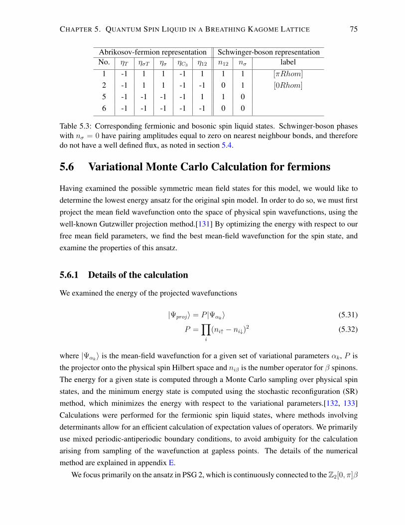
CHAPTER 5. QUANTUM SPIN LIQUID IN A BREATHING KAGOME LATTICE 75
Abrikosov-fermion representation Schwinger-boson representationNo. ηT ησT ησ ηC3 η12 n12 nσ label1 -1 1 1 -1 1 1 1 [πRhom]
2 -1 1 1 -1 -1 0 1 [0Rhom]
5 -1 -1 -1 -1 1 1 06 -1 -1 -1 -1 -1 0 0
Table 5.3: Corresponding fermionic and bosonic spin liquid states. Schwinger-boson phaseswith nσ = 0 have pairing amplitudes equal to zero on nearest neighbour bonds, and thereforedo not have a well defined flux, as noted in section 5.4.
5.6 Variational Monte Carlo Calculation for fermions
Having examined the possible symmetric mean field states for this model, we would like todetermine the lowest energy ansatz for the original spin model. In order to do so, we must firstproject the mean field wavefunction onto the space of physical spin wavefunctions, using thewell-known Gutzwiller projection method.[131] By optimizing the energy with respect to ourfree mean field parameters, we find the best mean-field wavefunction for the spin state, andexamine the properties of this ansatz.
5.6.1 Details of the calculation
We examined the energy of the projected wavefunctions
|Ψproj〉 = P |Ψαk〉 (5.31)
P =∏i
(ni↑ − ni↓)2 (5.32)
where |Ψαk〉 is the mean-field wavefunction for a given set of variational parameters αk, P isthe projector onto the physical spin Hilbert space and niβ is the number operator for β spinons.The energy for a given state is computed through a Monte Carlo sampling over physical spinstates, and the minimum energy state is computed using the stochastic reconfiguration (SR)method, which minimizes the energy with respect to the variational parameters.[132, 133]Calculations were performed for the fermionic spin liquid states, where methods involvingdeterminants allow for an efficient calculation of expectation values of operators. We primarilyuse mixed periodic-antiperiodic boundary conditions, to avoid ambiguity for the calculationarising from sampling of the wavefunction at gapless points. The details of the numericalmethod are explained in appendix E.
We focus primarily on the ansatz in PSG 2, which is continuously connected to the Z2[0, π]β

CHAPTER 5. QUANTUM SPIN LIQUID IN A BREATHING KAGOME LATTICE 76
phase. Examination of the energies of wavefunctions in other PSGs show consistently higherenergies. We examine the mean field wavefunction with up to second neighbour non-zero am-plitudes. Nearest neighbour hopping χ4 is fixed to 1 (4 denotes the up triangles), and weuse the gauge freedom to set ∆4 to 0. We thus have six free parameters in our minimization:on-site chemical potentials µ and η, nearest neighbour hopping and pairing χ∇ and ∆∇ andsecond nearest neighbour hopping and pairing χ2 and ∆2.
Calculations were performed on a 768 site lattice (16x16x3). The wavefunction was con-sidered minimized when the effective forces (i.e. the change in energy with respect to thevariational parameters, calculated within the SR scheme) averaged out to zero over a largenumber of runs.
5.6.2 Results
A number of important differences appear between the ansatze for the isotropic and anisotropickagome lattices. In particular, comparing the most general ansatz for the Z2[0, π]β phase andthe ansatz for spin liquids in PSG 2, two additional parameters appear in PSG 2; namely, χ∇and ∆∇, which encode the breaking of the rotational symmetry from C6 down to C3. Bysetting χ∇ = 1 and ∆∇ = 0, we recover the isotropic ansatz; this provides a useful upper limitto our energy per site of E = −0.42872(J4+ J∇)/2 found in previous studies of the isotropickagome lattice, which found a U(1) ground state.[108] In addition, this provides an additionalavenue for breaking of the U(1) symmetry down to Z2; if any of the parameters ∆∇, ∆2 or ηare non-zero in the minimized ansatz, the ansatz represents a Z2 state. More importantly, theanisotropy in the variational parameters and the presence of additional variational parametersis expected to change the ground state configuration of all parameters.
Our main result is that with the increase of anisotropy between the inequivalent triangles,the Z2 phase becomes the clear ground state within the VMC calculation. We determine thisusing two complementary approaches; first, we determine directly the energetic minimum fromthe SR procedure on the full parameter space, and, secondly, we minimize the energies atvarious fixed values of ∆2, showing directly that the energetic minimum occurs for a non-zerovalue of ∆2.
By considering the converged result of a large number of SR minimizations we can de-termine the values of the mean field parameters which we are varying. In the regime 0.5 ≤J∇/J4 ≤ 0.8, the variational parameters clearly converge to a single result, which yields agapped wavefunction with a Z2 gauge structure. Shown in Fig. 5.7 is a typical optimizationrun in the case J∇/J4 = 0.7; here we see a clear convergence of the U(1) symmetry breakingparameters ∆2 and η to non-zero values. For the converged order parameters, we find values

CHAPTER 5. QUANTUM SPIN LIQUID IN A BREATHING KAGOME LATTICE 77
µ
ηχ∇∆∇χ2
∆2
Figure 5.7: A typical optimization run for the parameters, at anisotropy J∇/J4 = 0.7. Thefact that η and ∆2 are non-zero implies that this is a Z2 spin liquid.
of µ = 0.802(1), η = 0.116(5), χ∇ = 0.715(2), ∆∇ = 0.000(2), χ2 = −0.0174(1) and∆2 = −0.0331(2).
The fact that ∆∇ appears to be zero (within error bars) is not determined by the projec-tive symmetry group of the ansatz, but rather is a property of the solution. Interestingly, thisis required in the Z2[0, π]β phase explored for the isotropic kagome lattice, suggesting thatour minimum energy state is highly similar to the state found in the isotropic lattice. Theground state ansatz does not, however, directly correspond to this state, as the symmetry break-ing between the hopping parameters on inequivalent triangles (χ∇/χ4 = .715) removes thispossibility.
We next explore the energies of the ansatz with ∆2 fixed to a number of non-zero values, inorder to directly confirm the breaking of the U(1) symmetry. Although the energy differencesare small, they can be detected by performing a sufficiently large number of uncorrelated sim-ulations. In Fig. 5.8, we show the minimum energy of the variational state as a function of∆2, which confirms that the U(1) state is higher in energy than the minimum energy Z2 state.A gauge symmetry relates positive and negative ∆2; as such, we plot this as a function of theabsolute value of this parameter.
This result, that the ground state of the anisotropic kagome lattice is a Z2 spin liquid,appears to be robust against the varying of the specific details of the calculation. The re-sults shown are for a 768 site lattice with mixed boundary conditions at an anisotropy ofJ∇/J4 = 0.7. Smaller lattice sizes were also explored, with 12x12x3, 8x8x3 and 4x4x3lattices all showing results which are consistent with those found on the larger system size. Forsystems with anisotropy approaching the isotropic limit, numerical issues with multiple possi-ble minima prevented convergence of the calculation. However, with anisotropy in the rangelisted (0.5 ≤ J∇/J4 ≤ 0.8), the convergence was clear and unambiguous. Finally, while pe-
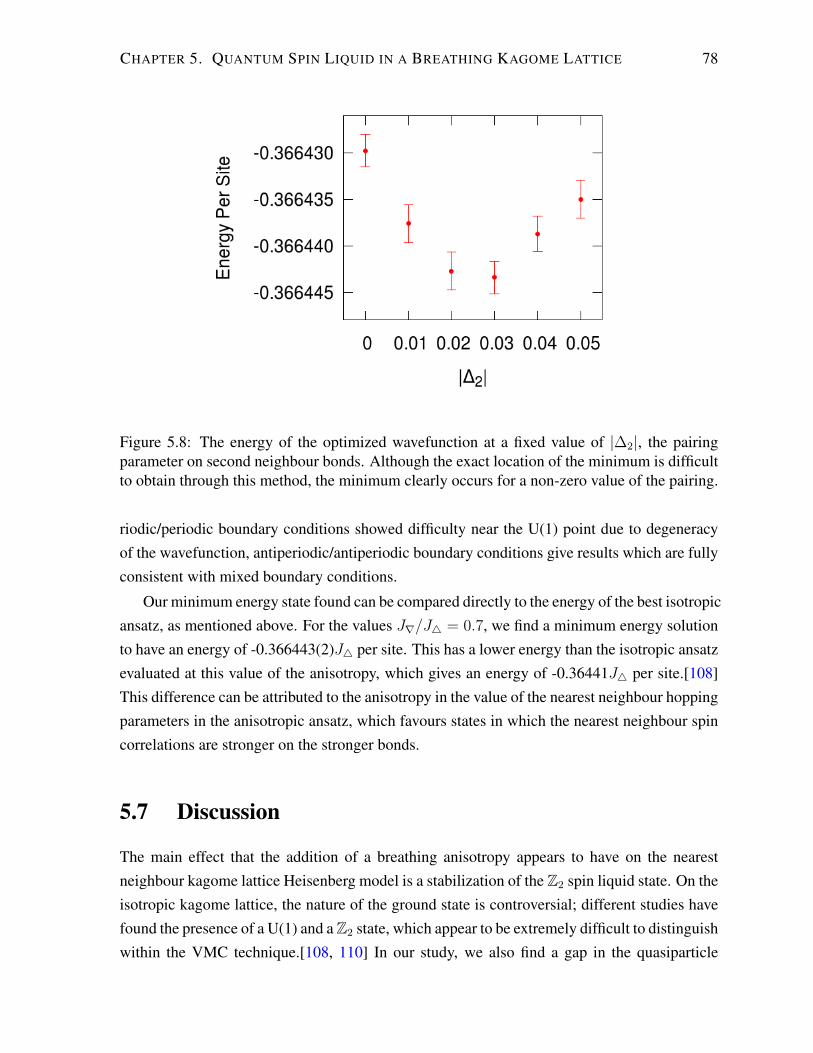
CHAPTER 5. QUANTUM SPIN LIQUID IN A BREATHING KAGOME LATTICE 78
Figure 5.8: The energy of the optimized wavefunction at a fixed value of |∆2|, the pairingparameter on second neighbour bonds. Although the exact location of the minimum is difficultto obtain through this method, the minimum clearly occurs for a non-zero value of the pairing.
riodic/periodic boundary conditions showed difficulty near the U(1) point due to degeneracyof the wavefunction, antiperiodic/antiperiodic boundary conditions give results which are fullyconsistent with mixed boundary conditions.
Our minimum energy state found can be compared directly to the energy of the best isotropicansatz, as mentioned above. For the values J∇/J4 = 0.7, we find a minimum energy solutionto have an energy of -0.366443(2)J4 per site. This has a lower energy than the isotropic ansatzevaluated at this value of the anisotropy, which gives an energy of -0.36441J4 per site.[108]This difference can be attributed to the anisotropy in the value of the nearest neighbour hoppingparameters in the anisotropic ansatz, which favours states in which the nearest neighbour spincorrelations are stronger on the stronger bonds.
5.7 Discussion
The main effect that the addition of a breathing anisotropy appears to have on the nearestneighbour kagome lattice Heisenberg model is a stabilization of the Z2 spin liquid state. On theisotropic kagome lattice, the nature of the ground state is controversial; different studies havefound the presence of a U(1) and a Z2 state, which appear to be extremely difficult to distinguishwithin the VMC technique.[108, 110] In our study, we also find a gap in the quasiparticle

CHAPTER 5. QUANTUM SPIN LIQUID IN A BREATHING KAGOME LATTICE 79
spectrum, which implies a gap for the spin excitations in the model.While the anisotropy leads to the reduction of the number of spin liquids present in the PSG,
more freedom is allowed in the choice of parameters present, leading to an overall increase inthe set of possible wavefunctions which satisfy the symmetries of the lattice. Within these, wefind a state which continuously connects to the Z2[0, π]β phase to be the energetically favouredground state.
The isotropic kagome lattice has been studied using other numerical methods, most notablythe density matrix renormalization group (DMRG). Strong evidence of a Z2 spin liquid groundstate has been found in entanglement entropy measurements using this method; however, anadditional second neighbour Heisenberg spin interaction for the unambiguous identification ofthis state, as the purely nearest neighbour model appears to be near a critical regime.[107] Ourstudy suggests that adding a breathing anisotropy to the Hamiltonian may offer another pathto stabilizing the Z2 spin liquid phase, and therefore offers a worthwhile direction for furthernumerical studies. In particular, while our study indicates that a gapped spin liquid is the likelyground state for this model, estimating the magnitude of the singlet gap which may appearin experiments is a challenge which would require a DMRG study. Such a spin gap estimatecould be compared to experimental results, offering evidence for this state being realized inmaterials such as DQVOF.

Chapter 6
Conclusion
In this thesis, we have explored a variety of the properties of spin liquids in certain Kitaev andkagome systems. However, much work remains to be done, as these systems have proven timeand time again to be rich in fascinating physics. Here, we discuss what has been done in thiswork, and some possible avenues to explore in future research.
6.1 Summary
In chapter 2, we explored the Heisenberg-Kitaev model on the honeycomb lattice. Of particularinterest to us is the nature of the quantum phase transition between the gapless Z2 spin liquidphase and the stripy magnetically ordered phase. In order to study this we use a slave particlemean field theory, through which we find a discontinuous transition. We argue that subtlespinon confinement effects, associated with the instability of gapped U(1) spin liquid in twospatial dimensions, play an important role at this transition.
Next, in chapter 3, we discussed the Kitaev model on a pair of recently discovered three-dimensional lattices, the hyper-honeycomb andH–1 lattices. The exact solution remains robuston these lattices, which allows us to directly examine the topological and surface properties.We find a nodal line spectrum of Majorana excitations, which remains protected in the absenceof symmetry breaking perturbations. In addition, topologically protected surface flat bandsmust appear. This state is expected to persist to finite temperatures, and a number of possibleexperiments have been proposed to examine this order.
Following this, we discuss the possible form of spin-orbital liquids which appear in pseudo-spin 1/2 doublets which appear due to crystalline symmetries rather than time reversal symme-try, in chapter 4. We examine this on the kagome lattice, where we find ten new phases that arenot allowed in the corresponding Kramers systems. We compute the spin-spin dynamic struc-ture factor that shows characteristic features of these non-Kramers spin-orbital liquids arising
80

CHAPTER 6. CONCLUSION 81
from their unusual coupling to neutrons, which is therefore relevant for neutron scattering ex-periments. We also point out possible anomalous broadening of Raman scattering intensity thatmay serve as a signature experimental feature for gapless non-Kramers spin-orbital liquids.
Finally, in chapter 5, we examine possible spin liquid phases on a breathing kagome latticeof S=1/2 spins. We first establish the possible phases in the bosonic and fermionic mean fieldtheories, as well as the correspondence between the two. The nature of the ground state ofthe Heisenberg model on the isotropic kagome lattice is a hotly debated topic, with both Z2
and U(1) spin liquids argued to be plausible ground states. Using variational Monte Carlotechniques, we show that a gapped Z2 spin liquid emerges as the clear ground state in thepresence of this breathing anisotropy. In addition to possible application to DQVOF, our resultssuggest that the breathing anisotropy helps to stabilize this spin liquid ground state, which mayaid us in understanding the results of experiments and help to direct future numerical studieson these systems.
6.2 Future Directions
In the works described above, as in spin liquid research as a whole, many open questionsremain. Here, we mention two possible avenues to explore in future research.
In the Heisenberg-Kitaev model on the honeycomb lattice, the transition between the stripyphase and the spin liquid appears to be first order, within our mean field calculation. However,we know that this story may be incomplete, due to the mean field approximation being made,and numerical studies have indicated the possibility of a continuous transition in this system.A field theoretical model of this transition, if attained, may allow for an unconventional contin-uous transition, which could shed light on experiments probing a system which may be closeto the spin liquid phase.
In the Heisenberg model on the breathing kagome lattice, the spin liquid phase appears tostabilize with the inclusion of a breathing anisotropy, relative to the isotropic case. This offers avaluable direction to explore in future numerical studies, which have had difficulty determiningunambiguously the nature of the isotropic ground state. In addition, our understanding of thematerial DQVOF would benefit from an estimate of the spin gap in this model, which could beobtained using DMRG.

Appendices
82

Appendix A
Crystal Field Effects in Pr2TM2O7
In this appendix, we explore the breaking of the J = 4 spin degeneracy by the crystallineelectric field. The oxygen and TM ions form a D3d local symmetry environment around thePr3+ ions, splitting the ground state degeneracy of the electrons. This symmetry group con-tains 6 classes of elements: E, 2C3, 3C ′2, i, 2S6, and 3σd, where the C3 are rotations by 2π/3
about the local z axis, the C ′2 are rotations by π about axis perpendicular to the local z axis, iis inversion, S6 is a rotation by 4π/3 combined with inversion and σd is a reflection about theplane connecting one corner and the opposing plane, running through the Pr molecule aboutwhich this is measured (or, equivalently, a rotation about the x axis combined with inversion).For our J=4 manifold, these have characters given by
χ(4)(E) = 2 ∗ 4 + 1 = 9 = χ(4)(i) (A.1)
χ(4)(C3) = χ(4)(2π
3) =
sin(3π)
sin(π/3)= 0 = χ(4)(S6) (A.2)
χ(4)(σd) = χ(4)(π) =sin(9π/2)
sin(π/2)= 1 = χ(4)(C ′2) (A.3)
where the latter equalities are given by the fact that our J=4 manifold is inversion symmetric.Thus, decomposing this in terms of D3d irreps, our J=4 manifold splits into a sum of doubletand singlet manifolds as
ΓJ=4 = 3Eg + 2A1g + A2g. (A.4)
To examine this further, we need to consider the matrix elements of the crystal field po-tential between the states of different angular momenta. We know that this potential must beinvariant under all group operations of D3d, so we can examine the transformation propertiesof individual matrix elements, 〈m|V |m′〉. Under the C3 operation, these states of fixed m
83
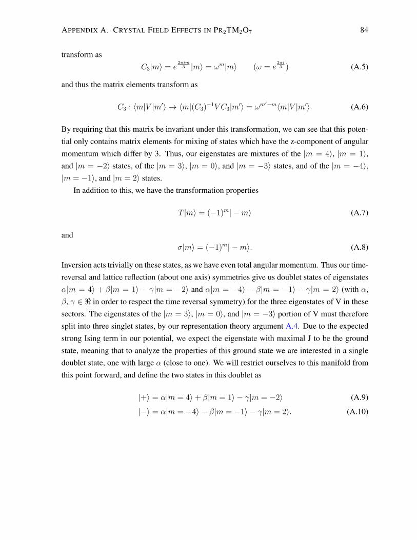
APPENDIX A. CRYSTAL FIELD EFFECTS IN PR2TM2O7 84
transform asC3|m〉 = e
2πim3 |m〉 = ωm|m〉 (ω = e
2πi3 ) (A.5)
and thus the matrix elements transform as
C3 : 〈m|V |m′〉 → 〈m|(C3)−1V C3|m′〉 = ωm′−m〈m|V |m′〉. (A.6)
By requiring that this matrix be invariant under this transformation, we can see that this poten-tial only contains matrix elements for mixing of states which have the z-component of angularmomentum which differ by 3. Thus, our eigenstates are mixtures of the |m = 4〉, |m = 1〉,and |m = −2〉 states, of the |m = 3〉, |m = 0〉, and |m = −3〉 states, and of the |m = −4〉,|m = −1〉, and |m = 2〉 states.
In addition to this, we have the transformation properties
T |m〉 = (−1)m| −m〉 (A.7)
andσ|m〉 = (−1)m| −m〉. (A.8)
Inversion acts trivially on these states, as we have even total angular momentum. Thus our time-reversal and lattice reflection (about one axis) symmetries give us doublet states of eigenstatesα|m = 4〉 + β|m = 1〉 − γ|m = −2〉 and α|m = −4〉 − β|m = −1〉 − γ|m = 2〉 (with α,β, γ ∈ < in order to respect the time reversal symmetry) for the three eigenstates of V in thesesectors. The eigenstates of the |m = 3〉, |m = 0〉, and |m = −3〉 portion of V must thereforesplit into three singlet states, by our representation theory argument A.4. Due to the expectedstrong Ising term in our potential, we expect the eigenstate with maximal J to be the groundstate, meaning that to analyze the properties of this ground state we are interested in a singledoublet state, one with large α (close to one). We will restrict ourselves to this manifold fromthis point forward, and define the two states in this doublet as
|+〉 = α|m = 4〉+ β|m = 1〉 − γ|m = −2〉 (A.9)
|−〉 = α|m = −4〉 − β|m = −1〉 − γ|m = 2〉. (A.10)

Appendix B
Fermion PSG solution for isotropickagome lattice
B.1 Gauge transformations
We begin by describing the action of time reversal on our ansatz. The operation is antiunitary,and comes with a spin transformation σ1 in the case of non-Kramers doublets. As a result,the operation acts as T : ξαβij ΣαΓβ → ξαβ∗ij Σ1Σα∗Σ1Γβ∗. However, we can simplify thisconsiderably by performing a gauge transformation in addition to the above transformation,which yields the same transformation on any physical variables. The gauge transformation weperform is iΓ2, which changes the form of the time reversal operation to T : ξαβij ΣαΓβ →ξαβ∗ij Σ1Σα∗Σ1Γ2Γβ∗Γ2 = ξαβij ΣαΓβ , where ξαβ = ξαβ if α ∈ 1, 2 and ξαβ = −ξαβ if α ∈0, 3.
On the Kagome lattice, the allowed form of the gauge transformations has been determinedby Yuan-Ming Lu et al.[100] For completeness, we will reproduce that calculation, valid also
85

APPENDIX B. FERMION PSG SOLUTION FOR ISOTROPIC KAGOME LATTICE 86
for our spin triplet ansatz, here. The relations between the gauge transformation matrices,
[GT (i)]2 = ηT I, (B.1)
Gσ(σ(i))Gσ(i) = ησI, (B.2)
G†T1(i)G†T (i)GT1(i)GT (T−1
1 (i)) = ηT1T I, (B.3)
G†T2(i)G†T (i)GT2(i)GT (T−1
2 (i)) = ηT2T I, (B.4)
G†σ(i)G†T (i)Gσ(i)GT (σ−1(i)) = ησT I, (B.5)
G†S6(i)G†T (i)GS6(i)GT (S−1
6 (i)) = ηS6T I, (B.6)
G†T2(T−11 (i))G†T1(i)GT2(i)GT1(T
−12 (i)) = η12I, (B.7)
GS6(S−16 (i))GS6(S
−26 (i))GS6(S
36(i))
×GS6(S26(i))GS6(S6(i))GS6(i) = ηS6I, (B.8)
G†σ(T−12 (i))G†T2(i)Gσ(i)GT1(σ(i)) = ησT1I, (B.9)
G†σ(T−11 (i))G†T1(i)Gσ(i)GT2(σ(i)) = ησT2I, (B.10)
G†σ(S6(i))GS6(S6(i))Gσ(i)GS6(σ(i)) = ησS6I, (B.11)
G†S6(T−1
2 (i))G†T2(i)GS6(i)GT1(S−16 (i)) = ηS6T1I, (B.12)
G†S6(T−1
2 T1(i))G†T2(T1(i))GT1(T1(i))
GS6(i)GT2(S−16 (i)) = ηS6T2I, (B.13)
are valid for our case as well, due to the decoupling of spin and gauge portions of our ansatz.In the above, the relations are valid for all lattice sites i = (x, y, s), I is the 4x4 identity matrix,and the GS matrices are gauge transformation matrices generated by exponentiation of the Γ
matrices. The η’s are ±1, the choice of which characterize different spin liquid states.
We turn next to the calculation of the gauge transformations. We look first at the gaugetransformations associated with the translations. We can perform a site dependent gauge trans-formation W (i), under which the gauge transformations associated with the translational sym-metries transform as
GT1(i)→ W (i)GT1(i)W†(i− x) (B.14)
GT2(i)→ W (i)GT2(i)W†(i− y). (B.15)
As such, we can choose a gauge transformation W(i) to simplify the form of GT1 and GT2 .Using such a transformation, along with condition B.7, we can restrict the form of these gauge

APPENDIX B. FERMION PSG SOLUTION FOR ISOTROPIC KAGOME LATTICE 87
transformations to be
GT1(i) = ηiy12I GT2(i) = I. (B.16)
To preserve this choice, we can now only perform gauge transformations which are equiva-lent on all lattice positions (W (x, y, s) = W (s)) or transformations which change the shownmatrices by an IGG transformation.
Next, we look at adding the reflection symmetry σ. Given our formulae for GT1 and GT2 ,along with the relations between the gauge transformations, we have that
G†σ(T−12 (i))Gσ(i)ηx12 = ησT1I (B.17)
G†σ(T−11 (i))Gσ(i)ηy12 = ησT2I. (B.18)
Defining Gσ(0,0,s) = gσ(s), we have, by repeated application of the above,
Gσ(0, y, s) = ηyσT1gσ(s) (B.19)
Gσ(x, y, s) = ηyσT1ηxy12η
xσT2gσ(s). (B.20)
Next, using
Gσ(σ(i))Gσ(i) = ησI (B.21)
we find that
ησI = Gσ(y, x, σ(s))Gσ(x, y, s) (B.22)
= (ησT1ησT2)x+ygσ(σ(s))gσ(s). (B.23)
Since this is true for all x and y, ησT1ησT2 = 1 and thus ησT1 = ησT2 and gσ(σ(s))gσ(s) = ησI
(where σ(u) = u, σ(v) = w and σ(w) = v). Our final form for the gauge transformation is
Gσ(x, y, s) = ηx+yσT1
ηxy12 gσ(s). (B.24)
Next we look at adding the S6 symmetry to our calculation. We can do an IGG transfor-mation, taking GT1(T1(i)) to ηS6T2GT1(T1(i)), with the net effect being that ηS6T2 becomes one

APPENDIX B. FERMION PSG SOLUTION FOR ISOTROPIC KAGOME LATTICE 88
(previous calculations are unaffected). We now have that
G†S6(T−1
2 T1(i))GS6(i)ηy12 = I (B.25)
G†S6(T−1
2 (i))GS6(i)η−x−112 = ηS6T1I (s = u, v) (B.26)
G†S6(T−1
2 (i))GS6(i)η−x12 = ηS6T1I (s = w). (B.27)
Defining GS6(0, 0, s) = gS6(s), we find that
GS6(n,−n, s) = ηn(n−1)/212 gS6(s) (B.28)
GS6(x, y, s) = ηx(x−1)/2+y+xy12 ηx+y
S6T1gS6(s) (s = u, v) (B.29)
GS6(x, y, s) = ηx(x−1)/2+xy12 ηx+y
S6T1gS6(s) (s = w). (B.30)
Using the commutation relation between the σ and S6 gauge transformations, we find that
ησS6I = ηyσT1ηy12η
yS6T1
g†σ(v)gS6(v)gσ(u)gS6(u) (B.31)
= ηyσT1ηy12η
yS6T1
ησgσ(w)gS6(v)gσ(u)gS6(u) (B.32)
giving us that ησT1η12ηS6T1 = 1 and gσ(u)gS6(u)gσ(w)gS6(v) = ησS6ησI . A similar calculationon a different sublattice gives us
ησS6I = ηyσT1ηy12η
yS6T1
g†σ(w)gS6(w)gσ(v)gS6(w) (B.33)
= ηyσT1ηy12η
yS6T1
ησgσ(v)gS6(w)gσ(v)gS6(w) (B.34)
giving us (gσ(v)gS6(w))2 = ησS6ησI . AZ2 (IGG) gauge transformation of the formW (x, y, s) =
ηyσT1 changes ησT1 to 1. Using the cyclic relation of the gauge transformations related to the S6
operators, we find
ηS6I = η12(gS6(w)gS6(v)gS6(u))2 (B.35)
giving us that
[gS6(w)gS6(v)gS6(u)]2 = ηS6η12I. (B.36)
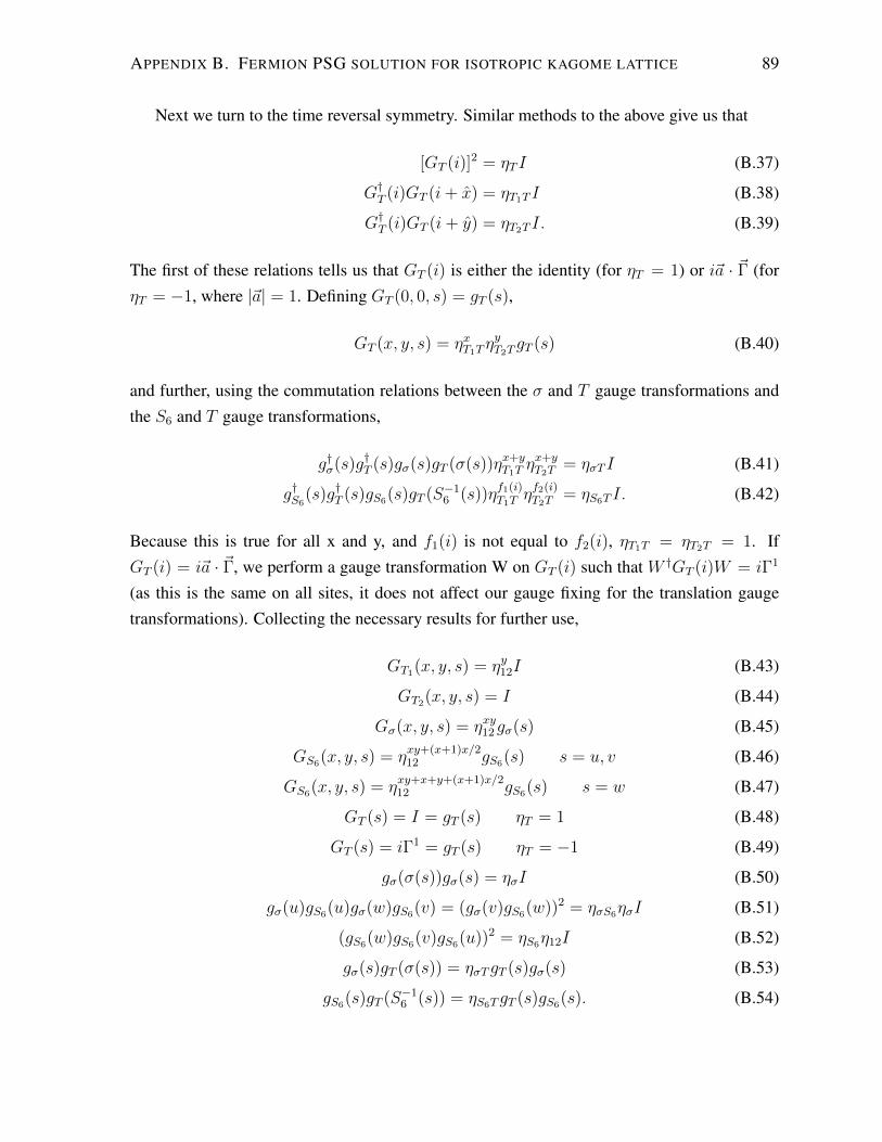
APPENDIX B. FERMION PSG SOLUTION FOR ISOTROPIC KAGOME LATTICE 89
Next we turn to the time reversal symmetry. Similar methods to the above give us that
[GT (i)]2 = ηT I (B.37)
G†T (i)GT (i+ x) = ηT1T I (B.38)
G†T (i)GT (i+ y) = ηT2T I. (B.39)
The first of these relations tells us that GT (i) is either the identity (for ηT = 1) or i~a · ~Γ (forηT = −1, where |~a| = 1. Defining GT (0, 0, s) = gT (s),
GT (x, y, s) = ηxT1TηyT2T
gT (s) (B.40)
and further, using the commutation relations between the σ and T gauge transformations andthe S6 and T gauge transformations,
g†σ(s)g†T (s)gσ(s)gT (σ(s))ηx+yT1T
ηx+yT2T
= ησT I (B.41)
g†S6(s)g†T (s)gS6(s)gT (S−1
6 (s))ηf1(i)T1T
ηf2(i)T2T
= ηS6T I. (B.42)
Because this is true for all x and y, and f1(i) is not equal to f2(i), ηT1T = ηT2T = 1. IfGT (i) = i~a · ~Γ, we perform a gauge transformation W on GT (i) such that W †GT (i)W = iΓ1
(as this is the same on all sites, it does not affect our gauge fixing for the translation gaugetransformations). Collecting the necessary results for further use,
GT1(x, y, s) = ηy12I (B.43)
GT2(x, y, s) = I (B.44)
Gσ(x, y, s) = ηxy12 gσ(s) (B.45)
GS6(x, y, s) = ηxy+(x+1)x/212 gS6(s) s = u, v (B.46)
GS6(x, y, s) = ηxy+x+y+(x+1)x/212 gS6(s) s = w (B.47)
GT (s) = I = gT (s) ηT = 1 (B.48)
GT (s) = iΓ1 = gT (s) ηT = −1 (B.49)
gσ(σ(s))gσ(s) = ησI (B.50)
gσ(u)gS6(u)gσ(w)gS6(v) = (gσ(v)gS6(w))2 = ησS6ησI (B.51)
(gS6(w)gS6(v)gS6(u))2 = ηS6η12I (B.52)
gσ(s)gT (σ(s)) = ησTgT (s)gσ(s) (B.53)
gS6(s)gT (S−16 (s)) = ηS6TgT (s)gS6(s). (B.54)

APPENDIX B. FERMION PSG SOLUTION FOR ISOTROPIC KAGOME LATTICE 90
Table B.1: We list the solutions of Eq. B.43 - B.54, along with a set of gauge transformationswhich realize these solutions.
No. ηT ησT ηS6T ησ ησS6 ηS6 η12 gσ(u) gσ(v) gσ(w) gS6(u) gS6(v) gS6(w)
1,2 -1 1 1 1 1 ±1 ±1 Γ0 Γ0 Γ0 Γ0 Γ0 Γ0
3,4 -1 1 1 1 -1 ∓1 ±1 Γ0 Γ0 Γ0 Γ0 -Γ0 iΓ1
5,6 -1 1 -1 1 -1 ∓1 ±1 Γ0 Γ0 Γ0 iΓ3 iΓ3 iΓ3
7,8 -1 1 1 -1 -1 ∓1 ±1 iΓ1 Γ0 -Γ0 Γ0 iΓ1 Γ0
9,10 -1 1 1 -1 1 ±1 ±1 iΓ1 Γ0 -Γ0 Γ0 -iΓ1 iΓ1
11,12 -1 1 -1 -1 1 ∓1 ±1 iΓ1 Γ0 -Γ0 iΓ3 -iΓ2 iΓ3
13,14 -1 -1 -1 -1 -1 ∓1 ±1 iΓ3 iΓ3 iΓ3 iΓ3 iΓ3 iΓ3
15,16 -1 -1 1 -1 1 ±1 ±1 iΓ3 iΓ3 iΓ3 Γ0 Γ0 Γ0
17,18 -1 -1 1 -1 1 ∓1 ±1 iΓ3 iΓ3 iΓ3 Γ0 Γ0 iΓ1
19,20 -1 -1 -1 -1 1 ∓1 ±1 iΓ3 iΓ3 iΓ3 iΓ3 -iΓ3 iΓ3
21,22 1 1 1 1 1 ±1 ±1 Γ0 Γ0 Γ0 Γ0 Γ0 Γ0
23,24 1 1 1 1 -1 ∓1 ±1 Γ0 Γ0 Γ0 Γ0 -Γ0 iΓ3
25,26 1 1 1 -1 -1 ∓1 ±1 iΓ3 Γ0 -Γ0 Γ0 iΓ3 Γ0
27,28 1 1 1 -1 1 ∓1 ±1 iΓ3 Γ0 -Γ0 Γ0 -iΓ3 iΓ1
29,30 1 1 1 -1 1 ±1 ±1 iΓ3 Γ0 -Γ0 Γ0 -iΓ3 iΓ3
We also have the gauge freedom left to perform a gauge rotation arbitrarily at all positions forηT = 1 or an arbitrary gauge rotation about the x axis for ηT = −1.
The solution to the above equations is derived in detail by Lu et al.[100] and as such wesimply list the results in table B.1. The basic method of obtaining these solutions is as follows:for each choice of Z2 parameter set, we determine whether there is a choice of gauge matrices gS which satisfy the equations B.43 - B.54. In order to do so, we determine the allowedforms of the gS matrices from the equations, then use the gauge freedom on each site to fix theform of these. Of particular note is the fact that in the consistency equations for the g matrices,the terms η12 and ηS6 only appear multiplied together, meaning that for any choice of the gaugematrices gS we can choose η12 = ±1, which fixes the form of ηS6 .
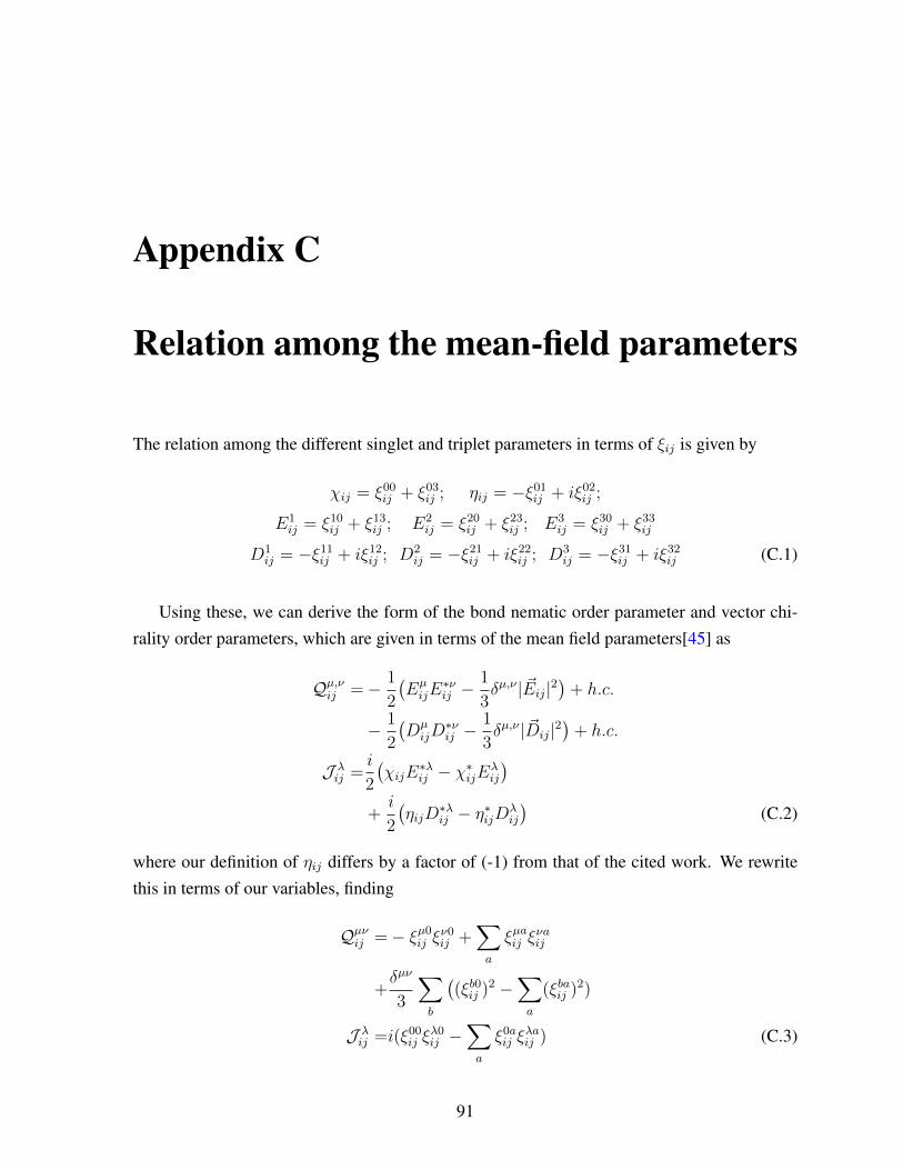
Appendix C
Relation among the mean-field parameters
The relation among the different singlet and triplet parameters in terms of ξij is given by
χij = ξ00ij + ξ03
ij ; ηij = −ξ01ij + iξ02
ij ;
E1ij = ξ10
ij + ξ13ij ; E2
ij = ξ20ij + ξ23
ij ; E3ij = ξ30
ij + ξ33ij
D1ij = −ξ11
ij + iξ12ij ; D2
ij = −ξ21ij + iξ22
ij ; D3ij = −ξ31
ij + iξ32ij (C.1)
Using these, we can derive the form of the bond nematic order parameter and vector chi-rality order parameters, which are given in terms of the mean field parameters[45] as
Qµ,νij =− 1
2
(EµijE∗νij −
1
3δµ,ν | ~Eij|2
)+ h.c.
− 1
2
(DµijD
∗νij −
1
3δµ,ν | ~Dij|2
)+ h.c.
J λij =
i
2
(χijE
∗λij − χ∗ijEλ
ij
)+i
2
(ηijD
∗λij − η∗ijDλ
ij
)(C.2)
where our definition of ηij differs by a factor of (-1) from that of the cited work. We rewritethis in terms of our variables, finding
Qµνij =− ξµ0ij ξ
ν0ij +
∑a
ξµaij ξνaij
+δµν
3
∑b
((ξb0ij )2 −
∑a
(ξbaij )2)
J λij =i(ξ00
ij ξλ0ij −
∑a
ξ0aij ξ
λaij ) (C.3)
91

APPENDIX C. RELATION AMONG THE MEAN-FIELD PARAMETERS 92
In particular, we find that J 1, J 2, Q13 and Q23 must be zero for all non-Kramers spin liquids,as the terms allowed by symmetry in Eq. 4.33 and 4.34 do not allow non-zero values for theseorder parameters.
Appendix D
Full PSG solution for anisotropic kagomelattice
The anisotropic kagome lattice lies in the space group p3m1, which can be generated by foursymmetries, T1, T2, σ, C3. A convenient presentation for this space group has eight relationsbetween these generators,
σ2 = e (D.1)
T−12 T−1
1 T2T1 = e (D.2)
C33 = e (D.3)
σ−1T−12 σT1 = e (D.4)
σ−1T−11 σT2 = e (D.5)
C3σC3σ = e (D.6)
C−13 T−1
2 T1C3T1 = e (D.7)
C−13 T1C3T2 = e. (D.8)
As described in the main text, the mean field Hamiltonian must be invariant under a combi-nation of symmetry operations and gauge transformations, in order for the physical wavefunc-tion to respect the symmetries. Considering sets of symmetry operations whose product is the
93

APPENDIX D. FULL PSG SOLUTION FOR ANISOTROPIC KAGOME LATTICE 94
identity leads to relations between the gauge transformations, which take the form
Gσ(σ(i))Gσ(i) = ησI, (D.9)
G†T2(T−11 (i))G†T1(i)GT2(i)GT1(T
−12 (i)) = η12I, (D.10)
GC3(C23(i))GC3(C3(i))GC3(i) = ηC3I, (D.11)
G†σ(T−12 (i))G†T2(i)Gσ(i)GT1(σ(i)) = ησT1I, (D.12)
G†σ(T−11 (i))G†T1(i)Gσ(i)GT2(σ(i)) = ησT2I, (D.13)
GC3(C3σ(i))Gσ(σ(i))GC3(i)Gσ(C−13 (i)) = ησC3I, (D.14)
G†C3(T−1
2 T1(i))G†T2(T1(i))GT1(T1(i))
×GC3(i)GT1(C−13 (i)) = ηC3T1I, (D.15)
G†C3(T1(i))GT1(T1(i))GC3(i)GT2(C
−13 (i)) = ηC3T2I. (D.16)
Each of the η’s above take values ±1, as the IGG which we consider is Z2.
The above relations which do not involve the rotation C3 are equivalent to those found onthe isotropic kagome lattice. The solution for these is therefore the same as on that lattice,which we will briefly recount here.
As with all two-dimensional lattices, we can perform a site dependent gauge transformationW (i) which restricts the gauge transformations associated with the translational symmetries to
GT1(x, y, s) = ηy12I, GT2(x, y, s) = I. (D.17)
Here (and further on) I denotes the 2x2 identity matrix for the fermionic transformations, and 1for the bosonic transformations. Any future gauge transformations must preserve these choices,up to an overall factor of ±1 which has no effect on the ansatz Uij .
The relations D.12 and D.13 restrict the gauge transformation Gσ to take the form
Gσ(0, y, s) = ηyσT1gσ(s) (D.18)
Gσ(x, y, s) = ηyσT1ηxσT2ηxy12 gσ(s), (D.19)
where gσ(s) is defined as Gσ(0, 0, s). Equation D.9 then requires
ησI = (ησT1ησT2)x+ygσ(σ(s))gσ(s). (D.20)
Because these relations must hold for all lattice positions x and y,
ησT1ησT2 = 1 (D.21)

APPENDIX D. FULL PSG SOLUTION FOR ANISOTROPIC KAGOME LATTICE 95
andgσ(σ(s))gσ(s) = ησI (D.22)
(where σ(u) = u, σ(v) = w and σ(w) = v).
At this point, we look to add the rotational symmetry C3. Before we solve the gauge matrixequations, we note that we have the freedom to multiply any of the gauge transformations byelements of the IGG, as a gauge transformation. Due to the fact that we are examining Z2 spinliquids, we can make the transformation
GT2 = ηC3T1GT2 , (D.23)
GT1 = ηC3T1ηC3T2GT1 , (D.24)
GC3 = −ηC3GC3 (D.25)
resulting in the fixing of the variables ηC3T1 , ηC3T2 and ηC3 .
Next, we wish to write GC3 as a product of a term which depends only on sublattice and aterm which depends only on lattice position, as we did for Gσ. We note that eq. D.15 and D.16can be rewritten as
G†C3(T−1
2 T1(i))GC3(i)ηx+112 = I, (D.26)
G†C3(T1(i))GC3(i)η
y12 = I, (D.27)
which, substituting GC3(0, 0, s) = −gC3(s), leads to
GC3(n,−n, s) = −ηn(n−1)/212 gC3(s), (D.28)
GC3(x, y, s) = −ηy(y+1)/2+y(x+y)12 gC3(s). (D.29)
Having the forms of Gσ and GC3 , we can consider the relations Eq. D.14 and D.11. Eq.D.14 simplifies to
ησC3I = ηy+1σT1
gC3(σ(s))gσ(σ(s))gC3(s)gσ(C−13 (s)) (D.30)
which tells us that ησT1 = 1, as both sides of this equation must be y independent. Consideringthe different sublattice indices, we find
ησC3I = gC3(w)gσ(u)gC3(u)gσ(v) (D.31)
= gC3(v)gσ(w)gC3(v)gσ(w). (D.32)

APPENDIX D. FULL PSG SOLUTION FOR ANISOTROPIC KAGOME LATTICE 96
Eq. D.11 simplifies to
η12gC3(u)gC3(v)gC3(w) = I. (D.33)
It is then convenient to make the further gauge transformation GC3 → η12GC3 , which removesη12 from Eq. D.33.
When considering the time reversal operation, it is convenient to consider bosonic andfermionic spin liquids separately. In the case of fermionic spin liquids, we consider the timereversal operator adjoined to a gauge transformation iτ2 rather than the bare operator (where~τ represents the vector of Pauli matrices). As iτ2 is a gauge transformation, it has no physicaleffect, but the ansatz now transforms as TUijT−1 = −Uij . This combined operator satisfiesT 2 = e and S−1T−1ST = e. In addition, this operator acting on a pure gauge transformationsatisfies TGT−1 = G, and can therefore be considered adjoined to a gauge transformation inthe same fashion as we considered other space group symmetries,
[GT (i)]2 = ηT I, (D.34)
G†T1(i)G†T (i)GT1(i)GT (T−1
1 (i)) = ηT1T I, (D.35)
G†T2(i)G†T (i)GT2(i)GT (T−1
2 (i)) = ηT2T I, (D.36)
G†σ(i)G†T (i)Gσ(i)GT (σ−1(i)) = ησT I, (D.37)
G†C3(i)G†T (i)GC3(i)GT (C−1
3 (i)) = ηC3T I, . (D.38)
Eq. D.35 and D.36 restrict GT (x, y, s) = ηxT1TηyT2T
gT (s), where gT (s) = GT (0, 0, s). Eq.D.37 then implies
g†σ(s)g†T (s)gσ(s)gT (σ(s))ηx+yT1T
ηx+yT2T
= ησT I (D.39)
leading to ηT1T = ηT2T . Considering next Eq. D.38, we find
g†C3(s)g†T (s)gC3(s)gT (C−1
3 (s))ηy+1T1T
= ηC3T I (D.40)
giving us also that ηT1T = 1. As such, GT (x, y, s) = gT (s).
Because TUijT−1 = −Uij , we require Uij = −GT (i)UijG†T (j). As the lattice is not
bipartite and we require the ansatz to be non-zero on all bonds, this requires GT (x, y, s) =
gT (s) = i~a · ~τ , implying ηT = 1. We perform a sublattice dependent gauge transformation Ws
on each sublattice, such thatWsgT (s)W †s = iτ2. We further note that ηC3T must always be 1, as
g†C3(s)τ2gC3(s)τ2 = −1 ∀s is incompatible with D.33. The remaining commutation equation

APPENDIX D. FULL PSG SOLUTION FOR ANISOTROPIC KAGOME LATTICE 97
simplifies tog†σ(s)τ2gσ(s)τ2 = ησT I. (D.41)
A sublattice dependent gauge transformation Ws = eiθsτ2 can be performed on each site,without affecting the previous results. This results in a change of the sublattice portions of thegauge transformations,
gσ(u)→ Wugσ(u)W †u , (D.42)
gσ(v)→ Wvgσ(v)W †w, (D.43)
gσ(w)→ Wwgσ(w)W †v , (D.44)
gC3(u)→ WugC3(u)W †v , (D.45)
gC3(v)→ WvgC3(v)W †w, (D.46)
gC3(w)→ WwgC3(w)W †u . (D.47)
We must now solve the equations D.22, D.31, D.32, D.33 and D.41. We note that ηC3T =
1 ⇒ gC3(s) = eiτ2θs , with θs ∈ [0, 2π). Using the gauge transformations Wu = e−iθuτ2 andWw = eiθvτ2 results in a fixing gC3(s) = I .
Manipulating Eq. D.22, D.31 and D.32 with gC3(s) = I we see that gσ(u) = gσ(w). Thisfurther implies that ησ = ησC3 , and therefore gσ(v) = gσ(u).
Different solutions arise for ησT = ±1. When ησT = 1, eq. D.41 gives gσ(s) = eiτ2φ forsome φ ∈ [0, 2π). This is further restricted by D.22 to gσ(s) = ±I for ησ = 1 or gσ(s) = ±iτ2
for ησ = −1. Finally, we can choose the positive solution for each of these, by performingthe gauge transformation Gσ → ±Gσ. When ησT = −1, eq. D.41 requires gσ(s) = iτ3e
iτ2φ
for some φ ∈ [0, 2π). Using the gauge transformation Wu = Wv = Ww = eiτ2φ/2, we can fixgσ(s) = iτ3. This gives a total of three solutions to the sublattice dependent equations, each ofwhich can have η12 = ±1. Therefore, we have six PSGs, the details of which are summarizedin table 5.1.
Next we describe the bosonic PSG. All of the solution prior to the consideration of timereversal is equivalent for bosons. In the bosonic case, we can solve the equations D.22, D.31,D.32 and D.33 directly, and show that these solutions are compatible with the time reversalsymmetry.
First, we note that the sublattice dependent gauge transformation Ws = eiθs is allowed forbosons, which have the same effect (Eq. D.42 - D.47) as for the fermionic operators. DenotinggS(s) = eiφS(s) and ηα = einα , we see from D.22 that φσ(u) = nσπ/2. Further, performing agauge transformation θv = (φσ(w)− φσ(v))/2, we can fix φσ(v) = φσ(w) = φσ(u) = nσπ/2.
Next, we see from eq. D.31 and D.32 that φ3(w) + φ3(u) = (nσC3 − nσ)π and φ3(v) =

APPENDIX D. FULL PSG SOLUTION FOR ANISOTROPIC KAGOME LATTICE 98
(nσC3−nσ)π/2. Combined with eq. D.33, we see that nσ = nσC3 , and therefore we can chooseφ3(v) = 0 and φ3(u) = φ3(w). Performing a gauge transformation θu = −φ3(u), we arrive atφ3(u) = φ3(v) = φ3(w) = 0.
Finally, we consider the effect of time reversal for bosons. Due to the condition φ3(s) = 0,all of the bonds on each type of triangle must have the same complex phase. Using an overallgauge transformation on each site on the lattice, we can enforce the condition that these are allreal on one type of triangle. In this gauge, it is clear that time reversal acts non-projectively.Thus, an ansatz satisfies the time reversal symmetry iff the other triangle is also real in thisgauge.

Appendix E
Details of the Variational Monte Carlocalculation
E.1 Mean Field theory
As described in chapter 5, the mean field Hamiltonian takes the form
H0 =∑ij
Jij ~fi†Uij ~fj +
∑i
3∑l=1
Λl ~fi†τ l ~fi
Uij =
[χ†ij ∆ij
∆†ij −χij
], ~fi =
[fi↑
f †i↓
](E.1)
where the τ l represent Pauli matrices. It is convenient to define the operators
~ψi =
[ψi1
ψi2
]≡
[fi↑
f †i↓
], (E.2)
which represent the f fermions described above with a particle hole transformation on the downspin fermions only. These obey the fermionic commutation relations ψ†iα, ψjβ = δijδαβ ,ψ†iα, ψ
†jβ = ψiα, ψjβ = 0, and therefore represent the same fermionic objects. How-
ever, in this basis, it is apparent that the Hamiltonian conserves the ψ-fermion number Nψ ≡∑iα ψ
†iαψiα. The physical requirement that one f -fermion appears on each site is equivalent to
a requirement that zero or two ψ-fermions appear on each site.
In terms of the spin operators, we see that
Szi =1
2(f †i↑fi↑ − f
†i↓fi↓) =
1
2(ψ†i1ψi1 + ψ†i2ψi2 − 1) =
1
2(Nψi − 1). (E.3)
99

APPENDIX E. DETAILS OF THE VARIATIONAL MONTE CARLO CALCULATION 100
The sum
Sztot =∑i
Siz =1
2
∑i
(Nψi − 1) =1
2(Nψ −Nsites) (E.4)
is invariant under the Hamiltonian. As such, by fixing the total ψ-fermion number in our sys-tem, we fix the total Sz in the states which we explore. This can be done for any physical valueof Sz. In particular, if we wish to explore states in the absence of spin rotational symmetrybreaking, we fix the total fermion number Nψ = Nsites.
The mean field Hamiltonian, in terms of ψ fermions, appears as
H0 =∑ij
Jij ~ψi†Uij ~ψj +
∑i
3∑l=1
Λl ~ψi†τ l ~ψi. (E.5)
This Hamiltonian can be diagonalized using a unitary transformation
ψiα =∑β
Viαβγβ. (E.6)
As this is a unitary transformation, the new operators γβ obey fermion commutation relations.The transformed Hamiltonian takes the form
H0 =∑β
εβγ†βγβ, (E.7)
where the εβ represent the eigenvalues ofH0. We choose a labelling of the eigenvalues ofH0 inincreasing order, such that ε1 ≤ ε2 ≤ ... ≤ ε2Nsites . In addition, the total γ-fermion occupationnumber is equal to the total ψ-fermion occupation number.
We can now construct the mean field ground state for a particular choice of the ansatz Uijwith a particular total Sz as a product state of the Nψ lowest energy fermions acting on thefermionic vacuum, i.e.
|ΨMF〉 = γ†1γ†2 · · · γ
†Nψ|0〉. (E.8)
However, this state is not uniquely defined if it is degenerate at the Fermi level, i.e. εNψ =
εNψ+1. In principle, this introduces a substantial complication to any calculation involving themean field ground state. In practice, by choosing antiperiodic boundary conditions we cantypically remove this degeneracy and focus on a uniquely defined ground state. In the eventthat this is unsuccessful, a more careful analysis is typically required. However, in the stateswhich we explored, this method was sufficient to remove the degeneracy, and therefore this

APPENDIX E. DETAILS OF THE VARIATIONAL MONTE CARLO CALCULATION 101
will not be explored further here.
E.2 Variational Monte Carlo
We wish to use the wavefunctions described above to calculate physical properties of our phys-ical spin model. In order to do so, we must first project the mean field wavefunction onto thespace of physical spin wavefunctions, using the Gutzwiller projection method. We examinethe properties of the projected wavefunctions
|Ψproj〉 = P |ΨMF〉 (E.9)
P =∏i
(niψ − 1)2 (E.10)
where P is the projector onto the physical spin Hilbert space and niψ is the number operatorfor ψ spinons.
We can choose a basis |x〉 for our spin wavefunctions such that Szi is fixed to ±1/2 at eachsite. Using E.3 we see that these states can be described with fermionic wavefunctions, as
|x〉 =∏
i|Szi (x)=↑
(ψ†i1ψ†i2)|0〉 (E.11)
The overlap of the mean field wavefunction and a given physical spin state |x〉 takes the formΨ(x) = 〈x|Ψ〉. As |x〉 is a physical state, P |x〉 = |x〉, and therefore Ψ(x) is also the overlapof the projected wavefunction with the spin state.
The expectation value of an operator Q in a state |Ψ〉 is of the form
〈Q〉Ψ =〈Ψ|P QP |Ψ〉〈Ψ|P 2|Ψ〉
. (E.12)
We note that P 2 = 1, and for a physical operator Q, [Q, P ] = 0. Using these facts, in additionto P |x〉 = |x〉, we can insert a resolution of the identity and rewrite the above as
〈Q〉Ψ =
∑x〈Ψ|x〉〈x|Q|Ψ〉∑x′〈Ψ|x′〉〈x′|Ψ〉
. (E.13)
Critically, we have eliminated the projection P , at a cost of introducing a sum over physicalspin states. 2Nsites such physical spin states exist, so we require an efficient method to evaluate

APPENDIX E. DETAILS OF THE VARIATIONAL MONTE CARLO CALCULATION 102
this sum. Rearranging terms, we see that we can rewrite the above in the form
〈Q〉Ψ =∑x
P (x)〈x|Q|Ψ〉〈x|Ψ〉
, (E.14)
P (x) ≡ 〈Ψ|x〉〈x|Ψ〉∑x′〈Ψ|x′〉〈x′|Ψ〉
. (E.15)
P (x) now takes the form of a probability distribution. As such, we can use a Monte Carlosampling to evaluate this sum approximately.
In order to approximate this sum efficiently, we begin with a random configuration of spinsand develop a Markov chain using the Metropolis algorithm. At each step of the algorithmwe begin with a particular spin configuration |x〉, and consider generating a move to |x′〉 byflipping the z-component of one up spin and one down spin (thus keeping Sztotal constant). Thismove is accepted if P (x′)/P (x) > 1, and is accepted with probability P (x′)/P (x) otherwise.In the limit in which the number of steps N →∞, the sum
1
N
N∑i=1
〈xi|Q|Ψ〉〈xi|Ψ〉
→ 〈Q〉Ψ, (E.16)
i.e. evaluating the function P (x) at each step has been replaced with an importance samplingof the states. Critically, in the above algorithm, only the ratio P (x′)/P (x) appears, rather thanP (x) directly. Since the summation in the denominator of E.15 is independent of x, thesecancel in the ratio P (x′)/P (x), which takes the form
P (x′)/P (x) =|〈x′|Ψ〉|2
|〈x|Ψ〉|2=|Ψ(x′)2||Ψ(x)2|
. (E.17)
The function Ψ(x) can be evaluated as a determinant. To see this, we consider the form ofthe overlap
〈x|ΨMF〉 = 〈0|∏
i|Szi (x)=↑
ψi2ψi1
Nψ∏j=1
γ†j |0〉. (E.18)
Unless the spin state x contains Nψ/2 up spins, this will evaluate to zero. We will thereforerestrict ourselves to this case, and label the up-spin sites in |x〉 as x1...xN/2. For simplicity ofnotation, we label the fermions as ψxi,α = ψy2i−2+α
. We expand the γ fermions as in E.6, which

APPENDIX E. DETAILS OF THE VARIATIONAL MONTE CARLO CALCULATION 103
evaluates to
〈x|ΨMF〉 =∑
i1α1,i2α2...iNαN
〈0|ψxN/22ψxN/21 · · · ψx11ψ†i1α1· · · ψ†iNαN |0〉
N∏j=1
Vijαjj (E.19)
=∑σ∈SN
〈0|ψyNψyN−1· · · ψy1ψ
†σ(y1) · · · ψ
†σ(yN )|0〉
N∏j=1
Vσ(yj)j, (E.20)
where∑
σ∈SN denotes a sum over permutations of SN , the symmetry group on N elements.The second equality holds due to the fact that each fermion must be both created and destroyedfor this to evaluate to a non-zero value, and any permutation of the destruction operators tocreation operators will allow the expectation value to be non-zero. Because the ψ are fermionicoperators, this expectation value gains a sign for each flipped fermion position; as such, theabove expectation value evaluates to the sign of the permutation σ. This can now be related tothe Leibniz formula for the determinant of a matrix:
〈x|ΨMF〉 =∑σ∈SN
(−1)σN∏j=1
Vσ(yj)j = det(B), (E.21)
where the matrix B is defined to be the an NxN matrix defined by the rows of V correspondingto those sites in which xi =↑.
Of primary interest to us is the determination of the ratio between these determinants, whenthe spin configurations x and x′ differ in the values of the spins at two sites, keeping the totalspin constant. In terms of the fermions, these states are related by |x〉 = ψi1ψi2ψ
†j1ψ†j2|x′〉,
where the sites i and j have the spins flipped. This corresponds to a change of two rows of thematrix B.
The ratio of determinants of two matrices which differ in a single column can be calculatedefficiently, using the formula
det(A)
det(B)=∑l
Akl(B−1)lk (E.22)
where A and B differ only in the row k. In order to use this, we require the inverse of thematrix B, which should be stored at each step. When the move is accepted, we require theinverse of the new matrix A, which should be computed efficiently at each step. We can do this

APPENDIX E. DETAILS OF THE VARIATIONAL MONTE CARLO CALCULATION 104
using the formula
(A−1)ij =det(B)
det(A)(B−1)ij j = k
= (B−1)ij −det(B)
det(A)
(∑l
Akl(B−1)lj
)(B−1)ik j 6= k (E.23)
which can be derived in a straightforward manner from the Sherman-Morrison formula. In ourcase, we require also the equivalent of the ratio formula for matrices which differ in two rows,k1 and k2. This is derived from a combination of the above relations; the resulting formula is
det(A)
det(B)=∑l,l′
(Ak1l(B
−1)lk1Ak2l′(B−1)l′k2
)−(Ak1l(B
−1)lk2Ak2l′(B−1)l′k1
). (E.24)
For our purposes, it is more efficient to store the ratios of determinants, rather than theinverse of the matrix B. We define a new matrix WB by
WBlk ≡
N∑q=1
Mlq(B−1)qk, (E.25)
where the matrix M represents the first N columns of the matrix V . The matrix element WBlk
represents the ratio of determinants of matricesA andB, in which row k in matrixB is replacedby row l in matrix M , to form a new matrix A. For the new matrix A, the components of WA
can be computed in terms of WB,
WAij = WB
ij −WBik
WBlk
(WBlj − δkj), (E.26)
which immediately follows from E.23. In addition, we can determine the formula for the ratioof determinants in a two row update using WB; replacing the rows k1 and k2 in B with therows l1 and l2 in M respectively, the total ratio of the resulting matrices is
Wtot = WBl1k1
WBl2k2−WB
l2k1WBl1k2
, (E.27)
which follows from E.24. Using these formulas, we can calculate the acceptance ratio for atwo spin flip (P (x′)/P (x)) in O(1) time, and, when a move is accepted, we can calculate thenew W matrix in O(N2
ψ) time.A wide variety of operator expectation values can be calculated using this method. Of
primary interest to us is the determination of the ground state wavefunction, which requires usto determine the energy of a given wavefunction. For the Heisenberg Hamiltonian, this takes a

APPENDIX E. DETAILS OF THE VARIATIONAL MONTE CARLO CALCULATION 105
particularly simple form; as
H =∑ij
Jij ~Si · ~Sj =∑ij
Jij(Szi S
zj + S+
i S−j + S−i S
+j ), (E.28)
H|x〉 involves only the original state |x〉 and states which can be related to |x〉 through a twospin flip. Thus each term in E.16 can be calculated as a sum of terms of the form shown inE.27.
Up to this point, we have considered how to calculate properties of a particular wavefunc-tion |Ψ〉. However, in practice we wish to minimize the energy over a set of possible wave-functions, described by some variational parameters α. We label the resulting wavefunctionsas |Ψα〉.
The change of the wavefunction due to a small change in the parameters α→ α′ = α+ δα
is
Ψα′(x) = Ψα(x)
[1 +
∑k
Ok(x)δαk +O(δα2k)
], (E.29)
where Ok(x) is defined as the logarithmic derivitive of the wavefunction with respect to thevariational parameter αk,
Ok(x) =∂
∂αkln Ψα(x). (E.30)
In order to determine these Ok(x), we restrict ourselves to consider mean field Hamiltoni-ans of the form
Hα = C +∑k
αk∑ij
ψ†yiMijkψyj (E.31)
where C is a constant term in energy and Mijk is a set of matrices which describe the depen-dence of the Hamiltonian on the fermionic operators. Under a small change in the variationalparameters, we can use first order perturbation theory to derive the leading change in the meanfield wavefunction
Hα+δα = Hα +∑k
δαk∑ij
ψ†yiMijkψyj +O(δα2)
= Hα +∑k
δαk∑ij
∑ββ′
γ†βV†βiMijkVjβ′γβ′ +O(δα2) (E.32)
|Ψα+δα〉 = |Ψα〉+∑k
δαk∑β>Nψ
∑β′≤Nψ
(∑ij
V †βiMijkVjβ′
)γ†βγβ′
εβ′ − εβ|Ψα〉+O(δα2). (E.33)

APPENDIX E. DETAILS OF THE VARIATIONAL MONTE CARLO CALCULATION 106
The equality
〈x|γ†βγβ′ |Ψ〉 =∑i′j′
〈x|ψ†i′ψj′|Ψ〉Vi′βV†β′j′ = Ψ(x)
∑i′j′
WBj′i′Vi′βV
†β′j′ (E.34)
follows from E.21, E.22 and E.25. Thus, we can see that
Ok(x) =∑i′j′
Wj′i′
∑β>Nψ
∑β′≤Nψ
Vi′βV†β′j′
εβ′ − εβ
(∑ij
V †βiMijkVjβ′
) ≡∑i′j′
WBj′i′Fi′j′ . (E.35)
The matrix F can be evaluated independent of the spin state x, and therefore this function canbe calculated efficiently in O(N2) time. It is also convenient to define the operator Ok, withthe property 〈x|Ok|x′〉 = Ok(x)δxx′ .
Using these, we can derive both the energy and the derivatives of the energy with respectto the variational parameters (generalized forces), as
E(Ψαk) = 〈H〉Ψαk , (E.36)
fk ≡ −∂E(Ψαk)
∂αk= −2〈HOk〉Ψαk + 2〈H〉Ψαk 〈Ok〉Ψαk , (E.37)
where we have assumed Ok(x) is real, as is the case for our calculation.
Having computed the generalized forces, we can attempt to find the variational parame-ters which lead to a minimum of the energy landscape using the steepest descent method, ie.iteratively changing our parameters according to αk → α′k = αk + fk · δt, where δt can bedetermined at each step, or fixed to a sufficiently small value. However, this method is stilleffective if the forces are instead multiplied by a positive definite matrix s, such that
αk → α′k = αk + δt∑l
s−1k,l fl. (E.38)
It turns out that a matrix
si,j = 〈OiOj〉Ψαk − 〈Oi〉Ψαk 〈Oj〉Ψαk , (E.39)
is more appropriate for this calculation. This is due to the fact that a small change in the varia-tional parameters can correspond to a large change in the distance between the two normalizedwavefunctions, i.e.
∆α = 2− 2〈Ψαk |Ψα′k
〉√〈Ψαk |Ψαk〉〈Ψα′k
|Ψα′k〉. (E.40)

APPENDIX E. DETAILS OF THE VARIATIONAL MONTE CARLO CALCULATION 107
By using this choice of s, at each step in the SR minimization we move small amounts in thewavefunction distance, rather than in the variational parameter distance.

Bibliography
[1] P. W. Anderson, “Resonating valence bonds: A new kind of insulator?,” MaterialsResearch Bulletin, vol. 8, no. 2, pp. 153–160, 1973.
[2] R. B. Laughlin, “Quantized Hall conductivity in two dimensions,” Phys. Rev. B, vol. 23,pp. 5632–, May 1981.
[3] R. B. Laughlin, “Anomalous quantum Hall effect: An incompressible quantum fluidwith fractionally charged excitations,” Phys. Rev. Lett., vol. 50, pp. 1395–, May 1983.
[4] J. G. Bednorz and K. A. Mueller, “Possible high-tc superconductivity in the Ba-La-Cu-O system,” Zeitschrift fur Physik B Condensed Matter, vol. 64, no. 2, pp. 189–193,1986-06-01.
[5] P. W. Anderson, “The resonating valence bond state in La2CuO4 and superconductivity,”Science, vol. 235, no. 4793, pp. 1196–1198, 1987.
[6] L. Balents, “Spin liquids in frustrated magnets,” Nature, vol. 464, pp. 199–208, Mar.2010.
[7] L. Savary and L. Balents, “Quantum spin liquids,” arXiv preprint arXiv:1601.03742,2016.
[8] Y. Shimizu, K. Miyagawa, K. Kanoda, M. Maesato, and G. Saito, “Spin liquid state in anorganic Mott insulator with a triangular lattice,” Phys. Rev. Lett., vol. 91, pp. 107001–,Sept. 2003.
[9] T.-H. Han, J. S. Helton, S. Chu, D. G. Nocera, J. A. Rodriguez-Rivera, C. Broholm,and Y. S. Lee, “Fractionalized excitations in the spin-liquid state of a kagome-latticeantiferromagnet,” Nature, vol. 492, no. 7429, pp. 406–410, 2012.
[10] B. Kim, H. Jin, S. Moon, J.-Y. Kim, B.-G. Park, C. Leem, J. Yu, T. Noh, C. Kim, S.-J. Oh, et al., “Novel jeff=1/2 mott state induced by relativistic spin-orbit coupling inSr2IrO4,” Physical Review Letters, vol. 101, no. 7, p. 076402, 2008.
108
BIBLIOGRAPHY 109
[11] K. Matsuhira, Y. Hinatsu, K. Tenya, H. Amitsuka, and T. Sakakibara, “Low-temperaturemagnetic properties of pyrochlore stannates,” Journal of the Physical Society of Japan,vol. 71, no. 6, pp. 1576–1582, 2002.
[12] K. Matsuhira, C. Sekine, C. Paulsen, M. Wakeshima, Y. Hinatsu, T. Kitazawa, Y. Kiuchi,Z. Hiroi, and S. Takagi, “Spin freezing in the pyrochlore antiferromagnet Pr2Zr2O7,”Journal of Physics: Conference Series, vol. 145, no. 1, p. 012031, 2009.
[13] F. H. Aidoudi, D. W. Aldous, R. J. Goff, A. M. Slawin, J. P. Attfield, R. E. Morris, andP. Lightfoot, “An ionothermally prepared s= 1/2 vanadium oxyfluoride kagome lattice,”Nature chemistry, vol. 3, no. 10, pp. 801–806, 2011.
[14] L. Clark, J. C. Orain, F. Bert, M. A. De Vries, F. H. Aidoudi, R. E. Morris, P. Light-foot, J. S. Lord, M. T. F. Telling, P. Bonville, J. P. Attfield, P. Mendels, and A. Harrison,“Gapless spin liquid ground state in the s=1/2 vanadium oxyfluoride kagome antiferro-magnet [NH4]2[C7H14N][V7O6F18],” Phys. Rev. Lett., vol. 110, p. 207208, May 2013.
[15] J. Chaloupka, G. Jackeli, and G. Khaliullin, “Kitaev-Heisenberg model on a honeycomblattice: Possible exotic phases in iridium oxides A2IrO3,” Phys. Rev. Lett., vol. 105,p. 027204, Jul 2010.
[16] A. Kitaev, “Anyons in an exactly solved model and beyond,” Annals of Physics, vol. 321,no. 1, pp. 2 – 111, 2006.
[17] X. Wen, Quantum Field Theory of Many-Body Systems. Oxford Graduate Texts, OUPOxford, 2004.
[18] P. W. Anderson, G. Baskaran, Z. Zou, and T. Hsu, “Resonating valence-bond theoryof phase transitions and superconductivity in La2CuO4-based compounds,” Phys. Rev.Lett., vol. 58, pp. 2790–2793, Jun 1987.
[19] J. Knolle, G.-W. Chern, D. Kovrizhin, R. Moessner, and N. Perkins, “Raman scatteringsignatures of Kitaev spin liquids in A2IrO3 iridates with A= Na or Li,” Physical ReviewLetters, vol. 113, no. 18, p. 187201, 2014.
[20] R. Schaffer, S. Bhattacharjee, and Y. B. Kim, “Quantum phase transition in Heisenberg-Kitaev model,” Phys. Rev. B, vol. 86, p. 224417, Dec 2012.
[21] R. Schaffer, E. K.-H. Lee, B.-J. Yang, and Y. B. Kim, “Recent progress on correlatedelectron systems with strong spin-orbit coupling,” arXiv preprint arXiv:1512.02224,2015.

BIBLIOGRAPHY 110
[22] R. Schaffer, S. Bhattacharjee, and Y. B. Kim, “Spin-orbital liquids in non-Kramers mag-nets on the kagome lattice,” Physical Review B, vol. 88, no. 17, p. 174405, 2013.
[23] R. Schaffer, Y. Huh, K. Hwang, and Y. B. Kim, “Quantum spin liquid in a breathingkagome lattice,” arXiv preprint arXiv:1605.05322, 2016.
[24] X.-Y. Feng, G.-M. Zhang, and T. Xiang, “Topological characterization of quantum phasetransitions in a spin-1/2 model,” Phys. Rev. Lett., vol. 98, p. 087204, Feb 2007.
[25] H.-D. Chen and Z. Nussinov, “Exact results of the Kitaev model on a hexagonal lattice:spin states, string and brane correlators, and anyonic excitations,” Journal of Physics A:Mathematical and Theoretical, vol. 41, no. 7, p. 075001, 2008.
[26] G. Baskaran, S. Mandal, and R. Shankar, “Exact results for spin dynamics and fraction-alization in the Kitaev model,” Phys. Rev. Lett., vol. 98, p. 247201, Jun 2007.
[27] J. G. Rau, E. K.-H. Lee, and H.-Y. Kee, “Generic spin model for the honeycomb iridatesbeyond the Kitaev limit,” Phys. Rev. Lett., vol. 112, p. 077204, Feb 2014.
[28] Y. Singh and P. Gegenwart, “Antiferromagnetic mott insulating state in single crystals ofthe honeycomb lattice material Na2IrO3,” Phys. Rev. B, vol. 82, p. 064412, Aug 2010.
[29] X. Liu, T. Berlijn, W.-G. Yin, W. Ku, A. Tsvelik, Y.-J. Kim, H. Gretarsson, Y. Singh,P. Gegenwart, and J. P. Hill, “Long-range magnetic ordering in Na2IrO3,” Phys. Rev. B,vol. 83, p. 220403, Jun 2011.
[30] Y. Singh, S. Manni, J. Reuther, T. Berlijn, R. Thomale, W. Ku, S. Trebst, and P. Gegen-wart, “Relevance of the Heisenberg-Kitaev model for the honeycomb lattice iridatesA2IrO3,” Phys. Rev. Lett., vol. 108, p. 127203, Mar 2012.
[31] S. K. Choi, R. Coldea, A. N. Kolmogorov, T. Lancaster, I. I. Mazin, S. J. Blundell,P. G. Radaelli, Y. Singh, P. Gegenwart, K. R. Choi, S.-W. Cheong, P. J. Baker, C. Stock,and J. Taylor, “Spin waves and revised crystal structure of honeycomb iridate Na2IrO3,”Phys. Rev. Lett., vol. 108, p. 127204, Mar 2012.
[32] F. Ye, S. Chi, H. Cao, B. C. Chakoumakos, J. A. Fernandez-Baca, R. Custelcean, T. F.Qi, O. B. Korneta, and G. Cao, “Direct evidence of a zigzag spin-chain structure inthe honeycomb lattice: A neutron and x-ray diffraction investigation of single-crystalNa2IrO3,” Phys. Rev. B, vol. 85, p. 180403, May 2012.
BIBLIOGRAPHY 111
[33] H.-C. Jiang, Z.-C. Gu, X.-L. Qi, and S. Trebst, “Possible proximity of the mott insulatingiridate Na2IrO3 to a topological phase: Phase diagram of the Heisenberg-Kitaev modelin a magnetic field,” Phys. Rev. B, vol. 83, pp. 245104–, June 2011.
[34] J. Reuther, R. Thomale, and S. Trebst, “Finite-temperature phase diagram of theHeisenberg-Kitaev model,” Phys. Rev. B, vol. 84, p. 100406, Sep 2011.
[35] I. Kimchi and Y.-Z. You, “Kitaev-heisenberg-J2-J3 model for the iridates A2IrOs3,”Phys. Rev. B, vol. 84, p. 180407, Nov 2011.
[36] Y.-Z. You, I. Kimchi, and A. Vishwanath, “Doping a spin-orbit mott insulator: Topo-logical superconductivity from the Kitaev-Heisenberg model and possible application to(Na2Li2)IrO3,” Phys. Rev. B, vol. 86, p. 085145, Aug 2012.
[37] T. Hyart, A. R. Wright, G. Khaliullin, and B. Rosenow, “Competition between d-waveand topological p-wave superconducting phases in the doped Kitaev-Heisenberg model,”Phys. Rev. B, vol. 85, p. 140510, Apr 2012.
[38] F. J. Burnell and C. Nayak, “SU(2) slave fermion solution of the Kitaev honeycomblattice model,” Phys. Rev. B, vol. 84, p. 125125, Sep 2011.
[39] A. Polyakov, Gauge Fields and Strings. Volume 3 of Contemporary concepts in physics,CRC Press, 1987.
[40] S. Bhattacharjee, S.-S. Lee, and Y. B. Kim, “Spin–orbital locking, emergent pseudo-spin and magnetic order in honeycomb lattice iridates,” New Journal of Physics, vol. 14,no. 7, p. 073015, 2012.
[41] S. Mandal, S. Bhattacharjee, K. Sengupta, R. Shankar, and G. Baskaran, “Confinement-deconfinement transition and spin correlations in a generalized Kitaev model,” Phys.Rev. B, vol. 84, p. 155121, Oct 2011.
[42] K. S. Tikhonov, M. V. Feigel’man, and A. Y. Kitaev, “Power-law spin correlations ina perturbed spin model on a honeycomb lattice,” Phys. Rev. Lett., vol. 106, p. 067203,Feb 2011.
[43] A. Mulder, R. Ganesh, L. Capriotti, and A. Paramekanti, “Spiral order by disorder andlattice nematic order in a frustrated Heisenberg antiferromagnet on the honeycomb lat-tice,” Phys. Rev. B, vol. 81, p. 214419, Jun 2010.
[44] G. Khaliullin, “Orbital order and fluctuations in Mott insulators,” Progress of TheoreticalPhysics Supplement, vol. 160, pp. 155–202, 2005.

BIBLIOGRAPHY 112
[45] R. Shindou and T. Momoi, “SU(2) slave-boson formulation of spin nematic states ins= 1
2frustrated ferromagnets,” Phys. Rev. B, vol. 80, p. 064410, Aug 2009.
[46] J.-P. Blaizot and G. Ripka, Quantum Theory of Finite Systems. MIT Press, 1986.
[47] L. Balents, M. P. A. Fisher, and C. Nayak, “Dual order parameter for the nodal liquid,”Phys. Rev. B, vol. 60, pp. 1654–1667, July 1999.
[48] S.-S. Lee, “Stability of the U(1) spin liquid with a spinon Fermi surface in 2 + 1 dimen-sions,” Phys. Rev. B, vol. 78, p. 085129, Aug 2008.
[49] M. Hermele, T. Senthil, M. P. A. Fisher, P. A. Lee, N. Nagaosa, and X.-G. Wen, “Sta-bility of U(1) spin liquids in two dimensions,” Phys. Rev. B, vol. 70, p. 214437, Dec2004.
[50] P. M. Chaikin and T. C. Lubensky, Principles of Condensed Matter Physics. CambridgeUniversity Press, 2000.
[51] T. Senthil, A. Vishwanath, L. Balents, S. Sachdev, and M. P. A. Fisher, “DeconfinedQuantum Critical Points,” Science, vol. 303, no. 5663, pp. 1490–1494, 2004.
[52] S.-P. Kou, J. Yu, and X.-G. Wen, “Mutual Chern-Simons Landau-Ginzburg theory forcontinuous quantum phase transition of Z2 topological order,” Phys. Rev. B, vol. 80,p. 125101, Sep 2009.
[53] Z. Y. Meng, T. C. Lang, S. Wessel, F. F. Assaad, and A. Muramatsu, “Quantum spin liq-uid emerging in two-dimensional correlated Dirac fermions,” Nature, vol. 464, pp. 847–851, Apr. 2010.
[54] H.-C. Jiang, H. Yao, and L. Balents, “Spin liquid ground state of the spin-1/2 squareJ1-J2 Heisenberg model,” Physical Review B, vol. 86, no. 2, p. 024424, 2012.
[55] E.-G. Moon and C. Xu, “Exotic continuous quantum phase transition between Z2 topo-logical spin liquid and Neel order,” Phys. Rev. B, vol. 86, pp. 214414–, Dec. 2012.
[56] Z. Nussinov and J. van den Brink, “Compass models: Theory and physical motivations,”Reviews of Modern Physics, vol. 87, pp. 1–59, Jan 2015.
[57] A. Y. Kitaev, “Fault-tolerant quantum computation by anyons,” Annals of Physics,vol. 303, pp. 2–30, Jan. 2003.

BIBLIOGRAPHY 113
[58] G. Jackeli and G. Khaliullin, “Mott insulators in the strong spin-orbit coupling limit:From Heisenberg to a quantum compass and Kitaev models,” Phys. Rev. Lett., vol. 102,p. 017205, Jan 2009.
[59] F. Ye, S. Chi, H. Cao, B. C. Chakoumakos, J. A. Fernandez-Baca, R. Custelcean, T. F.Qi, O. B. Korneta, and G. Cao, “Direct evidence of a zigzag spin-chain structure inthe honeycomb lattice: A neutron and x-ray diffraction investigation of single-crystalNa2IrO3,” Phys. Rev. B, vol. 85, no. 18, p. 180403(R), 2012.
[60] H. Gretarsson, J. P. Clancy, Y. Singh, P. Gegenwart, J. P. Hill, J. Kim, M. H. Upton,A. H. Said, D. Casa, T. Gog, and Y.-J. Kim, “Magnetic excitation spectrum of na2iro3
probed with resonant inelastic x-ray scattering,” Phys. Rev. B, vol. 87, p. 220407, Jun2013.
[61] I. I. Mazin, H. O. Jeschke, K. Foyevtsova, R. Valentı, and D. I. Khomskii, “Na2IrO3 asa molecular orbital crystal,” Phys. Rev. Lett., vol. 109, p. 197201, Nov 2012.
[62] Y. Yamaji, Y. Nomura, M. Kurita, R. Arita, and M. Imada, “First-principles study of thehoneycomb-lattice iridates Na2IrO3 in the presence of strong spin-orbit interaction andelectron correlations,” Physical Review Letters, vol. 113, no. 10, p. 107201, 2014.
[63] J. G. Rau and H.-Y. Kee, “Trigonal distortion in the honeycomb iridates: Proximity ofzigzag and spiral phases in Na2IrO3,” arXiv preprint arXiv:1408.4811, 2014.
[64] V. M. Katukuri, S. Nishimoto, V. Yushankhai, A. Stoyanova, H. Kandpal, S. Choi,R. Coldea, I. Rousochatzakis, L. Hozoi, and J. van den Brink, “Kitaev interactions be-tween j= 1/2 moments in honeycomb Na2IrO3 are large and ferromagnetic: insightsfrom ab initio quantum chemistry calculations,” New Journal of Physics, vol. 16, no. 1,p. 013056, 2014.
[65] Y. Yamaji, Y. Nomura, M. Kurita, R. Arita, and M. Imada, “Honeycomb lattice iridatesNa2IrO3 under strong spin-orbit interaction and electron correlation studied by ab initioscheme,” arXiv preprint arXiv:1402.1030, 2014.
[66] Y. Sizyuk, C. Price, P. Wolfle, and N. B. Perkins, “Importance of anisotropic exchangeinteractions in honeycomb iridates: Minimal model for zigzag antiferromagnetic orderin Na2IrO3,” Physical Review B, vol. 90, no. 15, p. 155126, 2014.
[67] K. A. Modic, T. E. Smidt, I. Kimchi, N. P. Breznay, A. Biffin, S. Choi, R. D. John-son, R. Coldea, P. Watkins-Curry, G. T. McCandless, J. Y. Chan, F. Gandara, Z. Is-lam, A. Vishwanath, A. Shekhter, R. D. McDonald, and J. G. Analytis, “Realization

BIBLIOGRAPHY 114
of a three-dimensional spin–anisotropic harmonic honeycomb iridate,” Nature Comm.,vol. 5, p. 4203, June 2014.
[68] T. Takayama, A. Kato, R. Dinnebier, J. Nuss, H. Kono, L. S. I. Veiga, G. Fabbris,D. Haskel, and H. Takagi, “Hyperhoneycomb iridate β-Li2IrO3 as a platform for Ki-taev magnetism,” Physical Review Letters, vol. 114, p. 077202, Feb 2015.
[69] S. H. Chun, J.-W. Kim, J. Kim, H. Zheng, C. C. Stoumpos, C. Malliakas, J. Mitchell,K. Mehlawat, Y. Singh, Y. Choi, T. Gog, A. Al-Zein, M. Moretti Sala, M. Krisch,J. Chaloupka, G. Jackeli, G. Khaliullin, and B. J. Kim, “Direct evidence for dominantbond-directional interactions in a honeycomb lattice iridate Na2IrO3,” Nature Physics,2015.
[70] A. Biffin, R. Johnson, S. Choi, F. Freund, S. Manni, A. Bombardi, P. Manuel, P. Gegen-wart, and R. Coldea, “Unconventional magnetic order on the hyperhoneycomb Kitaevlattice in β-Li2IrO3: Full solution via magnetic resonant x-ray diffraction,” PhysicalReview B, vol. 90, no. 20, p. 205116, 2014.
[71] A. Biffin, R. Johnson, I. Kimchi, R. Morris, A. Bombardi, J. Analytis, A. Vishwanath,and R. Coldea, “Noncoplanar and counterrotating incommensurate magnetic order sta-bilized by Kitaev interactions in γ-Li2IrO3,” Physical review letters, vol. 113, no. 19,p. 197201, 2014.
[72] K. Foyevtsova, H. O. Jeschke, I. I. Mazin, D. I. Khomskii, and R. Valentı, “Ab initioanalysis of the tight-binding parameters and magnetic interactions in Na2IrO3,” Phys.Rev. B, vol. 88, p. 035107, Jul 2013.
[73] H.-S. Kim, E. K.-H. Lee, and Y. B. Kim, “Predominance of the Kitaev interaction ina three-dimensional honeycomb iridate: from ab-initio to spin model,” arXiv preprintarXiv:1502.00006, 2015.
[74] E. H. Lieb, “Flux phase of the half-filled band,” Phys. Rev. Lett., vol. 73, pp. 2158–2161,Oct. 1994.
[75] S. Mandal and N. Surendran, “Exactly solvable Kitaev model in three dimensions,”Phys. Rev. B, vol. 79, p. 024426, Jan 2009.
[76] T. Senthil and M. P. Fisher, “Z2 gauge theory of electron fractionalization in stronglycorrelated systems,” Physical Review B, vol. 62, no. 12, p. 7850, 2000.

BIBLIOGRAPHY 115
[77] J. Nasu, T. Kaji, K. Matsuura, M. Udagawa, and Y. Motome, “Finite-temperature phasetransition to a quantum spin liquid in a three-dimensional Kitaev model on a hyperhon-eycomb lattice,” Phys. Rev. B, vol. 89, p. 115125, Mar 2014.
[78] J. Nasu, M. Udagawa, and Y. Motome, “Vaporization of Kitaev spin liquids,” Physicalreview letters, vol. 113, no. 19, p. 197205, 2014.
[79] R. Schaffer, E. K.-H. Lee, Y.-M. Lu, and Y. B. Kim, “Topological spinon semimetalsand gapless boundary states in three dimensions,” Phys. Rev. Lett., vol. 114, p. 116803,Mar 2015.
[80] K. Mullen, B. Uchoa, and D. T. Glatzhofer, “Line of Dirac nodes in hyperhoneycomblattices,” Phys. Rev. Lett., vol. 115, p. 026403, Jul 2015.
[81] E. K.-H. Lee, R. Schaffer, S. Bhattacharjee, and Y. B. Kim, “Heisenberg-kitaev modelon the hyperhoneycomb lattice,” Phys. Rev. B, vol. 89, pp. 045117–, Jan. 2014.
[82] A. P. Schnyder, S. Ryu, A. Furusaki, and A. W. W. Ludwig, “Classification of topolog-ical insulators and superconductors in three spatial dimensions,” Phys. Rev. B, vol. 78,pp. 195125–, Nov. 2008.
[83] M. Hermanns and S. Trebst, “Quantum spin liquid with a Majorana Fermi surface on thethree-dimensional hyperoctagon lattice,” Physical Review B, vol. 89, no. 23, p. 235102,2014.
[84] S. Matsuura, P.-Y. Chang, A. P. Schnyder, and S. Ryu, “Protected boundary states ingapless topological phases,” New Journal of Physics, vol. 15, no. 6, p. 065001, 2013.
[85] M. Hermanns, K. O’Brien, and S. Trebst, “Weyl spin liquids,” Physical Review Letters,vol. 114, p. 157202, Apr 2015.
[86] B. Perreault, J. Knolle, N. B. Perkins, and F. J. Burnell, “Theory of Raman responsein three-dimensional Kitaev spin liquids: Application to β- and γ-Li2IrO3 compounds,”Phys. Rev. B, vol. 92, p. 094439, Sep 2015.
[87] J. Knolle, D. Kovrizhin, J. Chalker, and R. Moessner, “Dynamics of a two-dimensionalquantum spin liquid: signatures of emergent Majorana fermions and fluxes,” PhysicalReview Letters, vol. 112, no. 20, p. 207203, 2014.
[88] A. Smith, J. Knolle, D. Kovrizhin, J. Chalker, and R. Moessner, “Neutron scatteringsignatures of the 3d hyperhoneycomb Kitaev quantum spin liquid,” Physical Review B,vol. 92, no. 18, p. 180408, 2015.

BIBLIOGRAPHY 116
[89] E. K.-H. Lee and Y. B. Kim, “Theory of magnetic phase diagrams in hyperhoneycomband harmonic-honeycomb iridates,” Phys. Rev. B, vol. 91, p. 064407, Feb 2015.
[90] H. A. Kramers Proc. Amsterdam Acad., vol. 33, p. 959, 1930.
[91] B. Bleaney and H. Scovil, “Paramagnetic resonance in praseodymium ethylsulphate,”The London, Edinburgh, and Dublin Philosophical Magazine and Journal of Science,vol. 43, no. 344, pp. 999–1000, 1952.
[92] S. Onoda and Y. Tanaka, “Quantum fluctuations in the effective pseudospin-12
model formagnetic pyrochlore oxides,” Phys. Rev. B, vol. 83, p. 094411, Mar 2011.
[93] S. Nakatsuji, Y. Machida, Y. Maeno, T. Tayama, T. Sakakibara, J. v. Duijn, L. Balicas,J. N. Millican, R. T. Macaluso, and J. Y. Chan, “Metallic spin-liquid behavior of thegeometrically frustrated kondo lattice Pr2Ir2O7,” Phys. Rev. Lett., vol. 96, p. 087204,Mar 2006.
[94] R. Flint and T. Senthil, “Chiral RKKY interaction in Pr2Ir2O7,” Phys. Rev. B, vol. 87,p. 125147, Mar 2013.
[95] S. Lee, S. Onoda, and L. Balents, “Generic quantum spin ice,” Phys. Rev. B, vol. 86,p. 104412, Sep 2012.
[96] P. Chandra, P. Coleman, and R. Flint, “Hastatic order in the heavy-fermion compoundURu2Si2,” Nature, vol. 493, pp. 621–626, Jan 2013.
[97] O. Suzuki, H. S. Suzuki, H. Kitazawa, G. Kido, T. Ueno, T. Yamaguchi, Y. Nemoto, andT. Goto, “Quadrupolar Kondo effect in non-Kramers doublet system PrInAg2,” Journalof the Physical Society of Japan, vol. 75, no. 1, p. 013704, 2006.
[98] T. Dodds, S. Bhattacharjee, and Y. B. Kim, “Quantum spin liquids in the absence of spin-rotation symmetry: Application to Herbertsmithite,” Phys. Rev. B, vol. 88, p. 224413,Dec 2013.
[99] I. Affleck and J. B. Marston, “Large-n limit of the Heisenberg-Hubbard model: Impli-cations for high-Tc superconductors,” Phys. Rev. B, vol. 37, pp. 3774–, Mar. 1988.
[100] Y.-M. Lu, Y. Ran, and P. A. Lee, “Z2 spin liquids in the s=1/2 heisenberg model on thekagome lattice: A projective symmetry-group study of Schwinger fermion mean-fieldstates,” Phys. Rev. B, vol. 83, pp. 224413–, June 2011.

BIBLIOGRAPHY 117
[101] S. Bhattacharjee, Y. B. Kim, S.-S. Lee, and D.-H. Lee, “Fractionalized topological insu-lators from frustrated spin models in three dimensions,” Phys. Rev. B, vol. 85, p. 224428,Jun 2012.
[102] P. A. Lee and N. Nagaosa, “Gauge theory of the normal state of high-tc superconduc-tors,” Phys. Rev. B, vol. 46, pp. 5621–5639, Sep 1992.
[103] P. A. Lee and N. Nagaosa, “Proposal to use neutron scattering to access scalar spinchirality fluctuations in kagome lattices,” Phys. Rev. B, vol. 87, p. 064423, Feb 2013.
[104] H. C. Jiang, Z. Y. Weng, and D. N. Sheng, “Density matrix renormalization group nu-merical study of the kagome antiferromagnet,” Phys. Rev. Lett., vol. 101, p. 117203,Sep 2008.
[105] S. Yan, D. A. Huse, and S. R. White, “Spin-liquid ground state of the S= 1/2 kagomeHeisenberg antiferromagnet,” Science, vol. 332, no. 6034, pp. 1173–1176, 2011.
[106] S. Depenbrock, I. P. McCulloch, and U. Schollwock, “Nature of the spin-liquid groundstate of the S= 1/2 Heisenberg model on the kagome lattice,” Phys. Rev. Lett., vol. 109,p. 067201, Aug 2012.
[107] H.-C. Jiang, Z. Wang, and L. Balents, “Identifying topological order by entanglemententropy,” Nature Physics, vol. 8, no. 12, pp. 902–905, 2012.
[108] Y. Iqbal, F. Becca, and D. Poilblanc, “Projected wave function study of Z2 spin liquidson the kagome lattice for the spin-1
2quantum heisenberg antiferromagnet,” Phys. Rev.
B, vol. 84, p. 020407, Jul 2011.
[109] Y. Iqbal, D. Poilblanc, and F. Becca, “Spin-12
heisenberg J1-J2 antiferromagnet on thekagome lattice,” Phys. Rev. B, vol. 91, p. 020402, Jan 2015.
[110] T. Li, “Z2 spin liquid phase on the kagome lattice: a new saddle point,” arXiv preprintarXiv:1601.02165, 2016.
[111] S. Sachdev, “Kagome- and triangular-lattice Heisenberg antiferromagnets: Orderingfrom quantum fluctuations and quantum-disordered ground states with unconfinedbosonic spinons,” Phys. Rev. B, vol. 45, pp. 12377–12396, Jun 1992.
[112] F. Wang and A. Vishwanath, “Spin-liquid states on the triangular and kagome lattices: Aprojective-symmetry-group analysis of schwinger boson states,” Phys. Rev. B, vol. 74,p. 174423, Nov 2006.

BIBLIOGRAPHY 118
[113] Y. Ran, M. Hermele, P. A. Lee, and X.-G. Wen, “Projected-wave-function study of thespin-1/2 heisenberg model on the kagome lattice,” Phys. Rev. Lett., vol. 98, p. 117205,Mar 2007.
[114] M. Hermele, Y. Ran, P. A. Lee, and X.-G. Wen, “Properties of an algebraic spin liquidon the kagome lattice,” Phys. Rev. B, vol. 77, p. 224413, Jun 2008.
[115] Y.-M. Lu, Y. Ran, and P. A. Lee, “Z2 spin liquids in the S= 12
heisenberg model on thekagome lattice: A projective symmetry-group study of Schwinger fermion mean-fieldstates,” Phys. Rev. B, vol. 83, p. 224413, Jun 2011.
[116] P. Mendels, F. Bert, M. A. de Vries, A. Olariu, A. Harrison, F. Duc, J. C. Trombe,J. S. Lord, A. Amato, and C. Baines, “Quantum magnetism in the paratacamite family:Towards an ideal kagome lattice,” Phys. Rev. Lett., vol. 98, p. 077204, Feb 2007.
[117] J. S. Helton, K. Matan, M. P. Shores, E. A. Nytko, B. M. Bartlett, Y. Yoshida, Y. Takano,A. Suslov, Y. Qiu, J.-H. Chung, D. G. Nocera, and Y. S. Lee, “Spin dynamics of thespin-1/2 kagome lattice antiferromagnet ZnCu3(OH)6Cl2,” Phys. Rev. Lett., vol. 98,pp. 107204–, Mar. 2007.
[118] T. Imai, E. A. Nytko, B. M. Bartlett, M. P. Shores, and D. G. Nocera, “63Cu, 35Cl, and 1H
nmr in the s = 12
kagome lattice ZnCu3(OH)6Cl2,” Phys. Rev. Lett., vol. 100, p. 077203,Feb 2008.
[119] A. Olariu, P. Mendels, F. Bert, F. Duc, J. C. Trombe, M. A. de Vries, and A. Harrison,“17O nmr study of the intrinsic magnetic susceptibility and spin dynamics of the quan-tum kagome antiferromagnet ZnCu3(OH)6Cl2,” Phys. Rev. Lett., vol. 100, p. 087202,Feb 2008.
[120] D. V. Pilon, C. H. Lui, T. H. Han, D. Shrekenhamer, A. J. Frenzel, W. J. Padilla, Y. S.Lee, and N. Gedik, “Spin-induced optical conductivity in the spin-liquid candidate Her-bertsmithite,” Phys. Rev. Lett., vol. 111, p. 127401, Sep 2013.
[121] M. Fu, T. Imai, T.-H. Han, and Y. S. Lee, “Evidence for a gapped spin-liquid groundstate in a kagome Heisenberg antiferromagnet,” Science, vol. 350, no. 6261, pp. 655–658, 2015.
[122] A. C. Potter, T. Senthil, and P. A. Lee, “Mechanisms for sub-gap optical conductivity inHerbertsmithite,” Phys. Rev. B, vol. 87, p. 245106, Jun 2013.

BIBLIOGRAPHY 119
[123] Y. Huh, M. Punk, and S. Sachdev, “Optical conductivity of visons in Z2 spin liquidsclose to a valence bond solid transition on the kagome lattice,” Phys. Rev. B, vol. 87,p. 235108, Jun 2013.
[124] M. Punk, D. Chowdhury, and S. Sachdev, “Topological excitations and the dynamicstructure factor of spin liquids on the kagome lattice.,” Nature Physics, vol. 10, no. 4,2014.
[125] X.-G. Wen, “Quantum orders and symmetric spin liquids,” Phys. Rev. B, vol. 65,p. 165113, Apr 2002.
[126] Y.-M. Lu, G. Y. Cho, and A. Vishwanath, “Unification of bosonic and fermionic theoriesof spin liquids on the kagome lattice,” ArXiv e-prints, Mar. 2014.
[127] Y. Qi and L. Fu, “Detecting crystal symmetry fractionalization from the ground state:Application to Z2 spin liquids on the kagome lattice,” Phys. Rev. B, vol. 91, p. 100401,Mar 2015.
[128] Y. Huh, M. Punk, and S. Sachdev, “Vison states and confinement transitions of Z2 spinliquids on the kagome lattice,” Phys. Rev. B, vol. 84, pp. 094419–, Sept. 2011.
[129] K. Hwang, Y. Huh, and Y. B. Kim, “Z2 gauge theory for valence bond solids on thekagome lattice,” Phys. Rev. B, vol. 92, p. 205131, Nov 2015.
[130] S. Chatterjee, Y. Qi, S. Sachdev, and J. Steinberg, “Superconductivity from a confine-ment transition out of a FL* metal with Z2 topological and ising-nematic orders,” arXivpreprint arXiv:1603.03041, 2016.
[131] C. Gros, “Physics of projected wavefunctions,” Annals of Physics, vol. 189, no. 1,pp. 53–88, 1989.
[132] S. Yunoki and S. Sorella, “Two spin liquid phases in the spatially anisotropic triangularHeisenberg model,” Phys. Rev. B, vol. 74, p. 014408, Jul 2006.
[133] S. Sorella, “Wave function optimization in the variational Monte Carlo method,” Phys.Rev. B, vol. 71, p. 241103, Jun 2005.