butterflies, chaos and fractals - amazon s3...butterflies, chaos and fractals tuesday 17 september...
TRANSCRIPT

Butterflies, Chaos and Fractals
Raymond Flood
Gresham Professor of Geometry

1 pm on Tuesdays at the Museum of
London Butterflies, Chaos and Fractals
Tuesday 17 September 2013
Public Key Cryptography: Secrecy in Public
Tuesday 22 October 2013
Symmetries and Groups
Tuesday 19 November 2013
Surfaces and Topology
Tuesday 21 January 2014
Probability and its Limits
Tuesday 18 February 2014
Modelling the Spread of Infectious Diseases
Tuesday 18 March 2014

Butterflies, Chaos and Fractals
Raymond Flood
Gresham Professor of Geometry

Overview
• Is the solar system stable?
• Dynamical systems
• Logistic equation
• Deterministic chaos
• Sensitivity to initial conditions
• Predictability horizon
• Lorenz attractor
• Mandelbrot set
• Fractals
• Predictability in real physical systems

Henri Poincare
1854–1912

Is the Solar System Stable?
King Oscar II, his son Gustav, grandson
Gustav-Adolf and great-grandson Prince
Gustav-Adolf
Given a system of arbitrarily many
mass points that attract each according
to Newton’s law, under the assumption
that no two points ever collide, try to
find a representation of the coordinates
of each point as a series in a variable
that is some known function of time and
for all of whose values the series
converges uniformly

Motion of two bodies under
gravitational attraction

The complexities of three-body motion: here is a typical
trajectories of a dust particle as it orbits two fixed
planets of equal mass.

Examples of Dynamical systems
• Swinging pendulum
• Ship at sea
• Solar system
• Particle accelerator
• Power networks
• Fluid dynamics
• Chemical reactions
• Population dynamics
• Stockmarkets
Drawings: Robert Lambourne, Open University

Discrete Dynamical systems
A discrete dynamical system is one that evolves in jumps.
Example: the system could be the amount of money in a
savings account at the start of each year and the underlying
dynamic is to add the interest once a year
This could be modelled by a difference equation and written
S(n + 1) = S(n) + 0.1 × S(n)
S(n) means the amount of money in the account in year n.
The number 0.1 is the interest rate.

Continuous Dynamical systems
This is where the state of the system varies continuously with
time and is usually given by differential equations.
For example: for a swinging pendulum the angle of
inclination, , of the angle of the string supporting the
pendulum bob from the vertical is given by:

Our dynamical systems are
deterministic • for our savings account example, if we know the
exact sum of money put into the bank at year 1
then this determines how much is in the account
in all subsequent years.
• For the pendulum if we know exactly the angle at
which we start of the motion then this
determines the value of at all subsequent
times.

Pierre Simon Laplace 1749 – 1827
An intellect which at a certain moment
would know all forces that set nature
in motion, and all positions of all
items of which nature is composed, if
this intellect were also vast enough to
submit these data to analysis, it would
embrace in a single formula the
movements of the greatest bodies of the
universe and those of the tiniest atom;
for such an intellect nothing would be
uncertain and the future just like the
past would be present before its eyes.
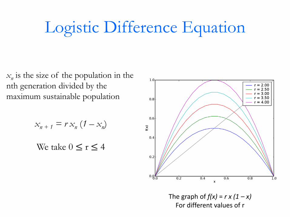
Logistic Difference Equation
xn is the size of the population in the
nth generation divided by the
maximum sustainable population
xn + 1 = r xn (1 – xn)
We take 0 ≤ r ≤ 4
The graph of f(x) = r x (1 – x) For different values of r

Logistic equation with r = 2 and
starting at 0.1
The equation is:
xn + 1 = 2xn (1 – xn)
When x1 = 0.1 then x2 = 2 × 0.1 × (1 – 0.1)
= 0.18
When x2 = 0.18 then x3 = 2 × 0.18 × (1 – 0.18)
= 0.2952
When x3 = 0.2952 then x4 = 2 × 0.2952 × (1 – 0.2952)
= 0.4161
x4 = 0.4161 then x5 = 0.4859
x5 = 0.4859 then x6 = 0.4996
x6 = 0.4996 then x7 = 0.4999
x7 = 0.4999 then x8 = 0.5
x8 = 0.5 then x9 = 0.5
0
0.1
0.2
0.3
0.4
0.5
0.6
0.7
0.8
0.9
1
0 20 40 60 80
Po
pu
lati
on
val
ue
Generation
Logistic Equation with r = 2 Staring at 0.1
Values
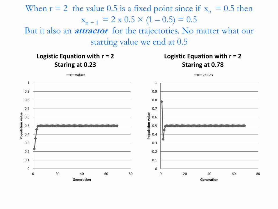
When r = 2 the value 0.5 is a fixed point since if xn = 0.5 then
xn + 1 = 2 x 0.5 × (1 – 0.5) = 0.5
But it also an attractor for the trajectories. No matter what our
starting value we end at 0.5
0
0.1
0.2
0.3
0.4
0.5
0.6
0.7
0.8
0.9
1
0 20 40 60 80
Po
pu
lati
on
val
ue
Generation
Logistic Equation with r = 2 Staring at 0.23
Values
0
0.1
0.2
0.3
0.4
0.5
0.6
0.7
0.8
0.9
1
0 20 40 60 80
Po
pu
lati
on
val
ue
Generation
Logistic Equation with r = 2 Staring at 0.78
Values

Cobweb construction
r = 2.8 start is 0.07

When r = 2.5 then 0.6 is the attractor.
If xn = 0.6 then xn + 1 = 2.5 × 0.6 × (1 – 0.6) = 0.6
0
0.1
0.2
0.3
0.4
0.5
0.6
0.7
0.8
0.9
1
0 20 40 60 80
Po
pu
lati
on
val
ue
Generation
Logistic Equation with r = 2.5 Staring at 0.78
Values
0
0.1
0.2
0.3
0.4
0.5
0.6
0.7
0.8
0.9
1
0 20 40 60 80
Po
pu
lati
on
val
ue
Generation
Logistic Equation with r = 2.5 Staring at 0.23
Values

When r = 3.0
the attractor is now a pair of values and the system oscillates
between them.
0
0.1
0.2
0.3
0.4
0.5
0.6
0.7
0.8
0.9
1
0 20 40 60 80
Po
pu
lati
on
val
ue
Generation
Logistic Equation with r = 3.0 Staring at 0.23
Values
0
0.1
0.2
0.3
0.4
0.5
0.6
0.7
0.8
0.9
1
0 20 40 60 80
Po
pu
lati
on
val
ue
Generation
Logistic Equation with r = 3.0 Staring at 0.78
Values

When r = 3.5
the attractor is now a set of four values and the system oscillates
between them.
0
0.1
0.2
0.3
0.4
0.5
0.6
0.7
0.8
0.9
1
0 20 40 60 80
Po
pu
lati
on
val
ue
Generation
Logistic Equation with r = 3.5 Staring at 0.23
Values
0
0.1
0.2
0.3
0.4
0.5
0.6
0.7
0.8
0.9
1
0 20 40 60 80
Po
pu
lati
on
val
ue
Generation
Logistic Equation with r = 3.0 Staring at 0.78
Values
Going from order to chaos
For r from 0 to 3 there is a point attractor.
For r from 3 to 1 + 6 = 3.449 the attractor is
of period 2
For r slightly above that the period doubles and
the attractor is of period 4.
As r increases period doubling 8, 16, 32 … occurs at
ever more closely spaced values of r until at r =
3.57 the system is no longer periodic – it is
called chaotic.

The system is no longer periodic
it is chaotic
0
0.1
0.2
0.3
0.4
0.5
0.6
0.7
0.8
0.9
1
0 20 40 60 80
Po
pu
lati
on
val
ue
Generation
Logistic Equation with r = 4.0 Staring at 0.78
Values
0
0.1
0.2
0.3
0.4
0.5
0.6
0.7
0.8
0.9
1
0 20 40 60 80
Po
pu
lati
on
val
ue
Generation
Logistic Equation with r = 3.57 Staring at 0.78
Values

Period doubling road to chaos

Period three implies chaos
0
0.1
0.2
0.3
0.4
0.5
0.6
0.7
0.8
0.9
1
0 10 20 30 40 50 60 70 80
Po
pu
lati
on
val
ue
Generation
Logistic Equation with r = 3.8284 Staring at 0.78
Values

Sensitivity to initial conditions
-1
-0.8
-0.6
-0.4
-0.2
0
0.2
0.4
0.6
0.8
1
0 5 10 15 20 25 30 35 40 45 50 55 60 65 70 75 80 85 90 95 100 105
Po
pu
lati
on
val
ue
Generation
Logistic Equation with r = 3.7 Difference between a start at 0.25 with a start at 0.251

Sensitivity to initial conditions
-1
-0.8
-0.6
-0.4
-0.2
0
0.2
0.4
0.6
0.8
1
0 5 10 15 20 25 30 35 40 45 50 55 60 65 70 75 80 85 90 95 100 105
Po
pu
lati
on
val
ue
Generation
Logistic Equation with r = 3.7 Difference between a start at 0.25 with a start at 0.2501
Sensitivity to initial conditions
-1
-0.8
-0.6
-0.4
-0.2
0
0.2
0.4
0.6
0.8
1
0 5 10 15 20 25 30 35 40 45 50 55 60 65 70 75 80 85 90 95 100 105
Po
pu
lati
on
val
ue
Generation
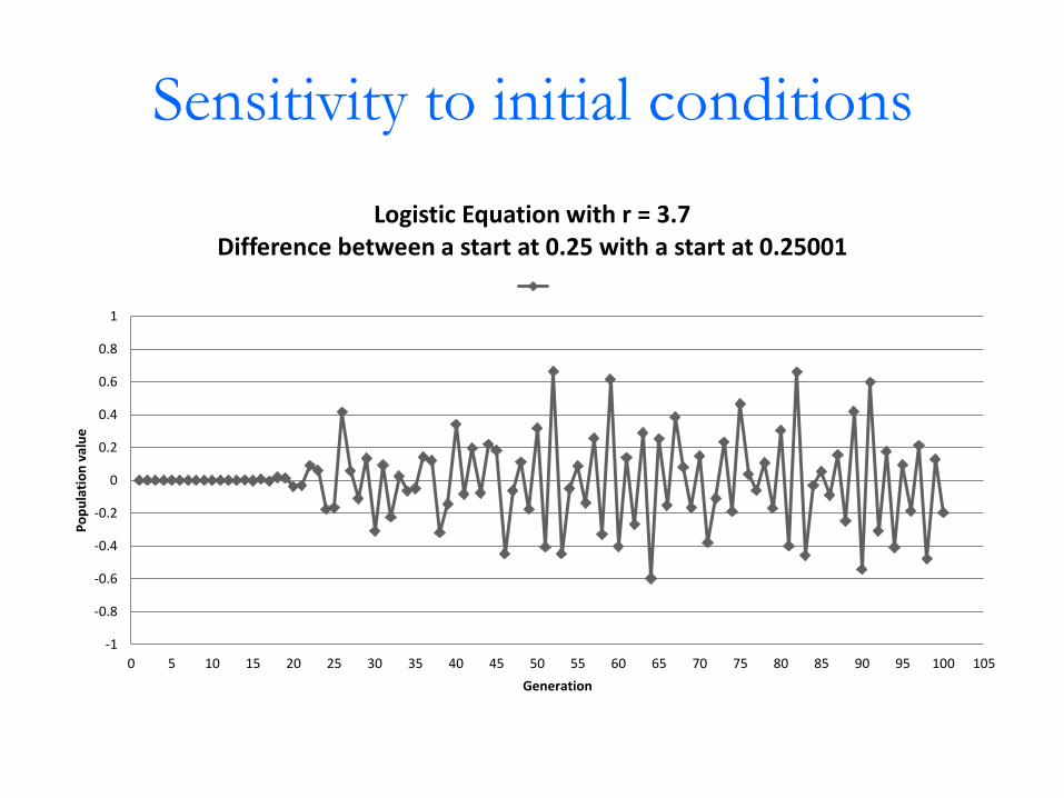
Logistic Equation with r = 3.7 Difference between a start at 0.25 with a start at 0.25001

Sensitivity to initial conditions
-1
-0.8
-0.6
-0.4
-0.2
0
0.2
0.4
0.6
0.8
1
0 5 10 15 20 25 30 35 40 45 50 55 60 65 70 75 80 85 90 95 100 105
Po
pu
lati
on
val
ue
Generation
Logistic Equation with r = 3.7 Difference between a start at 0.25 with a start at 0.250001

Sensitivity to initial conditions
-1
-0.8
-0.6
-0.4
-0.2
0
0.2
0.4
0.6
0.8
1
0 5 10 15 20 25 30 35 40 45 50 55 60 65 70 75 80 85 90 95 100 105
Po
pu
lati
on
val
ue
Generation
Logistic Equation with r = 3.7 Difference between a start at 0.25 with a start at 0.2500001

Sensitivity to initial conditions
-1
-0.8
-0.6
-0.4
-0.2
0
0.2
0.4
0.6
0.8
1
0 5 10 15 20 25 30 35 40 45 50 55 60 65 70 75 80 85 90 95 100 105
Po
pu
lati
on
val
ue
Generation
Logistic Equation with r = 3.7 Difference between a start at 0.25 with a start at 0.25000001
Sensitivity to initial conditions
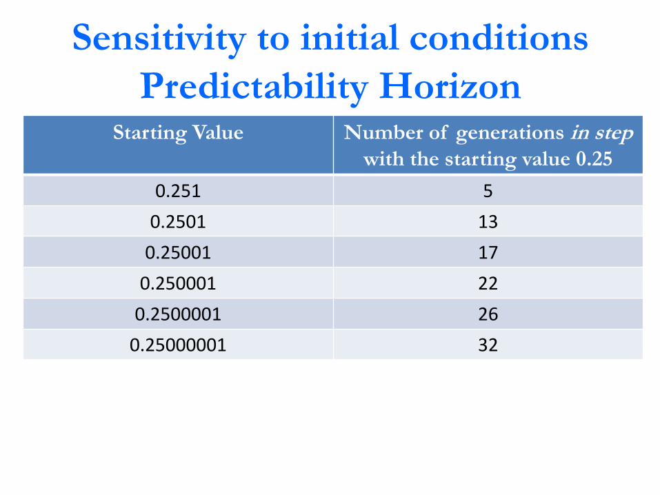
Predictability Horizon Starting Value Number of generations in step
with the starting value 0.25
0.251 5
0.2501 13
0.25001 17
0.250001 22
0.2500001 26
0.25000001 32

Sensitivity to initial conditions
Predictability Horizon Starting Value Number of generations in step
with the starting value 0.25
0.251 5
0.2501 13
0.25001 17
0.250001 22
0.2500001 26
0.25000001 32
TEN fold increase in accuracy of starting values
only gives
LINEAR increase in agreement of population sizes
From this we can estimate the Lyapunov exponent which is a measure of the
average speed with which infinitesimally close states separate

Simple mathematical models with very complicated
dynamics
Robert M. May, Nature, 1976
Not only in research, but in the world of politics and economics, we would all be better off if more people realised that simple non-linear systems do not necessarily possess simple dynamical properties.

Lorenz system Three variables x, y, and z
Three parameters , and β
Edward Lorenz 1917 - 2008

Lorenz Attractor
= 10, = 28 and β = 8/3

Source: http://www.ylilammi.com/lorenzattractor.shtml

Mandelbrot set

Complex numbers
Representing, adding and multiplying

Hopping
• Pick a point, c, on the plane.
• Start at the point c
• Hop according to the rule
The point you are at The point to move to Square the
point you are
at and add c
If you hop off to infinity
colour the staring point c white
otherwise
colour it black
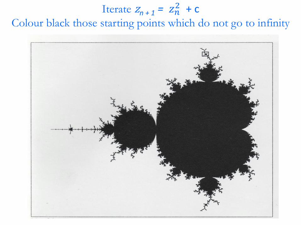
Iterate zn + 1 = 𝑧𝑛2 + c
Colour black those starting points which do not go to infinity

Peitgen and Richter The Beauty of Fractals

Peitgen and Richter The Beauty of Fractals

Peitgen and Richter The Beauty of Fractals

Colours indicate how quickly the point goes to infinity

Zooming in!

Abstract: Geographical curves are so involved in
their detail that their lengths are often infinite or,
rather, undefinable. However, many are statistically
"self-similar," meaning that each portion can be
considered a reduced-scale image of the whole. In
that case, the degree of complication can be
described by a quantity D that has many properties
of a "dimension," though it is fractional; that is, it
exceeds the value unity associated with the
ordinary, rectifiable, curves.
Benoît Mandelbrot: How Long Is the Coast of Britain?
Statistical Self-Similarity and Fractional Dimension Source: Science, New Series, Vol. 156, No. 3775 (May 5, 1967), pp. 636-638

Characterizing the dimension of a
straight line
If you measure a straight line by laying rulers along
it then if you halve the length of the rulers you use
you will need twice as many of them.
We use this scaling to arrive at the dimension of the
line as 1.

How many rulers needed for Britain?
If ruler is of length 200km need 11.5 of them = 2300 km
If ruler is of length 100km need 28 of them = 2800km
If ruler is of length 50km need 70 of them = 3500 km
As the length of the measuring stick is scaled smaller and smaller, the total
length of the coastline measured increases and the number of rulers needed
is increasing by more than a factor of 2

Mandelbrot took the fract in fraction as the root of
the word fractal.
A fractal has fractional dimension
• Construction of Koch curve
• Continue this ad infinitum
• The dimension is ln 4/ln 3 1.26

1 pm on Tuesdays at the Museum of
London Butterflies, Chaos and Fractals
Tuesday 17 September 2013
Public Key Cryptography: Secrecy in Public
Tuesday 22 October 2013
Symmetries and Groups
Tuesday 19 November 2013
Surfaces and Topology
Tuesday 21 January 2014
Probability and its Limits
Tuesday 18 February 2014
Modelling the Spread of Infectious Diseases
Tuesday 18 March 2014