14 TRANSPORTATION RESEARCH RECORD 1338

Bus Route 0-D Matrix Generation: Relationship Between Biproportional and Recursive Methods

PETER G. FURTH AND DAVID s. NAVICK

Planners must sometimes synthesize transit route origin­destination (0-D) matrices with limited data , usually on-off counts and sometimes a small or outdated 0 -D survey sample. When a small 0-D sample is available, iterative methods such as the bi­proportional method that begin with the sample as a seed matrix can be used adjusted to match on-off totals. When only on-off totals are available, the recur ive method ofTsygaJnitsl..J' ha been found to matcb 0-D patterns on some routes better than others. This method is in fact a special ca e of the biproportional method using an implicit null seed matrix that contain information on directionality and minimum trip length. [t illustrates why the recursive method is inappropriate when there is significant com­petition between routes, and offers a correction for when on-off data have been aggregated to the segment level. Estimation errors are then compared to help indicate how large the seed sample should be in order to produce a more accurate estimate than an estimate produced with a null seed.

A route-level origin-destination (0-D) matrix (trip table::) gives the number of passengers traveling between each pair of stops or stations on a transit route in a particular direction. It can be specific to any period of interest, from the individual ve­hicle trip to an entire day. A route-level 0-D matrix is an important descriptor of passenger demand that has been used for such analyses as systematic route evaluations {1,2), route and schedule design for short-turning (3), zonal service ( 4), limited-stop service (5), and complementary express and local service (6).

A route-level 0-D matrix can be obtained by directly sam­pling passengers. The typical passenger survey, in which pas­sengers fill in a questionnaire asking where they boarded and where they plan to leave, leaves a lot to be desired. Response rates are often low, and vary according to critical factors such as trip length-did the passenger have enough time to fill out the questionnaire?-and origin-stop-did the passenger get a seat? Is this stop in a low literacy neighborhood?-which may bias the results. A special purpose survey method, called by one author the "no questions asked" method (2), appears to overcome this nonresponse problem. Passengers are given origin-coded cards when they board and are asked to return the cards when they alight. By careful collection of the cards by alighting stop, 0-D information is obtained. Practitioners report response rates of over 90 percent (2 ,7). However, this method is not in common use, because it requires one checker at each door and careful pre-trip preparation.

Far more common and easier to obtain than 0-D data are on-off counts. In the context of 0-D matrix generation, on-

Department of Civil Engineering, Northeastern University, 360 Huntington Ave., Boston, Mass. 02115.

off counts represent row and column totals. It is not difficult for a ride checker to obtain a 100 percent sample of on-off counts, and measurement error is generally agreed to be quite small. Therefore an 0-D matrix whose row and column totals agree with the on-off counts should be preferred to one ob­tained by simple expansion of a small 0-D sample. Of course, there are many possible 0-D matrices whose row and column totals match the on-off counts. The problem of 0-D matrix synthesis is to generate an 0-D matrix that agrees with a given set of row and column totals and that meets some criteria of being the best or most likely 0-D matrix. Ben-Akiva et al. (8) describe three methods for combining a small 0-D sample with on-off counts: the biproportional method, con­strained maximum likelihood, and constrained generalized least squares. All three of these methods involve iterative computations. The first two are preferable because the third sometimes generates negative m:1trix entries, even though all three yield very similar results. The biproportional method is computationally more attractive, is better known, and has been used in a variety of contexts (9-11). In further work, Ben-Akiva (12) shows how the maximum likelihood approach can be used to derive estimation methods that combine var­ious imperfect sources of information. In an application to transit route 0-D estimation, his assumptions about the struc­ture of the nonresponse bias lead again to the simple bipro­portional method.

It is often the case, however, that a small 0-D sample is not available, or that the small sample is so small or suspected of bias that an estimate based on it may not be reliable. A method for synthesizing a route-level 0-D matrix from on­off counts alone was proposed by Tsygalnitsky {13). It is a very simple method involving a single pass of recursive cal­culations, and can be done by hand (although use of a spread­sheet or computer program is still advi able). This method has also been used by London Transport in at least one study, presumably having been developed independently (J). Tsy­ga!nil~ky found that his recursive method fit well with data from Toulouse, France. Simon and Furth (7) also tested it against 0-D data from two routes in Los Angeles, and again found a good fit, although the fit on one route was better than that on another. Ben-Akiva et al. (8) tested the recursive method against 0-D matrices generated using the bipropor­tional and constrained maximum likelihood methods for two Boston area routes and found that it yielded matrix estimates that differed substantially from the estimates obtained by the iterative methods based on a small-sample 0-D survey.

Although Tsygalnitsky's recursive method and the bipro­portional method are motivated from different assumptions,

Furth and Navick

the recursive method is actually a special case of the bipro­portional method. The biproportional method takes an initial matrix, called a seed matrix, and factors it to match on-off counts . The seed matrix contains information concerning the preferences for the various 0-D pairs. Typically, the seed matrix is an 0-D sample. If there is no 0-D sample to begin with, a reasonable guess is to use a "null seed," one that assumes that every permissible 0-D pair is equally preferred. It is demonstrated that Tsygalnitsky's recursive method is the same as the biproportional method using a null seed.

This insight makes it possible to better analyze which method is more appropriate under various circumstances. A small 0-D sample contains valuable site-specific information about 0-D pair preferences but is also subject to sampling error and nonresponse bias. A null seed has no sampling error or nonresponse bias but lacks site-specific information. In ad­dition, two common factors-aggregation of stops into seg­ments and competition from other routes-are shown to be in contradiction to the assumptions underlying the null seed, and consequently the recursive method should not be ex­pected to perform well under these circumstances.

BUS ROUTES ANALYZED

Repeated reference is made to four bus routes that have been previously analyzed. Lines 16 and 93, analyzed by Simon and Furth (7) are operated by the Southern California Rapid Tran­sit District. For Line 16, virtually complete 0-D data, en­compassing 266 passengers, were obtained from five inbound short-turning trips over a 5-mi radial route containing 40 stops. For Line 93, virtually complete 0-D data were obtained on four a.m.-peak (383 passengers) and four p.m.-peak (273 pas­sengers) trips. Four trips were local trips covering the entire 140-stop route from downtown Los Angeles to the San Fer­nando Valley, three trips were short-turned in North Holly­wood (about 90 stops), and one p.m. trip ran express from downtown to the valley. Routes 77 and 350, analyzed by Ben Akiva et al. (8), are operated by the Massachusetts Bay Trans­portation Authority. These routes were analyzed inbound in the a.m. peak and outbound in the p.m. peak . The available data consist of a small 0-D sample augmented by on-off counts. Route 77 is a heavily used radial route, 5.5 mi long, running through the suburb of Arlington into Harvard Square in Cam­bridge. In the a.m. peak, 2,148 passengers were counted, and 0-D data were obtained from 54. In the p.m. peak, 1,617 passengers were counted, with 0-D data obtained from 138. Route 350 is 15.2 mi long, with a large collection/distribution section in suburbs north of Boston, connected by express operation to selected stops in Cambridge and downtown Bos­ton. In the a.m. peak, 485 passengers were counted, with 0-D data obtained from 76. In the p .m. peak, 200 passengers were counted, with 0-D data obtained from 61.

TSYGALNITSKY'S RECURSIVE METHOD

Tsygalnitsky's recursive method proceeds stop by stop, dis­tributing alightings at each stop among origin stops in pro­portion to the number of people from each origin stop who are eligible to alight. To be eligible, passengers must have

15

traveled a minimum distance, and must not have alighted previously. Taking each stop as a node, with nodes consec­utively numbered from 1 to n in the direction of travel, let

t;1 = passenger trips from i to j, t;. = boardings at i = "i};1,

t.1 = alightings at j = I;t;1,

m; first node at which passengers who board at i are eligible to alight (m; ~ i),

E1 set of nodes that can serve as origins for passengers alighting at j,

e;1 = number of passengers who boarded at i who are eli­gible to alight at j,

e.1 = total number of passengers eligible to alight at j I,e;1, and

fj = fraction of eligible passengers who alight at j t) e.1

Initially, set e;1 = 0 for all (i, j) except when j = m;, in which case set e;1 = t;. · Computation begins with the first node at which passengers are eligible to alight; call it Node k. After calculating e.k and fk> let

(1)

Stop if k = n; otherwise update:

(2)

and advance to the next node (let k = k + 1) and return to Equation 1.

Simon and Furth call this method a fluid analogy, because passengers on the bus are likened to a thoroughly-mixed fluid out of which alighting passengers are drawn at each alighting stop in proportion to their representation in the fluid . Newly boarding passengers are added to the fluid after they have met the minimum travel distance criterion. (This minimum distance may be expressed in stops, distance, or time units, and may vary from stop to stop.) Ben-Akiva et al. (8) call it an intervening opportunities method, because it follows the logic of classical intervening opportunities models in giving priority to closer destinations.

BIPROPORTIONAL METHOD

Additional notation that will be used is

S;k = seed matrix, A; = overall adjustment factor for row i, Bk = overall adjustment factor for column k.

The seed matrix contains information about relative like­lihoods of 0-D pairs to be chosen by travelers. It may be a small-sample 0-D matrix or an out-of-date 0-D matrix. If no empirical seed matrix is available , a seed matrix can be created by an analyst to reflect information available on preferences between 0-D pairs, as done by Furth (14) for vehicular traffic at an intersection.

The method is to alternately balance rows and columns to match the desired row and column totals until convergence. Initially, we set t;k = s;k· Then, for iteration h, rows are balanced:

for all rows i (3)

16

where the balancing factor a7 is the ratio of the desired row i total to the current row i total. Next, columns are likewise balanced:

for all columns k (4)

where the balancing factor bZ is the ratio of the desired column k total to the current column k total. Since balancing columns upsets the balance of the rows, the process is repeated until convergence is reached, that is, until, after balancing the col­umns, all the row totals agree (to some arbitrary tolerance) with the desired row totals. Reflecting the logic of the cal­culations, one name that has been used for this method is "iterative proportional fit." The name "bi proportional method" derives from the form of the final estimate for cell (i, k), which is

(5)

where the overall balancing factor for row i is A, = Tiha7 and the overall balancing factor for column k is Bk = TihbZ. It is well known that the biproportional method has a unique so­lution (15,16). In general, there is no closed form or single­pass recursive algorithm for determining the overall balancing factors, which must therefore be found by an iterative method such as the iterative proportional fit.

The biproportional method has been derived in several dif­ferent ways. Several authors, including Ben-Akiva et al. (8) and Lamond and Stewart (16), derive it as a case of minimizing a measure of discrepancy between the estimate and the seed. Hauer et al. (JO) derive it as the moi;t lihly rn;iliwtion of o random (either Poisson or multinomial) process in which the seed represents the known ocurrence rates. Ben-Akiva (12) derives it as the maximum likelihood estimate of the popu­lation trip rates, assuming that the seed is a random sample subject to sampling bias, and the relative bias is a product of two factors, one from the origin stop and one from the des­tination stop.

RECURSIVE METHOD AS SPECIAL CASE OF BIPROPORTIONAL METHOD

The estimates produced by Tsygalnitsky's recursive method are actually a biproportional form. Implicitly underlying the recursive model is a null seed containing information on whether travel is permitted or not, based on directionality and mini­mum trip length, given by

if travel from i to k is permitted otherwise (6)

The recursive method also implies the following restrictions on the seed: s1" = 1 for all i, and for all k < n, s1.k+ 1 = 1 if S;k = 1.

Theorem

The recursive method is a special case of the biproportional method in which the seed matrix is the null seed matrix given

TRANSPORTATION RESEARCH RECORD 1338

by Equation 6. More specifically, the recursive estimates t1k = e,Jk (Equation 1) are equivalent to the biproportional estimates t1k = s1kA1Bk (Equation 5), where

for all i = 1, . . . , n (7)

(8)

and

for all k = 1, . . . , n - 1 (9)

Proof (by construction)

Because the biproportional method has a unique solution, it is sufficient to prove that estimates produced by the recursive method have a biproportional form. Consider column n (i.e., let k = n). By inspection, it is clear that Equations 1 and 5 are equivalent. Now consider column n - 1 (i.e., let k =

n - 1). By construction, the recursive method yields e1.n = ei.n - i (1 - fn _ 1) if travel from i to n - 1 is permitted. Rear­ranging, we obtain

if travel from i ton - 1 is permitted (10)

otherwise

Substituting for e1,,,_ 1 yields

(11)

which is a biproprotional form with the balancing factors given by Equations 7 and 9.

Now consider column n - 2 (i.e., k = n - 2). By similar argument,

iftravelfromiton - 2ispermitted (12)

otherwise

Combining Equations 11 and 12 yields

ei,n - 2 =

if travel from i ton - 2 is permitted

otherwise (13)

Substituting for e1.n _ 2 in Equation 1 with k = n - 2 again yields a biproportional form, with balancing factors given by Equations 7 and 9. Similar reasoning can be applied to each successive column k = n - 3, n - 4, ... Equation 13 becomes generalized to

if travel from i to k is permitted

otherwise (14)

Furth and Navick

from which the equivalence of Equations 1 and 5, using the substitutions given by Equations 7 and 9, is obvious. Q. E. D.

This theorem provides a framework for determining which method of transit route 0-D matrix generation, the recursive or biproportional method, is better. Because the two methods differ only in which seed is used, the question can be reframed in terms of which seed is better, a null seed or a seed derived from exogenous data such as a small sample. We have already mentioned a few empirical studies of the methods. The re­mainder of this paper examines theoretical deficiencies of both the null seed and the small sample seed in common situations along with some experimentation, offering further guidance as to which seed is most appropriate in various situations.

One interesting corollary of this theorem is that when the seed has the form of a null seed, the recursive method provides a single-pass algorithm for finding the bi proportional solution. Another corollary is that the recursive method is reversible; that is, it will yield the same results if one works backward or forward along the route. In this sense, the recursive method is not myopic like other intervening opportunities models. It appears to be myopic since it determines demand to stops along the route without explicitly considering what oppor­tunities lie further downstream.

FACTORS AFFECTING APPLICABILITY OF RECURSIVE METHOD

The fact that the recursive method is the same as the bipro­portional method with a null seed helps indicate the types of routes and situations in which the recursive model can or cannot be expected to perform well. It can be expected to perform well when there is little a priori reason to believe that anything other than the popularity of the origin and des­tination stops is responsible for the demand for travel between 0-D pairs. In the two situations suggested by Tsygalnitsky (13), a null seed appears plausible. These situations are (a) an express route with a collection segment outside the city and a distribution segment downtown, with travel permitted only between the collection and distribution segment; and (b) a short local route free from interference (e.g., competition) with other routes.

However, there are other situations in which a null seed violates a priori knowledge of trip-making behavior, the fore­most being when significant competition from other routes affects demand. For example, imagine a local route between Segment A and Segment E, with several intermediate seg­ments . If there is another route that goes express from Seg­ment A to Segment E, we would expect that the express route would capture most of the demand from A to E. The seed matrix for the local route should therefore have a relatively low propensity for stop pairs that are served by the express route, rather than equal propensities throughout. Likewise, if two local routes begin at a common intersection uptown and end at a common location downtown and use different paths to get there, the travel market that can use either route will be split between the routes , lowering on both routes the propensity to travel between stop pairs served by both routes. Other network effects can affect travel propensity along a route as well. For example, a large transfer volume from a

17

feeder route can influence propensity for travel between that transfer point and other stops on the main route because these transferring passengers may have a high propensity to go to certain portions of the main route, but not to other portions (e.g., there may be a more expedient path to some portions of the main route than via that transfer point).

Long local routes may be another example of the unsuit­ability of a null seed. Travel propensity is commonly agreed to decline with distance, except for very short distances, where competition with walking yields the opposite effect. On short routes , travel time differences between different 0-D pairs are sufficiently minor that an equal-propensity seed is still plausible. But on long routes, even if there is no competition from other routes, propensities should be expected to be smaller for long trips than for short trips . It has yet to be shown how long a route can be before the null seed assumption becomes unrealistic.

Results reported in the literature confirm these expecta­tions. For example, Tsygalnitsky found that his method per­formed very well on the two routes he tested, one an express route with separate collection and distribution areas, the other a short local route . Simon and Furth (7) found that Tsygal­nitsky's recursive method worked very well on a short local route, but that on a longer route with competition from ex­press routes, it overpredicted very long trips. It should be noted that, because the average trip length is determined by the given on and off totals on the route, any model for 0-D matrix generation must yield the correct average trip length. Therefore, an overprediction of long trips must be accom­panied by an overprediction of short trips. Ben-Akiva et al. found that the recursive method overpredicts very long and very short trips, particularly on Route 350, a long route with competition from express service . It is not clear, however, whether the discrepancies on these longer routes arise because of interference from competing routes, from route length, or from using segment-level data.

0-D MATRIX ESTIMATION WITH SEGMENT-LEVEL DATA

An important factor affecting the applicability of the recursive method is whether the on-off counts are by individual stop or by segment (aggregations of stops). With stop-level data , travel along the diagonal of the 0-D matrix (i.e., beginning and ending at the same stop) is not permissible , but with segment-level data, travel along the diagonal is permissible. Although the recursive method recognizes only the dichotomy permissible/not permissible (1 or 0), the possibility of intra­segment travel calls for a finer level of gradation. Intraseg­ment travel in a segment with n stops is an aggregation of n2

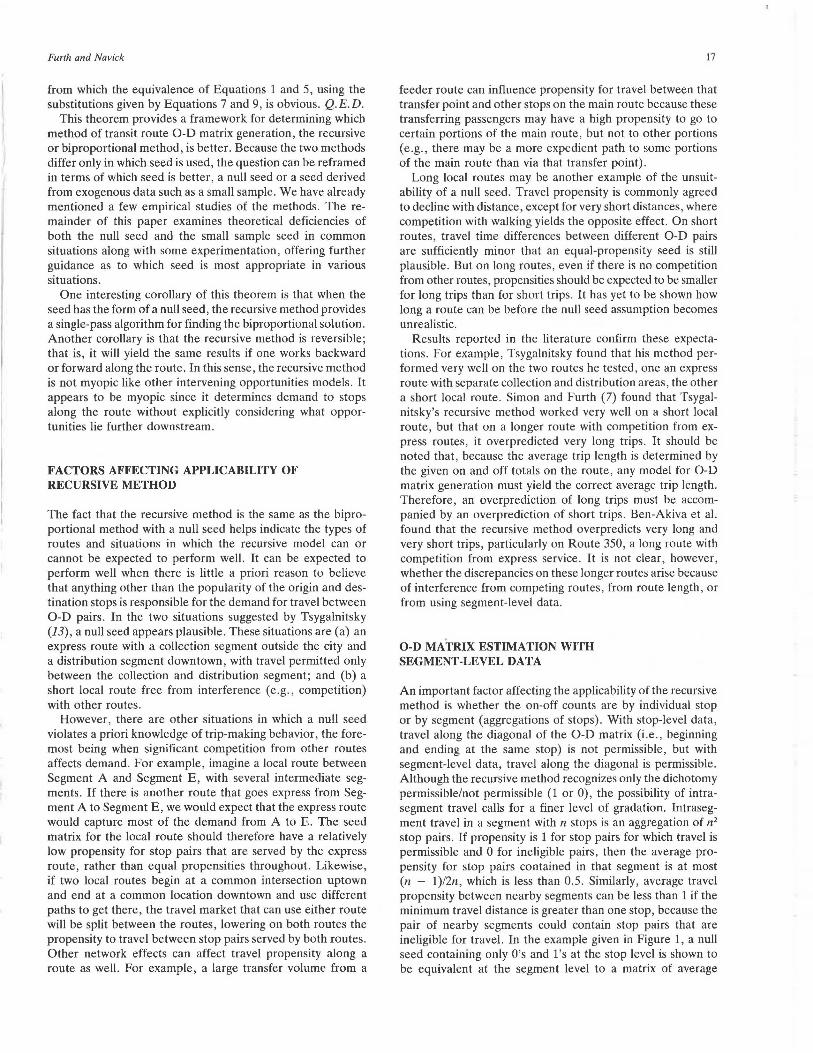
stop pairs. If propensity is 1 for stop pairs for which travel is permissible and 0 for ineligible pairs, then the average pro­pensity for stop pairs contained in that segment is at most (n - 1)/2n, which is less than 0.5. Similarly, average travel propensity between nearby segments can be less than 1 if the minimum travel distance is greater than one stop, because the pair of nearby segments could contain stop pairs that are ineligible for travel. In the example given in Figure 1, a null seed containing only O's and l's at the stop level is shown to be equivalent at the segment level to a matrix of average

18

~ Froru I 2

I n 2 0 3 0

A 4 0 s 0 6 0

8 7 0 0

8 0 0 9 0 n

c 10 0 0 11 0 0

D 12 0 0

a. Stop-Level Propensity (Minimum travel distance• ) slOps)

A. 8 3 4 , 6 7 8 9

I I T T I I 0 I I 1 I I 0 0 I I I I

0 n I 1 1

0 0 0 I I 0 0 0 0 I

0 0 0 n 0 0 0 0 0 0 0 0 0 0 0 0 0 0 0 0 0 0 n 0 0 0 0 0 0 0 lf 0 0

0 0 0 0 0 0 0

c D tu 11 12

I I I I I I I I I I I I I I I I I

I I I 0 I I 0 0 I II u u u u u 0 0 0

b. Sesment-Level Eqw·valent, Showing Average Propensities

~ A. 8 c D Froru 1121314f516 7 8 I 9 I tu I 11 12

1

2 3 6/36 4/6 23 /24 A 4 I 5 6

B 7 n n "7/J. I

8 9

0 0 I /16 2/4 c 10 11

D 12 0 0 0 u

FIGURE 1 Stop-level null seed and segment­level equivalent.

propensities that include, besides O's and l's, fractional values ranging from 1/16 to 23/24.

__ Because the recursive algorithm itself does not-permit.frac­tional propensities, applying it to segment-level data will bias results, because this method forces all those fractional pro­pensities to be l's. For example, Ben-Akiva et al. apply the recursive method to segment-level data, setting the minimum travel distance to zero in order to make intrasegment travel permissible. As should be expected, they find that the method predicts too many intrasegment trips. In contrast, Simon and Furth (7) and Tsygalnitsky apply the recursive method at the stop level, although the results are often presented at the segment level, avoiding this bias. This effect no doubt ac­counts in part for the poor fit found by Ben-Akiva et al. using the recursive method.

When only segment-level data are available, a method of synthesizing 0-D matrices that is consistent with the recursive method at the stop level is the biproportional method with a seed matrix consisting of segment-level average propensities. An example using data from Line 93 demonstrates how using this "equivalent null seed" avoids the large bias of a naive segment-level application of the recursive method. Table 1 shuws fuui sels uf resulls (pn:sented at the segment level even if the analysis was done at the stop level): (a) the actual 0-D matrix; (b) the stop-level estimate using a stop-level null seed (minimum trip length = 2 stops), which is the same as a recursive estimate; (c) the segment-level estimate made using the segment-level equivalent null seed; and (d) the segment-level estimate made using a naive null seed (mini­mum trip length = 0 segments), which is the same as a re­cursive estimate made at the segment level. Three different error measures are used: relative root-mean-square error (RRMSE), root-mean-weighted fractional error (RMWFE),

TRANSPORTATION RESEARCH RECORD 1338

and x2. The RMWFE can be used to judge whether the actual data obtained agree with the model. Formulas for these mea­sures applied at the segment level are

RMWFE = {_!_ i i [(i11 - t,1)2]}112 t .. • ~ 1 1 ~ · 1,,

where

~i = passenger trips from i to j, tii = synthesized passenger trips from i to j, t .. = total passenger trips, and

(15)

(16)

(17)

K = number of matrix cells containing permissible trips.

The segment-level estimate made using the equivalent null seed is almost as good as the stop-level estimate. The equiv­alent null seed minimizes aggregation bias, and aggregation error, as shown by the increase in the error measures, is small. The results are markedly worse when the recursive algorithm is applied naively at the segment level. The tendency in this case to predict too many very short and very long trips is clearly seen. The same analysis was performed for Line 16 and similar results were obtained.

An attempt was also made to assess the effect of aggregation bias_ on the_ t~sts performed _by Ben~Aiciv_a et al. (8). Thrt<t< segment-level estimates for Route 77 outbound are shown in Table 2: the "best" estimate, a biproportional estimate gen­erated using a small-sample 0-D survey as a seed; the estimate using an equivalent null seed based on a minimum trip length of three stops; and the naive estimate using a segment-level null seed (minimum trip length = 0 segments). Because stop­level data were not available, it was impossible to generate a stop-level estimate and compare the results with the true dis­tribution. Measures of error are in comparison with the best estimate. The equivalent null seed estimate approximates what would be obtained from a proper stop-level application of the recursive method. The comparison of these cases clearly shows how the naive segment-level application of the recursive method increases the estimated number of very short and very long trips.

SAMPLING ERROR AND BIAS WITH SMALL-SAMPLE SEED

It may seem that any empirical seed, whether from a small­sample 0-D survey or an old 0-D survey, would be superior to pleading ignorance and using a null seed. However, a null seed is not such a bad guess for many situations, being con­sistent with our understanding of travel behavior and having been confirmed on a few test routes. Before an empirical seed is used with the biproportional method or another iterative method, the value of its information content should be con­sidered. Although information content can in many contexts be difficult to judge, in the case of a small-sample 0-D matrix

TABLE 1 COMPARISON OF STOP-LEVEL AND SEGMENT-LEVEL ESTIMATES, LINE 93, a.m.

a. Actual 0-D Matrix

From I To I 2 3 4 7 On l 0 14 9 5 8 7 5 51 2 12 10 12 22 25 7 89 3 3 18 16 2 18 57

3 20 12 3 40 6 25 11 45

8 28 38 32 47

16 22 38 72 79

b. Stop-Level Estimate

From I To I 2 3 4 7 I o.o II . 6.4 7.6 10.3 .3 .s 1.4 I 2 14.4 12.1 13.8 20.0 15.6 10.7 2.4 89 3 3.5 11.8 17.2 12.4 9.4 2.7 51 4 4.8 14.0 12.9 6.9 1.4 40 5 10.5 19.5 12.2 v 45 6 10.3 25.6 2.2 38 7 33.7 13.3 47 8 16.0 16

Off 2 22 38 72 79 104 42 383

c. Segment-Level Esrimate with Equivalent Null Seed

6 7.

15.9 13.0 ll.4 18.9 12.1

d. Segment-Level Estimate with Naive Null Seed

From I To I 2 3

I . ~

16.5 15.6

22 JR 72

12.2 9.9

13.9 18.5

I

1.9 51 3.3 89 2.6 57 2.1 40 2.9 45 3.9 38 9.4 47

16.0 16 42 83

RRMSE = 0.352

RMWFE=0.479

Chi Squared= 47.2

RRMSE = 0.368

RMWFE = 0.513

Chi Squared'= 52.2

RRMSE = 0.534

RMWFE = 0.641

Chi Squared= 94.8

TABLE 2 COMPARISON OF SEGMENT-LEVEL ESTIMATES, ROUTE 77 OUTBOUND

a. Estimate using Small 0-D Sample Seed

From I To 1 2 4 s 6 7 I 0. 14. 16.2 3.2 I . I. 92.4 l 2 6.5 56.7 6.5 13.0 84.3 298. l 465 3 9.7 3.2 1.6 38.9 228.5 282 4 6.5 3.2 4.9 197.7 212 5 o.o 9.7 110.2 120 6 40;5 367.8 408 7 0.0 0

or 0 21 19 19 180 1295 1617

b. Segment-Leve/ Estimate with Equivalent Null Seed

Fro mlTo I 2 3 4 5 6 7 On l o.u 11.8 16.2 2.4 2.1 14.6 SH 130 2 9.2 57.9 9.4 8.0 57.0 323.4 465 3 8.9 6.1 S.5 39.2 222.3 282 RRMSE = 0.197

4 I .I 3.4 31 .1 176.4 212 s o.o, 15.4 '104.6 120 6 22.7 385.3 408

RMWFE = 0.427

7 o.o 0 Chi Squared= 106.3 orr 0 21 83 19 19 180 1295 1617

c. Segment-Level Esrimate with Naive Null Seed

Fro mlTo l l 3 4 s 6 7 On 1 0.0 4.6 12.2 21 1.9 13.3 95.8 130 2 16.4 43.5 7.8 7.0 47.6 342.7 465 3 27.3 4.9 4.4 29.9 215.4 282 RRMSE = 0.242 4 4.1 3.6 24.9 179.3 212 s 2.1 14.4 103.S 120 RMWFE=0.407 6 49.8 358.2 408 7 0.0 0 Chi Squared= 126.1

arr 0 21 83 19 19 (HO 1295 1617

20

seed, the information content can be evaluated in terms of bias and sample size.

The main bias in 0-D surveys is nonresponse bias, which is present if the response rate is substantially below 100 per­cent, a condition endemic to surveys on busy bus routes, and the nonresponding population is different in its 0-D patterns from the responding population. The differences most often cited are as follows : nonresponders (a) are more likely to come from segments of the route in neighborhoods that have lower literacy or are less cooperative, or both ; (b) are more likely to board where the route is crowded and they can't get a seat; and (c) are more likely to be making short trips , leaving them too little time to complete a survey. Fortunately, the first two biases are proportional to the response rates at each origin and each destination stop , and since the biproportional method correctly expands origin and destination totals, these biases disappear, as confirmed by Ben-Akiva (12). The third bias, however, remains, and can be significant, though its extent is hard to judge.

The effect of sample size on quality of information in an 0-D matrix is also well known. A common rule of thumb is that an observation of fewer than five travelers in a cell is unreliable, since a difference of one or two people can effect an enormous relative change in the value. In the extreme case, a cell with no observations poses a special challenge, since a biproportional estimate for a cell must be zero if its seed value is zero. If a small-sample 0-D matrix, aggregated to the segment level , where the segment is the level of the detail one is finally interested in, has a substantial number of cells with fewer than five observations , the information con­tent of the seed may be so compromised by sampling error that it is worse than the information content of a null seed .

For example, the small-sample 0-D surveys used by Ben­Akiva et al. (8) are all quite small, containing 61, 76, 138, and 54 responses for the four route/direction combinations studied . In the case with the greatest sample size, Route 77 outbound, only 8 of 25 segment-to-segment cells contain five or more observations, and six of these all lie in the same column of the matrix alighting at the last stop. Ten of the 25 cells contain no observations at all. An estimate based on such a seed seems risky.

Ben-Akiva et al. respond to the problem posed by cells with zero observations by offering a correction to deal with these "non-structural zeros." Even with this correction, es­timates based on the empirical seed are heavily influenced by patterns that appear in the seed. Their estimate for Route 77 outbound made using this empirical seed (Table 2a , equiva­lent to their Table 3) contains the peculiar pattern in which, although there is substantial demand from Segments 1 to 7 (92 passengers) and from Segments 2 to 6 (84 passengers), there is virtually no demand from Segments 1 to 6 (1.6 pas­sengers), because in the small-sample 0-D survey, no one went from 1 to 6. In contrast, the estimate resulting from the equivalent null seed (Table 2b) has a much more typical pat­tern, assigning a far larger volume (14.6 passengers) to 0-D pair 1- 6. Because Route 77 is a short route and, at the time of data collection, had no significant competition from other routes, a null seed seems quite plausible. The question is whether the peculiar p,attern found using the small-sample seed is a reflection of true patterns in the population, or just the spurious outcome of a random sampling process .

TRANSPORTATION RESEARCH RECORD 1338

The effect of sample size can be addressed more rigorously. Ben-Akiva et al. provide equations for determining the ap­proximate standard error of a biproportional estimate based on the number of observations in a cell, and also report approximate standard errors of their estimates. However, be­cause many of their results are reported normalized to a stan­dard grand total, the level of accuracy attained is not im­mediately apparent. Reversing the normalization, it was found that for the case of Route 77 outbound , the relative standard error of their estimates (standard error divided by estimate) is quite small (below 13 percent) for all six eligible cells in which the destination is Segment 7. These were the cells with many observations in the empirical seed. In the remaining 19 eligible cells of the matrix, the seed contained only 26 ob­servations. Consequently, the relative standard error is greater than 100 percent in a majority of those cells. For the entire matrix, the average passenger volume per eligible cell is 17, and the average approximate standard error is 8.4. With a smaller sample size, as in the other three cases examined by Ben-Akiva et al. (8), errors can be substantially larger.

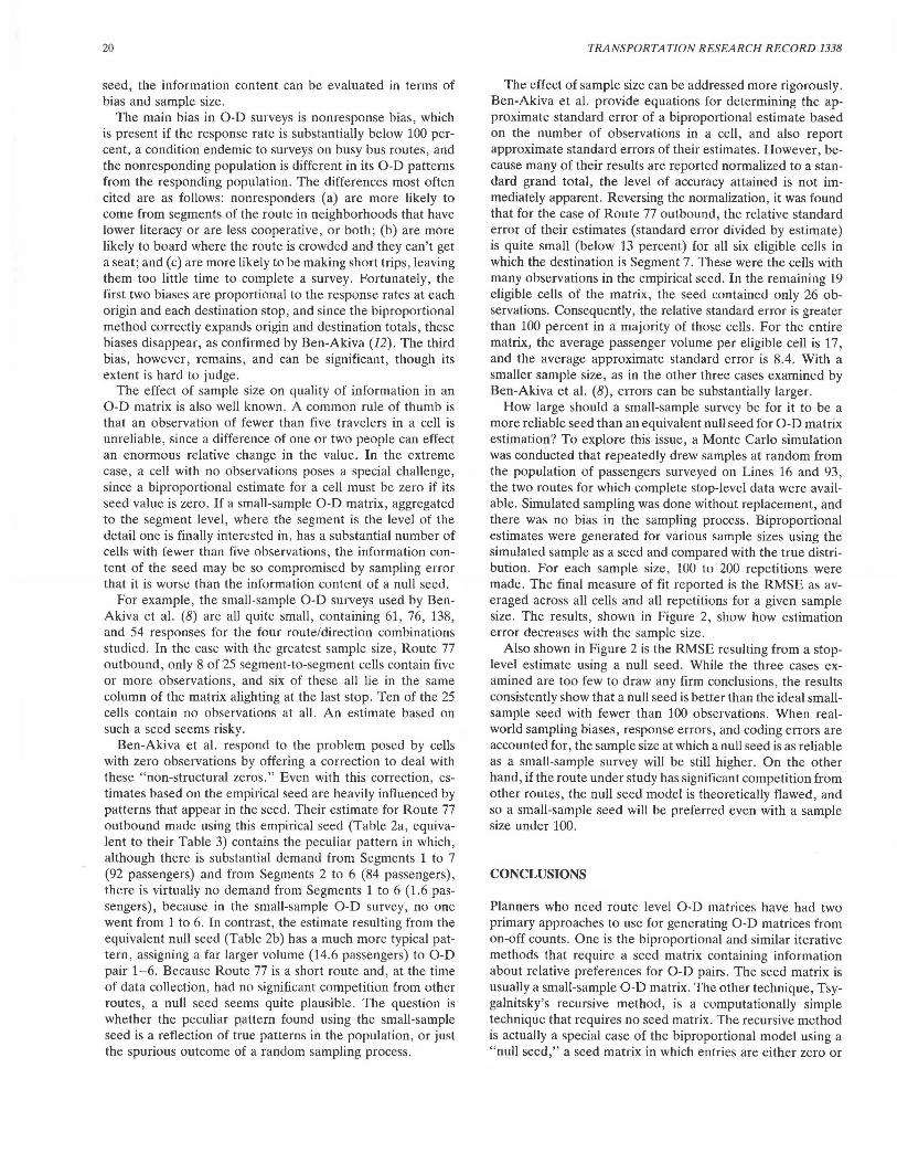
How large should a small-sample survey be for it to be a more reliable seed than an equivalent null seed for 0-D matrix estimation? To explore this issue, a Monte Carlo simulation was conducted that repeatedly drew samples at random from the population of passengers surveyed on Lines 16 and 93, the two routes for which complete stop-level data were avail­able . Simulated sampling was done without replacement, and there was no bias in the sampling process . Biproportional estimates were generated for various sample sizes using the simulated sample as a seed and compared with the true distri­bution. For each sample size, 100 to 200 repetitions were made. The final measure of fit reported is the RMSE as av­eraged across all cells and all repetitions for a given sample size. The results, shown in Figure 2, show how estimation error decreases with the sample size.

Also shown in Figure 2 is the RMSE resulting from a stop­level estimate using a null seed. While the three cases ex­amined are too few to draw any firm conclusions, the results consistently show that a null seed is better than the ideal small­sample seed with fewer than 100 observations. When real­world sampling biases, response errors, and coding errors are accounted for, the sample size at which a null seed is as reliable as a small-sample survey will be still higher. On the other hand, if the route under study has significant competition from other routes, the null seed model is theoretically flawed, and so a small-sample seed will be preferred even with a sample size under 100.

CONCLUSIONS

Planners who need route level 0-D matrices have had two primary approaches to use for generating 0-D matrices from on-off counts. One is the biproportional and similar iterative methods that require a seed matrix containing information about relative preferences for 0-D pairs. The seed matrix is usually a small-sample 0-D matrix. The other technique, Tsy­galnitsky's recursive method, is a computationally simple technique that requires no seed matrix. The recursive method is actually a special case of the biproportional model using a " null seed," a seed matrix in which entries are either zero or

Furth and Navick

12.00

11.00

10.00

9.00

8.00

7.00

RMSE 6.00

S.00

4.00

3.00

2.00

1.00

0.00

20 40 60 80 100 120 140 160 180 200

Sample Size

... Linel6 <>-Line93AM ·•·Line93PM NullSeed N=266 N=383 N=273 (!)

FIGURE 2 Estimation error versus sample size.

one, corresponding to whether travel between stop pairs is permissible based on direction of travel and minimum travel distance. A null seed is theoretically plausible on certain types of routes, such as relatively short routes with little interference (e.g., competition) from other routes. Empirical tests on dif­ferent bus routes confirm this hypothesis.

The structure of the null seed underlying the recursive method implies that it is unsuitable for application to segment-level data. Instead, the biproportional method should be applied using an "equivalent null seed," a seed whose values are the average stop-level null seed propensity averaged over the stop pairs comprehended in a segment-level pair. This method yields results that closely approximate estimates made using the recursive method with stop-level data. It is probably the best method available for generating a transit route 0-D ma­trix from segment-level data when there is no reliable small­sample survey or old 0-D matrix to serve as a seed.

Finally, a comparison of estimation error using an equiv­alent null seed versus using a small 0-D sample seed indicates, at least for the routes tested, that an ideal small-sample survey is preferable to a null seed when the sample size is over 100, and that a null seed is preferable when the sample size is smaller. In real-world applications, modifications to this

21

threshold should be made to account for imperfections in the sampling process and competition between routes.

REFERENCES

1. London Tran port International Consultant· , Inc. Route, Sched­ule and Ridership Analysis. Final Reportffechnical Report to Dallas Area Rapid Transit. May 1987.

2. P. R. Stopher, L. Shillito, D . T. Grober, and H . M. Stopher. On-Board Bus Surveys: No Questions Asked. In Tra11sportatio11 Research Record 1085, TRB, National Research Council, Wash­ington, D .C., 1985, pp. 50-57.

3. P. G. Furth. Short-Turning on Transit Routes. In Transportation Research Record 1108, TRB, National Research Council, Wash­ington, D.C., 1988, pp. 42-52.

4. P. G. Furth . Zonal Route Design for Transit Corridors. Trans­portation Science, Vol. 20, No. 1, 1986, pp. 1-12.

5. P. G. Furth and F. B. Day. Transit Routing and Scheduling Strategies for Heavy Demand Corridors. In Transportation Re­search Record 1011 , TRB, National Research Council, Wash­ington, D.C., 1985, pp. 23-26.

6. P. G. Furth, F. B . Day, and J. P. Attanucci. Operating Strategies for Major Radial Bus Routes. Report DOT-I-84-27. UMTA, U.S. Department of Transportation, 1984.

7. J. Simon and P. G. Furth. Generating a Bus Route 0-D Matrix from On-Off Data. ASCE Journal of Transportation Engineering, Vol. 111 , No . 6, 1985, pp. 583-593 .

8. M. Ben-Akiva, P. Macke, and P. S. Hsu. Alternative Methods to Estimate Route Level Trip Tables and Expand On-Board Surveys. In Trn11sportatio11Research Record 1037, TRB, National Research Council , Washington, D.C., 1985, pp. 1-11.

9. P. G . Furth . Updating Ride Checks with Multiple Point Checks. In Transportation Research Record 1209, TRB, National Re­search Council, Washington , D .C., 1989, pp. 49- 57.

10. E. Hauer, E. Pagil as, and B. T. Shin . Estimation of Turning Flows from Automatic Counts. In Tra11sportatio11 Research Rec­ord 795, TRB, National Research Council, Washington, D.C., 1981, pp. 1-7.

11. M. G. H. Bell. The Estimation of an Origin-Destination Matrix from Traffic Counts. Transportation Science, Vol. 17, No. 2, 1983, pp. 198- 217.

12. M. Ben-Akiva . Methods to Combine Different Data Sources and Estimate Origin-Destination Matrices. In Transportation ai1d Traffic Theory (N. H. Gartner and N. H. M. Wilson, eds. ) Elsevier, 1987.

13. S. Tsygalnitsky. Simplified Methods for Transportation Planning. M.S. thesis, Department of Civil Engineering, Ma sachuseits In­stitute of Technology, Cambridge, 1977.

14. P. G. Furth. Model of Turning Movement Propensity. In Trans­portation Research Record 1287, TRB, National Research Coun­cil, Washington , D.C., 1990, pp. 195- 204.

15. M. Bacharach. Biproportio11al Matrices and Input-Output Change. Cambridge University Press, London, 1970.

16. B. Lamond and N. F. Stewart. Bregman's Balancing Method. Transportation Research, Vol. 15B, No. 4, 1981, pp. 239-248 .

Publication of this paper sponsored by Committee on Bus Transit Systems.