bugles, trumpets, beltrami 190220 - josmfs.net

Bugles, Trumpets, Beltrami 190220.doc 1

Bugles, Trumpets, and Beltrami 20 February 2019

Jim Stevenson

This essay began as an effort to prove Tanya Khovanova’s statement in her article “The

Annoyance of Hyperbolic Surfaces” ([1]) that her crocheted hyperbolic surface had constant

(negative) curvature. I discussed Khovanova’s article in my previous essay “Exponential Yarn” ([5]).

What I thought would be a fairly straight-forward exercise turned into a more concerted effort as I

concluded that her crocheted surface did not have constant curvature. However, I found additional

references ([8], [9]) that supported her statement, so I was becoming quite confused. I looked at

other, similar surfaces to try to understand the whole curvature situation. This involved a lot of

tedious computations (with my usual plethora of mistakes) that proved most challenging. But then I

realized where I had gone astray. To cover my ignorance I claimed my error stemmed from a subtle

misunderstanding. Herewith is a presentation of what I found.

Curvature

First I need to explain simply what curvature in a surface is and how it can be computed. I will

leave the derivations to the text books. I relied heavily on my old 1966 basic differential geometry

book by O’Neill ([2]). I compared it with the more recent 2006 2nd

edition ([3]), and I also referred to

the very fine 2006 book by Wolfgang Kühnel ([4]). I have discussed curvature before in my article

“Degree of Latitude”([6]).

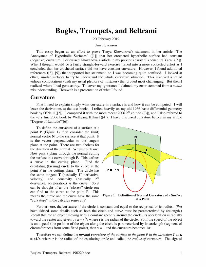
To define the curvature of a surface at a

point P (Figure 1), first consider the (unit)

normal vector N to the surface at that point. It

is the vector perpendicular to the tangent

plane at the point. There are two choices for

the direction of the normal. We just pick one.

Now pass a plane through the normal cutting

the surface in a curve through P. This defines

a curve in the cutting plane. Find the

osculating (kissing) circle to the curve at the

point P in the cutting plane. The circle has

the same tangent T (basically 1st derivative,

velocity) and concavity (basically 2nd

derivative, acceleration) as the curve. So it

can be thought of as the “closest” circle one

can find to the curve at the point P. This

means the circle and the curve have the same

“curvature” in the calculus sense at P.

Furthermore, the curvature of the circle is constant and equal to the reciprocal of its radius. (We

have skirted some details such as both the circle and curve must be parameterized by arclength.)

Recall that for an object moving with a constant speed v around the circle, its acceleration is radially

toward the center and given by a = v2/r where r is the radius of the circle. So if the speed of the object

is unit speed (the position of the object along the circle is parameterized by its arclength (segment of

circumference) from some fixed point), then v = 1 and the curvature becomes 1/r.

Therefore we can define the normal curvature of the surface at the point P in the direction T as κκκκ

= ±1/r, where r is the radius of the osculating circle and called the radius of curvature. The sign of

Figure 1 Definition of Normal Curvature of a Surface

at a Point


the curvature is given by the direction the tangent T is turning, that is, if T or the curve is turning

towards the normal N, then the sign is positive, and if it is turning away from N, then the sign is

negative.

Clearly, pivoting the surface-cutting plane about the normal will produce different curves in

different directions and therefore different normal curvatures. Unless the surface is like a sphere

where the normal curvature in any direction at the point P is the same (P is called an umbilic point),

the normal curvature will vary from a maximum to a minimum (and the corresponding radius of

curvature from a minimum to a maximum). These maximum and minimum curvatures are called the

principal curvatures of the surface at P and denoted k1 and k2. Furthermore, the directions giving

these maxima or minima are called principal directions and the corresponding unit tangent vectors

the principal vectors of the surface at P. It turns out that these principal vectors are always

orthogonal to each other.

We come now to the final main definition: The Gaussian curvature K of a surface at a point P is

the product of the principal curvatures at P, that is,

(Gaussian Curvature) K = k1·k2

Notice that we also have K = (1/r1)(1/r2) = (1/r1r2) where r1 and r2 are the radii of curvature of the

corresponding principal curvatures. The significant thing about the Gaussian curvature is that it is

intrinsic, that is, it is what someone living on the surface with no understanding of an embedding in a

higher dimension would calculate.

For example, for the surface shown in Figure 1, the tangents T will always be turning away from

the direction of the normal N, so both principal curvatures k1 and k2 are negative, their product is

positive, and so the resulting Gaussian curvature is positive.

Surface of Revolution

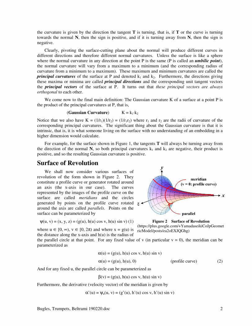
We shall now consider various surfaces of

revolution of the form shown in Figure 2. They

constitute a profile curve or generator rotated around

an axis (the x-axis in our case). The curves

represented by the images of the profile curve on the

surface are called meridians and the circles

generated by points on the profile curve rotated

around the axis are called parallels. Points on the

surface can be parameterized by

ψ(u, v) = (x, y, z) = (g(u), h(u) cos v, h(u) sin v) (1)

where u [0, ∞), v [0, 2π) and where x = g(u) is

the distance along the x-axis and h(u) is the radius of

the parallel circle at that point. For any fixed value of v (in particular v = 0), the meridian can be

parameterized as

α(u) = (g(u), h(u) cos v, h(u) sin v)

α(u) = (g(u), h(u), 0) (profile curve) (2)

And for any fixed u, the parallel circle can be parameterized as

β(v) = (g(u), h(u) cos v, h(u) sin v)

Furthermore, the derivative (velocity vector) of the meridian is given by

α’(u) = ψu(u, v) = (g’(u), h’(u) cos v, h’(u) sin v)

Figure 2 Surface of Revolution

(https://plus.google.com/+YamadaseikiCoJpGeomet

ricModel/posts/ea2oEXJQGhg)


and the derivative (velocity vector) of the

parallel is given by

β’(v) = ψv(u, v) = (0, –h(u) sin v, h(u) cos v)

Then the dot product of vectors α’(u) · β’(v) =

0 implies they are orthogonal and the meridians

and parallels are perpendicular to each other at

each point of the surface (Figure 3, based on

figures from [7]).

It should be evident (and can be calculated)

that the tangent vector α’(u) is pointing in a

principal direction, that is, that the normal

curvature at a point on the profile curve is

maximal (near the origin) and minimal (out

along the x-axis). That means that the vector

β’(v) tangent to the parallel at the same point and orthogonal to the profile tangent α’(u) must point in

the other principal direction. So the unit versions of these tangent vectors are the principal vectors at

each point of the surface of revolution. Curves in a surface whose tangent vectors all point in

principal directions are called principal curves. So the meridians and parallels of a surface of

revolution are principal curves.

This terminology confused me for some

time (and cost me several days of back and

forth computations). The curvature of the

parallel principal curve is not a principal

curvature! As you can see in Figure 3, the

parallel curve β(v) does not lie in a plane

through the unit normal N; it only shares the

unit tangent vector (principal vector) with the

osculating circle that does lie in the plane.

Figure 4 shows the relationship of the curvature

of a curve β whose tangent points in a principal

direction. If N(β) represents a unit normal to

this curve at some point P in the surface, then

the normal (principal) curvature kπ at P is

related to the (Frenét) curvature κ of β by ([2]

p.197)

kπ = κ N(β) · N = κ cosθ.

Since κ = 1/h is the curvature of the

parallel circle, the principal curvature

kπ = 1/rπ = cosθ / h ⇒ h = rπ cosθ .

This means the principal radius of curvature

in the parallel direction is the hypotenuse of

the right triangle with h as one leg and a

segment of the x-axis as the other. That means

the center of the osculating circle lies on the

x-axis, as shown in Figure 3 and Figure 4.

Also notice that radii of curvature rπ and

Figure 3 Surface of Revolution with Curvature

(Principal) Directions

Figure 4 ββββ Curve Curvature κκκκ vs Principal

Curvature kππππ

Figure 5 Radius of Curvature rππππ Sphere


rµ are on opposite sides of the tangent plane. This

means their corresponding curvatures will have

opposite signs. Therefore the product of these

curvatures, the Gaussian curvature, will be

negative.

By the rotational symmetry of the surface of

revolution, we see that the osculating circle sweeps

out a sphere centered on the x-axis (Figure 5).

This means for diagrammatic purposes we can

consider the osculating circle for rπ in the same

plane as the one for rµ (Figure 6).

We are now ready to consider different profile

curves and the different curvatures of the

corresponding surfaces of revolution.

Examples of Surfaces of Revolution

We now need to compute some explicit curvatures for several surfaces of revolution. I will use

the formulas and notation from O’Neill ([2] p.234, [3] p.253). Using the parameterized version of the

profile curve in equation (2), α(u) = (g(u), h(u), 0), we get the principal curvatures in the direction of

the meridian and parallel, along with the Gaussian curvature K, as:

( ) 2/322 ''

""

''

hg

hg

hg

k+

−

=µ , ( ) 2/122 ''

'

hgh

gk

+=π ,

( )222 ''

""

'''

hgh

hg

hgg

kkK+

−

== πµ (3)

In the case where g(u) = u, we get:

( ) 2/32'1

"

h

hk

+

−=µ ,

( ) 2/12'1

1

hhk

+=π ,

( )22'1

"

hh

hK

+

−= (4)

Hyperbola Profile – Torelli’s Trumpet

The first example is included because it is a standard example from calculus and has non-constant

negative curvature. The profile curve is α(u) = (u, h(u), 0) = (u, 1/u, 0) for 0 < u < ∞. The surface of

revolution is colorfully called Torelli’s Trumpet.

The surface area and volume of Torelli’s Trumpet are computed from improper integrals, usually

from some fixed point a > 0, say a = 1, over the whole positive real line. This entails taking the limits

of finite integrals over the closed intervals [a, b] where b → ∞. It turns out that the improper integral

for the surface area does not converge (have a limit as b → ∞), but the improper integral for the

volume does converge. Therefore one jokes that to paint the trumpet’s surface one must fill it with

paint instead. Thus the usual weird things happen when infinity is involved.

Using equations (4), we obtain the principal curvatures and Gaussian curvature

( ) 2/34

3

1

2

u

uk

+

−=µ ,

( ) 2/14

3

1 u

uk

+=π ,

( ) 2

3

24

6

1

2

1

1

1

2

+

−=+

−=

uu

u

uK

(See Figure 7). Notice that the radius of curvature of the parallel rπ = 1/kπ = (1/u2 + 1/u

6)

1/2 agrees

Figure 6 2-D Scheme for Computations


with the argument given above illustrated in Figure 4 where rπ is shown to be the hypotenuse of the

triangle with leg h(u) = 1/u. Notice that the angle θ in Figure 7 is the same as the angle θ in Figure 4.

tan θ represents the slope of the tangent to the profile curve or h’(u), and so equals 1/u2 (ignoring

signs). This implies the segment of the x-axis equals 1/u3 and so agrees with the value for rπ via the

Pythagorean Theorem.

Other things to notice are (1) the

length of the tangent line to the x-axis L

varies and (2) the x-distance of the

tangent point (x, y) to the center of the

osculating circle with radius rµ is rµ sin θ

= (u + 1/u3)/2.

Exponential Profile

We turn now to the example that instigated this investigation: my representation of Khovanova’s

crocheted “surface” as a surface of revolution with a profile curve of the form R2x. First, we will

convert this expression of doubling into the more customary form using the exponential function

y = ex via R2

x = Re

ln 2 x. This expression is an example of the general solution to the exponential

differential equation dy/dx = kx given by y = y0ekx

where y = y0 when x = 0. In other words y is the

general quantity that grows proportionally to its current value at any instant. For simplicity, we shall

set all constants equal to 1. Furthermore, we shall reverse the direction of Khovanova surface to

conform to the surface of revolution shapes we have been considering, namely, we shall consider

y = e-x

.

So the parameterization of the profile curve we are interested in is α(u) = (u, h(u), 0) = (u, e-u

, 0)

for 0 ≤ u < ∞. Since h’ = -h and h” = h, this yields the following principle curvatures and Gaussian

curvature:

Figure 7 Torelli’s Trumpet (hyperbolic profile curve) with Gaussian curvature K and radii of

curvature rππππ, rµµµµ

Figure 8 Trigonometric Relations


( ) 2/321 h

hk

+

−=µ ,

( ) 2/121

1

hhk

+=π ,

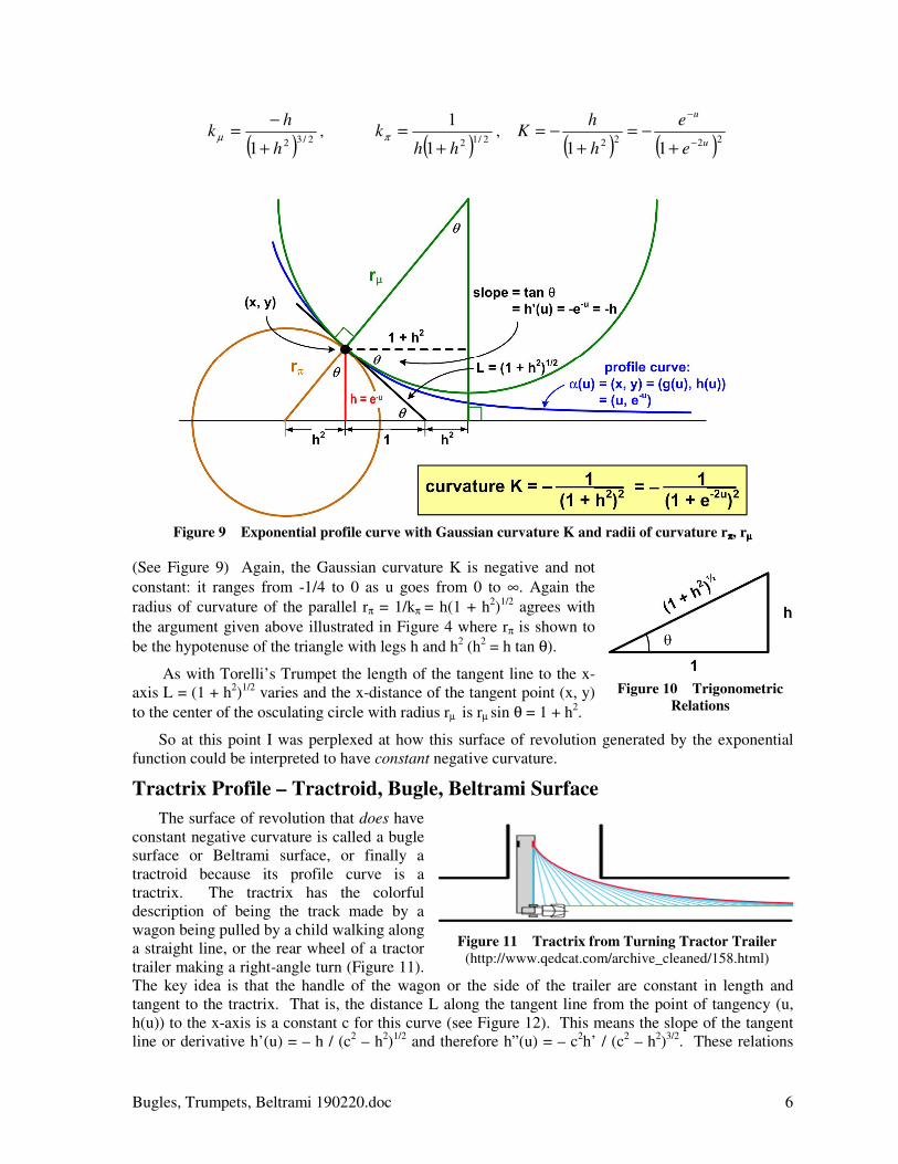
( ) ( )2222 11 u

u

e

e

h

hK

−

−

+−=

+−=

Figure 9 Exponential profile curve with Gaussian curvature K and radii of curvature rππππ, rµµµµ

(See Figure 9) Again, the Gaussian curvature K is negative and not

constant: it ranges from -1/4 to 0 as u goes from 0 to ∞. Again the

radius of curvature of the parallel rπ = 1/kπ = h(1 + h2)

1/2 agrees with

the argument given above illustrated in Figure 4 where rπ is shown to

be the hypotenuse of the triangle with legs h and h2 (h

2 = h tan θ).

As with Torelli’s Trumpet the length of the tangent line to the x-

axis L = (1 + h2)

1/2 varies and the x-distance of the tangent point (x, y)

to the center of the osculating circle with radius rµ is rµ sin θ = 1 + h2.

So at this point I was perplexed at how this surface of revolution generated by the exponential

function could be interpreted to have constant negative curvature.

Tractrix Profile – Tractroid, Bugle, Beltrami Surface

The surface of revolution that does have

constant negative curvature is called a bugle

surface or Beltrami surface, or finally a

tractroid because its profile curve is a

tractrix. The tractrix has the colorful

description of being the track made by a

wagon being pulled by a child walking along

a straight line, or the rear wheel of a tractor

trailer making a right-angle turn (Figure 11).

The key idea is that the handle of the wagon or the side of the trailer are constant in length and

tangent to the tractrix. That is, the distance L along the tangent line from the point of tangency (u,

h(u)) to the x-axis is a constant c for this curve (see Figure 12). This means the slope of the tangent

line or derivative h’(u) = – h / (c2 – h

2)

1/2 and therefore h”(u) = – c

2h’ / (c

2 – h

2)

3/2. These relations

Figure 10 Trigonometric

Relations

Figure 11 Tractrix from Turning Tractor Trailer

(http://www.qedcat.com/archive_cleaned/158.html)


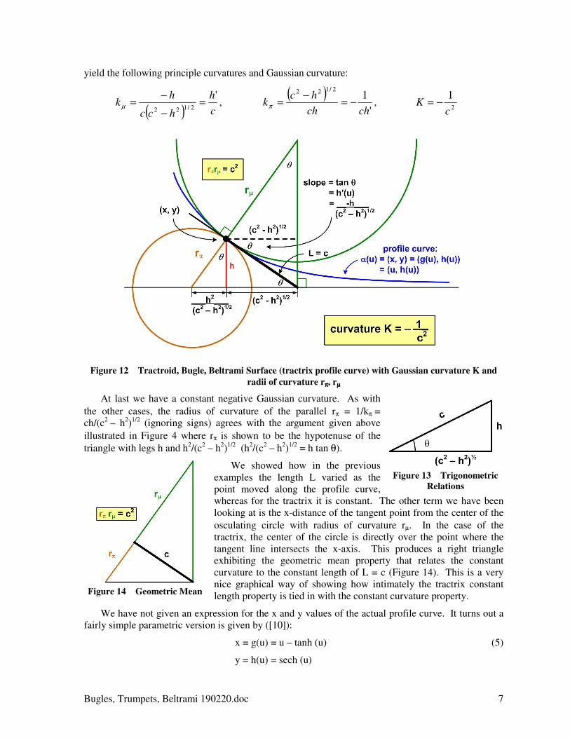
yield the following principle curvatures and Gaussian curvature:

( ) c

h

hcc

hk

'2/122

=−

−=µ ,

( )'

12/122

chch

hck −=

−=π ,

2

1

cK −=

Figure 12 Tractroid, Bugle, Beltrami Surface (tractrix profile curve) with Gaussian curvature K and

radii of curvature rππππ, rµµµµ

At last we have a constant negative Gaussian curvature. As with

the other cases, the radius of curvature of the parallel rπ = 1/kπ =

ch/(c2 – h

2)

1/2 (ignoring signs) agrees with the argument given above

illustrated in Figure 4 where rπ is shown to be the hypotenuse of the

triangle with legs h and h2/(c

2 – h

2)

1/2 (h

2/(c

2 – h

2)

1/2 = h tan θ).

We showed how in the previous

examples the length L varied as the

point moved along the profile curve,

whereas for the tractrix it is constant. The other term we have been

looking at is the x-distance of the tangent point from the center of the

osculating circle with radius of curvature rµ. In the case of the

tractrix, the center of the circle is directly over the point where the

tangent line intersects the x-axis. This produces a right triangle

exhibiting the geometric mean property that relates the constant

curvature to the constant length of L = c (Figure 14). This is a very

nice graphical way of showing how intimately the tractrix constant

length property is tied in with the constant curvature property.

We have not given an expression for the x and y values of the actual profile curve. It turns out a

fairly simple parametric version is given by ([10]):

x = g(u) = u – tanh (u) (5)

y = h(u) = sech (u)

Figure 13 Trigonometric

Relations

Figure 14 Geometric Mean


where u > 0.

Exponential Representation

This is all very fine, but where is the exponential that Khovanova and others said produced the

constant negative curvature? If we parameterize the tractrix by u = arclength, then the equations

become ([10]):

x = g(u) = ( ) 11ln 22 −−−+ − uuuu eeee (6)

y = h(u) = e-u

for u > 0. Finally, an explicit exponential for the y-values.

But parameterizations are tricky. The x-value parameterization must also be taken into account.

That is, we might think a curve given by y = h(u) = u2 represents a parabola, but if x = g(u) = u

2 as

well, then the curve is actually y = x or a straight line.

So what is going on? How is the tractrix profile curve parameterized by arclength related to the

exponential profile curve of the previous example? Hopefully Figure 15 provides the answer.

Figure 15 Tractrix vs. Exponential Profile Curves

I used the Igor analytic tool to plot three profile curves: the (green) exponential graph (u, e-u

), the

(black) tractrix using the parametric equations (5), and the (red) tractrix using the arclength

parameterized equations (6). I fattened the red curve to show how it coincided with the other

parameterization for the tractrix. S measures the arclength along the tractrix as well as the equal

horizontal distance to the exponential graph. The idea is that the y-value e-S

is the same in both cases.

My Error

So what was Tanya Khovanova really saying in her crochet posting and where did I go wrong?

Another picture should make it clear. I was effectively parameterizing the crochet loops along the x-

axis, that is, I was using equal horizontal spacing for the loops (Figure 16). Khovanova was

effectively using equal arclength spacing (Figure 17). If the figures are reversed to conform to the

surfaces of revolution we have been considering, then it is easy to see the same compression along the

x-axis for the arclength parameterization in Figure 17 is likewise shown in Figure 15.


Figure 16 Crochet Loops Equal Horizontal

Spacing

Figure 17 Crochet Loops Equal Arclength

Spacing

So Khovanova was really showing dC/ds = 2C where C is the circumference of the crochet loop

and s is the arclength measure along the surface. Since C = 2πr, we have dr/ds = 2r rather than

dr/dx = 2r as I was indicating. Thus the mystery is resolved. Details really matter in mathematics,

much to my consternation at times when I try to simplify things.

Addendum – Intrinsic Geometry I mentioned before that the

Gaussian curvature is a quantity

intrinsic to the surface. It is what

someone living in the surface would

measure. The statements about the

crocheted surface that rely on

arclength are of a similar nature

since arclength is what someone

would measure on the crochet

surface.

We can see a similar result for a

spherical surface with constant

positive curvature (Figure 18). The

“radius” of a circle in the surface centered at P is given by the arclength s = Rθ of the great circle

from the center to the circumference of the circle. The circumference C is parameterized by s via the

relations C = 2πr = 2πR sin θ = 2πR sin s/R. Therefore the rate of growth of the circumference C

with respect to “radius” s is

dC/ds = 2π cos s/R ≤ 2π

For a flat plane, the radius of a circle is the same as the arclength, so dC/ds = dC/dr = 2π, a

constant. Hence we see that a constant positive Gaussian curvature indicates a slower growth of the

circumference with respect to the “intrinsic” radius than in a flat plane. Similarly, as we saw with the

tractroid, for a constant negative Gaussian curvature we have dC/ds = 2π dr/ds = 2π k es ≥ 2π for

k > 1. So the growth of the circumference in this case is greater than 2π.

References [1] Khovanova, Tanya, “The Annoyance of Hyperbolic Surfaces” 27 November 2018

(https://blog.tanyakhovanova.com/2018/11/the-annoyance-of-hyperbolic-surfaces/)

[2] O’Neill, Barrett, Elementary Differential Geometry, Academic Press, 1966

Figure 18 Surface with Constant Positive Curvature


[3] O’Neill, Barrett, Elementary Differential Geometry, Revised Second Edition, Elsevier, 2006

[4] Kühnel, Wolfgang, Differential Geometry: Curves—Surfaces—Manifolds, 2nd

ed, (German)

2003, translated by Bruce Hunt, American Mathematical Society, 2006.

[5] Stevenson, James, “Exponential Yarn” in Meditations on Mathematics, 20 December 2018

(http://josmfs.net/2019/02/22/exponential-yarn/)

[6] Stevenson, James, “Degree of Latitude” in Meditations on Mathematics, 23 August 2011

(http://josmfs.net/2018/12/28/degree-of-latitude/)

[7] Saiki, “Curvature,” Hyperbolic Non-Euclidean World Part II, Ch.23, 22 February 2014

(http://www7a.biglobe.ne.jp/~saiki/us24b_rie.html, retrieved 12/9/2018)

[8] Apostol, Tom M. and Mamikon A. Mnatsakanian, “The method of sweeping tangents”

Mathematical Gazette, UK, 92, November 2008. pp.396-417 [pp.1-25]

(http://citeseerx.ist.psu.edu/viewdoc/download?doi=10.1.1.469.6231&rep=rep1&type=pdf,

retrieved 6/29/2014)

[9] “Hyperbolic Space” Wikipedia (https://en.wikipedia.org/wiki/Hyperbolic_space, retrieved

2/2/2019)

[10] Weisstein, Eric W., “Pseudosphere” MathWorld

(http://mathworld.wolfram.com/Pseudosphere.html, retrieved 12/15/2018)

© 2019 James Stevenson

bugles, trumpets, beltrami 190220 - josmfs.net

Documents