BROADBAND WAVEFORM MODELING OF

DEEP MANTLE STRUCTURE

by

Michael S. Thorne

A Dissertation Presented in Partial Fulfillment of the Requirements for the Degree

Doctor of Philosophy

ARIZONA STATE UNIVERSITY

December 2005

ABSTRACT

The lowermost 200 - 300 km of the mantle, known as the D" region, exhibits

some of the strongest seismic heterogeneity in the Earth and plays a crucial role in

thermal, chemical and dynamic processes in the mantle. Hot spot volcanism may

originate from the deep mantle in regions exhibiting the Earth’s most pronounced lateral

shear (S)-wave velocity gradients. These strong gradient regions display an improved

geographic correlation over S-wave velocities to surface hot spot locations. The origin of

hot spot volcanism may also be linked to ultra-low velocity zone (ULVZ) structure at the

core-mantle boundary (CMB). Anomalous boundary layer structure at the CMB is

investigated using a global set of broadband SKS and SPdKS waves from permanent and

portable seismometer arrays. The wave shape and timing of SPdKS data are analyzed

relative to SKS, with some SPdKS data showing significant delays and broadening. We

produce maps of inferred boundary layer structure from the global data and find evidence

for extremely fine-scale heterogeneity where our wave path sampling is the densest.

These data are consistent with the hypothesis that ULVZ presence (or absence) correlates

with reduced (or average) heterogeneity in the overlying mantle. In order to further

constrain deep mantle processes, synthetic seismograms for 3-D mantle models are

necessary for comparison with data. We develop a 3-D axi-symmetric finite difference

(FD) algorithm to model SH-wave propagation (SHaxi). In order to demonstrate the

utility of the SHaxi algorithm we apply the technique to whole mantle models with

random heterogeneity applied to the background model producing whole mantle

scattering. We also apply SHaxi to model SH-wave propagation through cross-sections

iii

of 3-D lower mantle D" discontinuity models beneath the Cocos Plate derived from

recent data analyses. We utilize double-array stacking to assess model predictions of data.

3-D model predictions show waveform variability not observed in 1-D model predictions,

demonstrating the importance for the 3-D calculations. An undulating D" reflector

produces a double Scd arrival that may be useful in future studies for distinguishing

between D" volumetric heterogeneity and D" discontinuity topography.

iv

Dedicated to

Peggy Louise Thorne

v

ACKNOWLEDGMENTS

My greatest appreciation goes to my advisor Ed Garnero. Many thanks for

drawing me away from the engineering field and opening my way into seismology. Ed

Garnero has proven the best of advisors for many reasons. The exhilaration and interest

he displays when shown something new in the seismic wavefield is infectious and

inspiring. His creativity in giving suggestions on how to solve problems has always been

greatly appreciated. As highly regarded is his hands-off approach in allowing one to

arrive at one’s own conclusions and in problem solving. Thank you for the constant

support, advice, and sometimes silence.

Thanks to my supervisory committee Matt Fouch, Jim Tyburczy, John Holloway

and Simon Peacock for many valuable discussions. Special thanks to Matt Fouch for

always having an open door and for giving such good advice throughout the years.

Additional thanks to Allen McNamara who should have also been on my committee.

Special thanks to Ed’s other students and post docs with whom I have shared lab

space and a variety of experiences over the years. Thanks to Melissa Moore for

continually keeping me entertained with her moaning, whimpering, grunting and general

utterances as to how her work progressed. Thanks to Nicholas Schmerr for an

enlightening number of years of discussion on the transition zone, tornados, and just

about everything else one could imagine. Most notably, thank you for providing ample

buffer from the boundless string of flippant GCC neophyte questions. An innumerable

amount of thanks must also go to Sean Ford, who has single handedly brought SACLAB

into the seismological mainstream, entertained us all with tales of complex signal

vi

analysis dalliances, and kept a positive light over even the darkest of GCC days. A day

without Sean is like a day without sunshine. Many more thanks need to go to Sebastian

Rost than can be listed here, but thank you in general for all of the discussion and advice

given over the years.

I would like to give thanks to those with whom I have become close friends with

in my three visits to Bavaria. Special thanks to Markus, Rosemary, Hanna and Martin

Treml for all the times you have housed and fed me when I came to Munich. Special

thanks to Markus for all of the amazing trips you have taken me on, from hiking in the

Alps, to visiting ancient monasteries to spending a day at the Wiesn. Thanks to Gunnar

Jahnke for sharing your first version of the SHaxi code with me on the first day we met,

and for being such a great collaborator ever since. Thanks to Heiner Igel for support and

the willingness to bring me to Munich three times. Thanks to Franz Antwetter for letting

me stay one summer in your flat. Thanks to Gilbert Brietzke, Toni Kraft, and Tobi Metz

for also making my stays in Munich much more enjoyable and for oftentimes staying out

with me until the first U-Bahn train started running in the morning. Thanks to Hubert for

making elefontastic programming accessible even to me. Thanks to Guoquan Wang for

sharing an office with me during the sweltering summer of 2003, for allowing me to open

the window from time to time and most notably for sharing the esoteric teachings of The

Book of Chinese Seismology with me. Many thanks to the rest of Heiner’s students that I

have not mentioned above for making my stays in Munich more enjoyable.

Thanks to Artie Rodgers for an enjoyable summer at LLNL. Also thanks to Steve

Meyers, Dave Harris and Hrvoje Tkalčić for their technical expertise. Thanks to Clipper

vii

Ford for giving me a place to stay in Livermore and to Bazo for giving me a computer to

use while I was there.

I have also received gracious support from many other graduate students over the

last few years. Most notably, thanks to John Hernlund, Tarje Nissen-Meyer, and Megan

Avants. Thanks to Adam Baig for an especially wild time in the Canadian Northwest.

Thanks to the graduate students of Matt Fouch and Allen McNamara with whom I have

shared our computer lab and many enjoyable experiences over the last several years,

Jesse L. Yoburn, Teresa Lassak, Karen Anglin, and Abby Bull.

I would like to give special thanks to the systems administrators who have served

our lab. Somehow they managed, apparently while under great personal duress, to

maintain our network and still occasionally manage to install a piece of software for me

here or there. Thanks to Bruce Tachoir, Marvin Simkin and Mark Stevens. Also thanks

to Christoper Puleo, web designer extraordinaire, for help with web design and various

beautiful photoshop art projects. Many thanks to Jeff Lockridge for maintaining our PC’s

and our PDF library.

Finally I would like to acknowledge Dawn Ashbridge without whom I can’t

conceive of having finished this dissertation. I would also like to acknowledge my father,

Robert Thorne, for his support through this endeavor. And very special thanks to some

of my closest friends in Arizona whose companionship in backpacking adventures across

the southwest have helped to keep me sane. Special thanks to Todd A. Jones, Stephen T.

Wiese, Shinichi Miyazawa, Trevor Graff, and David Downham.

viii

TABLE OF CONTENTS

Page LIST OF TABLES........................................................................................................... xiii LIST OF FIGURES ......................................................................................................... xiv PREFACE...................................................................................................................... xviii CHAPTER 1. GENERAL INTRODUCTION....................................................................1

2. GEOGRAPHIC CORRELATION BETWEEN HOT SPOTS

AND DEEP MANTLE LATERAL SHEAR-WAVE VELOCITY GRADIENTS..........................................................................6

Summary ..............................................................................................6 2.1 Introduction...................................................................................7 2.2 Calculation of lateral shear-wave velocity gradients ..................11 2.3 Results.........................................................................................13 2.4 Discussion ...................................................................................15 2.5 Conclusions.................................................................................26 Acknowledgements............................................................................28 References..........................................................................................28 Tables.................................................................................................36 Figures................................................................................................40 Supplemental Figures.........................................................................51

ix

CHAPTER Page

3. INFERENCES ON ULTRALOW-VELOCIY ZONE STRUCTUE FROM A GLOBAL ANALYSIS OF SPDKS WAVES............................61 Summary ............................................................................................61 3.1 Introduction.................................................................................62 3.2 SPdKS data..................................................................................69 3.3 Synthetic seismograms................................................................73 3.4 Modeling approach .....................................................................77 3.5 Inferred ULVZ distribution.........................................................83 3.6 Discussion ...................................................................................90 3.7 Conclusions.................................................................................99 Acknowledgements..........................................................................100 References........................................................................................101 Tables...............................................................................................109 Figures..............................................................................................114 Supplemental Figures.......................................................................132 4. COMPUTING HIGH FREQUENCY GLOBAL SYNTHETIC SEISMOGRAMS USING AN AXI-SYMMETRIC FINITE DIFFERENCE APPROACH .....................................................134 4.1 Introduction...............................................................................134 4.2 3-D Axi-Symmetric Finite Difference Wave Propagation .......136 4.3 Finite Difference Implementation.............................................140 4.4 Application: Whole Mantle Scattering ....................................147

x

CHAPTER Page 4.5 Conclusions...............................................................................160 Acknowledgements..........................................................................162 References........................................................................................162

Tables...............................................................................................167 Figures..............................................................................................168 5. 3-D SEISMIC IMAGING OF THE D" REGION BENEATH THE COCOS PLATE .............................................................................195 Summary ..........................................................................................195 5.1 Introduction...............................................................................196 5.2 3-D axi-symmetric finite difference method and verification ..202 5.3 Study region and model construction .......................................205 5.4 Synthetic seismogram results....................................................211 5.5 Synthetic seismograms compared with data .............................216 5.6 Double-array stacking comparisons..........................................217 5.7 Discussion .................................................................................219 5.8 Conclusions...............................................................................223 Acknowledgements..........................................................................225 References........................................................................................226 Tables...............................................................................................232 Figures..............................................................................................234 Supplemental Figures.......................................................................246

xi

APPENDIX Page A. COMPANION CD..................................................................................256

A.1 SACLAB...................................................................................257 A.2 Animations of Seismic Wave Propagation ...............................259

xii

LIST OF TABLES

Table Page

2.1 S-wave velocity models analyzed in this study....................................................36

2.2 Hot spots used with locations ..............................................................................37

2.3 S-wave velocity percent coverage of CMB surface area overlain by each hotspot ....................................................................................................38

2.4 Lateral gradient percent coverage of CMB surface area overlain

by each hotspot ....................................................................................................39 3.1 Core-Mantle Boundary Layer Studies ...............................................................109 3.2 Earthquakes Used in This Study ........................................................................110 3.3 Synthetic Model Space Parameter Ranges ........................................................111 3.4 Model Parameters Corresponding to Figure 3.7 ................................................112 3.5 Average CMB Layer Thickness.........................................................................113 4.1 Example SHaxi Parameters and Performance ...................................................167 5.1 D" models investigated ......................................................................................232 5.2 D" thickness (km) from double-beam stacking for data and models.................233 A.1 Core SACLAB routines and function ................................................................258

xiii

LIST OF FIGURES

Figure Page 2.1 Location of hot spots used in this study...............................................................40 2.2 Hot spot hit counts for model S20RTS................................................................41 2.3 S-wave velocity models and lateral S-wave velocity gradients ...........................43 2.4 Hot spot hit counts for model S20RTS................................................................45 2.5 Overall hot spot hit counts ...................................................................................46 2.6 S-wave velocity model standard deviation ..........................................................47 2.7 Hot spot deflections .............................................................................................48 2.8 Average hot spot hit counts at four depths in Earth’s mantle ..............................50 2A SAW12D velocities and gradients .......................................................................51 2B S14L18 velocities and gradients ..........................................................................53 2C S20RTS velocities and gradients..........................................................................55 2D S362C1 velocities and gradients ..........................................................................57 2E TXBW velocities and gradients...........................................................................59 3.1 Past ULVZ study results ....................................................................................114 3.2 Seismic phases used in this study ......................................................................115 3.3 Distance profiles for four events........................................................................116 3.4 Station profiles for four stations ........................................................................117 3.5 ULVZ, CRZ, and CMTZ model profiles ...........................................................118 3.6 Empirical source modeling ................................................................................119 3.7 Cross-correlation of records with model synthetics...........................................121 3.8 PREM synthetics and SKiKS observations ........................................................123

xiv

Figure Page

3.9 Data coverage by epicentral distance and average cross-correlation

coefficients........................................................................................................124

3.10 SPdKS observations for the southwest Pacific and Central American

regions...............................................................................................................125 3.11 Data coverage, ULVZ likelihood, and average ULVZ thickness.....................126 3.12 SPdKS Fresnel zones.........................................................................................128 3.13 Comparison between SPdKS source and receiver side arcs with S- and P- wave velocity structure .....................................................................129 3.14 SPdKS ray path geometry for different ULVZ locations..................................130 3A ULVZ likelihood map comparison ...................................................................132 4.1 Spherical coordinate system used in SHaxi .......................................................168 4.2 SHaxi grid and parallelization ...........................................................................169 4.3 SHaxi staggered grid..........................................................................................171 4.4 SHaxi source radiation pattern...........................................................................172 4.5 High and low velocity anomalies on SHaxi grid ...............................................173 4.6 3-D axi-symmetric ring structure.......................................................................174 4.7 Snapshots of wave propagation in PREM model ..............................................175 4.8 PREM synthetic seismograms ...........................................................................177 4.9 Random seed matrices .......................................................................................179 4.10 Bessel functions of the second kind...................................................................180 4.11 1-D autocorrelation functions ............................................................................181 4.12 Isotropic random media .....................................................................................182

xv

Figure Page 4.13 Power spectra of random media in Figure 4.12 .................................................184 4.14 Anisotropic random media.................................................................................185 4.15 Snapshots of wave propagation in homogeneous media ...................................187 4.16 Snapshots of wave propagation in random media .............................................189 4.17 Realization of random media in SHaxi..............................................................191 4.18 Axi-symmetric representation of random media in SHaxi ................................192 4.19 Frequency dependence of scattering effects ......................................................193 4.20 Effect of autocorrelation length on waveform properties ..................................194 5.1 D" discontinuity model synthetic seismograms.................................................234 5.2 SH- velocity wavefield for a D" model..............................................................236 5.3 Location of study region ....................................................................................238 5.4 SH- velocity wavefield for a topographically varying D" discontinuity model............................................................................................239 5.5 Comparison of synthetics for model TXBW .....................................................241 5.6 Comparison of synthetics with data...................................................................242 5.7 Double-beam stacking results ............................................................................244 5.8 3-D effects of D" lateral S-wave velocity heterogeneity ...................................245 5A PREM synthetics with crustal and mid-crustal arrivals .....................................246 5B Lower mantle cross-sections for models LAYB and THOM .............................248 5C Lower mantle cross-sections and velocity profile for model TXBW .................249 5D Whole mantle cross-sections for model TXBW .................................................250 5E Comparison of 1-D synthetics with model LAYB..............................................252

xvi

Figure Page 5F Comparison of synthetics form THOM1.5 and THOM2.0 .................................254

xvii

PREFACE The format and content of each chapter conform to the author guidelines of

Geophysical Journal International. Chapter 2, Geographic Correlation Between Hot

Spots and Deep Mantle Lateral Shear-Wave Velocity Gradients was published in Physics

of the Earth and Planetary Interiors, Volume 146, Issues 1-2, pages 47-63, 2004. Chapter

3, Inferences on Ultralow-Velocity Zone Structure from a Global Analysis of SPdKS

waves was published in Journal of Geophysical Research – Solid Earth, Volume 109,

B08301, doi:10.1029/2004JB003010, pages 1-22, 2004. The first part of Chapter 4,

Computing High Frequency Global Seismograms Using and Axi-Symmetric Finite

Difference Approach describes the mathematics and computation of a new technique for

producing synthetic seismograms (SHaxi) and is original to this dissertation. The second

part of Chapter 4 describes an application of this SHaxi method for computing synthetic

seismograms for models with random velocity perturbations. Some of the results

presented in Chapter 4, are submitted to Geophysical Journal International in the paper,

Global SH-Wave Propagation Using a Parallel Axi-Symmetric Finite Difference Scheme

by Gunnar Jahnke, Michael Thorne, Alain Cochard and Heiner Igel. Chapter 5, 3-D

Seismic Imaging of the D" Region Beneath the Cocos Plate was submitted to Geophysical

Journal International in Sept. 2005.

xviii

CHAPTER 1

GENERAL INTRODUCTION

Ever since the designation of the D" region (Bullen 1949), consisting of

heterogeneous velocity structure in the lowermost 200-300 km of the mantle, researchers

have sought to characterize the detailed nature of this boundary layer. The mechanisms

responsible for D" heterogeneity, manifested in strong arrival time fluctuations of seismic

phases sampling the region, are still poorly constrained. In the past decade increasing

evidence suggests that processes responsible for this deep mantle heterogeneity are linked

to whole mantle processes and surface features. For example, deep mantle high seismic

wave speeds have been linked to regions of past subduction (e.g., Dziewonski, 1984).

Recently, seismic tomography has also imaged high seismic velocity structures

resembling subducting slabs plunging deep into the mantle (e.g., Grand et al. 1997; van

der Hilst et al. 1997). These subducting slabs may plunge all the way to the core-mantle

boundary (CMB) in turn giving rise to the discontinuous increase in seismic velocities

200-300 km above the CMB known of as the D" discontinuity. However, other

explanations for the origin of the D" discontinuity abound, and the recent discovery of a

deep mantle phase transition from magnesium silicate perovskite to a post-perovskite

structure (e.g., Tsuchiya et al. 2004) has invigorated the debate. In this dissertation we

examine surface features such as hot spot volcanism and compare them to deep mantle

seismic observables. Furthermore we analyze broadband seismic energy sampling the

deepest mantle in effort to put constraint on the possible origins of deep mantle

heterogeneity and its relation to whole mantle processes and surface features.

2

Hot spot volcanism may originate in the deep mantle. Previous studies have

indicated that this volcanism is correlated with regions of the deepest mantle where low

S-wave velocities are resolved in global tomographic models (e.g., Wen & Anderson,

1997). In Chapter 2 we compare the surface location of hot spots to deep mantle S-wave

velocities and lateral S-wave velocity gradients. We show that hot spot volcanism may

originate from the deep mantle in regions exhibiting Earth’s most pronounced lateral S-

wave velocity gradients. These strong gradient regions display an improved geographic

correlation over S-wave velocities to surface hot spot locations. Furthermore, we find

that strong gradient regions typically surround the large lower velocity regions in the base

of the mantle, which may indicate a possible chemical, in addition to thermal, component

to these regions.

A connection between the origin of mantle plumes in the deep mantle and ultra-

low velocity zones (ULVZs) has recently been advanced (e.g., Williams et al. 1998).

Ultra-low velocity zones are roughly 10-40 km thick regions at the base of the mantle

with S- and P-wave velocity reductions of as much as 40% and 10% respectively. These

ULVZs may be regions of partial melt located at the hottest regions of the CMB. In order

to understand their relationship with regions of mantle upwelling we analyzed a global

dataset of SKS and SPdKS waveforms. The wave shape and timing of SPdKS data are

analyzed relative to SKS, with some SPdKS data showing significant delays and

broadening. We find evidence for extremely fine-scale heterogeneity and produce new

maps of inferred ULVZ distribution. Furthermore, we show that our data are consistent

3

with the hypothesis that ULVZ presence (or absence) correlates with reduced (or

average) heterogeneity in the overlying mantle.

In Chapter 3 we modeled SPdKS waveforms using the 1-D reflectivity technique

(Müller, 1985). However, in this modeling endeavor we found it challenging to explain

some of the SPdKS waveform complexity using a purely 1-D technique. Because short

scale-length lateral heterogeneity at the CMB could account for the waveform distortions

we sought to utilize techniques at predicting the seismic wavefield in 2- or 3-D. This

prompted us to work on techniques for synthesizing waveforms for models of higher-

dimensional complexity. In Chapter 4 we discuss one such technique for propagating

seismic energy for SH-waves in 3-D axi-symmetric models (SHaxi). We discuss

solutions to the axi-symmetric wave equation and the numerical application of this

technique. Furthermore, we assess the technique’s performance on modern distributed

memory architectures and discuss the limitations and advantages of using the axi-

symmetric assumption.

In order to demonstrate the versatility of the SHaxi technique we apply the

method to compute synthetic seismograms for models containing whole mantle random

velocity perturbations. Random velocity perturbations or random media, produce

scattering of the seismic wavefield. Scattering from random media in turn produces

seismic coda or a train of arrivals occurring after the main seismic arrivals. For S-wave

propagation seismic coda have been extensively studied at high frequency for regional

distances (e.g., Sato & Fehler 1998), in which the effects of scattering on the wavefield

have been demonstrated to be limited to short period and broadband seismic observations

4

contributing to the total attenuation of the waveforms. However, the computational cost

of performing numerical simulations at high frequencies has prevented computation of

synthetic seismograms for global models containing random media. We compute

synthetic seismograms for whole mantle random media and examine the effects of

random heterogeneity on the seismic waveforms.

As a further application of the SHaxi technique developed in Chapter 4, in

Chapter 5 we apply the method to compute synthetic seismograms for recent models of

D" discontinuity structure beneath the Cocos Plate region. The D" discontinuity beneath

the Cocos Plate region has received a considerable amount of recent attention in the past

two years and several possible 3-D models for its structure have been proposed. Yet,

these 3-D models have all been constructed using 1-D techniques and have never been

benchmarked with synthetics produced with 3-D techniques. We compute synthetic

seismograms for these recent models of discontinuity structure and compare them with

broadband data. We assess the ability of each model to predict the timing of seismic

arrivals traversing the deep mantle and make an analysis of future processing steps

necessary in order to gain a finer scale 3-D picture of the deep mantle.

5

REFERENCES

Bullen, K. E., 1949. Compressibility-pressure hypothesis and the Earth's interior, Monthly Notes of the Royal Astronomical Society, Geophysics Supplement, 355-368.

Dziewonski, A.M., 1984. Mapping the lower mantle - Determination of lateral

heterogeneity in P-velocity up to degree and order-6. Journal of Geophysical Research, 89 (NB7), 5929-5952.

Grand, S.P., van der Hilst, R.D. & Widiyantoro, S., 1997. Global seismic tomography: a

snapshot of convection in the Earth. GSA Today, 7 (4), 1-7. Müller, G., 1985. The Reflectivity Method - a Tutorial, Journal of Geophysics-Zeitschrift

Fur Geophysik, 58 (1-3), 153-174. Sato, H., & Fehler, M.C., 1998. Seismic Wave Propagation and Scattering in the

Heterogeneous Earth, Springer-Verlag, New York, 308 pages. Tsuchiya, T., Tsuchiya, J., Umemoto, K. & Wentzcovitch, R. A., 2004. Phase transition

in MgSiO3 perovskite in the Earth’s lower mantle, Earth and Planetary Science Letters, 224, 241-248.

Van der Hilst, R.D., Widiyantoro, S., & Engdahl, E.R., 1997. Evidence for deep mantle

circulation from global tomography, Nature, 386 (6625), 578-584. Wen, L.X. & Anderson, D.L., 1997. Slabs, hotspots, cratons and mantle convection

revealed from residual seismic tomography in the upper mantle. Phys. Earth Planet. Inter., 99 (1-2), 131-143.

Williams, Q., J. Revenaugh, & E. Garnero, 1998. A correlation between ultra-low basal

velocities in the mantle and hot spots, Science, 281 (5376), 546-549.

CHAPTER 2

GEOGRAPHIC CORRELATION BETWEEN HOT SPOTS AND DEEP MANTLE

LATERAL SHEAR-WAVE VELOCITY GRADIENTS

Michael S. Thorne1, Edward J. Garnero1, and Stephen P. Grand2

1Dept. of Geological Sciences, Arizona State University, Tempe, AZ 85287, USA 2Dept. of Geological Sciences, University of Texas at Austin, Austin, TX 78712, USA SUMMARY

Hot spot volcanism may originate from the deep mantle in regions exhibiting the Earth’s

most pronounced lateral S-wave velocity gradients. These strong gradient regions display

an improved geographic correlation over S-wave velocities to surface hot spot locations.

For the lowest velocities or strongest gradients occupying 10% of the surface area of the

core-mantle boundary (CMB), hot spots are nearly twice as likely to overlie the

anomalous gradients. If plumes arise in an isochemical lower mantle, plume initiation

should occur in the hottest (thus lowest velocity) regions, or in the regions of strongest

temperature gradients. However, if plume initiation occurs in the lowest velocity regions

of the CMB lateral deflection of plumes or plume roots are required. The average lateral

deflections of hot spot root locations from the vertical of the presumed current hot spot

location ranges from ~300-900 km at the CMB for the 10-30% of the CMB covered by

the most anomalous low S-wave velocities. The deep mantle may, however, contain

strong temperature gradients or be compositionally heterogeneous, with plume initiation

in regions of strong lateral S-wave velocity gradients as well as low S-wave velocity

regions. If mantle plumes arise from strong gradient regions, only half of the lateral

deflection from plume root to hot spot surface location is required for the 10-30% of the

CMB covered by the most anomalous strong lateral S-wave velocities. We find that

7

strong gradient regions typically surround the large lower velocity regions in the base of

the mantle, which may indicate a possible chemical, in addition to thermal, component to

these regions.

2.1 Introduction

2.1.1 Seismic evidence for mantle plumes

Morgan (1971) first proposed that hot spots may be the result of thermal plumes

rising from the core-mantle boundary (CMB). This plume hypothesis has gained

widespread appeal, yet direct seismic imaging of whole mantle plumes through travel-

time tomography or forward body wave studies have not yet resolved this issue (e.g., Ji &

Nataf 1998b; Nataf 2000). Plume conduits are predicted to be on the order of 100 – 400

km in diameter, with maximum temperature anomalies of roughly 200 – 400 K (Loper &

Stacey 1983; Nataf & Vandecar 1993; Ji & Nataf 1998a). Global tomographic models

typically possess lower resolution than is necessary to detect a plume in its entirety.

Table 2.1 lists the resolution for several recent whole mantle tomographic models.

However, a few higher resolution tomographic studies have inferred uninterrupted low

velocities from the CMB to the base of the crust. For example, the models of Bijwaard &

Spakman (1999) (65 – 200 km and 150 – 400 km lateral resolution in upper and lower

mantle, respectively) and Zhao (2001) (5 deg lateral resolution) both show uninterrupted

slow P-wave velocities beneath Iceland, which have been interpreted as evidence for a

whole mantle plume in the region. In addition, the tomographic model S20RTS (Ritsema

et al. 1999; Ritsema & van Heijst 2000) shows a low S-wave velocity anomaly in the

8

upper mantle beneath Iceland that ends near 660 km depth. High resolution (e.g., block

sizes of 75 × 75 × 50 km, Foulger et al. 2001) regional tomographic studies have also

been used to image plumes in the upper mantle and have shown that some plumes extend

at least as deep as the transition zone, but the full depth extent of the inferred plumes

remains unresolved (Wolfe et al. 1997; Foulger et al. 2001; Gorbatov et al. 2001).

Resolution at even shorter scale lengths is necessary to determine with greater confidence

any relationship between continuity of low velocities in the present models and mantle

plumes.

Several body wave studies have focused on plume-like structures related to hot

spots at the base of the mantle. For example, Ji & Nataf (1998b) used a method similar to

diffraction tomography to image a low velocity anomaly northwest of Hawaii that rises at

the base of the mantle and extends at least 1000 km above the CMB. Helmberger et al.

(1998) used waveform modeling to show evidence for a 250 km wide dome-shaped,

ultra-low velocity zone (ULVZ) structure beneath the Iceland hot spot at the CMB. Ni et

al. (1999) used waveform modeling to confirm the existence of an anomalous

(approximately up to -4% δVs) low velocity structure beneath Africa extending upward

1500 km from the CMB, which may be related to one or more of the hot spots found in

the African region. Several seismic studies have shown evidence for plumes in the

mantle transition zone (410 – 660 km), suggesting that hot spots may feed plumes at a

minimum depth of the uppermost lower mantle (Nataf & Vandecar 1993; Wolfe et al.

1997; Foulger et al. 2001; Niu et al. 2002; Shen et al. 2002). These plumes are not

necessary to explain the majority of hot spots on Earth’s surface (Clouard & Bonneville

9

2001), but suggest that some hot spots may be generated from shallow upwelling as

implied by layered convection models (e.g., Anderson 1998).

2.1.2 Indirect evidence: correlation studies

The inference that the deepest mantle seismic structure is related to large-scale

surface tectonics has been given much attention in the past decade (e.g., Bunge &

Richards 1996; Tackley 2000). Several studies suggest that past and present surface

subduction zone locations overlay deep mantle high seismic wave speeds (Dziewonski

1984; Su et al. 1994; Wen & Anderson 1995), which are commonly attributed to cold

subducting lithosphere migrating to the CMB. Recent efforts in seismic tomography

have revealed images of planar seismically fast structures resembling subducting

lithosphere that may plunge deep into the mantle (Grand 1994; Grand et al. 1997; van der

Hilst et al. 1997; Bijwaard et al. 1998; Megnin & Romanowicz, 2000; Gu et al. 2001).

The final depth of subduction has far reaching implications for the nature of mantle

dynamics and composition (Albarede & van der Hilst 2002). This finding, coupled with

the spatial correlation of hot spots and deep mantle low seismic velocities, are main

constituents of the argument for whole mantle convection (Morgan 1971; Hager et al.

1985; Ribe & Devalpine 1994; Su et al. 1994; Grand et al. 1997; Lithgow-Bertelloni &

Richards 1998).

With present challenges in direct imaging of mantle plumes or the source of hot

spots, comparison studies of hot spots and deep mantle phenomena have yielded

provocative results. Surface locations of hot spots have been correlated to low velocities

10

(e.g., Wen & Anderson 1997; Seidler et al. 1999) and ULVZs (Williams et al. 1998) at

the CMB. It has also been noted, however, that the locations of hot spots at Earth’s

surface tend to lie near edges of low-velocity regions, as shown by tomographic models

at the CMB (Castle et al. 2000; Kuo et al. 2000). This correlation has been used to imply

that mantle plumes can be deflected by more than 1000 km from their proposed root

source of the deepest mantle lowest velocities to the surface, perhaps by the action of

“mantle winds” (e.g., Steinberger 2000).

2.1.3 Other mantle plume studies

The wide variability of observed and calculated hot spot characteristics implies

that several mechanisms for hot spot genesis may be at work. Modeling of plume

buoyancy flux has been carried out for several hot spots (Davies 1988; Sleep 1990; Ribe

& Christensen 1994), revealing a wide range in the volcanic output of plumes possibly

responsible for many hot spots. Geodynamic arguments suggest some hot spots may be

fed by shallow-rooted (e.g., Albers & Christensen 1996) or mid-mantle-rooted (e.g.,

Cserepes and Yuen 2000) plume structures. Geochemical evidence suggests that

different hot spot source regions may exist (Hofmann 1997), as shown by isotopic studies

that argue for either transition zone (e.g., Hanan and Graham 1996) or CMB (e.g.,

Brandon et al. 1998; Hart et al. 1992) source regions. Further tomographic evidence has

been used to argue that several hot spots may be fed by a single large upwelling from the

deep mantle (e.g., Goes et al. 1999). Hence, the original mantle plume hypothesis

11

(Morgan 1971), that long-lived thermal plumes rise from the CMB, has expanded to

include a wide variety of possible origins of hot spot volcanism.

In this study, we explore statistical relationships between the surface locations of

hot spots and seismic heterogeneity observed in the deep mantle. Specifically, we

compare hot spot surface locations to low S-wave velocity heterogeneities and strong S-

wave lateral velocity gradients. We evaluate the origin of hot spot related plumes, and

examine the implications for deep mantle composition and dynamics.

2.2 Calculation of lateral shear-wave velocity gradients

We analyzed gradients in lateral S-wave velocity at the CMB for six global

models of S-wave velocities. Table 2.1 summarizes the parameterizations of each of the

models analyzed. Using bi-cubic interpolation, we resampled models originally

parameterized in either spherical harmonics or blocks onto a 1x1 degree grid.

Additionally, we smoothed block models laterally by Gaussian cap averaging with a

radius of 4 or 8 degrees for comparison with the smoother structures represented by

spherical harmonics. We calculated lateral S-wave velocity gradients for the deepest

layer in each model at every grid point as follows: (a) great circle arc segments were

defined with 500 to 2000 km lengths centered on each grid point for every 5 degrees of

rotation in azimuth; (b) seismic velocity was estimated at 2, 3, 5, 7, or 9 equally spaced

points (by nearest grid point interpolation) along each arc; (c) a least squares best fit line

through arc sampling points was applied for each azimuth; and (d) the maximum slope,

or gradient, and associated azimuth was calculated for each grid point. This approach

12

proved versatile for computing lateral velocity gradients for the variety of model

parameterizations analyzed (Table 2.1).

In order to compare S-wave velocities and lateral S-wave velocity gradients

between different models, lower mantle S-wave velocities and lateral S-wave velocity

gradients were re-scaled according to CMB surface area. For example, for model

S20RTS, S-wave velocities at or lower than δVs = -1.16, 10% of the surface area of the

CMB is covered (herein after referred to as “% CMB surface area coverage”). Similarly,

the most anomalous velocities occupying 20% CMB surface area coverage, are lower

than δVs = -0.59. Lateral S-wave velocity gradients are scaled in the same manner,

where 10% CMB surface area coverage corresponds to the most anomalous strong

gradients. The number of hot spots located within a given percentage of CMB surface

area coverage for low S-wave velocity or strong lateral gradient are tabulated into hot

spot hit counts. In this manner, the spatial distribution of the most anomalous low

seismic velocities and strong gradients can be equally compared and correlated to hot

spots. For example, the first two columns of Figure 2.2 show velocities and gradients of

the model S20RTS (Ritsema & van Heijst 2000), with contours drawn in green around

the 10, 20, and 30% most anomalously low shear velocities and strongest lateral S-wave

velocity gradients scaled by CMB surface area coverage. In the third column (Fig. 2.2),

the % CMB surface area coverage contours are filled in solid, with hot spot positions

drawn as red circles and hot spot hit counts listed beneath the respective globes.

In order to compare shear velocities and our computed lateral S-wave velocity

gradients to hot spot surface locations, we used a catalog of 44 hot spots (Steinberger

13

2000). We used this catalog because it imposed three stringent conditions to qualify as a

hot spot. First, each hot spot location must be associated with a volcanic chain, or at least

two age determinations must exist indicating a volcanic history of several million years.

Second, two out of four of the following conditions must be met: (i) present-day or

recent volcanism, (ii) distinct topographic elevation, (iii) associated volcanic chain, or

(iv) associated flood basalt. Third, all subduction zone related volcanism was excluded

as being related to hot spots. Table 2.2 and Figure 2.1 show the hot spots and their

respective locations used in this study.

This is not a comprehensive list of all possible hot spots (e.g., compare with 19

hot spots of Morgan 1972, 37 of Sleep 1990 or 117 of Vogt 1981). Also, we do not

presume that plumes rooted in the CMB necessarily produce each of these hot spots. As

noted by Steinberger (2000), this list does not include any hot spots in Asia due to

difficulty in recognition. Therefore, Table 2.2 gives a representative group of Earth’s

most prominent hot spots.

2.3 Results

For the 10% of the CMB surface area covered by lowest velocities or strongest

gradients, nearly twice as many hot spots are found within 5 degrees of strong gradients.

For example, this observation is apparent in the third column of Figure 2.2 for model

S20RTS. In this model, 23 hot spots – over half of all hot spots – overlie the strongest

gradients, compared to 12 hot spots for low velocities. At 20% CMB surface area

coverage 22 hot spots (50%) are found over low velocities, whereas 35 (~80%) are found

14

over strong gradients. Increasing the coverage to greater than one-fourth of the CMB

decreases this disparity. For example, for 30% of the CMB covered by lowest velocities

or strongest gradients, model S20RTS has ~61% of all hot spots over the lowest

velocities and ~84% over the strongest gradients. The most striking disparity in hot spot

hit count is seen in the 10 – 40% CMB surface area coverage range, which holds for all

models analyzed.

Figure 2.3 displays the six models analyzed in this study. The first column of

Figure 2.3 displays the S-wave velocity perturbations, while the second and third columns

show low S-wave velocity and strong lateral gradient respectively, contoured and shaded

on the basis of CMB surface area coverage. The number of hot spots located within a

surface area contour for low shear velocity or strong lateral gradient are tabulated into hot

spot hit counts, incrementing CMB surface area coverage in one percent intervals. In

computing hot spot correlations to these distributions, we allowed for hot spot root lateral

deflections by experimenting with a variable radius search bin centered on each hot spot

to tabulate lowest velocity or strongest gradient within. Figure 2.4 displays the hot spot

hit counts for the model S20RTS, for a 5-degree radius search bin (approximately 300 km

radius centered on each hot spot). Steinberger (2000) determined hot spot root locations

due to mantle winds using three tomographic models, and estimated average lateral

deflections from present day hot spot surface locations averaging ~12 degrees (~734 km)

at the CMB. A 5-degree radius search bin is the largest used in our calculations, which

corresponds to less than half of this. However, Steinberger (2000) assumed a thermal

origin to seismic heterogeneity, with the result of hot spot roots being located near the

15

hottest temperatures and thus near the lowest velocities. We will first address the

statistical correlations between hot spots and low S-wave velocities and then hot spots

and strong gradients, and further discuss possible scenarios that relate to the origin of

lower mantle heterogeneity.

2.4. Discussion

The number of hot spots nearest the strongest velocity gradients is significantly

greater than for the lowest velocities in the deep mantle. This is demonstrated in Figure

2.2 for model S20RTS, and is also seen in Figure 2.4 which shows hot spot hit counts for

either velocities or gradients versus percent coverage of the CMB for this model. Figure

2.4 also displays the disparity seen in the range of 10 – 40% CMB surface area coverage

between low velocities and strong gradients. That is, the correlation between hot spots

and velocity gradients is highest for the strongest gradients in this surface area coverage

range.

In our analysis of velocity gradients, variations in hot spot hit count occur for

ranges of arc length and search radius. We explored up to 2000 km arc lengths for

gradient estimations. Figure 2.4 shows a slightly better hot spot count for gradient

calculations with a 500 km arc length than for 1000 km, however there is no significant

difference between them. Gradient estimations over dimensions larger than 1000 km

result in more similar hot spot hit counts between low velocities and strong gradients,

which is expected because short wavelength heterogeneity is smoothed out relative to

shorter arc length calculations. Hot spot counts also depend on the size of the radius

16

search bin used to collect the gradient and velocity values. Decreasing the search radius

size reduces hot spot counts for both the velocity and gradient calculations. In particular,

gradient hot spot counts decrease disproportionately relative to velocity hot spot counts,

as gradients naturally possess smaller wavelength features than the velocity data from

which they are derived. Conversely, increasing the size of the radius search bin, in

accordance with the hot spot plume deflection calculations of Steinberger (2000),

increases hot spot counts for the strongest gradients rather than the lowest velocities.

Overall hot spot hit counts for the six S-wave models analyzed are given in Tables

2.3 and 2.4. For example, a value of 5 in Table 2.3 signifies that the hot spot overlies D"

S-wave heterogeneity with the magnitude ranked at 5% of the lowest velocities on Earth

(i.e., 0% corresponds to the lowest velocity in D" and 100% corresponds to the highest

velocity in D"). Similarly, a value of 5 in Table 2.4 signifies the hot spot overlies D" S-

wave velocity lateral gradient with the magnitude ranked at 5% of the strongest gradients

on Earth. (Again, 0% corresponds to the strongest D" lateral velocity gradients, and

100% corresponds to the weakest gradients). These values are presented in Figure 2.5 for

percent CMB surface area coverage’s between 10 and 30%. This range displays a higher

number of hot spots above strong gradients than for low velocities. The 10% coverage

cutoff shows the greatest difference between gradient and velocity counts with an average

over all models showing 49% and 46% of all hot spots falling within the gradient cutoff

for 500 and 1000 km gradient measurement arcs, respectively. In comparison, only 26%

of all hot spots are within 5 degrees of the 10% of the CMB occupied by the lowest

velocities.

17

Using the Steinberger (2000) hot spot root locations, we also calculated

correlations between hot spots and either low velocities or strong gradients. As

expected, hot spot roots lie closer to the lowest S-wave velocities than to strong gradients,

since the roots were obtained using the assumption of a density driven flow model, where

shear-wave velocities were linearly mapped to densities. The mantle wind estimates

using this assumption place the source of mantle plumes near the lowest densities,

corresponding to the lowest seismic velocities.

We compared the strength of correlation to hot spot buoyancy flux estimates

(Sleep 1990; Steinberger 2000). It has been argued that flux should relate to depth of

plume origin (e.g., Albers & Christensen 1996). However, we did not observe a clear

dependence on flux in the correlations for either S-wave velocities or lateral S-wave

velocity gradients. This is not surprising, because hot spots with relatively weak flux

estimates, as compared to the Hawaiian hot spot (hot spot # 18 in Figure 2.1), also

display hot spot traces that accurately follow plate motions. For example, Duncan &

Richards (1991) pointed out that the East Australia, Tasmanid, and Lord Howe hot spots

(hot spots # 12, 39, and 24, Figure 2.1), each with volume flux estimates of 900 kg/s

(compared with 6500 kg/s for the Hawaiian hot spot, Steinberger 2000), accurately

represent the Australian-Indian plate motion, suggesting a common source for each of

them. Additionally, in the Steinberger (2000) calculation of hot spot lateral deflections,

the smallest hot spots (volume flux < 2000 kg/s) show a fairly even distribution of

deflections ranging from 200 to 1400 km. Some of the largest hot spots (Tahiti,

Marquesas, and Pitcairn, hot spots # 38, 28, and 31, Figure 2.1) show relatively little

18

deflection, yet Hawaii and Macdonald (hot spot # 26, Figure 2.1) show as much as 700 to

800 km of lateral deflection.

Statistical significance testing of our correlations were performed by comparing

the correlation between hot spot locations and the strength of the velocity or gradient

anomaly within the radius search bin beneath them. The correlation with hot spots in

their current location was compared with the correlation calculated for 10,000 pseudo-

random rotations of the hot spots about three Euler angles, with the relative position

between hot spots maintained. For the 10% of the CMB overlain by strongest gradients

averaged over all six models tested, the percentage of random hot spot locations that

show a lower correlation than current hot spot locations is 94.3%. The final number in

each row of Figure 2.2 shows the percentage of random hot spot locations with lower

correlations than current hot spot current locations for model S20RTS. For example, at

10% CMB surface area coverage, ~89% (~11%) of randomly rotated hot spot locations

show lower (higher) correlations than hot spot present locations over low velocities.

Similarly, 99.8% (0.2%) of randomly rotated hot spot locations show lower (higher)

correlations than hot spot present locations over strong gradients. This statistical

significance testing shows that spatial grouping of current hot spot locations does not bias

our results.

Our calculations for lateral S-wave velocity gradients display some model

dependency, especially at shorter length scales. In order to characterize the variability of

the tomographic models used, the standard deviation of the magnitude of S-wave

velocities at each latitude and longitude (as scaled by CMB surface area coverage) was

19

calculated (Figure 2.6). There is good agreement between each of the models for the

most anomalous low and high velocities. Model discrepancy is highest in regions with

the lowest amplitude of heterogeneity. Overall, the CMB surface percent coverage

(shown in Tables 2.3 and 2.4) underlying each hot spot displays consistency across all

velocity models. These averages show high standard deviations for several hot spots,

indicating the degree to which the tomographic models differ in these locations, and may

provide indication of an upper mantle source.

As arc lengths ranging from 500 – 1500 km yield the same result for a given

model, our gradient calculations are most reliable at this length scale. Calculations of

gradients over smaller arc lengths tend to display more incoherency, and may only serve

to highlight the small-scale differences between the different tomographic models.

Longer arc lengths smooth out short wavelength heterogeneity producing more similar

hot spot counts between velocity and gradient. For 500 to 1500 km arc lengths, all of the

models display strong gradients surrounding low velocity regions, as well as coherence

between the different models (Figure 2.6). Nevertheless, some uncertainty exists due to

variability in model resolution.

While we do not attempt to reconcile the many issues present regarding hot spot

genesis, our results show that hot spot locations are better correlated with lateral S-wave

velocity gradients than with S-wave velocities. This correlation does not mandate that

mantle plumes feeding hot spots originate from the CMB, but it does call for further

discussion regarding the possible scenarios relating to the CMB-source hypothesis. In

this light, we discuss briefly several possibilities and corresponding implications of our

20

results for plumes possibly originating at the CMB in either an isochemical or chemically

heterogeneous lower mantle.

2.4.1 Plumes rising from an isochemical lower mantle

Hot spots may be the result of whole mantle plumes rooted at the CMB in an

isochemical lower mantle. The lowest velocities in an isochemical lower mantle should

be associated with the highest temperatures, with the consequence of mantle plume

formation in those locations. If the tomographic models evaluated in this study are of

high enough resolution to resolve CMB plume roots, several observations may be made

in light of our results.

Some plumes may be rising vertically from low velocity regions detected by

tomography, which may be associated with a ULVZ structure with partial melt origin

(Williams & Garnero 1996). Our results indicate that all hot spots are not necessarily

located over low S-wave velocities; therefore, not all hot spots may be the result of

vertically rising plumes from a dynamically static isochemical lower mantle. However,

plumes may be deflected in the mantle under the action of mantle winds. Alternatively, if

lower mantle viscosity is too low to keep plume roots fixed, they may wander, or advect,

in response to the stress field induced by whole mantle convection (Loper 1991;

Steinberger 2000). Steinberger’s (2000) calculations show density driven horizontal flow

in the lower mantle that is directed inward with respect to the African and Pacific low

velocity anomalies. This flow field allows for plume roots based in the lowest velocities,

but through lower mantle advection are no longer underlying the surface hot spot

21

locations. Our results are reconcilable with the possibility of upper or lower mantle

advective processes shifting the plume root or surface location to non-vertical alignment.

However, in the six models we analyzed the average amount of lateral deflection of all

hot spot roots is ~300 to 900 km (~5 to 15 deg) for the 10-30% lowest S-wave velocities

at the CMB (Figure 2.7, top panel). The large uncertainties in the time for a plume to rise

from the CMB makes it difficult to quantify the uncertainties in the magnitude of lateral

plume deflection calculations.

Tomographic models may lack the resolution to detect lower mantle plume roots

in an isochemical lower mantle, unless all plumes originate from the degree-two low

velocity features. These degree-two low velocity features are linked to large low velocity

structures rising from the CMB under Africa and the south-central Pacific, and may

generate observed hot spot volcanism in those regions (Romanowicz & Gung 2002).

However, unmapped localized ULVZ structure of partial melt origin may relate to plume

genesis, which would also go undetected in current tomographic studies. The

observations of ULVZs (Garnero & Helmberger 1998) and strong PKP precursors in

regions not associated with anomalously low velocities in tomographic models (Wen

2000; Niu & Wen 2001) supports the possibility that plumes are generated at currently

unmapped ULVZ locations. The recent observation of strong PKP scatterers underneath

the Comores hot spot (hot spot #9, Figure 2.1; Wen 2000) also supports this idea.

ULVZs and strong PKP precursors have been found in regions of strong lateral S-wave

gradients. However, spatial coverage of either ULVZ variations or PKP scatterers is far

from global, which precludes comparison to global lower mantle velocities or gradients.

22

An isochemical lower mantle cannot be completely ruled out, however, as plumes

may also be initiated at strong, short-scale, lateral temperature gradients in an

isochemical lower mantle (Zhao 2001; Tan et al. 2002). Tan et al. (2002) suggests that if

subducting slabs are able to reach the CMB, then they will push aside hot mantle material

and plumes will preferentially be initiated from their edges. Tomographic models may

currently lack the resolution needed to characterize such short-scale variations.

Nonetheless, strong short scale temperature gradients in an isochemical lower mantle

should be associated with strong lateral S-wave gradients. Tan et al. (2002) suggest that

lateral temperature anomalies of ~500º C may exist between subducted slabs and ambient

mantle material, which is comparable to temperature anomalies that may be inferred

across our gradient estimation calculations (Stacey 1995; Oganov et al. 2001). One

challenge is that the strongest velocity gradients surround the lowest velocities, which are

typically well separated from the high velocity D" features typically associated with

subduction. However, it is an intriguing possibility, especially considering the work of

Steinberger (2000), who suggests that the lower mantle flow field is being directed

inward towards the Pacific and African low velocity anomalies. It is conceivable that this

lower mantle flow field could be the result of ancient subduction, and is suggested for hot

spots east of South America (Ni & Helmberger 2001). We further discuss lateral

deflection of hot spot roots in the next section.

23

2.4.2 Plumes rising from a compositionally heterogeneous lower mantle

Evidence for deep mantle compositional variations has also been proposed using a

variety of seismic methods at a number of spatial scales, (e.g., Sylvander & Souriau

1996; Breger & Romanowicz 1998; Ji & Nataf 1998a; Ishii & Tromp 1999; van der Hilst

& Karason 1999; Wysession et al. 1999; Garnero & Jeanloz 2000; Masters et al. 2000;

Breger et al. 2001; Saltzer et al. 2001) as well as from mineralogical (e.g., Knittle &

Jeanloz 1991; Manga & Jeanloz 1996) considerations. Dynamical simulations have also

argued for either thermo-chemical boundary layer structure in D" (e.g., Gurnis 1986;

Tackley 1998, Kellogg et al. 1999) or argued for deep mantle compositional variation

(Forte & Mitrovica 2001). As discussed above, however, isochemical slab penetration

into the deep mantle can result in plume initiation (Zhong & Gurnis, 1997; Tan et al.

2002). If lateral velocity variations are solely thermal in origin, then these strong lateral

gradient regions may imply implausibly strong thermal gradients, with peak-to-peak

variations possibly nearing 2000 K (Oganov et al. 2001). This observation raises the

possibility that the degree 2 low velocity features in the deep mantle have a

compositional, as well as thermal, origin. To a first approximation, the strongest lateral

gradients are associated with the perimeter of the lowest velocity regions, as exhibited in

Figure 2.2 by the strongest gradients surrounding the Pacific and southern Africa low

velocity anomalies. In a compositionally heterogeneous lower mantle, many possibilities

are present that relate to plume genesis.

One possibility is that compositionally distinct lower mantle material of reduced

density will rise due to increased buoyancy, which may relate to plume initiation (e.g.,

24

Anderson 1975). If the mineral phases present near the edges of such compositionally

distinct features allow for eutectic melting or solvus formation, then a new post-mixing

composition, if less dense, may trigger instabilities that lead to plumes. Alternatively,

compositionally distinct bodies of higher thermal conductivity may increase heat transfer

from the outer core, with plume formation occurring above it. Another possibility is that

plume initiation may be triggered near the lowermost mantle edges of higher thermally

conductive bodies. In this model, adjacent mantle material will be heated both from the

CMB and the conducting chemical anomaly. However, the topography of the conductive

body may extensively modify where plume conduits rise (e.g., Kellogg et al. 1999;

Tackley 2000).

Jellinek & Manga (2002) performed tank experiments indicating that a dense, low

viscosity layer at the base of the mantle can become fixed over length scales longer than

the rise-time of a plume. Flow driven by lateral temperature variations allows for

buoyant material to rise easiest along the sloping interfaces of topographic highs of the

dense, low viscosity layer. However, Jellinek & Manga (2002) suggest the topographic

highs where plume initiation is easiest would to some extent be evenly distributed across

an area such as the Pacific low velocity anomaly. Future dynamics experiments should

further address possible scenarios that give rise to plume initiation near edges of

anomalous layers.

Although our results suggest that surface locations of hot spots are more likely to

overlie regions of strong lateral S-wave velocity gradients, our results do not preclude

other plume source origins. The second panel in Figure 2.7 shows the average lateral

25

deflections from vertical ascent required to explain all hot spot root locations from the

strongest gradients. An average of all hot spots suggests that ~ 150 to ~ 450 km (~ 2.5 to

~7.5 deg) of lateral deflections are required if plume roots originate at the 10 to 30% of

the CMB covered by the strongest gradients. Although this amount of deflection is

considerably less than that required by deflections from the lowest velocities, some hot

spots are found far from either low S-wave velocity or strong gradient regions (e.g., the

Bowie and Cobb hot spots, hot spot # 3 and 8, Figure 2.1), indicating that some plumes

may also be initiated in upper or mid-mantle source regions, or that estimations of lateral

deflection are grossly underestimated.

We have also compared hot spot counts at the CMB to three other depths in the

mantle: 605, 725, and 1375 km (depth slices are shown in Supplemental Figures 2A-2E).

These depths were chosen as being representative of the mantle transition zone, and of

the upper and mid-lower mantle. Figure 2.8 shows the number of hot spots overlying the

20% strongest gradients or lowest velocities, by surface area coverage of each of these

three depth zones. The results are averaged across each of the models explored in this

study (with the exclusion of the D" model Kuo12). The highest correlation is seen for hot

spot surface locations and lateral gradients in the deepest layer. Additionally, the greatest

disparity between hot spot counts for gradients and low S-wave velocities is also seen for

the deepest layer. However, for S-wave velocities, the mid-lower mantle appears to have

the highest correlation to hot spots. Figure 2.8 shows that more hot spots overlie

lowermost mantle low S-wave velocities than low S-wave velocities in the upper part of

the lower mantle or in the transition zone.

26

2.5 Conclusions

We have shown that hot spots are more likely to overlie strong S-wave velocity

lateral gradients rather than low S-wave velocity regions in the lower mantle. Nearly

twice as many hot spots overlie strong gradients than low velocities occupying 10% of

the surface area of the CMB. An isochemical lower mantle source to plume formation

requires the presence of mantle winds and/or lower mantle advection to reconcile our

correlations, unless plumes are being initiated at the edges of subducted slab material. If

plumes are initiated in the lowest S-wave velocity regions of the CMB, average lateral

deflections of hot spot root locations from ~300-900 km at the CMB for the 10-30% of

the CMB covered by the most anomalous low velocities are required. If this model of

plume formation is correct, continuing improvements in whole mantle travel-time

tomography and forward body wave studies will further elucidate the fine structure of

such plumes. Challenges remain, however, to better document ULVZ structure, which

may be related to partial melt (Williams & Garnero 1996), as the source of mantle

plumes. Further efforts to provide a more global coverage of ULVZ locations will help

to resolve this issue.

On the other hand, we find that the strongest lateral S-wave velocity gradients

tend to surround the large-scale lower velocity regions, with the strong gradient regions

possibly signifying lateral boundaries in the deepest mantle between large-scale

chemically distinct bodies, or thermal slabs. One possible origin to a compositionally

distinct lower mantle is iron enrichment, which may create compositionally distinct

features, resulting in a few percent reductions in velocity (Duffy & Ahrens 1992;

27

Wysession et al. 1992; Williams & Garnero 1996) and produce a stable dense feature

with relatively sharp edges around its perimeter. Plumes arising from strong gradient

regions would require average lateral deflections from the vertical of hot spot root

locations of ~ 150 to 450 km at the CMB for the 10-30% of the CMB covered by the

most anomalous strong gradients. This amount of lateral deflection is significantly less

than that required if plumes initiate at the lowest velocities at the CMB, however, many

hot spots may not have a lower mantle source.

Plume source regions may also be located in the mid or upper mantle (Albers &

Christensen 1996; Anderson 1998; Cserepes & Yuen 2000), which may or may not be

coupled to lower mantle dynamics. The number of possible plume genesis scenarios in

the upper or mid-mantle is as varied as they are for the lower mantle. We have presented

a better correlation between present surface locations of hot spots and deep mantle lateral

S-wave velocity gradients than with S-wave velocities, and have discussed possible

scenarios as to the origins of plumes that may arise from the deep mantle. However,

given the wide range of uncertainties it is still impossible to ascertain the true depth

origin of mantle plumes that may be responsible for surface hot spot volcanism. This

issue may not be resolved until complete high-resolution images of plumes from top to

bottom are successfully obtained.

28

ACKNOWLEDGEMENTS

The authors thank B. Romanowicz, G. Laske, J. Ritsema, and Y. Gu for providing

the most recent iterations of their tomographic models. We also thank S. Peacock, J.

Tyburczy, M. Fouch, T. Lay, M. Gurnis, and D. Zhao for manuscript review and helpful

discussion. This research was supported in part by NSF Grant’s EAR-9996302 and

EAR-9905710.

REFERENCES

Albarede, F. & van der Hilst, R.D., 2002. Zoned mantle convection. Philos. Trans. R. Soc. Lond. Ser. A-Math. Phys. Eng. Sci., 360 (1800), 2569-2592.

Albers, M. & Christensen, U.R., 1996. The excess temperature of plumes rising from the

core-mantle boundary. Geophys. Res. Lett., 23 (24), 3567-3570. Anderson, D.L., 1975. Chemical plumes in mantle. Geol. Soc. Am. Bull., 86 (11), 1593-

1600. Anderson, D.L., 1998. The scales of mantle convection. Tectonophysics, 284 (1-2): 1-17. Bijwaard, H., Spakman, W. and Engdahl, E.R., 1998. Closing the gap between regional

and global travel time tomography. J. Geophys. Res.-Solid Earth, 103 (B12), 30055-30078.

Bijwaard, H. & Spakman, W., 1999. Tomographic evidence for a narrow whole mantle

plume below Iceland. Earth Planet. Sci. Lett., 166 (3-4), 121-126. Brandon, A.D., Walker, R.J., Morgan, J.W., Norman, M.D. & Prichard, H.M., 1998.

Coupled Os-186 and Os-187 evidence for core-mantle interaction. Science, 280 (5369), 1570-1573.

Breger, L. & Romanowicz, B., 1998. Three-dimensional structure at the base of the

mantle beneath the central Pacific. Science, 282 (5389), 718-720. Breger, L., Romanowicz, B. & Ng, C., 2001. The Pacific plume as seen by S, ScS, and

SKS. Geophys. Res. Lett., 28 (9), 1859-1862.

29

Bunge, H.P. & Richards, M.A., 1996. The origin of large scale structure in mantle convection: Effects of plate motions and viscosity stratification. Geophys. Res. Lett., 23 (21), 2987-2990.

Castle, J.C., Creager, K.C., Winchester, J.P. & van der Hilst, R.D., 2000. Shear wave

speeds at the base of the mantle. J. Geophys. Res.-Solid Earth, 105 (B9), 21543-21557.

Clouard, V. & Bonneville, A., 2001. How many Pacific hotspots are fed by deep-mantle

plumes? Geology, 29 (8), 695-698. Cserepes, L. & Yuen, D.A., 2000. On the possibility of a second kind of mantle plume.

Earth Planet. Sci. Lett., 183 (1-2), 61-71. Davies, G.F., 1988. Ocean bathymetry and mantle convection .1. Large-scale flow and

hotspots. Journal of Geophysical Research-Solid Earth and Planets, 93 (B9), 10467-10480.

Duffy, T.S. & Ahrens, T.J., 1992. Sound velocities at high-pressure and temperature and

their geophysical implications. J. Geophys. Res.-Solid Earth, 97 (B4), 4503-4520. Duncan, R.A. & Richards, M.A., 1991. Hotspots, mantle plumes, flood basalts, and true

polar wander. Rev. Geophys., 29 (1), 31-50. Dziewonski, A.M., 1984. Mapping the lower mantle - Determination of lateral

heterogeneity in P-velocity up to degree and order-6. Journal of Geophysical Research, 89 (B7), 5929-5952.

Forte, A.M. & Mitrovica, J.X., 2001. Deep-mantle high-viscosity flow and

thermochemical structure inferred from seismic and geodynamic data. Nature, 410 (6832), 1049-1056.

Foulger, G.R., Pritchard, M.J., Julian, B.R., Evans, J.R., Allen, R.M., Nolet, G., Morgan,

W.J., Bergsson, B.H., Erlendsson, P., Jakobsdottir, S., Ragnarsson, S., Stefansson, R. & Vogfjörd, K., 2001. Seismic tomography shows that upwelling beneath Iceland is confined to the upper mantle. Geophys. J. Int., 146 (2), 504-530.

Garnero, E.J. & Helmberger, D.V., 1998. Further structural constraints and uncertainties

of a thin laterally varying ultralow-velocity layer at the base of the mantle. J. Geophys. Res.-Solid Earth, 103 (B6), 12495-12509.

Garnero, E.J. & Jeanloz, R., 2000. Fuzzy patches on the Earth's core-mantle boundary?

Geophys. Res. Lett., 27 (17), 2777-2780.

30

Goes, S., Spakman, W. & Bijwaard, H., 1999. A lower mantle source for central European volcanism. Science, 286 (5446), 1928-1931.

Gorbatov, A., Fukao, Y., Widiyantoro, S. & Gordeev, E., 2001. Seismic evidence for a

mantle plume oceanwards of the Kamchatka-Aleutian trench junction. Geophys. J. Int., 146 (2), 282-288.

Grand, S.P., 1994. Mantle shear structure beneath the America and surrounding oceans.

J. Geophys. Res.-Solid Earth, 99 (B6), 11591-11621. Grand, S.P., van der Hilst, R.D. & Widiyantoro, S., 1997. Global seismic tomography: a

snapshot of convection in the Earth. GSA Today, 7 (4), 1-7. Grand, S.P., 2002. Mantle shear-wave tomography and the fate of subducted slabs.

Philos. Trans. R. Soc. Lond. Ser. A-Math. Phys. Eng. Sci., 360 (1800), 2475-2491. Gu, Y.J., Dziewonski, A.M., Su, W.J. & Ekstrom, G., 2001. Models of the mantle shear

velocity and discontinuities in the pattern of lateral heterogeneities. J. Geophys. Res.-Solid Earth, 106 (B6), 11169-11199.

Gurnis, M. & Davies, G.F., 1986. Mixing in numerical-models of mantle convection

incorporating plate kinematics. Journal of Geophysical Research-Solid Earth and Planets, 91 (B6), 6375-6395.

Hager, B.H., Clayton, R.W., Richards, M.A., Comer, R.P. & Dziewonski, A.M., 1985.

Lower mantle heterogeneity, dynamic topography and the geoid. Nature, 313 (6003), 541-546.

Hanan, B.B. & Graham, D.W., 1996. Lead and helium isotope evidence from oceanic

basalts for a common deep source of mantle plumes. Science, 272 (5264), 991-995.

Hart, S.R., Hauri, E.H., Oschmann, L.A. & Whitehead, J.A., 1992. Mantle Plumes and

Entrainment - Isotopic Evidence. Science, 256 (5056), 517-520. Helmberger, D.V., Wen, L. & Ding, X., 1998. Seismic evidence that the source of the

Iceland hotspot lies at the core-mantle boundary. Nature, 396 (6708), 251-255. Hofmann, A.W., 1997. Mantle geochemistry: The message from oceanic volcanism.

Nature, 385 (6613), 219-229.

31

Ishii, M. & Tromp, J., 1999. Normal-mode and free-air gravity constraints on lateral variations in velocity and density of Earth's mantle. Science, 285 (5431), 1231-1236.

Jellinek, A.M. & Manga, M., 2002. The influence of a chemical boundary layer on the

fixity, spacing and lifetime of mantle plumes. Nature, 418 (6899), 760-763. Ji, Y. & Nataf, H.C., 1998a. Detection of mantle plumes in the lower mantle by

diffraction tomography: theory. Earth Planet. Sci. Lett., 159 (3-4), 87-98. Ji, Y. & Nataf, H.C., 1998b. Detection of mantle plumes in the lower mantle by

diffraction tomography: Hawaii. Earth Planet. Sci. Lett., 159 (3-4), 99-115. Kellogg, L.H., Hager, B.H. & van der Hilst, R.D., 1999. Compositional stratification in

the deep mantle. Science, 283 (5409), 1881-1884. Knittle, E. & Jeanloz, R., 1991. Earths Core-Mantle Boundary - Results of experiments at

high- pressures and temperatures. Science, 251 (5000), 1438-1443. Kuo, B.Y., Garnero, E.J. & Lay, T., 2000. Tomographic inversion of S-SKS times for

shear velocity heterogeneity in D'': Degree 12 and hybrid models. J. Geophys. Res.-Solid Earth, 105 (B12), 28139-28157.

Li, X.D. & Romanowicz, B., 1996. Global mantle shear velocity model developed using

nonlinear asymptotic coupling theory. J. Geophys. Res.-Solid Earth, 101 (B10), 22245-22272.

Lithgow-Bertelloni, C. & Richards, M.A., 1998. The dynamics of Cenozoic and

Mesozoic plate motions. Rev. Geophys., 36 (1), 27-78. Loper, D.E. & Stacey, F.D., 1983. The dynamical and thermal structure of deep mantle

plumes. Phys. Earth Planet. Inter., 33 (4), 304-317. Loper, D.E., 1991. Mantle Plumes. Tectonophysics, 187 (4), 373-384. Manga, M. & Jeanloz, R., 1996. Implications of a metal-bearing chemical boundary layer

in D'' for mantle dynamics. Geophys. Res. Lett., 23 (22), 3091-3094. Masters, G., Laske, G., Bolton, H. & Dziewonski, A.M., 2000. The relative behavior of

shear velocity, bulk sound speed, and compressional velocity in the mantle: implications for chemical and thermal structure, Earth's Deep Interior: Mineral Physics and Tomography From the Atomic to the Global Scale. American Geophysical Union, Washington DC, pp. 63-87.

32

Megnin, C. & Romanowicz, B., 2000. The three-dimensional shear velocity structure of the mantle from the inversion of body, surface and higher-mode waveforms. Geophys. J. Int., 143 (3), 709-728.

Morgan, W.J., 1971. Convection plumes in the lower mantle. Nature, 230, 42-43. Morgan, W.J., 1972. Deep mantle convection plumes and plate motions. American

Association of Petroleum Geologists Bulletin, 56 (2), 203-213. Nataf, H.C. & Vandecar, J., 1993. Seismological detection of a mantle plume. Nature,

364 (6433), 115-120. Nataf, H.C., 2000. Seismic imaging of mantle plumes. Annu. Rev. Earth Planet. Sci., 28,

391-417. Ni, S.D., Ding, X.M., Helmberger, D.V. & Gurnis, M., 1999. Low-velocity structure

beneath Africa from forward modeling. Earth Planet. Sci. Lett., 170 (4), 497-507. Ni, S.D. & Helmberger, D.V., 2001. Horizontal transition from fast to slow structures at

the core- mantle boundary; South Atlantic. Earth Planet. Sci. Lett., 187 (3-4), 301-310.

Niu, F.L. & Wen, L.X., 2001. Strong seismic scatterers near the core-mantle boundary

west of Mexico. Geophys. Res. Lett., 28 (18), 3557-3560. Niu, F.L., Solomon, S.C., Silver, P.G., Suetsugu, D. & Inoue, H., 2002. Mantle

transition-zone structure beneath the South Pacific Superswell and evidence for a mantle plume underlying the Society hotspot. Earth Planet. Sci. Lett., 198 (3-4), 371-380.

Oganov, A.R., Brodholt, J.P. & Price, G.D., 2001. The elastic constants of MgSiO3

perovskite at pressures and temperatures of the Earth's mantle. Nature, 411 (6840), 934-937.

Ribe, N.M. & Devalpine, D.P., 1994. The global hotspot distribution and instability of

D''. Geophys. Res. Lett., 21 (14), 1507-1510. Ribe, N.M. & Christensen, U.R., 1994. 3-dimensional modeling of plume-lithosphere

interaction. J. Geophys. Res.-Solid Earth, 99 (B1), 669-682. Ritsema, J., van Heijst, H.J. & Woodhouse, J.H., 1999. Complex shear wave velocity

structure imaged beneath Africa and Iceland. Science, 286 (5446), 1925-1928.

33

Ritsema, J. & van Heijst, H.-J., 2000. Seismic imaging of structural heterogeneity in Earth's mantle: evidence for large-scale mantle flow. Science Progress, 83, 243-259.

Romanowicz, B. & Gung, Y.C., 2002. Superplumes from the core-mantle boundary to

the lithosphere: Implications for heat flux. Science, 296 (5567), 513-516. Saltzer, R.L., van der Hilst, R.D. & Karason, H., 2001. Comparing P and S wave

heterogeneity in the mantle. Geophys. Res. Lett., 28 (7), 1335-1338. Seidler, E., Jacoby, W.R. & Cavsak, H., 1999. Hotspot distribution, gravity, mantle

tomography: evidence for plumes. J. Geodyn., 27 (4-5), 585-608. Shen, Y., Solomon, C., Bjarnsson, I. Th., Nolet, G., Morgan, W.J., Allen, R.M.,

Vogfjörd, K., Jakobsdottir, R., Stefansson, R., Julian, B.R. & Foulger, G.R., 2002. Seismic evidence for a tilted mantle plume and north-south mantle flow beneath Iceland. Earth Planet. Sci. Lett., 197 (3-4), 261-272.

Sleep, N.H., 1990. Hotspots and mantle plumes - Some phenomenology. Journal of

Geophysical Research-Solid Earth and Planets, 95 (B5), 6715-6736. Stacey, F.D., 1995. Theory of thermal and elastic properties of the lower mantle and core.

Phys. Earth Planet. Inter., 89 (3-4), 219-245. Steinberger, B., 2000. Plumes in a convecting mantle: Models and observations for

individual hotspots. J. Geophys. Res.-Solid Earth, 105 (B5), 11127-11152. Su, W.J., Woodward, R.L. & Dziewonski, A.M., 1994. Degree-12 model of shear

velocity heterogeneity in the mantle. J. Geophys. Res.-Solid Earth, 99 (B4), 6945-6980.

Sylvander, M. & Souriau, A., 1996. P-velocity structure of the core-mantle boundary

region inferred from PKP(AB)-PKP(BC) differential travel times. Geophys. Res. Lett., 23 (8), 853-856.

Tackley, P.J., 1998. Three-dimensional simulations of mantle convection with a

thermochemical CMB boundary layer: D"? In: M. Gurnis, M.E. Wysession, E. Knittle and B.A. Buffet (Editors), The Core-Mantle Boundary Region. American Geophysical Union, Washington DC, pp. 231-253.

Tackley, P.J., 2000. Mantle convection and plate tectonics: Toward an integrated physical

and chemical theory. Science, 288 (5473), 2002-2007.

34

Tan, E., Gurnis, M. & Han, L.J., 2002. Slabs in the lower mantle and their modulation of plume formation. Geochemistry Geophysics Geosystems, 3, art. no.-1067.

van der Hilst, R.D., Widiyantoro, S. & Engdahl, E.R., 1997. Evidence for deep mantle

circulation from global tomography. Nature, 386 (6625), 578-584. van der Hilst, R.D. & Karason, H., 1999. Compositional heterogeneity in the bottom

1000 kilometers of Earth's mantle: Toward a hybrid convection model. Science, 283 (5409), 1885-1888.

Vogt, P.R., 1981. On the Applicability of Thermal Conduction Models to Mid-Plate

Volcanism - Comments. Journal of Geophysical Research, 86 (B2), 950-960. Wen, L.X. & Anderson, D.L., 1995. The Fate of Slabs Inferred from Seismic

Tomography and 130 Million Years of Subduction. Earth Planet. Sci. Lett., 133 (1-2), 185-198.

Wen, L.X. & Anderson, D.L., 1997. Slabs, hotspots, cratons and mantle convection

revealed from residual seismic tomography in the upper mantle. Phys. Earth Planet. Inter., 99 (1-2), 131-143.

Wen, L.X., 2000. Intense seismic scattering near the Earth's core-mantle boundary

beneath the Comoros hotspot. Geophys. Res. Lett., 27 (22), 3627-3630. Williams, Q. & Garnero, E.J., 1996. Seismic evidence for partial melt at the base of

Earth's mantle. Science, 273 (5281), 1528-1530. Williams, Q., Revenaugh, J. & Garnero, E., 1998. A correlation between ultra-low basal

velocities in the mantle and hot spots. Science, 281 (5376), 546-549. Wolfe, C.J., Bjarnason, I.T., VanDecar, J.C. & Solomon, S.C., 1997. Seismic structure of

the Iceland mantle plume. Nature, 385 (6613), 245-247. Wysession, M.E., Okal, E.A. & Bina, C.R., 1992. The Structure of the core-mantle

boundary from diffracted waves. J. Geophys. Res.-Solid Earth, 97 (B6), 8749-8764.

Wysession, M.E., Langenhorst, K., Fischer, M., Al-eqabi, G.I., Shore, P.J., Fouch, M.J.,

& Clarke, T.J., 1999. Mantle flow inferred from lateral variations in compressional/shear velocities at the base of the mantle. Science, 284 (5411), 120-125.

Zhao, D., 2001. Seismic structure and origin of hotspots and mantle plumes. Earth

Planet. Sci. Lett., 192 (3), 251-265.

35

Zhong, S. & Gurnis, M., 1997. Dynamic interaction between tectonic plates, subducting slabs, and the mantle. Earth Interactions, 1.

36

TABLES

Table 2.1 S-wave velocity models analyzed in this study.

Model Lateral Parameterization Lateral Dimensions Radial Parameterization Reference

SAW12D Spherical Harmonics Up to deg 12 (~1800 km*) Legendre Polynomials (Li and Romanowicz, 1996)

S14L18 Equal Area Blocks 4 deg × 4 deg (~240 km*) 200 km thick deepest layer (Masters et al., 2000)

Kuo12 Spherical Harmonics Up to deg 12 (~1800 km*) 1 Layer 250 km thick (Kuo et al., 2000)

S20RTS Spherical Harmonics Up to deg 20 (~1000 km*) 21 Vertical splines (Ritsema and van Heijst, 2000)

S362C1 Spherical B Splines Roughly deg 18 (~1200 km*) 14 Cubic B splines (Gu et al., 2001)

TXBW Equal Area Blocks ~2.5 deg × ~2.5 deg (~150 km*) 240 km thick deepest layer (Grand, 2002)

* Approximate resolution at CMB

37

Table 2.2 Hot Spots used with Locations (after Steinberger 2000) Hot Spot Latitude Longitude Hot Spot Latitude Longitude

1 Azores 38.5 -28.4 23 Kerguelen -49.0 69.02 Balleny -66.8 163.3 24 Lord Howe -33.0 159.03 Bowie 53.0 -135.0 25 Louisville -51.0 -138.04 Cameroon 4.2 9.2 26 Macdonald -29.0 -140.25 Canary 28.0 -18.0 27 Marion -46.9 37.86 Cape Verde 15.0 -24.0 28 Marquesas -11.0 -138.07 Caroline 5.0 164.0 29 Meteor -52.0 1.08 Cobb 46.0 -130.0 30 New England 28.0 -32.09 Comores -11.8 43.3 31 Pitcairn -25.0 -129.010 Darfur 13.0 24.0 32 Raton 37.0 -104.011 East Africa 6.0 34.0 33 Reunion -21.2 55.712 East Australia -38.0 143.0 34 St. Helena -17.0 -10.013 Easter -27.1 -109.3 35 Samoa -15.0 -168.014 Eifel 50.0 7.0 36 San Felix -26.0 -80.015 Fernando -4.0 -32.0 37 Socorro 18.7 -111.016 Galapagos -0.4 -91.5 38 Tahiti -17.9 -148.117 Guadelupe 27.0 -113.0 39 Tasmanid -39.0 156.018 Hawaii 19.4 -155.3 40 Tibesti 21.0 17.019 Hoggar 23.0 6.0 41 Trindade -20.5 -28.820 Iceland 65.0 -19.0 42 Tristan -38.0 -11.021 Jan Mayen 71.1 -8.2 43 Vema -33.0 4.022 Juan Fernandez -34.0 -82.0 44 Yellowstone 44.6 110.5

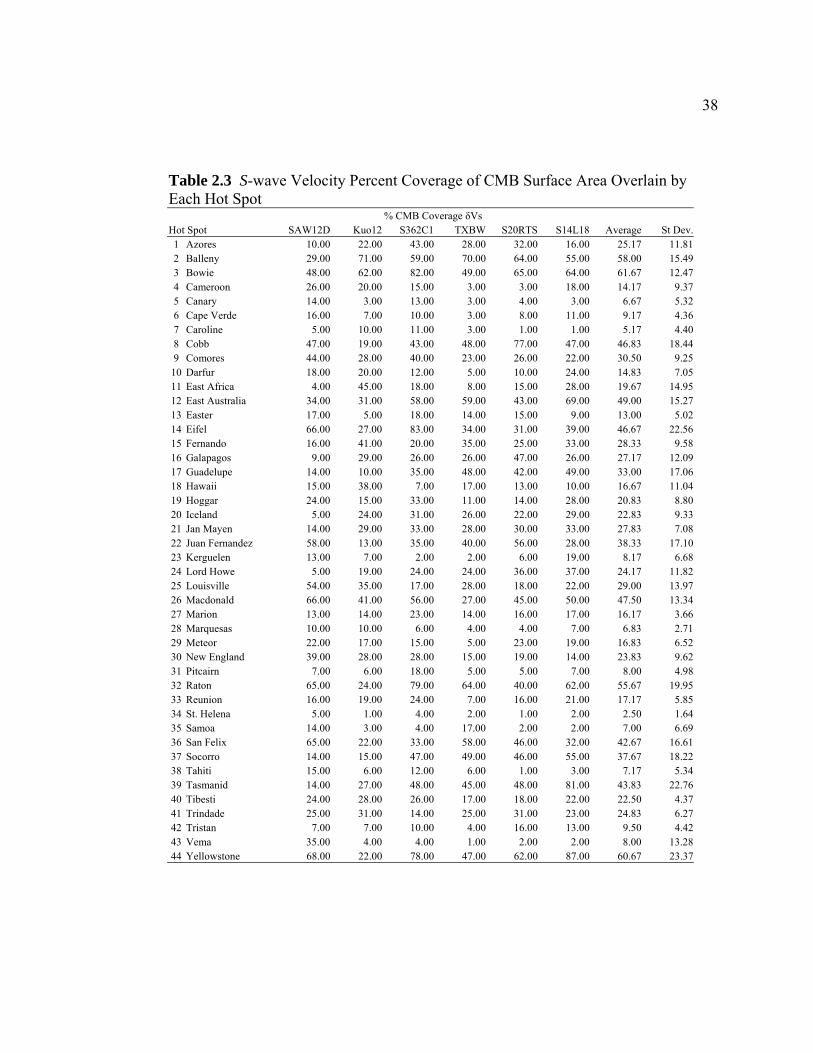
38

Table 2.3 S-wave Velocity Percent Coverage of CMB Surface Area Overlain byEach Hot Spot % CMB Coverage δVs Hot Spot SAW12D Kuo12 S362C1 TXBW S20RTS S14L18 Average St Dev.1 Azores 10.00 22.00 43.00 28.00 32.00 16.00 25.17 11.812 Balleny 29.00 71.00 59.00 70.00 64.00 55.00 58.00 15.493 Bowie 48.00 62.00 82.00 49.00 65.00 64.00 61.67 12.474 Cameroon 26.00 20.00 15.00 3.00 3.00 18.00 14.17 9.375 Canary 14.00 3.00 13.00 3.00 4.00 3.00 6.67 5.326 Cape Verde 16.00 7.00 10.00 3.00 8.00 11.00 9.17 4.367 Caroline 5.00 10.00 11.00 3.00 1.00 1.00 5.17 4.408 Cobb 47.00 19.00 43.00 48.00 77.00 47.00 46.83 18.449 Comores 44.00 28.00 40.00 23.00 26.00 22.00 30.50 9.25

10 Darfur 18.00 20.00 12.00 5.00 10.00 24.00 14.83 7.0511 East Africa 4.00 45.00 18.00 8.00 15.00 28.00 19.67 14.9512 East Australia 34.00 31.00 58.00 59.00 43.00 69.00 49.00 15.2713 Easter 17.00 5.00 18.00 14.00 15.00 9.00 13.00 5.0214 Eifel 66.00 27.00 83.00 34.00 31.00 39.00 46.67 22.5615 Fernando 16.00 41.00 20.00 35.00 25.00 33.00 28.33 9.5816 Galapagos 9.00 29.00 26.00 26.00 47.00 26.00 27.17 12.0917 Guadelupe 14.00 10.00 35.00 48.00 42.00 49.00 33.00 17.0618 Hawaii 15.00 38.00 7.00 17.00 13.00 10.00 16.67 11.0419 Hoggar 24.00 15.00 33.00 11.00 14.00 28.00 20.83 8.8020 Iceland 5.00 24.00 31.00 26.00 22.00 29.00 22.83 9.3321 Jan Mayen 14.00 29.00 33.00 28.00 30.00 33.00 27.83 7.0822 Juan Fernandez 58.00 13.00 35.00 40.00 56.00 28.00 38.33 17.1023 Kerguelen 13.00 7.00 2.00 2.00 6.00 19.00 8.17 6.6824 Lord Howe 5.00 19.00 24.00 24.00 36.00 37.00 24.17 11.8225 Louisville 54.00 35.00 17.00 28.00 18.00 22.00 29.00 13.9726 Macdonald 66.00 41.00 56.00 27.00 45.00 50.00 47.50 13.3427 Marion 13.00 14.00 23.00 14.00 16.00 17.00 16.17 3.6628 Marquesas 10.00 10.00 6.00 4.00 4.00 7.00 6.83 2.7129 Meteor 22.00 17.00 15.00 5.00 23.00 19.00 16.83 6.5230 New England 39.00 28.00 28.00 15.00 19.00 14.00 23.83 9.6231 Pitcairn 7.00 6.00 18.00 5.00 5.00 7.00 8.00 4.9832 Raton 65.00 24.00 79.00 64.00 40.00 62.00 55.67 19.9533 Reunion 16.00 19.00 24.00 7.00 16.00 21.00 17.17 5.8534 St. Helena 5.00 1.00 4.00 2.00 1.00 2.00 2.50 1.6435 Samoa 14.00 3.00 4.00 17.00 2.00 2.00 7.00 6.6936 San Felix 65.00 22.00 33.00 58.00 46.00 32.00 42.67 16.6137 Socorro 14.00 15.00 47.00 49.00 46.00 55.00 37.67 18.2238 Tahiti 15.00 6.00 12.00 6.00 1.00 3.00 7.17 5.3439 Tasmanid 14.00 27.00 48.00 45.00 48.00 81.00 43.83 22.7640 Tibesti 24.00 28.00 26.00 17.00 18.00 22.00 22.50 4.3741 Trindade 25.00 31.00 14.00 25.00 31.00 23.00 24.83 6.2742 Tristan 7.00 7.00 10.00 4.00 16.00 13.00 9.50 4.4243 Vema 35.00 4.00 4.00 1.00 2.00 2.00 8.00 13.2844 Yellowstone 68.00 22.00 78.00 47.00 62.00 87.00 60.67 23.37

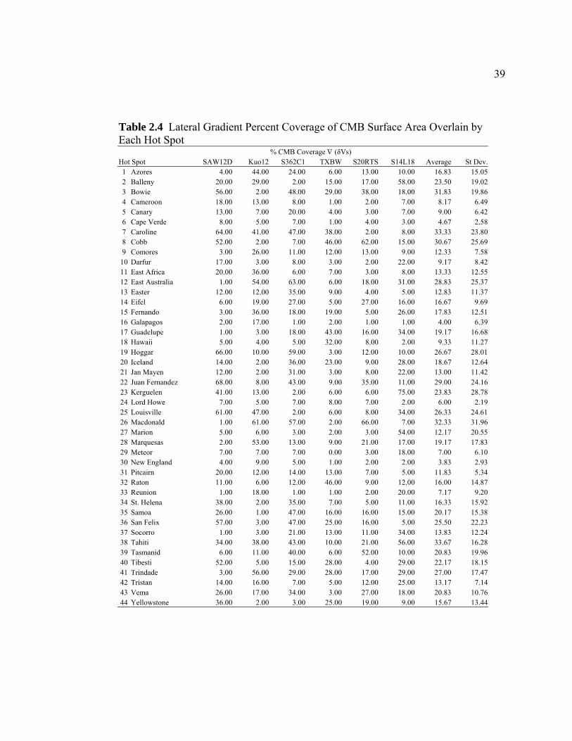
39

Table 2.4 Lateral Gradient Percent Coverage of CMB Surface Area Overlain by Each Hot Spot % CMB Coverage ∇ (δVs) Hot Spot SAW12D Kuo12 S362C1 TXBW S20RTS S14L18 Average St Dev.1 Azores 4.00 44.00 24.00 6.00 13.00 10.00 16.83 15.052 Balleny 20.00 29.00 2.00 15.00 17.00 58.00 23.50 19.023 Bowie 56.00 2.00 48.00 29.00 38.00 18.00 31.83 19.864 Cameroon 18.00 13.00 8.00 1.00 2.00 7.00 8.17 6.495 Canary 13.00 7.00 20.00 4.00 3.00 7.00 9.00 6.426 Cape Verde 8.00 5.00 7.00 1.00 4.00 3.00 4.67 2.587 Caroline 64.00 41.00 47.00 38.00 2.00 8.00 33.33 23.808 Cobb 52.00 2.00 7.00 46.00 62.00 15.00 30.67 25.699 Comores 3.00 26.00 11.00 12.00 13.00 9.00 12.33 7.58

10 Darfur 17.00 3.00 8.00 3.00 2.00 22.00 9.17 8.4211 East Africa 20.00 36.00 6.00 7.00 3.00 8.00 13.33 12.5512 East Australia 1.00 54.00 63.00 6.00 18.00 31.00 28.83 25.3713 Easter 12.00 12.00 35.00 9.00 4.00 5.00 12.83 11.3714 Eifel 6.00 19.00 27.00 5.00 27.00 16.00 16.67 9.6915 Fernando 3.00 36.00 18.00 19.00 5.00 26.00 17.83 12.5116 Galapagos 2.00 17.00 1.00 2.00 1.00 1.00 4.00 6.3917 Guadelupe 1.00 3.00 18.00 43.00 16.00 34.00 19.17 16.6818 Hawaii 5.00 4.00 5.00 32.00 8.00 2.00 9.33 11.2719 Hoggar 66.00 10.00 59.00 3.00 12.00 10.00 26.67 28.0120 Iceland 14.00 2.00 36.00 23.00 9.00 28.00 18.67 12.6421 Jan Mayen 12.00 2.00 31.00 3.00 8.00 22.00 13.00 11.4222 Juan Fernandez 68.00 8.00 43.00 9.00 35.00 11.00 29.00 24.1623 Kerguelen 41.00 13.00 2.00 6.00 6.00 75.00 23.83 28.7824 Lord Howe 7.00 5.00 7.00 8.00 7.00 2.00 6.00 2.1925 Louisville 61.00 47.00 2.00 6.00 8.00 34.00 26.33 24.6126 Macdonald 1.00 61.00 57.00 2.00 66.00 7.00 32.33 31.9627 Marion 5.00 6.00 3.00 2.00 3.00 54.00 12.17 20.5528 Marquesas 2.00 53.00 13.00 9.00 21.00 17.00 19.17 17.8329 Meteor 7.00 7.00 7.00 0.00 3.00 18.00 7.00 6.1030 New England 4.00 9.00 5.00 1.00 2.00 2.00 3.83 2.9331 Pitcairn 20.00 12.00 14.00 13.00 7.00 5.00 11.83 5.3432 Raton 11.00 6.00 12.00 46.00 9.00 12.00 16.00 14.8733 Reunion 1.00 18.00 1.00 1.00 2.00 20.00 7.17 9.2034 St. Helena 38.00 2.00 35.00 7.00 5.00 11.00 16.33 15.9235 Samoa 26.00 1.00 47.00 16.00 16.00 15.00 20.17 15.3836 San Felix 57.00 3.00 47.00 25.00 16.00 5.00 25.50 22.2337 Socorro 1.00 3.00 21.00 13.00 11.00 34.00 13.83 12.2438 Tahiti 34.00 38.00 43.00 10.00 21.00 56.00 33.67 16.2839 Tasmanid 6.00 11.00 40.00 6.00 52.00 10.00 20.83 19.9640 Tibesti 52.00 5.00 15.00 28.00 4.00 29.00 22.17 18.1541 Trindade 3.00 56.00 29.00 28.00 17.00 29.00 27.00 17.4742 Tristan 14.00 16.00 7.00 5.00 12.00 25.00 13.17 7.1443 Vema 26.00 17.00 34.00 3.00 27.00 18.00 20.83 10.7644 Yellowstone 36.00 2.00 3.00 25.00 19.00 9.00 15.67 13.44

40

FIGURES

Figure 2.1 Locations of hot spots used in this study are plotted as closed circles.

Numbers correspond to the number listed next to each hot spot in Tables 2.2, 2.3, and 2.4.

41

42

Figure 2.2 Hot spot counts are shown for model S20RTS. The first column shows

contour lines (green) drawn around 10, 20, and 30% CMB surface area coverage for the

most anomalous low velocities. The second column has contour lines drawn around 10,

20, and 30% CMB surface area coverage for lateral S-wave velocity gradients for a 1000

km arc length with five sample points. The third column shows the CMB percent surface

area coverage, contoured in the first two columns, with lowest velocities filled in red and

strongest gradients filled in green. The surface locations of hot spots are plotted as red

circles. The numbers beneath each drawing show for both S-wave velocity and gradient,

the hot spot count and, in parenthesis, the percentage of the total amount of hot spots and

the percentage of randomly rotated hot spot locations having a weaker correlation within

the CMB percent surface coverage contour. All numbers are obtained using a five-degree

radius bin centered on the hot spot.

43

44

Figure 2.3 The first column displays the raw S-wave velocity perturbations of the six

models analyzed. The second column shows the S-wave velocity models contoured by

surface area coverage of the CMB, where the most anomalous low velocities are

represented by the lowest percentages. The third column shows lateral S-wave velocity

gradients contoured by surface area coverage of the CMB, where the strongest gradients

are represented by the lowest percentages. Lateral velocity gradients shown here are

calculated for a 1000 km length of arc with five sample points used in the least square

approximation. Hot spot surface locations are plotted as red circles in the second and

third columns. Models are as in Table 2.1.

45

Figure 2.4 The number of hot spots falling within the percentage of CMB surface area

coverage are shown for model S20RTS. The triangles show the number of hot spots for a

lateral velocity gradient calculation with a 500 km arc length, while the squares show the

number of hot spots for a gradient calculation with a 1000 km arc length. Both gradient

calculations were done with five points used in the least square approximation. The

circles show the number of hot spots within the percentage of CMB surface area coverage

for velocity.

46

Figure 2.5 The number of hot spots (hot spot hit count and percentage of total amount of

hot spots) that fall within 10, 20, and 30 % CMB surface area coverage for all six S-wave

velocity models. The solid-fill and open-fill symbols show the number of hot spots

falling inside the CMB percent surface area coverage for velocity and lateral S-wave

velocity gradient respectively. Hot spot hit counts are shown using a five-degree radius

bin centered on the hot spot. Gradient calculations were done using a 500 km arc length.

47

Figure 2.6 The standard deviation of the six S-wave models analyzed is shown, where

the magnitude of S-wave velocities are scaled by CMB surface area coverage. The

number of hot spots overlying the ranges of standard deviation 0-10%, 10-20%, and 20-

30% is indicated above the scale-bar. All standard deviation values greater than 30%

(corresponding to < 1% CMB surface area coverage) are shaded the darkest. Hot spots

are drawn as black circles.

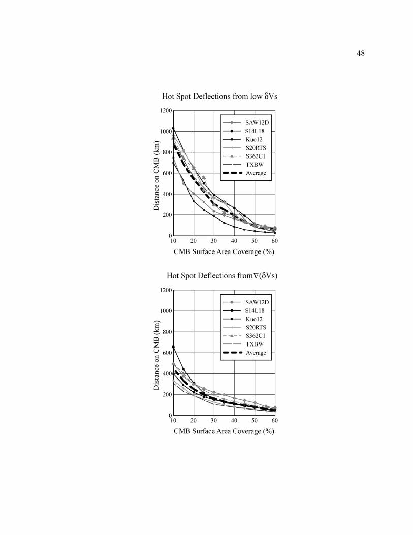
48

49

Figure 2.7 The top panel shows, for each of the six tomographic models analyzed, the

average distance on the CMB for all hot spots to the specified percentage of CMB surface

area coverage for low S-wave velocities. The bottom panel shows the average distance

on the CMB for all hot spots to the specified percentage of CMB surface area coverage

from strong lateral S-wave velocity gradients.

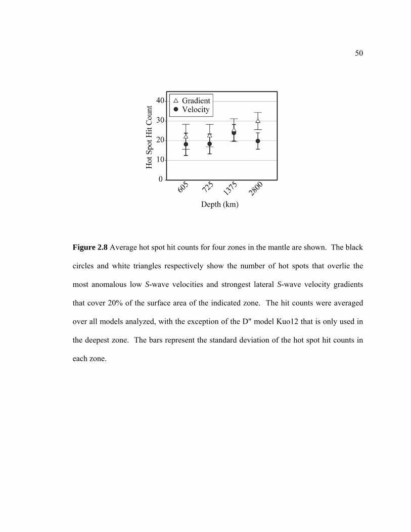
50

Figure 2.8 Average hot spot hit counts for four zones in the mantle are shown. The black

circles and white triangles respectively show the number of hot spots that overlie the

most anomalous low S-wave velocities and strongest lateral S-wave velocity gradients

that cover 20% of the surface area of the indicated zone. The hit counts were averaged

over all models analyzed, with the exception of the D" model Kuo12 that is only used in

the deepest zone. The bars represent the standard deviation of the hot spot hit counts in

each zone.

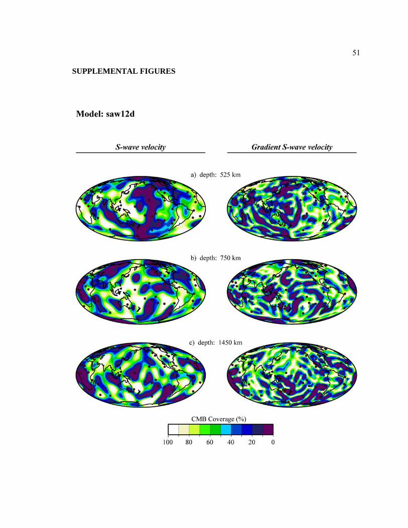
51

SUPPLEMENTAL FIGURES

52

Supplement 2A The first column shows the S-wave velocity model saw12d contoured by

surface area coverage of the CMB, where the most anomalous low velocities are

represented by the lowest percentages. The second column shows lateral S-wave velocity

gradients contoured by surface area coverage of the CMB, where the strongest gradients

are represented by the lowest percentages. Lateral velocity gradients shown here are

calculated for a 1000 km length of arc with five sample points used in the least square

approximation. Hot spot surface locations are plotted as red circles in the second and

third columns. Three depth slices are shown corresponding to depths in the transition

zone, slightly deeper than the transition zone, and the mid-lower mantle. Models are as

in Table 2.1.

53

54

Supplement 2B The first column shows the S-wave velocity model s14l18 contoured by

surface area coverage of the CMB, where the most anomalous low velocities are

represented by the lowest percentages. The second column shows lateral S-wave velocity

gradients contoured by surface area coverage of the CMB, where the strongest gradients

are represented by the lowest percentages. Lateral velocity gradients shown here are

calculated for a 1000 km length of arc with five sample points used in the least square

approximation. Hot spot surface locations are plotted as red circles in the second and

third columns. Three depth slices are shown corresponding to depths in the transition

zone, slightly deeper than the transition zone, and the mid-lower mantle. Models are as

in Table 2.1.

55

56

Supplement 2C The first column shows the S-wave velocity model s20rts contoured by

surface area coverage of the CMB, where the most anomalous low velocities are

represented by the lowest percentages. The second column shows lateral S-wave velocity

gradients contoured by surface area coverage of the CMB, where the strongest gradients

are represented by the lowest percentages. Lateral velocity gradients shown here are

calculated for a 1000 km length of arc with five sample points used in the least square

approximation. Hot spot surface locations are plotted as red circles in the second and

third columns. Three depth slices are shown corresponding to depths in the transition

zone, slightly deeper than the transition zone, and the mid-lower mantle. Models are as

in Table 2.1.

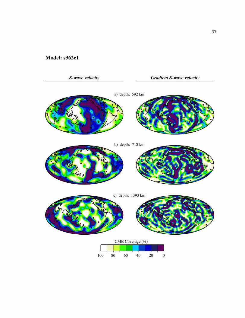
57

58

Supplement 2D The first column shows the S-wave velocity model s362c1 contoured by

surface area coverage of the CMB, where the most anomalous low velocities are

represented by the lowest percentages. The second column shows lateral S-wave velocity

gradients contoured by surface area coverage of the CMB, where the strongest gradients

are represented by the lowest percentages. Lateral velocity gradients shown here are

calculated for a 1000 km length of arc with five sample points used in the least square

approximation. Hot spot surface locations are plotted as red circles in the second and

third columns. Three depth slices are shown corresponding to depths in the transition

zone, slightly deeper than the transition zone, and the mid-lower mantle. Models are as

in Table 2.1.

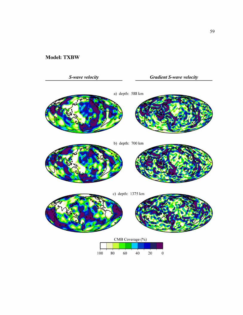
59

60

Supplement 2E The first column shows the S-wave velocity model TXBW contoured by

surface area coverage of the CMB, where the most anomalous low velocities are

represented by the lowest percentages. The second column shows lateral S-wave velocity

gradients contoured by surface area coverage of the CMB, where the strongest gradients

are represented by the lowest percentages. Lateral velocity gradients shown here are

calculated for a 1000 km length of arc with five sample points used in the least square

approximation. Hot spot surface locations are plotted as red circles in the second and

third columns. Three depth slices are shown corresponding to depths in the transition

zone, slightly deeper than the transition zone, and the mid-lower mantle. Models are as

in Table 2.1.

CHAPTER 3

INFERENCES ON ULTRA-LOW VELOCITY ZONE STRUCTURE FROM A

GLOBAL ANALYSIS OF SPdKS WAVES

Michael S. Thorne1 and Edward J. Garnero1

1Dept. of Geological Sciences, Arizona State University, Tempe, AZ 85287, USA

SUMMARY

Anomalous boundary layer structure at the core-mantle boundary (CMB) is investigated

using a global set of broadband SKS and SPdKS waves from permanent and portable

broadband seismometer arrays. SPdKS is an SKS wave that intersects the CMB at the

critical angle for ScP, thus initiating a diffracted P-wave (P ) along the CMB at the core

entry and exit locations. The wave shape and timing of SPdKS data are analyzed relative

to SKS, with some SPdKS data showing significant delays and broadening. Broadband

data from several hundred deep focus earthquakes were analyzed; retaining data with

simple sources and high signal-to-noise ratios resulted in 53 high quality earthquakes.

For each earthquake, an empirical source was constructed by stacking pre-SPdKS

distance range SKS pulses (~90° – 100°). These were utilized in our synthetic modeling

process, whereby reflectivity synthetic seismograms are produced for three classes of

models: (1) mantle-side ultra-low velocity zones (UVLZ), (2) underside-CMB core

rigidity zones (CRZ), and (3) core mantle transition zones (CMTZ). For ULVZ

structures, ratios of P-to-S velocity reductions of 1:1 and 1:3 are explored, where 1:3 is

appropriate for a partial melt origin of ULVZ. Over 330 unique CMB boundary layer

models have been constructed and tested, corroborating previous work suggesting strong

trade-offs between the three model spaces. We produce maps of inferred boundary layer

diff

62

structure from the global data, and find evidence for extremely fine-scale heterogeneity

where our wave path sampling is the densest. While uncertainties are present relating to

the source- versus receiver-sides of the SPdKS wave path geometry, our data are

consistent with the hypothesis that ULVZ presence (or absence) correlates with reduced

(or average) heterogeneity in the overlying mantle.

3.1 Introduction

Evidence for strong P- and S- wave velocity reductions at the core-mantle

boundary (CMB) has been reported for over two decades. Here we briefly summarize

these past efforts, from early CMB heterogeneity and tomography studies to more recent

work specifically aimed at characterization of ultra-low velocity zone (ULVZ) structure,

then discuss the geographic distribution and possible origin of ULVZs presented in past

work. This provides the basis for the work we report in this paper.

3.1.1 Early indirect evidence for ULVZ: CMB topography studies

The first studies reporting strong velocity reductions as well as lateral variations

at the CMB were aimed at resolving CMB topography. For example, models of CMB

topography derived from the inversion of core phases that cross or reflect off of the CMB

(e.g., PKP, PcP) map CMB undulations of up to ± 10 km (e.g., Creager & Jordan 1986;

Morelli & Dziewonski 1987). Additionally, travel time variations of core-reflected PcP

waves referenced to PKP have suggested CMB topography as large as ± 15 km (e.g.,

Rodgers & Wahr 1993). Consensus on the exact distribution or patterns of CMB

63

topography, as well as peak-to-peak topography amplitude, is lacking at present (e.g.,

Rodgers & Wahr 1993; Garcia & Souriau 2000), and subsequent identification of thin

zones of ultra-low velocities further complicate efforts to constrain CMB topography, due

to the strong trade-off between volumetric heterogeneity and CMB topography. Peak-to-

peak amplitudes of CMB topography inferred from seismic studies (up to ±15 km) are

considerably larger than those from dynamical considerations (roughly ±0.5-3 km; e.g.,

see Hager et al. 1985; Bowin 1986; Hide et al. 1993). This discrepancy may in fact be

due to a mismapping of ULVZ signal. We note that the likely existence of CMB

topography does not strongly contaminate ULVZ studies.

Volumetric heterogeneity in the D" region may help reconcile discrepancies in

mapped CMB peak-to-peak amplitudes. By observing the amplitude decay of long-

period Pdiff and Sdiff and short-period Pdiff, Doornbos, (1983) concluded that the CMB

might have significant lateral variations within a relatively thin (<100 km) low velocity

boundary layer. Subsequently, Doornbos and Hilton, (1989) inverted PcP, PKP, and

PnKP for CMB topography to support relatively reduced CMB topography (± 4 km), and

argued that lateral variations in travel time residuals of PcP and PKP can be best

modeled by a laterally varying lowermost mantle boundary layer (in the form of variable

layer thickness, velocity fluctuations, or some combination of the two), with average

layer thickness of ~20 km, and P-wave velocity heterogeneity perturbations up to ±7.3%.

While the thickness of their solution layer is not well constrained because there is a direct

trade-off with velocity heterogeneity in the layer, the inference for thin zones of strong

reductions was made. A recent demonstration of this trade-off arose in a joint inversion

64

for peak-to-peak topography and D" heterogeneity using the seismic phases PcP, PKP,

and PKKP: Sze & van der Hilst (2003) found that ±13 km CMB undulations are

necessary if no D" velocity variations are invoked. This reduces to CMB topography

amplitude of ± 3 km if ± 5% D" variations (lowermost 290 km) in P-wave velocities are

considered. Further evidence for this trade-off was reported by Garcia & Souriau (2000);

they present evidence for peak-to-peak topography from 1.5-4.0 km with lateral scales of

300-1500 km. These recent models are in greater agreement with dynamical models in

terms of peak-to-peak topography values. We note that shorter scale CMB topography or

roughness may be superimposed on this longer wavelength CMB topography (Earle &

Shearer 1997; Shearer et al. 1998; Garcia & Souriau 2000).

A multitude of studies over the last 15-20 years have put forth evidence for strong

deep mantle heterogeneity. These efforts may have similarly mapped ULVZ signal into

larger scale D" heterogeneity. This may be especially relevant for lower mantle structure

from tomographic studies. Currently, the highest resolution modeling efforts have

presented heterogeneity at lateral and vertical scales on the order of 500+ km (e.g.,

Masters et al. 2000; Megnin & Romanowicz 2000; Grand 2002). Small scale ULVZ

structure likely maps into these velocity predictions, though to what extent is extremely

difficult to assess, because it is quite likely that strong D" heterogeneity exists in addition

to ULVZ structure (see, for example, review by Garnero 2000).

65

3.1.2 Recent probes of ULVZ structure

Recent efforts have been aimed at looking directly for ULVZ structure. A

summary of these studies is provided in Table 3.1. The probes used can be organized as

follows: precursors to the core-reflected phases PcP and ScP, scattering from the core

wave PKP, and travel time and/or waveform anomalies of a variety of mantle and core

waves, including ScS, SPdKS, PcP, and PKP.

Analysis of precursors to the core-reflected phases PcP and ScP has proven

extremely valuable in mapping detailed structure of boundary layer structure at the CMB.

These studies have predominantly utilized short-period array data, revealing a wide

variety of observations from a simple CMB with no evident precursors (Vidale & Benz

1992; Castle & van der Hilst 2000), to highly anomalous zones characterized as ULVZ or

thin core-side layering with finite rigidity (a “core-rigidity zone”, or CRZ) with small-

scale lateral variations on the order of 10’s of kilometers (e.g., Garnero & Vidale 1999;

Rost & Revenaugh 2001; Rost & Revenaugh 2003). These studies also highlight

apparent contradictions in some geographic locales where evidence for and against

anomalous boundary layer structure have been put forth. For example, using short-period

PcP stacks, Mori & Helmberger (1995) and Revenaugh & Meyer (1997) both observed

precursors in the Central Pacific that indicated the presence of a ULVZ. However, these

two studies disagree as to whether a ULVZ exists in a location in the East Pacific. The

recent use of broadband data is helping to reconcile these contradictions, as well as better

constrain the limits on sharpness of the structural features responsible for precursors

(Havens & Revenaugh 2001; Rondenay & Fischer 2003).

66

Small scale scatterers in D" can give rise to PKP precursors, and have also been

used to map anomalous ULVZ and CMB structure (e.g., Vidale & Hedlin 1998; Wen &

Helmberger 1998b). PKP precursors attributed to ULVZ structure have been observed in

short-period, long-period, and broadband data (see Table 3.1). The presence of short-

and long-period PKP precursors in data from a given region can be attributed to variable

scatterer scale lengths, from 10’s of km up to 100-300 km (Wen & Helmberger 1998b).

Additionally, migration techniques have been employed to locate scatterers with scale

lengths of ~ 10-50 km (Thomas et al. 1999). The presence of large S-wave velocity

reductions relative to P-wave reductions, as predicted by the partial melt origin of the

ultra-low velocities (Williams & Garnero 1996; Berryman 2000), produces observable

SKS precursors for ULVZ layer thickness greater than ~15 km (if velocity reductions are

10 and 30% for P and S, respectively). However, these have not yet been identified or

documented (Stutzmann et al. 2000). Such precursors would go undetected if either (a)

partial melt layering is thinner than 10-15 km, or (b) the P and S wave reductions are less

than 10 and 30%, respectively, such as 5 and 15% or less.

In addition to studying precursors, a wide variety of studies have inferred ULVZ

presence from differential travel time and waveform anomalies of SPdKS waves

referenced to SKS (Table 3.1). One advantage in using SPdKS is greatly increased global

sampling. However, inherent trade-offs exist in constraining ULVZ elastic parameters as

well as geographic location, which are discussed in detail in this paper. Additionally,

travel-time and waveform studies of ScS relative to S have proven significant in revealing

67

ULVZ structure in regions not sampled by SPdKS (Simmons & Grand 2002; Ni &

Helmberger 2003b).

3.1.3 Geographic distribution of ULVZ

Most ULVZ studies have utilized the abundance of deep focus earthquakes from

the Pacific rim, which has resulted in CMB structure beneath three areas being

extensively studied: 1) the Southwest Pacific, 2) Central America, and 3) the Northeast

Pacific. Figure 3.1 summarizes the results of previous studies under the Southwest

Pacific and Central America regions. The Southwest Pacific region is dominated by a

large low-velocity anomaly prominent in models of shear-wave tomography (e.g., see

Masters et al. 2000), and may also contain the source of several hotspots (e.g., see Sleep

1990; Steinberger 2000; Montelli et al. 2004; Thorne et al. 2004). In contrast to this, the

Central America region may be home to remnants of the subducted Farallon slab as

indicated by relatively high shear-wave velocities (e.g., Grand et al. 1997). Evidence for

a small-scale, high attenuation, low-velocity anomaly has also been put forth for the

Caribbean region (Wysession et al. 2001; Fisher et al. 2003), as well as short scale lateral

heterogeneity (Tkalčić & Romanowicz 2002). Additionally, the source of the Galapagos,

Guadelupe, and Socorro hotspots may lie in the west of this region. Lightly shaded

patches represent SPdKS Fresnel zones: pink denotes ULVZ detection; light blue

indicates that no ULVZ was detected (Garnero et al. 1998). These zones predominantly

characterize long wavelength structure. Shorter scale length ULVZ phenomena are

provided from core reflected precursors or scattering studies: a high degree of variability

68

is observed, as can be seen in the southwest Pacific (symbols, lines, Figure 3.1a). For

example, observations of ScP precursors that indicate anomalous boundary layer

structure are co-located with normal ScP waveforms (Garnero & Vidale 1999; Reasoner

& Revenaugh 2000; Rost & Revenaugh 2001; Rost & Revenaugh 2003). Disagreement

between the long wavelength ULVZ map (Garnero et al. 1998) and the short-scale results

shown in Figure 3.1 are due to (a) ULVZ heterogeneity existing at wavelengths shorter

than SPdKS Fresnel zones, (b) uncertainties due to the source-receiver side ambiguity of

the source of SPdKS anomalies (which we address later in this paper) and (c) possible

sensitivity to different ULVZ structure features.

3.1.4 Origin of ULVZ anomalies

Several explanations have been proposed for the origin of ULVZ structure. These

fall into the categories of (a) chemically unique material on the mantle-side of the CMB

(e.g., Manga & Jeanloz 1996; Stutzmann et al. 2000), (b) partial melt of some component

of the lowermost mantle right at/above the CMB (e.g., Williams & Garnero 1996;

Revenaugh & Meyer 1997; Helmberger et al. 1998; Vidale & Hedlin 1998; Williams et

al. 1998; Zerr et al. 1998; Berryman 2000; Wen 2000), (c) material with finite rigidity

pooling at the underside of the CMB, for example, beneath CMB topographical highs

(e.g., Buffett et al. 2000; Rost & Revenaugh 2001), (d) some form of blurring of the

CMB, such as a transition between core and mantle material from some form of mixing

or chemical reactions (Garnero & Jeanloz 2000a; Garnero & Jeanloz 2000b), and (e) any

combination of the above (Rost & Revenaugh 2001). Increased resolution is necessary

69

for better characterization of boundary layer structure at the CMB. This is additionally

important as it may relate to the source regions of whole mantle plumes responsible for

hotspot volcanism (Williams et al. 1998), the frequency of magnetic field reversals

(Glatzmaier et al. 1999), and nutation of Earth’s rotation axis (Buffett et al. 2000). At a

minimum, the patches or zones of ultra-low velocities are likely related to deep mantle

dynamics and chemistry. To more accurately constrain elastic properties of boundary

layer structure at the CMB, we improve CMB coverage in this paper as sampled by

broadband SPdKS data, which we hope can contribute to future analyses using the

various other probes (e.g., Table 3.1).

3.2 SPdKS Data

This study utilizes a global set of broadband SPdKS data. SPdKS is an SKS wave,

where the down-going S-wave intersects the CMB at the critical angle for diffraction

generating P-diffracted (Pdiff) segments propagating on the mantle-side of the CMB.

The complementary phase SKPdS has the Pdiff leg occurring on the receiver side, where

the up-going P-wave intersects the CMB at the critical angle. For the PREM model

(Dziewonski & Anderson 1981), SPdKS initiates at ~104°, however, the bifurcation

between SKS and SPdKS is not observable in broadband waveforms until ~110°. Ray

path geometries are shown for four distances in the top row of Figure 3.2, with both

SPdKS and SKPdS being displayed. As the source-receiver distance increases, the length

of Pdiff segments on the CMB increases, which is the only alteration to SPdKS+SKPdS

paths with distance. For example, for PREM, Pdiff segments are 420 and 1000 km, for

70

110° and 120° source-receiver distances respectively (see middle row of Figure 3.2). The

distance between the core entry (exit) locations of SKS and SPdKS (SKPdS) at the CMB

also increases with distance. For example, for PREM, the SKS – SPdKS separation

increases from 60 to 210 km for a source-receiver distance increase of 110° to 120° (see

middle row of Figure 3.2). Example synthetic seismograms (for PREM) for the four

distances are shown in the bottom row in Figure 3.2. Data with source-receiver distances

of 110°–115° are most useful as strong waveform distortions are observed, particularly

near 110° where interference with SKS results in diagnostic waveform shapes. Source-

receiver geometries with distances of near 120° (and greater) have broader SPdKS pulses

due to long Pdiff segments. These are less useful for modeling detailed short-scale ULVZ

structure, because CMB and D" structure is averaged over fairly large distances. If the

mantle structure encountered on both the source and receiver side CMB crossing location

is identical, SPdKS and SKPdS have coincident arrival times. However, differing source-

and receiver-side mantle structure should affect the timing, amplitude, and wave shape of

SPdKS and SKPdS (e.g., Rondenay & Fischer 2003). Yet, it is not generally possible to

distinguish SPdKS from SKPdS in observed waveforms. We note one recent array

analysis using the phase stripping method of eigenimage decomposition has been able to

separately identify the source and receiver contributions to the combined wave fields

(Rondenay & Fischer 2003). For convenience, the combined SPdKS plus SKPdS energy

is referred to as SPdKS throughout this paper.

Figure 3.2 also shows the phase SKiKS, which is an SKS wave that reflects off the

inner core boundary (ray path geometry shown in the top row of Figure 3.2). The bottom

71

row of Figure 3.2 shows the SKiKS arrival at four distances. Most notably, for the PREM

model, SKiKS arrives coincident with SPdKS at a distance of ~120° and may interfere

with the SPdKS arrival.

Data used in this study were collected from the publicly available Incorporated

Research Institutions for Seismology Data Management Center (IRIS DMC). Initially,

we conducted a global search for earthquakes using IRIS’s Fast Archive Recovery

Method (FARM) catalog. We searched for earthquakes with depths greater than 100 km,

and moment magnitudes (Mw) greater than 6.0, for events occurring between the years

1990 and 2000. This resulted in a collection of 321 events. To further augment our data

set we also obtained broadband data for several earthquakes from the Observatories and

Research Facilities for European Seismology (ORFEUS) Data Center (ODC), the

Canadian National Seismic Network (CNSN), and PASSCAL data available from the

IRIS DMC.

All data were instrument-deconvolved to displacement using the Seismic Analysis

Code (SAC) (Goldstein et al. 1999) transfer function, and the pole-zero response files

obtained from the IRIS DMC, with a band pass window from 0.01 to 1.0 Hz. Resultant

displacement files were then rotated to great circle path radial and transverse components

and resampled to a 0.1 sec time interval. We retained radial component seismograms, for

analysis of SPdKS relative to SKS.

All data were visually inspected to determine data quality; initial criteria leading

to data rejection were: 1) no stations in the epicentral distance range of 90º to 125º, or 2)

it was not possible to clearly distinguish the seismic phase SKS above the background

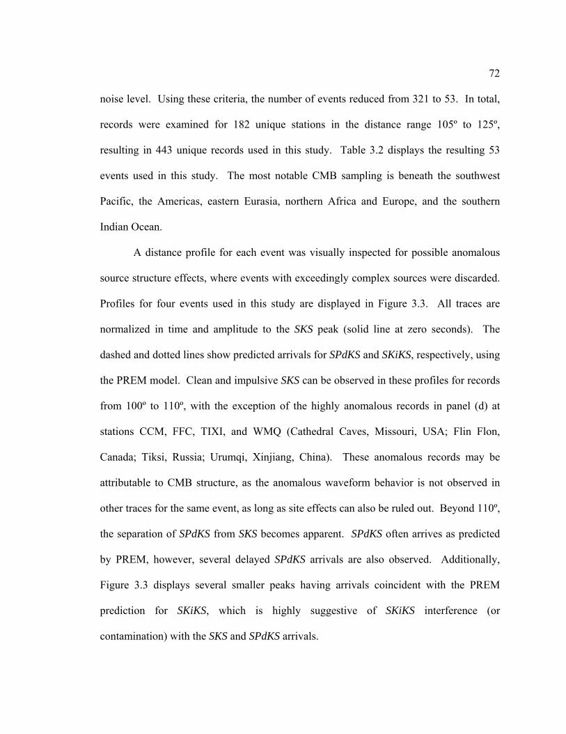
72

noise level. Using these criteria, the number of events reduced from 321 to 53. In total,

records were examined for 182 unique stations in the distance range 105º to 125º,

resulting in 443 unique records used in this study. Table 3.2 displays the resulting 53

events used in this study. The most notable CMB sampling is beneath the southwest

Pacific, the Americas, eastern Eurasia, northern Africa and Europe, and the southern

Indian Ocean.

A distance profile for each event was visually inspected for possible anomalous

source structure effects, where events with exceedingly complex sources were discarded.

Profiles for four events used in this study are displayed in Figure 3.3. All traces are

normalized in time and amplitude to the SKS peak (solid line at zero seconds). The

dashed and dotted lines show predicted arrivals for SPdKS and SKiKS, respectively, using

the PREM model. Clean and impulsive SKS can be observed in these profiles for records

from 100º to 110º, with the exception of the highly anomalous records in panel (d) at

stations CCM, FFC, TIXI, and WMQ (Cathedral Caves, Missouri, USA; Flin Flon,

Canada; Tiksi, Russia; Urumqi, Xinjiang, China). These anomalous records may be

attributable to CMB structure, as the anomalous waveform behavior is not observed in

other traces for the same event, as long as site effects can also be ruled out. Beyond 110º,

the separation of SPdKS from SKS becomes apparent. SPdKS often arrives as predicted

by PREM, however, several delayed SPdKS arrivals are also observed. Additionally,

Figure 3.3 displays several smaller peaks having arrivals coincident with the PREM

prediction for SKiKS, which is highly suggestive of SKiKS interference (or

contamination) with the SKS and SPdKS arrivals.

73

To determine if site effects are contributing to anomalous waveforms, SPdKS

behavior at individual stations has been studied. Figure 3.4 shows distance profiles for

four broadband stations. Three extremely anomalous records are seen for station CCM

around 107º (Figure 3.4a). These anomalous traces show SPdKS (right-shoulder) with

higher amplitudes than SKS (left-shoulder), which is not predicted by the PREM model.

Because other traces at CCM do not show two distinct shoulders, site effects are ruled

out; also, these anomalous effects are not seen for these 3 events at other stations (not

shown), ruling out source mechanism effects.

SKS and SPdKS are extremely close throughout the mantle, except where the Pdiff

segments occur in SPdKS; therefore the source of the anomalous waveforms is attributed

to structure at the CMB, once source mechanism and site effects are ruled out (as

discussed above). Similarly, highly anomalous records can be seen in Figure 3.4b near

112º for station WMQ; again, site effects can be ruled out. One of the anomalous WMQ

records is observed in Figure 3.3d, where several records display anomalous waveforms.

However, most records for that event have an impulsive SKS peak, suggesting that the

anomaly observed at WMQ is likely attributable to CMB structure and not source

mechanism effects. The additional anomalous records seen in Figure 3.3d (CCM, FFC,

SUR) also suggest anomalous CMB structure, somewhere along the Pdiff paths.

3.3 Synthetic seismograms

A large bank of CMB boundary layer models (ULVZ, CRZ, CMTZ) were

constructed for computation of synthetic seismograms to compare to our data, using the

74

1-D reflectivity method (Fuchs & Müller 1971; Müller 1985). Helmberger et al. (1996)

found that the properties of 1-D synthetics were similar to those of 2-D synthetics. The

main drawback in the 1-D approach is that boundary layer modeling cannot address

structure confined to one side of the SPdKS path (i.e., the core entry versus exit location

where Pdiff occurs). Furthermore, using the 1-D approach, we cannot take into account

focusing/defocusing effects of ULVZ or CMB topography, or volumetric heterogeneity,

as can be modeled in 2- or 3-dimensions (e.g., Wen & Helmberger 1998a). Effects of D"

anisotropy are also excluded from modeling in the 1-D case, however we don’t expect

this to affect our data. In addition, the reflectivity method makes use of the Earth

flattening approximation, which may also affect the validity of large distance synthetic

seismograms of core phases in the P-SV system (Choy et al. 1980). Nevertheless, as we

are documenting relative changes in waveform behavior of SPdKS to SKS, we are still

able to document the relative boundary layer anomalies responsible for the waveform

changes by using the 1-D method. Furthermore, documentation of modeling trade-offs is

straightforward, whereas this becomes increasingly difficult with 2-D or 3-D methods

due to the increase in modeling degrees of freedom.

In accordance with proposed models of boundary layer structure at the CMB, we

created synthetic seismograms for CMTZ, CRZ and ULVZ model spaces, using PREM

as the reference model throughout the rest of the Earth. Synthetic seismograms were

produced for a fine discretization in epicentral distance and source depth so every

observation could be compared to predictions from every model. The types of models we

used are summarized in Figure 3.5. We specifically explored variations in boundary

75

layer thickness (“h”, Figure 3.5), P- and S-wave velocity reductions, and density (ρ)

increases; a summary of the ranges explored is given in Table 3.3. For ULVZ structures,

two classes of models were considered: 1) an equal reduction of VP and VS (δVP and δVS

respectively), and 2) δVS equal to three times δVP. The first class of models is

representative of a chemically distinct solid ULVZ, whereas the second corresponds to a

partial melt origin of the ULVZ (Williams & Garnero 1996). For both cases, δVP, δVS, ρ,

and ULVZ thickness were allowed to vary (Figure 3.5a). We created CRZ models by

assuming there is a small finite rigidity at the top of the core. To accommodate this

assumption CRZ models were created by assuming a non-zero value of S-wave velocity

(VS) in the outer core, and rigidity (µ) calculated from µ=ρVS2. This non-zero rigidity

perturbs the outermost core P-wave velocity (VP = [(K + 4/3µ)/ρ]½) in the CRZ, making

it larger than that of PREM (by up to 33%). Hence, with CRZ models, we allowed

thickness, density, and VS to vary, which involve VP perturbations due to finite µ (Figure

3.5b). CMTZ models were created with a linear gradient from lower mantle properties at

the top of the CMTZ layer to outer core properties at the bottom of the CMTZ layer.

CMTZ models are centered in depth on the CMB with layer thickness as the only

variable (Figure 3.5c).

The parameter range for each model space (Table 3.3) was discretized as follows:

for both classes of ULVZ models, ULVZ thickness was modeled as being 2, 5, 10, or 30

km, and lowermost mantle ρ was modeled as a 0, 10, 20, 40, or 60% increase (i.e.,

relative to the PREM mantle). For class 1, equal δVP and δVS reductions ranged from 0,

5, 10, 15, 20, and 30%. For class 2, δVP and δVS reductions of 5 and 15%, 10 and 30%,

76

15 and 45%, or 20 and 60% respectively (i.e., δVS = 3δVP), were tested. This resulted in

200 unique ULVZ models. CRZ models were discretized in 1.0 km thickness

increments, resulting in 4 unique CRZ thicknesses. Additionally, the CRZ layer

contained non-zero VS between 1.0 and 5.0 km/sec in 1.0-km/sec increments, and outer-

core density reductions by up to –50% in 10% increments. Therefore, our CRZ model

space consisted of 4 thicknesses × 5 VS values × 6 ρ reductions, equaling 120 distinct

CRZ models. For CMTZ models, thickness (the only variable) was discretized in 0.25

km increments, resulting in 11 unique models. Thus, our model space consisted of

synthetic seismograms for 333 distinct models that span the range of parameters in Table

3.3. Synthetic seismogram construction for each model for a range of source depths and

distances resulted in nearly 200,000 synthetic seismograms in our model space database

to be compared to data traces.

Previous modeling of ULVZ structure has shown evidence for low quality factor

(Q) values (Havens & Revenaugh 2001), which may be expected if the ULVZ structure is

composed of partial melt. However, in creating this synthetic model space we do not

consider variations in Q. This is primarily an effort to limit the number of parameters,

noting that extremely low Q (e.g., Qµ = 5, QΚ = 5) variations will lower SPdKS

amplitudes but roughly retain relative SKS-SPdKS timing (Garnero & Helmberger 1998).

Nevertheless, future efforts should consider Q, especially for probes that demonstrate a

first-order sensitivity to it.

77

3.4 Modeling approach

In order to compare SPdKS observations to synthetic predictions, we first

constructed an empirical source for each of the events used in this study (Table 3.2). On

an event-by-event basis, SKS pulses were stacked if (a) they were at pre-SPdKS distances

between 90º-100º; (b) they were clean and impulsive; and (c) they had a high degree of

waveform similarity, manifest in a high cross-correlation (CC) coefficient with other

records for that event. Figure 3.6 shows an example empirical source construction, where

24 individual SKS records between 90º-100º (Fig. 3.6a) are summed (Fig. 3.6b) for event

#30 (Table 3.2). The dashed gray line is the resulting linear stack and is shown overlain

on the original 24 traces. For each event, the following steps were carried out to best

incorporate the empirical source in our synthetic modeling: (1) We conducted a

systematic grid search for a triangle function that when convolved with a pre-SPdKS

distance PREM synthetic seismogram returned the best CC coefficient with our empirical

source function (Figure 3.6c, step 3). We created triangle functions by starting with a

delta function, and then alternately varying the right- and left-hand width of the triangle

in 0.1 sec increments, which included both symmetric and asymmetric triangle functions.

Truncated triangle functions were also considered. (2) The best fitting triangle function

was convolved with all synthetic seismograms in our model space. (3) A 45 sec time

window containing SKS and SPdKS for all data and synthetics (at appropriate source

depths and distances) was constructed. Each data record was cross-correlated with the

appropriate depth and distance synthetic seismogram of all of the 333 models. The

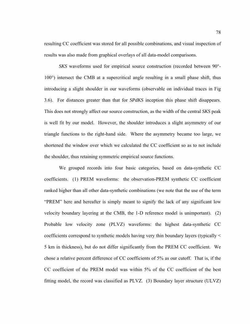
78

resulting CC coefficient was stored for all possible combinations, and visual inspection of

results was also made from graphical overlays of all data-model comparisons.

SKS waveforms used for empirical source construction (recorded between 90°-

100°) intersect the CMB at a supercritical angle resulting in a small phase shift, thus

introducing a slight shoulder in our waveforms (observable on individual traces in Fig

3.6). For distances greater than that for SPdKS inception this phase shift disappears.

This does not strongly affect our source construction, as the width of the central SKS peak

is well fit by our model. However, the shoulder introduces a slight asymmetry of our

triangle functions to the right-hand side. Where the asymmetry became too large, we

shortened the window over which we calculated the CC coefficient so as to not include

the shoulder, thus retaining symmetric empirical source functions.

We grouped records into four basic categories, based on data-synthetic CC

coefficients. (1) PREM waveforms: the observation-PREM synthetic CC coefficient

ranked higher than all other data-synthetic combinations (we note that the use of the term

“PREM” here and hereafter is simply meant to signify the lack of any significant low

velocity boundary layering at the CMB, the 1-D reference model is unimportant). (2)

Probable low velocity zone (PLVZ) waveforms: the highest data-synthetic CC

coefficients correspond to synthetic models having very thin boundary layers (typically <

5 km in thickness), but do not differ significantly from the PREM CC coefficient. We

chose a relative percent difference of CC coefficients of 5% as our cutoff. That is, if the

CC coefficient of the PREM model was within 5% of the CC coefficient of the best

fitting model, the record was classified as PLVZ. (3) Boundary layer structure (ULVZ)

79

waveforms: the highest data-synthetic CC coefficients are from significant CMB

boundary layer model synthetics (hereafter we refer to these waveforms as simply

“ULVZ” although CRZ, or CMTZ models may apply as well). For this case, the PREM

CC coefficient normalized to that of the best fitting model is below 95%. (4) Extreme

waveforms: observations are not adequately fit by any synthetic in our model space –

typically, these waveforms exhibited much higher amplitudes of SPdKS relative to SKS

(as seen in Figure 3.4a, 108º) than are present in any of our models. In some cases this

may be indicative of 2- or 3-D structure causing focusing effects, however, further

investigation is needed in order to explain these records. Records of this class are

assumed to sample an extreme low-velocity zone, or ELVZ. No CC coefficient-based

modeling for ELVZ waveforms is made, due to the high degree of variability of these

records (and subsequent CC coefficients). The lack of a well-defined basis for

classification of ELVZ records does not produce problems in our analyses, as we only

use the ELVZ characterization in searching for spatial groupings of Pdiff segments that

display similar properties, and may elucidate highly anomalous regions of the CMB.

Figure 3.7 shows examples of comparisons between data (bold lines) and

synthetics (thin lines). Figure 3.7(a-c) presents observed waveforms best fit by the PREM

model. Observation-prediction comparisons are shown for PREM along with 11 models

having the next highest cross-correlation coefficient. Cross-correlation coefficients are

displayed to the right of each overlay, and model properties are listed in Table 3.4. Due

to the fine-discretization of the model space (i.e., models span properties that are only

slight perturbations from PREM, up to more extreme ULVZ structures), only a gradual

80

degradation in fit from the best fit PREM prediction is seen. Nonetheless, PREM is the

best fit. For example, Figure 3.7a shows that slight CMB perturbations result in SPdKS

delays relative to SKS, which degrades the CC goodness of fit. Figure 3.7(d-f) shows

examples of the PLVZ observations and predictions. The 11 best fitting synthetics are

overlain on the data, and the 12th overlay is the data and PREM. All waveform

complexities are better reproduced by models with a thin anomalous boundary layer,

though the PREM fit only slightly differs from the fits with higher cross-correlation

coefficients. For example, the best fit-normalized CC coefficient for PREM for Figure

3.7d is 100 × (1 - 96.48/97.13) or ~ 0.7%; these data are thus grouped into the PLVZ

category. Figure 3.7(g,h) shows data and synthetic comparisons for the boundary layer

structure category (ULVZ). The data are fit by significant (> 5% relative difference in

CC coefficients) low velocity CMB layering (contrast with the PREM synthetic at the

bottom of each panel); and Figure 3.7i displays a comparison for the ELVZ waveform

category. This record could not be explained adequately by any of our models

constructed, and was thus grouped into the extreme category.

It is noteworthy that the model giving the highest cross-correlation coefficient

does not necessarily fit the observation the best in terms of SPdKS amplitude and timing.

For example, in Figure 3.7e for station BDFB (Brasilia, Brazil), SPdKS is observed to

arrive slightly later than predicted by the model with the highest CC coefficient. This

SPdKS arrival time may be better predicted by one of the models with a lower ranking

cross-correlation coefficient, however the downswing between SKS and SPdKS is over-

predicted. Furthermore, notable model parameter trade-offs can be seen between models

81

ranked nearly the same in CC coefficient. These 1-D model trade-offs between

thickness, density and velocity variations have been explored in previous work (Garnero

& Helmberger 1998; Garnero & Jeanloz 2000a), and show the difficulty in uniquely

constraining model parameters. Thus, determination of the best model parameters

describing an individual record is difficult and potentially subject to personal bias. This

is a primary motivation for grouping our observations into the previously described four

categories. We note that the CC method is both useful, in that it aids in large data set

processing, and has shortcomings, given that important waveform subtleties are difficult

to address.

In modeling SPdKS observations, additional considerations must also be taken

into account. First, SPdKS waveforms may undergo constructive and destructive

interference with the phase SKiKS that is observable in broadband data. Figure 3.8 shows

PREM synthetics and sample records that may exhibit interference from SKiKS. The

shaded distance range shows the region of maximum potential interference of SKiKS as

predicted by PREM for an event with a 400 km source depth. The distance range

represented by this gray box can shift to greater distances (by 1-2º) with the presence of

low velocity CMB structure. Several traces seem to be affected by this interference as

evidenced by broadened SPdKS arrivals (e.g., near 120º in Figure 3.8b). This

interference further complicates the waveform modeling, and must be considered in

modeling of broadband SPdKS waveforms as in this study.

Finally, the uniqueness of model fit is highly dependent on epicentral distance.

Records from the SPdKS inception distance up to ~112º contain the most diagnostic wave

82

shape distortions, due to SPdKS modulating the peak, shoulder, and downswing of SKS.

Larger distance recordings are more difficult to uniquely constrain, as SPdKS is a longer

period pulse that has sampled a much longer path along the CMB, as well as structure

above the CMB. These records, even in regions known to contain strong CMB

anomalies, often appear PREM-like. This can be observed in Figure 3.7f, for station

CTAO (Charters Towers, Australia) at 123.9º, models with large ULVZ characteristics

do not remarkably vary from PREM (< 5% CC coefficient difference), whereas for

station SSPA (Standing Stone, Pennsylvania, USA) at 112.7º (Figure 3.7g), the boundary

layer models show characteristics of wave-shape distortions that are quite distinguishable

from PREM (> 5% CC coefficient difference).

The dependency of uniqueness-of-fit on epicentral distance is further explored in

Figure 3.9. Most of the SPdKS distance range studied here is densely sampled (Figure

3.9a). The CC coefficient between each observation and PREM was divided by the

cross-correlation coefficient of the best fitting synthetic for that record. This normalized

PREM-data CC coefficient is averaged in 2.5° distance bins and shown in Figure 3.9b.

The error bars represent 1 standard deviation of the mean. In Figure 3.9b, a value of 1

represents the best fit synthetic and PREM being indistinguishable. The bin between

105° and 110° are close to PREM as for most of the global data, SPdKS anomalies are

typically not yet manifested as SKS waveform distortions. Between 110º and 115º,

however, these distortions are easily viewed, and start to degrade the CC coefficient

between data and PREM. The large increase in the standard deviation indicates the

ability to better distinguish between models for this distance range. At larger distances,

83

both the timing and amplitude of SPdKS do not differ that remarkably from PREM,

resulting in the average normalized CC coefficient again approaching the PREM value

(thus, indicating the reduction in ability of the data beyond 115º to strongly constrain

CMB boundary layer structure).

3.5 Inferred ULVZ distribution

3.5.1 Quantifying ULVZ strength and trade-offs

Our synthetic seismogram model space spans three classes of models: ULVZ, CRZ,

and CMTZ (Figure 3.5). Each record (of collected data) was compared to synthetics of

every model in each of these model classes. As mentioned previously (Section 3.4) there

are strong modeling trade-offs between the different model types, particularly for the

larger distance data. And only relatively subtle changes exist between associated CC

coefficients between data and best fit ULVZ, CRZ, or CMTZ synthetics for the larger

distances. This often precludes constraining whether any particular model class best

explains a given record. Nonetheless, it is still possible to characterize how anomalous

data are in a relative sense, by looking at geographical trends in data best fit by PREM

(i.e., normal mantle), probable low velocity zones (PLVZ), or anomalous boundary layer

structure (ULVZ), where we use “ULVZ” to represent moderate ULVZ, CRZ, or CMTZ.

We have thus classified best fitting models of each observation in this fashion: (a)

PREM, (b) PLVZ, (c) ULVZ, and (d) ELVZ. Although, we are not able to constrain

specific boundary layer properties (e.g., layer thickness, density, and velocity

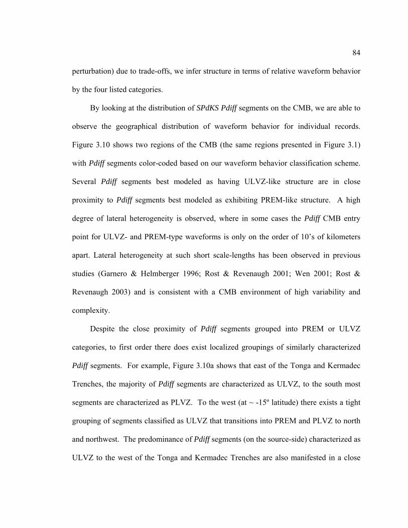
84

perturbation) due to trade-offs, we infer structure in terms of relative waveform behavior

by the four listed categories.

By looking at the distribution of SPdKS Pdiff segments on the CMB, we are able to

observe the geographical distribution of waveform behavior for individual records.

Figure 3.10 shows two regions of the CMB (the same regions presented in Figure 3.1)

with Pdiff segments color-coded based on our waveform behavior classification scheme.

Several Pdiff segments best modeled as having ULVZ-like structure are in close

proximity to Pdiff segments best modeled as exhibiting PREM-like structure. A high

degree of lateral heterogeneity is observed, where in some cases the Pdiff CMB entry

point for ULVZ- and PREM-type waveforms is only on the order of 10’s of kilometers

apart. Lateral heterogeneity at such short scale-lengths has been observed in previous

studies (Garnero & Helmberger 1996; Rost & Revenaugh 2001; Wen 2001; Rost &

Revenaugh 2003) and is consistent with a CMB environment of high variability and

complexity.

Despite the close proximity of Pdiff segments grouped into PREM or ULVZ

categories, to first order there does exist localized groupings of similarly characterized

Pdiff segments. For example, Figure 3.10a shows that east of the Tonga and Kermadec

Trenches, the majority of Pdiff segments are characterized as ULVZ, to the south most

segments are characterized as PLVZ. To the west (at ~ -15º latitude) there exists a tight

grouping of segments classified as ULVZ that transitions into PREM and PLVZ to north

and northwest. The predominance of Pdiff segments (on the source-side) characterized as

ULVZ to the west of the Tonga and Kermadec Trenches are also manifested in a close

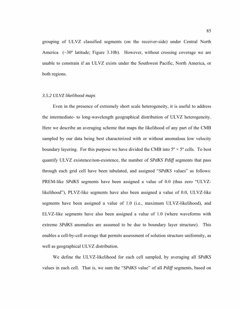
85

grouping of ULVZ classified segments (on the receiver-side) under Central North

America (~30º latitude; Figure 3.10b). However, without crossing coverage we are

unable to constrain if an ULVZ exists under the Southwest Pacific, North America, or

both regions.

3.5.2 ULVZ likelihood maps

Even in the presence of extremely short scale heterogeneity, it is useful to address

the intermediate- to long-wavelength geographical distribution of ULVZ heterogeneity.

Here we describe an averaging scheme that maps the likelihood of any part of the CMB

sampled by our data being best characterized with or without anomalous low velocity

boundary layering. For this purpose we have divided the CMB into 5º × 5º cells. To best

quantify ULVZ existence/non-existence, the number of SPdKS Pdiff segments that pass

through each grid cell have been tabulated, and assigned “SPdKS values” as follows:

PREM-like SPdKS segments have been assigned a value of 0.0 (thus zero “ULVZ-

likelihood”), PLVZ-like segments have also been assigned a value of 0.0, ULVZ-like

segments have been assigned a value of 1.0 (i.e., maximum ULVZ-likelihood), and

ELVZ-like segments have also been assigned a value of 1.0 (where waveforms with

extreme SPdKS anomalies are assumed to be due to boundary layer structure). This

enables a cell-by-cell average that permits assessment of solution structure uniformity, as

well as geographical ULVZ distribution.

We define the ULVZ-likelihood for each cell sampled, by averaging all SPdKS

values in each cell. That is, we sum the “SPdKS value” of all Pdiff segments, based on

86

PREM predicted ray paths, passing through one of our 5º × 5º cells, and weight the sum

by the total number of rays that passed through the cell. If all SPdKS Pdiff segments

passing through a given cell were classified as ULVZ-like, then its ULVZ-likelihood

would correspond to 1.0. If all data were classified as PREM-like, its ULVZ-likelihood

would correspond to 0.0. Figure 3.11 shows the resulting ULVZ likelihood for our

SPdKS data set. Figure 3.12a shows our entire data set with PREM predicted source- and

receiver-side Pdiff segments colored red and blue respectively. In section 3.4 we noted

that records in the epicentral distance range between 110º and 115º provide the greatest

uniqueness of fit (Figure 3.9). For longer source-receiver distances the uniqueness of fit

degrades. Figure 3.11b shows our data coverage for each 5º × 5º cell for our most

distinctive data (restricted between 110º and 120º), where we have colored each grid cell

by the number of Pdiff segments passing through a cell, and Figure 3.11c shows the

ULVZ-likelihood for this restricted range.

When comparing this ULVZ likelihood map (Figure 3.11c) with a comparable

likelihood map utilizing all data (available as additional supplementary information from

the JGR website1) the two ULVZ likelihood maps critically depend on how uniquely

SKS-SPdKS waveform characteristics can reveal CMB structure. While both maps agree

with each other to first-order at long wavelength, distinct differences exist for some

regions. Restricting the distance range has enhanced ULVZ likelihood in many regions,

1 Supporting material is available via Web browser or via Anonymous FTP from ftp://ftp.agu.org/apend/ (Username = “anonymous”, Password = “guest”); subdirectories in the ftp site are arranged by journal and paper number. Information on searching and submitting electronic supplements is found at http://ww.agu.org/pubs/esupp_about.html.

87

by discarding the longest distance (poorly constrained) PREM-fit data. We consider the

first map (Figure 3.11c) to be the more constrained estimation of ULVZ likelihood.

The ULVZ likelihood maps reveal regional scale ULVZ patterns. For example, the

southwest Pacific region and Central American region show high ULVZ likelihood.

Strong ULVZ likelihood is observed under the Indian Ocean although we do not have

complete coverage here. On the other hand, the Central East Asia region is extremely

well sampled and shows no ULVZ likelihood. The central and eastern African CMB

region also shows lesser likelihood of ULVZ, although we note that this is not well

sampled. The area beneath (and west of) Kamchatka displays evidence for ULVZ

existence, which is a region where no ULVZ has previously been observed. Other

regions, such as the area east of the Philippines, are dominated by moderate to low ULVZ

likelihood (midway between ULVZ and PREM). These regions likely contain a high

degree of heterogeneity as suggested by the multiple Pdiff segments of varying

classifications passing through each cell (also see Figure 3.10).

Many studies have focused on the Southwest Pacific and Central American regions

(Figure 3.1, Table 3.1). The Southwest Pacific region has displayed compelling evidence

for ULVZs utilizing varied approaches. To the west and northwest of the Tonga and

Kermadec Trenches, short scale-length heterogeneity has been argued in studies utilizing

short-period precursors to the phase ScP (studies 5,7,10 and 11 in Table 3.1 and Figure

3.1). These studies show ScP bounce points located within 10’s of km on the CMB

displaying waveforms indicative of both existence and non-existence of ULVZ structure.

Our study also shows this high degree of lateral heterogeneity in these regions, with

88

ULVZ likelihood in the range of 0.5 to 0.8 (Figure 3.11c). Studies focusing west of the

Tonga and Kermadec Trenches have agreed on positive ULVZ sighting. This region also

contains some of our highest ULVZ likelihood values. Yet, we also observe intermingled

PREM- and PLVZ- like waveforms suggesting that this region is more complicated than

previously suggested. A variety of results have emerged from studies looking at the

Central American Region. Nearly all of our data for this region displays either ULVZ or

PLVZ-like waveforms. Of special note is the tight grouping of ULVZ- and ELVZ- like

waveforms just to the east of the Galapagos Islands supporting the findings of studies 4

and 18 (Table 3.1, Figure 3.1).

Several studies have searched for ULVZ structures in regions not encompassed in

Figure 3.1. The Northeast Pacific region has received much attention from studies of

short-period precursors to core reflected phases (see Table 3.1), although the majority of

these studies have not shown any evidence of ULVZ structure. Our likelihood map is in

agreement with no ULVZ under the Northeast Pacific, however we only sparsely sample

this region. Wen, (2001) studied the southern Indian Ocean using travel times and

waveform analysis of S, ScS, SHdiff and Pdiff from four events, and found a trend of

PREM-like lowermost mantle in the south to ULVZ-like structure in the north. This

finding coincides remarkably well with the likelihood transition at the southeast tip of

Africa for our most constrainable data (Figure 3.11c). Here we only use data from one of

the four events used by Wen (2001). Additionally, Helmberger et al. (2000) suggests that

ULVZ structure exists beneath Iceland and the East Africa Rift. Our averaging scheme

does not result in the highest ULVZ likelihood (1.0) in either region, but is > 0.5 under

89

Iceland and displays some evidence under the East Africa Rift corroborating this

possibility. However, as noted above, our data coverage is sparse beneath most of Africa.

Further evidence has been supplied that ULVZ structure exists under the Southern

Atlantic Ocean from studies of S-ScS travel times and waveform anomalies (Simmons &

Grand 2002; Ni & Helmberger 2003b). However, we have no data coverage there.

As noted, seemingly conflicting results have been reported for the existence/non-

existence of ULVZs for a given region. The ULVZ-likelihood approach is useful for

identifying regions that display variability in solution models, that often depend on the

wavelength of the energy modeled (e.g., short-period versus broadband data). We stress

that the exact sampling location and dominant wavelength of observation is extremely

important for model determination. The likelihood map presented in Figure 3.11

provides a better estimation of where ULVZ structure may exist than the simple binary

distributions previously presented (e.g., Garnero et al. 1998).

Fresnel zones of the Pdiff segments of SPdKS can also be used in ULVZ map

construction (Garnero et al. 1998). Figure 3.12 shows SPdKS Pdiff Fresnel zones (¼

wavelength, 10 sec dominant period, calculated for a ULVZ model with a 10% reduction

in VP), where the shading represents ULVZ likelihood (as in Figure 3.11). Light shading

corresponds to high likelihood of having ULVZ structure and dark shading indicates low

likelihood. While using Fresnel zones are extremely useful for accommodating likely

wavelengths of wave field sensitivity, caution must be taken in subsequent interpretation,

because significant sub-Fresnel zone variability exists (Figure 3.10). This was a pitfall of

the final ULVZ distribution figure of Garnero et al. (1998) that utilized Fresnel zones –

90

as with Figure 3.12, and the spatial averaging used in Figure 3.11 – lateral variations in

boundary layer structure appears to exist at wavelengths much shorter than Fresnel zones

or our grid cell sizes.

3.6 Discussion

In this paper, we present a method to assign best fit 1-D models to high quality

broadband SPdKS data. Our main focus has been to identify likely regions of anomalous

CMB structure. While this data set and method greatly improve our earlier efforts,

several uncertainties are still present. In this section we discuss important sources of

uncertainty and the relationship between likely ULVZ presence and overlying mantle

heterogeneity.

3.6.1 Uncertainties in mapping ULVZ structure

Perhaps the most significant uncertainty associated with SPdKS analyses is the

difficulty in attributing anomalous SPdKS signals to either the SPdKS core entry or exit

(or both) locations. This is identical to trade-offs in PKP precursor analyses aimed at D"

scatterer modeling (e.g., Hedlin & Shearer 2000). Some crossing paths help to reduce

these uncertainties, but many regions lack any azimuthal sampling.

While static displacements of the CMB do not affect our results, small-scale

topography (e.g., domes, etc.) can act to focus or defocus energy and may play a

significant role in perturbing SPdKS relative to SKS (or vice versa), resulting in erroneous

mapping of structure. Data coverage at present is not adequate to address this issue

91

globally. Some regional efforts (as in Wen & Helmberger 1998a) may have dense

enough sampling to constrain such features.

In most SPdKS modeling to date, synthetic predictions assume that SKS also

propagates through the ULVZ structure, resulting in an SKS delay. For example, a 20 km

thick ULVZ with a 10% δVP reduction results in an SKS delay of ~0.3 sec. In 1-D

modeling, SKS travels through the ULVZ structure twice, thus a 0.6 sec anomaly

accumulates. If in fact SKS does not traverse any ULVZ, then a 0.6 sec bias has been

folded into the modeling, which amounts to an underestimation of SPdKS delays

(because SKS has been artificially delayed, and SPdKS is analyzed relative to SKS). This

affect should only minimally affect our results, because (a) most of our best fit models

are thinner than this example, and (b) a 0.6 sec differential time error will only result in a

minor mismapping of ULVZ strength. Nonetheless, future efforts need to focus beyond

1-D methods.

Our modeling has assumed constant anomalous property layering (except the

CMTZ models), for a single layer. More recent work has suggested multiple ULVZ

layers in two localized regions: beneath the central Pacific (Avants et al. 2003), and

beneath North America (Rondenay & Fischer 2003). Some of our regions may entail

much greater complexity than this first effort at global ULVZ characterization.

Because of the various modeling trade-offs, the absolute velocity reductions,

density increases, or thickness cannot be constrained in this study. However, average

ULVZ properties (e.g., thickness) can be pursued for specific model assumptions. Table

3.5 presents the average ULVZ thickness for a variety of model types. For each model,

92

we: (1) extracted the best fitting thickness of that model type for every SPdKS

observation; (2) discarded records having a CC coefficient (for that specific model)

below 5% of that of the overall best fit synthetic to that observation; and (3) averaged the

resulting thicknesses for all records that fulfilled requirement (2) (this was done

separately for both PLVZ and ULVZ model characterizations). The average thickness is

given in Table 3.5 with the number of qualifying records listed in parenthesis to the right.

It is notable that the number of qualifying records for each of the models presented is

approximately equal (for either PLVZ or ULVZ), which is further indication of the

modeling trade-offs. Nonetheless, several key generalizations can be made from these

modeling summaries:

I. For ULVZ models:

• Doubling the velocity reduction (where δVS = δVP) results in an average ULVZ

thickness roughly halved.

• Doubling the density increase reduces ULVZ thickness by roughly 20%.

• Equal δVS and δVP reductions have the greatest average ULVZ thickness (for the

parameter space we explored with δVS = δVP).

• For δVS = 3δVP (representing the partial melt scenario), greater thicknesses can be

achieved if the velocity reductions are relatively mild. In our model space, the thickest

partially molten ULVZ (~ 8 km) occurs for (δVS = -15%, δVP = -5%, δρ= +0%).

• Increasing velocity reductions or density increases for δVS = 3δVP, the average

ULVZ thickness significantly decreases, e.g., < 5 km average thickness results for (δVS =

-30%, δVP = -10%, δρ = +0%).

93

II. For CRZ models:

• Increasing VS or ρ decreases CRZ thickness.

III. For CMTZ models:

• The average thickness is less than 2.0 km.

If we assume a specific model type (e.g., as in Table 3.5), boundary layer distribution and

thickness maps can be constructed. Figure 3.11d shows the average thickness of one

ULVZ model (δVS = -15%, δVP = -5%, δρ = +5%), averaged onto 5º×5º grid cells.

Additionally, Figures 3.11e,f show the average thickness of one CRZ model (δVS = -

59%, δVP = -34%, δρ = +42%), and for CMTZ. These maps are produced by averaging

best fitting thicknesses in each grid cell, for all data characterized by a CC coefficient

within 5% of the best fitting record (for that specific model). This figure does not include

thickness averages for waveforms classified as PLVZ, and thus represents a maximum

thickness for the sampled regions. Interestingly, thick ULVZ is exhibited (Figure 3.11d)

in the East African Rift Area and under Iceland, as suggested by Helmberger et al.

(2000), where only moderate ULVZ likelihood was suggested (Figure 3.11c).

Approximate thicknesses for other ULVZ model properties may be estimated to first

order from the present map, and Table 3.5. For example, for an ULVZ model with δVS =

-30%, δVP = -10%, and δρ = +0%, the average thickness of each cell would be reduced

by approximately half. We note that our complete list of model parameters, cross-

correlation coefficients, and ULVZ likelihood maps, are available in ASCII format as

additional supplementary information from the JGR website.

94

3.6.2 Relating ULVZ and mantle heterogeneity

We have compared these likelihood maps to several P- and S-wave tomography

models (Boschi & Dziewonski 1999; Megnin & Romanowicz 2000; Ritsema & van

Heijst 2000; Gu et al. 2001; Kárason & van der Hilst 2001; Zhao 2001; Grand 2002).

However, there is no significant correlation between strong ULVZ-likelihood and

lowermost mantle velocities from these tomographic models. This may be expected due

to the source-receiver ambiguity of SPdKS. For example, tomographic models of shear-

wave velocity display strong degree-2 heterogeneity, with low velocities below the

Pacific and Africa, and high velocities in the circum-Pacific region. All of our records

originate in sources along deep subduction zones circling the Pacific. For example, a

record originating in the Fiji-Tonga subduction complex and recorded in North America

or Asia may have Pdiff segments on the source-side encountering low shear-wave

velocities in the Pacific and high shear-wave velocities on the receiver-side in the North

American or Asian regions. Because we cannot distinguish between source- or receiver-

side ULVZ anomalies, ULVZ likelihood estimations in both locales are affected. This

causes an averaging effect in comparing likelihood to tomography results. Thus, while

ULVZ structure may strongly relate to lowermost mantle velocities, the correlation

between our likelihood maps and lowermost mantle velocities may be blurred due to the

source– versus receiver-side of path ambiguity (which is explored in greater detail in the

following section). As data coverage and crossing path sampling increases, future efforts

will better minimize uncertainties due to the source receiver ambiguity in SPdKS

modeling.

95

However, there is a correlation with tomographic models of shear-wave velocity

and the source-side Pdiff segments used in this study. For each record in our study we

have determined the lowest velocity encountered on each Pdiff segment for both source-

and receiver-side arcs, for four models of S-wave tomography (Megnin & Romanowicz

2000; Ritsema & van Heijst 2000; Gu et al. 2001; Grand 2002) and three models of P-

wave tomography (Boschi & Dziewonski 1999; Kárason & van der Hilst 2001; Zhao

2001). The most notable correlation occurs for Pdiff segments from data in the distance

range of 110º–120º. Figure 3.13 shows averages of the lowest tomographic velocities

along either source- or receiver-side Pdiff segments, for the different model

classifications of PREM, PLVZ, or ULVZ (ELVZ waveforms are combined with the

ULVZ waveforms for this analysis). For both the P- and S-wave models, the lowest

velocities encountered by the SPdKS Pdiff segments are predominantly on the source-side

and approximately zero on the receiver side of the path. No clear trend is found between

average P-wave velocities and SPdKS anomalies (i.e., PREM, PLVZ, or ULVZ data),

with the exception of model kh2000pc (Kárason & van der Hilst 2001). For model

kh2000pc, the Pdiff segments on the source-side typically encounter higher velocities for

PREM than for PLVZ (slightly lower), and for ULVZ (lower yet), than for the receiver-

side of the path. This trend is apparent for all S-wave models analyzed. That is,

considering the source-side segments for all S-wave models, the PREM-like waveforms

encounter the higher velocities on average than those classified as ULVZ. Also, PLVZ-

classified waveforms on average encounter S-wave velocities in-between PREM and

96

ULVZ data. The velocity averages for receiver-side Pdiff segments do not show any

apparent trend relating to our waveform classification.

As our inferred structure varies on rather small length-scales, we have attempted

to make our comparisons with global structures with the shortest wavelength variations.

However, no apparent agreement in correlation is evident in the P-wave models, which

may be related to the general disagreement between the models, and indicate a necessity

to utilize models specifically aimed at determining D" structure or at more detailed

regional maps (e.g., Valenzuela et al. 2000, Tkalčić et al. 2002, Tkalčić & Romanowicz

2002). Of the P-wave models analyzed here, only kh2000pc utilizes Pdiff, which may

result in the better correlation to the ULVZ results than for the other P structures. As

longer distance records may inappropriately be classified as PREM-like (see Section

3.5.2), correspondence of low tomographically derived VS and source-side Pdiff arcs is

less apparent when using our entire data set (in comparison to using the 110°-120°

subset). As expected, more PREM-like averages of tomographic velocities encountered

result from inclusion of the largest distance data (i.e., > 120°). Because the main source

region of events used in this study lie in the Southwest Pacific, and the majority of

receiver locations are in Eastern Asia and North America (Figure 3.11a) rays from the

same event are more likely to sample bins on the source-side, whereas bins nearest the

receiver-side are more likely to be sampled by rays from a wide range of events. Hence

the limited coverage enforced by source-receiver geometry inadequacy may introduce a

geographical bias in our low VS and source-side Pdiff arc correspondence.

97

3.6.3 SPdKS ray path uncertainties

In our one-dimensional modeling efforts, boundary layer structure exists at both

the source and receiver sides of the SPdKS path. But, ULVZ structure may be confined

to only one side, and may only partially interact with the Pdiff segments on that side.

Figure 3.14 illustrates three different ULVZ localizations on the source-side. In panel

(a), the SPdKS Pdiff segment initiates, propagates, then exits completely within the

ULVZ (solid line ray path). For reference, the dotted line indicates the ray path for

PREM. Of first note, the critical angle for ScP converting to a Pdiff segment increases

for a ULVZ, as compared to that for PREM . All diffracted waves within a ULVZ exit

into the core at the same model dependent critical angle. The Pdiff inception location

(i.e., where P-diffraction initiates) is closer to the earthquake source for the ULVZ model

than for PREM, resulting in longer diffraction distances (to reach the same receiver).

Panel (b) depicts the situation where Pdiff initiates in PREM mantle, then

propagates in a ULVZ before diving into the core. In this case, the diffraction length is

larger than for pure PREM paths. The opposite geometry is also possible, that is, the Pdiff

inception can occur in an isolated ULVZ, exit the ULVZ into PREM-like mantle, and

then dive into the core from PREM mantle. It is also possible the Pdiff passes through

one or several ULVZ structures of a much smaller scale than the Pdiff arcs. In this case,

travel time anomalies associated with SPdKS may be abrogated by wavefront healing

making their existence difficult to establish.

98

3.6.4 2- and 3-D synthetics

In the three cases of Figure 3.14, the length of diffraction, as well as the Pdiff

inception and termination locations vary significantly. Synthetic waveforms that account

for structure in two- or three-dimensions are desired (e.g., by utilizing methods such as

presented in Igel & Weber 1996; Helmberger et al. 1996; Wen & Helmberger 1998).

Helmberger et al. (1996) studied the effects of two-sided structures, with PREM-like

mantle on one side and a ULVZ structure on the opposite side of the SPdKS path. Two

distinct waveform effects (relative to 1-D modeling) were noticed: (1) a decrease in

SPdKS amplitude near 110°-112° occurs, as the anomalous signal comes from only half

of the geometric path, and (2) at larger distances, two distinct arrivals are apparent, one

for SPdKS and SKPdS. The source versus receiver side of path ambiguity is nevertheless

still present.

3.6.5 Other considerations

A significant amount of waveforms have been characterized as PLVZ, which

raises the possibility that a thin (< 5 km) ULVZ structure may exist throughout much of

Earth’s D" layer. Williams & Garnero (1996) suggested that if ULVZs are of partial melt

origin, they might arise if the geotherm is close to the solidus of silicate mantle. For this

case, ULVZs should be a global feature (as the CMB should be isothermal), but could be

very thin in colder regions. At present it may be difficult to detect such a possibility.

Even with array methods, it is difficult to resolve “typical” ULVZ boundary layering

(e.g., δVS = δVP = –10%) much thinner than ~3 km (e.g., Rost & Revenaugh 2003). A

99

gradational top to the ULVZ may further hinder ULVZ detection in such studies.

However, one may expect greater SPdKS delays in higher frequency data as Pdiff may be

more efficiently trapped inside a ULVZ. Thus, using shorter-period data may prove

useful in future characterizations of ULVZ structure.

As global coverage increases, particularly through combining results of the other

important ULVZ probes, comparisons between better constrained global ULVZ maps and

other related phenomena will be important, such as possible preferred magnetic field

reversal paths (e.g., Laj et al. 1991; Brito et al. 1999; Kutzner & Christensen 2004), or

the geographic distribution of hotspots (e.g., Williams et al. 1998a).

3.7 Conclusions

We have investigated anomalous boundary layer structure at the core-mantle

boundary using a global set of broadband SKS and SPdKS waves. In attempt to

circumvent the strong modeling trade-offs we have produced ULVZ likelihood maps,

inferring regional patterns in ULVZ structure. The Southwest Pacific, Central America,

Indian Ocean and Northeast Asia regions indicate the highest likelihood of ULVZ

existence, whereas the North America, Central East Asia, and Africa regions display the

lowest likelihood. Although there exists ambiguity over whether anomalous boundary

layer structure exists on the source- or receiver-side of the SPdKS paths, there exists an

apparent correlation with lower mantle S-wave velocity as inferred from tomography.

This finding is consistent with ULVZ structure predominantly existing on the source-side

of SPdKS paths. Additionally, broadband SPdKS data is determined to be most sensitive

100

to boundary layer structure in the distance range of 110º-115º. We observe very short-

scale heterogeneity, with Pdiff segments separated by 10’s of kilometers, consistent with

past studies. A partial melt origin to ULVZs implies a global average ULVZ thickness of

< 10 km for δVS = -15%, δVP = -5%, and δρ = +0%. Stronger velocity reductions or

density increases results in an even thinner ULVZ. Better constraint on structural

specifics is necessary; combining SPdKS analyses with other ULVZ probes (both short-

period and broadband) in addition to modeling waveforms with higher dimensional

methods will greatly advance our ability to constrain ULVZ layer properties and

geographical distribution (including the possibility of an ubiquitous ULVZ layer).

ACKNOWLEDGEMENTS

The authors thank T. Lay and S. Rost for useful discussions, the IRIS, ORPHEUS, and

CNSN data agencies for the broadband data, and M. Fouch for helping with data

processing. The authors also thank J. Revenaugh, S. Rondenay, and H. Tkalčić for

constructive review and suggestions. MT and EG were partially supported by NSF grants

EAR-9905710, and EAR-0135119. Most figures were generated using the Generic

Mapping Tools freeware package (Wessel & Smith 1998). Actual waveform data used in

this study is available at http://ulvz.asu.edu

101

REFERENCES

Avants, M.S., T. Lay, & E. Garnero, 2003. Determining shear velocity structure of

ULVZs using stacked ScS data, EOS Trans. AGU, 84 (46). Berryman, J.G., 2000 Seismic velocity decrement ratios for regions of partial melt in the

lower mantle, Geophys. Res. Lett., 27 (3), 421-424. Boschi, L., & A.M. Dziewonski, 1999. High- and low-resolution images of the Earth's

mantle: Implications of different approaches to tomographic modeling, J. Geophys. Res.-Solid Earth, 104 (B11), 25567-25594.

Bowers, D., D.A. McCormack, & D.S. Sharrock, 2000. Observations of PKP(DF) and

PKP(BC) across the United Kingdom: implications for studies of attenuation in the Earth's core, Geophys. J. Int., 140 (2), 374-384.

Bowin, C., 1986 Topography at the Core Mantle Boundary, Geophys. Res. Lett., 13 (13),

1513-1516. Brito, D., J. Aurnou, & P. Olson, 1999. Can heterogeneous core-mantle electromagnetic

coupling control geomagnetic reversals?, Phys. Earth Planet. Inter., 112 (3-4), 159-170.

Buffett, B.A., E.J. Garnero, & R. Jeanloz, 2000. Sediments at the top of Earth's core,

Science, 290 (5495), 1338-1342. Castle, J.C., & R.D. van der Hilst, 2000. The core-mantle boundary under the Gulf of

Alaska: No ULVZ for shear waves, Earth Planet. Sci. Lett., 176 (3-4), 311-321. Choy, G.L., V.F. Cormier, R. Kind, G. Muller, & P.G. Richards, 1980. A Comparison of

Synthetic Seismograms of Core Phases Generated by the Full-Wave Theory and by the Reflectivity Method, Geophysical Journal of the Royal Astronomical Society, 61 (1), 21-39.

Creager, K.C., & T.H. Jordan, 1986. Aspherical Structure of the Core-Mantle Boundary

from PKP Travel-Times, Geophys. Res. Lett., 13 (13), 1497-1500. Doornbos, D.J., 1983 Present Seismic Evidence for a Boundary-Layer at the Base of the

Mantle, Journal of Geophysical Research, 88 (B4), 3498-3505. Doornbos, D.J., & T. Hilton, 1989. Models of the Core-Mantle Boundary and the Travel-

Times of Internally Reflected Core Phases, Journal of Geophysical Research-Solid Earth and Planets, 94 (B11), 15741-15751.

102

Dziewonski, A.M., & D.L. Anderson, 1981. Preliminary Reference Earth Model, Phys.

Earth Planet. Inter., 25 (4), 297-356. Earle, P.S., & P.M. Shearer, 1997. Observations of PKKP precursors used to estimate

small-scale topography on the core-mantle boundary, Science, 277 (5326), 667-670.

Fisher, J.L., M.E. Wysession, & K.M. Fischer, 2003. Small-scale lateral variations in D''

attenuation and velocity structure, Geophys. Res. Lett., 30 (8). Fuchs, K., & G. Müller, 1971. Computation of Synthetic Seismograms with Reflectivity

Method and Comparison with Observations, Geophysical Journal of the Royal Astronomical Society, 23 (4), 417-433.

Garcia, R., & A. Souriau, 2000. Amplitude of the core-mantle boundary topography

estimated by stochastic analysis of core phases, Phys. Earth Planet. Inter., 117 (1-4), 345-359.

Garnero, E., J. Revenaugh, Q. Williams, T. Lay, & L.H. Kellogg, 1998. Ultralow

Velocity Zone at the Core-Mantle Boundary, in The Core-Mantle Boundary Region, edited by M. Gurnis, M.E. Wysession, E. Knittle, and B.A. Buffet, pp. 319-334, American Geophysical Union, Washington, D.C.

Garnero, E.J., S.P. Grand, & D.V. Helmberger, 1993. Low P-Wave Velocity at the Base

of the Mantle, Geophys. Res. Lett., 20 (17), 1843-1846. Garnero, E.J., & D.V. Helmberger, 1995. A Very Slow Basal Layer Underlying Large-

Scale Low-Velocity Anomalies in the Lower Mantle beneath the Pacific - Evidence from Core Phases, Phys. Earth Planet. Inter., 91 (1-3), 161-176.

Garnero, E.J., & D.V. Helmberger, 1996. Seismic detection of a thin laterally varying

boundary layer at the base of the mantle beneath the central-Pacific, Geophys. Res. Lett., 23 (9), 977-980.

Garnero, E.J., & D.V. Helmberger, 1998. Further structural constraints and uncertainties

of a thin laterally varying ultralow-velocity layer at the base of the mantle, J. Geophys. Res.-Solid Earth, 103 (B6), 12495-12509.

Garnero, E.J., & J.E. Vidale, 1999. ScP; a probe of ultralow velocity zones at the base of

the mantle, Geophys. Res. Lett., 26 (3), 377-380. Garnero, E.J., 2000. Heterogeneity of the lowermost mantle, Annu. Rev. Earth Planet.

Sci., 28, 509-537.

103

Garnero, E.J., & R. Jeanloz, 2000a. Fuzzy patches on the Earth's core-mantle boundary?,

Geophys. Res. Lett., 27 (17), 2777-2780. Garnero, E.J., & R. Jeanloz, 2000b. Geophysics - Earth's enigmatic interface, Science,

289 (5476), 70-71. Glatzmaier, G.A., R.S. Coe, L. Hongre, & P.H. Roberts, 1999. The role of the Earth's

mantle in controlling the frequency of geomagnetic reversals, Nature, 401 (6756), 885-890.

Goldstein, P., D. Dodge, & M. Firpo, 1999. SAC2000: Signal processing and analysis

tools for seismologists and engineers, in Invited contribution to the IASPEI International Handbook of Earthquake and Engineering Seismology, edited by P.C. Jennings, H. Kanamori, C. Kisslinger, and W.H.K. Lee, pp. 1613-1614, Academic, San Diego, Calif.

Grand, S.P., R.D. van der Hilst, & S. Widiyantoro, 1997. Global Seismic Tomography:

A Snapshot of Convection in the Earth, GSA Today, 7 (4), 1-7. Grand, S.P., 2002. Mantle shear-wave tomography and the fate of subducted slabs,

Philos. Trans. R. Soc. Lond. Ser. A-Math. Phys. Eng. Sci., 360 (1800), 2475-2491. Gu, Y.J., A.M. Dziewonski, W.J. Su, & G. Ekstrom, 2001. Models of the mantle shear

velocity and discontinuities in the pattern of lateral heterogeneities, J. Geophys. Res.-Solid Earth, 106 (B6), 11169-11199.

Hager, B.H., R.W. Clayton, M.A. Richards, R.P. Comer, & A.M. Dziewonski, 1985.

Lower Mantle Heterogeneity, Dynamic Topography and the Geoid, Nature, 313 (6003), 541-546.

Havens, E., & J. Revenaugh, 2001. A broadband seismic study of the lowermost mantle

beneath Mexico: Constraints on ultralow velocity zone elasticity and density, J. Geophys. Res.-Solid Earth, 106 (B12), 30809-30820.

Hedlin, M.A.H., & P.M. Shearer, 2000. An analysis of large-scale variations in small-

scale mantle heterogeneity using Global Seismographic Network recordings of precursors to PKP, J. Geophys. Res.-Solid Earth, 105 (B6), 13655-13673.

Helmberger, D., S.D. Ni, L.X. Wen, & J. Ritsema, 2000. Seismic evidence for ultralow-

velocity zones beneath Africa and eastern Atlantic, J. Geophys. Res.-Solid Earth, 105 (B10), 23865-23878.

104

Helmberger, D.V., E.J. Garnero, & X. Ding, 1996. Modeling two-dimensional structure at the core-mantle boundary, J. Geophys. Res.-Solid Earth, 101 (B6), 13963-13972.

Helmberger, D.V., L. Wen, & X. Ding, 1998. Seismic evidence that the source of the

Iceland hotspot lies at the core-mantle boundary, Nature, 396 (6708), 251-255. Hide, R., R.W. Clayton, B.H. Hager, M.A. Spieth, & C.V. Voorhies, 1993. Topographic

Core-Mantle Coupling and Fluctuations in the Earth's Rotation, Geophys. Mono., 72, 113-125.

Igel, H., & M. Weber, 1996. P-SV wave propagation in the Earth's mantle using finite

differences: Application to heterogeneous lowermost mantle structure, Geophys. Res. Lett., 23 (5), 415-418.

Kárason, H., & R.D. van der Hilst, 2001. Tomographic imaging of the lowermost mantle

with differential times of refracted and diffracted core phases (PKP, P-diff), J. Geophys. Res.-Solid Earth, 106 (B4), 6569-6587.

Kohler, M.D., J.E. Vidale, & P.M. Davis, 1997. Complex scattering within D'' observed

on the very dense Los Angeles region seismic experiment passive array, Geophys. Res. Lett., 24 (15), 1855-1858.

Kutzner, C., & U.R. Christensen, 2004. Simulated Geomagnetic Reversals and Preferred

VGP Paths, Geophys. J. Int., 157, 1105-1118. Laj, C., A. Mazaud, M. Fuller, R. Weeks, & E. Herrero-Bervera, 1991. Lateral variations

at the core-mantle boundary revealed by geomagnetic reversal paths?, Nature, 351, 447.

Luo, S.N., S.D. Ni, & D.V. Helmberger, 2001. Evidence for a sharp lateral variation of

velocity at the core- mantle boundary from multipathed PKPab, Earth Planet. Sci. Lett., 189 (3-4), 155-164.

Manga, M., & R. Jeanloz, 1996. Implications of a metal-bearing chemical boundary layer

in D'' for mantle dynamics, Geophys. Res. Lett., 23 (22), 3091-3094. Masters, G., G. Laske, H. Bolton, & A.M. Dziewonski, 2000. The Relative Behavior of

Shear Velocity, Bulk Sound Speed, and Compressional Velocity in the Mantle: Implications for Chemical and Thermal Structure, in Earth's Deep Interior: Mineral Physics and Tomography From the Atomic to the Global Scale, pp. 63-87, American Geophysical Union, Washington DC.

105

Megnin, C., & B. Romanowicz, 2000. The three-dimensional shear velocity structure of the mantle from the inversion of body, surface and higher-mode waveforms, Geophys. J. Int., 143 (3), 709-728.

Montelli, R., G. Nolet, F.A. Dahlen, G. Masters, E.R. Engdahl, & S.H. Hung, 2004.

Finite-frequency tomography reveals a variety of plumes in the mantle, Science, 303 (5656), 338-343.

Morelli, A., & A.M. Dziewonski, 1987. Topography of the Core-Mantle Boundary and

Lateral Homogeneity of the Liquid Core, Nature, 325 (6106), 678-683. Mori, J., & D.V. Helmberger, 1995. Localized Boundary-Layer Below the Mid-Pacific

Velocity Anomaly Identified from a PcP Precursor, J. Geophys. Res.-Solid Earth, 100 (B10), 20359-20365.

Müller, G., 1985. The Reflectivity Method - a Tutorial, Journal of Geophysics-Zeitschrift

Fur Geophysik, 58 (1-3), 153-174. Ni, S., & D.V. Helmberger, 2001a. Probing an Ultra-low velocity zone at the Core

Mantle Boundary with P and S Waves, Geophys. Res. Lett., 28 (12), 2345-2348. Ni, S.D., & D.V. Helmberger, 2001b. Horizontal transition from fast to slow structures at

the core- mantle boundary; South Atlantic, Earth Planet. Sci. Lett., 187 (3-4), 301-310.

Ni, S.D., & D.V. Helmberger, 2003a. Seismological constraints on the South African

superplume; could be the oldest distinct structure on Earth, Earth Planet. Sci. Lett., 206 (1-2), 119-131.

Ni, S.D., & D.V. Helmberger, 2003b. Ridge-like lower mantle structure beneath South

Africa, J. Geophys. Res.-Solid Earth, 108 (B2). Niu, F.L., & L.X. Wen, 2001. Strong seismic scatterers near the core-mantle boundary

west of Mexico, Geophys. Res. Lett., 28 (18), 3557-3560. Persh, S.E., J.E. Vidale, & P.S. Earle, 2001. Absence of short-period ULVZ precursors to

PcP and ScP from two regions of the CMB, Geophys. Res. Lett., 28 (2), 387-390. Reasoner, C., & J. Revenaugh, 2000. ScP constraints on ultralow-velocity zone density

and gradient thickness beneath the Pacific, J. Geophys. Res.-Solid Earth, 105 (B12), 28173-28182.

106

Revenaugh, J., & R. Meyer, 1997. Seismic evidence of partial melt within a possibly ubiquitous low-velocity layer at the base of the mantle, Science, 277 (5326), 670-673.

Ritsema, J., & H.-J. van Heijst, 2000. Seismic Imaging of Structural Heterogeneity in

Earth's Mantle: Evidence for Large-Scale Mantle Flow, Science Progress, 83, 243-259.

Rodgers, A., & J. Wahr, 1993. Inference of Core-Mantle Boundary Topography from Isc

Pcp and Pkp Travel-Times, Geophys. J. Int., 115 (3), 991-1011. Rondenay, S., & K.M. Fischer, 2003. Constraints on localized CMB structure from

multichannel, broadband SKS-coda analysis, Journal of Geophysical Research, 108 (B11), 2537, doi:10.1029/2003JB002518.

Rost, S., & J. Revenaugh, 2001. Seismic detection of rigid zones at the top of the core,

Science, 294 (5548), 1911-1914. Rost, S., & J. Revenaugh, 2003. Small-scale ultralow-velocity zone structure imaged by

ScP, Journal of Geophysical Research, 108 (B1), 2056, doi:10.1029/2001JB001627.

Shearer, P.M., M.A.H. Hedlin, & P.S. Earle, 1998. PKP and PKKP precursor

observations: Implications for the small-scale structure of the deep mantle and core, in The Core-Mantle Boundary Region, edited by M. Gurnis, M.E. Wysession, E. Knittle, and B.A. Buffet, pp. 37-55, American Geophysical Union, Washington, D.C.

Simmons, N.A., & S.P. Grand, 2002. Partial melting in the deepest mantle, Geophys. Res.

Lett., 29 (11), art. no.-1552. Sleep, N.H., 1990. Hotspots and Mantle Plumes - Some Phenomenology, Journal of

Geophysical Research-Solid Earth and Planets, 95 (B5), 6715-6736. Steinberger, B., 2000. Plumes in a convecting mantle: Models and observations for

individual hotspots, J. Geophys. Res.-Solid Earth, 105 (B5), 11127-11152. Stutzmann, E., L. Vinnik, A. Ferreira, & S. Singh, 2000. Constraint on the S-wave

velocity at the base of the mantle, Geophys. Res. Lett., 27 (11), 1571-1574. Sze, E.K.M., & R.D. van der Hilst, 2003. Core mantle boundary topography from short

period PcP, PKP, and PKKP data, Phys. Earth Planet. Inter., 135 (1), 27-46.

107

Thomas, C., M. Weber, C.W. Wicks, & F. Scherbaum, 1999. Small scatterers in the lower mantle observed at German broadband arrays, J. Geophys. Res.-Solid Earth, 104 (B7), 15073-15088.

Thorne, M., E. Garnero, & S. Grand, 2004. Geographic correlation between hot spots and

deep mantle lateral shear-wave velocity gradients, Phys. Earth Planet. Inter., 146 (1-2), 47-63.

Tkalčić, H., & B. Romanowicz, 2002. Short scale heterogeneity in the lowermost mantle:

insights from PcP-P and ScS-S data, Earth Planet. Sci. Lett., 201 (1), 57-68. Tkalčić, H., B. Romanowicz, & N. Houy, 2002. Constraints on D" structure using

PKP(AB-DF), PKP(BC-DF) and PcP-P traveltime data from broad-band records, Geophys. J. Int., 148, 599-616.

Valenzuela, R.W., M.E. Wysession, M.O. Neustadt, & J.L. Butler, 2000. Lateral

Variations at the base of the mantle from profiles of digital S-diff data, J. Geophys. Res.-Solid Earth, 105 (B3), 6201-6220.

Vidale, J.E., & H.M. Benz, 1992. A Sharp and Flat Section of the Core Mantle Boundary,

Nature, 359 (6396), 627-629. Vidale, J.E., & M.A.H. Hedlin, 1998. Evidence for partial melt at the core-mantle

boundary north Tonga from the strong scattering of seismic waves, Nature, 391 (6668), 682-685.

Wen, L.X., & D.V. Helmberger, 1998a. A two-dimensional P-SV hybrid method and its

application to modeling localized structures near the core-mantle boundary, J. Geophys. Res.-Solid Earth, 103 (B8), 17901-17918.

Wen, L.X., & D.V. Helmberger, 1998b. Ultra-low velocity zones near the core-mantle

boundary from broadband PKP precursors, Science, 279 (5357), 1701-1703. Wen, L.X., 2000. Intense seismic scattering near the Earth's core-mantle boundary

beneath the Comoros hotspot, Geophys. Res. Lett., 27 (22), 3627-3630. Wen, L.X., 2001. Seismic evidence for a rapidly varying compositional anomaly at the

base of the Earth's mantle beneath the Indian Ocean, Earth Planet. Sci. Lett., 194 (1-2), 83-95.

Wessel, P., & W.H.F. Smith, 1998. New, improved version of the Generic Mapping

Tools released, EOS Trans. AGU, 79 (579).

108

Williams, Q., & E.J. Garnero, 1996. Seismic evidence for partial melt at the base of Earth's mantle, Science, 273 (5281), 1528-1530.

Williams, Q., J. Revenaugh, & E. Garnero, 1998. A correlation between ultra-low basal

velocities in the mantle and hot spots, Science, 281 (5376), 546-549. Wysession, M.E., K.M. Fischer, G.I. Al-eqabi, P.J. Shore, & I. Gurari, 2001. Using

MOMA broadband array ScS-S data to image smaller-scale structures at the base of the mantle, Geophys. Res. Lett., 28 (5), 867-870.

Zerr, A., A. Diegeler, & R. Boehler, 1998. Solidus of Earth's deep mantle, Science, 281

(5374), 243-246. Zhao, D., 2001. Seismic structure and origin of hotspots and mantle plumes, Earth

Planet. Sci. Lett., 192 (3), 251-265.

109

TABLES

Table 3.1 Core-mantle boundary layer studies. Reference Phases Used1 Region Sighting2

Precursors to Core Reflected Phases 1 Vidale and Benz, [1992] SP ScP Stacks NE Pacific N 2 Mori and Helmberger, [1995] SP PcP Stacks Central, E Pacific Y, N 3 Kohler et al., [1997] SP PcP Stacks Central Pacific Y, N 4 Revenaugh and Meyer, [1997] SP PcP Stacks Central, E, NE Pacific Y 5 Garnero and Vidale, [1999] SP, BB ScP SW Pacific Y, N 6 Castle and van der Hilst, [2000] SP, BB ScP NE Pacific, Central America N 7 Reasoner and Revenaugh, [2000] SP ScP Stacks SW Pacific Y, N 8 Havens and Revenaugh, [2001] BB PcP Stacks Central Mexico, W Gulf of Mexico Y, N 9 Persh et al., [2001] SP PcP, ScP Stacks NE Pacific, Central America N

10 Rost and Revenaugh, [2001] SP ScP Stacks SW Pacific Y 11 Rost and Revenaugh, [2003] SP ScP Stacks SW Pacific Y, N

Scattered Core Phases 12 Vidale and Hedlin, [1998] SP PKP precursors SW Pacific Y 13 Wen and Helmberger, [1998b] SP, LP PKP precursors SW Pacific Y 14 Thomas et al., [1999] BB PKP precursors SW Pacific, N. Europe Y 15 Wen, [2000] BB PKP precursors Underneath Comores Y 16 Stutzmann et al., [2000] BB SKS precursors SW Pacific N 17 Ni and Helmberger, [2001a] BB PKP precursors, SKPdS Western Africa Y 18 Niu and Wen, [2001] SP PKP precursors W. of Mexico Y

Travel Time and Waveform Anomalies 19 Garnero et al., [1993] LP SPdKS Central Pacific Y 20 Garnero and Helmberger, [1995] LP SPdKS, SKS, SVdiff Pacific, N. America Y, N 21 Garnero and Helmberger, [1996] LP SPdKS Central, Circum Pacific Y, N 22 Helmberger et al., [1996] SP, LP SPdKS Central Pacific Y 23 Garnero and Helmberger, [1998] LP SPdKS Central Pacific, Circum-Pacific Y, N 24 Helmberger et al., [1998] LP SPdKS Iceland Y 25 Wen and Helmberger, [1998a] LP SPdKS SW Pacific Y 26 Bowers et al., [2000] BB PKPdf, PKPbc SW Pacific, E. of Iceland Y 27 Helmberger et al., [2000] LP SPdKS Africa, E. Atlantic Y 28 Luo et al., [2001] BB PKPab-PKPdf Central Pacific Y 29 Ni and Helmberger, [2001b] BB S,ScS S. Atlantic Y 30 Wen, [2001] BB S, ScS, SHdiff, Pdiff,

SKS Indian Ocean Y

31 Simmons and Grand, [2002] BB ScS-S, PcP-P S. Atlantic Y 32 Ni and Helmberger, [2003] LP, BB SKS-S, ScS-S S. Africa Y 33 Rondenay and Fischer, [2003] BB SKS coda N. America Y

110

Table 3.2 Earthquakes used in this study No Date

(yymmdd) Lat (˚)

Lon (˚)

Depth (km) Mw

1 900520 -18.1 -175.3 232 6.32 900608 -18.7 -178.9 209 6.93 910607 -7.3 122.6 563 6.94 910623 -26.8 -63.4 581 7.35 920802 -7.1 121.7 483 6.66 921018 -6.3 130.2 109 6.27 930321 -18.0 -178.5 584 6.38 930709 -19.8 -177.5 412 6.19 930807 26.5 125.6 158 6.410 930807 -23.9 179.8 555 6.711 940211 -18.8 169.2 204 6.912 940331 -22.0 -179.6 591 6.513 940429 -28.3 -63.2 573 6.914 940510 -28.5 -63.1 605 6.915 940713 -7.5 127.9 185 6.516 940819 -26.6 -63.4 565 6.517 950629 -19.5 169.2 144 6.618 950814 -4.8 151.5 126 6.319 950823 18.9 145.2 596 7.120 950918 -6.95 128.9 180 6.021 951006 -20.0 -175.9 209 6.422 951225 -6.9 129.2 150 7.123 960222 45.2 148.6 133 6.324 960317 -14.7 167.3 164 6.725 960502 -4.6 154.8 500 6.626 960827 -22.6 -179.8 575 6.027 961105 -31.2 180.0 369 6.828 961201 -30.5 -179.7 356 6.129 961222 43.2 138.9 227 6.530 970321 -31.2 179.6 449 6.331 970611 -24.0 -177.5 164 5.832 970904 -26.6 178.3 625 6.833 971128 -13.7 -68.8 586 6.734 980127 -22.4 179.0 610 6.535 980329 -17.5 -179.1 537 7.236 980403 -8.1 -74.2 165 6.637 980414 -23.8 -179.9 499 6.138 980516 -22.2 -179.5 586 6.939 980709 -30.5 -179.0 130 6.940 981008 -16.1 -71.4 136 6.241 981011 -21.0 -179.1 624 5.942 981227 -21.63 -176.4 144 6.843 990408 43.6 130.4 566 7.144 990409 -26.4 178.2 621 6.245 990413 -21.4 -176.5 164 6.846 990426 -1.6 -77.8 173 6.147 990512 43.0 143.8 103 6.248 990917 -13.8 167.2 197 6.349 000418 -20.7 -176.5 221 6.050 000614 -25.5 178.1 605 6.551 000616 -33.9 -70.1 120 6.452 000815 -31.5 179.7 358 6.653 001218 -21.2 -179.1 628 6.6

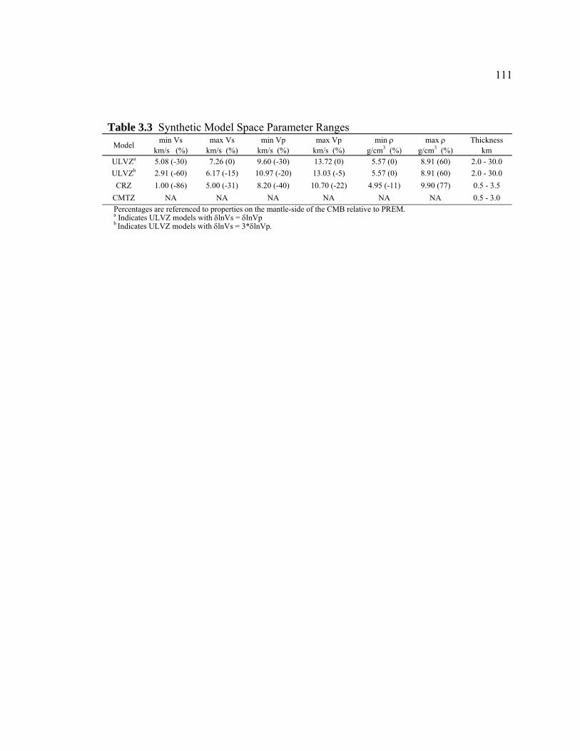
111

Table 3.3 Synthetic Model Space Parameter Ranges Model min Vs

km/s (%) max Vs

km/s (%) min Vp

km/s (%) max Vp

km/s (%) min ρ

g/cm3 (%) max ρ

g/cm3 (%) Thickness

km ULVZa 5.08 (-30) 7.26 (0) 9.60 (-30) 13.72 (0) 5.57 (0) 8.91 (60) 2.0 - 30.0 ULVZb 2.91 (-60) 6.17 (-15) 10.97 (-20) 13.03 (-5) 5.57 (0) 8.91 (60) 2.0 - 30.0

CRZ 1.00 (-86) 5.00 (-31) 8.20 (-40) 10.70 (-22) 4.95 (-11) 9.90 (77) 0.5 - 3.5 CMTZ NA NA NA NA NA NA 0.5 - 3.0

Percentages are referenced to properties on the mantle-side of the CMB relative to PREM. a Indicates ULVZ models with δlnVs = δlnVp b Indicates ULVZ models with δlnVs = 3*δlnVp.

112

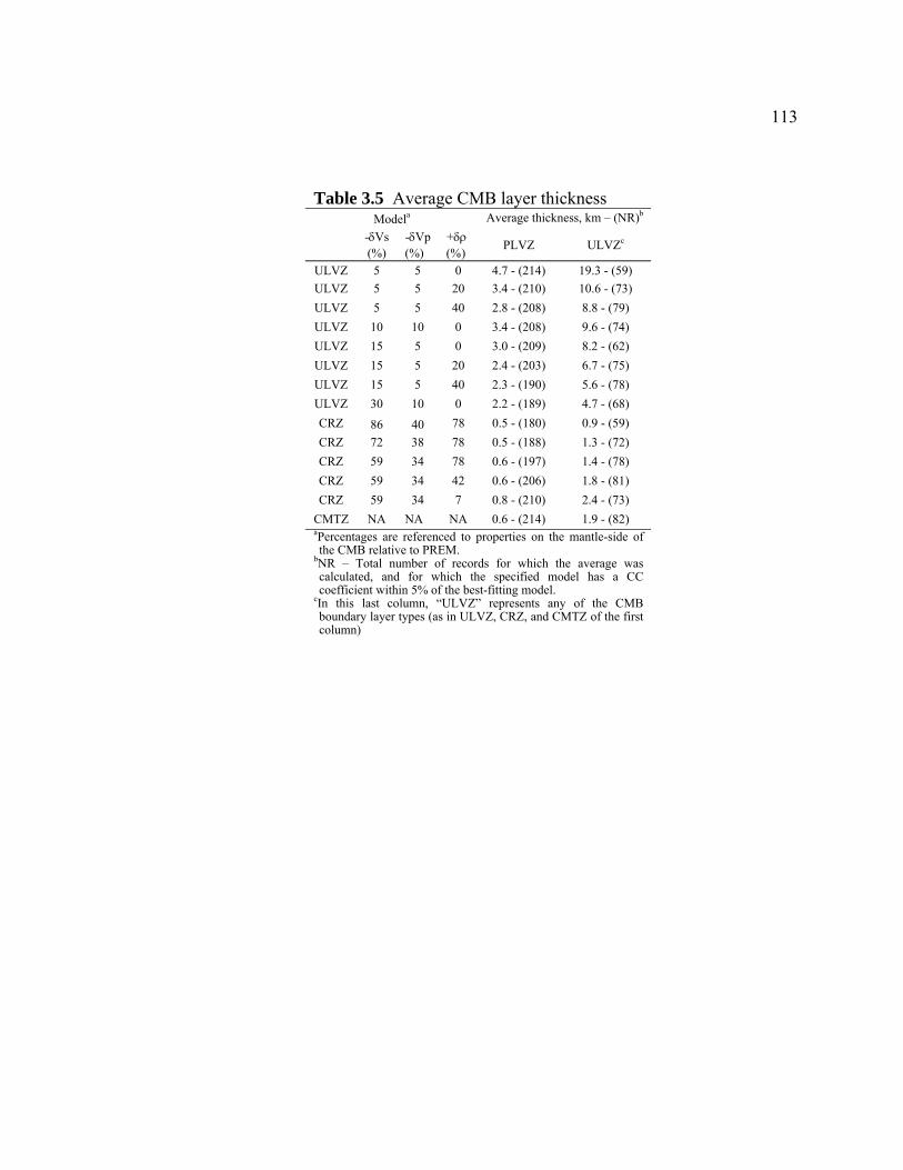
113

Table 3.5 Average CMB layer thickness Modela Average thickness, km – (NR)b

-δVs (%)

-δVp (%)

+δρ (%) PLVZ ULVZc

ULVZ 5 5 0 4.7 - (214) 19.3 - (59) ULVZ 5 5 20 3.4 - (210) 10.6 - (73) ULVZ 5 5 40 2.8 - (208) 8.8 - (79) ULVZ 10 10 0 3.4 - (208) 9.6 - (74) ULVZ 15 5 0 3.0 - (209) 8.2 - (62) ULVZ 15 5 20 2.4 - (203) 6.7 - (75) ULVZ 15 5 40 2.3 - (190) 5.6 - (78) ULVZ 30 10 0 2.2 - (189) 4.7 - (68) CRZ 86 40 78 0.5 - (180) 0.9 - (59) CRZ 72 38 78 0.5 - (188) 1.3 - (72) CRZ 59 34 78 0.6 - (197) 1.4 - (78) CRZ 59 34 42 0.6 - (206) 1.8 - (81) CRZ 59 34 7 0.8 - (210) 2.4 - (73)

CMTZ NA NA NA 0.6 - (214) 1.9 - (82) aPercentages are referenced to properties on the mantle-side of the CMB relative to PREM.

bNR – Total number of records for which the average was calculated, and for which the specified model has a CC coefficient within 5% of the best-fitting model.

cIn this last column, “ULVZ” represents any of the CMB boundary layer types (as in ULVZ, CRZ, and CMTZ of the first column)

114

FIGURES

Figure 3.1 Past study results. Panels a) and b) display details of previous studies in the

Southwest Pacific and Central American regions of the CMB respectively. The light- red

and blue shaded regions correspond to areas where ULVZ have and have not been

previously detected (Garnero et al. 1998). Red boxes, lines, and circles correspond to

locations where anomalous boundary layer structure has been inferred from previous

studies as outlined in Table 3.1 (numbers correspond to those of Table 3.1. Blue boxes,

crosses, and outlined regions correspond to locations where anomalous boundary layer

structure has previously been searched for but not observed. Black triangles correspond

to locations where anomalous boundary layer structure may exist, yet data is

inconclusive.

115

Figure 3.2 Panels a-d show the phases used in this study at four epicentral distances.

The top row of each panel shows ray paths for SKS, SPdKS (both SPdKS and SKPdS),

and SKiKS. The center row of each panel zooms in on the ray path of SKS and SPdKS for

each distance. Shown is the lateral distance along the CMB of the Pdiff portion of SPdKS

and the amount of lateral separation between SKS and SPdKS (calculated for the PREM

model), with the vertical scale exaggerated. The bottom panel shows PREM synthetic

seismograms highlighting the arrivals at each distance.

116

Figure 3.3 Distance profiles for four events. The radial component of displacement is

shown. All records are normalized and centered on the SKS peak. The predicted SPdKS

arrival for PREM is a dashed gray line and for a ULVZ model is a solid black line.

(ULVZ model: δVP = -5%, δVS = -15%, δρ = +10%, thickness = 10 km). The dotted

gray line shows the PREM prediction for the phase SKiKS. The recording station is

shown to the right of each trace. STn in panel c) corresponds to 26 stations from the

INDEPTH III PASSCAL experiment.

117

Figure 3.4 The radial component of displacement of four recording stations is shown.

All records are normalized and centered on the SKS peak. Each record is shifted in

distance to accommodate varying source depth. The predicted arrival for SPdKS is

shown for PREM (dashed gray line) and for a ULVZ model (solid black line; ULVZ

model: δVP = -5%, δVS = -15%, δρ = +10%, thickness = 10 km). Also shown (dashed

lines) are representative synthetic seismograms for this ULVZ model. Stations shown are

a) Cathedral Caves, Missouri, USA; b) Urumqi, Xinjiang, China; c) Harvard,

Massachusetts, USA; and d) Frobisher Bay, Canada.

118

Figure 3.5 Panels a, b, and c show the velocity and density profiles with depth for

ULVZ, CRZ, and CMTZ models respectively. In panels a) and b), h represents the

thickness over which mantle or core properties are modified for ULVZ or CRZ models.

In panel c, h represents the thickness over which the transition between mantle and core

properties is modeled. Relevant parameters (compared to PREM on the mantle-side) for

models shown are: a) δVS = -30%, δVP = -10%, δρ = +10%, h = 20 km; b) δVS = -72%,

δVP = -38%, δρ = +60%, h= 3 km; and c) h = 3 km.

119

120

Figure 3.6 Empirical source modeling. Panel a) displays 24 records windowed,

centered, and normalized on the SKS peak for the April 14, 1998 Fiji Islands event (#37

Table 2). The traces are all records accepted for stacking with a cross-correlation

coefficient of at least 0.85, in the distance range of 92º - 98º. In panel b), the individual

traces are overlain, with the dashed gray line indicating the resulting stack. Panel c)

displays the method of determining the empirical source, by 1) taking the synthetic

seismogram centered on SKS at 95º epicentral distance and, 2) convolving the synthetic

with a triangle or truncated triangle function (in this case, a triangle function with width

0.1 sec to the left of zero and 2.6 sec to the right of zero) that best fits the stacked data

(dashed gray line) shown in 3.

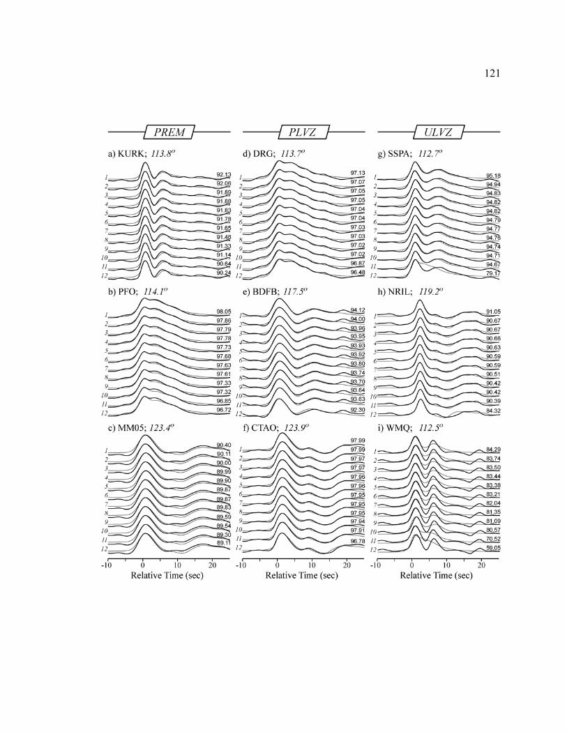
121

122

Figure 3.7 Cross-correlation of records with model synthetics. Panels a,b,c show

records classified as PREM; panels d,e,f show example records classified as PLVZ;

panels g,h show records classified as ULVZ; and panel i is an example of a record

classified as ELVZ. The dark line is data, repeated through each panel compared to the

light colored line of the synthetics. Epicentral distances and station names for each

record section is shown above the traces. Just above each data/model overlay on the right

is the CCC of the record compared to the model synthetic. Model details are contained in

Table 4 (numbers to the left of each trace correspond with Table 3.4) Events used to

make this figure are for those listed in Table 3.2 for the following dates. KURK: Dec.

18, 2000; PFO: Dec. 25, 1995; MMO5: Aug 14, 1995; DGR: Dec. 25, 1995; BDFB:

April 13, 1999; CTAO: May 10, 1994; SSPA: May 16, 1998; NRIL: March 21, 1997;

WMQ: Aug 15, 2000.

123

Figure 3.8 Panel a) shows sample PREM synthetic seismograms centered and

normalized on SKS for a 400 km deep event. Black lines show predicted arrivals for

SPdKS and SKiKS. SKiKS is observed to interfere with SPdKS waveforms in the dark

shaded region. Panel b) shows 26 records from varying events centered on SKS and

shifted to a common source depth of 400 km.

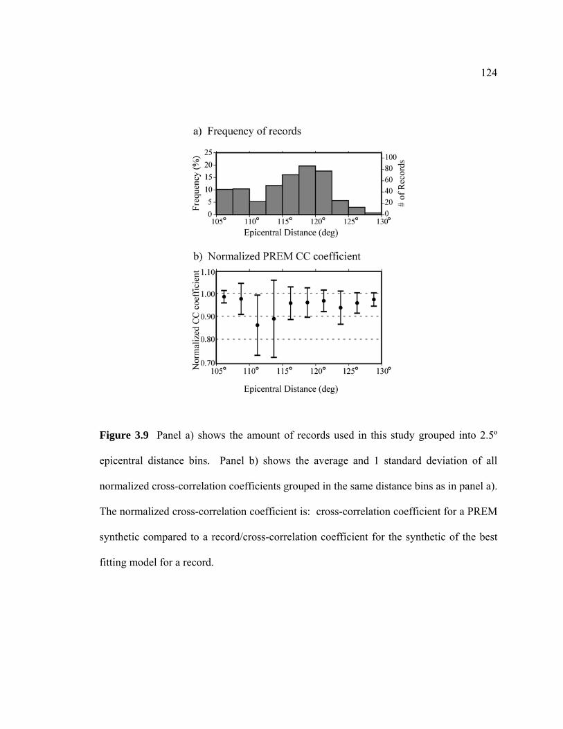
124

Figure 3.9 Panel a) shows the amount of records used in this study grouped into 2.5º

epicentral distance bins. Panel b) shows the average and 1 standard deviation of all

normalized cross-correlation coefficients grouped in the same distance bins as in panel a).

The normalized cross-correlation coefficient is: cross-correlation coefficient for a PREM

synthetic compared to a record/cross-correlation coefficient for the synthetic of the best

fitting model for a record.

125

Figure 3.10 Shown in panels a) and b) are regional maps centered in the Southwest

Pacific and Central American regions respectively. Lines drawn represent the Pdiff

segments of SPdKS on the CMB. Dark blue lines represent paths for which the

waveforms behaved as PREM. Light blue lines represent paths that are characterized as

PLVZ. Red lines are used for waveforms that are characterized as ULVZ and black lines

represent ELVZ waveforms. Stars indicate event locations and triangles represent station

locations. The distance scale beneath each panel is the distance at the equator on the

CMB.

126

127

Figure 3.11 a) Total data coverage. Green circles are stations and blue triangles are

events. Dotted lines show great circle paths between events and stations, and solid red

and light-blue lines show the Pdiff portion of SPdKS and SKPdS on the CMB respectively.

Panel b) shows the earth divided into 5° × 5° cells colored by the number of Pdiff

segments on the CMB that pass through each grid cell. Panel c) shows the earth divided

into the same grid colored by ULVZ likelihood, where a value of 1.0 signifies that all Pdiff

segments on the CMB passing through the cell had waveforms that behaved as ULVZ,

and a value of 0.0 indicates that all Pdiff segments passing through the cell had waveforms

behaving as PREM. The result is shown for the most characteristic data between 110°

and 120°. Shown in italics below the projection is the total percentage of CMB surface

area of grid cells with Pdiff segments passing through them. d-f) The average thickness is

shown for ULVZ, CRZ and CMTZ models averaged in the same grid spacing. ULVZ

model properties in panel d) are δVS = -15%, δVP = -5%, δρ = +5%. CRZ model

properties in panel e) are δVS = -59%, δVP = -34%, δρ = +42%. Model thickness is only

averaged for records where the model is within 5% of the best fitting model. For

comparison of thickness with other ULVZ models, scaling may be applied as suggested

in Table 3.5.

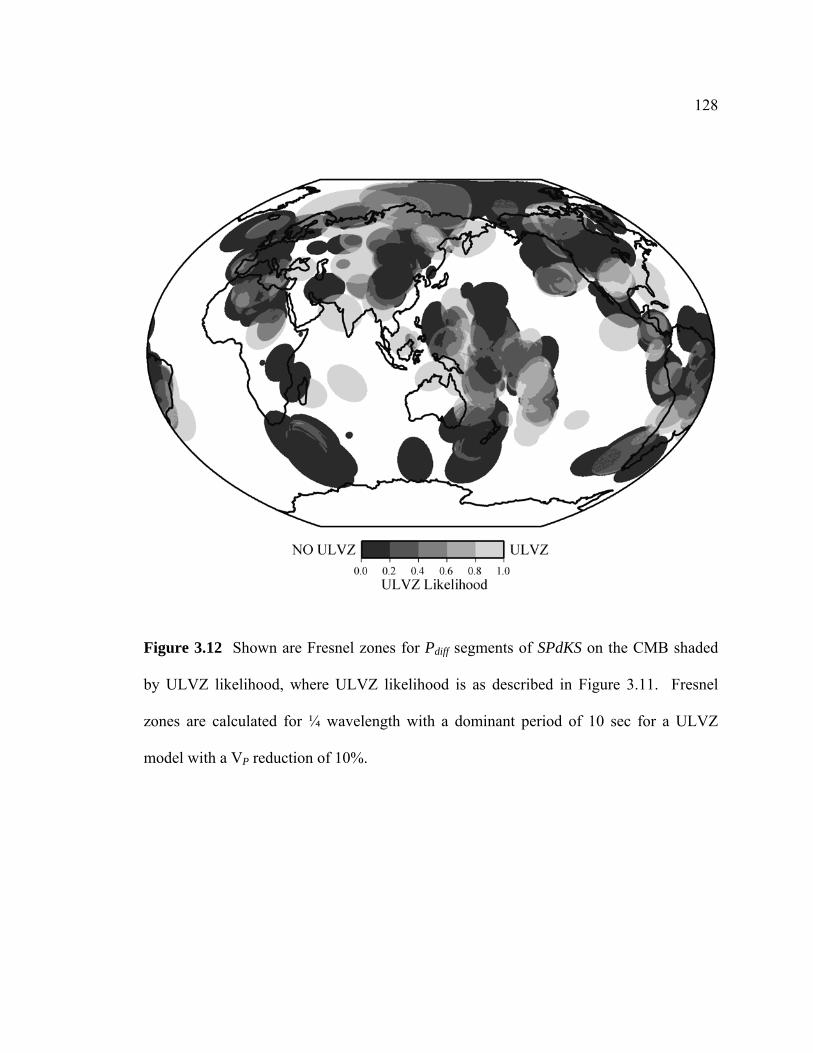
128

Figure 3.12 Shown are Fresnel zones for Pdiff segments of SPdKS on the CMB shaded

by ULVZ likelihood, where ULVZ likelihood is as described in Figure 3.11. Fresnel

zones are calculated for ¼ wavelength with a dominant period of 10 sec for a ULVZ

model with a VP reduction of 10%.

129

Figure 3.13 Shown is the comparison between SPdKS source- and receiver-side arcs

with four S-wave and three P-wave tomography models. The comparison is carried out

for all data with source-receiver distances between 110º-120º. For each tomographic

model, the average and standard deviation of the lowest velocity encounterd along a Pdiff

segment are shown. Individual model results are grouped into categories of PREM,

PLVZ, and ULVZ waveform classifications. S-wave models are: TXBW (Grand 2002),

saw24b16 (Megnin & Romanowicz 2000), s20rts (Ritsema & van Heijst 2000), and

s362c1 (Gu et al. 2001). P-wave models are: kh2000pc (Kárason & van der Hilst 2001),

Zhao (Zhao 2001), bdp98 (Boschi & Dziewonski 1999).

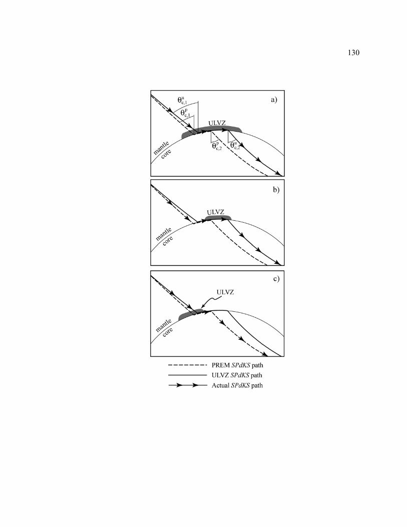
130

131

Figure 3.14 The source-side SPdKS ray path geometry is shown for three different

possibilities of ULVZ location. The dashed line indicates the path SPdKS would take if

the mantle were purely PREM, and the solid line indicates the path SPdKS would take if

there existed a 30 km thick ULVZ (δVS = -15%, δVP = -5%, δρ = +0%) at the base of the

mantle. Arrows outline the actual path SPdKS takes. In panel a), the ray path encounters

the ULVZ and becomes critical at an angle of . The Puc 1,θ diff path continues through the

ULVZ and exits at the same critical angle . If the ULVZ did not exist, the ray path

would follow the PREM prediction and become critical at angle with the P

uc 2,θ

pc 1,θ diff path

also exiting at that angle ( ). In panel b), no ULVZ exists at the inception point of Ppc 2,θ diff

and becomes critical at angle . However, Ppc 1,θ diff encounters the ULVZ along its path

and thus exits at the critical angle for the ULVZ model . In panel c) the situation is

reversed from panel b). The geometry of the ray paths was calculated for a source-

receiver distance of 115° and a source depth of 500 km.

uc 2,θ

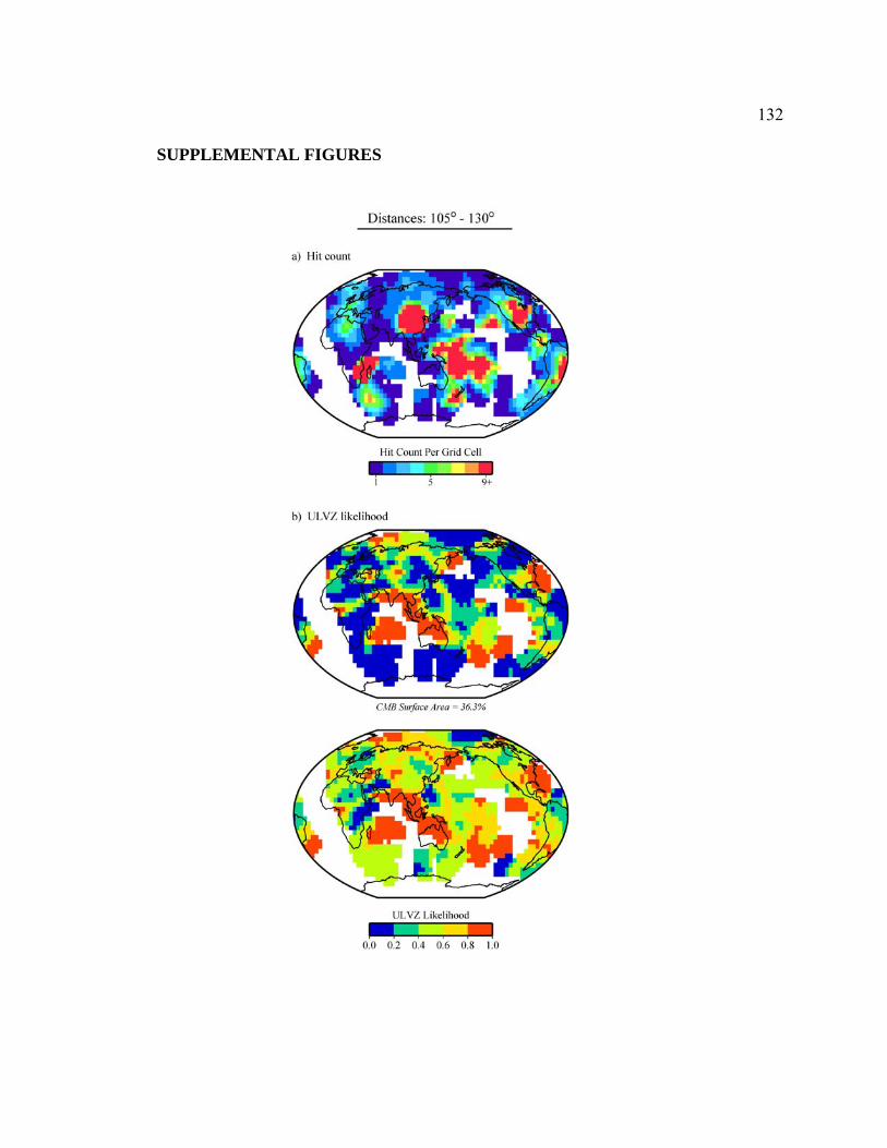
132

SUPPLEMENTAL FIGURES

133

Supplement 3A Panel a shows the earth divided into 5° x 5° cells colored by the number

of Pdiff segments on the CMB that pass through each grid cell. The result is shown for all

data used in this study in the distance range 105° to 130°. Panel b shows the earth

divided into 5° x 5° cells colored by ULVZ likelihood, where a value of 1.0 signifies that

all Pdiff segments on the CMB passing through the cell had waveforms that behaved as

ULVZ, and a value of 0.0 indicates that all Pdiff segments passing through the cell had

waveforms behaving as PREM. The result is shown when all data is included. For the

top figure of panel b, ULVZ likelihood calculations were made with PREM- and PLVZ-

waveforms given a value=0, and ULVZ- and ELVZ-waveforms given a value=1. For the

bottom plot of panel b, PREM-waveforms were given a value=0, PLVZ-waveforms were

given a value=0.5, and ULVZ- and ELVZ-waveforms were given a value=1. This figure

differs from Figure 3.11, in that PLVZ-waveforms were there given a value=0, and this

figure also shows the result when considering our entire data set. The bottom figure of

panel b shows the pervasiveness of ULVZ structure that may exist if PLVZ-waveforms

actually represent thin ULVZ structure.

CHAPTER 4

COMPUTING HIGH FREQUENCY GLOBAL SYNTHETIC SEISMOGRAMS

USING AN AXI-SYMMETRIC FINITE DIFFERENCE APPROACH

Michael S. Thorne1

1Dept. of Geological Sciences, Arizona State University, Tempe, AZ 85287, USA 4.1 Introduction

Resolving Earth’s seismic structure is crucial in order to understand Earth’s

dynamics, composition, and evolution. Waveform modeling is an exceptional tool for

modeling Earth’s seismic structure, by comparing real seismograms with synthetic

seismograms computed for realistic Earth models. Numerous techniques for computing

synthetic seismograms by solving the wave equation for seismic wave propagation have

been developed over the last 40 years. Many of these techniques have been based on

analytical solutions and/or the assumption of spherical symmetry (e.g., Helmberger 1968;

Fuchs & Müller 1971; Woodhouse & Dziewonski 1984). Recently, advances in

distributed memory, or cluster, computing have made numerical techniques for solving

the wave equation viable, thus allowing computation of synthetic seismograms for a wide

range of heterogeneous Earth models at frequencies relevant to broadband and short

period waveform modeling.

Numerical techniques are important because synthetic seismograms can be

computed for models of a highly heterogeneous nature where analytical solutions may be

difficult to obtain. Finite difference (FD) techniques are the most common numerical

techniques in practice; however other numerical techniques are also used frequently. The

most common numerical techniques currently in use are:

135

1) pseudo-spectral technique (e.g., Fornberg 1987; Furumura et al. 1998; Cormier

2000),

2) spectral element technique (e.g., Komatitsch & Tromp, 2002),

3) finite element technique (e.g., Smith 1975), and

4) finite volume technique (e.g., Dormy & Tarantola 1995).

Each technique has strengths and weaknesses and may be suitable for different styles of

problems (see Carcione et al. 2002 for a review).

Finite difference techniques have been used to calculate seismic wave propagation

for nearly 40 years since the first applications by Alterman & Karal (1968) and Alterman

et al. (1970). Madariaga (1976) was the first to use a velocity-stress FD formulation, the

most common formulation currently in use. The first 2-D Cartesian grid FD simulations

were carried out for SH-waves by Virieux (1984) and Vidale et al. (1985). Virieux

(1986) and Levander (1988) carried out the first 2-D Cartesian grid FD simulations for P-

SV wave propagation. The first 3-D Cartesian grid FD simulations were performed

shortly thereafter (e.g., Randall 1989). All of the aforementioned simulations were

limited to small regional dimensions, mostly due to limited computational resources. An

abundance of studies on FD methods for wave propagation have been developed over the

decades and an excellent overview is given in Moczo et al. (2004).

In this paper we apply a 3-D axi-symmetric FD approach. First we outline the

method, then show an example application of the method by simulating seismic coda

waves through models containing randomly distributed heterogeneous S-wave velocity

136

perturbations. This is the first study in which a FD technique has been employed for

whole mantle scattering.

4.2 3-D axi-symmetric finite difference wave propagation

The 3-D axi-symmetric FD method for SH-waves (SHaxi) is developed because it

is less computationally expensive than fully 3-D methods. This is because axi-symmetry

allows the calculation to be performed on a 2-D grid. Hence, we are able to obtain

frequencies relevant to broadband waveform modeling (e.g., up to 1 Hz dominant

frequencies) that are not currently feasible using 3-D methods. The axi-symmetric

approach is also attractive as the correct 3-D geometrical spreading is naturally

incorporated which fully 2-D techniques must approximate.

Axi-symmetric FD methods have been applied in the past. Igel & Weber (1995)

were the first to compute axi-symmetric wave propagation for SH-waves. The technique

was then applied to studying long period SS-precursors by Chaljub & Tarantola (1997).

Igel & Gudmundsson (1997) also used the method to study frequency dependent effects

of S and SS waves. Igel & Weber (1996) developed an axi-symmetric approach for P-SV

wave propagation. Thomas et al. (2000) developed an axi-symmetric method for

acoustic wave propagation and applied the technique to studying precursors to PKPdf.

Recently, Toyokuni et al. (2005) have also developed an axi-symmetric method for SH-

wave propagation.

The axi-symmetric FD technique for SH-waves (SHaxi) first developed by Igel &

Weber (1995) has recently been expanded to operate on distributed memory computers

137

and to include higher order FD operators (Jahnke et al. 2005). These advances have

given the SHaxi technique the ability to compute synthetic seismograms for higher

frequencies (up to 1 Hz) than have previously been possible. In this Section we present

the technique behind SHaxi. Verification of the SHaxi method is presented in Jahnke et

al. (2005).

4.2.1 The axi-symmetric wave equation

The displacement-stress formulation of the wave equation in spherical coordinates

can be written as follows:

( ) rrrrrrrrr f

rrrrtu

++−−+∂

∂+

∂∂

+∂

∂=

∂∂

θσσσσϕ

σθθ

σσρ θϕϕθθ

ϕθ cot21sin11

2

2

(4-1)

( )( θθϕϕθθθϕθθθθ σθσσ

ϕ)σ

θθσσ

ρ frrrrt

ur

r ++−+∂

∂+

∂∂

+∂

∂=

∂∂

3cot1sin11

2

2

(4-2)

( ϕθϕϕϕϕθϕϕϕ θσσ

ϕσ

θθσσ

ρ frrrrt

ur

r +++∂

∂+

∂

∂+

∂

∂=

∂

∂cot231

sin11

2

2

) , (4-3)

where ρ is density, u is displacement, σ is stress and f is a body force. The coordinate

system adopted is displayed in Figure 4.1.

For the case of SH-wave propagation we are only concerned with the

displacement in the φ-direction therefore only eq. (4-3) is applicable. Because of axi-

symmetry the ∂/∂φ terms go to zero and eq. (4-3) reduces to:

( ϕθϕϕθϕϕϕ θσσ

θσσ

ρ frrrt

ur

r +++∂

∂+

∂

∂=

∂

∂cot2311

2

2

) . (4-4)

138

Vireux (1984) showed that FD simulations can attain greater accuracy using a

staggered grid (see Section 4.3.1) and the velocity-stress formulation. The SHaxi method

adopts this staggered grid and velocity-stress formulation, thus we are left with the

following axi-symmetric wave equation to solve:

( ϕθϕϕθϕϕϕ θσσ

θ)σσ

ρ frrrt

vr

r +++∂

∂+

∂

∂=

∂

∂cot2311 , (4-5)

where v, is the velocity.

4.2.2 The strain tensor

Solving the wave equation as presented in eq. (4-5) consists of a two-step

procedure. In the first step we update the strain tensor from the velocity field and then

calculate the stress tensor from the strain tensor. Once the stress tensor is updated we can

update the velocity field in the second step from equation (4-5). Equation 1.56 of Ben-

Menahem & Singh (1981) gives the expressions for the strain tensor in spherical

coordinates:

rur

rr ∂∂

=ε (4-6)

⎟⎠⎞

⎜⎝⎛ +

∂∂

= ruu

r θε θ

θθ1 (4-7)

⎟⎟⎠

⎞⎜⎜⎝

⎛++

∂

∂= θ

ϕθε θ

ϕϕϕ cot

sin11 uu

ur r (4-8)

⎟⎟⎠

⎞⎜⎜⎝

⎛∂∂

+−∂

∂==

ϕθθ

θεε θ

ϕϕ

ϕθθϕu

uu

r sin1cot

21 (4-9)

139

⎟⎟⎠

⎞⎜⎜⎝

⎛−

∂

∂+

∂∂

==r

ur

uur

rrr

ϕϕϕϕ ϕθ

εεsin1

21 (4-10)

⎟⎠⎞

⎜⎝⎛

∂∂

+−∂

∂==

θεε θθ

θθr

rru

rru

ru 1

21 , (4-11)

where ε is the strain. For SHaxi we can see from inspection with eq. (4-5) that only σθφ

and σrφ need to be calculated. Hence we only need to calculate the strain components εθφ

and εrφ from eqs. (4-9) and (4-10). In the axi-symmetric velocity-stress formulation these

two equations reduce to:

⎟⎟⎠

⎞⎜⎜⎝

⎛−

∂

∂=

∂

∂θ

θε

ϕϕθϕ cot

21 v

vrt

(4-12)

⎟⎟⎠

⎞⎜⎜⎝

⎛−

∂

∂=

∂

∂

rv

rv

tr ϕϕϕε

21 . (4-13)

4.2.3 The stress tensor

Once the strain tensor is determined, the stress calculation is straightforward. From

Hooke’s Law:

rrrrrr M++∆= µελσ 2 (4-14)

θθθθϕϕ µελσ M++∆= 2 (4-15)

ϕϕϕϕϕϕ µελσ M++∆= 2 (4-16)

θθθ µεσ rrr M+= 2 (4-17)

θϕθϕθϕ µεσ M+= 2 (4-18)

ϕϕϕ µεσ rrr M+= 2 , (4-19)

140

where λ and µ are the Lamé parameters (µ is the shear modulus), ∆ is the dilatation or

trace of the strain tensor, and M is the seismic moment. For the SH-case, only eqs. (4-18)

and (4-19) need to be calculated. In general seismic sources can be added to the

simulation by addition of appropriately scaled moment tensor elements (Mij) in this step

(e.g., Coutant 1995; Graves 1996). However, direct application of moment tensor

elements may be challenging in SHaxi due to the axi-symmetric boundary condition and

we do not concern ourselves with moment tensor addition. A description of how the

source is implemented is given in Section 4.3.6.

4.3 Finite difference implementation

4.3.1 Finite difference grid

SHaxi solves the wave equation on a 2-D grid as shown in Figure 4.2. The grid is

bound between radii of 3480 to 6371 km, and theta values between 0° and 180°. A few

grid points exist outside of these bounds in order to compute the boundary conditions (see

Section 4.3.3). Virieux (1986) introduced a staggered grid system for FD simulations of

the wave equation, which improved numerical accuracy over other grid systems. As a

result most current FD methods for solving the wave equation incorporate the staggered

grid formulation (e.g., Coutant et al. 1995; Igel & Weber 1995; 1996, Graves 1996;

Chaljub & Tarantola, 1997; Igel et al. 2001; Takenaka et al. 2003). Detail of the

staggered FD grid used by SHaxi is shown in Figure 4.3. The correspondence between

grids shown in Figures 4.2 and 4.3 can be seen in that each grid point crossing shown in

Figure 4.2 corresponds to a velocity (vφ) grid point in Figure 4.3.

141

It can be shown that the staggered grid produces more accurate results by

considering the error in FD approximations (Igel, 2002). Using a staggered grid system,

the spatial derivatives of discrete fields such as velocity or stress, are calculated halfway

between the defined grid points. The SHaxi method utilizes a centered difference FD

scheme. For example, using a two-point finite difference operator we may approximate

the spatial derivative as follows:

dxdxxfdxxf

xf

2)()( −−+

≈∂∂ . (4-20)

If we expand equation 4-2-22 using a Taylor series expansion, recalling that the Taylor

series expansion is given by:

...)(''''!4

)('''!3

)(''!2

)(')()(432

±+±+±=± xfdxxfdxxfdxxdxfxfdxxf . (4-21)

Then we may rewrite 4-2-22 as:

)()('...)('''!3

)('1)2/()2/( 23

dxOxfxfdxxdxfdxdx

dxxfdxxf+=⎥

⎦

⎤⎢⎣

⎡++=

−−+ . (4-22)

The error of the first derivative is of the order dx2, or is proportional to the size of the FD

grid step over which the derivative is approximated. Reducing the size of the grid step by

half reduces the error of the approximation by a factor of four.

4.3.2 Boundary Conditions

There are two cases of boundary conditions in SHaxi. The first case occurs at the

symmetry axes (located at θ=0° and θ=180°; see Figure 4.2). At the symmetry axes a

reflecting boundary condition is defined as:

142

,

0

2/2/

2/2/

,0

θπθθϕθπθθϕ

θθθϕθθθϕ

θπθϕθπθϕ

θθϕθθϕ

πθθϕ

σσ

σσ

ndnd

ndnd

ndnd

ndnd

vv

vv

v

−=+=

+=−=

−=+=

+=−=

==

=

=

=

=

=

(4-23)

where n is an integral number of grid points from the symmetry axis. The second case

occurs at the free surface. Here we use the zero-stress condition where σrφ must go to zero

(e.g., Levander 1988; Graves 1996). The zero-stress condition can be met by giving the

vφ and σrφ values above the free surface the opposite of the values below the free surface.

Because the CMB is a perfect reflector for SH-waves, the zero-stress condition is also

used there. The zero-stress boundary condition is defined as:

,2/2/

2/2/

ndrRrrndrRrr

ndrRrrndrRrr

ndrRrndrRr

ndrRrndrRr

CMBCMB

EE

CMBCMB

EE

vv

vv

+=−=

−=+=

+=−=

−=+=

−=

−=

−=

−=

ϕϕ

ϕϕ

ϕϕ

ϕϕ

σσ

σσ (4-24)

where n is an integer number of grid points from the free surface or CMB.

4.3.3 Source implementation

Because of axi-symmetry, in particular due to the cot θ term in eq. (4-5), the

source cannot be placed directly on the symmetry axis but rather must be placed at a grid

point adjacent to the symmetry axis. In SHaxi we apply a body force to one of the

velocity field grid points. With the reflecting boundary condition, this is seen as a

reflection on the velocity grid point directly opposite the source insertion grid point

143

across the symmetry axis. This source implementation does not produce a seismic source

similar to a double-couple, but instead approximates a single-couple. By axi-symmetry

the source is effectively rotated in the φ-direction and is thus a ring of single-couples.

The source radiation pattern for this type of source is derived in Jahnke et al. (2005). The

most notable aspect of this type of source is its strong dependence on take-off angle,

where the amplitude of the source radiation is proportional to the sine of the take off

angle. This is demonstrated in Figure 4.4.

Implementing a source-time function in SHaxi can be accommodated in two

ways. The first way is to provide a step-impulse function applied as a body force (f in eq.

4-5). As displacement is proportional to the first derivative of the moment function,

resulting displacement seismograms are delta functions. This technique propagates

energy at all frequencies and after completion of the computation, the synthetic

seismograms must be filtered to remove higher frequency content that is invalid for the

FD grid. Any source time function can then be implemented by convolving a source-

time function with the delta function output, so long as the frequency content of the

source-time function is long enough period to be valid. This is our preferred method for

implementing sources when synthetic seismograms are the desired output. Alternatively,

a smooth function with finite frequency content can be applied directly as a body force.

This method is preferred for producing snapshots of wave propagation. The source-time

function used in this case is:

( ) ( ) ( )tinnntin ptprrrptprtS )2(sin2sin)( ++−= [ ] tpt <

( ) ( ) ( )innnin prrrprtS )2(sin)2(sin)( ++−= , [ ] tpt ≥(4-25)

144

where pi = 4*atan(1), pt is the dominant period, and rn is the number of extrema. To

reproduce a smoothly varying step function, appropriate to produce a Gaussian shaped

displacement pulse we choose rn = 0.001.

4.3.4 Parallelization

The SHaxi method is parallelized to operate on distributed memory computer

systems. The Message Passing Interface (MPI) is used to control communication

between separate processors. The parallelization is implemented as shown in Figure 4.2.

The SHaxi grid is subdivided laterally (in the θ-direction) into a user-defined number of

separate ranks. Each processor is responsible for updating the wavefield in each rank.

Overlapping grid points (in number corresponding to the FD operator length divided by

two) are used in the SHaxi grid (located at the maximum θ value for each rank) to

accommodate this parallelization. Communication at each time step need only update

overlapping grid points.

The advantage of the parallelization is that synthetic seismograms can be

computed much more rapidly than on single processor machines allowing computation of

relatively high frequency synthetics on modest Linux clusters. Table 4.1 lists some

sample grid dimensions, attainable dominant periods, computational memory

requirements, and performance for parallel jobs. The values given in Table 4.1 are for a

Linux cluster (located at Arizona State University) with Intel® Xeon™ 2.40 GHz CPU’s.

Values given are for a source-code compiled using the Intel® Fortran Compiler for Linux

(ifort v. 9.0) with Single SIMD Extensions (SSE) enabled. From Table 4.1 it can be seen

145

that the run time is roughly proportional to the number of grid points × the number of

timesteps. The slight decrease in performance for larger models is likely due to the

limited cache size. The performance listed in Table 4.1 corresponds to simulation times

of 2700 sec. It should be noted however, that total run time is not linearly related to

simulation time. This is because computation time at each time step increases with

increasing simulation time as the wavefield spreads throughout the grid. Many

simulations do not need to be computed to 2700 sec (e.g., 1700 sec is appropriate for the

models discussed in Chapter 5) and much quicker performance is attained. SHaxi also

has the ability to perform the calculation on a limited domain size in the θ-direction.

That is, an absorbing boundary can be placed at an arbitrary grid location. For example,

placing an absorbing boundary at 90° would reduce the total grid size by half and

dramatically reduce computation time. The total run times listed in Table 4.1 are for

longer simulations and represent the higher end of SHaxi’s computational demands.

4.3.5 3-D Axi-symmetric model structure

Although SHaxi implements models on a 2-D grid, the formulation of the wave

equation (eqs. 4-5, 4-12, 4-13) is for 3-D axi-symmetry or model invariance in the φ-

direction. This means that models are constructed along the great-circle arc plane

between source and receiver with no model variation off of the great-circle arc plane. In

essence, the model placed on the 2-D grid is rotated about the φ-direction. To understand

this, consider placing S-wave velocity anomalies on SHaxi’s grid as shown in Figure 4.5.

Rotating this model in the φ-direction produces the model shown in Figure 4.6. The

146

result of this model construction is that seismic amplitudes may be over- or under-

predicted from amplitudes expected from fully 3-D models. For example, if the high-

velocity anomaly (blue filled area) of Figure 4.5 were actually spherically shaped (and

not ring-shaped as in Figure 4.6), the seismic wavefield would be slowed down in its path

around the off great-circle arc plane in the presence of this anomaly. Therefore, the

amplitudes of the latter portion of the arrival would be diminished. Despite this

introduction of ring-like anomalies, the absolute arrival time information is not corrupted.

4.3.6 PREM Synthetic Seismograms

As an example of using the SHaxi method we show synthetic seismograms

computed for the PREM model (Dziewonski & Anderson 1981). One advantage of the

SHaxi method is the ease in which snapshots of wave propagation can be produced.

Snapshots at three time steps are shown in Figure 4.7. Five-second dominant period

synthetic seismograms for this run are shown in Figure 4.8. Here we show a small

window of the wavefield between 70º and 85º encompassing the S and SS arrivals. A

clear advantage of numerical techniques can be seen in Figure 4.8, in that the entire

wavefield is calculated. This can be seen by all of the minor arrivals apparent in between

the dominant arrivals that are labeled, corresponding to crustal and mid-crustal

reverberations, reflections from first-order discontinuities, etc. An exhaustive list of

arrivals apparent in Figure 4.8 is beyond the scope of this chapter (For a list of some of

the arrivals apparent in a narrow time window of Figure 4.8 see Supplement 5A in

Chapter 5).

147

4.4 Application: Whole mantle scattering

4.4.1 Seismic scattering in the mantle

Propagating seismic waves lose energy due to geometrical spreading, intrinsic

attenuation and scattering attenuation. The scattering, or interaction with small spatial

variations of material properties, of seismic waves affects all seismic observables

including amplitudes and travel-times and also gives rise to seismic coda waves. Seismic

coda are wave trains that trail dominant seismic arrivals. For example, high frequency P-

waves exhibit energy decaying over hundreds of seconds after the direct arrival.

Much of seismic analysis is done where the length scales of velocity perturbations

are much larger than the wavelength of the seismic phase of interest. In this case, ray

theoretical approaches such as seismic tomography have dominated seismic analyses and

have provided large-scale length views of Earth’s seismic properties (e.g., Ritsema & van

Heijst 2000; Grand 2002). Aki (1969) first demonstrated that seismic coda waves might

be produced by random heterogeneity with length scales of velocity perturbations on the

order of the wavelength of the seismic phase. Analysis of seismic coda waves has thus

provided a method to quantify small-scale seismic properties that cannot be determined

through travel-time analysis or ray theoretical approaches.

Many techniques have been developed to study the properties of seismic

scattering (see Sato & Fehler, 1998 for a discussion on available techniques). Recently,

advances in computational speed have allowed numerical methods such as FD techniques

to be utilized in analyzing seismic scattering (e.g., Frankel & Clayton 1984, 1986;

Frankel 1989; Wagner 1996). The majority of FD studies have thus far focused on S-

148

wave scattering in regional settings with source-receiver distances of just a few hundred

kilometers. This has greatly improved our understanding of scattering in the lithosphere

where strong scattering is apparent with S-wave velocity perturbations on the order of 5

km in length and 5% RMS velocity fluctuations (e.g., Saito et al. 2003).

Recently, small-scale scattering has been observed near the core-mantle boundary

(CMB). Cleary & Haddon (1972) first recognized that precursors to the phase PKP

might be due to small-scale heterogeneity near the CMB. Hedlin et al. (1997) also

modeled PKP precursors with a global data set. They concluded that the precursors are

best explained by small-scale heterogeneity throughout the mantle instead of just near the

CMB. Hedlin et al.’s (1997) finding suggests scatterers exist throughout the mantle with

correlation length scales of roughly 8 km and 1% RMS velocity perturbation. Margerin

& Nolet (2003) also modeled PKP precursors corroborating the Hedlin et al. (1997) study

that whole mantle scattering best explains the precursors. Although Margerin & Nolet

suggest a slightly smaller RMS perturbations of 0.5% on length scales from 4 to 24 km.

Recently, Lee et al. (2003) examined scattering from S and ScS waves beneath central

Asia finding that scattering from ScS waves may dominate over the scattering from S

waves at dominant periods greater than 10 sec and that as much as 80% of the total

attenuation of the lower mantle may be due to scattering attenuation. Because Lee et al.

(2003) utilized radiative transfer theory to model scattering coefficient; it is not possible

to directly translate the scattering coefficients determined in their study to correlation

length scales or RMS perturbations (personal communication, Haruo Sato, 2005) for

comparison with the studies of Hedlin et al. (1997) or Margerin & Nolet (2003).

149

Nevertheless, their conclusion is important in that whole mantle scattering is necessary to

model their data.

Baig & Dahlen (2004) sought to constrain the maximum allowable RMS

heterogeneity in the mantle as a function of scale length. Their study also suggests as

much as 3% RMS S-wave velocity perturbations are possible for the entire mantle for

scale lengths less than roughly 50 km. Baig & Dahlen (2004) also suggest that in the

upper 940 km of the mantle scattering may be twice as strong as in the lower mantle.

The suggestion of stronger upper mantle scattering is also supported by Shearer & Earle

(2004). Shearer & Earle (2004) find that in the lower mantle 8 km scale length

heterogeneity with 0.5% RMS perturbations can explain P and PP coda for earthquakes

deeper than 200 km. They find that shallower earthquakes require stronger upper mantle

scattering with 4-km scale lengths and 3-4% RMS perturbations.

Although, a growing body of evidence suggests whole mantle scattering is

necessary to explain many disparate seismic observations, the characteristic scale lengths

and RMS perturbations are determined using analytical and semi-analytical techniques

which in many cases are based on single-point scattering approximations and do not

synthesize waveforms. As whole mantle scattering may affect all aspects of seismic

waveforms, it is thus important to synthesize global waveforms with the inclusion of

scattering effects. The first attempt at synthesizing global waveforms was by Cormier

(2000). He utilized a 2-D Cartesian pseudo-spectral technique to demonstrate that the D"

discontinuity may due to an increase in the heterogeneity spectrum. Cormier (2000)

150

suggests that as much as 3% RMS perturbations may be possible for length scales down

to roughly 6 km.

4.4.2 Construction of random velocity perturbations – Summary

Random velocity perturbations (we refer to models of random velocity perturbations

as random media hereafter) are characterized by their spatial autocorrelation function, the

Fourier transform of which equals the power spectrum of the velocity perturbations.

Construction of random media for FD simulations is implemented using a Fourier based

method (e.g., Frankel & Clayton 1986; Ikelle et al. 1993; Sato & Fehler 1998). In this

section we provide an outline of the method. The basic steps in creating random velocity

perturbations are outlined below:

1) Create a matrix of uncorrelated random numbers θ(x,y) on the interval [0, 2π].

2) Create an autocorrelation matrix auto(x,y) with the same dimensions as θ.

3) Fast Fourier Transform (FFT) θ and auto into the wavenumber domain.

4) In the wavenumber domain, multiply θ and auto, corresponding to convolution.

5) Inverse FFT the random media back to the spatial domain.

6) Window the velocity variations so as to not be outside of the range of the FD

numerical stability.

In what follows we describe the six steps outlined above in greater detail.

151

4.4.3 Construction of random velocity perturbations - Details

1) A matrix of uncorrelated random numbers (θ) is generated with a Gaussian

probability distribution with dimensions equal to the model size. The random

distributions are also scaled on the interval [0,2π] so that they do not individually need to

be Fourier transformed later. Figure 4.9 shows 2 realizations of initial random matrices.

2) The spectral characteristics of random inhomogeneities are described by

autocorrelation functions (ACF). The most popular choice of ACF’s are defined:

Gaussian: auto(x, y) = e−r 2

a 2 (4-26)

Exponential: auto(x, y) = e−r

a (4-27)

von Karman: auto(x,y) =1

2m−1Γ(m)ra

⎛ ⎝ ⎜

⎞ ⎠ ⎟

m

Kmra

⎛ ⎝ ⎜

⎞ ⎠ ⎟ , (4-28)

where r is the offset or spatial lag: r = x 2 + y 2 + z2 , and a is the autocorrelation length

(ACL). The ACFs given in eqs. (4-26) through (4-28) are shown in Fig. 4.11. These

three ACFs are most predominantly used, however many other choices also exist (e.g.,

Klimeš 2002a; 2002b).

The definition of the von Karman ACF given in eq. (4-28) is taken from Frankel &

Clayton (1986), where Km(x) is a modified Bessel function of the second kind of order m

and Γ(m) is the gamma function. Modified Bessel functions are solutions to the

following differential equation:

0)( 222

22 =+−+ ymx

xyx

xyx

∂∂

∂∂ . (4-29)

The general solution to this differential equation is:

152

y(x) = c1Im (x) + c2Km (x), (4-30)

where Im(x) and Km(x) are the modified Bessel functions of the first and second kind

respectively. Frankel and Clayton (1986) limit their discussion to Bessel functions of

order m = 0, yet the order can vary between 0.0-0.5. In the case of order m = 0.5, the von

Karman ACF is identical to the Exponential ACF. Fig. 4.10 shows Bessel functions of

the second kind.

The ACF definitions given in eqs. (4-26) through (4-28) represent isotropic ACFs

because the ACLs are the same in the three principal directions. Ikelle et al. (1993) also

define an anisotropic exponential ACF, which they refer to as an Ellipsoidal ACF. Ikelle

et al. (1993) considers 2-D media and their definition allows for ACLs in the x- and y-

principal directions to be different from each other. We generalize their definition for the

ACFs listed in eqs. (4-26) through (4-28) to allow for anisotropic ACLs in all three

dimensions for each ACF:

Gaussian: auto(x, y) = e−

x 2

alx 2+

y 2

aly 2+

z 2

alz2

⎛

⎝ ⎜

⎞

⎠ ⎟

(4-31)

Exponential: auto(x,y) = e−

x 2

alx 2 +y 2

aly 2 +z 2

alz 2

(4-32)

von Karman: auto(x,y) =1

2m−1Γ(m)x 2

alx 2 +y 2

aly 2 +z2

alz2

⎛

⎝ ⎜ ⎜

⎞

⎠ ⎟ ⎟

m

Kmx 2

alx 2 +y 2

aly 2 +z2

alz2

⎛

⎝ ⎜ ⎜

⎞

⎠ ⎟ ⎟ ,

(4-33)

where alx, aly, and alz are the ACLs in the x-, y-, and z- principal directions.

153

3) Once an autocorrelation matrix has been created the realization of random media is

accommodated in the wavenumber domain by FFT. This is because the Fourier

transform of the autocorrelation function is equal to the power spectrum of the random

media (e.g., Frankel 1989).

The primary difference between ACFs is defined by their roughness. The power

spectrum of an ACF is flat out to a corner wavenumber that is roughly proportional to the

inverse of the ACL. From the corner wavenumber the power spectrum asymptotically

decays. The roughness is a measure of how fast the rate of fall of is. In order to examine

the ACF’s roughness we must first describe the FFT of an ACF and then describe how

the random media is realized.

The Fourier Transform is typically defined in terms of a time-frequency transform.

Nevertheless, the Fourier Transform is also valid in the distance-wavenumber domain. In

the frequency domain we define the continuous time Fourier Transform as:

dtethfH ift∫∞

∞−

= π2)()( , (4-34)

where f is the frequency with units [sec-1 or Hz]. In the space-wavenumber domain we

replace ω with radial wavenumber k with units [rad/m]. As with the temporal case ω =

2πf we also have a spatial counterpart k = 2πK where K is the wavenumber [m-1]. Hence

if we are concerned with spatial variations we can write the Fourier Transform as:

drerhKH iKr∫∞

∞−

= π2)()( , (4-35)

and the inverse transform as:

154

∫∞

∞−

−= dKeKHrh iKrπ2)()( . (4-36)

Because the Fourier transform of the ACF determines the power spectrum of the

random media it is worthwhile to look at the power spectrum of the three classes of

ACFs. First we will derive the Fourier transform of the 1-D isotropic exponential ACF.

Substituting equation (4-27) into (4-35) we obtain:

dreeKH ikrar

π2)( ∫∞

∞−

−= (4-37)

dreedreeKH iKrariKra

r ππ 2

0

02)( ∫∫

∞−

∞−

+=⇒ (4-38)

iKaa

iKaaKH

ππ 2121)(

−+

+=⇒ (4-39)

⇒ H(K) =2a

1+ 4π 2K 2a2 (4-40)

Or, because k=2πK => k2=4π2K2, and we can write:

H(k) =2a

1+ k 2a2 (4-41)

Frankel & Clayton (1986) define the Fourier transform for 1-D and 2-D isotropic ACFs.

These Fourier transforms are:

1-D Isotropic ACF Fourier Transforms:

Gaussian: H(k) = (π )1

2 ae−k 2a 2

4 (4-42)

Exponential: H(k) =2a

1+ k 2a2 (4-43)

155

von Karman (Order=0): H(k) =a

1+ k 2a2( )1

3 (4-44)

2-D Isotropic ACF Fourier Transforms:

Gaussian: H(k) =a2

2e

−kr2a 2

4 (4-45)

Exponential: H(k) =a2

(1+ kr2a2)

32

(4-46)

von Karman (Order=0): H(k) =a2

1+ kr2a2 (4-47)

4) Once we have the autocorrelation function (auto) and the random matrix (θ) in the

wavenumber domain creating the random media is done by a 2- or 3-D convolution,

which is simply a multiplication in the wavenumber domain.

5) Now to realize the random media, we need to inverse Fourier transform the

product of auto with θ. The top row of Figure 4.12 shows three realizations of random

media once inverse Fourier transformed into the spatial domain. Each realization in Fig.

4.12 is created with an ACL of 16 km and an identical initial random matrix (θ). The

difference in roughness between each of the three ACFs is readily observed. For

example, one can see that the Gaussian ACF produces the smoothest perturbations. In

Fig. 4.13 we show the power spectrum for the three realizations of random media shown

in Fig. 4.12. From the power spectrum we can see that the Gaussian ACF decreases most

rapidly, producing the smoothest velocity perturbations in Fig. 4.12. It is also apparent

that the shape of the power spectrum of the Exponential ACF and the von Karman ACF

is similar, except that the von Karman ACF has more power at shorter wavelengths. This

156

is also observed in Fig. 4.12 where we can see stronger variation at short wavelengths for

the von Karman ACF than in the Exponential ACF. The most important factor that the

roughness of the ACF affects is the frequency dependence of scattering (e.g., Wu 1982).

For example, a von Karman type ACF will produce more scattering at shorter periods

than a Gaussian ACF because the von Karman ACF contains more power of

heterogeneity at shorter wavelengths.

6) Because we must be careful in FD simulations to ensure that we do not violate

the stability criterion of the simulation we must ensure that we do not have velocity

perturbations that are too strong. In the bottom row of Fig. 4.12 we show the distribution

of velocity perturbations for each model. The velocity perturbations are Gaussian

distributed with a standard deviation set to 1% δVS in the model creation. Here we clip

the velocity perturbations to keep them within ±3%. This does not strongly affect the

statistical properties of the medium.

The ACFs shown in Figure 4.12 are for the isotropic case. However, as shown in

equations (4-31) through (4-33), anisotropic ACFs can also be considered. Anisotropic

ACFs produces lens-like, lamellae-like or layered random media as shown in Figure 4.14.

This class of random media has been shown to produce forward scattering and is often

more consistent with observations of lithospheric scattering (e.g., Wagner 1996).

157

4.4.4 Wave propagation through random media - Regional studies

Figure 4.15 shows a P-wave propagating through a homogeneous medium.

Shown in Figure 4.16 is the identical case of Figure 4.15 except that random velocity

perturbations have been added to the homogeneous medium. As the circular P-wave

propagates through the random medium part of it is scattered behind the main P-

wavefront. This scattered energy behind the direct P-wave is the coda. Energy is lost by

the direct P-wave to the coda. Additionally, energy is converted by the scattering into S-

wave energy (not shown).

4.4.5 Wave propagation through random media – Global SH- case

Challenges arise in implementing random media in SHaxi as the Fourier

technique outlined above, is defined for a Cartesian grid and not the spherical grid used in

SHaxi. We cannot simply create our media onto SHaxi’s grid using the Fourier

technique as we would introduce spatially anisotropic ACF’s onto SHaxi’s grid in the

radial- and θ-directions. This can be understood in that a spatially isotropic ACF on a

Cartesian grid would result in an ACF that has increasing length in the lateral direction

for increasing radius. To implement random media in SHaxi we create models of random

media on a 2-D Cartesian grid with total model size of 6371 × 12742 km. The entire

SHaxi grid fits within this Cartesian grid, and we hence overlay the SHaxi grid onto the

Cartesian grid and interpolate the velocity perturbations onto the SHaxi grid using a near

neighbor algorithm. The random velocity perturbations are then applied to the PREM

background model. Analysis of the statistical properties of the original random media on

the Cartesian grid and the interpolated random media on SHaxi’s grid show no significant

158

difference. Figure 4.17 shows an example of random media interpolated onto SHaxi’s

grid.

Fully 3-D random media cannot be incorporated in SHaxi because of the axi-

symmetric approximation. Figure 4.18 shows an example how random perturbations

appear to the wavefield in SHaxi. As explained in Section 4.3.5 model invariance in the

φ-direction causes the random perturbations to effectively be infinite in this direction (as

in the anisotropic case drawn in Figure 4.14c). The effect of this apparent anisotropic

ACF in SHaxi will likely be to produce less scattering than for fully 3-D models (e.g.,

Makinde et al. 2005).

We compute synthetic seismograms for a suite of realizations of random media

with ACL’s of 8, 16, and 32 km and RMS S-wave velocity perturbations of 1, 3, and 5%.

We analyze the effect of these random velocity perturbations on S and ScS waves in the

distance range 65° to 75° for a source depth of 200 km.

The frequency dependence of scattering is displayed in Figure 4.19. Here

synthetics computed for an epicentral distance of 75° are shown for a Gaussian ACF with

3% RMS perturbations and ACL of 16 km overlain on top of synthetics computed for the

PREM model. The effects of scattering are most pronounced for the shortest dominant

period synthetics. Here the direct S-arrival is broadened with a delay of the peak energy

of roughly two seconds. A similar effect is observed for the ScS arrival. Substantial

energy is also seen between the S and ScS arrivals that do not appear in the PREM

synthetics. However, as we move to longer period waveforms, these scattering effects

become less apparent, and by the time we reach 20 sec dominant periods the PREM and

159

Gaussian ACF synthetics are nearly identical. This is due to the short-scale length of the

random perturbations applied to the model. As the dominant wavelength of the

propagating energy increases to values greater than the dominant wavelength of the

random media the propagating energy can much easier heal around the perturbations.

The effect of ACL on the waveform shape is demonstrated in Figure 4.20 for

models produced with Gaussian ACFs. The largest amount of scattering is observed for

the largest ACL of 32 km. Here the absolute amplitude of the S arrival is most

significantly reduced as more energy is robbed from the direct S-wave to go into later

arrivals. Significant delay in S-wave peak arrival time is also apparent which may

strongly affect the results of cross-correlation techniques at picking arrival times.

Figure 4.20 also shows strong energy between the direct S and ScS arrivals. The

arrivals in this time window are reminiscent of the crustal and mid-crustal arrivals in the

PREM model. However, the arrivals are shifted by several seconds. Receiver function

studies may be strongly affected by this shifting. That is, it appears as though these

crustal discontinuities would be significantly mismapped for an ACL of 8 km and RMS

S-wave velocity perturbation of 3%. Lithospheric studies suggest ACLs of 5 km and

RMS S-wave velocity perturbations of 5% is consistent with data. However, whole

mantle scattering may not have RMS S-wave velocity perturbations as strong as 3% and

it is thus difficult from the present study to ascertain whether the apparent mismapping

would occur for a multi-layered model with low RMS perturbations (e.g., 0.5 to 1.0%) in

the lower mantle and high perturbations in the lithosphere. Smaller whole mantle RMS

160

variations (e.g., 1%) do not produce a strong affect on timing of the PREM crustal

arrivals.

The results shown in Figures 4.19 and 4.20 are for models of whole mantle

scattering. Although, whole mantle scattering has been inferred it is likely that ACL and

RMS velocity perturbations also vary with depth or laterally. It is difficult to implement

multi-layered models using the Fourier technique. Different models have to be

constructed on Cartesian grids and then interpolated onto the SHaxi grid. This

construction with a Fourier technique will also produce first-order discontinuities in

between layers with different scattering properties, which is undesirable. We are

currently working on a new method to produce random media embedded in arbitrary

grids without the problems of the Fourier technique. This new method will be reported

on shortly.

4.5 Conclusions

The SHaxi technique is an important tool for modeling synthetic waveforms at high

frequencies. Although the SHaxi technique is not a fully 3-D technique it provides

greater degrees of freedom than 1-D techniques and accounts for correct 3-D geometric

spreading which purely 2-D techniques cannot. Just as 1-D techniques are important in

gaining an understanding of wavefield characteristics, SHaxi can provide important

intuition into the wavefield for higher dimensional geometries. Many situations also

exist in which SHaxi provides a better alternative to fully 3-D techniques. For example,

if velocity variations off of the great circle arc plane are not significant within a couple of

161

wavelengths of the dominant seismic energy there is no need to compute 3-D synthetics.

In such cases the SHaxi method provides correct fully 3-D synthetic seismograms at a

much lower computational cost, and potentially much shorter periods than currently

possible with full 3-D methods.

Scattering in the mantle affects all parts of the seismic waveform and may account

for a significant portion of the total attenuation we map to in the lower mantle. We have

implemented scattering in a global numerical method, however much work needs to be

done in comparing our results with data and in producing more realistic models of mantle

scattering. For example, models with anisotropic ACFs in the lateral direction or models

with differing ACLs or ACFs in different layers of the mantle may provide better

approximations to Earth structure. SHaxi is currently the best numerical technique for

which models of whole mantle scattering can be implemented. Although fully 3-D

techniques exist, it is impossible to model scattering in 3-D because of current

computational limits. Furthermore, the SHaxi method provides a better alternative to

finite frequency approximations of scattering as the entire wavefield is computed and

there is no reliance on single-point scattering approximations.

162

ACKNOWLEDGEMENTS

Most figures were generated using the Generic Mapping Tools freeware package (Wessel

& Smith 1998). M.T. thanks Gunnar Jahnke, Heiner Igel, and Markus Treml for coding,

discussions and support in working on the SHaxi method. The SHaxi source code is

openly available at http://www.spice-rtn.org/.

REFERENCES

Aki, K., 1969. Analysis of seismic coda of local earthquakes as scattered waves, Journal

of Geophysical Research, 74, 615-631. Alterman, Z., Aboudi, J., & Karal, F.C., 1970. Pulse propagation in a laterally

heterogeneous solid elastic sphere, Geophysical Journal of the Royal Astronomical Society, 21, 243-260.

Alterman, Z., & Karal, F.C., 1968. Propagation of elastic waves in layered media by

finite difference methods, Bulletin of the Seismological Society of America, 58, 367-398.

Baig, A.M., Dahlen, F.A., & Hung, S.-H., 2003. Traveltimes of waves in three-

dimensional random media. Geophysical Journal International, 153, 467-482. Baig, A.M., & Dahlen, F.A., 2004. Traveltime biases in random media and the S-wave

discrepancy, Geophysical Journal International, 158, 922-938. Ben-Menahem., & Singh, S.J., 1981. Seismic Waves and Sources. Dover Publications,

Inc., Mineola, New York, 1102 pages. Carcione, J.M., Herman, G.C., & ten Kroode, A.P.E., Seismic modeling, Geophysics, 67

(4), 1304-1325. Chaljub, E. & Tarantola, A., 1997. Sensitivity of SS precursors to topography on the

upper-mantle 660-km discontinuity. Geophysical Research Letters, 24 (21), 2613-2616.

Cleary, J.R., & Haddon, R.A.W., 1972. Seismic wave scattering near core-mantle

boundary – new interpretation of precursors to PKP, Nature, 240 (5383), 549.

163

Cormier, V.F., 2000. D” as a transition in the heterogeneity spectrum of the lowermost

mantle. Journal of Geophysical Research, 105, 16193-16205. Countant O., Virieux, J., & Zollo, A., 1995. Numerical source implementation in a 2D

finite difference scheme for wave propagation. Bulletin of the Seismological Society of America, 85 (5), 1507-1512.

Dormy, E., & Tarantola, A., 1995. Numerical simulation of elastic wave propagation

using a finite volume method. Journal of Geophysical Research, 100, 2123-2133. Dziewonski, A.M., & Anderson, D.L., 1981. Preliminary Reference Earth Model,

Physics of the Earth and Planetary Interiors, 25 (4), 297-356. Fornberg, B., 1987. The pseudospectral method: Comparison with finite differences for

the elastic wave equation. Geophysics, 52, 483-501. Frankel, A., & Clayton, R.W., 1984. A Finite Difference Simulation of Wave

Propagation in Two-dimensional Random Media, Bulletin of the Seismological Society of America, 74 (6), 2167-2186.

Frankel, A., & Clayton, R.W., 1986. Finite Difference Simulations of Seismic

Scattering: Implications for the Propagation of Short-Period Seismic Waves in the Crust and Models of Crustal Heterogeneity, Journal of Geophysical Research, 91 (B6), 6465-6489.

Frankel, A., 1989. A Review of Numerical Experiments on Seismic Wave Scattering,

Pure and Applied Geophysics, 131 (4), 639-685. Fuchs, K., & Müller, G., 1971. Computation of synthetic seismograms with the

reflectivity method and comparison with observations. Geophysical Journal of the Royal Astronomical Society, 23, 417-433.

Furumura, T., Kennett, B.L.N., & Furumura, M., 1998. Seismic wavefield calculation for

laterally heterogeneous whole Earth models using the pseudospectral method, Geophysical Journal International, 135, 845-860.

Grand, S. P., 2002. Mantle shear-wave tomography and the fate of subducted slabs,

Philosophical Transactions of the Royal Society of London Series a-Mathematical Physical and Engineering Sciences, 360, 2475-2491.

Graves, R.W., 1996. Simulating seismic wave propagation in 3D elastic media using

staggered-grid finite differences. Bulletin of the Seismological Society of America, 86 (4), 1091-1106.

164

Hedlin, M.A.H, Shearer, P.M., & Earle, P.S., 1997. Seismic evidence for small-scale

heterogeneity throughout Earth’s mantle. Nature, 387, 145. Helmberger, D.V., 1968. The crust-mantle transition in the Bering Sea. Bulletin of the

Seismological Society of America, 58, 179-214. Igel, H., & Weber, M., 1995. SH-wave propagation in the whole mantle using high-order

finite differences, Geophysical Research Letters, 22 (6), 731-734. Igel, H., & Weber, M., 1996. P-SV wave propagation in Earth’s mantle using finite

differences: Application to heterogeneous lowermost mantle structure. Geophysical Research Letters, 23 (5), 415-418.

Igel, H., & Gudmundsson, O., 1997. Frequency-dependent effects on travel times and

waveforms of long-period S and SS waves, Physics of the Earth and Planetary Interiors, 104, 229-246.

Igel, H., Nissen-Meyer, T., & Jahnke, G., 2001. Wave propagation in 3-D spherical

sections: effects of subduction zones. Physics of the Earth and Planetary Interiors, 132, 219-234.

Igel, H. 2002. Numerical methods in the earth sciences. Unpublished lecture notes. Ikelle, L.T., Yung, S.K., & Daube, F., 1993. 2-D random media with ellipsoidal

autocorrelation functions. Geophysics, 58 (9), 1359-1372. Jahnke, G., Thorne, M., Cochard, A., & Igel, H., 2005. Global SH-wave propagation

using a parallel axi-symmetric finite difference scheme. Geophysical Journal International, submitted 2005.

Klimeš, Ludĕk, 2002a. Correlation Functions of random media. Pure and Applied

Geophysics, 159, 1811-1831. Klimeš, Ludĕk, 2002b. Estimating the correlation function of a self-affine random

medium, Pure and Applied Geophysics, 159, 1833-1853. Komatitsch, D. & Tromp, J., 2002. Spectral-element simulations of global seismic wave

propagation - I. Validation, Geophysical Journal International, 149, 390-412. Lee, W.S., Sato, H., & Lee, K., 2003. Estimation of S-wave scattering coefficient in the

mantle from envelope characteristics before and after the ScS arrival, Geophysical Research Letters, 30 (24), doi:10.1029/2003GL018413.

165

Levander, A.R., 1988. Fourth-order finite-difference P-SV seismograms. Geophysics, 53 (11), 1425-1436.

Madariaga, R., 1976. Dynamics of an expanding circular fault. Bulletin of the

Seismological Society of America, 66, 163-182. Makinde, W., Favretto-Cristini, N., & de Bazelaire, E., 2005. Numerical modeling of

interface scattering of seismic wavefield from a random rough interface in an acoustic medium: comparison between 2D and 3D cases. Geophysical Prospecting, 53, 373-397.

Margerin, L., & Nolet, G., 2003. Multiple scattering of high-frequency seismic waves in

the deep Earth: Modeling and numerical examples. Journal of Geophysical Research, 108 (B5), doi:10.1029/2002JB001974.

Moczo, P., Kristek, J., & Halada, L., 2004. The finite difference method for

seismologists: An introduction. Cormenius University, Bratislava, 150 pages. Randall, C.J., 1989. Absorbing boundary condition for the elastic wave equation:

velocity-stress formulation, Geophysics, 54, 1141-1152. Ritsema, J. & van Heijst, H.-J., 2000. Seismic imaging of structural heterogeneity in

Earth's mantle: Evidence for Large-Scale Mantle Flow, Science Progress, 83, 243-259.

Saito, T., Sato, H., Fehler, M., & Ohtake, M. 2003. Simulating the envelope of scalar

waves in 2D random media having power-law spectra of velocity fluctuation, Bulletin of the Seismological Association of America, 93 (1), 240-252.

Sato, H., & Fehler, M.C., 1998. Seismic Wave Propagation and Scattering in the

Heterogeneous Earth, Springer-Verlag, New York, 308 pages. Sato, H., Fehler, M., & Wu, R.-S., 2002. Scattering and Attenuation of Seismic Waves in

the Lithosphere, International Handbook of Earthquake and Engineering Seismology, 81A, 195-208.

Shearer, P.M., & Earle, P.S., 2004. The global short-period wavefield modeled with a

Monte Carlo seismic phonon method. Geophysical Journal International, 158, 1103-1117.

Smith, W.D., 1975. The application of finite-element analysis to body wave propagation

problems, Geophysical Journal of the Royal Astronomical Society, 42, 747-768.

166

Takenaka, H., Tanaka, H., Okamoto, T., & Kennett, B.L.N., 2003. Quasi-cylindrical 2.5D wave modeling for large-scale seismic surveys. Geophysical Research Letters, 30 (21), 2086, doi:10.1029/2003GL018068.

Thomas, C., Igel, H., Weber, M., & Scherbaum, F., 2000. Acoustic simulation of P-wave

propagation in a heterogeneous spherical earth: numerical method and application to precursor waves to PKPdf, Geophysical Journal International, 141, 307-230.

Toyokuni, G., Takenaka, H., Wang, Y., & Kennett, B.L.N., Quasi-Spherical Approach

for Seismic Wave Modeling in a 2D Slice of a Global Earth Model with Lateral Heterogeneity, Geophysical Research Letters, 32 (9), L09305.

Vidale, J., Helmberger, D.V., & Clayton, R.W., 1985. Finite-Difference Seismograms

for SH Waves, Bulletin of the Seismological Society of America, 75 (6), 1765-1782.

Virieux, J., 1984. SH-wave propagation in heterogeneous media: Velocity-stress finite-

difference method, Geophysics, 49 (11), 1933-1957. Virieux, J., 1986. P-SV wave propagation in heterogeneous media: Velocity-stress finite-

difference method, Geophysics, 51, 889-901. Wagner, G.S., 1996. Numerical Simulations of Wave Propagation in Heterogeneous

Wave Guides with Implications for Regional Wave Propagation and the Nature of Lithospheric Heterogeneity, Bulletin of the Seismological Society of America, 86 (4), 1200-1206.

Wessel, P., and W. H. F. Smith, 1998. New, improved version of the Generic Mapping

Tools released, Eos Trans. AGU, 79, 579. Woodhouse, J.H., & Dziewonski, A.M., 1984. Mapping the upper mantle: three-

dimensional modeling of Earth structure by inversion of seismic waveforms, Journal of Geophysical Research, 89, 5953-5986.

Wu, R.-S., 1982. Attenuation of Short-period Seismic Waves due to Scattering,

Geophysical Research Letters, 9, 9-12. Wu, R.-S., & Aki, K., 1988. Introduction: Seismic Wave Scattering in Three-

dimensionally Heterogeneous Earth. Pure and Applied Geophysics, 128, 1-6.

167

TABLES

Table 4.1 Example SHaxi parameters and performance. Grid Size Dominant Periodd (sec)

nptsa (θ) dθb (km) npts (r) dr (km)

Number of Time Steps

Memory Usagec

(Mb) S

(40º) S

(80º) SS

(120º) SS

(160º) Run Timee

5000/24 4.0/2.2 1000 2.9 16894 17 16 18 25 30 19 m 10000/24 2.0/1.1 1800 1.6 33785 52 10 12 17 19 2 h 9 m 15000/24 1.3/0.7 2900 1.0 50758 122 8 10 12 15 7 h 39 m 20000/24 1.0/0.5 3800 0.76 67649 210 6 8 10 11 17 h 33 m 30000/24 0.7/0.4 5200 0.55 101512 428 5 6 8 9 2 d 6 h 21 m aValues are: Total number of grid points / Number of processors used. bValues are: dθ (at Earth surface) / dθ (at CMB) cMemory is reported as total memory (code size + data size + stack size) for one processor. Code size is ~800 kb. dDominant Period based on phase and epicentral distance listed for a source depth of 500 km. eTotal run time is based on 2700.0 sec of simulation time.

168

FIGURES

Figure 4.1 Spherical coordinate system used in description of SHaxi method. The axis

of symmetry, where the seismic source is located, is placed along the z-axis in this figure.

In the axi-symmetric system, there is no model dependence in the φ-direction.

169

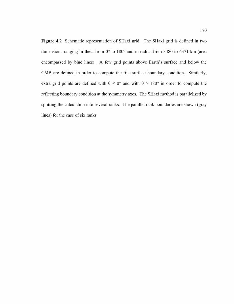
170

Figure 4.2 Schematic representation of SHaxi grid. The SHaxi grid is defined in two

dimensions ranging in theta from 0° to 180° and in radius from 3480 to 6371 km (area

encompassed by blue lines). A few grid points above Earth’s surface and below the

CMB are defined in order to compute the free surface boundary condition. Similarly,

extra grid points are defined with θ < 0° and with θ > 180° in order to compute the

reflecting boundary condition at the symmetry axes. The SHaxi method is parallelized by

splitting the calculation into several ranks. The parallel rank boundaries are shown (gray

lines) for the case of six ranks.

171

Figure 4.3 Detail of SHaxi grid. Location of velocity (vφ) and stress (σrφ and σθφ) grid

points in the SHaxi staggered grid.

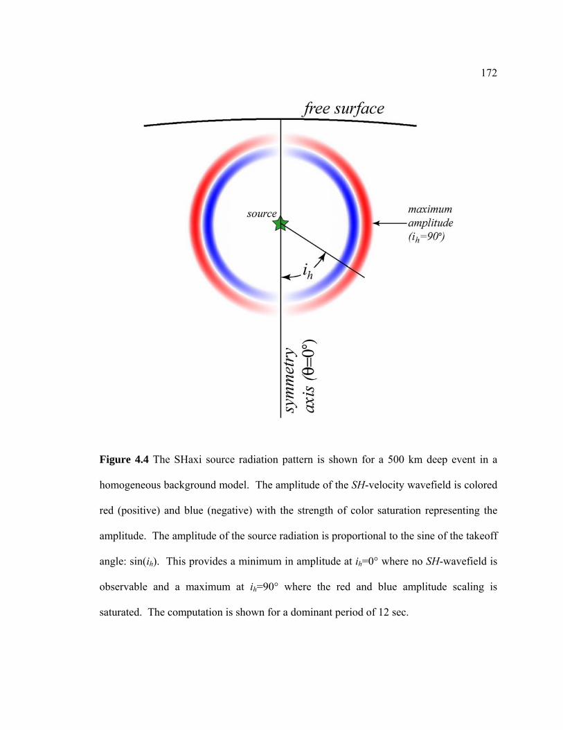
172

Figure 4.4 The SHaxi source radiation pattern is shown for a 500 km deep event in a

homogeneous background model. The amplitude of the SH-velocity wavefield is colored

red (positive) and blue (negative) with the strength of color saturation representing the

amplitude. The amplitude of the source radiation is proportional to the sine of the takeoff

angle: sin(ih). This provides a minimum in amplitude at ih=0° where no SH-wavefield is

observable and a maximum at ih=90° where the red and blue amplitude scaling is

saturated. The computation is shown for a dominant period of 12 sec.

173

Figure 4.5 Hypothetical low- and high- velocity anomaly (red and blue filled areas

respectively) placed onto the 2-D SHaxi grid. The corresponding 3-D axi-symmetric

velocity structure is shown in Figure 4.6.

174

Figure 4.6 Corresponding 3-D axi-symmetric structure of velocity anomalies placed on

grid of Figure 4.5.

175

176

Figure 4.7 The SH-velocity wavefield is shown for three snapshots (simulation time of

250, 500, and 750 seconds) of a SHaxi simulation for the PREM model. Computation is

for a 500 km event depth. Wavefield is shown for a dominant period of 20 sec. Major

seismic phases are labeled with double sided arrows.

177

178

Figure 4.8 PREM tangential component displacement synthetic seismograms.

Seismograms are aligned and normalized to unity on the S arrival. Computation for a 500

km deep source with 5 sec dominant period. Red lines show PREM predicted arrival

times for select phases.

179

Figure 4.9 Random seed matrices (θ) scaled on the interval [0,2π].

180

Figure 4.10 Bessel functions of the second kind. Panel a displays integer order Bessel

functions. The von Karman autocorrelation function uses non-integer order Bessel

functions with order (m) between 0.0 and 0.5 (panel b).

181

Figure 4.11 Autocorrelation functions shown in 1-D for a 32 km autocorrelation length.

The shape of the von Karman autocorrelation function is given for order m=0.0. The

peak amplitude is normalized to unity for each autocorrelation function.

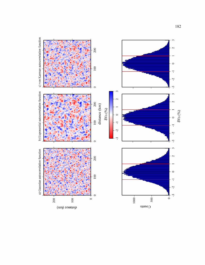
182

183

Figure 4.12 Three realizations of isotropic random media using the same initial random

seed matrix. The top row shows the realization of the S-wave velocity perturbation for

three types of autocorrelation functions. The random media is constructed with an

autocorrelation length of 16 km and a RMS velocity perturbation of 1%. The bottom row

shows the frequency histogram of the three realizations of the first row. In each case the

histogram is Gaussian distributed. The red lines show the region encompassing 1

standard deviation of the velocity perturbation. Velocity perturbations are clipped at

±3% in order to avoid extreme perturbations that may affect the finite difference

simulations stability.

184

Figure 4.13 Power spectra of random media shown in Figure 4.11. The von Karman

type autocorrelation function (ACF) shows the most roughness, as it decays the slowest at

shorter wavelengths. The Gaussian ACF displays the smoothest variation (compare with

Fig. 4.11) as indicated by the fastest decay to shorter wavelengths.

185

186

Figure 4.14 Three realizations of anisotropic random media computed for a von Karman

autocorrelation function. The same random seed is used in each case. The

autocorrelation lengths in the x- and y- directions (alx and aly respectively) are listed

above each panel.

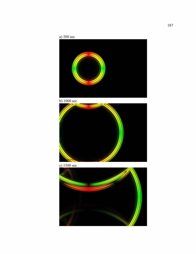
187

188

Figure 4.15 Wave propagation in a homogeneous media produced with E3D.

Computation is for a 1 sec dominant period explosion source placed at 40 km depth and

40 km away from the left grid boundary. A Ricker wavelet is used for the source-time

function. The homogeneous background model has the properties: VS=4.0 km/sec;

VP=5.0 km/sec; density=3.0 g/cm3. The arrival amplitudes are scaled showing red on the

vertical component and green on the horizontal component. The final snapshot (panel c)

displays artificial reflections from an imperfect radiating boundary layer. Also, the

conversion from P-to-S at the free surface reflection (top edge of grid) is observed in

panel c. Total grid dimensions are 80 × 120 km.

189

190

Figure 4.16 Three snapshots of wave propagations through random media are shown.

The model is the homogeneous model of Figure 4.15 with 3% RMS P-wave velocity

perturbations applied to the model. A von Karman autocorrelation function with 1 km

autocorrelation length is used to construct the random media. As opposed to purely

homogeneous case of Fig. 4.15 strong coda development is observed as a result of the

random velocity perturbations. The source and grid parameters are the same as in Fig.

4.15.

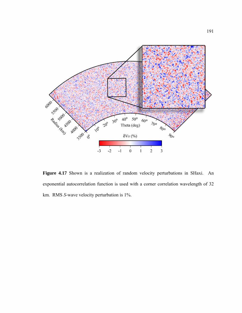
191

Figure 4.17 Shown is a realization of random velocity perturbations in SHaxi. An

exponential autocorrelation function is used with a corner correlation wavelength of 32

km. RMS S-wave velocity perturbation is 1%.

192

Figure 4.18 Detail of representation of random media in SHaxi. Because of axi-

symmetry random velocity perturbations are anisotropic (e.g., see Fig. 4.14) with the

perturbation being stretched in the φ-direction. The realization shown is for a 32 km

autocorrelation length and an exponential autocorrelation function.

193

Figure 4.19 Frequency dependence of scattering. Shown are displacement synthetics for

PREM (dashed line) and for a random media with a Gaussian autocorrelation function

(solid line) created with RMS velocity perturbation of 3% and 16 km autocorrelation

length superimposed on PREM. Seismograms are normalized to unity on the S arrival.

194

Figure 4.20 The dependence of autocorrelation length (ACL) on SH-wave envelopes.

Envelopes of displacement seismograms are shown for the PREM model (black line) and

for the PREM model with three realizations of random S-wave velocity perturbations

applied. The perturbations are produced for a Gaussian autocorrelation function with 3%

RMS velocity perturbations. Envelopes are shown for random perturbations with ACL’s

of 8 km (blue), 16 km (green) and 32 km (red).

CHAPTER 5

3-D SEISMIC IMAGING OF THE D" REGION BENEATH THE COCOS PLATE

Michael S. Thorne1, Thorne Lay2, Edward J. Garnero1, Gunnar Jahnke3,4, Heiner Igel3

1Department of Geological Sciences, Arizona State University, Tempe, AZ 85287-1404, USA. E-mail: mthorne@asu.edu2Department of Earth Sciences, University of California Santa Cruz, Santa Cruz, CA 95064, USA. 3Department of Earth and Environmental Sciences, Ludwig Maximilians Universität, Theresienstrasse 41, 80333 Munich, Germany. 4now at: Federal Institute of Geosciences and Natural Resources, Stilleweg 2, 30655 Hanover, Germany. SUMMARY

We use a 3-D axi-symmetric finite difference algorithm to model SH-wave propagation

through cross-sections of 3-D lower mantle models beneath the Cocos Plate derived from

recent data analyses. Synthetic seismograms with dominant periods as short as 4 sec are

computed for several models: (1) a D" reflector 264 km above the CMB with laterally

varying S-wave velocity increases of 0.9% to 2.6%, based on localized structures from a

1-D double-array stacking method; (2) an undulating D" reflector with large topography

and uniform velocity increase obtained using a 3-D migration method; and (3) cross-

sections through the 3-D mantle S-wave velocity tomography model TXBW. We apply

double-array stacking to assess model predictions of data. Of the models explored, the S-

wave tomography model TXBW displays the best overall agreement with data. The

undulating reflector produces a double Scd arrival that may be useful in future studies for

distinguishing between D" volumetric heterogeneity and D" discontinuity topography. 3-

D model predictions show waveform variability not observed in 1-D model predictions. It

is challenging to predict 3-D structure based on localized 1-D models when lateral

structural variations are on the order of a few wavelengths of the energy used,

particularly for the grazing geometry of our data. Iterative approaches of computing 3-D

196

synthetic seismograms and adjusting 3-D model characteristics by considering path

integral effects are necessary to accurately model fine-scale D" structure.

5.1 Introduction

5.1.1 Lower Mantle Discontinuities

Ever since the designation of the D" region (Bullen 1949), which consists of

heterogeneous velocity structure in the lowermost 200-300 km of the mantle, researchers

have sought to characterize the detailed nature of this boundary layer. The mechanisms

responsible for D" heterogeneity, manifested in strong arrival time fluctuations of seismic

phases sampling the region, are still poorly constrained. It is important to characterize

the D" region because its role as a major internal thermal boundary layer of Earth affects

many disciplines, including mineral physics, global geodynamics, geochemistry, and

geomagnetism (see Lay et al. 2004a for a review). The existence of a D" shear velocity

discontinuity, discovered by Lay & Helmberger (1983), has added further complexity to

creating a detailed picture of the D" region.

Only a handful of seismological techniques directly detect the D" discontinuity.

The discontinuity is most commonly detected by observations of a travel-time triplication

in S- and/or P- waves bottoming in the lower mantle. The structure has also been

detected by observations of a strong arrival in the coda of PKKPAB (Rost & Revenaugh

2003). Studies of differential travel times between pairs of seismic phases (e.g., ScS-S,

PcP-P, PKKPAB-PKKPDF) support the presence of a relatively abrupt increase in deep

mantle wave-speeds in the lowermost mantle (e.g., Creager & Jordan 1986; Woodward &

197

Masters 1991; Zhu & Wysession 1997). Although the differential travel time studies are

compatible with a D" discontinuity, they do not resolve its presence.

During the past two decades, the D" discontinuity has been detected in numerous

seismic investigations (see Wysession et al. 1998 for a review). These studies have

characterized the D" discontinuity as being a sharp P- and/or S- wave velocity (VP and/or

VS) increase (~0.5 to 3.0% for VP and ~0.9 to 3.0% for VS) ranging in height from 150 to

350 km above the core-mantle boundary (CMB) with an average height of 250 km.

The P-wave observations most convincingly associated with a D" discontinuity

are for paths beneath northwestern Siberia (e.g., Weber & Davis 1990; Houard & Nataf

1993). Other studies using P-wave data fail to find strong evidence for the discontinuity

at many locations (e.g., Ding & Helmberger 1997). However, a lack of observations of

P-wave reflections does not necessarily indicate non-existence of a velocity increase in

D". For example, the sharpness, or depth extent, of the boundary plays an important role

in its reflectivity. At grazing angles, where the wavefield triplicates, a velocity increase

spread out over roughly 100 km can match most triplication data as accurately as for a

sharp discontinuity (e.g., Young & Lay 1987; Gaherty & Lay 1992). However; pre-

critical and high-frequency P-waves will be only weakly reflected by such a gradient

increase. An undulating boundary may produce intermittent reflections or scattering that

confuse detections of reflections. Additionally, a relatively low amplitude VP jump at the

D" discontinuity appears to be common, yielding reflections below the detection limit of

routine seismic techniques. In general, past studies have not established whether a D" P-

wave velocity discontinuity is ubiquitous or intermittent.

198

In contrast, S-wave reflections from a D" discontinuity are more commonly

observed. A number of studies have revealed three regions of the deep mantle where the

existence of a D" S-wave velocity discontinuity is particularly well supported by S-wave

observations. These three regions are:

1. Beneath Siberia (e.g., Lay & Helmberger 1983; Weber & Davis 1990; Gaherty

& Lay 1992; Weber 1993; Garnero & Lay 1997; Valenzuela & Wysession 1998;

Thomas et al. 2004b),

2. Beneath Alaska (e.g., Lay & Helmberger 1983; Young & Lay 1990; Lay &

Young 1991; Kendall & Shearer 1994; Matzel et al. 1996; Garnero & Lay 1997;

Lay et al. 1997), and

3. Beneath Central America (e.g., Lay & Helmberger 1983; Zhang & Lay 1984;

Kendall & Shearer 1994; Kendall & Nangini 1996; Ding & Helmberger 1997;

Reasoner & Revenaugh 1999; Ni et al. 2000; Garnero & Lay 2003; Lay et al.

2004b; Thomas et al. 2004a; Hutko et al. 2005).

Some locations in the deep mantle where seismic observations do not show evidence for

a shear wave discontinuity are adjacent to regions where observations do indicate the

presence of a discontinuity. Explanations of why the discontinuity may appear or

disappear over small spatial scales (e.g., < 100 km Lay et al. 2004b) are still debated.

Strong topographic relief on the discontinuity and/or rapid 3-D velocity variations

beneath the discontinuity have been invoked as possible explanations (e.g., Kendall &

Nangini 1996; Thomas et al. 2004a).

199

Additional studies using S-waves have shown evidence for the discontinuity

beneath the Central Pacific (Garnero et al. 1993; Avants et al. 2005). This has motivated

speculation that the feature is global (e.g., Sidorin et al. 1999). Nevertheless, further

probing of the deep mantle, especially under the Southern Pacific and Atlantic Ocean

regions, is needed before the lateral extent of the feature can be ascertained.

5.1.2 S-wave Triplication Behavior

Because the D" discontinuity increase for VS appears to be greater than for VP,

studies utilizing triplications in the S-wave field have been the preferred method for

detecting the discontinuity. In this paper we restrict our attention to S-waves observed on

transverse component (SH) recordings at epicentral distances ranging from roughly 70º to

85º. Fig. 5.1 shows synthetic SH displacement seismograms computed using a finite

difference axi-symmetric method for SH-waves (SHaxi). This method is described in

(Jahnke et al. 2005) and is used to compute synthetic seismograms for D" discontinuity

models.

In Fig. 5.1 synthetic seismograms for the PREM (Dziewonski & Anderson 1981)

shear velocity structure, which does not contain a D" discontinuity, are shown with dotted

lines. Synthetic seismograms for a D" discontinuity model with a 1.3% VS increase

(relative to PREM) 264 km above the CMB are shown in black. Neither model has

crustal layers, as discussed below. Synthetics for the discontinuity model exhibit a travel-

time triplication with extra arrivals between S and ScS. We use the nomenclature of Lay

& Helmberger (1983) to describe the triplication phases labeled in Fig 5.1. The direct S-

200

wave turning above the discontinuity is termed Sab whereas the S-wave energy turning

below the discontinuity is termed Scd. Sbc denotes arrivals reflecting off the

discontinuity. The post-critical Sbc arrival is progressively phase shifted, producing a

small negative overshoot of the combined Scd + Sbc arrival. In Fig. 5.1 distinct Scd and

Sbc arrivals are discernible at larger distances; however the Scd and Sbc arrivals are

generally not separately distinguishable in broadband data. Hence, we refer to the

combined (Scd + Sbc) arrival as SdS. Most studies reference SdS travel-times and

amplitudes to ScS (also shown in Fig. 5.1). Because the synthetics shown in Fig. 5.1

were created for a 500 km deep source, the seismic phase s400S, an underside reflection

from the 400 km discontinuity above the source, is also observed. The amplitude of

s400S is usually too low to be observed in broadband data without stacking records (e.g.,

Flanagan & Shearer 1998).

Fig. 5.2 shows the ray path geometry of the seismic phases in Fig. 5.1 for a

receiver at an epicentral distance of 75º. The ray path geometry is for the same

discontinuity model used to create the synthetic seismograms in Fig. 5.1. Also shown in

Fig. 5.2 is the SH- velocity wavefield at one instance in time through a cross-section of

the Earth computed with the SHaxi method. The relationship between spherical wave

fronts and geometrical rays, which are perpendicular to the wave fronts, can be seen.

Infinite frequency ray paths are useful for visualizing the path that seismic energy takes

through the mantle, however, the seismic energy interaction with Earth structure

surrounding the geometric ray must be considered because it also contributes energy to

the seismic phases recorded at the surface (e.g., Dahlen et al. 2000).

201

5.1.3 Study region and objectives

The D" discontinuity beneath the Central American region has been investigated

extensively because of excellent data coverage provided by South American events and

North American receivers. Three recent studies have focused on mapping the D"

discontinuity structure in 3-D beneath the Cocos Plate subset of the Central American

region (Lay et al. 2004b; Thomas et al. 2004a; Hutko et al. 2005). A recent tomographic

inversion including SdS arrivals has also imaged the lower 500 km of the mantle beneath

Central America (Hung et al. 2005). These regional studies have produced models for

the structure of the discontinuity in the Cocos Plate region and will be discussed in detail

in Section 3.

The variability in seismic differential travel-time (e.g., ScS-Scd or Scd-Sab

differential travel-times – referred to hereafter as TScS-Scd and TScd-Sab respectively) or

amplitude ratio (e.g., Scd/ScS) observations relative to optimal 1-D model predictions

indicate the presence of 3-D D" structure (e.g., Lay & Helmberger 1983; Kendall &

Nangini 1996). Because D" discontinuity topography and VS heterogeneity are both

likely to be 3-D in nature (e.g., Tackley 2000; Farnetani & Samuel 2005), there are major

challenges in resolving discontinuity topography from surrounding volumetric velocity

heterogeneity. Moreover, many D" discontinuity structures have been inferred based on

using localized 1-D processing techniques, without it being clear how to generalize those

models to 3-D structures. This is particularly problematic for triplication arrivals that

graze the deep mantle, with extensive horizontal averaging of the structure. 3-D models

have been obtained using migration approaches that assume homogeneous reference

202

structures and point-scattering assumptions, which intrinsically bias the model images.

Tomography methods usually do not account for abrupt velocity discontinuities, and

incur errors by incorrect back-projection of travel-times on incorrect raypaths.

In order to progress from 1-D processing and modeling techniques that use

simplifying assumptions for 3-D modeling, seismologists must use advanced synthetic

seismogram techniques. Numerical techniques for computing synthetic seismograms in 2-

or 3-D are now becoming practical because of the recent availability and processing

power of cluster computing. In this paper, we produce 3-D synthetic seismograms for our

versions of 3-D models based on various D" discontinuity modeling results beneath the

Cocos Plate. We also create synthetic seismograms through cross-sections of a recent S-

wave tomography models (Grand 2002). The models we construct and compute

synthetics for are summarized in Table 5.1. We compare waveforms and travel-time

differentials from the computed synthetic seismograms with each other and with

broadband data used in the studies of Lay et al. (2004b) and Thomas et al. (2004a).

Furthermore, we analyze the limits of using localized 1-D processing techniques and

lateral interpolations to infer 3-D D" discontinuity structure.

5.2 3-D axi-symmetric finite difference method and verification

Constraining models of 3-D D" structure requires computation of synthetic

seismograms for 3-D geometries (hereafter referred to as 3-D synthetic seismograms) for

comparison to original data. This also allows an assessment of if and how localized 1-D

modeling results or migration methods should be extrapolated to predict actual 3-D

structure. We use the 3-D axi-symmetric finite difference method (SHaxi) (based after

203

Igel & Weber 1995, 1996; and extended in Jahnke et al. 2005) to explore the 3-D model

extrapolations based on recent models of heterogeneous D" structure beneath the Cocos

Plate obtained from several distinct procedures. This is the first application of the SHaxi

method to original data.

The SHaxi method does not incorporate full 3-D Earth models as in some other

numerical techniques (e.g., the spectral element method of Komatitsch & Tromp 2002).

Instead the model defined on a grid in the vertical plane containing the great circle arc is

expanded to 3-D by (virtually) rotating the grid around the vertical axis. As a

consequence the computation on a 2-D grid provides seismogram with the correct

geometrical spreading, but only for axi-symmetric geometries. Nonetheless, this axi-

symmetric method has several advantages for computing synthetic seismograms.

Because it computes the wave field on a 2-D grid, synthetic seismograms can be

generated for much shorter dominant periods (e.g., down to 1 sec) than with full 3-D

techniques. SHaxi also maintains the correct 3-D geometrical spreading, which is an

advantage over purely 2-D techniques that do not.

The main restriction in using the SHaxi method is that structures incorporated on

the 2-D axi-symmetric grid act as 3-D ring-like structures (see Jahnke et al. 2005). This

makes it impossible to model focusing and defocusing effects due to variations off the

great circle plane. Additionally the source acts as a strike-slip with a fixed SH source

radiation pattern proportional to the sine of the takeoff angle. This fixed radiation pattern

makes direct comparison of amplitudes between synthetics and data from arbitrary

204

oriented sources slightly complicated. In this study we are primarily concerned with

differential travel time effects and we place less emphasis on amplitude effects.

In order to produce synthetic seismograms at relatively high frequencies we used

16 nodes (128 processors) of the Hitachi SR8000 super computer at the Leibniz-

Rechenzentrum, Munich, Germany. These computations require 42,000 (lateral) × 6,000

(radial) finite difference grid-points. This grid spacing corresponds to roughly 0.5 km

between grid-points radially, and varies between 0.5 km (Earth’s surface) and 0.25 km

(CMB) laterally. Calculations are run to 1700.0 seconds of simulation time, which takes

approximately 24 hours to compute. For these input parameters, synthetic seismograms

with a dominant period of 4 sec are produced. This is suitable for comparisons with our

SH observations which have been low-pass filtered with a cut-off of 3.3 sec.

In order to ensure that our computations are accurate for the time and epicentral

distance windows used in this study, we used the Gemini (Greens Function of the Earth

by Minor Integration) method of Friederich & Dalkolmo (1995) to compute 1-D PREM

synthetics for comparison to our finite-difference results. The window containing Sab

and ScS that we use starts 20 sec before and ends 100 sec after the Sab arrival in

epicentral distance ranging from 70º – 85º. The Gemini method was chosen because it

has previously been used for verification of other synthetic seismogram techniques (Igel

et al. 2000). We produced 10 sec dominant period synthetics with the Gemini method for

use in our comparisons. Overlaying individual traces display excellent agreement

between the SHaxi and Gemini methods, as demonstrated by a minimum cross-

correlation coefficient between records of 0.9982 at 85º.

205

In synthetics created for PREM [Supplemental Fig. 6A], crustal and mid-crustal

reverberations interfere with the SdS arrival. The average crustal structure represented in

PREM is not a realistic estimate of the complex crustal structure beneath southern

California recording stations (e.g., Zhu & Kanamori 2000). In order to compare our

synthetics to data from southern California stations, we remove the crustal layers from

PREM before computing synthetic seismograms.

5.3 Study region and model construction

5.3.1 D" structure beneath the Cocos Plate

The D" discontinuity structure beneath the Cocos Plate region has been the focus

of numerous seismological studies. Thomas et al. (2004a) provide a review of these

studies, finding that a D" S-wave velocity discontinuity has been consistently inferred at a

height ranging between 150 – 300 km above the CMB with a velocity increase ranging

from 0.9 – 3.0%. There is little evidence for a corresponding P-wave velocity D"

discontinuity (e.g., Ding & Helmberger 1997; Rost, private communication, 2005) other

than the work of Reasoner & Revenaugh (1999) who stack many short-period signals and

infer a weak reflector (0.5 – 0.6% P-wave velocity increase) about 190 km above the

CMB.

Five recent studies have attempted to assess possible small-scale 2- or 3-D

variability of the D" discontinuity beneath the Cocos Plate. Lay et al. (2004b), Thomas

et al. (2004a), and Hutko et al. (2005) produced D" discontinuity models for the Cocos

Plate region using various stacking and migration methods. We compute synthetic

seismograms through cross-sections of our 3-D constructions of the models produced by

206

Lay et al. (2004b) and Thomas et al. (2004a). Ni et al. (2000) computed synthetic

seismograms through cross-sections of the tomography model of Grand (1994) to

determine whether that shear velocity structure helped to improve 1-D D" discontinuity

models. We similarly compute synthetic seismograms for the most recent tomography

model of Grand (2002) for comparison. Hung et al. (2005) presented a lower mantle

tomography model of the Central American region that overlaps the Cocos Plate region.

However, consideration of the Hung et al. (2005) model suggests that it lacks adequate

data sampling in our study region and we do not analyze it further here. We summarize

below how we produced model cross-sections for use in the SHaxi method, and the

results of comparing data to the resulting 3-D synthetics.

5.3.2 Double-array stacking model

Lay et al. (2004b) analyzed broadband transverse component seismic

seismograms including SdS and ScS arrivals from 14 deep South American events

recorded by Californian regional networks. Fig. 5.3a shows the source-receiver

geometries used. The study employed the double-array stacking technique of Revenaugh

& Meyer (1997) to obtain apparent reflector depths of SdS energy for localized bins of

data with nearby ScS CMB reflection points. Fig. 5.3b shows detailed outlines of the four

geographic bins in which Lay et al. (2004b) grouped their data. SdS energy was detected

in stacks throughout the region, however the area delimited by Bin 2 showed weak SdS

energy and some individual seismic traces did not show clear SdS arrivals between Sab

and ScS, as previously noted by Garnero & Lay (2003). If the shear velocity within the

207

D" layer (i.e., between the D" discontinuity and the CMB) is laterally uniform, the stacks

imply localized topography of the discontinuity ranging over 150 km, in which case the

amplitude variations might arise due to reflection from an undulating reflector. However,

Rokosky et al. (2004) and most mantle tomography models suggest a general south-to-

north increase in D" VS from Bin 1 to Bin 4, based primarily on ScS arrival times. Lay et

al. (2004b) modeled the data using localized 1-D models, allowing the average velocity

in the D" layer to vary as needed to match the amplitude of SdS. They found that the

variations required to match the amplitude kept the depth of the discontinuity almost

constant. Their final model involved a 264 km thick D" layer with varying VS increase

across the D" layer ranging from 0.9 to 2.6%. The resulting structures match the general

trend of the ScS arrival time data, except for the model in Bin 1, which predicts earlier

ScS arrivals than observed. Reconciling the SdS amplitudes and ScS arrival times

requires a model with a large discontinuity about 100 km deeper than in bins to the north.

To create models for use with the SHaxi method based on the localized 1-D

results of Lay et al. (2004b), we construct cross-sections through four average great circle

paths from source clusters to station clusters (Path 1 – Path 4, Fig. 5.3b). These great

circle paths are based on the average event-receiver location for events that have ScS

bounce-points in each of the four geographic bins. For each cross-section, we use PREM

velocities above the D" discontinuity. A brief description of models and their naming

convention are outlined in Table 5.1. We constructed models with two end-member

scenarios: (1) the velocity structure in each bin is block-like (model LAYB)

[Supplemental Fig. 6B]; and (2) the velocity structure is linearly interpolated between the

208

center of each bin (model LAYL). We use the same great circle paths (Paths 1-4) to

construct cross-sections for the models listed in Table 5.1. We note that this process

assumes very localized sensitivity of the 1-D modeling as implied by the fine binning

used; as found below this results in very small scale variations that are at odds with the

intrinsic resolution of the nearly horizontally grazing ray geometry.

5.3.3 Point-scattering migration model

Thomas et al. (2004a) employed a pre-critical point-scattering migration

technique (Thomas et al. 1999) to image the deep mantle beneath the Cocos Plate using

the same data set as Lay et al. (2004b). The imaged model space was roughly 700 km in

length and 150 km wide (study region T shown in Fig. 5.3b). The migration study used

the 1-D background model ak135 (Kennett et al. 1995) to provide travel-times for

stacking windows of seismogram subsets compatible with scattering from a specified 3-D

grid of scattering positions. VS was not allowed to vary laterally, which projects all travel

time variations into apparent scattering locations within the background model. A

smoothed version of the resultant scattering image gives a topographically varying D"

discontinuity surface with a south-to-north increase in discontinuity height above the

CMB from 150 to 300 km. This apparent topography is similar to the double-array

stacking results of Lay et al. (2004b) for a 1-D stacking model. The 150 km increase in

discontinuity height occurs in the center of the image region (near Bin2 of Lay et al.

(2004b)), over a lateral distance of roughly 200 km. The central region, containing the

transition in discontinuity depth, does not reflect strong coherent energy and there is

209

uncertainty in the continuity of the structure. The topography in this model is completely

dependent on the assumption of 1-D background structure.

The migration approach used by Thomas et al. (2004a) does not model the

amplitudes and like all Kirchhoff migrations, simply images a reflector embedded in the

background model without accounting for wave interactions with the structure. In order

to compute synthetic seismograms for this structure, it is necessary to prescribe the VS

increase across the imaged reflector. Previous 1-D modeling efforts for the region

suggested a 2.75% (Lay & Helmberger 1983; Kendall & Nangini 1996) or 2.0% (Ding &

Helmberger 1997) VS increase, but Lay et al. (2004b) suggest the region has strong

lateral variability ranging from 0.9 to 2.6%. As initial estimates, we chose VS increases

of 2.0% (model THOM2.0) and 1.0% (model THOM1.0).

Recent studies of a lower mantle phase transition from magnesium silicate

perovskite to a post-perovskite (ppv) structure indicate that the phase transition should

involve 1.5% VS and 1% density increases (Tsuchiya et al. 2004a), providing a possible

explanation for the D" discontinuity. This phase transition also is predicted to have a

steep Clapeyron slope of ~7-10 MPa K-1 (Oganov & Ono 2004; Tsuchiya et al. 2004b),

which could account for significant topography on the D" discontinuity. Because the

study of Thomas et al. (2004a) suggests rapidly varying topography, as may accompany a

ppv phase transition in the presence of lateral thermal and compositional gradients (e.g.,

Hernlund et al. 2005), we also create synthetic seismograms with 1.5% VS and 1%

density increases (model THOM1.5). Model cross-sections are shown in Supplemental

Fig. 6B for model THOM2.0.

210

5.3.4 Tomography model

A consistent feature of recent S-wave tomography models (e.g., Masters et al.

1996; Kuo et al. 2000; Megnin & Romanowicz 2000; Ritsema & van Heijst 2000; Gu et

al. 2001; Grand 2002) is the presence of relatively high shear velocities beneath the

Central America and Cocos Plate region. Model TXBW (parameterized with 2.5º × 2.5º

bins – roughly 150 km on a side) from Grand (2002) was not developed using triplication

arrivals and resolves longer wavelength structure than models produced by Lay et al.

(2004b) and Thomas et al. (2004a). The reference model for TXBW has relatively high

D" velocities, and the lowest layer (bottom 220 km of the mantle) in model TXBW

contains high VS perturbations (up to ~2.3% increases) relative to PREM beneath the

Cocos Plate, with a general south-to-north velocity increase. This is consistent with the

results of Lay et al. (2004b).

Ni et al. (2000) utilized the WKM method (a modification of the WKBJ method

of Chapman 1978) to produce synthetic seismograms through 2-D cross-sections of

block-style tomography models. As an application of their method, Ni et al. (2000)

produced synthetics through two cross-sections of Grand’s (1994) tomography model,

with great-circle paths passing through the Central American region. Ni et al. (2000)

were not able to observe the SdS phase in Grand’s model for the chosen great-circle paths

without arbitrarily increasing the velocity perturbations in the lowermost layer of Grand’s

model by a factor of 3. Their synthetics then compare favorably to broadband Scd

waveforms of Ding & Helmberger (1997) for the Cocos Plate region.

211

We created four cross-sections through Grand’s most recent tomography model

TXBW (Grand 2002) for synthetic seismogram construction with the SHaxi method. To

create cross-sections, we mapped the heterogeneity in TXBW onto our finite difference

grid using four-point inverse distance weighted interpolation between the VS values given

in the model. Our cross-section through great circle Path 1 (Fig. 5.3) is identical to one

of the cross-sections used in the study of Ni et al. (2000).

Model TXBW is parameterized in layers of blocks with constant S-wave velocity

perturbations (δVS). We observe a noticeable increase in average VS between the two

lowermost layers along each of our reference great-circle paths (Path1: +1.5%; Path 2:

+1.75%; Path 3: +1.75%; Path 4: +2.0% - Supplemental Fig. 6C). Ni et al. (2000)

referenced the heterogeneity in Grand’s tomography model directly to PREM (S. Ni,

private communication, 2005) rather than to the 1-D reference model actually used in

Grand’s inversion. When we use the 1-D reference model of Grand, with its velocity

increase in the lowermost mantle, the tomographic models produces significant SdS

energy from the boundary between the two lowermost layers and we find no need to

arbitrarily enhance the structure [Cross-sections are shown in Supplemental Fig. 6C and

D]. Cross-sections through model TXBW show moderate variation in VS progressing

between Paths 1-2-3-4. The strongest variation in velocity structure is observed between

Path 1 and 4.

5.4 Synthetic seismogram results

We computed synthetic seismograms for each great-circle path through the three

models described in the preceding section. Significant variability in waveform shape and

212

differential travel-times between seismic phases is found in the synthetic seismograms for

the various models, as we discuss below. We consider TScS-Scd and TScS–Sab, Scd/ScS

amplitude ratios, and waveform characteristics between the different predictions.

5.4.1 Models LAYB and LAYL

Synthetic seismograms were computed for models LAYB and LAYL which have

block-like or linearly interpolated VS structures, respectively. Differences in waveform

shape or travel-time of arrivals between LAYB and LAYL are not observable for the 4-s

dominant period of our synthetic seismograms. This is because the geographic bin size

used by Lay et al. (2004b) is small compared with the wavelength of S-wave energy in

the D" region (bins are ~2.5º wide in the great circle arc direction, or ~5 wavelengths of a

4 sec dominant period wave at the CMB). The effect of bin size on TScS-Scd and TScS-Sab

will be discussed in Section 7.

We also compute synthetic seismograms for the 1-D models from Lay et al.

(2004b) to compare with our synthetics for the 3-D interpolation of those models.

Overlaying synthetics for model LAYB with synthetics for the 1-D models illuminates

the 3-D structural effects on waveform shape and timing [Supplemental Fig. 6E]. 3-D

synthetics for model LAYB show simple SdS waveforms, similar to the 1-D predictions,

with TScd-Sab between the 1-D and 3-D models unchanged. However, there exists large

variability in TScS-Scd between the synthetics. This is not unexpected since ScS samples

several bins in the 3-D computation, and thereby averages the laterally varying D"

structure. For example, 3-D predictions for Path 2 of LAYB show reduced TScS-Scd (~1.5

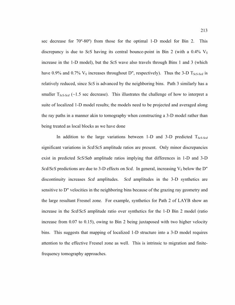
213

sec decrease for 70º-80º) from those for the optimal 1-D model for Bin 2. This

discrepancy is due to ScS having its central bounce-point in Bin 2 (with a 0.4% VS

increase in the 1-D model), but the ScS wave also travels through Bins 1 and 3 (which

have 0.9% and 0.7% VS increases throughout D", respectively). Thus the 3-D TScS-Scd is

relatively reduced, since ScS is advanced by the neighboring bins. Path 3 similarly has a

smaller TScS-Scd (~1.5 sec decrease). This illustrates the challenge of how to interpret a

suite of localized 1-D model results; the models need to be projected and averaged along

the ray paths in a manner akin to tomography when constructing a 3-D model rather than

being treated as local blocks as we have done

In addition to the large variations between 1-D and 3-D predicted TScS-Scd

significant variations in Scd/ScS amplitude ratios are present. Only minor discrepancies

exist in predicted ScS/Sab amplitude ratios implying that differences in 1-D and 3-D

Scd/ScS predictions are due to 3-D effects on Scd. In general, increasing VS below the D"

discontinuity increases Scd amplitudes. Scd amplitudes in the 3-D synthetics are

sensitive to D" velocities in the neighboring bins because of the grazing ray geometry and

the large resultant Fresnel zone. For example, synthetics for Path 2 of LAYB show an

increase in the Scd/ScS amplitude ratio over synthetics for the 1-D Bin 2 model (ratio

increase from 0.07 to 0.15), owing to Bin 2 being juxtaposed with two higher velocity

bins. This suggests that mapping of localized 1-D structure into a 3-D model requires

attention to the effective Fresnel zone as well. This is intrinsic to migration and finite-

frequency tomography approaches.

214

5.4.2 Models THOM1.0, THOM1.5, and THOM2.0

We constructed three models based on Thomas et al. (2004a), one for each of

three distinct D" velocities (see Table 5.1). Larger D" velocity increases produce smaller

TScS-Scd and larger Scd/ScS amplitude ratios, which accounts for the main differences in

synthetics for models THOM1.0, THOM1.5, and THOM2.0. Model THOM1.5 also

included a 1% density increase, which produced indistinguishable synthetics from those

either lacking or containing greater density increases (up to 5%).

Although differences between models THOM1.0 – THOM2.0 are straightforward,

ScS-Scd differential timing and Scd/ScS amplitude ratio effects between Paths 1-4 are

complex [Supplemental Fig. 6F]. Here, we restrict the discussion on variable Path effect

to model THOM2.0.

Along Path 1, the wavefield encounters the deepest D" discontinuity (~130 km

above the CMB) (see Supplemental Fig. 6B). Consequently, TScS-Scd are the smallest.

Along Path 4, the wavefield encounters the shallowest D" discontinuity (~290 km above

the CMB). Although TScS-Scd for Path 4 are greater than for Path 1 (ranging between 1.5

sec larger at 80º to 9 sec larger at 71º), the largest TScS-Scd are sometimes observed for

paths 2 and 3. Along Paths 2 and 3 the wave field encounters the transition from a deep

to shallow D" discontinuity. Three snapshots of the SdS and ScS energy are shown for

Path 3 (Fig. 5.4), which displays the development of a double Scd arrival. In Fig. 5.4(a)

as the wave field interacts with the deepest D" discontinuity structure the Scd phase is

already apparent. 50 sec later the wavefield interacts with the transition from a deep to

shallow discontinuity (Fig. 5.4b), showing more Scd complexity due to multipathing with

215

the shallower and deeper discontinuities. A double Scd arrival is fully developed 50 sec

later, apparent as two distinct Scd peaks in the synthetic seismograms.

At closer epicentral distances (from 70º-72º for Path 3) the Scd arrival originating

from the deeper discontinuity contains higher amplitudes. At the further epicentral

distances (> 72º for path 3) the Scd arrival originating from the shallower discontinuity

contains the higher amplitudes. Arrival times based on Scd peak amplitudes imply an

abrupt jump in TScS-Scd at the epicentral distance where Scd amplitudes from the shallower

discontinuity overtake Scd amplitudes from the deeper discontinuity. For Path 3 a 3 sec

change in TScS-Scd occurs at 72º.

5.4.3 Model TXBW

Fig. 5.5 shows overlain synthetic seismograms computed for model TXBW for

Paths 1 and 4. A clear SdS arrival between Sab and ScS, as well as arrivals between Sab

and SdS caused by crustal reverberations, are apparent for both models. Because of the

layered block-style inversion used to create TXBW, other small arrivals are present from

discontinuous jumps between layers.

Decreases in TScS-Sab (generally < 1 sec on average, but up to 2 sec between paths

1 and 4) are observed moving from Path 1 to 4, due to progressively increasing VS toward

the north in the D" region. This also decreases TScS-Scd (by <1 sec on average between

Path 1 and 4). 3-D structure elsewhere along the paths likely plays an important role in

timing and amplitude anomalies (e.g., Zhao & Lei 2004), but our focus here is on D"

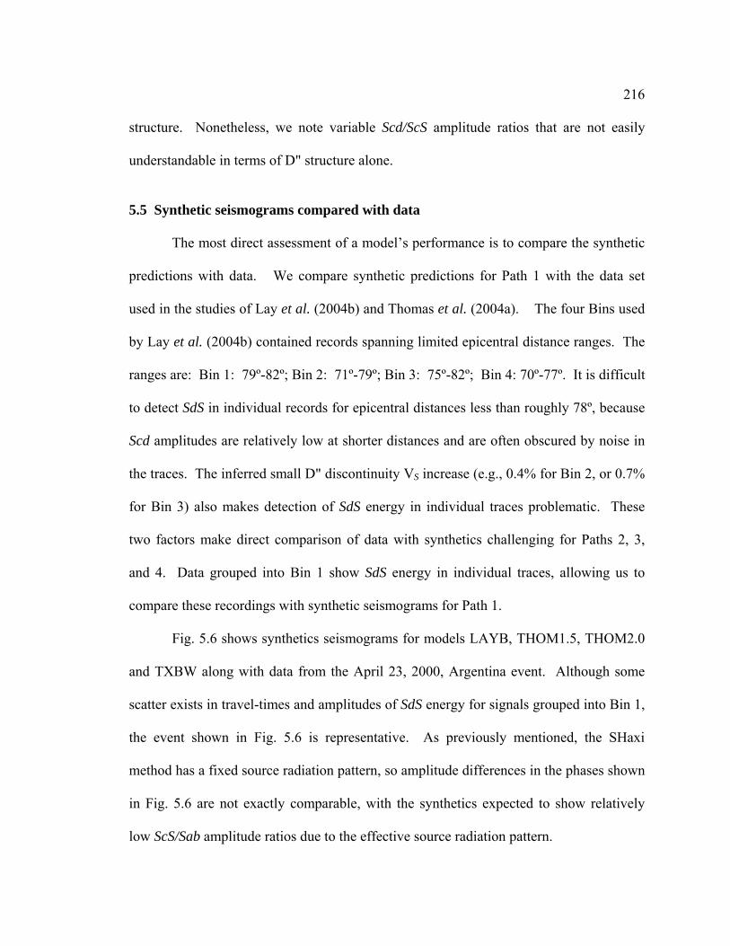
216

structure. Nonetheless, we note variable Scd/ScS amplitude ratios that are not easily

understandable in terms of D" structure alone.

5.5 Synthetic seismograms compared with data

The most direct assessment of a model’s performance is to compare the synthetic

predictions with data. We compare synthetic predictions for Path 1 with the data set

used in the studies of Lay et al. (2004b) and Thomas et al. (2004a). The four Bins used

by Lay et al. (2004b) contained records spanning limited epicentral distance ranges. The

ranges are: Bin 1: 79º-82º; Bin 2: 71º-79º; Bin 3: 75º-82º; Bin 4: 70º-77º. It is difficult

to detect SdS in individual records for epicentral distances less than roughly 78º, because

Scd amplitudes are relatively low at shorter distances and are often obscured by noise in

the traces. The inferred small D" discontinuity VS increase (e.g., 0.4% for Bin 2, or 0.7%

for Bin 3) also makes detection of SdS energy in individual traces problematic. These

two factors make direct comparison of data with synthetics challenging for Paths 2, 3,

and 4. Data grouped into Bin 1 show SdS energy in individual traces, allowing us to

compare these recordings with synthetic seismograms for Path 1.

Fig. 5.6 shows synthetics seismograms for models LAYB, THOM1.5, THOM2.0

and TXBW along with data from the April 23, 2000, Argentina event. Although some

scatter exists in travel-times and amplitudes of SdS energy for signals grouped into Bin 1,

the event shown in Fig. 5.6 is representative. As previously mentioned, the SHaxi

method has a fixed source radiation pattern, so amplitude differences in the phases shown

in Fig. 5.6 are not exactly comparable, with the synthetics expected to show relatively

low ScS/Sab amplitude ratios due to the effective source radiation pattern.

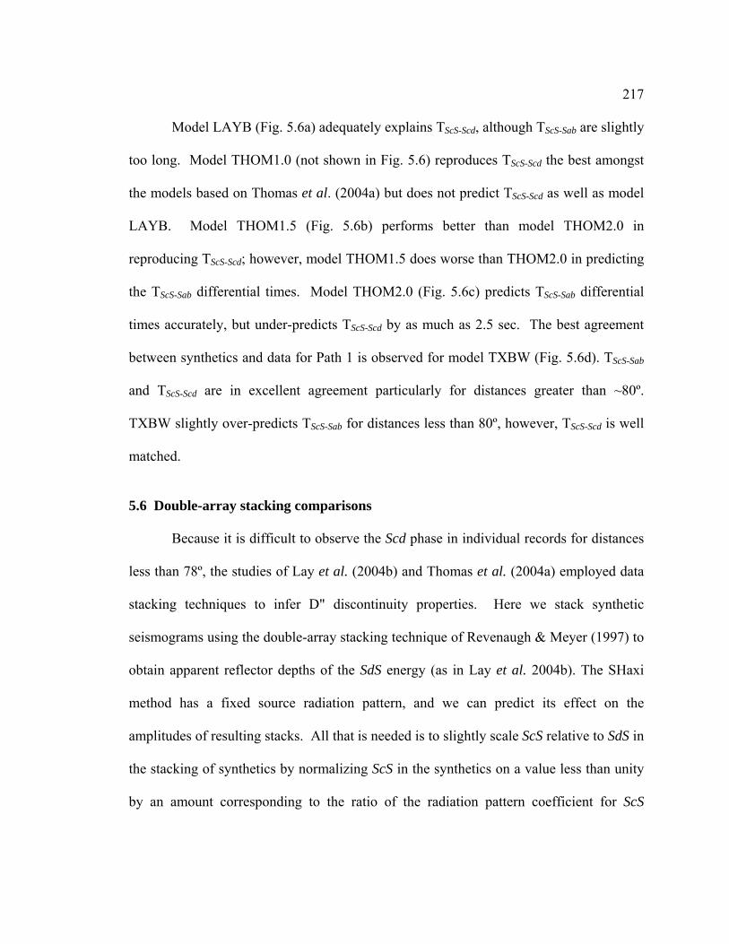
217

Model LAYB (Fig. 5.6a) adequately explains TScS-Scd, although TScS-Sab are slightly

too long. Model THOM1.0 (not shown in Fig. 5.6) reproduces TScS-Scd the best amongst

the models based on Thomas et al. (2004a) but does not predict TScS-Scd as well as model

LAYB. Model THOM1.5 (Fig. 5.6b) performs better than model THOM2.0 in

reproducing TScS-Scd; however, model THOM1.5 does worse than THOM2.0 in predicting

the TScS-Sab differential times. Model THOM2.0 (Fig. 5.6c) predicts TScS-Sab differential

times accurately, but under-predicts TScS-Scd by as much as 2.5 sec. The best agreement

between synthetics and data for Path 1 is observed for model TXBW (Fig. 5.6d). TScS-Sab

and TScS-Scd are in excellent agreement particularly for distances greater than ~80º.

TXBW slightly over-predicts TScS-Sab for distances less than 80º, however, TScS-Scd is well

matched.

5.6 Double-array stacking comparisons

Because it is difficult to observe the Scd phase in individual records for distances

less than 78º, the studies of Lay et al. (2004b) and Thomas et al. (2004a) employed data

stacking techniques to infer D" discontinuity properties. Here we stack synthetic

seismograms using the double-array stacking technique of Revenaugh & Meyer (1997) to

obtain apparent reflector depths of the SdS energy (as in Lay et al. 2004b). The SHaxi

method has a fixed source radiation pattern, and we can predict its effect on the

amplitudes of resulting stacks. All that is needed is to slightly scale ScS relative to SdS in

the stacking of synthetics by normalizing ScS in the synthetics on a value less than unity

by an amount corresponding to the ratio of the radiation pattern coefficient for ScS

218

divided by that for SdS. The actual data are not scaled for source radiation pattern

because for each bin the average SdS/ScS corrections are very close to 1.0.

Fig. 5.7 shows double-array stacks of data compared to synthetic predictions, as

functions of target depth relative to the CMB. PREM is used as the reference stacking

velocity model for both data and synthetics, so apparent SdS reflector depths are biased to

the same extent. We stack synthetics for ranges of epicentral distances that correspond to

those of the corresponding data. ScS energy stacks coherently at the CMB, because the

ScS peaks are aligned on the reference ScS arrival times. SdS energy is clearly apparent

in the data stacks at the apparent depths indicated by the arrows. Saw tooth irregularities

at shallower depths occur as a result of individual waveform truncation before the Sab

arrival. This is done because there tends to be a rise in amplitude of the traces in the Sab

coda.

Double-beam stacking results are summarized in Table 5.2. Model THOM1.0

predicts the D" discontinuity height best, however, it under predicts the SdS/ScS

amplitude ratio most severely. Overall, models LAYB and TXBW predict apparent D"

discontinuity height and SdS/ScS amplitude ratios the best. Model THOM2.0 often

predicts the SdS/ScS amplitude ratio as well as models LAYB and TXBW, but it under

predicts the discontinuity height the most, and the SdS waveform shapes are irregular.

None of the matches are as good as for the 1-D models for each bin obtained by Lay et al.

(2004b).

Although synthetics for model TXBW compare well with data, the fit is not

perfect, especially for Path 2 (Fig. 5.7). D" VS likely varies on shorter scale lengths than

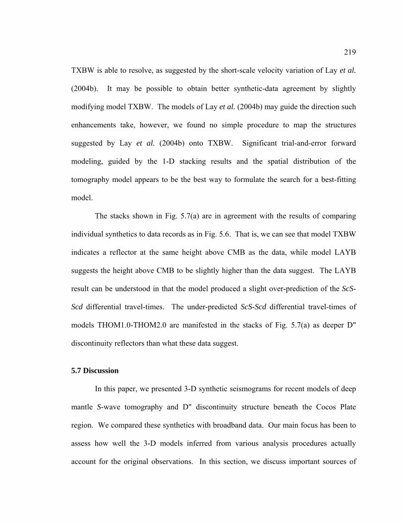
219

TXBW is able to resolve, as suggested by the short-scale velocity variation of Lay et al.

(2004b). It may be possible to obtain better synthetic-data agreement by slightly

modifying model TXBW. The models of Lay et al. (2004b) may guide the direction such

enhancements take, however, we found no simple procedure to map the structures

suggested by Lay et al. (2004b) onto TXBW. Significant trial-and-error forward

modeling, guided by the 1-D stacking results and the spatial distribution of the

tomography model appears to be the best way to formulate the search for a best-fitting

model.

The stacks shown in Fig. 5.7(a) are in agreement with the results of comparing

individual synthetics to data records as in Fig. 5.6. That is, we can see that model TXBW

indicates a reflector at the same height above CMB as the data, while model LAYB

suggests the height above CMB to be slightly higher than the data suggest. The LAYB

result can be understood in that the model produced a slight over-prediction of the ScS-

Scd differential travel-times. The under-predicted ScS-Scd differential travel-times of

models THOM1.0-THOM2.0 are manifested in the stacks of Fig. 5.7(a) as deeper D"

discontinuity reflectors than what these data suggest.

5.7 Discussion

In this paper, we presented 3-D synthetic seismograms for recent models of deep

mantle S-wave tomography and D" discontinuity structure beneath the Cocos Plate

region. We compared these synthetics with broadband data. Our main focus has been to

assess how well the 3-D models inferred from various analysis procedures actually

account for the original observations. In this section, we discuss important sources of

220

uncertainty and difficulties associated with the models for which we computed synthetic

seismograms.

Lay et al. (2004b) produced 1-D models of the D" discontinuity structure with

excellent agreement to data stacks. However, our 3-D synthetics for model LAYB

compared less favorably to data stacks. The main issue here is how best to develop a 3-D

structure from the ‘local’ characterization provided by small bin processing given the

grazing nature of the seismic waves which must laterally average the structure. The SdS

features in the data stacks are remarkably discrete; even small overlap of the bins leads to

appearance of double peaks in the stacks, as noted by Lay et al. (2004b). But the grazing

ray geometry argues that this cannot be interpreted as resolving spatial heterogeneities on

the scale of the actual binning. What is needed is an understanding of the mapping of the

locally characterized wavefield into heterogeneous structure. This is undoubtedly a non-

linear mapping given that volumetric heterogeneity and reflector topography can trade-

off.

We explore the effects of VS heterogeneity wavelength on TScS-Scd and TScS-Sab in

Fig. 5.8. We construct a suite of models with a base model containing a D" discontinuity

at a height of 264 km above the CMB and a VS increase of 2.33%. Synthetic

seismograms are computed for a source 500 km deep at an epicentral distance of 78º.

The ScS bounce-point for this source-receiver geometry is located at 38.12º from the

source. Centered on this ScS bounce-point we introduce a domain with higher VS (+3%

increase). This higher velocity domain is given a width along the great-circle path in

varying multiples of the ScS wavelength for a dominant period of 7 sec (1 wavelength ≈

221

50 km). In Fig. 5.8, the ScS-Sab differential travel times are shown as a function of

domain size for the high velocity region. For TScS-Sab, a domain width of 2-3 wavelengths

already affects the differential travel-times by a few tenths of seconds. However it is not

until a domain width of roughly 30 wavelengths (~1500 km for a 7 sec dominant period

wave) is reached that TScS-Sab converges to the travel-time prediction for a 1-D model with

a 3.0% VS increase beneath the discontinuity. This is consistent with the long path

length of ScS within the D" layer and the large effective Fresnel zone for wide-angle

reflections as indicated in Figure 5.2.

The Bin sizes used in the Lay et al. (2004b) study are on average roughly 3

wavelengths in length along the great circle path. Fig. 5.8 demonstrates that differential

travel-times may be significantly dominated by the neighboring bin structure. ScS-Scd

times suffer a similar lack of path isolation. These experiments argue that 1-D travel time

modeling results are biased if along path lateral variability is shorter scale than about 30-

wavelengths. However, our SdS data clearly display strong variation over distances of

much less than 30-wavelengths, thus 3-D techniques must be employed to reliably map

the required heterogeneous structure. It is unrealistically optimistic to believe that fine

binning resolves fine scale structure when grazing rays are being used; the wave

propagation effects may be spatially rapidly varying but the responsible structure is likely

to be large scale. Since tomography intrinsically distributes path integral effects over

large scale, it can provide a good starting basis for initial modeling, as demonstrated by

Ni et al. (2000) and by the modeling in this paper.

222

We also calculated TScS-Sab and TScS-Scd using 3-D ray tracing for the same model

geometries as used for Fig. 5.8. The 3-D ray tracing solutions coincide with the travel-

times shown in Fig. 5.8 to within a couple tenths of seconds. However, significant

variations between ray tracing and waveform predictions occur when imaging low-

velocity layers.

Paths 2 and 3 of models THOM1.0-2.0 show a rapid transition in D" discontinuity

thickness (e.g., Fig 5.4 and Supplemental Fig. 6B) producing a double Scd peak in the

synthetic predictions. This double Scd peak has not been reported in observations, but

comes to light with the calculation of 3-D synthetic seismograms. Given the possibility

of the post-perovskite phase transition being responsible for the D" discontinuity, it is

interesting to establish whether models with rapid variations in topography can account

for the data. Future efforts seeking to resolve topographic variation on the D"

discontinuity should consider the prediction of a double Scd arrival.

For the SHaxi approach, out of great circle plane variations in D" discontinuity

topography cannot be modeled, so we do not model the exact scattering of energy that the

full 3-D model of Thomas et al. (2004a) would produce. Because our models are axi-

symmetric more SdS energy may be backscattered from the transition from thin to thick

D" layering in models THOM1.0-2.0 than would be scattered in fully 3-D models.

Models THOM1.0-2.0 have relatively small SdS/Scd amplitudes, though we are not able

to constrain the degree of Scd amplitude misfit due to our geometry. Perhaps the

greatest challenge for interpreting migration images is that they do not resolve velocity

contrasts (at least for Kirchhoff point-scattering migrations), and the reflector images are

223

highly dependent on the reference velocity structure. Volumetric heterogeneity as needed

to match ScS arrival times suggests that apparent topography is likely to be incorrect, and

in this case, exaggerated. Thus, the poor agreement of resulting synthetics is not a clear

indication that the models are flawed; the mapping to 3-D may simply be in significant

error. This uncertainty extends to any effort to infer dynamical features based on the

migration images.

If VS gradients perpendicular to our 2-D cross-sections for model TXBW are

insignificant over a distance of a couple of wavelengths our synthetics should be

adequate. Because there was only slight change in our synthetic predictions between

individual paths, lateral variation does appears to be minor for our geometry and full 3-D

synthetics may not be necessary to predict the waveforms. Not having to compute full 3-

D synthetics for the present class of whole Earth tomography models would drastically

save computational resources and time, and is currently feasible using low-cost cluster

computing. We are currently exploring differences between synthetics computed for

tomography models with fully 3-D codes and the SHaxi method, which will be reported

on soon.

5.8 Conclusions

We have demonstrated that important 3-D wavefield effects are predicted for

models of 3-D structure built upon underlying 1-D modeling assumptions. We have

investigated recent models of D" discontinuity structure beneath the Cocos Plate region

using 3-D synthetic seismograms calculated with the finite-difference SHaxi method. We

made synthetic predictions for 3-D models inferred from results of several recent “high

224

resolution” imaging studies, including D" discontinuity mapping by stacking and

migration, and tomographically derived volumetric heterogeneity. We focused our

comparison on seismic phases predominantly used to image D" discontinuity structure: S,

ScS and the intermediate arrival SdS which is present if a high velocity D" layer exists.

We found significant discrepancies between observations and 3-D synthetic predictions,

which highlight the need for 3-D tools in the process of mapping localized imaging

results into 3-D structure. 1-D tools are unable to accurately predict 3-D structure if

structural variations are on the order of wavelength of the energy used; the problem is

particularly severe for grazing ray geometries. 3-D ray tracing techniques may aid in

constructing 3-D models by providing improved reference seismic arrival times.

However, methods utilizing 3-D synthetic seismograms, such as the SHaxi approach, are

better suited for this purpose as important waveform effects can be synthesized. In order

to model fine-scale 3-D D" structure, we believe future efforts should incorporate

methods of synthesizing 3-D seismograms in an iterative approach. Reasonable starting

models may be constructed by migration or double-array stacking techniques, which may

be improved if tomographic models are used as the reference structure. Initial models

can be improved in an iterative fashion by computing 3-D synthetic seismograms,

comparing the synthetics with data, and adjusting the model. However, it will be

challenging to determine the best way to adjust the model in the forward sense, requiring

significant trial and error. In the inverse sense, low cost methods such as SHaxi may

allow reasonable full waveform inversions to be calculated along corridors densely

sampled with data.

225

ACKNOWLEDGEMENTS

Most figures were generated using the Generic Mapping Tools freeware package (Wessel

& Smith 1998). M. T. and E. G. were partially supported by NSF grant EAR-0135119.

T. L. was supported by NSF Grant EAR-0125595. Thanks to the Leibniz Computing

Center, Munich, for access to their computational facilities. Support is also acknowledged

from the German Academic Exchange Service (IQN-Georisk), the German Research

Foundation, and the Human Resources and Mobility Programme of the European Union

(SPICE-Project). The SHaxi source code is openly available at http://www.spice-rtn.org/.

226

REFERENCES

Avants, M. S., Lay, T., Russell S.A., & Garnero, E.J., 2005. Shear-velocity variation

within the D" region beneath the central Pacific, Journal of Geophysical Research - Solid Earth, in review.

Bullen, K. E., 1949. Compressibility-pressure hypothesis and the Earth's interior,

Monthly Notes of the Royal Astronomical Society, Geophysics Supplement, 355-368.

Chapman, C.H., 1978. A new method for computing synthetic seismograms, Geophys. J.

R. astr. Soc., 54, 481-518. Creager, K. C. & Jordan, T. H., 1986. Aspherical structure of the core-mantle boundary

from PKP Travel-Times, Geophysical Research Letters, 13, 1497-1500. Dahlen, F. A., Hung, S. H. & Nolet, G., 2000. Frechet kernels for finite-frequency

traveltimes - I. Theory, Geophysical Journal International, 141, 157-174. Ding, X. M. & Helmberger, D. V., 1997. Modelling D'' structure beneath Central

America with broadband seismic data, Physics of the Earth and Planetary Interiors, 101, 245-270.

Dziewonski, A. M. & Anderson, D. L., 1981. Preliminary Reference Earth Model,

Physics of the Earth and Planetary Interiors, 25, 297-356. Farnetani, C. G., and H. Samuel, 2005. Beyond the thermal plume paradigm, Geophys.

Res. Lett., 32, No.7, L07311, 10.1029/2005GL022360. Flanagan, M. P. & Shearer, P. M., 1998. Topography on the 410-km seismic velocity

discontinuity near subduction zones from stacking of sS, sP, and pP precursors, Journal of Geophysical Research-Solid Earth, 103, 21165-21182.

Friederich, W. & Dalkolmo, J., 1995. Complete synthetic seismograms for a spherically

symmetrical Earth by a numerical computation of the Greens-function in the frequency-domain, Geophysical Journal International, 122, 537-550.

Gaherty, J. B. & Lay, T., 1992. Investigation of laterally heterogeneous shear velocity

structure in D'' beneath Eurasia, Journal of Geophysical Research-Solid Earth, 97, 417-435.

227

Garnero, E. J., Helmberger, D. V. & Grand, S., 1993. Preliminary evidence for a lower mantle shear-wave velocity discontinuity beneath the Central Pacific, Physics of the Earth and Planetary Interiors, 79, 335-347.

Garnero, E. J. & Lay, T., 1997. Lateral variations in lowermost mantle shear wave

anisotropy beneath the north Pacific and Alaska, Journal of Geophysical Research-Solid Earth, 102, 8121-8135.

Garnero, E. J. & Lay, T., 2003. D '' shear velocity heterogeneity, anisotropy and

discontinuity structure beneath the Caribbean and Central America, Physics of the Earth and Planetary Interiors, 140, 219-242.

Grand, S. P., 1994. Mantle shear structure beneath the America and surrounding oceans,

Journal of Geophysical Research-Solid Earth, 99, 11591-11621. Grand, S. P., 2002. Mantle shear-wave tomography and the fate of subducted slabs,

Philosophical Transactions of the Royal Society of London Series a-Mathematical Physical and Engineering Sciences, 360, 2475-2491.

Gu, Y. J., Dziewonski, A. M., Su, W. J. & Ekstrom, G., 2001. Models of the mantle shear

velocity and discontinuities in the pattern of lateral heterogeneities, Journal of Geophysical Research-Solid Earth, 106, 11169-11199.

Hernlund, J.W, C. Thomas, P.J. Tackley, A doubling of the post-perovskite phase

boundary and structure of the Earth's lowermost mantle, Nature, 434, 883-886, 2005.

Houard, S. & Nataf, H. C., 1993. Laterally varying reflector at the top of D'' beneath

Northern Siberia, Geophysical Journal International, 115, 168-182. Hung, S.-H., Garnero, E., Chiao, L.-Y., Lay, T. & Kuo, B. Y., 2005. Finite frequency

tomography of D" shear velocity heterogeneity beneath the Caribbean, Journal of Geophysical Research, 110, doi: 10.1029/2004JB003373.

Hutko, A., Lay, T., Garnero, E. & Revenaugh, J. R., 2005. A folded slab at the core-

mantle boundary beneath the Cocos Plate imaged by Kirchoff migration, Nature, submitted.

Igel, H. & Weber, M., 1995. SH-wave propagation in the whole mantle using high-order

finite differences, Geophys. Res. Let., 22, 731-734. Igel, H. & Weber, M., 1996. P-SV wave propagation in the Earth's mantle using finite

differences: Application to heterogeneous lowermost mantle structure, Geophys. Res. Let., 23, 415-418.

228

Igel, H., Takeuchi, N., Geller, R. J., Megnin, C., Bunge, H. P., Clevede, E., Dalkolmo, J. & Romanowicz, B., 2000. The COSY Project: verification of global seismic modeling algorithms, Physics of the Earth and Planetary Interiors, 119, 3-23.

Jahnke, G., Thorne, M.S., Cochard, A., & Igel, H., 2005. Global SH wave propagation

with an axi-symmetric finite-difference scheme, Geophysical Journal International, submitted 2005.

Kendall, J. M. & Shearer, P. M., 1994. Lateral Variations in D'' thickness from long-

period shear-wave data, Journal of Geophysical Research-Solid Earth, 99, 11575-11590.

Kendall, J. M. & Nangini, C., 1996. Lateral variations in D'' below the Caribbean,

Geophysical Research Letters, 23, 399-402. Kennett, B. L. N., Engdahl, E. R. & Buland, R., 1995. Constraints on seismic velocities

in the Earth from travel-times, Geophysical Journal International, 122, 108-124. Komatitsch, D. & Tromp, J., 2002. Spectral-element simulations of global seismic wave

propagation - I. Validation, Geophysical Journal International, 149, 390-412. Kuo, B. Y., Garnero, E. J. & Lay, T., 2000. Tomographic inversion of S-SKS times for

shear velocity heterogeneity in D '': Degree 12 and hybrid models, Journal of Geophysical Research-Solid Earth, 105, 28139-28157.

Lay, T. & Helmberger, D. V., 1983. A lower mantle S-wave triplication and the shear

velocity structure of D'', Geophysical Journal of the Royal Astronomical Society, 75, 799-837.

Lay, T. & Young, C. J., 1991. Analysis of seismic SV waves in the core's penumbra,

Geophysical Research Letters, 18, 1373-1376. Lay, T., Garnero, E. J., Young, C. J. & Gaherty, J. B., 1997. Scale lengths of shear

velocity heterogeneity at the base of the mantle from S wave differential travel times, Journal of Geophysical Research-Solid Earth, 102, 9887-9909.

Lay, T., Garnero, E. J. & William, Q., 2004a. Partial melting in a thermo-chemical

boundary layer at the base of the mantle, Physics of the Earth and Planetary Interiors, 146, 441-467.

Lay, T., Garnero, E. J. & Russell, S. A., 2004b. Lateral variation of the D '' discontinuity

beneath the Cocos Plate, Geophysical Research Letters, 31, doi:10.1029/2004GL020300.

229

Masters, G., Johnson, S., Laske, G. & Bolton, H., 1996. A shear-velocity model of the mantle, Philosophical Transactions of the Royal Society of London Series a-Mathematical Physical and Engineering Sciences, 354, 1385-1410.

Matzel, E., Sen, M. K. & Grand, S. P., 1996. Evidence for anisotropy in the deep mantle

beneath Alaska, Geophysical Research Letters, 23, 2417-2420. Megnin, C. & Romanowicz, B., 2000. The three-dimensional shear velocity structure of

the mantle from the inversion of body, surface and higher-mode waveforms, Geophysical Journal International, 143, 709-728.

Ni, S. D., Ding, X. M. & Helmberger, D. V., 2000. Constructing synthetics from deep

earth tomographic models, Geophysical Journal International, 140, 71-82. Oganov, A. R. & Ono, S., 2004. Theoretical and experimental evidence for a post-

perovskite phase of MgSiO3 in Earth's D '' layer, Nature, 430, 445-448. Reasoner, C. & Revenaugh, J., 1999. Short-period P wave constraints on D '' reflectivity,

Journal of Geophysical Research-Solid Earth, 104, 955-961. Revenaugh, J. & Meyer, R., 1997. Seismic evidence of partial melt within a possibly

ubiquitous low-velocity layer at the base of the mantle, Science, 277, 670-673. Ritsema, J. & van Heijst, H.-J., 2000. Seismic imaging of structural heterogeneity in

Earth's mantle: Evidence for Large-Scale Mantle Flow, Science Progress, 83, 243-259.

Rokosky, J. M., Lay, T., Garnero, E. J. & Russell, S. A., 2004. High-resolution

investigation of shear wave anisotropy in D '' beneath the Cocos Plate, Geophysical Research Letters, 31, L07605.

Rost, S. & Revenaugh, J., 2003. Detection of a D '' discontinuity in the south Atlantic

using PKKP, Geophysical Research Letters, 30, 1840. Sidorin, I., Gurnis, M., & Helmberger, D. V., 1999. Evidence for a ubiquitous seismic

discontinuity at the base of the mantle, Science, 286, 1326-1331. Tackley, P.J., 2000. Mantle convection and plate tectonics: Towards an integrated

physical and chemical theory, Science, 288, 2002-2007, 2000. Thomas, C., Weber, M., Wicks, C. W. & Scherbaum, F., 1999. Small scatterers in the

lower mantle observed at German broadband arrays, Journal of Geophysical Research-Solid Earth, 104, 15073-15088.

230

Thomas, C., Garnero, E. J. & Lay, T., 2004a. High-resolution imaging of lowermost mantle structure under the Cocos plate, Journal of Geophysical Research-Solid Earth, 109, doi:10.1029/2004JB003013.

Thomas, C., Kendall, J., Lowman, J., 2004b. Lower-mantle seismic discontinuities and

the thermal morphology of subducted slabs, Earth Planet. Sci. Lett., 225, 105–113.

Tsuchiya, T., Tsuchiya, J., Umemoto, K. & Wentzcovitch, R. A., 2004a. Phase transition

in MgSiO3 perovskite in the earth's lower mantle, Earth and Planetary Science Letters, 224, 241-248.

Tsuchiya, T., Tsuchiya, J., Umemoto, K. & Wentzcovitch, R. M., 2004b. Elasticity of

post-perovskite MgSiO3, Geophysical Research Letters, 31, L14603, doi:10.1029/2004GL020278.

Valenzuela, R. W. & Wysession, M. E., 1998. Illuminating the Base of the Mantle with

Diffracted Waves, in The Core-Mantle Boundary Region, pp. 57-71, ed., Gurnis, M., Wysession, M. E., Knittle, E. & Buffet, B. A., American Geophysical Union, Washington, D.C.

Weber, M. & Davis, J. P., 1990. Evidence of a laterally variable lower mantle structure

from P-waves and S-waves, Geophysical Journal International, 102, 231-255. Weber, M., 1993. P-wave and S-wave reflections from anomalies in the lowermost

mantle, Geophysical Journal International, 115, 183-210. Wessel, P., and W. H. F. Smith, 1998. New, improved version of the Generic Mapping

Tools released, Eos Trans. AGU, 79, 579. Woodward, R. L. & Masters, G., 1991. Lower-mantle structure from ScS-S differential

travel-times, Nature, 352, 231-233. Wysession, M. E., Lay, T., Revenaugh, J., Williams, Q., Garnero, E., Jeanloz, R. &

Kellogg, L. H., 1998. The D" discontinuity and its implications, in The Core-Mantle Boundary Region, pp. 273-297, ed., Gurnis, M., Wysession, M. E., Knittle, E. & Buffet, B. A., American Geophysical Union, Washington, D.C.

Young, C. J. & Lay, T., 1987. Evidence for a shear velocity discontinuity in the lower

mantle beneath India and the Indian-Ocean, Physics of the Earth and Planetary Interiors, 49, 37-53.

Young, C. J. and T. Lay (1990). Multiple phase analysis of the shear velocity structure in

the D" region beneath Alaska, J. Geophys. Res., 95, 17385-17402.

231

Zhang, J. J. & Lay, T., 1984. Investigation of a lower mantle shear-wave triplication using a broad-band array, Geophysical Research Letters, 11, 620-623.

Zhao, D. & Lei, J., 2004. Seismic ray path variations in a 3D global velocity model,

Physics of the Earth and Planetary Interiors, 141, 153-166. Zhu, A. N. & Wysession, M. E., 1997. Mapping global D'' P velocities from ISC PcP-P

differential travel times, Physics of the Earth and Planetary Interiors, 99, 69-82. Zhu, L. P. & Kanamori, H., 2000. Moho depth variation in southern California from

teleseismic receiver functions, Journal of Geophysical Research-Solid Earth, 105, 2969-2980.

232

TABLES

Table 5.1 Models Model Description Model based on: LAYBa Block style bins Lay et al. 2004b LAYLa Linear interpolation between bins Lay et al. 2004b THOM1.0b 1% Vs increase beneath discontinuity Thomas et al. 2004aTHOM1.5b 1.5% Vs & 1% ρ increase beneath discontinuity Thomas et al. 2004aTHOM2.0b 2% Vs increase beneath discontinuity Thomas et al. 2004aTXBW Tomographically derived δVS heterogeneity Grand 2002 aFixed D" thickness, variable D" δVSbVariable D" thickness, fixed D" δVS

233

Table 5.2 D" thickness (km)* from double-beam stacking for data and models

Path Data LAYB THOM1.0 THOM1.5 THOM2.0 TXBW Path 1 160 185 115 95 80 167 Path 2 270 227 234 215 200 210 Path 3 250 196 230 202 182 198 Path 4 220 229 213 193 172 199 *Thickness refers to Scd peak in Fig. 5.7.

234

FIGURES

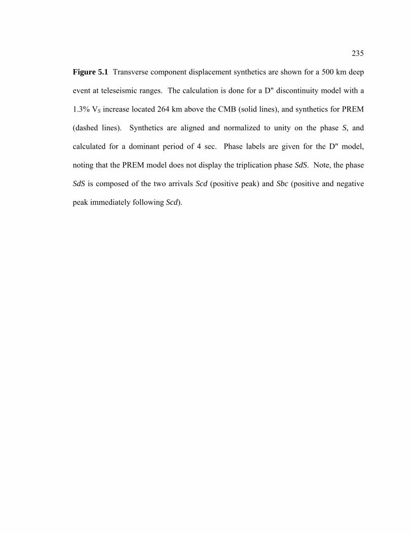
235

Figure 5.1 Transverse component displacement synthetics are shown for a 500 km deep

event at teleseismic ranges. The calculation is done for a D" discontinuity model with a

1.3% VS increase located 264 km above the CMB (solid lines), and synthetics for PREM

(dashed lines). Synthetics are aligned and normalized to unity on the phase S, and

calculated for a dominant period of 4 sec. Phase labels are given for the D" model,

noting that the PREM model does not display the triplication phase SdS. Note, the phase

SdS is composed of the two arrivals Scd (positive peak) and Sbc (positive and negative

peak immediately following Scd).

236

237

Figure 5.2 a) The SH- velocity wave field is shown at propagation time of 600 sec for a

500 km deep event with dominant source period of 6 sec. Selected wave fronts are

labeled with black double-sided arrows. Ray paths are drawn in black for an epicentral

distance of 75º. The calculation is done for the D" discontinuity (indicated with a dashed

green line) model of Fig. 5.1. Non-linear scaling was applied to the wavefield amplitudes

to magnify lower amplitude phases. b) Detail of wavefield shown in panel a. The region

displayed is indicated by a dashed blue box in panel a.

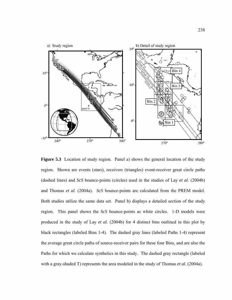
238

Figure 5.3 Location of study region. Panel a) shows the general location of the study

region. Shown are events (stars), receivers (triangles) event-receiver great circle paths

(dashed lines) and ScS bounce-points (circles) used in the studies of Lay et al. (2004b)

and Thomas et al. (2004a). ScS bounce-points are calculated from the PREM model.

Both studies utilize the same data set. Panel b) displays a detailed section of the study

region. This panel shows the ScS bounce-points as white circles. 1-D models were

produced in the study of Lay et al. (2004b) for 4 distinct bins outlined in this plot by

black rectangles (labeled Bins 1-4). The dashed gray lines (labeled Paths 1-4) represent

the average great circle paths of source-receiver pairs for these four Bins, and are also the

Paths for which we calculate synthetics in this study. The dashed gray rectangle (labeled

with a gray-shaded T) represents the area modeled in the study of Thomas et al. (2004a).

239

240

Figure 5.4 Snapshots at three time intervals are shown for model THOM2.0 for Path 3.

The view displayed includes a section of the lower-most mantle between radii 3480 -

4500 km and between epicentral distances 25º - 55º. The amplitude of the SH- velocity

wavefield is shown in red and blue. The top of the D" discontinuity in model THOM2.0

is drawn with a solid black line. Select seismic phases are labeled with double-sided

arrows. These snapshots show the evolution of the wave field as it encounters a D"

discontinuity with topographic variation. The topographic variation is observed to

produce two distinct Scd arrivals.

241

Figure 5.5 Comparison of synthetics for model TXBW for Paths 1 (black) and 4 (gray).

Transverse component displacement synthetics are shown. Synthetics are aligned and

normalized to unity on the phase Sab, and calculated for a dominant period of 4 sec. For

clarity, lines are drawn at the peak SdS and ScS arrival time for Path 1.

242

243

Figure 5.6 Comparison of synthetics created for Path 1 (solid lines) with data (dashed

lines, April 23, 2000 Argentina 600 km deep event). Transverse component

displacement synthetics and data are shown. Data are distance shifted to a source depth

of 500 km. Approximate arrival times (peak amplitude) for the phases Sab, Scd, and ScS

for data are indicated by solid lines so that differences between data and synthetic

differential travel-times can be easily inspected visually. Receiver names are listed to the

right of data traces.

244

Figure 5.7 Stacking results for each Path (1-4) of synthetic prediction and Bin (1-4) of

data are shown. Data stacks from Lay et al. (2004b) are drawn in black. The epicentral

distance range of these data is displayed in the upper right corner of each panel. We

stacked synthetic seismograms for the same epicentral distance range as these data.

245

Figure 5.8 3-D effects of D" lateral VS heterogeneity on TScS–Sab (panel a) and TScS-Scd

(panel b) is shown. These differential travel-times are computed for a D" model with a

constant VS = 7.375 km/sec (+2.33% jump) except in a box centered on the ScS bounce

point for source-receiver epicentral distance of 78º and source depth of 500 km (central

bounce-point = 38.12º). Inside this box the VS is 7.431 km/sec (+3% jump). The D"

thickness is fixed at 264 km corresponding with the study of Lay et al. (2004b). The

width of the inner box is shown on the right axis in km and on the left axis in multiples of

the wavelength of ScS in the box. The wavelength multiples are shown for a ScS

dominant period of 7 sec for which the synthetics were computed.

246

SUPPLEMENTAL FIGURES

247

Supplement 5A Transverse component displacement synthetics are shown. Synthetics

for PREM with a 500 km source depth are drawn in blue. Synthetics are aligned and

normalized to unity on the phase S, and calculated for a dominant period of 4 sec.

Crustal and mid-crustal phases that interfere with the SdS and ScS wavefield are labeled

with green lines. S and ScS are labeled with red lines. The yellow line labels the

underside reflection of the 400 km depth discontinuity in PREM (s400S).

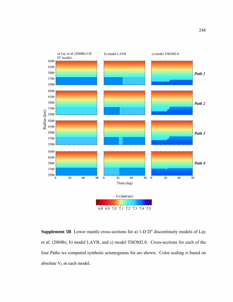
248

Supplement 5B Lower mantle cross-sections for a) 1-D D" discontinuity models of Lay

et al. (2004b), b) model LAYB, and c) model THOM2.0. Cross-sections for each of the

four Paths we computed synthetic seismograms for are shown. Color scaling is based on

absolute VS in each model.

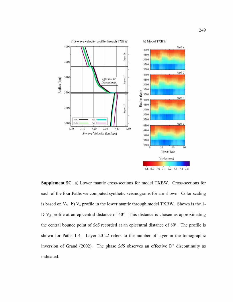
249

Supplement 5C a) Lower mantle cross-sections for model TXBW. Cross-sections for

each of the four Paths we computed synthetic seismograms for are shown. Color scaling

is based on VS. b) VS profile in the lower mantle through model TXBW. Shown is the 1-

D VS profile at an epicentral distance of 40º. This distance is chosen as approximating

the central bounce point of ScS recorded at an epicentral distance of 80º. The profile is

shown for Paths 1-4. Layer 20-22 refers to the number of layer in the tomographic

inversion of Grand (2002). The phase SdS observes an effective D" discontinuity as

indicated.

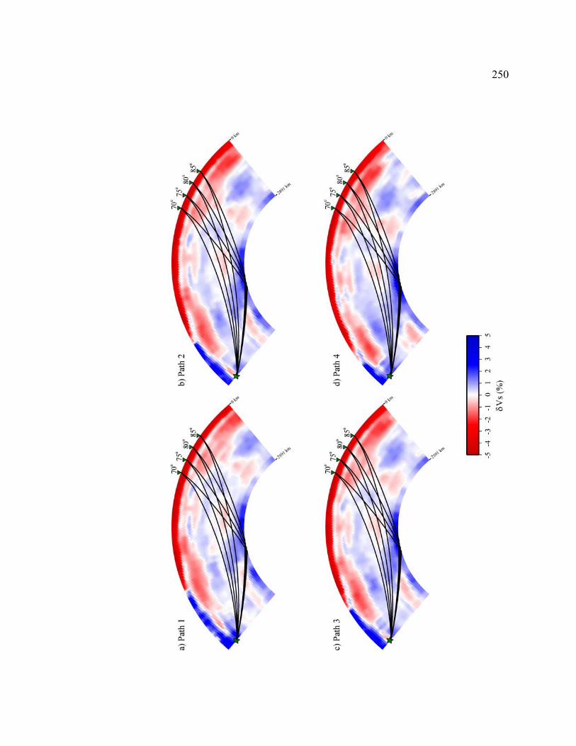
250

251

Supplement 5D Whole mantle cross-sections for model TXBW. Cross-sections for

each of the four Paths we computed synthetic seismograms for are shown. Color scaling

is based on δVS. Ray path geometry is shown for the phases S and ScS for a 500 km deep

event (green star) recorded at receivers (green triangles) with epicentral distances 70º,

75º, 80º, and 85º.

252

253

Supplement 5E Comparison of synthetics computed for the 1-D D" models of Lay et al.

(2004b, drawn in gray) with synthetics created for model LAYB (drawn in black). Each

panel displays synthetics for the labeled Path. Synthetics are aligned and normalized to

unity on the phase S, and calculated for a dominant period of 4 sec.

254

255

Supplement 5F Comparison of synthetics computed for models THOM1.5 (drawn in

gray) and THOM2.0 (drawn in black). Each panel displays synthetics for the labeled

Path. Synthetics are aligned and normalized to unity on the phase S, and calculated for a

dominant period of 5 sec.

APPENDIX A

COMPANION CD

257

A.1 SACLAB

SACLAB is the integration of the standard in solid earth seismic signal

processing, Seismic Analysis Code (SAC), with the standard in technical computing,

MATLAB®, making the computational and programming power of MATLAB® easily

available for use with SAC data files. SACLAB allows one to read SAC data files into

MATLAB® and perform some useful SAC operations in MATLAB®. SACLAB utilities

complement the MATLAB® signal processing toolbox, which has become widely used in

the industry. With SACLAB, programs and data files are portable to any platform that

runs MATLAB® (e.g., Windows, Unix, Linux, etc.). SACLAB foster interdisciplinary

collaboration since MATLAB® can be found in most departments. Also, the extensive

documentation in MATLAB® provides a better understanding of the algorithms used, and

makes it easy to alter a program for a different use.

The Companion CD contains the core SACLAB routines stored in function m-file

format. These routines are located in the saclab directory of the CD. The routines

available on this disc and their primary function are listed below in Table A.1.

258Table A.1 Core SACLAB routines and function. Utility Name Function MATLAB indexing utilities Contents.m SACLAB contents* Reading and writing utilities rsac.m Read SAC binary wsac.m Write SAC binary bsac.m Be SAC – convert MATLAB array to SAC format. Header evaluation utilities lh.m List SAC header ch.m Change SAC header Filtering Utilities bp.m Band pass filter SAC file hp.m High pass filter SAC file lp.m Low pass filter SAC file mavg.m Moving average filter SAC file Misc. Utilities add.m Add constant value to SAC file cut.m Cut SAC file deriv.m Calculate derivatives of SAC file envelope.m Calculate envelope of SAC file integrate.m Integrate SAC file by trapezoidal rule mul.m Multiply SAC file by constant value rmean.m Remove mean of SAC file rtrend.m Remove trend of SAC file taper.m Taper SAC file Plotting Utilities p1.m Plot traces (one trace per subplot) p2.m Plot traces (overlay traces) Function Generation boxfun.m Create boxcar signal kupper.m Create kupper signal refl.m Create reflectivity-like signal ricker.m Create ricker signal triangle.m Create triangle/truncated triangle signal *Uses MATLAB®’s ability to search for available utilities. e.g., if the SACLAB utilities are stored in the directory saclab typing ‘help saclab’ in the MATLAB® command window will retrieve a list of all available SACLAB utilities and their function in a fashion similar to this table.

259

A.2 Animations of seismic wave propagation

In Chapter’s 4 and 5 we introduce the SHaxi method for computation of seismic

wave propagation. One of the nicer features of finite difference simulations is the ability

to produce snapshots of the wave propagation. These snapshots can be processed into

animations of wave propagation. On the companion CD the directory shaxi contains

animations of whole mantle SH-wave propagation. The animations contained are in the

QuickTime format. To view animations in QuickTime format the QuickTime player is

required (http://www.apple.com/quicktime/download/). Because of the large size of the

files best playback performance is obtained by downloading the animations off the CD

onto your hard drive before playing. The animations contained on the CD and the model

parameters for each animation are listed below.

A.2.1 Homogeneous Velocity Models

1. homogeneous_earth_0km.mov Model type: Homogeneous velocity model Vs: 2.0 km/sec Density: 4.0 g/cm3

Source depth: 0 km Dominant period: 30 sec Plot range: -60° ≤ θ ≤ 60° Non-linear Scale: 0.5 Radial grid points: 2,000 Lateral grid points: 10,000

260

2. homogeneous_earth_0km_Vs5.mov

Model type: Homogeneous velocity model Vs: 5.0 km/sec Density: 4.0 g/cm3

Source depth: 0 km Dominant period: 30 sec Plot range: -90° ≤ θ ≤ 90° Non-linear scale: 0.5 Radial grid points: 2,000 Lateral grid points: 10,000

3. homogeneous_earth_500km.mov Model type: Homogeneous velocity model Vs: 2.0 km/sec Density: 4.0 g/cm3

Source depth: 500 km Dominant period: 30 sec Plot range: -60° ≤ θ ≤ 60° Non-linear scale: 0.5 Radial grid points: 2,000 Lateral grid points: 10,000 4. homogeneous_earth_1400km.mov Model type: Homogeneous velocity model Vs: 2.0 km/sec Density: 4.0 g/cm3

Source depth: 1400 km Dominant period: 30 sec Plot range: -60° ≤ θ ≤ 60° Non-linear scale: 0.5 Radial grid points: 2,000 Lateral grid points: 10,000

261

5. LowV_Layer.mov

Model type: Homogeneous velocity model with a low-velocity layer. Model has density 4.0 g/cm3 throughout entire model. Velocity is 3.5 km/sec throughout model except in the low velocity layer. The low velocity layer is contained between the radii 5200 and 5800 km and has a velocity of 2.5 km/sec.

Source depth: 0 km Dominant period: 30 sec Plot range: -70° ≤ θ ≤ 70° Non-linear scale: 0.5 Radial grid points: 2,000 Lateral grid points: 10,000 6. mega_low.mov

Model type: Homogeneous velocity model with an extreme low- velocity layer. Model has density 4.0 g/cm3 throughout entire model. Velocity is 3.5 km/sec throughout model except in the low velocity layer. The low velocity layer has a velocity of 0.5 km/sec.

Source depth: 0 km Dominant period: 30 sec Plot range: -60° ≤ θ ≤ 60° Non-linear scale: 0.5 Radial grid points: 2,000 Lateral grid points: 10,000

262

7. HiV_layer.mov

Model type: Homogeneous velocity model with a high velocity layer. Model has density 4.0 g/cm3 throughout entire model. Velocity is 3.5 km/sec throughout model except in the high velocity layer. The high velocity layer is contained between the radii 5200 and 5800 km and has a velocity of 4.5 km/sec.

Source depth: 0 km Dominant period: 30 sec Plot range: -85° ≤ θ ≤ 85° Non-linear scale: 0.5 Radial grid points: 2,000 Lateral grid points: 10,000 8. Low_Vbody_50km.mov Model type: Homogeneous velocity model with a low-velocity body.

Model has Density 4.0 g/cm3 throughout entire model. Velocity is 3.5 km/sec throughout model except in the low- velocity body which has a S-wave velocity reduction of 5% (Velocity = 3.325 km/sec). The low-velocity body has a radius of 50.0 km, and is centered at a depth of 1371 km, and at an epicentral distance of 30°. A 30 sec dominant period corresponds to a wavelength of 105 km in the homogeneous velocity model. Thus, the size of the low velocity body is on the order of 1-dominant wavelength.

Source depth: 0 km Dominant period: 30 sec Plot range: -10° ≤ θ ≤ 75° Non-linear scale: 0.5 Radial grid points: 2,000 Lateral grid points: 10,000

263

9. Low_Vbody_150km.mov

Model type: Homogeneous velocity model with a low-velocity body. Model has Density 4.0 g/cm3 throughout entire model. Velocity is 3.5 km/sec throughout model except in the low- velocity body. The low-velocity body has a S-wave velocity reduction of 5% (Velocity = 3.325 km/sec) The low-velocity body has a radius of 150.0 km, and is centered at a depth of 1371 km, and at an epicentral distance of 30°. A 30 sec Dominant Period corresponds to a wavelength of 105 km in the homogeneous velocity model. Thus, the size of the low-velocity body is on the order of 3-dominant wavelengths.

Source depth: 0 km Dominant period: 30 sec Plot range: -10° ≤ θ ≤ 75° Non-linear scale: 0.5 Radial grid points: 2,000 Lateral grid points: 10,000

A.2.2 PREM Models

1. prem_500km.mov

Model type: PREM Source depth: 500 km Dominant period: 20 sec Plot range: -180° ≤ θ ≤ 180° Non-linear scale: 0.3 Radial grid points: 2,000 Lateral grid points: 10,000

264

2. prem_500km_12s.mov

Model type: PREM Source depth: 500 km Dominant period: 12 sec Plot range: -10° ≤ θ ≤ 140° Non-linear scale: 0.3 Radial grid points: Never recorded Lateral grid points: Never recorded

3. shinjuku.mov

Model type: PREM Source depth: 500 km Dominant period: 15 sec Plot range: -180° ≤ θ ≤ 180° Non-linear scale: Color scale modified beyond non-linear scaling. Radial grid points: Never recorded Lateral grid points: Never recorded A.2.3 Other Reference Models

1. txbw_500km.mov

Model type: TXBW (Steve Grand 2002 tomography model) Source depth: 500 km Source location: Lat: -27.7°; Lon: 296.7° Receiver location: Lat: 34.0°; Lon: 243.1° Dominant period: 6 sec Plot range: -5° ≤ θ ≤ 90° Non-linear scale: 0.3 Radial grid points: 3,000 Lateral grid points: 30,000 Reference: Grand, S.P., 2002. Mantle shear-wave tomography and the

fate of subducted slabs. Philos. Trans. R. Soc. Lond. Ser. A-Math. Phys. Eng. Sci., 360 (1800), 2475-2491.

265

A.2.4 D" discontinuity models

1. thom2.mov

Model type: PREM w/ D" discontinuity based on Thomas et al. (2004) Source depth: 500 km Dominant period: 10 sec Plot range inset: -5° ≤ θ ≤ 90° Plot range zoom: 25° ≤ θ ≤ 55°; 3480 km ≤ r ≤ 4500 km Non-linear scale: 0.3 Radial grid points: 2,750 Lateral grid points: 20,000 Reference: Thomas, C., Garnero, E.J., & Lay, T., 2004. High-

resolution imaging of lowermost mantle structure under the Cocos plate, Journal of Geophysical Research-Solid Earth, 109 (B8).