DAMAGE IDENTIFICATION, PROGRESSION, AND CONDITION RATING OF

BRIDGE DECKS USING MULTI-MODAL NON-DESTRUCTIVE TESTING

By

BRIAN M. PAILES

A Dissertation submitted to the

Graduate School-New Brunswick

Rutgers, The State University of New Jersey

in partial fulfillment of the requirements

for the degree of

Doctor of Philosophy

Graduate Program in Civil and Environmental Engineering

written under the direction of

Dr. Nenad Gucunski

and approved by

____________________

____________________

____________________

____________________

New Brunswick, New Jersey

May 2014

ii

ABSTRACT OF THE DISSERTATION

Damage Identification, Progression, and Condition Rating of Bridge Decks Using Multi-Modal

Non-Destructive Testing

by BRIAN M. PAILES

Dissertation Director:

Dr. Nenad Gucunski

Bridges are an important part of the nation’s infrastructure and due to the limited budgets

available to keep them properly maintained, the methods of evaluation and damage identification

must improve in accuracy and cost-effectiveness. For the industry of bridge evaluation and

damage identification the research area that provides the greatest potential is multi-modal non-

destructive testing (NDT). A multi-modal NDT approach to condition assessment allows for the

identification of several different deterioration states, in turn providing a more complete condition

assessment. Research was conducted to develop a methodology and program to convert multi-

modal NDT data from bare reinforced concrete bridge decks into a condition-based assessment.

The NDT methods utilized were electrical resistivity (ER), half-cell potential (HCP), ground

penetrating radar (GPR), impact echo (IE), and chain drag (CD). Data for each of these methods

was collected on 12 bridge decks located in various geographic locations. Correlations were

identified between the NDT methods so as to better understand the relationship between the

methods and concrete deterioration. Some of the identified correlations include a strong

association of low cover depth with deterioration, ER and HCP measurements being highly

related, and GPR attenuation associated with locations of deterioration identify by ER, HCP, and

CD. The identified correlations were used to develop a statistics-based approach to threshold

identification for ER, HCP, and GPR. Threshold values are highly relative; therefore, a statistical

approach provides a more effective and robust threshold identification methodology. Using the

iii

identified thresholds, the multi-modal NDT data was fused and converted into a deterioration-

based condition assessment that identifies locations of corrosive environment, active corrosion,

delamination/lateral cracking, and severe delamination. The condition assessment program also

rates the bridge decks using established and federally mandated rating systems created by the

National Bridge Inventory and American Association of State Highway and Transportation

Officials. This research resulted in a more effective multi-modal NDT condition assessment of

bridge decks. Improved multi-modal NDT will provide bridge owners and maintenance

personnel an improved tool to assess bridge decks and to make decisions regarding their

maintenance.

iv

ACKNOWLEDGMENTS

I would like to thank my advisor, Dr. Nenad Gucunski, for providing me with immeasurable

amounts of guidance and support. I would like to also thank my thesis committee members, Dr.

Ali Maher, Dr. Hao Wang, and Dr. Michael Brown.

I would also like to acknowledge the help of Arezoo Imani, Farhad Fetrat, Hooman Parvardeh,

Sabine Krushchwitz, Shane Mott, Chris Mazzotta, Ken Lee, Francisco Romero, Erica Erlanger,

Ronald Guillen, Insung Hwang, Daniel Guillen, Kevin Clark, Michael Morales, Rich Szatkowski,

and Daniel Usher for their help in data collection. I would also like to thank Jeffery Milton, Dave

Meggers, and Jim Leaden for taking time out of their schedules to discuss how departments of

transportation use and apply federally mandated bridge rating systems.

I would also like to thank my parents, Lawrence and Goldie Pailes, who have provided me with

love and support. Without them, I would have never become the person that I am today.

Last, but not least, I would like to thank “The Crew,” Ben, Da, Derek, Kyle, Nils, and Zack.

v

TABLE OF CONTENTS

Abstract of the Dissertation ............................................................................................................. ii

Acknowledgments........................................................................................................................... iv

Table of Contents ............................................................................................................................. v

List of Tables ................................................................................................................................ viii

List of Figures .................................................................................................................................. x

List of Equations ........................................................................................................................... xiv

Symbols and Abbreviations ........................................................................................................... xv

Introduction ...................................................................................................................................... 1

Objectives ........................................................................................................................................ 5

Literature Review............................................................................................................................. 6

Corrosion of Reinforced Concrete ............................................................................................... 6

Electrical Resistivity (ER) ........................................................................................................... 8

Half-Cell Potential ..................................................................................................................... 10

Ground Penetrating Radar .......................................................................................................... 12

Impact Echo ............................................................................................................................... 14

Chain Drag ................................................................................................................................. 16

Non-Destructive Testing Data Fusion........................................................................................ 17

Methods and Materials ................................................................................................................... 21

Non-Destructive Testing Methods ............................................................................................. 21

Equipment Details .................................................................................................................. 23

vi

Data Collection .......................................................................................................................... 25

Data Comparisons ...................................................................................................................... 27

Threshold Analysis .................................................................................................................... 27

Condition Assessment ................................................................................................................ 28

Condition Rating ........................................................................................................................ 30

Presentation of Deck Condition ................................................................................................. 34

Data Agreement Rating.............................................................................................................. 35

Alternate Grid Spacing .............................................................................................................. 40

Non-Destructive Test Method Survey ....................................................................................... 41

Results and Discussion .................................................................................................................. 41

Data Comparisons ...................................................................................................................... 41

Comparisons between Electrical Resistivity and Half-Cell Potential .................................... 41

Ground Penetrating Radar ...................................................................................................... 44

Impact Echo ........................................................................................................................... 47

Cover Depth ........................................................................................................................... 52

Spatial Comparisons .............................................................................................................. 56

Comparisons with Time ......................................................................................................... 59

Threshold Analysis .................................................................................................................... 67

Half-Cell Potential Threshold Analysis ................................................................................. 68

Electrical Resistivity Threshold Analysis .............................................................................. 72

Ground Penetrating Radar Threshold Analysis...................................................................... 74

vii

Application on Other Structures ............................................................................................ 79

Condition Assessment ................................................................................................................ 84

Condition Rating ........................................................................................................................ 88

Data Agreement Rating.............................................................................................................. 90

Multi-Modal Condition Assessment Program ........................................................................... 92

Alternate Grid Spacing .............................................................................................................. 94

Findings ....................................................................................................................................... 105

Conclusions .................................................................................................................................. 106

Recommendations ........................................................................................................................ 108

Future Work ................................................................................................................................. 109

References .................................................................................................................................... 112

Acknowledgement of Previous Publication ................................................................................. 114

Appendices ................................................................................................................................... 115

Appendix 1 – Non-Destructive Test Method Survey ............................................................... 116

Appendix 2 – MATLAB Code for Multi-Modal Condition Assessment ................................ 119

Appendix 3 – Sample Output from Condition Assessment Code ............................................ 158

Appendix 4 –Condition Plots of Evaluated Bridges ................................................................ 161

viii

LIST OF TABLES

Table 1: Interpretation of concrete resistivity (Feliu, Gonzalez and Andrade 1996) ..................... 10

Table 2: Details and descriptions of the structures involved in this research ................................ 26

Table 3: Description and importance of identified damage states ................................................. 29

Table 4: National Bridge Inspection Standards (Ryan, et al. 2006) ............................................... 31

Table 5: AASHTO Bridge Element rating system (AASHTO 2011) ............................................ 31

Table 6: NBIS rating criteria based on multi-modal NDT results ................................................. 33

Table 7: Multi-modal NDT data agreement rating tables .............................................................. 37

Table 8: Situations of complete NDT data agreement ................................................................... 39

Table 9: Agreement and disagreement between IE and CD results ............................................... 48

Table 10: Comparison of severe delamination identification between CD and IE ........................ 49

Table 11: Average NDT measurement based on impact echo signal rating .................................. 50

Table 12: Average cover depth for various condition states .......................................................... 53

Table 13: Average cover depth for impact echo signal ratings ...................................................... 53

Table 14: Spatial agreement in condition between all methods, in percentage ............................. 58

Table 15: Spatial agreement in condition between all methods, in percentage, HCP scaled to

100%, ............................................................................................................................................. 59

Table 16: Change in percentage of agreement from general threshold to individual thresholds ... 59

Table 17: Average resistivity based on changing half-cell potential values (Haymarket, Virginia)

....................................................................................................................................................... 61

Table 18: Comparison of GPR threshold values with average GPR amplitude............................. 79

Table 19: Threshold analysis results .............................................................................................. 80

Table 20: Nonduplicating condition quantities .............................................................................. 86

Table 21: Duplicating damage quantities....................................................................................... 87

Table 22: NBIS rating according to NDT analysis ........................................................................ 89

Table 23: AASHTO condition rating results ................................................................................. 90

ix

Table 24: NDT data agreement rating and percentage of complete agreement ............................. 92

Table 25: Sample input file for the condition assessment program ............................................... 93

Table 26: Percent reduction in amount of test points for various grids ....................................... 105

x

LIST OF FIGURES

Figure 1: Ground penetrating radar survey (Haymarket, Virginia) ................................................. 4

Figure 2: Half-cell potential survey (Haymarket, Virginia)............................................................. 4

Figure 3: Typical corrosion reaction ................................................................................................ 7

Figure 4: Relative size of iron and its oxides (Pilling-Bedworth Ratio) (McCafferty 2010) ........... 8

Figure 5: Four-point Wenner resistivity probe measurement and setup .......................................... 9

Figure 6: Half-cell potential measurement and setup .................................................................... 11

Figure 7: Collection and analysis of ground penetrating radar data .............................................. 13

Figure 8: GPR waveform (A-scan) ................................................................................................ 14

Figure 9: Collection and analysis of impact echo data - after (Gucunski, Slabaugh, et al. 2007) . 16

Figure 10: Progression of bridge deck deterioration and methods of evaluation – after (Gucunski,

Feldmann, et al., Multimodal condition assessment of bridge decks by NDE and its validation

2009) .............................................................................................................................................. 22

Figure 11: Non-destructive testing of a bridge deck, A) electrical resistivity, B) half-cell potential,

C) ground penetrating radar, D) chain drag, E & F) impact echo .................................................. 24

Figure 12: Various data presentation method (Haymarket, Virginia) ............................................ 35

Figure 13: Relative half-cell potential based on resistivity ............................................................ 42

Figure 14: Cumulative frequency distribution of half-cell potentials based on resistivity for all 12

bridges ............................................................................................................................................ 44

Figure 15: Comparison of average relative GPR amplitude to ER ................................................ 45

Figure 16: Comparison of average relative GPR amplitude to HCP ............................................. 46

Figure 17: HCP overlaid with relative GPR amplitude (Haymarket, Virginia) ............................. 47

Figure 18: Cumulative frequency distribution of resistivity based on impact echo signal rating .. 50

Figure 19: Cumulative frequency distribution of half-cell potential based on impact echo signal

rating .............................................................................................................................................. 51

xi

Figure 20: Cumulative frequency distribution of relative GPR amplitude based on impact echo

signal rating .................................................................................................................................... 52

Figure 21: Average cover depth for distribution of half-cell potentials ........................................ 54

Figure 22: Average cover depth for distribution of relative amplitudes ........................................ 55

Figure 23: Average cover depth for distribution of resistivity ....................................................... 56

Figure 24: Areas of the 2009 ER and HCP surveys below 40 kohm·cm and −350 mV CSE

(Haymarket, Virginia) .................................................................................................................... 57

Figure 25: Distribution of half-cell potentials based on electrical resistivity for various years

(Haymarket, Virginia) .................................................................................................................... 60

Figure 26: Areas of ER surveys in 2009 and 2011 below 40 kohm·cm (Haymarket, Virginia) .... 62

Figure 27: Areas of HCP surveys in 2009 and 2011 below −350 mV CSE (Haymarket, Virginia)

....................................................................................................................................................... 63

Figure 28: Areas of GPR surveys in 2009 and 2011 below −20 dB (Haymarket, Virginia) ......... 64

Figure 29: Areas of IE surveys in 2009 and 2011 with a signal rating of 3 or 4 (Haymarket,

Virginia) ......................................................................................................................................... 65

Figure 30: Areas of CD surveys in 2009 and 2011 with a severe delamination (Haymarket,

Virginia) ......................................................................................................................................... 66

Figure 31: Influence of surrounding location’s 2009 condition on the central test location’s 2011

condition (Haymarket, Virginia) .................................................................................................... 67

Figure 32: Cumulative frequency distribution of HCP data filtered according to resistivity

(Haymarket, Virginia) .................................................................................................................... 69

Figure 33: Slope of the cumulative frequency distribution of filtered HCP data (Haymarket,

Virginia) ......................................................................................................................................... 70

Figure 34: Cumulative frequency distribution of ER data filtered according to HCP data

(Haymarket, Virginia) .................................................................................................................... 73

Figure 35: Delta curve of filtered ER cumulative frequency data (Haymarket, Virginia) ............. 74

xii

Figure 36: Cumulative frequency distribution of GPR amplitude filtered by ER and HCP data

(Haymarket, Virginia) .................................................................................................................... 76

Figure 37: Cumulative frequency distribution of GPR amplitude filtered by ER and CD data

(Haymarket, Virginia) .................................................................................................................... 77

Figure 38: Cumulative frequency distribution of GPR amplitude filtered by ER, HCP, and CD

data (Haymarket, Virginia) ............................................................................................................ 77

Figure 39: GPR threshold analysis delta curves (Haymarket, Virginia) ........................................ 78

Figure 40: Slope of the cumulative frequency distribution of filtered HCP data (Sandstone,

Minnesota) ..................................................................................................................................... 81

Figure 41: Slope of the cumulative frequency distribution of HCP data filtered according to

resistivity (Elkton, Maryland) ........................................................................................................ 82

Figure 42: Delta curve of filtered ER cumulative frequency data (Almond, New York) .............. 83

Figure 43: GPR threshold analysis delta curves (Sandstone, Minnisota) ...................................... 83

Figure 44: GPR threshold analysis delta curves (Upper Freehold Township, New Jersey) .......... 84

Figure 45: Condition assessment of Route 15 Bridge in Haymarket Virginia .............................. 85

Figure 46: Input information for the condition assessment code ................................................... 93

Figure 47: Analysis of ER and HCP measured values for changing survey grid spacing ............. 95

Figure 48: Quantities of damage area based on grid spacing......................................................... 96

Figure 49: ER survey results using various grid spacings (Rt. 18 Neptune, New Jersey) ............. 97

Figure 50: HCP survey results using various grid spacings (Rt. 18 Neptune, New Jersey) .......... 98

Figure 51: Percent change in detection area of electrical methods for various square grid spacings

....................................................................................................................................................... 99

Figure 52: Percent change in detection area of electrical methods for various rectangular grid

spacings ........................................................................................................................................ 100

Figure 53: Percent change in detection area of acoustic methods for various square grid spacings

..................................................................................................................................................... 101

xiii

Figure 54: Percent change in detection area of acoustic methods for various rectangular grid

spacings ........................................................................................................................................ 101

Figure 55: Percent change in average measurements due to various grid spacings ..................... 102

Figure 56: ER survey results using various grid spacings (Haymarket, Virginia) ....................... 103

Figure 57: HCP survey results using various grid spacings (Haymarket, Virginia) .................... 104

Figure 58: Condition assessment of I-495 South Bridge in Wilmington, Delaware .................... 162

Figure 59: Condition assessment of I-195 East Bridge in Upper Freehold, New Jersey ............. 162

Figure 60: Condition assessment of Pequea Boulevard Bridge in Conestoga, Pennsylvania ...... 163

Figure 61: Condition assessment of School House Road Bridge in Middletown, Pennsylvania . 163

Figure 62: Condition assessment of Route 123 Bridge in Sandstone, Minnesota ....................... 164

Figure 63: Condition assessment of Route 15 Bridge in Haymarket, Virginia ........................... 164

Figure 64: Condition assessment of Route 18 Bridge in Neptune, New Jersey........................... 165

Figure 65: Condition assessment of Route 21 Bridge in Almond, New York ............................. 165

Figure 66: Condition assessment of Route 273 Bridge in Elkton, Maryland .............................. 166

Figure 67: Condition assessment of Route 47 Bridge in Deptford Township, New Jersey ......... 166

Figure 68: Condition assessment of Route 93 Bridge in Sumner, Iowa ...................................... 167

Figure 69: Condition assessment of West Bangs Ave Bridge in Neptune, New Jersey .............. 167

xiv

LIST OF EQUATIONS

Resistivity equation .......................................................................................................................... 9

Variance-covariance equation ........................................................................................................ 19

Correlation equation....................................................................................................................... 19

Centered finite difference formula ................................................................................................. 71

xv

SYMBOLS AND ABBREVIATIONS

a ........................ Resistivity probe spacing

AASHTO ......... American Association of State Highway and Transportation Officials

BAM ................ Germany’s Federal Institute for Materials Research and Testing

CD .................... Chain drag

CSE .................. Copper sulfate electrode

DOT ................. Department of transportation

ER .................... Electrical resistivity

FHWA .............. Federal Highway Administration

GPR .................. Ground penetrating radar

HCP .................. Half-cell potential

HSCP ............... Human Subjects Certification Program

I ........................ Electrical current, amperes

IE ...................... Impact echo

IRB ................... Institutional Review Board

KDOT .............. Kansas Department of Transportation

LTBP ................ Long Term Bridge Performance

NBIS ................ National Bridge Inspection Standards

xvi

NDT ................. Non-destructive testing

NJDOT ............. New Jersey Department of Transportation

ρ ....................... Resistivity, ohm·cm

R ....................... Resistance, ohm

UE .................... Ultrasonic echo

USW................. Ultrasonic Surface Wave

V....................... Voltage, v

VDOT .............. Virginia Department of Transportation

1

INTRODUCTION

Bridges are an important part of the nation’s infrastructure and due to the limited budgets

available to keep them properly maintained, the methods of evaluation and damage identification

must improve in accuracy and cost-effectiveness. At the forefront of bridge evaluation and

damage identification is non-destructive testing (NDT). NDT is an effective form of condition

assessment that continues to advance through increases in accuracy while time requirements and

costs decrease. There are many different NDT methods capable of evaluating and identifying

different types of damage in reinforced concrete structures. These NDT methods include, but are

not limited to, ground penetrating radar (GPR), impact echo (IE), half-cell potential (HCP),

electrical resistivity (ER), surface wave testing, ultrasonic wave testing, infrared thermography,

and many others. Each of these methods uses a unique physical principal of the bridge materials

to identify locations of deterioration. For example, HCP is able to identify active corrosion by

measuring the electrical potential difference between the steel reinforcement and a reference

electrode. IE locates delaminations by impacting the concrete surface and evaluating the

frequency of the reflecting waves. Unfortunately, there is no single NDT technology that is

capable of identifying all of the various deterioration phenomena that can affect a bridge deck.

To get a complete understanding of a bridge deck’s condition, NDT practitioners have started

surveying bridge decks using a multi-modal NDT approach. Using a multi-modal NDT approach

allows for the identification of several different damage states, resulting in a more complete

understanding of a deck’s condition.

While a multi-modal NDT approach provides a more complete understanding of a bridge deck’s

condition, this approach also creates several difficulties. The practitioner must deal with

significantly more data, understand how to properly fuse that data, and interpret the data fusion.

It is the aim of this research to develop methodologies and protocols for the data analysis and

2

presentation of multi-modal NDT data so that it provides a more complete condition assessment

of a bridge deck.

There are four primary gaps in the practice of multi-modal NDT that this research is aimed at

addressing;

1. Results of NDT testing are commonly provided to bridge owners and maintenance

personnel in the form of contour plots based on the NDT measurement scale.

Current practice when providing a bridge owner with NDT results is to provide those results in

the form of a contour plot. The contour scale is based on the units and measurement range of the

NDT device, in which colors are used to indicate the areas of deterioration and sound concrete.

Figure 1 is the result of a GPR survey on a bridge deck in Haymarket, Virginia. The contour

scale is in decibels of signal attenuation. Most bridge owners and maintenance personnel are not

familiar with GPR nor signal attenuation, therefore, this scale has no tangible meaning to them.

The only way for them to identify areas of damage would be through reading any supplemental

report accompanying the figure and referencing the color scheme. It is typical to assume that

warm colors, red and yellow, indicate damage and cool colors, blues and greens, indicate sound

concrete. However, what kind of damage do these warm colors indicate? What is the difference

in damage between red and yellow? A plot like Figure 1 creates more questions than answers for

a person without an NDT background. NDT Results based on the scale of the measurement

device is not the most effective way of presenting NDT results to people responsible for bridge

maintenance and operation. These results do not provide a bridge owner or maintenance

personnel with information that they can directly use in decision-making.

3

2. When multiple NDT methods are performed on a structure, results of each method are

typically presented separately. True data fusion between the multiple methods is not

being conducted.

A GPR survey of a reinforced concrete bridge deck alone is not enough information to accurately

identify every deterioration state. Therefore, a multi-modal NDT approach is taken to provide a

more complete condition assessment. The current practice when conducting a multi-model NDT

survey is to provide each method’s results in an individual plot. Besides some qualitative

assessment typically provided in an accompanying report, there is no true data fusion between the

NDT methods, nor is there a quantitative analysis. Each NDT method measures a different

parameter in the deck; therefore, they can sometimes give differing results, which if presented in

different plots to a person untrained in NDT will indicate conflicting results. Figure 1 and Figure

2 are the results of GPR and HCP surveys conducted on the same bridge deck in Haymarket,

Virginia. These two methods measure completely different parameters in the bridge deck;

therefore, the areas of agreement and disagreement between the warm colors do not necessarily

indicate the accuracy of the surveys. To someone untrained in NDT, they could interpret areas of

disagreement as incorrect or conflicting results. In actuality, that is not the case because each

method is identifying different condition states. The true condition of the bridge can only be

identified through the fusion of these two survey results.

4

Figure 1: Ground penetrating radar survey (Haymarket, Virginia)

Figure 2: Half-cell potential survey (Haymarket, Virginia)

3. Multi-modal NDT results are not commonly being used to understand how damage will

progress in the future.

With the application of multi-modal NDT and periodic monitoring of individual structures, more

research needs to be focused at understanding where damage will spread and how fast. Each

NDT method describes a different aspect of reinforced concrete degradation. By understanding

what methods detect which stage of deterioration and how these stages progress, a better

understanding of bridge deterioration will be gained. For instance ER detects a corrosive

environment, while HCP measures potential to identify if corrosion is active. Areas identified in

5

the ER survey as corrosive environment, which are passive in the HCP survey, could indicate that

these locations corrosion will activate in the near future. Associations like this could lead to more

accurate predictions regarding the future condition of a bridge.

4. Overall, NDT as a decision-making tool for bridge owners and maintenance operations is

limited because of several gaps in the multi-modal NDT practice.

Solutions to the first three gaps in the NDT practice will make NDT a more efficient and effective

decision-making tool for bridge owners and maintenance personnel. The reason that NDT

condition surveys are performed on structures is to identify deterioration processes and locate

damage, so that bridge owners can make decisions regarding maintenance. The goal of NDT

practitioners should be to direct NDT methods towards what bridge owners and maintenance

operations need.

OBJECTIVES

The four primary problems with the current NDT practice were outlined in the Introduction. To

solve these problems, several research objectives were established. The primary research

objective is to develop an automated condition assessment program that will take post-processed

NDT data and convert it into a damage-based condition assessment.

This primary objective is a large and very broad goal. In order to complete this primary

objective, there are several secondary objectives that will need to be accomplished, as follow:

• Identify trends and correlations in the multi-modal NDT data.

• Develop a statistics-based approach to threshold identification.

• Convert NDT data into a condition-based assessment.

• Convert the multi-modal NDT condition assessment into a rating using already

established and federally mandated rating systems.

6

• Present the condition of the deck in an accurate and genuine way.

• Identify the strength of agreement in damage identification between the NDT methods.

• Validate the current sampling procedures and identify if larger NDT sampling can be

used to more quickly establish general deck condition.

• Drive NDT surveys and results to be focused more on meeting the needs of bridge

owners and maintenance operations.

LITERATURE REVIEW

As a part of this research, an in-depth literature review was conducted on the corrosion process of

reinforced concrete, the different NDT methods being implemented, and the fusion of multi-

modal NDT data. The focus of this research is NDT to identify concrete deterioration caused by

chloride-induced corrosion. Chloride-induced corrosion is not the only deterioration mechanism

that affects reinforced concrete decks; it is, however, the most common (ACI Committee 222

2001). Other deterioration mechanisms that can occur in reinforced concrete bridge decks

include, but are not limited to, carbonation, alkali-silica reaction, freeze-thaw, and mechanical

distress (Ryan, et al. 2006).

CORROSION OF REINFORCED CONCRETE

Corrosion is an electrochemical reaction involving iron, water, and oxygen. In the presence of

water and oxygen, iron will release two electrons and combine with oxygen and hydrogen to

create ferric oxide at the anodic region of the corrosion reaction (Figure 3). At the cathodic

region of the reaction, the free electrons will combine with oxygen and water to create hydroxide.

Iron will only release its electrons if there are elements willing to accept the freed electrons,

resulting in a balanced reaction. Concrete normally provides a highly alkaline environment, with

pH of approximately 13.5 (Rapa and Hartt 1999), in which steel is naturally passive (Broomfield

7

2007). The passivity of steel in a highly alkaline environment is due to the formation of a

protective oxide film (Funahashi 1990). The protective oxide film is formed along the surface of

the steel and protects the steel from more severe corrosion (Funahashi 1990). However, chloride

or carbon dioxide, which can diffuse into the concrete matrix from the external environment, can

lower a concrete’s pH and depassivate the steel (Poulsen and Mejlbro 2006). Corrosion of

concrete reinforcement creates a progression of damage, starting with section loss, formation of

iron oxide, concrete cracking, delamination, and eventual spalling. The concrete damage that

results from corrosion activity is due to the accumulation of ferric oxide beneath the concrete

surface. Ferric oxide molecules are larger than the original iron (Figure 4); therefore, as they

form, there is an increase in material volume at the steel level. This increase in volume creates

expansive forces inside the concrete that result in the formation of concrete tensile stresses.

Concrete, which is relatively weak in tension, will eventually crack due to these stresses and lead

to delamination and an eventual spall.

Figure 3: Typical corrosion reaction

8

Figure 4: Relative size of iron and its oxides (Pilling-Bedworth Ratio) (McCafferty 2010)

The deterioration process of reinforced concrete can be identified and monitored through the use

of many different NDT methods. The NDT methods used to identify the condition of bridge

decks for this research are; ER, HCP, GPR, IE, and chain drag (CD). These methods were

specifically selected due to their combined ability to capture the full spectrum of concrete

deterioration with regard to corrosion activity.

ELECTRICAL RESISTIVITY (ER)

Electrical resistivity is an NDT method that measures the concrete’s ability to pass electrical

current. Concrete’s ability to support current flow is an important factor in deterioration, because

corrosion is an electrochemical reaction requiring current flow. If the concrete is highly resistive,

then that limits the ability of ions to move between the cathodic and anodic regions of the

corrosion reaction. If the concrete has a low resistivity, then the corrosion reaction will have no

difficulty in passing current, allowing for the corrosion reaction to occur quite rapidly and over a

larger area. The resistivity of concrete is highly dependent on the concrete’s moisture content,

permeability, chloride content, and temperature (Elkey and Sellevold 1995). The ability of the

concrete to pass current increases as water and free ions accumulate in the concrete matrix and

0 1 2 3 4 5 6 7

Relative Size

Fe

FeO

Fe3O

4

Fe(OH)2

Fe(OH)3∙3H

2O

9

the concrete pores increase in size and continuity. The corrosion reaction is highly dependent on

the presence of water, chlorides, and current flow; therefore, areas in which the resistivity is low

indicate an environment that is conducive to corrosion activity. There are several methods to

measure concrete resistivity; however, the most common method in civil engineering applications

is the four-point Wenner method (Kessler, et al. 2008). The four-point Wenner method involves

passing of current between two exterior probes and measuring the potential between two

intermediate probes, all spaced at equal intervals, a (Figure 5). Equation (1) is used to calculate

resistivity (ρ, kohm·cm) using the parameters measured by the Wenner method; current (I,

amperes), potential (V, volts), resistance (R, kohm), and probe spacing (a, inches).

Figure 5: Four-point Wenner resistivity probe measurement and setup

� =

2���

� (1)

10

In the literature, there have been several interpretations of resistivity measurements made on

reinforced concrete. Table 1 provides a general interpretation of resistivity values with respect to

risk of corrosion. Most studies agree that a concrete resistivity less than 10 kohm·cm is

associated with a very high risk of steel corrosion activity (Elkey and Sellevold 1995) (Malhotra

and Carino 2004) (Feliu, Gonzalez and Andrade 1996). However, there has been much variation

and debate in identifying at what resistivity value the risk of corrosion is low. Resistivity values

above which risk of corrosion is low have been given as 10 kohm·cm (Elkey and Sellevold 1995),

20 kohm·cm (Bungey 1989), 30 kohm·cm (Morris, et al. 2002), and 50 kohm·cm (Feliu, Gonzalez

and Andrade 1996).

Table 1: Interpretation of concrete resistivity (Feliu, Gonzalez and Andrade 1996)

Concrete Resistivity (kohm·cm) Risk of Corrosion

< 10 High

10 – 50 Moderate

50 – 100 Low

> 100 Negligible

HALF-CELL POTENTIAL

Half-cell potential is an NDT method capable of identifying locations of active corrosion in reinforced

concrete. HCP measurements are conducted by electrically connecting a reference electrode to the steel

reinforcement and measuring the potential difference between them (

11

Figure 6). In most civil engineering applications, the reference electrode is a copper/copper

sulfate electrode (CSE) (ACI Committee 222 2001), comprised of a copper rod inside a saturated

solution of copper sulfate. HCP measurements are a probabilistic measurement, in that they

indicate the probability of active corrosion. ASTM C876-09, the Standard Test Method for

Corrosion Potentials of Uncoated Reinforcing Steel in Concrete (ASTM 2009) indicates that

when the HCP is less than −350 mV CSE, the probability of active corrosion is 90%. When the

potential is greater than −200 mV CSE, there is a 90% probability of a passive condition, and

between those ranges corrosion activity is uncertain. The threshold values provided by ASTM

C876-09 are not absolute and are not applicable in every situation (Elsener, et al. 2003). HCP

threshold values can shift depending on several factors. These factors include concrete

temperature, moisture and oxygen content, resistivity, presence of ions, surface treatments, stray

currents, and corrosion-inhibiting admixtures (Gu and Beaudoin 1998). The concrete’s

concentration of moisture and oxygen has a significant effect on potential measurements. An

increase in moisture content will cause a negative shift in potential and a decrease in oxygen

content will also cause a negative shift in the potential (Gu and Beaudoin 1998).

Figure 6: Half-cell potential measurement and setup

12

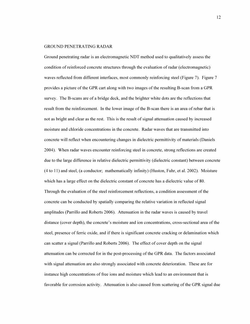
GROUND PENETRATING RADAR

Ground penetrating radar is an electromagnetic NDT method used to qualitatively assess the

condition of reinforced concrete structures through the evaluation of radar (electromagnetic)

waves reflected from different interfaces, most commonly reinforcing steel (Figure 7). Figure 7

provides a picture of the GPR cart along with two images of the resulting B-scan from a GPR

survey. The B-scans are of a bridge deck, and the brighter white dots are the reflections that

result from the reinforcement. In the lower image of the B-scan there is an area of rebar that is

not as bright and clear as the rest. This is the result of signal attenuation caused by increased

moisture and chloride concentrations in the concrete. Radar waves that are transmitted into

concrete will reflect when encountering changes in dielectric permittivity of materials (Daniels

2004). When radar waves encounter reinforcing steel in concrete, strong reflections are created

due to the large difference in relative dielectric permittivity (dielectric constant) between concrete

(4 to 11) and steel, (a conductor; mathematically infinity) (Huston, Fuhr, et al. 2002). Moisture

which has a large effect on the dielectric constant of concrete has a dielectric value of 80.

Through the evaluation of the steel reinforcement reflections, a condition assessment of the

concrete can be conducted by spatially comparing the relative variation in reflected signal

amplitudes (Parrillo and Roberts 2006). Attenuation in the radar waves is caused by travel

distance (cover depth), the concrete’s moisture and ion concentrations, cross-sectional area of the

steel, presence of ferric oxide, and if there is significant concrete cracking or delamination which

can scatter a signal (Parrillo and Roberts 2006). The effect of cover depth on the signal

attenuation can be corrected for in the post-processing of the GPR data. The factors associated

with signal attenuation are also strongly associated with concrete deterioration. These are for

instance high concentrations of free ions and moisture which lead to an environment that is

favorable for corrosion activity. Attenuation is also caused from scattering of the GPR signal due

13

to large amount of cracking and delamination. The steel cross-section also influences the

magnitude of the GPR reflections. If the steel cross-section is compromised by corrosion then

that along with the formation of large amounts of ferric oxide can decrease the magnitude of the

reflection. This allows for the GPR amplitude evaluation to provide insight into the condition

state of a bridge deck.

Figure 7: Collection and analysis of ground penetrating radar data

Figure 8 provides a GPR waveform; also known as the A-scan. A GPR survey collects A-scans

at the defined sampling increments. These A-scans are then combined to form a B-scan. The B-

scan colors are the result of a gray scale being applied to the distribution of amplitudes. In order

to analyze the GPR data it must go through several processing steps so that the amplitude of the

wave at the concrete/rebar interface can be determined. These corrections include background

removal, time-zero correction, migration, and depth correction. Time-zero correction accounts

for the small bit of air the GPR wave must travel through before it reaches the concrete surface.

Migration corrects the GPR waveforms from the error caused by the motion of the antenna. In

Figure 7 the rebar reflections look like parabolas; which is the result of the antenna’s motion

14

during data collection. Once the GPR data has been corrected, the software tries to identify the

peaks in the data caused by the rebar reflections. The user must then verify all of the software’s

selections since the program will miss peaks and make incorrect selections. The automated

picking is used as an initial pass. Once the proper peaks have been selected then the amplitude at

those locations along with distance measurements are imported into a spreadsheet for analysis.

Figure 8: GPR waveform (A-scan)

IMPACT ECHO

Impact echo is an acoustic NDT method used to identify lateral cracks and delaminations beneath

the concrete surface. IE identifies damage by mechanically striking the concrete surface and

recording the resulting response of the deck. Typically the mechanical impact is caused by

striking a steel bearing or solenoid on the surface of the concrete (Ryan, et al. 2006). The impact

creates stress waves that reflect off of the bottom of the deck and/or intermediate damage

interface (Gucunski, Slabaugh, et al. 2007). A recording device, like a piezoelectric transducer or

accelerometer, is coupled to the surface of the concrete and records the velocity or acceleration of

the response. The recorded signal is captured in the time-domain and converted into the

frequency-domain using the fast Fourier transform. The frequency-domain identifies the energy

levels for the spectrum of frequencies recorded. If the stress wave is reflecting off of the bottom

of a sound deck, then the wave energy will be at a frequency relating to the thickness of the deck

(Figure 9) (Gucunski, Slabaugh, et al. 2007). If there are intermediate reflectors in the deck, like

delaminations or lateral cracks, then there could be secondary peaks in the frequency spectrum or

15

the primary peak could be shifted to a frequency associate with the impeding intermediate

interface (Gucunski, Slabaugh, et al. 2007). This depends if the damage is completely or partially

reflecting the wave energy. If there is a partial reflection, then there will be a primary peak at the

frequency corresponding to the full deck thickness, and a peak corresponding to the intermediate

damage (Gucunski, Slabaugh, et al. 2007). If the damage is so significant that it reflects all of the

wave energy, then the primary peak will be shifted, higher for a delamination, and lower for large

near surface delamination (Gucunski, Slabaugh, et al. 2007). The lower frequency caused by a

large near surface delaminations is a result of the IE device recording the movement of the

delamination when it is impacted. The delamination acts like a beam in flexure as opposed to a

slab.

In the analysis of IE data a numerical value is assigned to each of the conditions identified in

Figure 9. A signal rating of 1 indicates “good condition,” signal rating of 2 indicates “fair

condition,” signal rating of 3 indicates “poor condition,” and a signal rating of 4 indicates

“serious condition.”

16

Figure 9: Collection and analysis of impact echo data - after (Gucunski, Slabaugh, et al. 2007)

CHAIN DRAG

Chain drag is an NDT method that is less sophisticated than the previous NDT methods; however,

it is highly effective at identifying large near-surface delaminations (ASTM 1992). CD uses large

steel chains that are dragged along the surface of a bridge deck to identify large late-stage

delaminations. The CD operator listens to the sound that is created by the chain and when the

pitch of the sound changes to a hollow sound, which is usually of lower pitch than that of the

17

chains on sound concrete; this identifies the location of a delamination (ASTM 1992). In general,

the lower the pitch, the larger the delamination, as with a drum head. When the chains are

dragged over a large late-stage delamination, the flexural vibrations of the delamination cause the

change in sound frequency (ASTM 1992). When the chains are dragged over a section that is not

delaminated, they create a clear ringing sound caused by the chain itself (ASTM 1992). ASTM

D4580, the Standard Practice for Measuring Delaminations in Concrete Bridge Decks by

Sounding covers the operations and specifications to conduct a CD survey (ASTM 1992). The

reason that CD can only find large late-stage delaminations is that the test is dependent on human

hearing. Only large late-stage delaminations create a sound in the audible frequency range,

typically 1 to 4 kHz (Gucunski, Imani, et al. 2013). Therefore, the operators’ skill in detecting a

delamination using CD is highly dependent on their hearing ability and the surrounding ambient

noise level (Henderson, Dion and Costley 1999).

NON-DESTRUCTIVE TESTING DATA FUSION

It is critical to this research to understand each NDT method, how it operates, and how to

properly fuse the results from these different methods together. Horn (Horn 2006) presents an

overview of NDT reliability with regard to the combination of multiple NDT methods. The focus

of the work was on eddy current and ultrasonic testing in the aerospace industry, but the

overarching ideas of the paper are very applicable to data fusion of any technologies in any field.

Horn describes the difference between repeat measurements and using multiple methods to

evaluate a sample. Performing repeat measurements increases the “statistical precision” of the

results, while the use of multiple techniques can allow for each method to reveal phenomena that

the other methods many not be able to detect (Horn 2006). This is a very important statement and

the reason why the use of multi-modal NDT methods is important. The use of several different

methods allows for the detection of different damage states or conditions that would not be

18

identified if only one method was used. Multi-modal NDT provides a more complete assessment

of the test subject.

Research by Horn (Horn 2006) and Gros et al. (Gros, Bousigue and Takahashi 1999) discussed

different ways to fuse the results of two different NDT methods conducted on the same

material/structure. The objective of their work was to combine the results of multiple NDT

methods so that detection errors, like unidentified damage and false damage identification, were

minimized. The methods of fusion included, logical operators “and” and “or”, summation,

maximum amplitude, averaging, weighted averaging, Bayes’ theorem, and Dempster-Shafer

theory (Horn 2006) (Gros, Bousigue and Takahashi 1999). An important step in both Horn (Horn

2006) and Gros’s (Gros, Bousigue and Takahashi 1999) work is that when they were fusing the

NDT results, the data was in the same scale. In Horn’s work, the two different NDT methods

provided results in the same data format, wave amplitude, and Gros’s work used the image pixels

that resulted from the data processing. In both situations, the data being fused had the same scale.

If the data did not have the same scale, the fusion of the data would not produce meaningful

information.

Work done by Huston et al. in 2010 (Huston, Cui, et al. 2010) investigated combining the results

of HCP, GPR, IE, and CD to better understand the condition of a bridge deck in Virginia. Huston

et al. took a purely statistical approach to the fusion of the four NDT results. In order to fuse the

data together, they linearly normalized the results of each method to a 0-1 scale so that each

method had the same scale. Huston et al. plotted the linearized results, which resulted in 660,000

pixels, representing the deck surface. The pixel values were then used to make comparisons

between the different methods. Huston et al. also used pixel blocks as another way to compare

the NDT results. The blocks were taken as 50 x 50 pixel segments and assigned the average

value of the pixels contained in each segment. Huston et al. created a variance-covariance matrix

(Equation (2)) to compare each data point, pixel, and block value of all four test methods. The

19

magnitude of σij indicates the degree to which methods i and j are related to each other. A

negative value of σij indicates that as the value of i increases, the value of j decreases, and a

positive value indicates that as i increases, j also increases.

��� =

1

� − 2����� − �̅������ − �̅��

���

(2)

Along with variance-covariance, Huston et al. also created a correlation matrix (Equation (3)),

which is similar to the covariance analysis in that it assesses if the i and j variable are related.

Huston et al. reported that the statistical correlation of the NDT methods was “relatively weak.”

�� =���

��������/� (3)

Huston et al. also produced several plots of the combined data in order to understand visually

observed correlations and agreement in the data. By taking a mean value of condition estimates

for each method and plotting on a grey scale, black indicated agreement between the methods in

detection of damage and white indicated agreement between the methods in identification of no

damage. The plots indicated that there was better agreement in identifying damage than

agreement in identifying no damage. There were many areas where all of the methods indicated

damage; however, there was a limited area in which all the methods agreed there was no damage.

There was also a significant amount of area that indicated no agreement between the methods

about the condition state.

Huston et al. concluded that the agreement in condition of the four methods was not strong.

However, they state that the combination of several different NDT methods could allow for a

better assessment of bridge deck condition. The conclusion that the four different NDT methods

20

do not have strong correlation is not surprising, since each method is identifying a different

condition, deterioration process, or damage type. This work by Huston et al. shows the

importance of understanding how each NDT method is related and unrelated. Huston et al. were

trying to combine the data without evaluating if these methods have strong correlations based on

their physical principals of operation. For instance, it is expected that HCP and CD have poor

statistical correlation, since HCP is identifying active corrosion and CD identifies large near-

surface delaminations. The statistical correlation of these results is going to be weak, since active

corrosion is an early stage condition compared to delaminations, which are late-stage.

Additionally, delaminations can result from several different deterioration processes, not just

corrosion.

Germany’s Federal Institute for Materials Research and Testing (BAM) conducted multi-modal

NDT research using GPR and ultrasonic echo (UE) in the evaluation of a reinforced concrete slab

and a concrete box girder bridge (Maierhofer, et al. 2008) (Kohl and Streicher 2006). The results

of the work showed that GPR and UE complemented each other due to the differences in

investigation depth and reinforcement detection. GPR signals have difficulty penetrating past

dense reinforcing grids, however, are excellent at evaluating the condition of the first layer of

concrete reinforcement. This makes the investigation of anything past the top layer of

reinforcement difficult for GPR. UE is able to evaluate the concrete cross-section; however, UE

is unable to differentiate between the concrete and steel reinforcement. Through the combination

of GPR and UE data sets, a complete evaluation of the reinforced concrete specimens was

obtained. This work demonstrates how two complementary NDT methods can produce excellent

results when the data is properly merged.

A review was also conducted of work done at Rutgers University regarding the use of multi-

model NDT to evaluate bridge decks (Gucunski, Feldmann, et al. 2010), (Gucunski, Feldmann, et

al. 2009), (Gucunski, Imani, et al. 2013), (Gucunski, Romero, et al. 2010). The deck surveys

21

were conducted using a wide array of NDT methods: ER, HCP, GPR, ultrasonic surface wave

(USW), IE, and CD. The research provides evidence for the benefits of using multiple NDT

methods to evaluate a bridge deck. The different methods provide a complete evaluation of the

bridge deck by identifying damage at varying stages of deterioration. The work also indicated

that each of the different NDT methods indicated similar areas of damage, which improved the

confidence in the overall results. The following is a sampling of the results from these papers;

areas of high GPR attenuation are also associated with HCP indicating active corrosion

(Gucunski, Feldmann, et al. 2010); a deck with no areas of corrosive environment indicated no

areas of active corrosion (Gucunski, Romero, et al. 2010); areas of high GPR attenuation were

verified as damage through coring (Gucunski, Feldmann, et al. 2009); and IE was able to more

completely identify delaminations when compared to CD (Gucunski, Romero, et al. 2010). This

work demonstrates that a more complete evaluation of a bridge deck can be done by using a

multi-modal NDT approach. One overarching step that was missing from this work, however,

was that there was no true fusion of the NDT results. Each NDT result was presented in a

separate plot and none of the results were combined to improve the overall bridge assessment.

All the comparative analyses were done qualitatively, based on a visual assessment of the plots.

METHODS AND MATERIALS

NON-DESTRUCTIVE TESTING METHODS

The five NDT methods used to survey and assess the condition of the bridge decks for this

research are ER, HCP, GPR, IE, and CD. ER and HCP are electrical methods that are capable of

identifying a corrosive environment in concrete and the probability of active corrosion,

respectively. GPR is an electromagnetic method that is able to identify, mostly in qualitative

terms, various types of concrete degradation, which include corrosion, high moisture and chloride

contents, significant cracking and delaminations to a limited degree. IE and CD are acoustic

22

methods that are capable of identifying delaminations and lateral cracking in varying degrees.

These NDT methods were selected because each method is capable of identifying a different

damage state in the progression of concrete deterioration. Figure 10 depicts the progression of

reinforced concrete deterioration as a result of chloride-induced corrosion. Initially, there is the

infiltration of moisture and chlorides into the concrete matrix, then the initiation of corrosion,

then cracking, and eventual delamination, which leads to spalling. At each stage along this

progression, there is a different NDT technology that is best suited to identifying that condition

state. Assessing the condition of a deck simultaneously with these NDT methods provides a more

complete assessment of the deck’s condition, since each stage of the deterioration process can be

identified. There is also some overlap of the technologies, like ER and GPR, which provide the

ability to verify results between different technologies.

Figure 10: Progression of bridge deck deterioration and methods of evaluation – after (Gucunski,

Feldmann, et al. 2009)

23

Equipment Details

The ER surveys (Figure 11-A) were conducted using a four-point Wenner probe connected to a

data logger. The ER electrode spacing was set at 1.5 in. Water was applied to the concrete

surface prior to ER testing to improve the electrical couple between the probes and concrete

surface. The surface layer of a concrete deck is typically drier than the deck thickness as a whole.

This is due to surface moisture evaporation caused by exposure to the sun and wind. Wetting the

deck surface prior to testing helps to remove this dry layer and improve coupling between the

electrode and concrete.

The HCP measurements were collected (Figure 11-B) using a copper/copper sulfate reference

electrode connected to a data logger. Data collection with HCP was done in accordance to

ASTM C876-09. Each bridge deck’s reinforcing steel was verified to be electrically continuous

prior to data collection. Water was applied to the concrete surface prior to HCP testing to aid in

creating an electrical couple between the reference electrode and the concrete.

24

Figure 11: Non-destructive testing of a bridge deck, A) electrical resistivity, B) half-cell potential, C)

ground penetrating radar, D) chain drag, E & F) impact echo

The GPR survey was conducted using a ground-coupled 1.5 GHz antenna collecting at 60 scans

per foot. The antenna was attached to a push cart that was used to scan the surface of the bridge

deck in lines that were perpendicular to the direction of the top layer of reinforcing steel (Figure

11-C). The top layer of steel was in the transverse direction (relative to traffic flow and the

length of the spans) for all of the bridges in this research. Therefore, the GPR survey lines were

conducted in the longitudinal direction.

The IE survey was conducted using an automated IE device called Stepper (Figure 11-E & F).

The device has an array of three IE probes that autonomously progressed across the deck to

collect IE data. The impact source was a steel ball bearing and the recording device was a

piezoelectric transducer. The IE data was analyzed and converted into a numerical scale, 1

25

through 4, according to the analysis outlined in Figure 9. A result of good was rated as 1, fair-2,

poor-3, and serious-4.

The CD survey was conducted using 4 steel chains connected to a steel pipe (Figure 11-D).

These chains were dragged over the surface of the deck to identify locations of delaminations. In

conjunction with the CD survey, hammer sounding was done to delineate the extent of each

delamination that was identified in the CD survey. Data collection with CD was done in

accordance to ASTM D4580.

DATA COLLECTION

The data for this research was collected on twelve bridge decks throughout the United States of

America. It is not the aim of this dissertation to discuss the details of each bridge, since they are

all unique, having different dimensions, load bearing systems, exposure environments, and

geographic locations. While each bridge is unique, they are all similar in that they all have bare

reinforced concrete decks with electrically continuous steel reinforcement. Table 2 provides a

brief overview of the structures that were surveyed as a part of this research. All of these

structures, except the structure in Iowa, are a part of the Long Term Bridge Performance (LTBP)

Program funded by the Federal Highway Administration (FHWA).

26

Table 2: Details and descriptions of the structures involved in this research

Carries Crossing Location Bridge Type Number

of Spans

Deck

Area (ft2)

I-495 South Route 13 Wilmington,

DE Continuous Steel Girder 2 13,716

I-195 East Sharon

Station Rd.

Upper

Freehold

Township, NJ

Simply Supported Steel

Girder 1 3,420

Pequea

Boulevard

Pequea

Creek

Conestoga,

PA

Simply Supported

Prestressed Concrete Girder 2 6,952

School

House Road

State Route

283

Middletown,

PA Continuous Steel Girder 2 10,296

State Route

123 Kettle River

Sandstone,

MN Deck Truss 4 6,400*

State Route

15 Interstate 66

Haymarket,

VA Continuous Steel Girder 2 10,420

State Route

18

State Route

66 Neptune, NJ

Simply Supported

Prestressed Concrete Girder 2 6,800

State Route

21

Karr Valley

Creek Almond, NY Adjacent Box Beam 3 4,930

State Route

273

Little Elk

Creek Elkton, MD Continuous Steel Girder 2 4,508

State Route

47

State Route

55

Deptford

Township, NJ Continuous Steel Girder 3 12,580

State Route

93

Natural

Steam Sumner, IA

Simply Supported Steel

Girder 1 2,980

West Bangs

Ave

State Route

18 Neptune, NJ

Simply Supported

Prestressed Concrete Girder 2 5,940

* This represents area tested, not the total deck area

Data collection with each NDT method followed a defined protocol that was used on all of the

bridge decks. While each individual NDT method has its own testing protocols, the focus of this

section will be on the overall data collection procedure. On each deck, a 2 ft × 2 ft grid was laid

out using chalk or water-soluble spray paint. The point measurement methods (ER, HCP, and IE)

collected data at each of these grid locations. GPR, which performs scans instead of point

measurements, conducted scans perpendicular to the direction of the top reinforcing steel. The

GPR scans were performed in the longitudinal direction since the transverse reinforcement was

the top layer of reinforcement. The longitudinal GPR scans were spaced 2 ft transversely, in

conjunction with the testing grid. The CD survey was conducted over the entire deck and the

27

results of the survey were discretized at each grid location to indicate whether or not there was a

delamination at the grid location.

On every bridge, all of the NDT methods were surveyed at the same time to ensure that the

environmental conditions were consistent for each method.

DATA COMPARISONS

To describe a bridge deck’s condition through the use of multi-modal NDT, a complete

understanding of NDT data and how each method is related and unrelated is important. It is

necessary to identify trends and correlations in the data that could be used to help define

thresholds and determine the level of confidence in the results. The NDT results from each

method will be quantitatively compared to identify relationships between the data of the various

NDT methods. For example, do locations of corrosive environment identified by ER correspond

well to areas of active corrosion identified by HCP? Do areas of low concrete cover correspond

to areas of damage? How well do IE and CD agree about the location of delaminations? These

are the types of questions that can be answered by looking at comparisons in the data and then

used to help establish thresholds and confidence values for the condition assessment.

THRESHOLD ANALYSIS

The proper identification of damage through NDT requires an understanding of what value in the

NDT measurement scale indicates a specific condition, known as the threshold value(s). For

instance, when collecting HCP data, what voltage (potential) indicates active corrosion? What

resistivity value(s) in an ER survey indicates an environment that facilitates corrosion activity?

Thresholds need to be identified for ER, HCP, and GPR, because each of these methods provides

results in the form of a distinct, continuous scale of measured values. In contrast, CD and IE do

not need threshold values, because they provide results directly related to the delamination

condition. As indicated in the literature review, various threshold values for the different NDT

28

methods have been presented throughout the literature. However, these thresholds are not

absolute and can shift due to many factors. An objective of this research will be to create a

statistically based approach to threshold identification that provides a robust threshold

identification methodology that will work in a variety of situations. The results of the data

comparisons will be used to help establish the threshold identification methodology for each of

the NDT methods. The goal will be to produce a threshold analysis methodology that can be

automated and combined into a condition assessment program.

It is important that the term threshold value be defined, as it will be used extensively throughout

this research and can be interpreted differently by different people. Threshold value has a

different meaning for ER, HCP, and GPR. In ER, there is typically one threshold value provided

and it indicates that when the resistivity is less than or equal to the ER threshold, the concrete

provides an environment conducive to corrosion activity. When the resistivity is greater than the

threshold value, the concrete environment hinders corrosion activity. In HCP, there are

commonly two threshold values identified: an active and passive threshold. The active threshold

indicates that when a potential is less than or equal to the active threshold, there is a high

probability that the steel being measured is actively corroding. The passive threshold indicates

that when the potential is greater than or equal to the passive threshold, there is a high probability

that the steel is in a passive state. In a GPR analysis, there is typically only one threshold value

provided. The GPR threshold value indicates that when the relative amplitude is less than or

equal to the threshold amplitude, the concrete is in a state of degradation. When the relative

amplitude is greater than the threshold amplitude, the concrete is not in a state of degradation.

CONDITION ASSESSMENT

Once the threshold values have been defined, then the NDT results for each method can be

broken into descriptions regarding the deterioration process or damage state of the bridge deck.

The condition states that will be defined on the bridge deck are: severe delamination,

29

delamination/lateral cracking, active corrosion, corrosive environment, and sound deck (Table 3).

These damage states are listed in the order of their importance; the more severe damage being of

greater importance.

Table 3: Description and importance of identified damage states

Damage Type Identification Method Rating

Severe Delamination Chain Drag or Impact Echo (IE = 4) 4

Delamination/Lateral Cracking Impact Echo Signal Rating 3 or 2 3

Active Corrosion Half-Cell Potential 2

Corrosive Environment Electrical Resistivity or Ground Penetrating Radar 1

Sound Deck Negative Result from All Systems 0

The condition assessment will be conducted using an automated program that evaluates each

point and assigns a condition based on the results of the multi-modal NDT survey. Severe

delaminations (condition rating 4) will be identified by CD or an IE signal rating of 4. An IE

rating will only be accepted if ER, HCP, or GPR are also below their respective threshold values.

The reasoning behind this is due to a lack of confidence in the IE data, due to findings discussed

in the Results/Data Comparisons section. An accepted IE signal rating of 2 or 3 will be

considered delamination/lateral cracking (condition rating 3). Active corrosion (condition rating

2) will be identified when HCP is below its threshold value. If either GPR or ER is below its

threshold value, then the corrosive environment condition will be assigned to that location

(condition rating 1). If no deterioration exists at a location, then it will be identified as sound

(condition rating 0).

During the condition assessment, a single location can be affected by more than one damage type.

For instance, a location with a severe delamination can also be actively corroding. However, the

active corrosion is not of primary concern, since the severe delamination is of greater

significance. The severe delamination is going to lead to serviceability issues and requires

maintenance, while the active corrosion condition is an indication as to the delamination’s cause.

Therefore, the severe delamination will be indicated on the final condition assessment at that

30

location and not the active corrosion. At each location on the deck, only the highest order of

damage will be identified, since this is the damage of the greatest importance. However, any

secondary condition state at a location will be recorded for future use in the plotting of the

damage, and determination of data agreement.

CONDITION RATING

With the damage in the bridge deck identified, the deck will be given an overall condition rating

based on the already established and federally required National Bridge Inspection Standards

(NBIS) (Table 4) and Bridge Element Inspection procedures defined by the American

Association of State Highway and Transportation Officials (AASHTO) (Table 5). The

implementation of an already established and federally required bridge rating methodology

allows for this multi-modal NDT condition assessment to be more easily understood and

implemented by bridge owners and maintenance personnel. There are two primary challenges

when converting multi-modal NDT data into the NBIS and AASHTO rating systems: 1) the

rating systems were designed with mostly visual inspection in mind; 2) the NBIS rating is a

qualitative system while the multi-modal NDT assessment is a quantitative analysis. Multi-modal

NDT primarily evaluates the interior condition of the deck, which provides a different condition

assessment when compared to a purely visual assessment. Multi-modal NDT identifies

deterioration processes at a much earlier state than visual inspection. There will also be

significant challenges in relating qualitative and quantitative assessments. To overcome these

challenges, the author contacted bridge inspection personnel at the Kansas Department of

Transportation (KDOT), New Jersey Department of Transportation (NJDOT), and the Virginia

Department of Transportation (VDOT) to learn how they apply the NBIS and AASHTO ratings.

These discussions aided in developing a condition rating methodology that will aid in bridging

the gap between visual and NDT inspection.

31

Table 4: National Bridge Inspection Standards (Ryan, et al. 2006)

Code Description

N Not Applicable

9 Excellent Condition

8 Very Good Condition - no problems noted

7 Good Condition - some minor problems

6 Satisfactory Condition - structural elements show some minor deterioration

5 Fair Condition - all primary structural elements are sound but may have minor section loss,

cracking, spalling or scour

4 Poor Condition - advanced section loss, deterioration, spalling or scour.

3 Serious Condition - loss of section, deterioration of primary structural elements. Fatigue cracks

in steel or shear cracks in concrete may be present

2

Critical Condition - advanced deterioration of primary structural elements. Fatigue cracks in

steel or shear cracks in concrete may be present or scour may have removed substructure

support. Unless closely monitored it may be necessary to close the bridge until corrective action

is taken.

1

"Imminent" Failure Condition - major deterioration or section loss present in critical structural

components or obvious vertical or horizontal movement affecting structure stability. Bridge is

closed to traffic but corrective action may put it back in light service.

0 Failed Condition - out of service; beyond corrective action

Table 5: AASHTO Bridge Element rating system (AASHTO 2011)

Defect Condition State 1 Condition State 2 Condition State 3 Condition State 4

Cracking None to hairline Narrow size or

density, or both

Medium size or

density, or both The condition is

beyond the limits

established in

condition state

three (3), warrants

a structural review

to determine the

strength or

serviceability of

the element or

bridge, or both.

Spalls

Delaminations

Patched Areas

None

Moderate spall or

patch areas that

are sound

Severe spall or

patched area

showing distress

Efflorescence None Moderate without

rust

Severe with rust

staining

Load Capacity No reduction No reduction No reduction

In discussions with the various departments of transportation (DOT), and by reading through their

bridge inspection manuals (Kansas Department of Transportation Bureau of Local Projects

Bridge Team 2012), (New Jersey Department of Transportation 2009), (Virginia Department of

32

Transporation 2012), (Virginia Department of Transportation 2007), and (Krauss, Lawler and

Steiner 2008), a better understating of how they apply the NBIS and AASHTO ratings was

gained. The primary cross-over between the NDT condition assessment and the visual

inspections are the percentages of severe delaminations. Severe delaminations are the only type

of deterioration identified in both visual and NDT inspections. Visual inspections, despite the

name, also include CD and hammer sounding, which are used to identify severe delaminations.

The rating of a deck using multi-modal NDT will begin by identifying the percentage of the deck

that is severely delaminated and associating that percentage level with an NBIS rating according

to Table 6. The distribution of severe delamination percentages in Table 6 is based on current

DOT practices and procedures. Then the percentage of the deck that is in a state of

delamination/lateral cracking, actively corroding, and corrosive environment will be summed,

and if that area is larger than the Area of Other Deterioration then the NBIS rating will be

decreased by one. For instance, if 15% of the bridge deck area is severely delaminated and the

other deterioration states sum to 30%; e.g. delamination/lateral cracking (15%), actively

corroding (10%), and corrosive environment (5%), then the deck will be rated 7. If 15% of the

bridge deck area is severely delaminated and the other deterioration states sum to 45%, then the

deck will be rated 6. The severe delaminations are the primary driver for the NBIS rating. The

other deterioration states define the severity of unseen damage and decrease the rating if that

unseen damage is of a significant level. Some DOT practices associate much smaller areas of

severe delaminations with each condition state. However, their inspection processes are typically

not as detailed as a multi-modal NDT survey and thus a multi-modal NDT survey of a visually

inspected bridge will typically turn up greater quantities of severe delamination. Therefore, the

values in Table 6 are aligned with DOT practices, even though the delamination quantities may

seem inflated. NBIS condition states 2, 1, and 0 are levels of damage that are so severe that they

cannot be assessed by a multi-modal NDT survey.

33

Table 6: NBIS rating criteria based on multi-modal NDT results

NBIS

Condition

Area of Severe

Delamination (%)

Area of Other

Deterioration (%)

≥ < <

9 0 0 10

8 0 5 20

7 5 10 30

6 10 20 40

5 20 40 40

4 40 60 40

3 60 N/A N/A

2 N/A N/A N/A

1 N/A N/A N/A

0 N/A N/A N/A

N/A – Not applicable

The AASHTO Bridge Element Rating, for bridge element 12 (bare reinforced concrete decks),

will be defined by the square footage of deck area that falls into each AASHTO condition state

category. AASHTO condition state 1 will be the amount of deck area that receives a condition

state of sound deck and corrosive environment (damage states 0 and 1, Table 3). AASHTO

condition state 2 will be the amount of deck area that is identified as actively corroding and

delamination/lateral cracking (damage states 2 and 3, Table 3). AASHTO condition state 3 will

be the deck area that is severely delaminated (damage state 4, Table 3). AASHTO condition state

4 will not be defined, since it is outside of the scope of the multi-modal NDT assessment.

The NBIS and AASHTO Ratings will be produced as an output of the condition assessment

program. This will allow for bridge owners and maintenance personal to easily apply this NDT

condition assessment to their existing condition evaluation procedures, standards, and

documentation.

While the conversion of the multi-modal NDT results into NBIS and AASHTO is not perfect, the

larger objective of this exercise is to get NDT practitioners thinking about how to better relate

34

NDT results to bridge owners’ and maintenance personnel’s’ needs. Also it is important to get

the people behind the NBIS and AASHTO ratings to be thinking about how these ratings can be

changed to better suit NDT surveys.

PRESENTATION OF DECK CONDITION

To produce a condition assessment that is an effective decision-making tool, it is critical that the

condition be accurately depicted. Current plotting techniques of NDT data create unverified data

transitions, because the contouring software automatically assumes the data is continuous.

Contouring software creates smooth data transitions according to the selected interpolation

scheme. The primary plot in Figure 12 is a depiction of the Haymarket, Virginia deck condition,

in which the condition state for each test location is provided to the contouring software in a

comma-delimited list of discrete values within a single data file. Each condition state is

numerically identified in the contouring software based on its condition hierarchy (Table 3).

Using this information, the software produces a contour plot in which all of the data points have

smooth (interpolated) transitions based on the value of the surrounding test locations. For

instance, if adjacent test locations have a condition of 4-severe delamination and 1-corrosive

environment, the software will assume that the conditions 3 and 2 exist between these two

locations. This transition does not necessarily exist in the actual structure and can provide a false

sense of data continuity. As a way to limit the software from creating false transitions, each

damage type can be plotted individually and each location is only given one condition state; the

complete plot is assembled by overlaying nonduplicating condition assessments. The software

will not be able to interpolate between the different conditions and there will be no transitions at

all. This is the other extreme in the data presentation. Each data set becomes independent;

therefore, any transitions that did exist are no longer presented, thereby creating large gaps of

“sound concrete” between adjacent locations of differing condition (Figure 12). The most

reliable method between these two extremes is by overlaying duplicating areas of condition

35

assessment (Figure 12). If a test location is severely delaminated and actively corroding, then

both of those conditions are recorded for that location and each condition type has a separate grid

file. The distribution of each condition state is then plotted individually and overlaid according to

the hierarchy (Table 3). At each location the highest order of damage afflicting that location is

shown; however, if a transition exists between two locations, it can be properly shown without

creating unverified data.

Figure 12: Various data presentation method (Haymarket, Virginia)

DATA AGREEMENT RATING

The multi-modal NDT approach to concrete deck assessment allows for the ability to identify

whether the various NDT methods agree or disagree about concrete deterioration at each test

location. For example, if GPR indicates concrete degradation and HCP indicates active corrosion

at a given test location, the confidence that there is corrosion activity is much higher than if just

HCP was below its threshold. Every possible permutation of multi-modal NDT result scenarios

was determined and an agreement level rating for each scenario was established (Table 7). This

36

allows for a rating to be calculated according to the level of agreement in the multi-modal NDT

data. At this time, the rating values are based on the literature review, the researcher’s

experience, and results of this work. Results obtained from the data comparisons made as a part

of this research were used to help established the percentage values. The data comparisons

identified specific relationships between the different NDT methods, which were used to help

establish the level of agreement between the various methods. In order to provide statistical

backing to these values, autopsies and coring of the decks must take place, which is outside the

scope of this work. At each test location on a deck, a rating is determined based on Table 7 and

then the average rating over the entire deck is calculated. The higher the rating, the more

agreement regarding deterioration exists between the different NDT methods.

37

Table 7: Multi-modal NDT data agreement rating tables

Condition State Agreement Level CD IE HCP GPR ER

Sev

ere D

ela

min

ati

on

100% 1 4 ≤ Thres. ≤ Thres. ≤ Thres.

99% 1 3 ≤ Thres. ≤ Thres. ≤ Thres.

95% 1 2 ≤ Thres. ≤ Thres. ≤ Thres.

90% 1 1 ≤ Thres. ≤ Thres. ≤ Thres.

85% 0 4 ≤ Thres. ≤ Thres. ≤ Thres.

90% 1 4 ≤ Thres. ≤ Thres. >Thres.

89% 1 3 ≤ Thres. ≤ Thres. >Thres.

85% 1 2 ≤ Thres. ≤ Thres. >Thres.

80% 1 1 ≤ Thres. ≤ Thres. >Thres.

80% 0 4 ≤ Thres. ≤ Thres. >Thres.

90% 1 4 ≤ Thres. >Thres. ≤ Thres.

89% 1 3 ≤ Thres. >Thres. ≤ Thres.

85% 1 2 ≤ Thres. >Thres. ≤ Thres.

80% 1 1 ≤ Thres. >Thres. ≤ Thres.

80% 0 4 ≤ Thres. >Thres. ≤ Thres.

90% 1 4 >Thres. ≤ Thres. ≤ Thres.

89% 1 3 >Thres. ≤ Thres. ≤ Thres.

85% 1 2 >Thres. ≤ Thres. ≤ Thres.

80% 1 1 >Thres. ≤ Thres. ≤ Thres.

80% 0 4 >Thres. ≤ Thres. ≤ Thres.

80% 1 4 ≤ Thres. >Thres. >Thres.

79% 1 3 ≤ Thres. >Thres. >Thres.

75% 1 2 ≤ Thres. >Thres. >Thres.

70% 1 1 ≤ Thres. >Thres. >Thres.

70% 0 4 ≤ Thres. >Thres. >Thres.

80% 1 4 >Thres. ≤ Thres. >Thres.

79% 1 3 >Thres. ≤ Thres. >Thres.

75% 1 2 >Thres. ≤ Thres. >Thres.

70% 1 1 >Thres. ≤ Thres. >Thres.

70% 0 4 >Thres. ≤ Thres. >Thres.

80% 1 4 >Thres. >Thres. ≤ Thres.

79% 1 3 >Thres. >Thres. ≤ Thres.

75% 1 2 >Thres. >Thres. ≤ Thres.

70% 1 1 >Thres. >Thres. ≤ Thres.

70% 0 4 >Thres. >Thres. ≤ Thres.

70% 1 4 >Thres. >Thres. >Thres.

69% 1 3 >Thres. >Thres. >Thres.

65% 1 2 >Thres. >Thres. >Thres.

60% 1 1 >Thres. >Thres. >Thres.

50% 0 4 >Thres. >Thres. >Thres.

38

Condition

State

Agreement

Level CD IE HCP GPR ER

Del

am

ina

tio

n/L

ate

ral

Cra

ckin

g

100% 0 3 ≤ Thres. ≤ Thres. ≤ Thres.

100% 0 2 ≤ Thres. ≤ Thres. ≤ Thres.

90% 0 3 ≤ Thres. ≤ Thres. >Thres.

90% 0 2 ≤ Thres. ≤ Thres. >Thres.

90% 0 3 ≤ Thres. >Thres. ≤ Thres.

90% 0 2 ≤ Thres. >Thres. ≤ Thres.

80% 0 3 >Thres. ≤ Thres. ≤ Thres.

80% 0 2 >Thres. ≤ Thres. ≤ Thres.

75% 0 3 ≤ Thres. >Thres. >Thres.

75% 0 2 ≤ Thres. >Thres. >Thres.

70% 0 3 >Thres. ≤ Thres. >Thres.

70% 0 2 >Thres. ≤ Thres. >Thres.

60% 0 3 >Thres. >Thres. ≤ Thres.

60% 0 2 >Thres. >Thres. ≤ Thres.

40% 0 3 >Thres. >Thres. >Thres.

40% 0 2 >Thres. >Thres. >Thres.

Act

ive

Co

rro

sio

n

100% 0 1 ≤ Thres. ≤ Thres. ≤ Thres.

75% 0 1 ≤ Thres. >Thres. ≤ Thres.

70% 0 1 ≤ Thres. ≤ Thres. >Thres.

50% 0 1 ≤ Thres. >Thres. >Thres.

Co

rro

siv

e

En

vir

on

men

t

100% 0 1 >Thres. ≤ Thres. ≤ Thres.

75% 0 1 >Thres. >Thres. ≤ Thres.

75% 0 1 >Thres. ≤ Thres. >Thres.

So

un

d

Dec

k

100% 0 1 >Thres. >Thres. >Thres.

In addition to the data agreement level rating, which is based on highly subjective rating values,

the percentage of the deck that is in total agreement between the different NDT methods will also

be evaluated. Situations of total agreement for each damage state indicate that all of the auxiliary

NDT methods are in agreement about deterioration at that location (Table 8). For example, when

39

there is a corrosive environment condition, that condition can be identified by either GPR or ER

being below their respective thresholds. However, for complete agreement, they both need to be

below threshold.

Table 8: Situations of complete NDT data agreement

Condition Chain

Drag

Impact

Echo

Half-Cell

Potential

Ground

Penetrating

Radar

Electrical

Resistivity

Severe Delamination 1 4 <=Thres <=Thres <=Thres

Delamination/Lateral Cracking 0 3 or 2 <=Thres <=Thres <=Thres

Active Corrosion 0 1 <=Thres <=Thres <=Thres

Corrosive Environment 0 1 >Thres <=Thres <=Thres

Sound Deck 0 1 >Thres >Thres >Thres

The percentage of the deck in complete agreement along with the data agreement rating will

provide a quantitative way to assess the effectiveness of the multi-modal NDT condition

assessment along with providing a level of confidence in the results. A high percentage of the

deck that is in complete agreement will equate to a high level of confidence in the condition

assessment. This analysis can also be used to help identify the deterioration mechanism afflicting

the bridge deck. If there is high data agreement, this could indicate chloride-induced corrosion,

while poor agreement could indicate carbonation-induced corrosion or mechanical damage. For

instance, during carbonation-induced corrosion the resistivity of the concrete will increase

substantially. Therefore, ER will not be able to identify areas of corrosive environment and thus

will not correlate well with areas of severe delaminations. An example of mechanical damage

could be debonding of an overlay; this form of deterioration cannot be identified by ER or HCP,

but would be identified by IE and CD. Therefore, there would not be strong agreement between

the various NDT methods.

The focus of this work has been the use of five NDT technologies, simultaneously implemented

on a bridge deck. In practical application, all of these methods may not be able to be

40

implemented. However, the understanding gained through this research will help to better

understand data from bridges that are surveyed using a limited multi-nodal NDT approach.

While a condition assessment can be obtained from fewer NDT methods, the assessment would

not be as complete as the approach identified in this research.

ALTERNATE GRID SPACING

A 2 ft × 2 ft sampling grid was used throughout this research because the NDT surveys were

collected as a part of the LTBP Program. The LTBP Program has established data collection

protocols for which the 2 ft × 2 ft grid spacing was specified. To understand the affect this grid

spacing has on the NDT survey results, an analysis was conducted to evaluate the effectiveness of

a 2 ft × 2 ft grid and how it compares to different grid spacings. To identify if a 2 ft × 2 ft grid

accurately identifies damage, a randomly selected section of the Rt. 18 over Rt. 66 deck in

Neptune, New Jersey was surveyed using a 0.5 ft × 0.5 ft grid. The overall dimensions of this

area were 6 ft transversely by 16 ft longitudinally. An evaluation with a grid using 0.5-ft

increments allowed for various combinations of grid spacing to be evaluated, 0.5 ft × 0.5 ft, 1 ft ×

1 ft, 1.5 ft × 1.5 ft, and 2 ft × 2 ft. In the analysis, the researcher evaluated what effect the

different grid spacing had on the average measured values and quantity of area identified as

damaged.

An analysis was also conducted to identify what effect a grid spacing larger than 2 ft × 2 ft would

have on the measured values and damage quantities. Since the analysis was conducted on

previously collected data, only multiples of the 2 ft × 2 ft grid spacings associated with the

original data could be evaluated. Grid spacings of 2 ft × 2 ft, 4 ft × 4 ft, all the way up to 20 ft ×

20 ft were evaluated for each bridge. Rectangular grid spacings were also evaluated, since they

are proportionally more similar to bridge deck dimensions. The rectangular grid spacings

evaluated were 2 and 4 ft in the transverse direction and 2, 4, 6, 8, and 10 ft in the longitudinal

direction.

41

NON-DESTRUCTIVE TEST METHOD SURVEY

An important objective of this work is to make NDT a better tool for bridge owners and

maintenance personnel. To accomplish this goal, it is important to know what bridge owners and

maintenance personnel think about NDT condition assessment and their level of familiarity with

it. A short two-page survey was designed to learn more about how NDT is viewed, understood,

and applied by bridge owners and maintenance personnel (Appendix 1 – Non-Destructive Test

Method Survey).

Page one of the survey focused at understanding what NDT background the bridge owners and

maintenance personnel have. Do they use NDT?; what methods?; does their agency own NDT

equipment?; and do they think NDT methods are effective? Page two of the survey focused on

understanding what bridge owners and maintenance personnel understand from standard NDT

plots. Page 2 also focused at understanding what kind of information they would like to learn

from an NDT survey. Learning how bridge owners and maintenance personnel view, understand,

and apply NDT will allow for NDT to become a better decision-making tool.

RESULTS AND DISCUSSION

DATA COMPARISONS

The following section provides the results of the correlations and data comparisons made between

the multi-modal NDT data.

Comparisons between Electrical Resistivity and Half-Cell Potential

The ER and HCP data were analyzed to identify if a relationship between concrete resistivity and

the state of corrosion activity existed. For each bridge deck, the HCP data was filtered according

to the resistivity measured at the same location, in increments of 5 kohm·cm. The average HCP

(and variance) was calculated for each increment and then compared to the average HCP for the

42

entire bridge to determine a relative average potential. The relative average potential for each

increment was determined for all 12 bridges and then combined to produce Figure 13. The

relative potential was used because each bridge has a distinct range of potentials, along with

shifting threshold values. This makes comparisons of the measured potentials between different

bridges not as informative as relative potentials. Analysis of Figure 13 indicates that when the

resistivity is below 40 kohm·cm, the slope of the curve steepens significantly. Low resistivities

are associated with potentials that are significantly below average (i.e., more active). Above 40

kohm·cm, the curve levels off and has potentials that are above average. There is a clear

relationship between low resistivity and low potential. The bridges in this study are strongly

affected by chloride-induced corrosion, which is a strong factor as to why the ER and HCP

relationship exists. In environments with minimal chloride exposure, this relationship may be

different or non-existent.

Figure 13: Relative half-cell potential based on resistivity

-250

-200

-150

-100

-50

0

50

100

0 20 40 60 80 100

Half-Cell Potential Relative to Average (mV

CSE)

Resistivity (kohm·cm)

Average Average+Standard Deviation Average-Standard Deviation

43

Figure 14 shows the cumulative frequency distribution of the HCP measurements which have

been filtered according to the resistivity measurement made at the same location for all 12

bridges. The HCP data has been separated into two groups, locations of corrosive environment,

ER ≤ 30 kohm·cm, and non-corrosive environment, ER ≥ 70 kohm·cm. The values of 30 and 70

kohm·cm were selected because these limits are well within the corrosive and non-corrosive

environments for all of the bridge decks in this study. As will be presented in the threshold

identification section; the ER thresholds for the entire sampling of bridges shift between 30 and

53 kohm·cm. Therefore, to insure that a corrosive environment is represented on all of the

bridges, ≤ 30 kohm·cm has been selected as a corrosive environment. To insure that a non-

corrosive environment is represented for all of the bridges, locations with a resistivity ≥ 70

kohm·cm were selected as a non-corrosive environment. The distribution of potentials for the

two environments differs significantly from each other. When the resistivity indicates a corrosive

environment, 74.0% of the time the potential at those locations is less than −350 mV CSE. When

the resistivity indicates a non-corrosive environment, 89.1% of the locations have a potential that

is greater than −350 mV CSE. Only 6.3% of the corrosive environment test locations have a

potential greater than −200 mV CSE. This indicates a clear relationship between ER and HCP

measurements.

44

Figure 14: Cumulative frequency distribution of half-cell potentials based on resistivity for all 12 bridges

Figure 13 and Figure 14 show a clear relationship between the ER and HCP data collected on the

bridge decks in this study. Concrete resistivity is closely associated with the concentration of

moisture and chloride in the concrete. Increased levels of moisture and chloride provide an

environment in concrete that is conducive to corrosion activity. Therefore, it is reasonable to

expect that on bridge decks in situations of low concrete resistivity associated with moisture and

chloride, there will be a high probability of active corrosion at that location.

Ground Penetrating Radar

Correlations were identified between the results of GPR amplitude analysis and the other NDT

methods utilized in this study. GPR is a highly relative measurement, in that the range of

amplitudes for each bridge deck is unique to that deck due to the deck’s dielectric and geometric

properties. Therefore, to be able to combine the GPR data from all 12 bridges, each GPR data set

must be converted into a consistent measurement scale (i.e., normalized). That scale will be the

0

10

20

30

40

50

60

70

80

90

100

-700 -600 -500 -400 -300 -200 -100 0

Cumulative Frequency (%)

Half-Cell Potential (mV CSE)

HCP when ER<=30 HCP when ER>=70

45

relative average, which for the GPR amplitude is its difference in amplitude from the average

amplitude for the bridge deck as a whole.

Figure 15 provides a comparison of the average relative GPR amplitude to the electrical

resistivity measured at the same location. For the distribution of resistivity values, in increments

of 5 kohm·cm, the average relative amplitudes were determined. There is a clear trend of

decreasing amplitudes associated with low resistivity values. At approximately 50 kohm·cm, the

curve’s slope starts to increase significantly in the direction of lower resistivities. Above 50

kohm·cm, the curve is relatively level and the relative amplitude is above average. Figure 15

shows that when the resistivity of concrete decreases, the attenuation of the GPR amplitude

increases. ER and GPR are both affected by the electrical properties of the concrete that is being

measured. It is expected that the concrete’s dielectric and resistivity, measured by GPR and ER

respectively, will correlate because they are both electrical parameters.

Figure 15: Comparison of average relative GPR amplitude to ER

A comparative analysis was also conducted between HCP and GPR data, using the relative

average amplitude for the GPR measurements. Figure 16 provides the results of this comparison,

-3.0

-2.5

-2.0

-1.5

-1.0

-0.5

0.0

0.5

1.0

1.5

0 10 20 30 40 50 60 70 80 90 100

Amplitude Relative to Average (dB)

Resistivity (kohm·cm)

46

which indicates a near-linear relationship between the two measurements. Locations of high GPR

attenuation are associated with highly negative potentials. As the potential increases, there is a

near-linear increase in relative amplitude. In addition, the average amplitude is approximately

associated with a potential of −350 mV CSE, a potential value that is generally associated with

the threshold value for active corrosion (14). These results indicate that when the amplitude at a

location falls below the average, that location has a high probability of active corrosion.

Figure 16: Comparison of average relative GPR amplitude to HCP

As an extension of the analysis conducted in Figure 16, the relative GPR amplitude was

determined for the bridge in Haymarket, Virginia and overlaid on the HCP data (Figure 17).

Using the linear relationship in Figure 16 to coordinate the color scale of the relative GPR

amplitudes, a contour plot was developed. To assist in viewing the data, the passive region of the

HCP data and relative amplitudes greater than zero were left out. The relative GPR amplitude

contours are translucent to allow the viewing of the HCP and GPR data simultaneously. The

areas of deterioration identified in both surveys are relatively similar. Also areas of extremely

-2.5

-2.0

-1.5

-1.0

-0.5

0.0

0.5

1.0

1.5

2.0

2.5

3.0

-500 -400 -300 -200 -100 0

Amplitude Relative to Average (dB)

Half-Cell Potential (mV CSE)

47

low potentials are associated with areas of highly negative relative GPR amplitudes. Figure 16

and Figure 17 clearly show the strong relationship that exists between HCP and GPR data.

Figure 17: HCP overlaid with relative GPR amplitude (Haymarket, Virginia)

Impact Echo

IE and CD are the two acoustic NDT methods in this study and an investigation of the

relationships between them is of particular interest. Since they both aim to identify the location

of delaminations, it is important to understand their level of agreement. CD can only identify

severe delaminations, which are identified by IE as a signal rating of 4. IE, which is a more

sensitive test method, can identify earlier stage delaminations and lateral cracking, classified as

IE signal ratings 3 and 2. A CD measurement of 0 only means that there is not a severe

delamination present and an IE rating of 1 indicates that no delamination or lateral cracking is

present.

Table 9 provides the assessment of agreement and disagreement between the CD and IE

measurements. Since CD can only identify severe delaminations, agreement and disagreement

between these two methods must be defined. Disagreement would indicate that CD identified a

severe delamination, CD=1, and IE had a signal rating of 1, 2 or 3. Disagreement would also

occur if CD=0 and IE had a signal rating of 4. Every other situation, CD=1/IE=4, and

48

CD=0/IE=1, 2, or 3, would indicate agreement. For the bridges in which IE data was collected,

there was an average of 72.5% agreement and 27.5% disagreement between the CD and IE

surveys. Overall, the agreement and disagreement between the two methods was relatively good.

Table 9: Agreement and disagreement between IE and CD results

Structure Percentage of Agreement Percentage of Disagreement

VA 2009 80.4 19.6

VA 2011 73.8 26.2

MN 79.7 20.3

NY 91.0 9.0

NJ 39.4 60.6

O2 70.4 29.6

Average 72.5 27.5

Based on this IE and CD comparison, a deeper look was taken at the data. Since severe

delaminations are the only damage type that can be compared between IE and CD, a closer look

was taken at the data when CD indicates a severe delamination (Table 10). When CD indicates a

severe delamination, 22.4% of the time IE indicated a sound deck and 36.3% of the time IE

disagreed about the severity of the delamination. Across all of the bridge decks, less than half

(41.4%) of the locations that CD indicated as severe delamination were also indicated as severe

by IE. This indicates a clear disparity regarding the identification and classification of

delaminations.

49

Table 10: Comparison of severe delamination identification between CD and IE

Structure CD=1 & IE=4 CD=1 & IE=3, or 2 CD=1 & IE=1 CD=1 & IE=3,2, or 1

VA 2009 36.9 19.2 43.9 63.1

VA 2011 48.8 24.7 26.6 51.3

MN 50.5 34.7 14.7 49.5

NY 15.2 69.7 15.2 84.8

NJ 66.7 33.3 0.0 33.3

O2 30.2 35.9 33.9 69.8

Average 41.4 36.3 22.4 58.6

An analysis was also conducted to establish if the IE data were correlated to the other NDT

methods. Table 11 provides the results of an evaluation to determine how the average ER, HCP,

and GPR measurements correlate to the IE signal rating. Relative HCP and GPR values were

used in the analysis due to the strong variation of those measurements between bridges. The

average NDT measurement for locations that have an IE signal rating of 4 showed a clear

decrease when compared to the other signal ratings for that measurement device. The average

resistivity for an IE=4 was 48.7 kohm·cm, which was less than the other ratings, which averaged

to 59.9 kohm·cm. The average potential and GPR amplitude also showed a sharp decrease when

IE=4, −43.8 mV CSE and −1.2 dB, when compared to the other IE signal ratings. The average

measurements for IE signal ratings of 2 and 3, however, do not show a strong variation from each

other or to the IE signal rating of 1, except in the case of HCP. The electrical potential for an IE

signal rating of 3 does show a strong variation from the other IE signal ratings. This analysis

shows there is a clear difference between IE signal rating of 4 with the other signal ratings.

However, between signal ratings 1, 2, and 3, there is little difference. This could be due to the

fact that identifying signal ratings 2 and 3 in the processing of IE data is very difficult. This

difficulty in evaluating the IE signal may lead to a decrease in accuracy for these locations. It

could also indicate that IE is identifying more mechanical damage in the deck. ER, HCP, and

50

GPR would show a decreased level of correlation to mechanical damage, because these methods

primarily identify parameters related to chloride-induced corrosion.

Table 11: Average NDT measurement based on impact echo signal rating

IE Rating ER (kohm·cm) Relative HCP (mV CSE) Relative GPR (dB)

1 60.3 10.7 0.2

2 61.6 13.9 0.4

3 57.9 2.2 0.2

4 48.7 −43.8 −1.2

As another way to look at the IE signal rating and how it compares with the other NDT methods,

Figure 18, Figure 19, and Figure 20 were developed to look at the distribution of each

measurement scale for each IE signal rating. Figure 18 provides the cumulative frequency

distribution of resistivity for each of the IE signal ratings. Overall, there doesn’t appear to be

much difference between the resistivity distributions for each signal rating. IE signal rating of 4

does show some separation between the other signal ratings, while it’s not a drastic change it is

significant.

Figure 18: Cumulative frequency distribution of resistivity based on impact echo signal rating

0

10

20

30

40

50

60

70

80

90

100

0 20 40 60 80 100

Cumulative Frequency (%)

Resistivity (kohm*cm)

IE=1

IE=2

IE=3

IE=4

51

Figure 19 provides the cumulative frequency distribution of potential values based on the IE

signal rating. Similar to the distribution of resistivities, there is no difference in potential

distribution for IE signal ratings of 1, 2, and 3. However, the IE signal rating of 4 does have a

more negative distribution of potentials than the other signal ratings. There is approximately a

10% to 15% difference in IE signal rating 4 from the other signal ratings between the potentials

−500 mV CSE to −350 mV CSE.

Figure 19: Cumulative frequency distribution of half-cell potential based on impact echo signal rating

Figure 20 provides the cumulative frequency distribution of the relative GPR amplitudes for each

of the IE signal ratings. Again, like the previous three figures, IE signal ratings of 1, 2, and 3 do

not show any significant variation. IE signal rating of 4, however, for GPR does show consistent

variation in amplitude distribution over the whole spectrum of values. While this variation is not

large, it is clear and significant.

0

10

20

30

40

50

60

70

80

90

100

-500 -400 -300 -200 -100 0

Cumulative Frequency (%)

Half-Cell Potential (mV CSE)

IE=1

IE=2

IE=3

IE=4

52

Figure 20: Cumulative frequency distribution of relative GPR amplitude based on impact echo signal rating

Cover Depth

The cover depth for concrete reinforcement is an important factor in the service life of a structure.

A shallow cover depth will allow for chlorides or carbonation to reach the reinforcement quicker,

allowing for corrosion to initiate sooner. An analysis was conducted to evaluate the association

cover depth has with deterioration on the 12 bridges in this study. Table 12 and Table 13 provide

the average cover depth for each NDT method with respect to that method’s threshold value or

deck condition state. The first values of interest are the average cover depth for locations that

were identified as CD=1 severely delaminated (2.57 in), CD=0 no delamination (2.73 in), and

patched (2.17 in). Patch locations, which averaged the shallowest cover depth, are locations that

in the past were delaminated and then repaired. The resulting shallow cover for these locations

allowed for the initiation of corrosion activity and subsequent damage first, thus requiring these

locations to be repaired. Current delaminated sections have the next shallowest cover, 2.57 in,

and locations that are not delaminated are the deepest of the three at 2.73 in. This analysis

indicates that deeper cover on average increases the time to concrete damage.

0

10

20

30

40

50

60

70

80

90

100

-10 -5 0 5 10

Cumulative Frequency (%)

Relative GPR Amplitude (dB)

IE=1

IE=2

IE=3

IE=4

53

It is also interesting to compare the average cover depth of the locations above and below the

various NDT threshold values. Locations that are below the HCP, ER, and GPR threshold values

all have shallower cover on average than the locations above those respective thresholds.

However, this variation is small, approximately 0.1 in and thus is not statistically significant.

Table 13 provides the average cover depth for locations according to the IE signal rating and

there appears to be no relationship between the IE signal ratings and cover depth. The IE signal

ratings indicate the level of delamination or lateral cracking which was expected to provide

similar cover depth results as the CD analysis. Unfortunately, a relationship between IE signal

rating and cover depth did not exist.

Table 12: Average cover depth for various condition states

Condition

State

HCP<=

Thres

HCP>=

Thres

ER<=

Thres

ER>

Thres

GPR<=

Thres

GPR>

Thres CD=1 CD=0 Patch

Average (in) 2.62 2.74 2.66 2.70 2.66 2.71 2.57 2.73 2.17

Standard

Deviation (in) 0.68 0.63 0.67 0.69 0.71 0.66 0.72 0.65 0.11

Table 13: Average cover depth for impact echo signal ratings

Impact Echo Signal Rating 1 2 3 4

Average (in) 2.69 2.64 2.77 2.69

Standard Deviation (in) 0.75 0.82 0.70 0.73

To investigate the relationship between cover depth and the NDT methods further, the average

cover depth for the distribution of each of the NDT measurements was determined. Figure 21

provides the average cover depth for the distribution of potential values. While there is some

variation in the curve, the general trend is that as cover depth increases the potential also

increases. This result indicates that locations of lower cover are more likely to have active

corrosion. This is in line with chloride penetration diffusion models in which chloride levels will

reach the threshold sooner in shallower cover, thus initiating corrosion activity sooner. However,

54

it is also known that cover depth does have an effect on the measured potential. Shallow cover

depth decreases potentials due to the decreased distance from the corrosion cell. However, based

on the previous analyses regarding HCP, the confidence that low potentials are indicating active

corrosion is high. The decreased potentials at locations of shallow cover are not purely a result of

the cover depth. The results in Figure 21 are most likely depicting a combination of shallow

cover decreasing potentials and shallow cover allowing for the early initiation of corrosion.

Figure 21: Average cover depth for distribution of half-cell potentials

Figure 22 provides the average cover depth for the distribution of relative GPR amplitudes. GPR

amplitudes are affected by cover depth due to the travel distance of the electromagnetic wave. As

the cover depth increases, the attenuation of the GPR signal will also increase. However, the

cover depth effect is corrected in the post-processing of the GPR data. Review of the average

cover depth for the distribution of relative amplitudes (Figure 22) indicates a trend in which

higher attenuation is associated with lower cover depths. An association of low cover depths with

high attenuation indicates that the correction for cover depth made in the GPR post-processing

was adequate. If the post-processing correction was not adequate, highly attenuated signals

2.55

2.60

2.65

2.70

2.75

2.80

2.85

2.90

2.95

3.00

3.05

-500 -400 -300 -200 -100 0

Cover Depth (in)

Half-Cell Potential (mV CSE)

55

would be associated with deeper cover depth. This indicates the association low cover depth has

with increased probability for deterioration. While the cover depth to relative amplitude curve is

not perfectly straight, there is a general trend; as cover depth increases attenuation decreases. At

each end of the curve, the data becomes highly variable; this is due to those points being a

function of fewer data points. Very few bridges have GPR amplitudes that far from the average

amplitude, making the average calculation highly variable.

Figure 22: Average cover depth for distribution of relative amplitudes

Figure 23 provides the average cover depth for the distribution of resistivity values. Unlike HCP

and GPR, there is no clear relationship between cover depth and ER over the distribution of

values. However, at very low resistivities, less than 30 kohm·cm, there is a significant decrease

in the cover depth as compared to the rest of the resistivity distribution. An exception would be

at 5 kohm·cm, which actually has the highest cover of any of the resistivity values. This might be

due to a statistical anomaly caused by the small number of locations that have a resistivity less

than or equal to 5 kohm·cm. The standard deviation in cover depth for the 5 kohm·cm values is

1.32 in, while the standard deviation for the rest of the values averages 0.66 in. These

2.0

2.2

2.4

2.6

2.8

3.0

3.2

3.4

3.6

3.8

4.0

-20 -15 -10 -5 0 5 10 15

Cover Depth (in)

Relative Amplitude (dB)

56

significantly lower cover depths at very low resistivities could indicate a significant build up of

moisture and chlorides in these shallow covers. This result could also indicate that the resistivity

is being affected by the near proximity of the reinforcement. Steel is a conductor, and if it is

inside the resistivity measurement influence zone, it will lower the resistivity. However, the ER

data has consistently shown a high level of association to areas of deterioration, therefore, the

effect of steel influencing the resistivity measurement may be limited.

Figure 23: Average cover depth for distribution of resistivity

Spatial Comparisons

The multi-modal NDT data was evaluated to determine how the measurements from each method

related spatially. Figure 24 provides the areas of the 2009 Haymarket, Virginia survey which are

below 40 kohm·cm for ER and below −350 mV CSE for HCP. It can be seen that the two areas

have a strong relationship, 74% of the locations that have a HCP ≤ −350 mV CSE have a

resistivity ≤ 40 kohm·cm. Figure 24 shows that ER and HCP surveys complement each other

quite well. Areas identified as a corrosive environment typically have potentials that indicate

2.55

2.60

2.65

2.70

2.75

2.80

2.85

0 20 40 60 80 100

Cover Depth (in)

Resistivity (kohm·cm)

57

active corrosion. This, along with previous research, further demonstrates how well ER and HCP

complement each other.

Figure 24: Areas of the 2009 ER and HCP surveys below 40 kohm·cm and −350 mV CSE (Haymarket,

Virginia)

To expand on the analysis in Figure 24, an analysis was done to identify the amount of agreement

between the various NDT methods on all 12 bridges. Agreement between the methods means

that they both agree about some form of deterioration existing at a location and about no forms of

deterioration existing at a location. For example, CD and ER would agree if CD=1 and resistivity

was ≤ 40 kohm·cm, or if CD=0 and resistivity was > 40 kohm·cm. At this initial phase in the

research the thresholds for each bridge were assumed to be 40 kohm·cm for ER, −350 mV CSE

for HCP, IE > 1, and CD=1. GPR is a relative measurement; therefore, the threshold values vary

for each bridge. Due to the unique thresholds for each bridge, the GPR thresholds were taken

from the identification methodology outlined in the Ground Penetrating Radar Threshold

Analysis section ahead. The GPR thresholds are: Haymarket, VA −18.5 dB; Sandstone, MN

−14.5 dB; Almond, NY −14.5 dB; Upper Freehold, NJ −13.5 dB; Sumner, IA −12.5 dB; and

Conestoga, PA −14.5 dB. Table 14 is a matrix of the average deck area that is in agreement

between the various methods. It is important to note that since HCP has two threshold values,

58

−350 mV CSE active and −200 mV CSE passive, that the whole deck area is not identified as

deteriorated or un-deteriorated. On average, about 69% of the deck falls above or below the

thresholds, while 31% of the deck is uncertain with regard to corrosion activity. As a way to

correct for this, Table 15 provides the corrected percentages for the HCP comparison, in which

the area above and below the active and passive thresholds is considered 100% of the deck area.

Several values in Table 14 are highlighted because they show a high percentage of agreement

between two NDT methods. These highly agreeable methods include CD/ ER, CD/GPR, and

GPR/ER. When correcting for the amount of HCP area on the deck (Table 15), HCP/ER and

HCP/CD also show a high level of spatial agreement. An important finding is that CD and ER

both have high levels of agreement with the other NDT methods, excluding IE. ER, which

identifies areas of high moisture and chloride concentrations, is highly related to locations of

active corrosion (HCP) and decreased dielectric properties (GPR). CD, which identifies severe

delaminations, shows similarities to HCP, ER, and GPR due to the nature of chloride-induced

corrosion damage. Areas of low resistivity lead to active corrosion, which allows for the

formation of corrosion product and eventual formation of delaminations. CD and GPR show

strong similarities due to the scattering caused by the severe delaminations and also high

concentrations of moisture and chlorides located at the delaminations.

IE shows consistently a low spatial agreement with all the other NDT methods. The lowest being

with CD, which should be the highest, since they both identify delaminations. However, IE

identifies much earlier stage delaminations; therefore, their complete agreement is not expected.

Table 14: Spatial agreement in condition between all methods, in percentage

ER HCP GPR IE CD

ER 100 53.2 64.4 43.9 71.2

HCP 53.2 69 36.3 33.4 44.8

GPR 64.4 36.3 100 44.8 66.0

IE 43.9 33.4 44.8 100 40.4

CD 71.2 44.8 66.0 40.4 100

59

Table 15: Spatial agreement in condition between all methods, in percentage, HCP scaled to 100%,

ER HCP GPR IE CD

ER 100 77.0* 64.4 43.9 71.2

HCP 77.0* 100

* 55.7

* 51.2

* 63.0

*

GPR 64.4 55.7* 100 44.8 66.0

IE 43.9 51.2* 44.8 100 40.4

CD 71.2 63.0* 66.0 40.4 100

* Adjusted HCP percentage

The agreement percentages in Table 14 and Table 15 were established using the same generic

thresholds for all of the bridges. An analysis was conducted to compare how those percentages

would change when using the individual thresholds established by the threshold identification

methodology. Table 16 presents the difference between using the generic thresholds and the

individual threshold values for each NDT combination. A positive percentage in Table 16

indicates that the percentage increased when switching to the individual thresholds. Overall, the

percentages remained relatively constant, with several of the combinations improving slightly.

Only one of the combinations decreased, CD/ER, and then only by 2.0%.

Table 16: Change in percentage of agreement from general threshold to individual thresholds

ER HCP GPR IE CD

ER 0 2.7 0.4 0.7 −2.0

HCP 2.7 0 7.4 0.2 3.9

GPR 0.4 7.4 0 0.0 0.0

IE 0.7 0.2 0.0 0 0.0

CD −2.0 3.9 0.0 0.0 0

Comparisons with Time

The bridge in Haymarket, Virginia was surveyed in September 2009 and again in August 2011.

This allows for the unique ability to make data comparisons with time. Figure 25 shows the

cumulative frequency distribution of the HCP values when they have been filtered according to

60

the resistivity measured at the same location. There were three data filters applied to the HCP

data to identify its relationship with resistivity. The first two analyses looked to identify the

distribution of potentials in 2009 and 2011 when the resistivity was above and below 40 kohm·cm

for the same survey. The third analysis identified the distribution of potentials in 2011 based on

whether the resistivity was above or below 40 kohm·cm in the 2009 survey. Locations in which

the resistivity was below 40 kohm·cm in 2009 had potentials less than −350 mV CSE 90% of the

time in 2011, as compared to 75% of the time in 2009. This gives insight into the relationship

between corrosive environment and active corrosion. Locations that have a corrosive

environment are highly related to locations that become actively corroding in the future. There

still remains a strong relationship between ER and HCP surveys conducted in the same year;

however, there is an even stronger relationship between current HCP measurements and past ER

measurements. Resistivity values that are low, typically ≤ 40 kohm·cm, create an environment in

concrete that is a clear precursor to active corrosion.

Figure 25: Distribution of half-cell potentials based on electrical resistivity for various years (Haymarket,

Virginia)

0

10

20

30

40

50

60

70

80

90

100

-600 -500 -400 -300 -200 -100 0

Cumulative Frequency (%)

Half-Cell Potential (mV CSE)

ER (2009)<=40 HCP

(2011)

ER (2009)>40 HCP

(2011)

ER (2009)<=40 HCP

(2009)

ER (2009)>40 HCP

(2009)

ER (2011)<=40 HCP

(2011)

ER (2011)>40 HCP

(2011)

61

Between the 2009 and 2011 surveys, the HCP at each location could have done one of six

possible things in relation to the HCP thresholds (Table 17). An analysis was conducted using

each of these six possibilities to determine if changes in the HCP also correlated to changes in the

resistivity. Table 17 provides the average resistivity values in 2009 and 2011 based on the

location’s HCP and its relationship to the HCP threshold between the two surveys. The threshold

values for the bridge in Haymarket, Virginia, HCP active −325 mV CSE and HCP passive −250

mV CSE, were identified using the threshold identification methodology outlined later in this

research. Locations that were active in both 2009 and 2011 had the lowest average resistivity

values, averaging well below 40 kohm·cm in both years. Locations that were shifting into the

active region in 2011, transition-active and passive-active, had an average resistivity in 2011 near

40 kohm·cm. These results along with previous comparisons between ER and HCP indicate that

when the concrete resistivity is near 40 kohm·cm, it provides an environment that is conducive to

corrosion activity. Locations that were passive had a very high average resistivity, typically

above 80 kohm·cm, and there were no locations that went from active to passive. Locations that

had a HCP in the transition range typically had an average resistivity in the range of 50 to 60

kohm·cm. This analysis identifies a clear relationship between ER and HCP measurements.

Table 17: Average resistivity based on changing half-cell potential values (Haymarket, Virginia)

Half-Cell Potential Number of Locations

Average Resistivity (kohm·cm)

2009 2011 2009 2011

Active Active 856 32.3 26.5

Active Transition 212 54.1 40.7

Active Passive 0 N/A N/A

Transition Active 212 67.7 41.1

Transition Transition 341 68.2 50.4

Transition Passive 2 99.0 64.5

Passive Active 66 80.5 43.6

Passive Transition 939 85.6 61.3

Passive Passive 76 97.1 88.5

The NDT survey data from each of the 2009 and 2011 surveys were overlaid to provide insight

62

into the repeatability of each measurement and the progression of deterioration between the two

years. Figure 26 provides the area of the bridge deck in Haymarket, Virginia that is ≤ 40

kohm·cm in the 2009 and 2011 ER surveys. In 2009, 3,104 ft2 (29.8%) of the deck was ≤ 40

kohm·cm, and in 2011 that area increased to 5,192 ft2 (49.8%). Of the locations in 2009 that were

≤ 40 kohm·cm, 75.8% of those locations were ≤ 40 kohm·cm in 2011. Figure 26 shows that there

is a high level of repeatability in the ER measurements. Locations that were ≤ 40 kohm·cm in

2009 typically were still below 40 kohm·cm in 2011. Along with the repeatability of the

measurements, there was also significant growth in the area that was ≤ 40 kohm·cm. These

growth areas are an expansion from previous areas of corrosive environment. This indicates that

future areas of corrosive environment are spatially related to current areas of corrosive

environment. This result could be useful in the development of future life prediction models.

Figure 26: Areas of ER surveys in 2009 and 2011 below 40 kohm·cm (Haymarket, Virginia)

Figure 27 provides the area of the bridge deck in Haymarket, Virginia that is ≤ −350 mV CSE in

the 2009 and 2011 HCP surveys. In 2009, 3,204 ft2 (30.7%) of the deck was ≤ −350 mV CSE,

and in 2011 that area increased to 5,272 ft2 (50.5%). Of the locations in 2009 that were ≤ −350

mV CSE, 96.9% of those locations were ≤ −350 mV CSE in 2011. Like the ER measurements,

HCP measurements show a high level of repeatability. This provides a high level of confidence

63

in the HCP measurements from both surveys. The growth of active corrosion from 2009 to 2011

shows a spatial relationship to the areas that were previously actively corroding. This indicates

that future locations of corrosion activity could be predicted by knowing the current locations of

active corrosion. Like the ER survey, this information could be useful in the calibration of life

prediction models.

Figure 27: Areas of HCP surveys in 2009 and 2011 below −350 mV CSE (Haymarket, Virginia)

Both the 2009 and 2011 surveys were conducted near the conclusion of summer, a time of the

year in which corrosion activity is heightened due to increased temperatures. Corrosion activity

and corrosion rate will fluxuate seasonally and if the Haymarket, Virginia Bridge is surveyed in

the winter months, the areas of corrosive environment and active corrosion will be different.

Understanding the seasonal effects on corrosion are important in the understanding a bridge

deck’s condition.

Figure 28 provides the area of the bridge deck in Haymarket, Virginia that is ≤ −20 dB in the

2009 and 2011 GPR surveys. In 2009, 1,976 ft2 (18.9%) of the deck was ≤ −20 dB, and in 2011

that area increased to 3,660 ft2 (35.1%). Of the locations in 2009 that were ≤ −20 dB, 79.9% of

those locations were ≤ −20 dB in 2011. Like the previous NDT methods, GPR shows excellent

64

repeatability in the measurements. Areas that were indicated as deteriorated in 2009 were also

deteriorated in 2011. There was also excellent spatial relationship between areas of deterioration

growth and areas that were previously deteriorated. The results of the damage growth in the ER,

HCP, and GPR surveys confirm that deterioration spreads from previously deteriorated regions.

Figure 28: Areas of GPR surveys in 2009 and 2011 below −20 dB (Haymarket, Virginia)

Figure 29 provides the results of the IE surveys conducted in 2009 and 2011 on the bridge in

Haymarket, Virginia. Areas indicated as delaminated in this figure had an IE signal rating of 3 or

4. In 2009, 2,052 ft2 (19.7%) of the deck was indicated as delaminated. In 2011 that area

increased to 3,672 ft2 (35.2%). Only 58.1% of the locations that were indicated as delaminated in

2009 were also indicated as delaminated in 2011. The repeatability in the IE data is poor when

compared to the other NDT methods. It is also important to note that the placement of the IE

probe for each test location between the two surveys is not exact and that this could account for

some variation in the repeatability of the data. IE is an in-depth measurement of a

delamination/cracking state and on small delaminations a subtle relocation of the probe could

change the IE signal rating. For instance, on a small delamination, if the probe is placed at the

center, an IE signal rating of 3 could be given. If the probe is placed a few inches away near the

edge of the delamination, a signal rating of 2 could be given.

65

Figure 29: Areas of IE surveys in 2009 and 2011 with a signal rating of 3 or 4 (Haymarket, Virginia)

Figure 30 provides the areas of the bridge in Haymarket, Virginia in which CD identified severe

delaminations. In 2009, the area of the deck severely delaminated was 1,972 ft2 (18.9%), and that

area increased to 2,636 ft2 (25.3%) in 2011. Of the area that was identified as severely

delaminated in 2009, 70.2% of that area was indicated as severely delaminated 2011. While

70.2% repeatability in the measurements is good, in reality it could have been much better

because there was a slight change in CD data collection methodology between 2009 and 2011.

Parsons Brinkerhoff, who collected the CD data, typically does CD to identify repair areas.

When identifying areas of delamination for repair, if there are several delaminations near each

other, there is no point in delineating each delamination, they are just indicated as one large

delamination. However, since this work was for research purposes, in 2011 the methodology was

changed and each delamination was carefully delineated. One area in particular in which this is

evident in Figure 30 is 20 to 80 ft longitudinally and 0 to 4 ft transversely. That whole area was

indicated as delaminated in 2009 and in 2011 smaller subsets of that area were indicated as

delaminated. This is because the CD survey was done more precisely in 2011 to identify each

delamination and its extent.

66

Figure 30: Areas of CD surveys in 2009 and 2011 with a severe delamination (Haymarket, Virginia)

An analysis was conducted to evaluate if the future condition of a test location is related to the

current condition of surrounding test locations. The condition of each test location on the bridge

in Haymarket, Virginia in 2009 was determined using the established condition states 0 through 4

(Table 3). Then, for each test location, the conditions of the locations immediately adjacent to

that location were averaged. The averaged condition rating of the surrounding locations in 2009

was then compared to the test location’s condition in 2011 (Figure 31). Figure 31 indicates that

90% of the locations in 2011 that had a condition of 0 had surrounding locations with a 2009

average condition less than 1.5. As the average condition of surrounding points increased in

2009, the condition of the central point in 2011 also increased. However, this is not the case for

ratings 2 and 3, which seem to be in reverse order. The reason behind this might be due to the

fact that condition rating 3 is based on the IE signal ratings 2 and 3. These ratings have shown

consistently poor correlation with the other methods. The surrounding point of a location with a

condition rating of 4, severe delamination, in 2011 had the highest average condition in 2009.

The condition immediately surrounding a location has a clear influence on that location’s future

condition. Concrete degradation spreads; as a location deteriorates, that deterioration spreads to

the surrounding locations.

67

Figure 31: Influence of surrounding location’s 2009 condition on the central test location’s 2011 condition

(Haymarket, Virginia)

THRESHOLD ANALYSIS

Determination of the threshold values for ER, HCP, and GPR is an imperative step in the

development of a damaged-based condition assessment program. The following sections describe

the three threshold identification methods, their development, and the resulting analysis.

Appendix 2 – MATLAB Code for Multi-Modal Condition Assessment provides the source code

for the automated condition assessment program, which includes the code for each NDT

method’s threshold identification.

The bridge in Haymarket, Virginia was the first bridge to be surveyed and was the primary data

set used in the development of the threshold methodology. The rest of the structures in Table 2

were used to make the necessary adjustments to the threshold methods and to verify the

applicability of the threshold methods to all of the structures. Note that all of the figures in

sections Half-Cell Potential Threshold Analysis, Electrical Resistivity Threshold Analysis, and

0

10

20

30

40

50

60

70

80

90

100

0 1 2 3 4

Cumulative Frequency (%)

Average 2009 Condition Rating of Surrounding Locations

Rating 0

Rating 1

Rating 2

Rating 3

Rating 4

68

Ground Penetrating Radar Threshold Analysis are from the bridge in Haymarket, Virginia. This

is intended to provide a consistent presentation of the methodology throughout these sections.

Selected figures from the analysis conducted on the other structures will be provided in the

section, Application on Other Structures, along with the determined threshold values for each

bridge in this study.

Half-Cell Potential Threshold Analysis

The fundamental principal of the HCP threshold identification is that when the resistivity of the

concrete is very low, the probability that corrosion is active at that location is high. Similarly,

when the resistivity is very high, the probability that corrosion is passive at that location is also

high. Thereby, the HCP thresholds can be identified by looking at the potential distributions

when the resistivity indicates a highly corrosive and highly non-corrosive environment. A

location with a resistivity value ≤ 30 kohm·cm typically provides an environment that is very

favorable for corrosion activity. Analysis of the HCP values when the resistivity is ≤ 30

kohm·cm provides insight into the potentials that occur when the probability of active corrosion is

high. When the resistivity is ≥ 70 kohm·cm, the probability that the steel is passive at these

locations is quite high. Analysis of the potential distribution for these locations can provide

insight into what potential values occur during a passive state.

The HCP threshold analysis begins by filtering the HCP data according to the resistivity value

measured at the same location. The data is filtered according to low and high ER values in 5-

kohm·cm increments. The low resistivity filtering identifies the distribution of potentials that

have a resistivity less than or equal to each increment of 5, 10, 15 … 30 kohm·cm. In the

filtering, if a test location has a potential of −380 mV CSE and a resistivity of 5 kohm·cm, this

HCP measurement would be included in each low resistivity increment. A location with

measurements of −410 mV CSE and 12 kohm·cm would only be included in the increments 15

through 30 kohm·cm. The same procedure is used to filter the potentials at locations with a high

69

resistivity. The passive ER filtering identifies the distribution of the potentials that have a

resistivity greater than or equal to each increment: 70, 75, 80… 95 kohm·cm. Figure 32 provides

the cumulative frequency distribution of the HCP data filtered according to the measured ER. An

interesting feature of Figure 32 is that each of the active and passive curves follows very similar

trends. There is also significant spacing between the passive and active curves. Part of the

reason the spacing is created is in how the data is filtered. The corrosive environment curves use

a less than or equal filter, while the non-corrosive environment curves use a greater than or equal

filter. This makes it so that the curves are representing two different ends of the data spectrum.

There is clearly a very different distribution of potentials in a corrosive versus a non-corrosive

environment.

Figure 32: Cumulative frequency distribution of HCP data filtered according to resistivity (Haymarket,

Virginia)

As a way to identify at which point in the potential distribution a transition from an active to

passive condition occurs, the slope of the cumulative frequency curves is evaluated. The

derivative of each curve is evaluated using the numerical method of centered finite-difference

0

10

20

30

40

50

60

70

80

90

100

-700 -600 -500 -400 -300 -200 -100 0

Cumulative Frequency (%)

Half-Cell Potential (mV CSE)

5

10

15

20

25

30

70

75

80

85

90

95

Values in

kohm∙cm

70

(Equation (4)). Figure 33 depicts the derivative of each cumulative frequency curve provided in

Figure 32. The location of the active threshold is the location at which the derivatives of the

active and passive curves intersect. The potential at this intersection indicates a potential at

which its occurrence in a corrosive environment is decreasing and its occurrence in a non-

corrosive environment is increasing. There are six curves for both the active and passive filtering

and every intersection is found between all of the active and passive curves, which results in 36

intersections. The potentials that occur at these 36 intersections are averaged and rounded to the

nearest multiple of 25 mV CSE to determine the active threshold potential. The data presented in

Figure 33 results in an active threshold of −325 mV CSE.

Figure 33: Slope of the cumulative frequency distribution of filtered HCP data (Haymarket, Virginia)

To identify the passive threshold, the objective is to identify potentials that occur in the non-

corrosive environment, but no longer occur in a corrosive environment. The potential where the

slopes of the active curves in Figure 33 start to approach zero indicates the potentials that

0

0.05

0.1

0.15

0.2

0.25

0.3

0.35

0.4

0.45

0.5

0.55

0.6

0.65

-700 -600 -500 -400 -300 -200 -100 0

Slope

Half-Cell Potential (mV CSE)

5

10

15

20

25

30

70

75

80

85

90

95

71

effectively don’t occur in a corrosive environment. Therefore, the passive threshold is the

potential at which the slope of the active cumulative frequency curve falls below 0.025.

Potentials greater than the potential at that slope practically don’t occur when the resistivity

indicates a corrosive environment. The value of 0.025 was selected by reviewing how the active

curves for each structure approached a zero slope. Empirically, 0.025 provided on average the

best results for the bridges in this study. There are six active curves, so the potential at which the

slope falls below 0.025 is determined for each of these curves. Then the six potentials are

averaged and rounded to the nearest integer of 25 mV CSE to identify the passive threshold. The

data presented in Figure 33 results in a passive threshold of −250 mV CSE.

������ =������ − ������

2ℎ (4)

f '(xi) – Slope of ith term

f(xi+1) – Value of i+1 term

f(xi-1) – Value of i-1 term

h – Increment between i and i+1 term

There are several checks in the HCP threshold identification to make sure that the proper

thresholds are determined. When filtering the HCP data based on ER, the program checks to

make sure that there are ER values ≤ 30 kohm·cm. Bridges which are in excellent condition may

not have any locations with a corrosive environment. If that is the case, then the HCP threshold

values are assigned the ASTM C876-09 (ASTM 2009) threshold values of −350 mV CSE active

and −200 mV CSE passive. Another check in the methodology occurs because on some bridges,

as will be shown in the section Application on Other Structures, there are some early

inconsequential intersections of the slope curves. To remove these intersections from the active

threshold identification, the program doesn’t start looking for intersections along the curves until

the slope has risen above 0.05 when moving from left to right along the active curves. In

72

addition, the program also only uses one intersection point between each active and passive curve

in the threshold calculation. The program identifies every intersection of each curve, but if there

are multiple intersections between two individual curves, then the program will select only one

intersection. The program will select the intersection that is the closest to the average of all the

intersections. There is also a check to make sure that the passive threshold is not abnormally

high. If the passive threshold is greater than −100 mV CSE, the program will rerun the passive

threshold analysis using a slope of 0.05 as the limit.

Electrical Resistivity Threshold Analysis

After the HCP active and passive thresholds have been identified, the next step is to identify the

ER threshold. The ER threshold indicates the resistivity below which the concrete provides an

environment that is conducive to corrosion activity. The first step in ER threshold identification

is to filter the ER data by the potential measured at the same location. The ER data is broken into

two groups: locations with a potential that indicate active corrosion and locations that indicate

passive reinforcement. The active and passive filtering is done according to the HCP thresholds

that were defined by the HCP threshold methodology. Using the filtered ER data, a cumulative

frequency curve is created for both the active and passive filtered data (Figure 34). The

cumulative frequency calculation uses bin increments of 5 kohm·cm. Figure 34 depicts a strong

difference in the distribution of resistivity measurements when filtered according to potentials

that indicate active versus passive corrosion. It is of interest to compare Figure 34 with Figure

14, a plot of the cumulative frequency distribution of ER data based on HCP data for all of the

bridges in this study. Both figures provide very similar results, which indicate the strong

relationship between ER and HCP. It is also important to note the concavity of each curve. The

active curve is concave down, while the passive curve is concave up. This means that for the

active curve, as resistivity increases, the instances of active corrosion decrease and for the passive

curve, as the resistivity increases, the instances of passive steel also increase.

73

Figure 34: Cumulative frequency distribution of ER data filtered according to HCP data (Haymarket,

Virginia)

The ER data collected for this research were primarily collected using an ER probe that can only

measure up to 99 kohm·cm. If the concrete resistivity is above 99 kohm·cm, the probe indicates

the concrete resistivity is 99 kohm·cm. This upper limit causes an abnormal jump in the data,

since there is an abrupt increase in frequency due to the device’s upper limit. This abrupt

frequency increase does not allow for proper comparison between the potential and resistivity

values when the resistivity is greater than 99 kohm·cm. The data that has an ER of 99 kohm·cm

was trimmed for the ER threshold analysis in order to maintain a smooth curve.

Once the data has been filtered and the cumulative frequency calculated, the ER threshold is

identified by evaluating the difference between the active and passive cumulative frequency

curves (delta). The two curves have opposite concavity; therefore, the point at which the active

curve levels off and the passive curve starts to increase is the threshold value. This identifies the

resistivity value at which its occurrence at locations with active corrosion has started to become

insignificant and its occurrence with a passive state starts to become significant. The ER

0

10

20

30

40

50

60

70

80

90

100

0 20 40 60 80 100

Cumulative Frequency (%)

Resistivity (kohm·cm)

ER when HCP is Active ER when HCP is Passive

74

threshold is the resistivity at which delta is maximum. Figure 35 is a plot of delta, the difference

between the active and passive cumulative frequency percent curves, for the bridge in Haymarket,

Virginia. For this structure the ER threshold is identified as 45 kohm·cm. The curves don’t

always come out as smooth and symmetrical as Figure 35; therefore, the three highest delta

values are selected and the corresponding resistivity values are averaged to the nearest whole

number to determine the ER threshold.

Figure 35: Delta curve of filtered ER cumulative frequency data (Haymarket, Virginia)

Ground Penetrating Radar Threshold Analysis

Threshold identification for the GPR data utilizes comparisons made between the GPR data and

the ER, HCP, and CD data. GPR is a versatile NDT tool, in that it is capable of identifying

several different types of reinforced concrete deterioration through signal analysis and

identification of highly attenuated GPR waves. GPR amplitudes are affected by moisture, free

ions, presence of corrosion product, and signal scattering due to significant cracking and

delaminations. ER, HCP, and CD, which also detect some of the same factors, will indicate areas

of deterioration that are similar to the areas of GPR attenuation. Using these similarities, the GPR

0

10

20

30

40

50

60

70

0 10 20 30 40 50 60 70 80 90 100

Delta

Resistivity (kohm·cm)

75

threshold can be identified by comparing the amplitude distribution in areas identified as

distressed and un-distressed in ER, HCP, and CD surveys.

The GPR threshold identification involves three data comparisons to identify what GPR

amplitudes occur at locations of deterioration and sound concrete. The three comparisons are: ER

and HCP, ER and CD, and ER, HCP, and CD. These three filtering methods were selected for

several reasons.

• ER, HCP, and CD show strong statistical correlation with GPR for areas of deterioration

and non-deterioration,

• These combinations show the strongest variation in distribution of GPR data when

compared to distressed and non-distressed areas,

• These filters show the strongest variation from the distribution of the unfiltered GPR data

for each bridge, and

• These filters are consistently effective for all 12 bridges.

For each filtering combination, the distribution of GPR amplitudes is determined when the

filtering measurements are above and below their respective threshold values. For CD, below or

above the threshold would mean either there is or isn’t a severe delamination present. For

example, the ER and HCP comparison identifies the GPR amplitude distribution at locations

where the potential and resistivity are both below and both above their respective threshold

values. For simplicity, during the GPR threshold identification discussion when the

measurements are below their thresholds this will be indicated as “deteriorated” and above their

respective thresholds will be indicated as “sound.” Using a cumulative frequency plot, the GPR

amplitude distributions for each of the three analysis combinations are presented in Figure 36,

Figure 37, and Figure 38. In these figures the cumulative frequency distribution of the complete

unfiltered GPR data for the Haymarket, Virginia Bridge was added to provide a sense of scale.

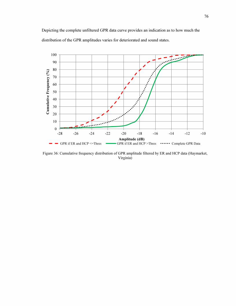
76

Depicting the complete unfiltered GPR data curve provides an indication as to how much the

distribution of the GPR amplitudes varies for deteriorated and sound states.

Figure 36: Cumulative frequency distribution of GPR amplitude filtered by ER and HCP data (Haymarket,

Virginia)

0

10

20

30

40

50

60

70

80

90

100

-28 -26 -24 -22 -20 -18 -16 -14 -12 -10

Cumulative Frequency (%)

Amplitude (dB)GPR if ER and HCP <=Thres GPR if ER and HCP >Thres Complete GPR Data

77

Figure 37: Cumulative frequency distribution of GPR amplitude filtered by ER and CD data (Haymarket,

Virginia)

Figure 38: Cumulative frequency distribution of GPR amplitude filtered by ER, HCP, and CD data

(Haymarket, Virginia)

0

10

20

30

40

50

60

70

80

90

100

-28 -26 -24 -22 -20 -18 -16 -14 -12 -10

Cumulative Frequency (%)

Amplitude (dB)

GPR if ER and CD <=Thres GPR if ER and CD >Thres Complete GPR Data

0

10

20

30

40

50

60

70

80

90

100

-28 -26 -24 -22 -20 -18 -16 -14 -12 -10

Cumulative Frequency (%)

Amplitude (dB)

GPR if ER, HCP, and CD <=Thres GPR if ER, HCP, and CD >Thres Complete GPR Data

78

Once the amplitudes have been filtered and cumulative frequency curves developed, the

difference between the deteriorated and sound curves is calculated (delta). The maximum delta

value indicates the amplitude at which its occurrence with deterioration is becoming insignificant

and its occurrence with a sound condition is becoming significant. For each filtering method, the

amplitudes of the three maximum delta values are averaged. The three average amplitude values

from the three filtering methods are then averaged together to identify the GPR threshold, as

rounded to the nearest 0.5 dB. Figure 39 provides the three delta curves for the GPR threshold

analysis performed on the bridge in Haymarket, Virginia. The ER and HCP filtering yielded a

value of −18.5 dB, ER and CD filtering resulted in −19 dB, and −18.5 dB for the ER, HCP, and

CD comparison. Averaging the three filtering results provides a GPR threshold amplitude of

−18.5 dB.

Figure 39: GPR threshold analysis delta curves (Haymarket, Virginia)

0

10

20

30

40

50

60

70

80

-28 -26 -24 -22 -20 -18 -16 -14 -12 -10

Delta

Amplitude (dB)

ER and HCP ER and CD ER, HCP, and CD

79

Some bridge decks do not have instances in which there is a severe delamination, active

corrosion, and corrosive environment at the same location. This occurs on bridges that are in

relatively good condition. If a structure does not have deteriorated and sound locations in one of

the ER/HCP, ER/CD, or ER/HCP/CD filters, then that filter will be removed from the threshold

analysis for that bridge. If the bridge is in such a condition that none of the filters have

deteriorated and sound locations, then the threshold will be defined by the average GPR

amplitude. Typically this will occur when a bridge is in very good condition and in which

instances of severe delamination are limited or nonexistent. The reason that the average GPR

amplitude is reserved as a fail-safe threshold identification method is that the calculated threshold

values identified for the rest of the bridges are very similar to their average GPR (Table 18).

They are typically within 0.5 dB of the average amplitude on that structure. Therefore, in

situations when the other analysis methods are not applicable, the average GPR amplitude will be

an initial threshold value.

Table 18: Comparison of GPR threshold values with average GPR amplitude

Carries Location GPR Threshold

(dB)

Average GPR Amplitude

(dB)

I-195 East Upper Freehold Township,

NJ -13.5 -13.9

Pequea

Boulevard Conestoga, PA -14.5 -14.5

State Route 123 Sandstone, MN -14.5 -14.1

State Route 15 Haymarket, VA -18.5 -18.0

State Route 21 Almond, NY -14.5 -13.7

State Route 93 Sumner, IA -12.5 -12.7

Application on Other Structures

The following section provides a sampling from the threshold analyses conducted on the other 11

bridges involved in this research. The objective of this section is to show how the data from the

80

other bridges was similar to and different from the bridge in Haymarket, Virginia, and how the

threshold identification methodology was refined by using the 11 other data sets. Table 19

provides an overview of the threshold values identified using the developed threshold

methodologies for the bridges in this study. The methods developed are robust statistical

methods that work on a variety of structures. However, there still remains extensive work to

validate the developed threshold methods by performing cores and autopsies to verify the

accuracy of the identified thresholds. In Table 19, some of the structures do not have a GPR

threshold because the GPR data for these structures were not available.

Table 19: Threshold analysis results

Carries Location ER Threshold

(kohm·cm)

HCP Active

Threshold

(mV CSE)

HCP Passive

Threshold

(mV CSE)

GPR

Threshold

(dB)

I-495 South Wilmington, DE 53 −350 −200 N/A

Interstate 195 Upper Freehold

Township, NJ 35 −350 −200 −13.5

Pequea

Boulevard Conestoga, PA 30 −425 −300 −14.5

School House

Road Middletown, PA 40 −350 −200 N/A

State Route

123 Sandstone, MN 45 -400 −200 −14.5

State Route 15 Haymarket, VA 45 −325 −250 −18.5

State Route 18 Neptune, NJ 45 −275 −175 N/A

State Route 21 Almond, NY 42 −325 −250 −14.5

State Route

273 Elkton, MD 35 −350 −250 N/A

State Route 47 Deptford

Township, NJ 47 −350 −200 N/A

State Route 93 Sumner, IA 35 −450 −375 −12.5

West Bangs

Ave Neptune, NJ 45 −250 −150 N/A

N/A – Data not available

81

Figure 40 is the slope of the filtered HCP data for the bridge in Sandstone, Minnesota. These data

illustrate the importance of using several resistivity filter values and taking an average of the

intersection points. The 5 kohm·cm filter has a significantly different intersection point with the

passive curves than do the other active curves. This happens when the bridge is in a relatively

good condition, meaning that there are very few locations of corrosive environment, resulting in

very few resistivity measurements below 30 kohm·cm. This makes the cumulative distribution

analysis dependent on fewer values, in turn making changes in slope more drastic.

Figure 40: Slope of the cumulative frequency distribution of filtered HCP data (Sandstone, Minnesota)

Figure 41 depicts the slope of the filtered data for the HCP threshold analysis on the bridge in

Elkton, Maryland. This data set provides tight curves for both passive and active data; however,

the passive curves rise ever so slightly before the active curves causing an intersection with the

active curves near −600 mV CSE. Clearly, these intersections are inconsequential to the

threshold and should not be included in the threshold identification. That is the reason the

0.00

0.05

0.10

0.15

0.20

0.25

0.30

0.35

0.40

0.45

0.50

0.55

0.60

0.65

-700 -600 -500 -400 -300 -200 -100 0

Slope

Half-Cell Potential (mV CSE)

5

10

15

20

25

30

70

75

80

85

90

95

82

program only starts to look for intersections after the slope has risen past a value of 0.05, and that

only one intersection between each curve is selected.

Figure 41: Slope of the cumulative frequency distribution of HCP data filtered according to resistivity

(Elkton, Maryland)

Figure 42 provides an example of why it is important to take the three maximum delta values

when performing the ER threshold analysis. The difference between the distributions of

resistivity for active and passive potential filtering is relatively small for the bridge in Almond,

New York. Therefore, in order to make sure the proper peak is picked and that one point is not

overly affecting the results, an average resistivity is calculated from the three highest delta values.

The three delta values are indicated in Figure 42 by the diamond markers. For this structure, the

threshold is 42 kohm·cm, which is very close to the resistivity at the absolute maximum delta

value of 40 kohm·cm.

0.0

0.1

0.2

0.3

0.4

0.5

0.6

0.7

0.8

0.9

1.0

-700 -600 -500 -400 -300 -200 -100 0

Slope

Half-Cell Potential (mV CSE)

5

10

15

20

25

30

70

75

80

85

90

95

83

Figure 42: Delta curve of filtered ER cumulative frequency data (Almond, New York)

Figure 43 presents the delta plot for the GPR analysis of the bridge in Sandstone, Minnesota.

This structure depicts the importance of using all three filtering methods, ER/HCP, ER/CD, and

ER/HCP/CD. There is much more variation between the three filtering methods for this bridge

than compared to the other bridges. By averaging the results of the three filtering methods, a

more accurate GPR threshold is identified; making sure that one filtering method is not

disproportionally affecting the results.

Figure 43: GPR threshold analysis delta curves (Sandstone, Minnisota)

0

2

4

6

8

10

12

14

16

18

20

0 20 40 60 80 100

Delta

Resistivity (kohm·cm)

0

10

20

30

40

50

60

-26 -24 -22 -20 -18 -16 -14 -12 -10 -8

Delta

Amplitude (dB)

ER and HCP ER and CD ER, HCP, and CD

84

The bridge in Upper Freehold, New Jersey has a limited amount of severe delaminations

identified by CD. Due to the limited amount of severe delaminations, the ER/CD and

ER/HCP/CD filters in the GPR threshold analysis do not provide any information (Figure 44).

Therefore, the GPR threshold for the bridge in Upper Freehold, New Jersey is based only on the

analysis of GPR amplitudes according to the ER/HCP filtering. This structure identifies the

importance of applying all three filtering methods in the GPR threshold analysis.

Figure 44: GPR threshold analysis delta curves (Upper Freehold Township, New Jersey)

CONDITION ASSESSMENT

Once the threshold values for each structure have been identified a damage-oriented condition

assessment of each structure can be developed. Figure 45 provides the condition assessment of

the bridge deck in Haymarket, Virginia. According to the CD and IE surveys, 22.5% of the deck

is severely delaminated and11.5% is delaminated/lateral cracking. Thus, there is a significant

portion of the deck, 34.0%, that is experiencing physical damage in the form of delamination. Of

0

5

10

15

20

25

30

35

40

45

-26 -24 -22 -20 -18 -16 -14 -12 -10 -8 -6 -4

Delta

Amplitude (dB)

ER and HCP ER and CD ER, HCP, and CD

85

the remaining deck area, 11.8% is actively corroding and 7.2% has a corrosive environment. The

remaining 47.0% of the deck is not experiencing any form of deterioration. Table 20 and Table

21 provide the amount of deck area in each damage state for each bridge. The bold values in

Table 20 and Table 21 are based on a complete multi-modal NDT analysis. For some of the

bridges, the IE and GPR data could not be gathered; therefore, the analysis could not be

completed for these bridges. A limited condition assessment using the available data was

undertaken for these structures and the results of those analyses are presented. The results not in

bold should be taken as an indication of the condition, but not as a complete assessment.

Table 20 provides the nonduplicating condition quantities for each bridge deck. The

nonduplicating area is a tabulation of the damage area when only the highest order of damage is

identified at each test location. Table 21 provides the duplicating condition quantities for each

structure. The duplicating area calculation counts the area of each damage type, regardless if that

area has been also counted in the area of another damage state.

The plots of each bridge’s condition assessment are located in Appendix 4 –Condition Plots of

Evaluated Bridges.

Figure 45: Condition assessment of Route 15 Bridge in Haymarket Virginia

86

Table 20: Nonduplicating condition quantities

Carries Location

Sound Corrosive

Environment

Active

Corrosion

Delamination/L

ateral Cracking

Severe

Delamination

Patches

(Duplicate w/

Sound)

ft2 % ft

2 % ft

2 % ft

2 % ft

2 % ft

2 %

I-495 South Wilmington, DE 11324 96.4 368 3.1 20 0.2 N/A N/A 36 0.3 0 0.0

I-195 East Upper Freehold

Township, NJ 1540 49.0 1136 36.2 24 0.8 132 4.2 308 9.8 0 0.0

Pequea

Boulevard Conestoga, PA 3160 46.0 1088 15.9 1308 19.1 N/A N/A 1308 19.1 116 1.7

School House

Road Middletown, PA 6920 66.6 3464 33.4 0 0.0 N/A N/A 0 0.0 0 0.0

State Route

123 Sandstone, MN 2180 33.9 736 11.4 496 7.7 1844 28.7 1176 18.3 0 0.0

State Route 15 Haymarket, VA 4884 47.0 748 7.2 1228 11.8 1192 11.5 2340 22.5 100 1.0

State Route 18 Neptune, NJ 2764 55.0 1144 22.8 1080 21.5 N/A N/A 36 0.7 52 1.0

State Route 21 Almond, NY 160 3.3 120 2.4 1564 31.8 2592 52.8 476 9.7 0 0.0

State Route

273 Elkton, MD 1640 41.0 380 9.5 1348 33.7 N/A N/A 628 15.7 12 0.3

State Route 47 Deptford

Township, NJ 8480 82.2 1748 16.9 80 0.8 N/A N/A 8 0.1 0 0.0

State Route 93 Sumner, IA 1000 34.0 140 4.8 364 12.4 312 10.6 1128 38.3 0 0.0

West Bangs

Ave Neptune, NJ 3888 65.9 1392 23.6 436 7.4 N/A N/A 188 3.2 60 1.0

N/A – Data not available

87

Table 21: Duplicating damage quantities

Carries Location

Sound Corrosive

Environment Active Corrosion

Delamination/L

ateral Cracking

Severe

Delamination Patches

ft2 % ft

2 % ft

2 % ft

2 % ft

2 % ft

2 %

I-495 South Wilmington, DE 11324 96.4 376 3.2 20 0.2 N/A N/A 36 0.3 0 0.0

I-195 East Upper Freehold

Township, NJ 1540 49.0 1588 50.6 48 1.5 132 4.2 308 9.8 0 0.0

Pequea

Boulevard Conestoga, PA 3160 46.0 3212 46.8 2028 29.5 N/A N/A 1308 19.1 620 9.0

School House

Road Middletown, PA 6920 66.6 3464 33.4 0 0.0 N/A N/A 0 0.0 0 0.0

State Route 123 Sandstone, MN 2180 33.9 4568 71.0 1944 30.2 1944 30.2 1176 18.3 0 0.0

State Route 15 Haymarket, VA 4884 47.0 6964 67.0 3816 36.7 1476 14.2 2340 22.5 204 2.0

State Route 18 Neptune, NJ 2764 55.0 1976 39.3 1100 21.9 N/A N/A 36 0.7 448 8.9

State Route 21 Almond, NY 160 3.3 4856 98.9 4428 90.1 2772 56.4 476 9.7 0 0.0

State Route 273 Elkton, MD 1640 41.0 1996 49.9 1868 46.7 N/A N/A 628 15.7 112 2.8

State Route 47 Deptford Township,

NJ 8480 82.2 1772 17.2 80 0.8 N/A N/A 8 0.1 0 0.0

State Route 93 Sumner, IA 1000 34.0 2468 83.8 1476 50.1 632 21.5 1128 38.3 0 0.0

West Bangs Ave Neptune, NJ 3888 65.9 1812 30.7 568 9.6 N/A N/A 188 3.2 416 7.0

N/A – Data not available

88

CONDITION RATING

The NBIS and AASHTO condition ratings for the 12 bridge decks in this study are provided in

Table 22 and Table 23. The most current NBIS rating, as determined by the last visual inspection

of each bridge by the bridge owner or its consultants, is listed in Table 22 along with the NBIS

rating as determined by the NDT data. Ratings with an asterisk were based on a limited analysis.

These bridges did not have IE and GPR data; therefore, the rating is not a completely accurate

representation of the deck condition or the entire multi-modal NDT algorithm. The NDT-

determined NBIS rating for each completed bridge produced a rating that was consistently one

value lower than reported NBIS ratings from most recent visual inspection. Of the ratings

performed on the structures with complete data sets, the I-195 East, Route 123, and Route 21

structures initially had an NBIS rating the same as the visual inspection. This was based purely

on the quantity of severe delaminations (CD & IE). However, these three bridges had large areas

of delamination/lateral cracking, active corrosion, and corrosive environment, which decreased

their rating by one due to the consideration of NDT inputs that reflect conditions that cannon be

discerned by visual inspection. The results of the NBIS condition rating using NDT data

indicates that there is more damage to these structures than was identified by visual inspection.

That is an expected result, since NDT provides a more in-depth assessment. This is why these

rating systems should incorporate NDT condition assessment, because they provide a more

complete and in-depth condition assessment beyond that visible through conventional inspection.

89

Table 22: NBIS rating according to NDT analysis

Carries Location NBIS from Visual

Inspection

NBIS from Multi-

Modal NDT

I-495 South Wilmington, DE 7 8*

I-195 East Upper Freehold Township, NJ 7 6

Pequea Boulevard Conestoga, PA 4 6*

School House Road Middletown, PA 8 8*

State Route 123 Sandstone, MN 6 5

State Route 15 Haymarket, VA 6 5

State Route 18 Neptune, NJ 6 8*

State Route 21 Almond, NY 7 6

State Route 273 Elkton, MD 6 5*

State Route 47 Deptford Township, NJ 7 8*

State Route 93 Sumner, IA 6 5

West Bangs Ave Neptune, NJ 7 7*

* Rating based on incomplete data

Table 23 provides the results of the AASHTO Bridge Element rating for the twelve bridge decks.

The values in Table 23 that are bold indicate results from a complete multi-modal NDT analysis.

The bridges that are not bold are missing IE and GPR results; therefore, those results are only a

partial depiction of the deck condition. For each AASHTO rating, the square footage and

percentage of the deck that fall into each category is provided. Since this method of deck rating

is a new addition to the DOT bridge inspection methodology, there is no historical information

that can be compared to these results. The AASHTO rating system does lend itself more easily to

accept NDT data; however, it is not a seamless transition and still requires adjustments.

90

Table 23: AASHTO condition rating results

Carries Location

Condition

State 1 (ft2

(%))

Condition

State 2 (ft2

(%))

Condition

State 3 (ft2

(%))

Condition

State 4 (ft2

(%))

I-495

South Wilmington, DE 11692 (99.5) 20 (0.2) 36 (0.3) 0 (0)

I-195 East Upper Freehold

Township, NJ 2736 (82.4) 320 (9.6) 264 (8.0) 0 (0)

Pequea

Boulevard Conestoga, PA 4248 (61.9) 1308 (19.1) 1308 (19.1) 0 (0)

School

House

Road

Middletown, PA 10384 (100) 0 (0.0) 0 (0.0) 0 (0)

State

Route 123 Sandstone, MN 2916 (45.3) 2340 (36.4) 1176 (18.3) 0 (0)

State

Route 15 Haymarket, VA 5632 (54.2) 2420 (23.3) 2340 (22.5) 0 (0)

State

Route 18 Neptune, NJ 3908 (77.8) 1080 (21.5) 36 (0.7) 0 (0)

State

Route 21 Almond, NY 280 (5.7) 4156 (84.6) 476 (9.7) 0 (0)

State

Route 273 Elkton, MD 2020 (50.5) 1348 (33.7) 628 (15.7) 0 (0)

State

Route 47

Deptford

Township, NJ 10228 (99.1) 80 (0.8) 8 (0.1) 0 (0)

State

Route 93 Sumner, IA 1140 (38.7) 676 (23.0) 1128 (38.3) 0 (0)

West

Bangs Ave Neptune, NJ 5280 (89.5) 436 (7.4) 188 (3.2) 0 (0)

A major benefit of approaching condition rating qualitatively with NDT methods is that it will

establish more consistent condition ratings. Visual inspection is very subjective; therefore, a

bridge surveyed by five different inspectors will yield slightly different results. However, with

NDT and its conversion to an NBIS and AASHTO rating system there is very limited subjectivity

in the data collection and analysis. This will improve constancy in bridge deck evaluations and

allow for better comparisons to be made between different bridge types and bridges owned by

different agencies.

DATA AGREEMENT RATING

The data agreement rating and the percentage of complete agreement for each bridge is provided

in Table 24. While complete agreement between all of the NDT methods is not expected, a level

91

of agreement is important, since some of the NDT methods measure related parameters. The

percentage of complete agreement values that have an asterisk beside them are based on analyses

conducted without IE and GPR data. The limited amount of data on these structures has

artificially inflated the data agreement values. They were included for completeness; however,

they do not reflect the true agreement for the deck. A data agreement rating was not produced for

the structures missing IE and GPR. The data agreement rating cannot be calculated for structures

that don’t have each condition state identified.

Of the completed structures, the bridge in Haymarket, Virginia has by far the highest level of

complete data agreement at 60.2% of the deck. It also received the highest data agreement rating

at 90.5. It is important to review both the agreement rating and the complete agreement

percentage, because a structure with a low percentage of complete agreement does not mean the

multi-modal NDT data is incorrect. If there was always complete agreement between all the

NDT methods, then the multi-modal NDT approach would not be necessary. These ratings show

that each NDT method is related, however, they are still detecting different damage states. Most

of the bridges have a data agreement rating of around 85 and a percentage of complete agreement

at approximately 40%. The data agreement rating and percentage of deck in complete agreement

can give an indication as to the cause of the identified deterioration. Since the methods utilized in

this study are highly affected by corrosion-induced deterioration, if there is significant agreement

between the methods, then that could indicate the primary cause of damage is due to corrosion.

On the other hand, if the agreement levels are low, this could indicate that the cause of the

damage is mechanical or some other type of deterioration mechanism.

92

Table 24: NDT data agreement rating and percentage of complete agreement

Carries Location Data Agreement

Rating

Percentage of Deck in

Complete Agreement

I-495 South Wilmington, DE N/A 99.6*

I-195 East Upper Freehold Township, NJ 84.0 39.5

Pequea Boulevard Conestoga, PA N/A 67.9*

School House Road Middletown, PA N/A 100.0*

State Route 123 Sandstone, MN 84.6 41.9

State Route 15 Haymarket, VA 90.5 60.2

State Route 18 Neptune, NJ N/A 94.3*

State Route 21 Almond, NY 82.9 23.5

State Route 273 Elkton, MD N/A 89.6*

State Route 47 Deptford Township, NJ N/A 99.4*

State Route 93 Sumner, IA 89.0 47.3

West Bangs Ave Neptune, NJ N/A 95.9*

N/A – Data not available * Based on limited NDT data

MULTI-MODAL CONDITION ASSESSMENT PROGRAM

As the final product of this research, a program was written to take processed multi-modal NDT

data and produce a complete condition assessment. Appendix 2 – MATLAB Code for Multi-

Modal Condition Assessment provides the MATLAB source code for the program. Appendix 3 –

Sample Output from Condition Assessment Code provides a sample of the output for the analysis

conducted on the bridge in Haymarket, Virginia.

The input file for the program is a tab-delimited text file that has the longitudinal and transverse

coordinates, along with the HCP, ER, IE, CD, GPR amplitude, and GPR cover depth data (Table

25). A requirement of the input file is that every line of data must have an entry for each column;

blank entries will cause an error. Figure 46 provides the input lines of code for the program.

Line 1 of the input code requires the location path for the data text file. The program takes the

text file and enters that data into individual MATLAB vectors. It is important that the order of

each data type in the text file match the first part of the input code, [long, tran, HCP, ER, IE, CD,

93

GPR, Cover], or an error will result. The data in the input text file should have the following

units; long and tran in ft, ER in kohm·cm, HCP in mV CSE, GPR in dB, IE in 1/2/3/4 signal

ratings, CD in 0/1, and Cover in inches. Line 2 of the input code recombines all the NDT data

into a MATLAB matrix. Lines 3 through 6 of the input code are general identification

information regarding the structure.

Table 25: Sample input file for the condition assessment program

4 1 -205 70 2 0 -17.0252 2.644

6 1 -180 58 4 1 -17.4291 2.385

8 1 -230 70 2 1 -16.9839 1.908

10 1 -225 53 2 0 -17.723 2.122

12 1 -235 59 1 0 -17.8039 1.908

14 1 -260 92 1 0 -17.6113 1.853

1) [long, tran, HCP, ER, IE, CD, GPR, Cover]=textread('C:\Research\VA 2009 NDE DATA Tab

Delimited.txt'); 2) DATA=[long, tran, HCP, ER, IE, CD, GPR, Cover]; 3) Carries='State Route 15'; 4) Spans='Interstate 66'; 5) State='Virginia'; 6) City='Haymarket';

Figure 46: Input information for the condition assessment code

Once the program accesses the input file, the first step the program takes is to identify each

threshold, ER, HCP, and GPR, according to the predefined methodology. Once the thresholds

have been identified, the program identifies the condition state of each location on the deck

according to the predefined damage states (Table 3). While the highest order of damage is the

most important, each damage state affecting each location is recorded. The program then

produces plotting files for each condition state, which can be input into the program SurferTM to

produce the final condition plot. The program will then calculate the area of the deck, duplicating

and nonduplicating, in each damage state. After the damage areas have been determined, then the

deck is rated using the NBIS and AASHTO methodologies. The program also calculates the data

94

agreement rating and the percentage of complete agreement. The program takes all of this

information and outputs it to a tab-delimited text file titled “ConditionAssessment.txt.” The

output text file is saved in the folder that is defined by MATLAB as the “current folder” during

the program run. The program is very versatile and is capable of producing a complete condition

assessment using multi-modal NDT data. The objective of this work is that as multi-modal NDT

becomes more common, this code will be utilized and expanded on by the NDT community. This

will greatly improve the effectiveness and accuracy of NDT condition assessment.

ALTERNATE GRID SPACING

An evaluation of grid spacing was conducted to establish whether NDT data collection could be

more efficient. The first grid spacing analysis conducted was on a small area of the Rt. 18 Bridge

in Neptune, New Jersey. Only ER and HCP measurements were made on this small grid. For

each grid spacing that was evaluated, the average and standard deviation of the data collected

were determined (Figure 47). The measured resistivity and potential values for each grid point

remained relatively consistent over the various grid spacings. The average change in measured

value from the 2 ft × 2 ft was 5.73 kohm·cm for ER and 39.4 mV CSE for HCP.

95

Figure 47: Analysis of ER and HCP measured values for changing survey grid spacing

An evaluation of the square footage of deck defined in each condition state according to each grid

spacing was also conducted. The condition states were: corrosive environment and active

corrosion as identified by ER and HCP. Based on the data collected on the bridge deck as a

whole, the threshold values were determined to be 45 kohm·cm for ER, −275 mV CSE for active

HCP, and −175 mV CSE for passive HCP. Using these threshold values, the area of the deck

below and above each threshold was determined using the various grid spacings (Figure 48). The

grid spacing had little effect on the amount of area that was in each condition category. The

average variation in square footage for the resistivity was 2.29 ft2 (2.4%) and the average

variation in the square footage of active HCP was 4.27 ft2 (6.2%). Overall the 2 ft × 2 ft grid

provides an effective grid density to identify the condition of a reinforced concrete bridge deck

when compared to a much smaller grid.

-500

-450

-400

-350

-300

-250

-200

-150

-100

0

20

40

60

80

100

120

140

0.0 0.5 1.0 1.5 2.0 2.5 3.0 3.5 4.0

Half-Cell Potential (mV CSE)

Resistivity (kohm·cm)/Resistivity (kohm·cm) and Half-

Cell Potential (mV) Standard Deviation

Grid Spacing (ft)

ER Average ER Standard DeviationHCP Standard Deviation HCP Average

96

Figure 48: Quantities of damage area based on grid spacing

Figure 49 and Figure 50 provide the results of the ER and HCP surveys using various grid

spacings. This helps to illustrate the effect that changing the grid spacing has on the NDT survey

results. Grid spacings of 0.5 ft × 0.5, 1.0 ft × 1.0, 1.5 ft × 1.5, and 2 ft × 2 ft were plotted for each

method. It is important to note that when plotting the information for the various grid spacings

only the data at the set intervals was input into the software to plot. While there is a clear loss of

detail as the grid spacings increase, the general evaluation of the deck area remains the same.

There is a large area of corrosive environment and active corrosion in the center of both surveys.

In the ER survey, the highly corrosive environment is surrounded by areas of still moderate

corrosive environment. In the HCP survey, the active corrosion region in the center is surrounded

by an area of uncretian corrosion activity. In all four plots, for both ER and HCP, the same

general conclusions result from the four different grid spacings; there is a large area of

deterioration in the center surounded by an area that has a moderate corrosive environment,

0

10

20

30

40

50

60

70

80

90

100

0.0 0.5 1.0 1.5 2.0 2.5 3.0 3.5 4.0

Area (ft2)

Grid Spacing (ft)

Corrosive Environment (ft2) Non-Corrosive Environment (ft2)

Active (ft2) Passive (ft2)

Transition (ft2)

97

however, corrosion activity has yet to initiate. This analysis shows that a 2 ft × 2 ft grid spacing

is an adequate spacing to provide an effective assessement of a reinforced concrete bridge deck.

Figure 49: ER survey results using various grid spacings (Rt. 18 Neptune, New Jersey)

98

Figure 50: HCP survey results using various grid spacings (Rt. 18 Neptune, New Jersey)

An analysis was also conducted on the previously surveyed bridge decks to evaluate the effect of

increasing the grid spacing past a 2 ft × 2 ft grid. For the 12 bridges that were a part of this

analysis, the effect of changing the grid size was evaluated on each of the bridges and the results

were averaged together. Figure 51 and Figure 52 plots the average change, compared to the 2 ft ×

2 ft grid, in area identified above and below the threshold for ER, HCP, and GPR. The x-axis

indicates the grid spacing increment; 2 ft × 2 ft is 2, 4 ft × 4 ft is 4, and so on. Figure 51 provides

the results of the square spacing; the spacing increment is indicated on the x-axis. Figure 52

provides the results of using rectangular grid spacing. Figure 51 indicates a clear increasing trend

in delta as the grid spacing increases. There is also a significant difference in the slope of areas

below and above the threshold. The slopes of the areas below threshold are much steeper than the

areas above threshold. This is due to the fact that areas of deterioration take up a smaller

99

proportion of most bridge decks, so when a change occurs in deteriorated area, it has a larger

effect on the percentage; whereas, a change in sound area has little effect on its percentage, since

it takes up a much larger percentage of the deck. In looking at the change in area identified as

sound, using a rectangular grid spacing (Figure 52) with 2 or 4 ft in the transverse direction and

up to 8 ft in the longitudinal direction has less than a 10% effect on the amount of area reported as

sound. This indicates that a grid spacing of 4 ft × 8 ft could be used on a bridge deck and would

still provide results that are within 10% of those of a 2 ft × 2 ft grid. If a larger 4 ft × 4 ft grid

was used on the bridge deck in Haymarket, Virginia, there would be a 73.6% (720 points)

reduction in test locations versus the 2 ft × 2 ft grid (2717 points).

Figure 51: Percent change in detection area of electrical methods for various square grid spacings

0

5

10

15

20

25

30

35

40

45

50

55

60

0 2 4 6 8 10 12 14 16 18 20

Delta (%)

Grid Spacing (ft)

ER Corrosive Environment

Area Delta %

ER Non-Corrosive

Environment Area Delta %

HCP Active Corrosion Area

Delta %

HCP Passive Corrosion Area

Delta %

GPR Degradation Area Delta

%

GPR Sound Area Delta %

100

Figure 52: Percent change in detection area of electrical methods for various rectangular grid spacings

Figure 53 and Figure 54 provides the results of the analysis of areas identified as deteriorated and

sound for the acoustic methods, IE and CD. Like the previous plot, the sound curves have a

much shallower slope than the deteriorated curves. For the acoustic methods, the change in

sound area stays below 5% for grid spacings as large as 4 ft × 8 ft and 6 ft × 6 ft. Due to the

small areas of severe delaminations, the effect that changing the grid spacing has on the CD

delaminated area is quite significant. The change in IE-identified areas of deterioration stays

below 10% for spacings up to 4 ft × 8 ft.

0

5

10

15

20

25

2x2 2x4 2x6 2x8 2x10 4x4 4x6 4x8 4x10

Delta (%)

Grid Spacing (ft)

ER Corrosive

Environment Area

Delta %

ER Non-Corrosive

Environment Area

Delta %

HCP Active

Corrosion Area Delta

%

HCP Passive

Corrosion Area Delta

%

GPR Degradation

Area Delta %

GPR Sound Area

Delta %

101

Figure 53: Percent change in detection area of acoustic methods for various square grid spacings

Figure 54: Percent change in detection area of acoustic methods for various rectangular grid spacings

0

5

10

15

20

25

30

35

40

45

50

55

60

0 2 4 6 8 10 12 14 16 18 20

Delta (%)

Grid Spacing (ft)

IE Rating 4 & 3 Area

Delta %

IE Rating 2 & 1 Area

Delta %

CD Delamination Area

Delta %

CD Sound Area Delta

%

0

5

10

15

20

25

30

35

40

45

2x2 2x4 2x6 2x8 2x10 4x4 4x6 4x8 4x10

Delta (%)

Grid Spacing (ft)

IE Rating 4 & 3

Area Delta %

IE Rating 2 & 1

Area Delta %

CD Delamination

Area Delta %

CD Sound Area

Delta %

102

Figure 55 provides the results of an analysis conducted to identify the effect that changing the

grid spacing has on the average ER, HCP, and GPR measured values on the bridge deck. This

figure includes both the square and rectangular grid spacings. Rectangular grid spacings are

indicated by using a decimal for the longitudinal dimension. For example, 2 ft × 6 ft is indicted

on the x-axis as 2.6. For grid spacings up to 4 ft × 8 ft there is less than 6% effect on the average

measurement. Like the previous results, increasing the grid spacing slightly, especially in the

longitudinal direction, has a limited effect on the results of the survey.

Figure 55: Percent change in average measurements due to various grid spacings

Figure 56 and Figure 57 provide a sampling of what the survey conducted on the Haymarket,

Virginia Bridge would look like if a 2 ft × 6 or 4 ft × 8 ft grid spacing were used for the ER or

HCP surveys. The most significant difference between the 2 ft × 2 ft grid spacing and the other

two plots is that in the 2 ft × 6 ft and 4 ft × 8 ft plots, the results look more granular. Since each

of these points must represent more of the deck in the longitudinal direction, they become

0

2

4

6

8

10

12

14

16

0 2 4 6 8 10 12 14 16 18 20

Delta (%)

Grid Spacing (ft)

Resistivity Average Delta %

Potential Average Delta %

Amplitude Average Delta %

103

elongated. While the look of the plots may be strange, the information presented in all three plots

for both technologies is very similar. The large areas of highly corrosive environment and active

corrosion are very similar among all three grid spacings. Due to the nature of how the data is

collected, there will clearly be areas of inflation and deflation relative to the true, however, the

overall assessment of the deck is very similar for the larger grid spacings. If the survey was

conducted using the 4 ft × 8 ft grid spacing, then the engineers would immediately know that this

bridge is in serious condition. They would also know that the area from about 30 to 150

longitudinally was in need of further investigation. Using a much larger grid spacing provides a

result that is similar enough to the much denser grid that a general condition assessment can still

be provided.

Figure 56: ER survey results using various grid spacings (Haymarket, Virginia)

104

Figure 57: HCP survey results using various grid spacings (Haymarket, Virginia)

As the grid spacing increases, the variation in the results follows a fairly linear trend throughout

the previous figures. However, the reductions in test locations for successively larger grid

spacings follow an exponential trend (Table 26). Even a small increase in grid spacing, from 2 ft

× 2 ft to 2 ft × 4 ft, causes a significant reduction in the amount of test locations, 49.8%. If such a

large decrease in testing locations will only affect the results by a few percent, then this is a

sizable benefit. A daytime lane closure for an NDT survey of a typical bridge deck is usually

constrained within the hours of 9:30 am and 2:30 pm; 5 hours. Assuming that, in that 5-hour

window, data is collected using a 2 ft × 2 ft grid, that same amount of area could be done by a 4 ft

× 4 ft grid in 1.3 hours and a 4 ft × 8 grid in 0.65 hours. This is a very sizable reduction in testing

time. This reduction in time would equate to considerable savings to the bridge owner.

105

Table 26: Percent reduction in amount of test points for various grids

Spacing 2×2 2×4 2×6 2×8 4×2 4×4 4×6 4×8

Reduction in Test Points (%) 0.0 49.8 66.3 74.6 48.7 74.3 82.7 87.0

The results of the grid analyses indicate that increasing the grid spacing can provide similar

results to a much denser 2 ft × 2 ft grid while significantly decreasing the amount of time required

for testing. The rectangular grid proved to be the most effective method at reducing the amount

of test locations while still maintaining a high level of accuracy. These results could be applied to

network level assessment of infrastructure, where quick evaluation of deck condition is necessary.

A large evaluation grid would allow for the categorization of each bridge’s deterioration level and

allow for decisions to be made regarding what structures need to be evaluated more closely and

what structures are in adequate condition.

FINDINGS

The results of this research lead to several findings regarding multi-modal NDT. The following

presents those findings.

• The areas of ER, HCP, and CD that indicated deterioration correlate well with areas of

highly attenuated GPR signal.

• An IE signal rating of 4 was associated with a decrease in measured values for the ER,

HCP, and GPR methods. When the IE signal rating was 1, 2, or 3, there was no clear

deviation in measured values.

• Various NDT methods indicated strong spatial agreement between the areas above and

below their respective thresholds. The methods that showed the strongest agreement

were ER/HCP, ER/GPR, CD/ER, CD/HCP, and CD/GPR.

106

• ER, HCP, GPR, and CD showed a high level of repeatability in measurements collected

on the same structure in different years. Areas of deterioration identified in the 2009

survey of the Haymarket, Virginia Bridge were also deteriorated in 2011.

• The correlations between ER, HCP, CD, and GPR can be used to identify threshold

values in ER, HCP, and GPR.

• Each bridge had a different level of agreement between the multi-modal NDT data. A

high level of data agreement is not necessary in understanding a bridge deck’s condition;

however, it did provide a higher confidence in the results. This form of analysis could be

used to help identify the deterioration mechanism that is affecting the bridge deck.

Corrosion-induced damage will have a high agreement rating, while damage caused from

a structural issue will have lower agreement.

CONCLUSIONS

This research was an in-depth analysis of multi-modal NDT condition assessment of bare

reinforced concrete bridge decks. It produced a wide array of results and procedures that will aid

in the further development of NDT condition assessment. The following presents the conclusions

reached as a result of this research.

• Strong correlations exist between ER and HCP measurements made on reinforced

concrete that suffers from chloride-induced corrosion. Areas that were indicated as

having a corrosive environment typically also indicated active corrosion.

• IE and CD showed an overall agreement regarding the identification of delaminations.

However, for strict comparison of CD indication of severe delamination, there was poor

agreement with IE.

107

• The steel reinforcing cover depth is an important factor in the service life of a structure.

Areas of low cover are more likely to experience deterioration sooner than areas of

deeper cover.

• Patches typically had the shallowest cover on a bridge deck when compared to areas of

severe delamination and sound concrete. Patch locations had delaminated in the past and

were repaired, indicating that cover depth plays an important factor in time-to-damage for

reinforced concrete.

• Areas of low resistivity lead to the future activation of corrosion. Locations with high

concentrations of moisture and chloride provide an environment that is favorable to

corrosion activity.

• According to the analyses conducted on the 12 bridge structures, resistivity less than 40

kohm·cm provides an environment that is favorable to corrosion activity.

• A location that is surrounded by highly deteriorated areas is more likely to become highly

deteriorated in the future than a location that is surrounded by sound concrete.

Reinforced concrete deterioration spreads over time to surrounding areas.

• A statistics-based approach to threshold identification provides a robust and versatile

method to identify threshold values on various structures.

• Due to the nature of chloride-induced corrosion, the NDT methods ER, HCP, GPR, IE,

and CD provide a detailed and complete assessment of reinforced concrete. These

methods together provide insight into the various forms of deterioration that occur during

the life of reinforced concrete.

• When providing a plot for condition assessment using contour plotting software, it is

important to understand exactly what the software is doing to the data and image.

Contouring software can create misleading information if done incorrectly and can create

false transitions between data sets.

108

• Rating a bridge deck using just visual inspection is not an adequate method of evaluation.

Significant deterioration may occur inside the concrete matrix that cannot be seen

through a purely visual inspection.

• Condition assessment using a multi-modal NDT approach is a complex process, however,

the developed software streamlines and automates a large portion of the process to help

create a more versatile and effective result.

• A grid spacing larger than 2 ft × 2 ft can provide an overall condition assessment that is

similar to a condition assessment provided by a 2 ft × 2 ft grid. Using a grid spacing of 2

ft × 6 ft or 4 ft × 8 ft significantly reduces the number of test locations and survey time,

while still maintaining an effective general condition assessment. These large grid

spacings can be used to quickly assess bridge conditions on a network level to identify

what bridges are in need of an in-depth assessment and what bridges are in adequate

condition.

RECOMMENDATIONS

Based on the results and conclusions of this research, the following recommendations regarding

bridge deck condition assessment and multi-modal NDT data collection have been made by the

author.

• Whenever possible, use a multi-modal NDT approach when evaluating reinforced

concrete. It is understood that not all the NDT methods utilized in this work can be

applied to every condition assessment project due to cost effectiveness and field-work

efficacy. However, it is important, when conducting a condition assessment, that more

than one NDT method is utilized so as to identify as many deterioration states as possible.

This will provide a more effective and complete condition assessment.

109

• It is recommended that when collecting, analyzing, and presenting ER, HCP, and GPR

data, that care is taken when applying threshold values. Threshold values presented in

literature are not absolutes; they shift based on many environmental factors. If the NDT

practitioner doesn’t have a firm understanding of the meaning of, and factors influencing,

measured values, then an improper condition assessment will be produced.

• With the development of a condition based assessment the next step of this research

should be to add the ability to forecast future damage. Predict the quantities of each

deterioration state for various time increments using established deterioration rate

research.

• NBIS and AASHTO Bridge Element ratings should adopt procedures to include NDT

information as a part of the condition rating. Having these rating systems change to

include NDT information is paramount for the future of bridge inspection and health

monitoring.

• It is recommended that when a network level condition assessment of a bridge deck is

required, that a rectangular grid spacing on the order of 2 ft × 6 ft or 4 ft × 8 ft be

implemented. Increasing the grid spacing like this will provide a more cost-effective

survey while still maintaining a reasonably effective condition assessment. A network

level condition assessment using a large grid will provide a general condition assessment

that will indicate if further evaluation action is needed on that structure.

FUTURE WORK

While working on this research project, there were several additional research topics of

importance and interest that became apparent. These ideas where not investigated as a part of this

work, since they were outside the scope. The following is a list of these ideas and topics which

merit further study.

110

• Autopsy of bridge deck samples to provide ground-truth verification for the threshold

methodology - While the threshold analysis methods were developed using sound

statistical analyses and known physical relationships, the inability to core into decks to

verify results limits it widespread application. The bridge in Haymarket, Virginia is

scheduled for replacement and would provide a great opportunity to collect ground-truth

information. Also, any new bridges that are surveyed using the multi-modal NDT

approach should be evaluated using this methodology to verify the methodology’s

applicability and provide any necessary adjustments.

• Further analysis into IE data and its relationship with the other NDT methods - The IE

data showed consistently the least amount of data correlation to the other NDT methods.

More work needs to be dedicated to understanding why.

• Evaluation of the deck condition surrounding patch locations - Ring anode effect is a

problem that leads to increased corrosion activity around patch locations. An analysis of

the condition data could provide insight into the seriousness of this problem and ways to

identify it.

• Work closely with DOT bridge inspectors and bridge policy officials to further develop

the NBIS and AASHTO deck ratings to gradually incorporate multi-modal NDT data -

Condition assessment of bridge decks is moving ever more into the realm of NDT and

these rating systems, which are federally mandated, should move towards adaptation of

NDT data.

• The NDT survey should be distributed and the results analyzed - The survey was not

completed due to difficulties in acquiring approval from the Rutgers Institutional Review

Board (IRB) at the Office of Research and Sponsored Programs. The Office of Research

and Sponsored Programs determined that the survey involved the collection of

information from human subjects, which requires the Human Subjects Certification

111

Program (HSCP) to be completed by all researchers involved. Due to difficulties in this

approval process, the survey was not approved in time to receive responses prior to the

submission of this work. Therefore, the results of the survey were not presented as a part

of this work and should be completed as future work.

112

REFERENCES

AASHTO. AASHTO Guide Manual for Bridge Element Inspection. 2011.

ACI Committee 222. Corrosion of Prestressing Steels. American Concrete Institute, 2001.

ACI Committee 222. Protection of Metals in Concrete Against Corrosion. American Concrete

Institute, 2001.

ASTM. Standard Practice for Measuring Delaminations in Concrete Bridge Decks by Sounding.

ASTM, 1992.

ASTM. Standard Test Method for Corrosion Potentials of Uncoated Reinforcing Steel in

Concrete. ASTM, 2009.

Broomfield, J. P. Corrosion of Steel in Concrete. Abingdon, Oxon: Taylor & Francis, 2007.

Bungey, J. H. Testing of Concrete in Structures. 2. New York, New York: Chapman & Hall,

1989.

Daniels, D. Ground Penetrating Radar. 2. London: The Institution of Engineering and

Technology, 2004.

Elkey, W., and E. J. Sellevold. Electrical Resistivity of Concrete. Oslo: Norwegian Road

Research Laboratory, 1995.

Elsener, B., C. Andrade, J. Gulikers, R. Polder, and M. Raupach. "Half-Cell Potential

Measurements - Potential Mapping on Reinforced Concrete Structures." Materials and Structures

36 (August-September 2003): 461-471.

Feliu, S., J. A. Gonzalez, and C. Andrade. "Electrochemical Methods for On-Site Determinations

of Corrosion Rates of Rebars." In Corrosion Activity of Steel Reinforced Concrete Structures, by

N. S. Berke, E. Escalante, C. K. Nmai and D. Whiting, 107-118. West Conshohocken,

Pennsylvania: ASTM International, 1996.

Funahashi, M. "Predicting Corrosion-Free Service Life of a Concrete Structure in a Chloride

Environment." Materials Journal (ACI) 87, no. 6 (November 1990): 581-587.

Gros, X. E., J. Bousigue, and K. Takahashi. "NDT data fusion at pixel level." (NDT&E

International) 32 (1999): 283-292.

Gu, P., and J. J. Beaudoin. "Obtaining Effective Half-Cell Potential Measurements in Reinforced

Concrete Structures." Construction Technology Update (Institute for Research in Construction),

July 1998: 1-4.

Gucunski, N., et al. Nondestructive Testing to Identify Concrete Bridge Deck Deterioration.

Washington, D.C.: Transportation Resarch Board, 2013.

Gucunski, N., F. Romero, S. Kruschwitz, and R. Feldmann. "Comparative Study of Bridge Deck

Deterioration Detection and Characterization by Multiple NDE Methods." Edinburgh: Structural

Faults & Repair, 2010.

Gucunski, N., F. Romero, S. Kruschwitz, R. Feldmann, A. Abu-Hawash, and M. Dunn. "Multiple

Complementary Nondestructive Evaluation Technologies for Condition Assessment of Concrete

113

Bridge Decks." Transportation Research Record: Journal of the Transportation Research Board

(Transportation Research Board of the National Academies), no. 2201 (December 2010): 34-44.

Gucunski, N., G. Slabaugh, Z. Wang, T. Fang, and A. Maher. "Visualization and Interpretation of

Impact Echo Data from Bridge Deck Testing." Journal of Transportation Research Board

(Transportation Research Board), 2007.

Gucunski, N., R. Feldmann, F. Romero, S. Kruschwitz, A. Abu-Hawash, and M. Dunn.

"Multimodal condition assessment of bridge decks by NDE and its validation." Mid-Continent

Transporation Research Symposium. Ames: Iowa State University, 2009.

Gucunski, N., R. Feldmann, F. Romero, S. Kruschwitz, and H. Parvardeh. "Comprehensive

Condition Assessment of Bridge Decks by Multimodal NDE." Nondestructive Characterization

for Composite Materials, Aerospace Engineering, Civil Infrastructure, and Homeland Security.

San Diego, 2010.

Henderson, M. E., G. N. Dion, and R. D. Costley. "Acoustic Inspection of Concrete Bridge

Decks." Newport Beach: Nondestructive Evaluation of Bridges and Highways III, 1999.

Horn, D. "Reliability Analysis Combining Multiple Inspection Techniques." Berlin: ECNDT,

2006.

Huston, D., J. Cui, D. Burns, and D. Hurley. "Concrete Bridge Deck Condition Assessment with

Automated Multisensor Techniques." Structure and Infrastructure Engineering, 2010: 1-11.

Huston, D., P. Fuhr, K. Maser, and W. Weedon. "Nondestructive Testing of Reinforced Concrete

Bridges Using Radar Imaging Techniques." The New England Transportation Consortium

Report, 2002.

Kansas Department of Transportation Bureau of Local Projects Bridge Team. Bridge Inspection

Manual. Topeka: Kansas Department of Transporation, 2012.

Kessler, R. J., R. G. Powers, E. Vivas, M. A. Paredes, and Y. P. Virmani. Surface Resistivity as

an Indicator of Concrete Chloride Penetration Resistance. Skokie: Concrete Bridge Council,

2008.

Kohl, C., and D. Streicher. "Results of reconstructed and fused NDT-data measured in the

laboratory and on-site at bridges." (Cement & Concrete Composites) 28 (2006).

Krauss, P. D., J. S. Lawler, and K. A. Steiner. Guidelines for Selection of Bridge Deck Overlays,

Sealers and Treatments. National Cooperative Highway Research Program Transportation

Research Board of The National Academies, 2008.

Maierhofer, C., G. Zacher, C. Kohl, and J. Wostmann. "Evaluation of Radar and Complementary

Echo Methods for NDT of Concrete Elements." (Journal of Nondestructive Evaluation) 27

(2008).

Malhotra, V. M., and N. J. Carino. Handbook on Nondestructive Testing of Concrete. 2. West

Cohshohocken, Pennsylvania: ASTM International, 2004.

McCafferty, E. Introduction to Corrosion Science. New York: Springer, 2010.

114

Morris, W., A. Vico, M. Vazquez, and S. R. de Sanchez. "Corrosion of Reinforcing Steel

Evaluated by Means of Concrete Resistivity Measurements." Corrosion Science 44 (2002): 81-

99.

New Jersey Department of Transportation. Design Manual for Bridges and Structures. 5th.

Trenton: New Jersey Department of Transportation, 2009.

Parrillo, R., and R. Roberts. "Bridge Deck Condition Assessment Using Ground Penetrating

Radar." Ninth European Conference on NDT. Berlin, 2006.

Poulsen, E., and L. Mejlbro. Diffusion of Chloride in Concrete: Theory and Application. New

York, New York: Taylor & Francis, 2006.

Rapa, M., and W. H. Hartt. "Non-Destructive Evaluation of Jacketed Pre-Stressed Concrete Piles

for Corrosion Damage." NACE, 1999.

Ryan, T., R. Hartle, J. Mann, and L. Danovich. Bridge Inspector's Reference Manual. Federal

Highway Administration, U.S. Department of Transportation, 2006.

Virginia Department of Transporation. Manuals of the Structure and Bridge Division. Richmond:

Virginia Department of Transporation, 2012.

Virginia Department of Transportation. Element Data Collection Manual. Richmond: Virginia

Department of Transportation, 2007.

ACKNOWLEDGEMENT OF PREVIOUS PUBLICATION

Pailes, B.M., and Gucunski, N., “Statistical Correlation Method to Identify Half-Cell Potential

and Electrical Resistivity Threshold Values,” Transportation Research Board 93nd Annual

Meeting, Washington, D.C., January 2014.

Pailes, B.M., Gucunski, N., and Brown, M.C., “Correlation of Non-Destructive Testing Results to

Improve Assessment of Corrosion and Corrosion Damage of a Reinforced Concrete Deck,”

Transportation Research Board 92nd Annual Meeting, Washington, D.C., January 2013

115

APPENDICES

116

APPENDIX 1 – NON-DESTRUCTIVE TEST METHOD SURVEY

117

118

119

APPENDIX 2 – MATLAB CODE FOR MULTI-MODAL CONDITION ASSESSMENT

120

%-----Condition Assesment----------------------------------------------

---%

%Program by Brian M. Pailes 10/15/2013 %Inputs %HCP - Values are in mV %ER - Values are in kohm*cm %GPR - Values are in dB %CD - 1 for delamination 0 for no delamination %Once thresholds have been identified convert it into plotable

condition data %[HCP,ER, GPR]=textread('filename'); %DATA=[HCP,ER, GPR]; %Importing Data from research %MN Pilot Bridge NDE data %[long, tran, HCP, ER, IE, Cover, GPR, CD]=textread('C:\Users\Brian

Pailes\Documents\Brian Pailes\Rutgers University\Research\Data\LTBP\MN

LTBP Data\MN NDE DATA Tab Delimited.txt'); %DATA=[long, tran, HCP, ER, IE, CD, GPR, Cover]; %Carries='State Route 123'; %Spans='Kettle River'; %State='Minnesota'; %City='Sandstone'; %NY Pilot Bridge NDE Data %[long, tran, HCP, ER, IE, Cover,GPR,PSPA,CD]=textread('C:\Users\Brian

Pailes\Documents\Brian Pailes\Rutgers University\Research\Data\LTBP\NY

LTBP Data\NY NDE DATA Tab Delimited.txt'); %DATA=[long, tran, HCP, ER, IE, CD, GPR, Cover]; %Carries='State Route 21'; %Spans='Karr Valley Creek'; %State='New York'; %City='Almond'; %NJ Pilot Bridge NDE Data %[long, tran, HCP, ER,IE,Cover,GPR,PSPA,CD]=textread('C:\Users\Brian

Pailes\Documents\Brian Pailes\Rutgers University\Research\Data\LTBP\NJ

LTBP Data\NJ NDE DATA Tab Delimited.txt'); %DATA=[long, tran, HCP, ER, IE, CD, GPR, Cover]; %Carries='Interstate 195 East'; %Spans='Sharon Station Road'; %State='New Jersey'; %City='Upper Freehold Township'; %O2 Sumner Iowa Bridge NDE Data %[long, tran, HCP, ER,IE,Cover,GPR,PSPA,CD]=textread('C:\Users\Brian

Pailes\Documents\Brian Pailes\Rutgers University\Research\Data\Iowa\O2

NDE DATA Tab Delimited.txt');

121

%DATA=[long, tran, HCP, ER, IE, CD, GPR, Cover]; %Carries='State Route 93'; %Spans='Natural Stream'; %State='Iowa'; %City='Sumner'; %O5 Indian Creek Iowa NO GPR DATA %[long, tran, ER, HCP]=textread('C:\Users\Brian Pailes\Documents\Brian

Pailes\Rutgers University\Research\Data\Iowa\O5 NDE DATA Tab

Delimited.txt'); %DATA=[long, tran, HCP, ER, IE, CD, GPR, Cover]; %Carries=''; %Spans=''; %State='Iowa'; %City=''; %O6 Villisca Iowa NO GPR DATA %[long, tran, ER, HCP]=textread('C:\Users\Brian Pailes\Documents\Brian

Pailes\Rutgers University\Research\Data\Iowa\O6 NDE DATA Tab

Delimited.txt'); %DATA=[long, tran, HCP, ER, IE, CD, GPR, Cover]; %Carries=''; %Spans=''; %State='Iowa'; %City=''; %I495 Wilmington DE %[long, tran, HCP, ER]=textread('C:\Users\Brian Pailes\Documents\Brian

Pailes\Rutgers University\Research\Data\LTBP\I 495 South over Rt 13-

Wilmington DE\I495 NDE DATA Tab Delimited.txt'); %DATA=[long, tran, HCP, ER, IE, CD, GPR, Cover]; %Carries='Interstate 495 South'; %Spans='Route 13'; %State='Delaware'; %City='Wilmington'; %Pequea Blvd Conestoga PA %[long, tran, HCP, ER]=textread('C:\Users\Brian Pailes\Documents\Brian

Pailes\Rutgers University\Research\Data\LTBP\Pequea Blvd over Pequea

Creek-Conestoga PA\Pequea Blvd NDE DATA Tab Delimited.txt'); %DATA=[long, tran, HCP, ER, IE, CD, GPR, Cover]; %Carries='Pequea Boulevard'; %Spans='Pequea Creek'; %State='Pennsylvania'; %City='Conestoga'; %Rt 18 Neptune NJ %[long, tran, HCP, ER]=textread('C:\Users\Brian Pailes\Documents\Brian

Pailes\Rutgers University\Research\Data\LTBP\Rt 18 over Rt 66-Neptune

NJ\Rt 18 NDE DATA Tab Delimited.txt'); %DATA=[long, tran, HCP, ER, IE, CD, GPR, Cover]; %Carries='State Route 18'; %Spans='State Route 66'; %State='New Jersey'; %City='Neptune';

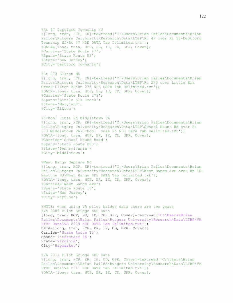
122

%Rt 47 Deptford Township NJ %[long, tran, HCP, ER]=textread('C:\Users\Brian Pailes\Documents\Brian

Pailes\Rutgers University\Research\Data\LTBP\Rt 47 over Rt 55-Deptford

Township NJ\Rt 47 NDE DATA Tab Delimited.txt'); %DATA=[long, tran, HCP, ER, IE, CD, GPR, Cover]; %Carries='State Route 47'; %Spans='State Route 55'; %State='New Jersey'; %City='Deptford Township'; %Rt 273 Elkton MD %[long, tran, HCP, ER]=textread('C:\Users\Brian Pailes\Documents\Brian

Pailes\Rutgers University\Research\Data\LTBP\Rt 273 over Little Elk

Creek-Elkton MD\Rt 273 NDE DATA Tab Delimited.txt'); %DATA=[long, tran, HCP, ER, IE, CD, GPR, Cover]; %Carries='State Route 273'; %Spans='Little Elk Creek'; %State='Maryland'; %City='Elkton'; %School House Rd Middletown PA %[long, tran, HCP, ER]=textread('C:\Users\Brian Pailes\Documents\Brian

Pailes\Rutgers University\Research\Data\LTBP\School House Rd over Rt

283-Middletown PA\School House Rd NDE DATA Tab Delimited.txt'); %DATA=[long, tran, HCP, ER, IE, CD, GPR, Cover]; %Carries='School House Road'; %Spans='State Route 283'; %State='Pennsylvania'; %City='Middletown'; %West Bangs Neptune NJ %[long, tran, HCP, ER]=textread('C:\Users\Brian Pailes\Documents\Brian

Pailes\Rutgers University\Research\Data\LTBP\West Bangs Ave over Rt 18-

Neptune NJ\West Bangs NDE DATA Tab Delimited.txt'); %DATA=[long, tran, HCP, ER, IE, CD, GPR, Cover]; %Carries='West Bangs Ave'; %Spans='State Route 18'; %State='New Jersey'; %City='Neptune'; %NOTE: when using VA pilot bridge data there are two years %VA 2009 Pilot Bridge NDE Data [long, tran, HCP, ER, IE, CD, GPR, Cover]=textread('C:\Users\Brian

Pailes\Documents\Brian Pailes\Rutgers University\Research\Data\LTBP\VA

LTBP Data\VA 2009 NDE DATA Tab Delimited.txt'); DATA=[long, tran, HCP, ER, IE, CD, GPR, Cover]; Carries='State Route 15'; Spans='Interstate 66'; State='Virginia'; City='Haymarket'; %VA 2011 Pilot Bridge NDE Data %[long, tran, HCP, ER, IE, CD, GPR, Cover]=textread('C:\Users\Brian

Pailes\Documents\Brian Pailes\Rutgers University\Research\Data\LTBP\VA

LTBP Data\VA 2011 NDE DATA Tab Delimited.txt'); %DATA=[long, tran, HCP, ER, IE, CD, GPR, Cover];

123

%Carries='State Route 15'; %Spans='Interstate 66'; %State='Virginia'; %City='Haymarket'; %False Data used to check code %[long, tran, HCP, ER,IE,Cover,GPR,PSPA,CD]=textread('C:\Users\Brian

Pailes\Documents\Brian Pailes\Rutgers University\Research\Data\FAKE

BRIDGE DECK DATA Tab Delimited.txt'); %DATA=[long, tran, HCP, ER,IE,Cover,GPR,PSPA,CD]; %determines number of data points [AA,BB]=size(DATA); %-----HCP Threshold Analysis-------------------------------------------

---% %Filters HCP data based on the ER value at the same test location %Defines the "active" end of the ER scale k=1; ERlowlimit=30; ERlow=5; ERinc=5; ERnum=((ERlowlimit-ERlow)/ERinc)+1; %Filters out the HCP data based on the ER value and increments while(ERlow<=ERlowlimit) j=1; i=1; while(j<=AA) if(ER(j,1)<=ERlow) HCPActiveValues(i,k)=HCP(j,1); i=i+1; else i=i; end j=j+1; end istore(k,1)=i; ERlow=ERlow+ERinc; k=k+1; end %Defines the "passive" end of the ER scale [ii,kk]=size(HCPActiveValues); k=1+kk; ERhighlimit=95; ERhigh=70; ERinc=5; ERnum=((ERhighlimit-ERhigh)/ERinc)+1; while(ERhigh<=ERhighlimit) j=1;

124

i=1; while(j<=AA) if(ER(j,1)>=ERhigh) HCPActiveValues(i,k)=HCP(j,1); i=i+1; else i=i; end j=j+1; end istore(k,1)=i; ERhigh=ERhigh+ERinc; k=k+1; end %Resets high and low limit on ER filtering ERlow=5; ERhigh=70; %Replaces any zeros that are artificially entered into the matrix

with 99999 [ii,jj]=size(HCPActiveValues); maxval=max(istore); k=1; while(k<=jj) i=istore(k,1); while(i<maxval) HCPActiveValues(i,k)=99999; i=i+1; end k=k+1; end %Creates the bins for the frequency analysis i=1; HCPBinHigh=60; HCPBinLow=-700; HCPBinInc=38; HCPBinCorection=HCPBinInc/2; while(HCPBinLow<=HCPBinHigh) HCPBins(i,1)=HCPBinLow-HCPBinCorection; HCPBinLow=HCPBinLow+HCPBinInc; i=i+1; end HCPBins(21,1)=90000; %frequency analysis HCPfreq=hist(HCPActiveValues,HCPBins); %Removes the 99999 values entered earlier [ii,jj]=size(HCPfreq); k=1; while(k<=jj) i=1; while(i<ii)

125

HCPfreqreal(i,k)=HCPfreq(i,k); i=i+1; end k=k+1; end %Calculation of cumulative frequency [ii,jj]=size(HCPfreqreal); k=1; while(k<=jj) i=1; while(i<=ii) j=i-1; if(i==1) HCPcummlative(i,k)=HCPfreqreal(i,k); else HCPcummlative(i,k)=HCPfreqreal(i,k)+HCPcummlative(j,k); end i=i+1; end k=k+1; end %Turning cummulative frequency into a percent HCPsum=sum(HCPfreqreal); [ii,jj]=size(HCPcummlative); k=1; while(k<=jj) i=1; while(i<=ii)

HCPcummlativepercent(i,k)=(HCPcummlative(i,k)/HCPsum(1,k))*100; i=i+1; end k=k+1; end %Calculation of first derivative [ii,jj]=size(HCPcummlativepercent); k=1; while(k<=jj) i=2; while(i<ii) j=i+1; m=i-1; HCPFirstDerivative(i,k)=(HCPcummlativepercent(j,k)-

HCPcummlativepercent(m,k))/(2*HCPBinInc); i=i+1; end k=k+1; end %Creating a matrix for the ER's increments used in filtering i=1;

126

ERvalue=ERlow; while(ERvalue<=ERlowlimit) ERBinsforHCP(i,1)=ERvalue; ERvalue=ERinc+ERvalue; i=i+1; end ERvalue=ERhigh; while(ERvalue<=ERhighlimit) ERBinsforHCP(i,1)=ERvalue; ERvalue=ERinc+ERvalue; i=i+1; end %Check to see if each ER filter has HCP values in it [ii,jj]=size(HCPcummlative); j=1; while(j<=jj) aCheck=HCPcummlative(ii,j); if(aCheck>0) HCPcheck=1; else HCPcheck=0; j=jj; end j=j+1; end if(HCPcheck==1) %Determining where first derivative of the "active" ER filters

crosses %"passive" ER filter ERnumlow=((ERlowlimit-ERlow)/ERinc)+1; ERnumhigh=((ERhighlimit-ERhigh)/ERinc)+1; %Locate location to start intersection identification [ii,jj]=size(HCPFirstDerivative); j=1; while(j<=6) i=1; while(i<=ii) Startvalue=HCPFirstDerivative(i,j); if(Startvalue>=.05) if(j==1) Start5=i; elseif(j==2) Start10=i; elseif(j==3) Start15=i; elseif(j==4) Start20=i; elseif(j==5) Start25=i; else Start30=i;

127

end i=ii+1; else i=i+1; end end j=j+1; end [ii,jj]=size(HCPFirstDerivative); k=1; w=1; while(k<=ERnumlow) m=ERnumlow+1; while(m<=ERnumhigh+ERnumlow) if(k==1) i=Start5; elseif(k==2) i=Start10; elseif(k==3) i=Start15; elseif(k==4) i=Start20; elseif(k==5) i=Start25; else i=Start30; end while(i<ii) j=i+1; n=2; x1=HCPBins(i,1)+HCPBinCorection; y1=HCPFirstDerivative(i,k); x2=HCPBins(j,1)+HCPBinCorection; y2=HCPFirstDerivative(j,k); while(n<ii) p=n+1; u1=HCPBins(n,1)+HCPBinCorection; v1=HCPFirstDerivative(n,m); u2=HCPBins(p,1)+HCPBinCorection; v2=HCPFirstDerivative(p,m); if(x1==x2) i=i; elseif(u1==u2) i=i; else b1=(y2-y1)/(x2-x1); b2=(v2-v1)/(u2-u1); a1=y1-b1*x1; a2=v1-b2*u1; if(b1==b2) i=i; else

128

xi=(a2-a1)/(b1-b2); yi=b1*xi+a1; check1=(x1-xi)*(xi-x2); check2=(u1-xi)*(xi-u2); if(check1>=0)&&(check2>=0)&&(abs(yi)>0)

HCPintersection(w,1)=HCPBins(i,1)+HCPBinCorection;

HCPintersection(w,2)=HCPFirstDerivative(i,k);

HCPintersection(w,3)=HCPBins(j,1)+HCPBinCorection;

HCPintersection(w,4)=HCPFirstDerivative(j,k);

HCPintersection(w,5)=HCPBins(n,1)+HCPBinCorection;

HCPintersection(w,6)=HCPFirstDerivative(n,m);

HCPintersection(w,7)=HCPBins(p,1)+HCPBinCorection;

HCPintersection(w,8)=HCPFirstDerivative(p,m); HCPintersection(w,9)=xi; HCPintersection(w,10)=yi; HCPintersection(w,11)=k; HCPintersection(w,12)=m; w=w+1; else i=i; end end end n=n+1; end i=i+1; end m=m+1; end k=k+1; end %If there are multiple intersections by one curve with anouther it

selects %only 1 i=1; [ii,jj]=size(HCPintersection); while(i<ii) j=i+1; mean1=mean(HCPintersection); mean11=mean1(1,9);

129

if(HCPintersection(i,11)==HCPintersection(j,11))&&(HCPintersection(i,12

)==HCPintersection(j,12)) Delta1=abs(mean11-HCPintersection(i,9)); Delta2=abs(mean11-HCPintersection(j,9)); if(Delta1<Delta2)

HCPintersection=HCPintersection(setdiff(1:size(HCPintersection,1),[j]),

:); else

HCPintersection=HCPintersection(setdiff(1:size(HCPintersection,1),[i]),

:); end i=i; [ii,jj]=size(HCPintersection); else i=i+1; end end %Determines the active threshold rounded to the nearest integer of

25 sum11=0; i=1; [ii,jj]=size(HCPintersection); while(i<=ii) sum11=HCPintersection(i,9)+sum11; i=i+1; end HCPActiveRAW=sum11/ii; HCPRemainder=HCPActiveRAW/25; HCPfactor=round(HCPRemainder); HCPActive=HCPfactor*25; %The method of finding the passive threshold will be when the slope %of cumulative frequency plot for low ER values gets below 0.025. %Primary method of passive threshold analysis [ii,jj]=size(HCPFirstDerivative); k=1; while(k<=jj) [ii,jj]=size(HCPFirstDerivative); while(ii>1) if(abs(HCPFirstDerivative(ii,k))<0.025) ii=ii-1; else ii=ii+1; HCPSecondLimit(1,k)=HCPBins(ii,1)+HCPBinCorection; ii=1; end end k=k+1;

130

end %Determine which method of passive threshold analysis to use sum1=0; i=1; while(i<=ERnumlow) sum1=HCPSecondLimit(1,i)+sum1; i=i+1; end HCPPassiveRAW=sum1/ERnumlow; HCPRemainder=HCPPassiveRAW/25; HCPfactor=round(HCPRemainder); HCPPassive=HCPfactor*25; %If the passive threshold is abnormally low, then rechecking the

threshold %using a slope of 0.05 if(HCPPassive>-100) [ii,jj]=size(HCPFirstDerivative); k=1; while(k<=jj) [ii,jj]=size(HCPFirstDerivative); while(ii>1) if(abs(HCPFirstDerivative(ii,k))<0.05) ii=ii-1; else ii=ii+1; HCPSecondLimit2(1,k)=HCPBins(ii,1)+HCPBinCorection; ii=1; end end k=k+1; end sum2=0; i=1; while(i<=ERnumlow) sum2=HCPSecondLimit2(1,i)+sum2; i=i+1; end HCPPassiveRAW=sum2/ERnumlow; HCPRemainder=HCPPassiveRAW/25; HCPfactor=round(HCPRemainder); HCPPassive=HCPfactor*25; else end str1=sprintf('The threshold for active corrosion is %d mV',

HCPActive);

131

str2=sprintf('The threshold for passive condition is %d mV',

HCPPassive); disp(str1); disp(str2); else HCPActive=-350; HCPPassive=-200; disp('The deck has ER values that indicate a deck in excellent

condition'); disp('There are not enough low ER values to perform this

analysis'); disp('The HCP threshold values will be set as default values'); str1=sprintf('The threshold for active corrosion is %d mV',

HCPActive); str2=sprintf('The threshold for passive condition is %d mV',

HCPPassive); disp(str1); disp(str2); end %-----ER Threshold Analysis----------------------------------------

-------% [AA,BB]=size(DATA); %Creates the ER Bins for cumulative frequency ERlow=5; ERhigh=100; ERinc=5; ERbincor=ERinc/2; num=((ERhigh-ERlow)/ERinc)+1; i=1; k=ERlow; while(i<=num) ERBins(i,1)=k-ERbincor; k=k+ERinc; i=i+1; end %Filters ER data if HCP is less than equal to active threshold indicatorER1=0; i=1; k=1; while(i<=AA) if(HCP(i,1)<=HCPActive) ERActive(k,1)=ER(i,1); k=k+1; i=i+1; indicatorER1=1; else i=i+1;

132

end end %Filters ER data if HCP is greater than equal to passive threshold indicatorER2=0; i=1; k=1; while(i<=AA) if(HCP(i,1)>=HCPPassive) ERPassive(k,1)=ER(i,1); k=k+1; i=i+1; indicatorER2=1; else i=i+1; end end if(indicatorER1==1)&&(indicatorER2==1) FAILer=1; %Frequency analysis ERfreqactive=hist(ERActive,ERBins); ERfreqactive=transpose(ERfreqactive); ERfreqpassive=hist(ERPassive,ERBins); ERfreqpassive=transpose(ERfreqpassive); %Calculation of cumulative frequency %Note: analysis excludes last row, this is frequency of ER values

over 99 %which are statistically higher due to limits of ER device [ii,jj]=size(ERfreqactive); i=1; while(i<ii) if(i==1) ERcumlativeActive(i,1)=ERfreqactive(i,1); else j=i-1;

ERcumlativeActive(i,1)=ERfreqactive(i,1)+ERcumlativeActive(j,1); end i=i+1; end [ii,jj]=size(ERfreqpassive); i=1; while(i<ii) if(i==1) ERcumlativePassive(i,1)=ERfreqpassive(i,1); else j=i-1;

ERcumlativePassive(i,1)=ERfreqpassive(i,1)+ERcumlativePassive(j,1); end i=i+1; end

133

%Turning cumulative frequency into a percent [ii,jj]=size(ERfreqactive); sumA=sum(ERfreqactive)-ERfreqactive(ii,jj); [ii,jj]=size(ERcumlativeActive); i=1; while(i<=ii)

ERcumlativeActivePercent(i,1)=(ERcumlativeActive(i,1)/sumA)*100; i=i+1; end [ii,jj]=size(ERfreqpassive); sumP=sum(ERfreqpassive)-ERfreqpassive(ii,jj); [ii,jj]=size(ERcumlativePassive); i=1; while(i<=ii)

ERcumlativePassivePercent(i,1)=(ERcumlativePassive(i,1)/sumP)*100; i=i+1; end %The analysis method calculates the difference between the active

and %passive cumulative frequency curves and locates the maximum value [ii,jj]=size(ERcumlativeActive); i=1; while(i<=ii) ERdiffrence(i,1)=ERcumlativeActivePercent(i,1)-

ERcumlativePassivePercent(i,1); i=i+1; end %Finding the average of the maximum three values in difference ERdiffsort=sort(ERdiffrence); [ii,jj]=size(ERdiffsort); iia=ii-1; iib=ii-2; a=ERdiffsort(ii,1); b=ERdiffsort(iia,1); c=ERdiffsort(iib,1); i=1; while(i<=ii) test=ERdiffrence(i,1); if(a==test) ERValue1=ERBins(i,1)+ERbincor; a=99999999; elseif(b==test) ERValue2=ERBins(i,1)+ERbincor; b=99999999; elseif(c==test) ERValue3=ERBins(i,1)+ERbincor;

134

c=99999999; end i=i+1; end %Runs through a check to make sure that there are no outliers in

the %averaging for the ER threshold ERAverage3=(ERValue1+ERValue2+ERValue3)/3; ERAverage2=(ERValue1+ERValue2)/2; ERAverage1=ERValue1; ERAverage3Check=abs(100-(ERAverage3/ERAverage1)*100); ERAverage2Check=abs(100-(ERAverage2/ERAverage1)*100); if(ERAverage3Check>=20) if(ERAverage2Check>=ERAverage3Check) ERThreshold=round(ERAverage3); else ERThreshold=round(ERAverage2); end else ERThreshold=round(ERAverage3); end else FAILer=0; end if(FAILer==1) str8=sprintf('The ER Threshold is %d kohm*cm',

ERThreshold); disp(str8); else disp('Due to no correlation between ER and HCP a default

value of'); disp('40 kohm*cm will be used as the ER threshold') ERThreshold=40; end %-----GPR Threshold Analysis---------------------------------------

-------% %determines number of data points [AA,BB]=size(DATA); %Creates the GPR Bins for cumulative frequency GPRlow=-40; GPRhigh=-0.5; GPRinc=0.5; GPRbincor=GPRinc/2; num=((GPRhigh-GPRlow)/GPRinc)+1; i=1;

135

k=GPRlow; while(i<=num) GPRbins(i,1)=k-GPRbincor; k=k+GPRinc; i=i+1; end %Filters GPR data if HCP is less than equal to active threshold, ER

is less %than or equal to threshold, and if CD=1 indicatorGPR1=0; indicatorGPR2=0; indicatorGPR3=0; i=1; k=1; while(i<=AA) if(HCP(i,1)<=HCPActive)&&(ER(i,1)<=ERThreshold)&&(CD(i,1)==1) GPRactive(k,1)=GPR(i,1); k=k+1; i=i+1; indicatorGPR1=1;

elseif(HCP(i,1)<=HCPActive)&&(ER(i,1)<=ERThreshold)&&(CD(i,1)==3) GPRactive(k,1)=GPR(i,1); k=k+1; i=i+1; indicatorGPR1=1; else i=i+1; end end %Filters Data if ER is less than threshold and CD=1 i=1; k=1; while(i<=AA) if(ER(i,1)<=ERThreshold)&&(CD(i,1)==1) GPRactive2(k,1)=GPR(i,1); k=k+1; i=i+1; indicatorGPR2=1; elseif(ER(i,1)<=ERThreshold)&&(CD(i,1)==3) GPRactive2(k,1)=GPR(i,1); k=k+1; i=i+1; indicatorGPR2=1; else i=i+1; end end %Filters data if ER and HCP are less than threshold i=1; k=1; while(i<=AA)

136

if(ER(i,1)<=ERThreshold)&&(HCP(i,1)<=HCPActive) GPRactive3(k,1)=GPR(i,1); k=k+1; i=i+1; indicatorGPR3=1; else i=i+1; end end %Filters GPR data if HCP is greater than equal to passive

threshold, ER is %greater than threshold, and CD=0 indicatorGPR4=0; indicatorGPR5=0; indicatorGPR6=0; i=1; k=1; while(i<=AA) if(HCP(i,1)>=HCPPassive)&&(ER(i,1)>ERThreshold)&&(CD(i,1)==0) GPRpassive(k,1)=GPR(i,1); k=k+1; i=i+1; indicatorGPR4=1;

elseif(HCP(i,1)>=HCPPassive)&&(ER(i,1)>ERThreshold)&&(CD(i,1)==2) GPRpassive(k,1)=GPR(i,1); k=k+1; i=i+1; indicatorGPR4=1; else i=i+1; end end %Filters Data if ER is greater than threshold and CD=0 i=1; k=1; while(i<=AA) if(ER(i,1)>ERThreshold)&&(CD(i,1)==0) GPRpassive2(k,1)=GPR(i,1); k=k+1; i=i+1; indicatorGPR5=1; elseif(ER(i,1)>ERThreshold)&&(CD(i,1)==2) GPRpassive2(k,1)=GPR(i,1); k=k+1; i=i+1; indicatorGPR5=1; else i=i+1; end end %Filters data if ER and HCP are greater than threshold

137

i=1; k=1; while(i<=AA) if(ER(i,1)>ERThreshold)&&(HCP(i,1)>=HCPPassive) GPRpassive3(k,1)=GPR(i,1); k=k+1; i=i+1; indicatorGPR6=1; else i=i+1; end end %The analaysis has been separated for each of the three filtering

options if(indicatorGPR1==1)&&(indicatorGPR4==1) FAIL1=1; %ER, HCP, and CD filter analysis %frequency analysis GPRfreqactive=hist(GPRactive,GPRbins); GPRfreqactive=transpose(GPRfreqactive); GPRfreqpassive=hist(GPRpassive,GPRbins); GPRfreqpassive=transpose(GPRfreqpassive); %calculation of cumulative frequency [ii,jj]=size(GPRfreqactive); i=1; while(i<ii) if(i==1) GPRcumlativeActive(i,1)=GPRfreqactive(i,1); else j=i-1;

GPRcumlativeActive(i,1)=GPRfreqactive(i,1)+GPRcumlativeActive(j,1); end i=i+1; end [ii,jj]=size(GPRfreqpassive); i=1; while(i<ii) if(i==1) GPRcumlativePassive(i,1)=GPRfreqpassive(i,1); else j=i-1;

GPRcumlativePassive(i,1)=GPRfreqpassive(i,1)+GPRcumlativePassive(j,1); end i=i+1; end %turning cumulative frequency into a percent sumAA=sum(GPRfreqactive); [ii,jj]=size(GPRcumlativeActive);

138

j=1; i=1; while(i<=ii)

GPRcumlativeActivePercent(i,j)=(GPRcumlativeActive(i,j)/sumAA)*100; i=i+1; end sumPP=sum(GPRfreqpassive); [ii,jj]=size(GPRcumlativePassive); j=1; i=1; while(i<=ii)

GPRcumlativePassivePercent(i,j)=(GPRcumlativePassive(i,j)/sumPP)*100; i=i+1; end %The analysis method calculates the difference between the

active and %passive cumulative frequency curves and locates the maximum

value [ii,jj]=size(GPRcumlativeActive); j=1; i=1; while(i<=ii) GPRdiffrence(i,j)=GPRcumlativeActivePercent(i,j)-

GPRcumlativePassivePercent(i,j); i=i+1; end %finding the average of the maximum three values in difference GPRdiffsort1=sort(GPRdiffrence(:,1)); [ii,jj]=size(GPRdiffsort1); iia=ii-1; iib=ii-2; a=GPRdiffsort1(ii,1); b=GPRdiffsort1(iia,1); c=GPRdiffsort1(iib,1); i=1; while(i<=ii) test=GPRdiffrence(i,1); if(a==test) GPRValue11=GPRbins(i,1)+GPRbincor; a=9999999; elseif(b==test) GPRValue21=GPRbins(i,1)+GPRbincor; b=9999999; elseif(c==test) GPRValue31=GPRbins(i,1)+GPRbincor; c=9999999; end i=i+1; end

139

GPRAverage1=(GPRValue11+GPRValue21+GPRValue31)/3; else FAIL1=0; end if(indicatorGPR2==1)&&(indicatorGPR5==1) FAIL2=1; %ER and CD filter analysis %frequency analysis GPRfreqactive2=hist(GPRactive2,GPRbins); GPRfreqactive2=transpose(GPRfreqactive2); GPRfreqpassive2=hist(GPRpassive2,GPRbins); GPRfreqpassive2=transpose(GPRfreqpassive2); %calculation of cumulative frequency [ii,jj]=size(GPRfreqactive2); i=1; while(i<ii) if(i==1) GPRcumlativeActive(i,2)=GPRfreqactive2(i,1); else j=i-1;

GPRcumlativeActive(i,2)=GPRfreqactive2(i,1)+GPRcumlativeActive(j,2); end i=i+1; end [ii,jj]=size(GPRfreqpassive2); i=1; while(i<ii) if(i==1) GPRcumlativePassive(i,2)=GPRfreqpassive2(i,1); else j=i-1;

GPRcumlativePassive(i,2)=GPRfreqpassive2(i,1)+GPRcumlativePassive(j,2); end i=i+1; end %turning cumulative frequency into a percent sumAA2=sum(GPRfreqactive2); [ii,jj]=size(GPRcumlativeActive); j=2; i=1; while(i<=ii)

GPRcumlativeActivePercent(i,j)=(GPRcumlativeActive(i,j)/sumAA2)*100; i=i+1; end

140

sumPP2=sum(GPRfreqpassive2); [ii,jj]=size(GPRcumlativePassive); j=2; i=1; while(i<=ii)

GPRcumlativePassivePercent(i,j)=(GPRcumlativePassive(i,j)/sumPP2)*100; i=i+1; end %The analysis method calculates the difference between the

active and %passive cumulative frequency curves and locates the maximum

value [ii,jj]=size(GPRcumlativeActive); j=2; i=1; while(i<=ii) GPRdiffrence(i,j)=GPRcumlativeActivePercent(i,j)-

GPRcumlativePassivePercent(i,j); i=i+1; end %finding the average of the maximum three values in difference GPRdiffsort2=sort(GPRdiffrence(:,2)); [ii,jj]=size(GPRdiffsort2); iia=ii-1; iib=ii-2; a2=GPRdiffsort2(ii,1); b2=GPRdiffsort2(iia,1); c2=GPRdiffsort2(iib,1); i=1; while(i<=ii) test=GPRdiffrence(i,2); if(a2==test) GPRValue12=GPRbins(i,1)+GPRbincor; a2=9999999; elseif(b2==test) GPRValue22=GPRbins(i,1)+GPRbincor; b2=9999999; elseif(c2==test) GPRValue32=GPRbins(i,1)+GPRbincor; c2=9999999; end i=i+1; end GPRAverage2=(GPRValue12+GPRValue22+GPRValue32)/3; else FAIL2=0; end

141

if(indicatorGPR3==1)&&(indicatorGPR6==1) FAIL3=1; %ER HCP filter analysis %frequency analysis GPRfreqactive3=hist(GPRactive3,GPRbins); GPRfreqactive3=transpose(GPRfreqactive3); GPRfreqpassive3=hist(GPRpassive3,GPRbins); GPRfreqpassive3=transpose(GPRfreqpassive3); %calculation of cumulative frequency [ii,jj]=size(GPRfreqactive3); i=1; while(i<ii) if(i==1) GPRcumlativeActive(i,3)=GPRfreqactive3(i,1); else j=i-1;

GPRcumlativeActive(i,3)=GPRfreqactive3(i,1)+GPRcumlativeActive(j,3); end i=i+1; end [ii,jj]=size(GPRfreqpassive3); i=1; while(i<ii) if(i==1) GPRcumlativePassive(i,3)=GPRfreqpassive3(i,1); else j=i-1;

GPRcumlativePassive(i,3)=GPRfreqpassive3(i,1)+GPRcumlativePassive(j,3); end i=i+1; end %turning cumulative frequency into a percent sumAA3=sum(GPRfreqactive3); [ii,jj]=size(GPRcumlativeActive); j=3; i=1; while(i<=ii)

GPRcumlativeActivePercent(i,j)=(GPRcumlativeActive(i,j)/sumAA3)*100; i=i+1; end sumPP3=sum(GPRfreqpassive3); [ii,jj]=size(GPRcumlativePassive); j=3; i=1; while(i<=ii)

GPRcumlativePassivePercent(i,j)=(GPRcumlativePassive(i,j)/sumPP3)*100; i=i+1;

142

end %The analysis method calculates the difference between the

active and %passive cumulative frequency curves and locates the maximum

value [ii,jj]=size(GPRcumlativeActive); j=3; i=1; while(i<=ii) GPRdiffrence(i,j)=GPRcumlativeActivePercent(i,j)-

GPRcumlativePassivePercent(i,j); i=i+1; end %finding the average of the maximum three values in difference GPRdiffsort3=sort(GPRdiffrence(:,3)); [ii,jj]=size(GPRdiffsort3); iia=ii-1; iib=ii-2; a3=GPRdiffsort3(ii,1); b3=GPRdiffsort3(iia,1); c3=GPRdiffsort3(iib,1); i=1; while(i<=ii) test=GPRdiffrence(i,3); if(a3==test) GPRValue13=GPRbins(i,1)+GPRbincor; a3=9999999; elseif(b3==test) GPRValue23=GPRbins(i,1)+GPRbincor; b3=9999999; elseif(c3==test) GPRValue33=GPRbins(i,1)+GPRbincor; c3=9999999; end i=i+1; end GPRAverage3=(GPRValue13+GPRValue23+GPRValue33)/3; else FAIL3=0; end %Determines which values to average counter=0; if(FAIL1==0)&&(FAIL2==0)&&(FAIL3==0) if(indicatorGPR1==1) maxActive1=max(GPRactive); counter=counter+1; else maxActive1=0;

143

end if(indicatorGPR2==1) maxActive2=max(GPRactive2); counter=counter+1; else maxActive2=0; end if(indicatorGPR3==1) maxActive3=max(GPRactive3); counter=counter+1; else maxActive3=0; end if(indicatorGPR4==1) minPassive1=min(GPRpassive); counter=counter+1; else minPassive1=0; end if(indicatorGPR5==1) minPassive2=min(GPRpassive2); counter=counter+1; else minPassive2=0; end if(indicatorGPR6==1) minPassive3=min(GPRpassive3); counter=counter+1; else minPassive3=0; end if(counter>0)

GPRAverage=(maxActive1+maxActive2+maxActive3+minPassive1+minPassive2+mi

nPassive3)/counter; disp('There are no locations that correlate between ER,

HCP, and CD'); disp('The GPR threshold identified by the min and max GPR

values found in limited filtering'); disp('If the min/max value is 0 then it has no instances on

this bridge and is not used in the average'); str7=sprintf('Max Active HCP ER CD Filtering %g dB',

maxActive1); str8=sprintf('Max Active ER CD Filtering %g dB',

maxActive2); str9=sprintf('Max Active HCP ER Filtering %g dB',

maxActive3); str10=sprintf('Min Passive HCP ER CD Filtering %g dB',

minPassive1); str11=sprintf('Min Passive ER CD Filtering %g dB',

minPassive2); str12=sprintf('Min Passive HCP ER Filtering %g dB',

minPassive3); disp(str7); disp(str8); disp(str9);

144

disp(str10); disp(str11); disp(str12); else GPRAverage=mean(GPR); disp('There are no locations that correlate between ER,

HCP, and CD'); disp('GPR threshold will be the average GPR amplitude %g

dB'); end elseif(FAIL1==0)&&(FAIL2==0) GPRAverage=(GPRAverage3); str4=sprintf('The GPR threshold identified by the ER and HCP

filter is %g dB', GPRAverage3); disp('There is no GPR threshold identified by the ER, HCP, and

CD filter'); disp('There is no GPR threshold identified by the ER and CD

filter'); disp(str4); elseif(FAIL1==0)&&(FAIL3==0) GPRAverage=(GPRAverage2); str3=sprintf('The GPR threshold identified by the ER and CD

filter is %g dB', GPRAverage2); disp('There is no GPR threshold identified by the ER, HCP, and

CD filter'); disp(str3); disp('There is no GPR threshold identified by the ER and HCP

filter'); elseif(FAIL2==0)&&(FAIL3==0) GPRAverage=(GPRAverage1); str2=sprintf('The GPR threshold identified by the ER, HCP, and

CD filter is %g dB', GPRAverage1); disp(str2); disp('There is no GPR threshold identified by the ER and CD

filter'); disp('There is no GPR threshold identified by the ER and HCP

filter'); elseif(FAIL1==0) GPRAverage=(GPRAverage2+GPRAverage3)/2; str3=sprintf('The GPR threshold identified by the ER and CD

filter is %g dB', GPRAverage2); str4=sprintf('The GPR threshold identified by the ER and HCP

filter is %g dB', GPRAverage3); disp('There is no GPR threshold identified by the ER, HCP, and

CD filter'); disp(str3); disp(str4);

145

elseif(FAIL2==0) GPRAverage=(GPRAverage1+GPRAverage3)/2; str2=sprintf('The GPR threshold identified by the ER, HCP, and

CD filter is %g dB', GPRAverage1); str4=sprintf('The GPR threshold identified by the ER and HCP

filter is %g dB', GPRAverage3); disp(str2); disp('There is no GPR threshold identified by the ER and CD

filter'); disp(str4); elseif(FAIL3==0) GPRAverage=(GPRAverage1+GPRAverage2)/2; str2=sprintf('The GPR threshold identified by the ER, HCP, and

CD filter is %g dB', GPRAverage1); str3=sprintf('The GPR threshold identified by the ER and CD

filter is %g dB', GPRAverage2); disp(str2); disp(str3); disp('There is no GPR threshold identified by the ER and HCP

filter'); else GPRAverage=(GPRAverage1+GPRAverage2+GPRAverage3)/3; str2=sprintf('The GPR threshold identified by the ER, HCP, and

CD filter is %g dB', GPRAverage1); str3=sprintf('The GPR threshold identified by the ER and CD

filter is %g dB', GPRAverage2); str4=sprintf('The GPR threshold identified by the ER and HCP

filter is %g dB', GPRAverage3); disp(str2); disp(str3); disp(str4); end GPRthreshold=round(GPRAverage/0.5)*0.5; str1=sprintf('The GPR threshold is %g dB', GPRthreshold); disp(str1); %-------------------Define Patch Locations-----------------------------

---% [ii,jj]=size(DATA); %Duplication with Sound and Delamination Patch Locations i=1; while(i<=ii) if(DATA(i,6)>1) Patch(i,1)=DATA(i,1); Patch(i,2)=DATA(i,2); Patch(i,3)=1; else

146

Patch(i,1)=DATA(i,1); Patch(i,2)=DATA(i,2); Patch(i,3)=0; end i=i+1; end %Duplication only with Sound Patch Locations, locations with delam and %patch are coded with delamination only i=1; while(i<=ii) if(DATA(i,6)==2) PatchNONDUP(i,1)=DATA(i,1); PatchNONDUP(i,2)=DATA(i,2); PatchNONDUP(i,3)=1; else PatchNONDUP(i,1)=DATA(i,1); PatchNONDUP(i,2)=DATA(i,2); PatchNONDUP(i,3)=0; end i=i+1; end PatchsumNONDUP=sum(PatchNONDUP); PatchNONDUPtotal=PatchsumNONDUP(1,3); %-------------------Convert NDE Data into Conditions-------------------

---% %Entering Longitudinal and Transverse info to condition [ii,jj]=size(DATA); i=1; while(i<=ii) Condition(i,1)=long(i,1); Condition(i,2)=tran(i,1); i=i+1; end Delamcounter=0; Crackcounter=0; Corrosioncounter=0; CorEnvcounter=0; Goodcounter=0; %Determines Condition based on hierarchy i=1; while(i<=ii) if(CD(i,1)==1) Condition(i,3)=4; Delamcounter=Delamcounter+1; elseif(CD(i,1)==3) Condition(i,3)=4; Delamcounter=Delamcounter+1;

147

elseif(IE(i,1)==4)&&(ER(i,1)<=ERThreshold) Condition(i,3)=4; Delamcounter=Delamcounter+1; elseif(IE(i,1)==4)&&(HCP(i,1)<=HCPActive) Condition(i,3)=4; Delamcounter=Delamcounter+1; elseif(IE(i,1)==4)&&(GPR(i,1)<=GPRthreshold) Condition(i,3)=4; Delamcounter=Delamcounter+1; elseif(IE(i,1)==3)&&(ER(i,1)<=ERThreshold) Condition(i,3)=3; Crackcounter=Crackcounter+1; elseif(IE(i,1)==3)&&(HCP(i,1)<=HCPActive) Condition(i,3)=3; Crackcounter=Crackcounter+1; elseif(IE(i,1)==3)&&(GPR(i,1)<=GPRthreshold) Condition(i,3)=3; Crackcounter=Crackcounter+1; elseif(IE(i,1)==2)&&(ER(i,1)<=ERThreshold) Condition(i,3)=3; Crackcounter=Crackcounter+1; elseif(IE(i,1)==2)&&(HCP(i,1)<=HCPActive) Condition(i,3)=3; Crackcounter=Crackcounter+1; elseif(IE(i,1)==2)&&(GPR(i,1)<=GPRthreshold) Condition(i,3)=3; Crackcounter=Crackcounter+1; elseif(HCP(i,1)<=HCPActive) Condition(i,3)=2; Corrosioncounter=Corrosioncounter+1; elseif(ER(i,1)<=ERThreshold) Condition(i,3)=1; CorEnvcounter=CorEnvcounter+1; elseif(GPR(i,1)<=GPRthreshold) Condition(i,3)=1; CorEnvcounter=CorEnvcounter+1; else Condition(i,3)=0; Goodcounter=Goodcounter+1; end i=i+1; end %For plotting purposes need to have the distribution of each damage

state %regardless of damage priority i=1; while(i<=ii) if(CD(i,1)==1) Condition(i,4)=1; elseif(CD(i,1)==3) Condition(i,4)=1; else Condition(i,4)=0; end

148

if(IE(i,1)==4)&&(ER(i,1)<=ERThreshold) Condition(i,5)=1; elseif(IE(i,1)==4)&&(HCP(i,1)<=HCPActive) Condition(i,5)=1; elseif(IE(i,1)==4)&&(GPR(i,1)<=GPRthreshold) Condition(i,5)=1; else Condition(i,5)=0; end if(IE(i,1)==3)&&(ER(i,1)<=ERThreshold) Condition(i,6)=1; elseif(IE(i,1)==3)&&(HCP(i,1)<=HCPActive) Condition(i,6)=1; elseif(IE(i,1)==3)&&(GPR(i,1)<=GPRthreshold) Condition(i,6)=1; else Condition(i,6)=0; end if(IE(i,1)==2)&&(ER(i,1)<=ERThreshold) Condition(i,7)=1; elseif(IE(i,1)==2)&&(HCP(i,1)<=HCPActive) Condition(i,7)=1; elseif(IE(i,1)==2)&&(GPR(i,1)<=GPRthreshold) Condition(i,7)=1; else Condition(i,7)=0; end Condition(i,8)=Condition(i,6)+Condition(i,7); if(HCP(i,1)<=HCPActive) Condition(i,9)=1; else Condition(i,9)=0; end if(ER(i,1)<=ERThreshold) Condition(i,10)=1; else Condition(i,10)=0; end if(GPR(i,1)<=GPRthreshold) Condition(i,11)=1; else Condition(i,11)=0; end if(Condition(i,3)==0) Condition(i,12)=1; else Condition(i,12)=0;

149

end if(Patch(i,3)==1) Condition(i,13)=1; else Condition(i,13)=0; end i=i+1; end %Creating individual plotting files for each condition [ii,jj]=size(Condition); i=1; while(i<=ii) DelamPLOT(i,1)=Condition(i,1); DelamPLOT(i,2)=Condition(i,2); if(Condition(i,4)==1) DelamPLOT(i,3)=4; elseif(Condition(i,5)==1) DelamPLOT(i,3)=4; else DelamPLOT(i,3)=0; end CrackPLOT(i,1)=Condition(i,1); CrackPLOT(i,2)=Condition(i,2); if(Condition(i,8)==1) CrackPLOT(i,3)=3; else CrackPLOT(i,3)=0; end CorPLOT(i,1)=Condition(i,1); CorPLOT(i,2)=Condition(i,2); if(Condition(i,9)==1) CorPLOT(i,3)=2; else CorPLOT(i,3)=0; end CorEnPLOT(i,1)=Condition(i,1); CorEnPLOT(i,2)=Condition(i,2); if(Condition(i,10)==1) CorEnPLOT(i,3)=1; elseif(Condition(i,11)==1) CorEnPLOT(i,3)=1; else CorEnPLOT(i,3)=0; end PatchPLOT(i,1)=Condition(i,1); PatchPLOT(i,2)=Condition(i,2); if(Condition(i,13)==1) PatchPLOT(i,3)=5;

150

else PatchPLOT(i,3)=0; end ConditionPLOT(i,1)=Condition(i,1); ConditionPLOT(i,2)=Condition(i,2); ConditionPLOT(i,3)=Condition(i,3); i=i+1; end csvwrite('DelamPLOT.txt',DelamPLOT); csvwrite('CrackPLOT.txt',CrackPLOT); csvwrite('CorPLOT.txt',CorPLOT); csvwrite('CorEnPLOT.txt',CorEnPLOT); csvwrite('PatchPLOT.txt',PatchPLOT); %Condition Quantities (nonduplicating) %Damage Area and Percentage Calculation CorEnvArea=CorEnvcounter*4; CorrosionArea=Corrosioncounter*4; CrackArea=Crackcounter*4; DelamArea=Delamcounter*4; GoodArea=Goodcounter*4; PatchNONDUPArea=PatchNONDUPtotal*4; TotalArea=ii*4; CorEnvAreaPercent=(CorEnvArea/TotalArea)*100; CorrosionAreaPercent=(CorrosionArea/TotalArea)*100; CrackAreaPercent=(CrackArea/TotalArea)*100; DelamAreaPercent=(DelamArea/TotalArea)*100; GoodAreaPercent=(GoodArea/TotalArea)*100; PatchNONDUPAreaPercent=(PatchNONDUPArea/TotalArea)*100; %Condition Quantities (duplicating) duplicating=sum(Condition); SoundDuplicating=duplicating(1,12)*4; CorEnvDuplicating=(duplicating(1,11)+duplicating(1,10))*4; CorrosionDuplicating=duplicating(1,9)*4; CrackingDuplicating=duplicating(1,8)*4; DelamDuplicating=Delamcounter*4; PatchDuplicating=duplicating(1,13)*4; CorEnvAreaPercentDuplicating=(CorEnvDuplicating/TotalArea)*100; CorrosionAreaPercentDuplicating=(CorrosionDuplicating/TotalArea)*100; CrackAreaPercentDuplicating=(CrackingDuplicating/TotalArea)*100; DelamAreaPercentDuplicating=(DelamDuplicating/TotalArea)*100; GoodAreaPercentDuplicating=(SoundDuplicating/TotalArea)*100; PatchAreaPrecentDuplicating=(PatchDuplicating/TotalArea)*100; %Confidence Level

151

TotalAgreementCounter=0; [ii,jj]=size(Condition); i=1; while(i<=ii) Confidence(i,1)=Condition(i,1); Confidence(i,2)=Condition(i,2); if(Condition(i,3)==0) Confidence(i,3)=100; TotalAgreementCounter=TotalAgreementCounter+1;

elseif(Condition(i,3)==1)&&(Condition(i,10)==1)&&(Condition(i,11)==1) Confidence(i,3)=100; TotalAgreementCounter=TotalAgreementCounter+1; elseif(Condition(i,3)==1)&&(Condition(i,11)==0) Confidence(i,3)=75; elseif(Condition(i,3)==1)&&(Condition(i,10)==0) Confidence(i,3)=75;

elseif(Condition(i,3)==2)&&(Condition(i,10)==1)&&(Condition(i,11)==1) Confidence(i,3)=100; TotalAgreementCounter=TotalAgreementCounter+1;

elseif(Condition(i,3)==2)&&(Condition(i,10)==1)&&(Condition(i,11)==0) Confidence(i,3)=75;

elseif(Condition(i,3)==2)&&(Condition(i,10)==0)&&(Condition(i,11)==1) Confidence(i,3)=70;

elseif(Condition(i,3)==2)&&(Condition(i,10)==0)&&(Condition(i,11)==0) Confidence(i,3)=50;

elseif(Condition(i,3)==3)&&(Condition(i,9)==1)&&(Condition(i,10)==1)&&(

Condition(i,11)==1) Confidence(i,3)=100; TotalAgreementCounter=TotalAgreementCounter+1;

elseif(Condition(i,3)==3)&&(Condition(i,9)==1)&&(Condition(i,10)==0)&&(

Condition(i,11)==1) Confidence(i,3)=90;

elseif(Condition(i,3)==3)&&(Condition(i,9)==1)&&(Condition(i,10)==1)&&(

Condition(i,11)==0) Confidence(i,3)=90;

elseif(Condition(i,3)==3)&&(Condition(i,9)==0)&&(Condition(i,10)==1)&&(

Condition(i,11)==1) Confidence(i,3)=80;

elseif(Condition(i,3)==3)&&(Condition(i,9)==1)&&(Condition(i,10)==0)&&(

Condition(i,11)==0) Confidence(i,3)=75;

152

elseif(Condition(i,3)==3)&&(Condition(i,9)==0)&&(Condition(i,10)==0)&&(

Condition(i,11)==1) Confidence(i,3)=70;

elseif(Condition(i,3)==3)&&(Condition(i,9)==0)&&(Condition(i,10)==1)&&(

Condition(i,11)==0) Confidence(i,3)=60;

elseif(Condition(i,3)==3)&&(Condition(i,9)==0)&&(Condition(i,10)==0)&&(

Condition(i,11)==0) Confidence(i,3)=40;

elseif(Condition(i,3)==4)&&(Condition(i,4)==1)&&(Condition(i,5)==1)&&(C

ondition(i,9)==1)&&(Condition(i,10)==1)&&(Condition(i,11)==1) Confidence(i,3)=100; TotalAgreementCounter=TotalAgreementCounter+1;

elseif(Condition(i,3)==4)&&(Condition(i,4)==1)&&(Condition(i,6)==1)&&(C

ondition(i,9)==1)&&(Condition(i,10)==1)&&(Condition(i,11)==1) Confidence(i,3)=99;

elseif(Condition(i,3)==4)&&(Condition(i,4)==1)&&(Condition(i,7)==1)&&(C

ondition(i,9)==1)&&(Condition(i,10)==1)&&(Condition(i,11)==1) Confidence(i,3)=95;

elseif(Condition(i,3)==4)&&(Condition(i,4)==1)&&(Condition(i,5)==0)&&(C

ondition(i,8)==0)&&(Condition(i,9)==1)&&(Condition(i,10)==1)&&(Conditio

n(i,11)==1) Confidence(i,3)=90;

elseif(Condition(i,3)==4)&&(Condition(i,4)==0)&&(Condition(i,5)==1)&&(C

ondition(i,9)==1)&&(Condition(i,10)==1)&&(Condition(i,11)==1) Confidence(i,3)=85;

elseif(Condition(i,3)==4)&&(Condition(i,4)==1)&&(Condition(i,5)==1)&&(C

ondition(i,9)==1)&&(Condition(i,10)==0)&&(Condition(i,11)==1) Confidence(i,3)=90;

elseif(Condition(i,3)==4)&&(Condition(i,4)==1)&&(Condition(i,6)==1)&&(C

ondition(i,9)==1)&&(Condition(i,10)==0)&&(Condition(i,11)==1) Confidence(i,3)=89;

elseif(Condition(i,3)==4)&&(Condition(i,4)==1)&&(Condition(i,7)==1)&&(C

ondition(i,9)==1)&&(Condition(i,10)==0)&&(Condition(i,11)==1) Confidence(i,3)=85;

elseif(Condition(i,3)==4)&&(Condition(i,4)==1)&&(Condition(i,5)==0)&&(C

ondition(i,8)==0)&&(Condition(i,9)==1)&&(Condition(i,10)==0)&&(Conditio

n(i,11)==1) Confidence(i,3)=80;

elseif(Condition(i,3)==4)&&(Condition(i,4)==0)&&(Condition(i,5)==1)&&(C

ondition(i,9)==1)&&(Condition(i,10)==0)&&(Condition(i,11)==1) Confidence(i,3)=80;

153

elseif(Condition(i,3)==4)&&(Condition(i,4)==1)&&(Condition(i,5)==1)&&(C

ondition(i,9)==1)&&(Condition(i,10)==1)&&(Condition(i,11)==0) Confidence(i,3)=90;

elseif(Condition(i,3)==4)&&(Condition(i,4)==1)&&(Condition(i,6)==1)&&(C

ondition(i,9)==1)&&(Condition(i,10)==1)&&(Condition(i,11)==0) Confidence(i,3)=89;

elseif(Condition(i,3)==4)&&(Condition(i,4)==1)&&(Condition(i,7)==1)&&(C

ondition(i,9)==1)&&(Condition(i,10)==1)&&(Condition(i,11)==0) Confidence(i,3)=85;

elseif(Condition(i,3)==4)&&(Condition(i,4)==1)&&(Condition(i,5)==0)&&(C

ondition(i,8)==0)&&(Condition(i,9)==1)&&(Condition(i,10)==1)&&(Conditio

n(i,11)==0) Confidence(i,3)=80;

elseif(Condition(i,3)==4)&&(Condition(i,4)==0)&&(Condition(i,5)==1)&&(C

ondition(i,9)==1)&&(Condition(i,10)==1)&&(Condition(i,11)==0) Confidence(i,3)=80;

elseif(Condition(i,3)==4)&&(Condition(i,4)==1)&&(Condition(i,5)==1)&&(C

ondition(i,9)==0)&&(Condition(i,10)==1)&&(Condition(i,11)==1) Confidence(i,3)=90;

elseif(Condition(i,3)==4)&&(Condition(i,4)==1)&&(Condition(i,6)==1)&&(C

ondition(i,9)==0)&&(Condition(i,10)==1)&&(Condition(i,11)==1) Confidence(i,3)=89;

elseif(Condition(i,3)==4)&&(Condition(i,4)==1)&&(Condition(i,7)==1)&&(C

ondition(i,9)==0)&&(Condition(i,10)==1)&&(Condition(i,11)==1) Confidence(i,3)=85;

elseif(Condition(i,3)==4)&&(Condition(i,4)==1)&&(Condition(i,5)==0)&&(C

ondition(i,8)==0)&&(Condition(i,9)==0)&&(Condition(i,10)==1)&&(Conditio

n(i,11)==1) Confidence(i,3)=80;

elseif(Condition(i,3)==4)&&(Condition(i,4)==0)&&(Condition(i,5)==1)&&(C

ondition(i,9)==0)&&(Condition(i,10)==1)&&(Condition(i,11)==1) Confidence(i,3)=80;

elseif(Condition(i,3)==4)&&(Condition(i,4)==1)&&(Condition(i,5)==1)&&(C

ondition(i,9)==1)&&(Condition(i,10)==0)&&(Condition(i,11)==0) Confidence(i,3)=80;

elseif(Condition(i,3)==4)&&(Condition(i,4)==1)&&(Condition(i,6)==1)&&(C

ondition(i,9)==1)&&(Condition(i,10)==0)&&(Condition(i,11)==0) Confidence(i,3)=79;

elseif(Condition(i,3)==4)&&(Condition(i,4)==1)&&(Condition(i,7)==1)&&(C

ondition(i,9)==1)&&(Condition(i,10)==0)&&(Condition(i,11)==0) Confidence(i,3)=75;

elseif(Condition(i,3)==4)&&(Condition(i,4)==1)&&(Condition(i,5)==0)&&(C

154

ondition(i,8)==0)&&(Condition(i,9)==1)&&(Condition(i,10)==0)&&(Conditio

n(i,11)==0) Confidence(i,3)=70;

elseif(Condition(i,3)==4)&&(Condition(i,4)==0)&&(Condition(i,5)==1)&&(C

ondition(i,9)==1)&&(Condition(i,10)==0)&&(Condition(i,11)==0) Confidence(i,3)=70;

elseif(Condition(i,3)==4)&&(Condition(i,4)==1)&&(Condition(i,5)==1)&&(C

ondition(i,9)==0)&&(Condition(i,10)==0)&&(Condition(i,11)==1) Confidence(i,3)=80;

elseif(Condition(i,3)==4)&&(Condition(i,4)==1)&&(Condition(i,6)==1)&&(C

ondition(i,9)==0)&&(Condition(i,10)==0)&&(Condition(i,11)==1) Confidence(i,3)=79;

elseif(Condition(i,3)==4)&&(Condition(i,4)==1)&&(Condition(i,7)==1)&&(C

ondition(i,9)==0)&&(Condition(i,10)==0)&&(Condition(i,11)==1) Confidence(i,3)=75;

elseif(Condition(i,3)==4)&&(Condition(i,4)==1)&&(Condition(i,5)==0)&&(C

ondition(i,8)==0)&&(Condition(i,9)==0)&&(Condition(i,10)==0)&&(Conditio

n(i,11)==1) Confidence(i,3)=70;

elseif(Condition(i,3)==4)&&(Condition(i,4)==0)&&(Condition(i,5)==1)&&(C

ondition(i,9)==0)&&(Condition(i,10)==0)&&(Condition(i,11)==1) Confidence(i,3)=70;

elseif(Condition(i,3)==4)&&(Condition(i,4)==1)&&(Condition(i,5)==1)&&(C

ondition(i,9)==0)&&(Condition(i,10)==1)&&(Condition(i,11)==0) Confidence(i,3)=80;

elseif(Condition(i,3)==4)&&(Condition(i,4)==1)&&(Condition(i,6)==1)&&(C

ondition(i,9)==0)&&(Condition(i,10)==1)&&(Condition(i,11)==0) Confidence(i,3)=79;

elseif(Condition(i,3)==4)&&(Condition(i,4)==1)&&(Condition(i,7)==1)&&(C

ondition(i,9)==0)&&(Condition(i,10)==1)&&(Condition(i,11)==0) Confidence(i,3)=75;

elseif(Condition(i,3)==4)&&(Condition(i,4)==1)&&(Condition(i,5)==0)&&(C

ondition(i,8)==0)&&(Condition(i,9)==0)&&(Condition(i,10)==1)&&(Conditio

n(i,11)==0) Confidence(i,3)=70;

elseif(Condition(i,3)==4)&&(Condition(i,4)==0)&&(Condition(i,5)==1)&&(C

ondition(i,9)==0)&&(Condition(i,10)==1)&&(Condition(i,11)==0) Confidence(i,3)=70;

elseif(Condition(i,3)==4)&&(Condition(i,4)==1)&&(Condition(i,5)==1)&&(C

ondition(i,9)==0)&&(Condition(i,10)==0)&&(Condition(i,11)==0) Confidence(i,3)=70;

elseif(Condition(i,3)==4)&&(Condition(i,4)==1)&&(Condition(i,6)==1)&&(C

ondition(i,9)==0)&&(Condition(i,10)==0)&&(Condition(i,11)==0) Confidence(i,3)=69;

155

elseif(Condition(i,3)==4)&&(Condition(i,4)==1)&&(Condition(i,7)==1)&&(C

ondition(i,9)==0)&&(Condition(i,10)==0)&&(Condition(i,11)==0) Confidence(i,3)=65;

elseif(Condition(i,3)==4)&&(Condition(i,4)==1)&&(Condition(i,5)==0)&&(C

ondition(i,8)==0)&&(Condition(i,9)==0)&&(Condition(i,10)==0)&&(Conditio

n(i,11)==0) Confidence(i,3)=60;

elseif(Condition(i,3)==4)&&(Condition(i,4)==0)&&(Condition(i,5)==1)&&(C

ondition(i,9)==0)&&(Condition(i,10)==0)&&(Condition(i,11)==0) Confidence(i,3)=50; else Confidence(i,3)=999999; end i=i+1; end AverageConfidence=mean(Confidence); CL=round(AverageConfidence(1,3)/.1)*.1; NonAgreementCounter=ii-TotalAgreementCounter; TotalAgreementCounterPercent=(TotalAgreementCounter/ii)*100; NonAgreementCounterPercent=(NonAgreementCounter/ii)*100; %Condition Rating %NBIS Rating Pushvalue=CorEnvAreaPercent+CorrosionAreaPercent+CrackAreaPercent; if(DelamAreaPercent==0)&&(Pushvalue<10) NBI=9; elseif(DelamAreaPercent==0)&&(Pushvalue>=10) NBI=8; elseif(DelamAreaPercent<=5)&&(Pushvalue<20) NBI=8; elseif(DelamAreaPercent<=5)&&(Pushvalue>=20) NBI=7; elseif(DelamAreaPercent<=10)&&(Pushvalue<30) NBI=7; elseif(DelamAreaPercent<=10)&&(Pushvalue>=30) NBI=6; elseif(DelamAreaPercent<=20)&&(Pushvalue<40) NBI=6; elseif(DelamAreaPercent<=20)&&(Pushvalue>=40) NBI=5; elseif(DelamAreaPercent<=40)&&(Pushvalue<40) NBI=5; elseif(DelamAreaPercent<=40)&&(Pushvalue>=40) NBI=4; elseif(DelamAreaPercent<=60)&&(Pushvalue<40) NBI=4; else NBI=3;

156

end %AASHTO Bridge Element Rating AASHTOone=GoodArea+CorEnvArea; AASHTOtwo=CorrosionArea+CrackArea; AASHTOthree=DelamArea; AASHTOfour=0; AASHTOonePercent=(AASHTOone/TotalArea)*100; AASHTOtwoPercent=(AASHTOtwo/TotalArea)*100; AASHTOthreePercent=(AASHTOthree/TotalArea)*100; AASHTOfourPercent=(AASHTOfour/TotalArea)*100; %-----------------------Output File------------------------------------

---% fid=fopen('ConditionAssessment.txt','w'); %Header fprintf(fid,'Results of Multi-Modal NDT Condition Assessment of a

Bridge Deck\n\n'); fprintf(fid,'Structure Carries:\t%s\n', Carries); fprintf(fid,'Structure Spans:\t%s\n', Spans); fprintf(fid,'City:\t%s\n', City); fprintf(fid,'State:\t%s\n', State); fprintf(fid,'Total Deck Area:\t%d\n\n',TotalArea); fprintf(fid,'NBIS Rating:\t%d\n\n',NBI); fprintf(fid,'AASHTO Rating:\tft^2\tPercentage of Total Deck Area\n'); fprintf(fid,'Condition State 1:\t%d\t%.1f\n', AASHTOone,

AASHTOonePercent); fprintf(fid,'Condition State 2:\t%d\t%.1f\n', AASHTOtwo,

AASHTOtwoPercent); fprintf(fid,'Condition State 3:\t%d\t%.1f\n', AASHTOthree,

AASHTOthreePercent); fprintf(fid,'Condition State 4:\t%d\t%.1f\n\n', AASHTOfour,

AASHTOfourPercent); fprintf(fid,'Damage Quantities (nonduplicating)\n'); fprintf(fid,'Type of Damage\tft^2\tPercentage of Total Deck Area\n'); fprintf(fid,'Sound\t%d\t%.1f\n',GoodArea,GoodAreaPercent); fprintf(fid,'Corrosive

Environment\t%d\t%.1f\n',CorEnvArea,CorEnvAreaPercent); fprintf(fid,'Active

Corrosion\t%d\t%.1f\n',CorrosionArea,CorrosionAreaPercent); fprintf(fid,'Delamination/Lateral

Cracking\t%d\t%.1f\n',CrackArea,CrackAreaPercent); fprintf(fid,'Severe

Delamination\t%d\t%.1f\n',DelamArea,DelamAreaPercent); fprintf(fid,'Patches (Duplicating w/ Sound

Only)\t%d\t%.1f\n\n',PatchNONDUPArea,PatchNONDUPAreaPercent); fprintf(fid,'Damage Quantities (duplicating)\n'); fprintf(fid,'Type of Damage\tft^2\tPercentage of Total Deck Area\n');

157

fprintf(fid,'Sound\t%d\t%.1f\n',SoundDuplicating,GoodAreaPercentDuplica

ting); fprintf(fid,'Corrosive

Environment\t%d\t%.1f\n',CorEnvDuplicating,CorEnvAreaPercentDuplicating

); fprintf(fid,'Active

Corrosion\t%d\t%.1f\n',CorrosionDuplicating,CorrosionAreaPercentDuplica

ting); fprintf(fid,'Delamination/Lateral

Cracking\t%d\t%.1f\n',CrackingDuplicating,CrackAreaPercentDuplicating); fprintf(fid,'Severe

Delamination\t%d\t%.1f\n',DelamDuplicating,DelamAreaPercentDuplicating)

; fprintf(fid,'Patches\t%d\t%.1f\n\n',PatchDuplicating,PatchAreaPrecentDu

plicating); fprintf(fid,'Threshold Values\n'); fprintf(fid,'Half-Cell Potential Active (mV):\t%d\n',HCPActive); fprintf(fid,'Half-Cell Potential Passive (mV):\t%d\n',HCPPassive); fprintf(fid,'Electrical Resistivity (kohm*cm):\t%d\n',ERThreshold); fprintf(fid,'Ground Penetrating Radar (dB):\t%.1f\n\n',GPRthreshold); fprintf(fid,'Confidence Level:\t%.1f\n',CL); fprintf(fid,'Percentage of Deck in Which all NDT Methods are in

Complete Agreement:\t%.1f\n',TotalAgreementCounterPercent); fprintf(fid,'Percentage of Deck in Which all NDT Methods are not in

Complete Agreement:\t%.1f\n\n',NonAgreementCounterPercent); fprintf(fid,'Combined Results (Excludes Patch Areas\t\t\t'); fprintf(fid,'Plotting Data for Severe Delamination\t\t\t'); fprintf(fid,'Plotting Data for Delamination/Lateral Cracking\t\t\t'); fprintf(fid,'Plotting Data for Active Corrosion\t\t\t'); fprintf(fid,'Plotting Data for Corrosive Environment\t\t\t'); fprintf(fid,'Plotting Data for Patches\n'); OUTPUTMATRIX=[ConditionPLOT DelamPLOT CrackPLOT CorPLOT CorEnPLOT

PatchPLOT]; fprintf(fid,'%d\t%d\t%d\t%d\t%d\t%d\t%d\t%d\t%d\t%d\t%d\t%d\t%d\t%d\t%d

\t%d\t%d\t%d\n',transpose(OUTPUTMATRIX)); fclose(fid);

158

APPENDIX 3 – SAMPLE OUTPUT FROM CONDITION ASSESSMENT CODE

159

Results of Multi-Modal NDT Condition Assessment of a Bridge Deck

Structure Carries: State Route 15

Structure Spans: Interstate 66

City: Haymarket

State: Virginia

Total Deck Area: 10392

NBIS Rating: 5

AASHTO Rating: ft^2 Percentage of Total Deck Area

Condition State 1: 5632 54.2

Condition State 2: 2420 23.3

Condition State 3: 2340 22.5

Condition State 4: 0 0

Damage Quantities (nonduplicating)

Type of Damage ft^2 Percentage of Total Deck Area

Sound 4884 47

Corrosive Environment 748 7.2

Active Corrosion 1228 11.8

Delamination/Lateral Cracking 1192 11.5

Severe Delamination 2340 22.5

Patches (Duplicating w/ Sound Only) 100 1

Damage Quantities (duplicating)

Type of Damage ft^2 Percentage of Total Deck Area

Sound 4884 47

Corrosive Environment 6964 67

Active Corrosion 3816 36.7

Delamination/Lateral Cracking 1476 14.2

Severe Delamination 2340 22.5

Patches 204 2

Threshold Values

Half-Cell Potential Active (mV): -325

Half-Cell Potential Passive (mV): -250

Electrical Resistivity (kohm*cm): 45

Ground Penetrating Radar (dB): -18.5

Confidence Level: 90.5

Percentage of Deck in Which all NDT Methods are in

Complete Agreement: 60.2

160

Percentage of Deck in Which all NDT Methods are

not in Complete Agreement: 39.8

Combined

Results (Excludes

Patch Areas

Plotting

Data for

Severe

Delaminati

on

Plotting Data

for

Delamination/L

ateral Cracking

Plotting

Data for

Active

Corrosion

Plotting

Data for

Corrosive

Environme

nt

Plotting

Data for

Patches

4 1 0 4 1 0 4 1 0 4 1 0 4 1 0 4 1 0

6 1 0 6 1 0 6 1 0 6 1 0 6 1 0 6 1 0

8 1 0 8 1 0 8 1 0 8 1 0 8 1 0 8 1 0

10 1 0 10 1 0 10 1 0 10 1 0 10 1 0 10 1 0

12 1 0 12 1 0 12 1 0 12 1 0 12 1 0 12 1 0

14 1 0 14 1 0 14 1 0 14 1 0 14 1 0 14 1 0

16 1 4 16 1 4 16 1 0 16 1 2 16 1 1 16 1 0

18 1 4 18 1 4 18 1 0 18 1 0 18 1 0 18 1 0

20 1 4 20 1 4 20 1 0 20 1 2 20 1 1 20 1 0

22 1 4 22 1 4 22 1 0 22 1 2 22 1 1 22 1 0

24 1 4 24 1 4 24 1 0 24 1 2 24 1 1 24 1 0

26 1 4 26 1 4 26 1 0 26 1 0 26 1 0 26 1 0

161

APPENDIX 4 –CONDITION PLOTS OF EVALUATED BRIDGES

162

Figure 58: Condition assessment of I-495 South Bridge in Wilmington, Delaware

Figure 59: Condition assessment of I-195 East Bridge in Upper Freehold, New Jersey

163

Figure 60: Condition assessment of Pequea Boulevard Bridge in Conestoga, Pennsylvania

Figure 61: Condition assessment of School House Road Bridge in Middletown, Pennsylvania

164

Figure 62: Condition assessment of Route 123 Bridge in Sandstone, Minnesota

Figure 63: Condition assessment of Route 15 Bridge in Haymarket, Virginia

165

Figure 64: Condition assessment of Route 18 Bridge in Neptune, New Jersey

Figure 65: Condition assessment of Route 21 Bridge in Almond, New York

166

Figure 66: Condition assessment of Route 273 Bridge in Elkton, Maryland

Figure 67: Condition assessment of Route 47 Bridge in Deptford Township, New Jersey

167

Figure 68: Condition assessment of Route 93 Bridge in Sumner, Iowa

Figure 69: Condition assessment of West Bangs Ave Bridge in Neptune, New Jersey