brexit 2016 - consultancy in london, business consulting ... · brexit 2016 policy analysis from...

BREXIT 2016Policy analysis from the

Centre for Economic Performance

#CE

PB

RE

XIT

PA

PE

RBR

EXIT

Disclaimer:

The Centre for Economic Performance (CEP) is a politically independent Research Centre at the London School of Economics. The CEP has no institutional views, only those of its individual researchers.

Professor John Van Reenen who joined the CEP as Director in 2003, did not (and does not) support joining the Euro.

CEP’s Brexit work is funded by the UK Economic and Social Research Council. As a whole the CEP, receives less than 5% of its funding from the European Union. The EU funding is from the European Research Council for academic projects and not for general funding or consultancy.

BREXIT 2016 Policy analysis from the Centre for Economic Performance

June 2016

Centre for Economic Performance London School of Economics and Political Science

Houghton Street, London WC2A 2AE, UK Tel: +44 (0)20 7955 7673 Email: [email protected]

Web: http://cep.lse.ac.uk Twitter: @CEP_LSE

mailto:[email protected]

http://cep.lse.ac.uk/

Contents

Introduction Pages i-ii John Van Reenen Summary points Pages i-vii Life after Brexit: What are the UK’s options outside the European Union? pages 1-11 Swati Dhingra and Thomas Sampson The consequences of Brexit for UK trade and living standards

pages 12-23

Swati Dhingra, Gianmarco Ottaviano, Thomas Sampson and John Van Reenen

The impact of Brexit on foreign investment in the UK pages 24-33


Brexit and the impact of immigration on the UK pages 34-53

Swati Dhingra, Gianmarco Ottaviano, John Van Reenen and Jonathan Wadsworth

Who bears the pain? How the costs of Brexit would be distributed across income groups

pages 54-68

Holger Breinlich, Swati Dhingra, Thomas Sampson and John Van Reenen

The UK Treasury analysis of ‘The long-term economic impact of EU membership and the alternatives’: CEP commentary

pages 69-80


‘Economists for Brexit’: A critique pages 81-93


Technical Papers pages 94-154

1) The costs and benefits of leaving the EU: Trade effects 2) The impact of Brexit on foreign investment in the UK 3) Brexit and the impact of immigration on the UK

#CE

PB

RE

XIT

PA

PE

RBR

EXIT

BREXIT 2016Introduction

i

Introduction

On June 23rd, the British people will vote in a referendum over whether or not to remain in the

European Union. It is the most important vote that most of us will have in our lifetimes. And

one that will have major repercussions for our country and the rest of the world for decades, if

not generations, to come.

Ever since David Cameron made his Bloomberg speech in January 2013 promising the

Referendum, I knew that this was likely to become the major issue. I was lucky enough to be

able to put a team together at the CEP of the world’s top researchers on international trade,

labour markets and growth. We were able to develop the new methods, theories and data to

address the deep and complex problem of the economic consequences of a decision to leave an

alliance we had been a key member of for over 40 years.

We published several reports over the last three years on the Brexit debate, especially in the

last three months, and this book is a selection of the fruits of our labour.

More information with the reports, blogs, and more technical details and so on can be found

here http://cep.lse.ac.uk/BREXIT/

The reports are self-contained and we have not re-written them from the originals.

Our conclusions are quite clear. Leaving the EU will make Britain poorer than it would be were

we to remain. There is simply no room for serious doubt.

The EU is far from perfect. It is over-bureaucratic and insufficiently democratic. However, the

more our research progressed, the more compelling the case for Remain became and the more

obvious it was that the Leave campaign had no coherent vision of life outside the EU.

In short, the UK will be poorer in the long-run from leaving because we will trade less with

our closest neighbours, losing full access to the largest Single Market on the planet. We will

have less foreign investment because of these weaker ties. And there will be an enormous

increase in uncertainty as we spend many, many painful years renegotiating the relationship

with Europe and the rest of the world.

The amount we save from paying less of an “entry fee” to Brussels is peanuts by comparison

to these losses. We know the “£350m a week” is a lie with Britain’s true net contribution less

than half of this. But this constitutes only about 0.4% of our national income, a trivial amount

compared to the estimated loss of 6% to 9% Brexit induced loss of national income.

The economic pain of Brexit is shared pretty evenly across households – the poor certainly do

not escape, although those on middle incomes are hit slightly harder than the rich.

The economic damage from Brexit can be reduced if we “do a Norway” and remain in the

European Economic Area. But this will mean we will have to continue to pay most of what we

currently do, and we will have to implement most of the Single Market rules without having

any voting rights on what these rules are.

http://cep.lse.ac.uk/BREXIT/

ii

What makes this damage limitation exercise unlikely is that countries like Norway (and

Switzerland) also have to allow free EU migration. Immigration has dominated the last weeks

of the campaign, almost to the exclusion of all else.

Our research finds that EU immigration has benefited the UK. First, access to the Single Market

“buys” a big increase in real wages through higher productivity. Second, because EU

immigrants are more likely to be in work and are younger and better educated than the British

born, they pay more in tax than they take out in welfare. So immigrants have helped subsidise

the NHS and other public services for British people.

Finally, people born in the UK who live in areas of the country that have had big influxes of

EU migrants have not suffered lower wages or job opportunities. The only group which seems

to have a very small loss of wages from immigration are unskilled migrants.

To many people it seems obvious that migration is bad for jobs as we all know stories of how

a friend has gone for a job and a migrant got it. But there isn’t a fixed lump of jobs. Migrants

have to live, sleep, eat and drink so they increase demand and this increased expenditure creates

new jobs. This means that the net effect of immigration in an area turns out to be zero.

Similarly with public services – it seems hard to get a place at a school or a doctors’

appointment because of EU migrants. But since migrants pay more in tax than they take out,

there’s actually plenty of money to go around; it’s just that the government has not spent it

wisely on expanding services in the places they are needed.

People have suffered over the last decade. Real wages fell by over 8% in the 6 years after 2008.

But EU immigration was rising before 2008 and over the last two years when wages have

turned around. The pay cuts were due to the global financial crisis and a tough austerity package

– it was nothing to do with immigration. As with public services, EU migrants are part of the

solution, not part of the problem.

Our book concludes with a critique of the work of others. We give some comments on the

Treasury’s analysis of Brexit, which we think is overly cautious but comes to similar

conclusions to us over the harm of Brexit. We also include our commentary on the only

academic economist who has tried to make a semi-coherent case for Brexit, Professor Patrick

Minford. His case calls for ‘unilateral free trade’, the elimination of manufacturing jobs and an

enormous increase in wage inequality. His analysis is inconsistent with the most basic realities

of modern trade.

I hope that you enjoy the work here, find it thought provoking and that it helps in your decision

over the next few days.

John Van Reenen, Director of the Centre for Economic Performance and Professor of

Economics, London School of Economics

#CE

PB

RE

XIT

PA

PE

RBR

EXIT

Summary Points

i

CEP BREXIT ANALYSIS

Life after Brexit: What are the UK’s options outside the European Union?

It is highly uncertain what the UK’s future would look like outside the European Union(EU), which makes ‘Brexit’ a leap into the unknown. This report reviews the advantagesand drawbacks of the most likely options.

After Brexit, the EU would continue to be the world’s largest market and the UK’sbiggest trading partner. A key question is what would happen to the three million EUcitizens living in the UK and the two million UK citizens living in the EU?

There are economic benefits from European integration, but obtaining these benefitscomes at the political cost of giving up some sovereignty. Inside or outside the EU, thistrade-off is inescapable.

One option is ‘doing a Norway’ and joining the European Economic Area. This wouldminimise the trade costs of Brexit, but it would mean paying about 83% as much into theEU budget as the UK currently does. It would also require keeping current EU regulations(without having a seat at the table when the rules are decided).

Another option is ‘doing a Switzerland’ and negotiating bilateral deals with the EU.Switzerland still faces regulation without representation and pays about 40% as much asthe UK to be part of the single market in goods. But the Swiss have no agreement withthe EU on free trade in services, an area where the UK is a major exporter.

A further option is going it alone as a member of the World Trade Organization. Thiswould give the UK more sovereignty at the price of less trade and a bigger fall in income,even if the UK were to abolish tariffs completely.

Brexit would allow the UK to negotiate its own trade deals with non-EU countries. But asa small country, the UK would have less bargaining power than the EU. Canada’s tradedeals with the United States show that losing this bargaining power could be costly forthe UK.

To make an informed decision on the merits of leaving the EU, voters need to know moreabout what the UK government would do following Brexit.

This is the first in a series of briefings analysing the economic costs and benefits of Brexitfor the UK.

Centre for Economic PerformanceLondon School of Economics and Political Science

Houghton Street, London WC2A 2AE, UKTel: +44 (0)20 7955 7673

Email: [email protected] Web: http://cep.lse.ac.uk

http://cep.lse.ac.uk

ii

CEP BREXIT ANALYSIS

The consequences of Brexit for UK trade and living standards

The European Union (EU) is the UK’s largest trade partner. Around a half of the UK’s tradeis with the EU. EU membership reduces trade costs between the UK and the EU. This makesgoods and services cheaper for UK consumers and allows UK businesses to export more.

Leaving the EU (‘Brexit’) would lower trade between the UK and the EU because of highertariff and non-tariff barriers to trade. In addition, the UK would benefit less from futuremarket integration within the EU. The main economic benefit of leaving the EU would be alower net contribution to the EU budget.

Our analysis first quantifies the ‘static’ effects of Brexit on trade and income. In an‘optimistic’ scenario, the UK (like Norway) obtains full access to the EU single market. Wecalculate this results in a 1.3% fall in average UK incomes (or £850 per household). In a‘pessimistic’ scenario with larger increases in trade costs, Brexit lowers income by 2.6%(£1,700 per household).

All EU countries lose income after Brexit. The overall GDP fall in the UK is £26 billion to£55 billion, about twice as big as the £12 billion to £28 billion income loss in the rest of theEU combined. Non-EU countries experience some smaller income gains.

If the UK unilaterally removed all its tariffs on imports from the rest of the world afterBrexit, UK incomes fall by 1% in the optimistic case and 2.3% in the pessimistic case.

In the long run, reduced trade lowers productivity. Factoring in these effects substantiallyincreases the costs of Brexit to a loss of 6.3% to 9.5% of GDP (about £4,200 to £6,400 perhousehold).

Being outside the EU means that the UK would not automatically benefit from future EUtrade deals with other countries. This would mean missing out on the current US andJapanese deals, which are forecast to improve real incomes by 0.6%.

After Brexit, would the UK obtain better trade deals with non-EU countries? It would nothave to compromise so much with other EU states, but the UK would lose bargaining poweras its economy makes up only 18% of the EU’s ‘single market’.

It is unclear whether there are substantial regulatory benefits from Brexit. The UK alreadyhas one of the OECD’s least regulated product and labour markets. ‘Big ticket’ savings aresupposedly from abolition of the Renewable Energy Strategy and the Working TimeDirective – both of which receive considerable domestic political support in the UK.





iii

The impact of Brexit on foreign investment in the UK

Foreign direct investment (FDI) raises national productivity and therefore output andwages. Multinational firms bring in better technological and managerial know-how,which directly raises output in their operations. FDI also stimulates domestic firms toimprove – for example, through stronger supply chains and tougher competition.

The UK has an FDI stock of over £1 trillion, about half of which is from other membersof the European Union (EU). Part of the UK’s attractiveness for foreign investors is thatit brings easy access to the EU’s Single Market. After Brexit, higher trade costs with theEU would be likely to depress FDI.

Our new empirical analysis looks at bilateral FDI flows between 34 OECD countries(including the UK) over the last three decades. Controlling for many other factors, thebaseline estimate is that EU membership has raised FDI by about 28%.

The positive effect of EU membership on FDI is robust, ranging between 14% and 38%under different statistical assumptions. The size of these effects is also consistent withcomparisons between UK FDI flows and a set of matched control countries.

Striking a comprehensive trade deal – for example, joining Switzerland in the EuropeanFree Trade Association – would not significantly reduce the negative effects of Brexit onFDI, according to the data.

Assessing the impact of lower FDI on income is complex. We use existingmacroeconomic estimates of how FDI affects growth combined with a very conservativeestimate of the impact of Brexit – a 22% fall in FDI over the next decade. We calculatethat a Brexit-induced fall in FDI could cause a 3.4% decline in real income – about £2,200of GDP per household. The income losses due to lower FDI are larger than our estimatesof static losses due to lower trade of 1.3% to 2.6%.

Estimates of the impact of Brexit on the UK’s car industry imply that UK productionwould fall by 181,000 cars (12%) and prices would rise by 2.5%. Even if the UK managesa comprehensive trade deal and keeps tariffs at zero, production would fall by 36,000cars.

The UK’s financial services industry is the largest recipient of FDI. Restrictions on‘single passport’ privileges following Brexit, would lead to big cuts in activity.Furthermore, the UK would be unable to challenge EU regulations at the European Courtof Justice.




CEP BREXIT ANALYSIS


iv

CEP BREXIT ANALYSIS

Brexit and the impact of immigration on the UK

Between 1995 and 2015, the number of immigrants from other European Union (EU)countries living in the UK tripled from 0.9 million to 3.3 million. In 2015, EU netimmigration to the UK was 172,000, only just below the figure of 191,000 for non-EUimmigrants.

The big increase in EU immigration occurred after the ‘A8’ East European countries joinedin 2004. In 2015 29% of EU immigrants were Polish.

EU immigrants are more educated, younger, more likely to be in work and less likely to claimbenefits than the UK-born. About 44% have some form of higher education compared withonly 23% of the UK-born. About a third of EU immigrants live in London, compared withonly 11% of the UK-born.

Many people are concerned that immigration reduces the pay and job chances of the UK-born due to more competition for jobs. But immigrants consume goods and services and thisincreased demand helps to create more employment opportunities. Immigrants also mighthave skills that complement UK-born workers. So we need empirical evidence to settle theissue of whether the economic impact of immigration is negative or positive for the UK-born.

New evidence in this Report shows that the areas of the UK with large increases in EUimmigration did not suffer greater falls in the jobs and pay of UK-born workers. The big fallsin wages after 2008 are due to the global financial crisis and a weak economic recovery, notto immigration.

There is also little effect of EU immigration on inequality through reducing the pay and jobsof less skilled UK workers. Changes in wages and joblessness for less educated UK-bornworkers show little correlation with changes in EU immigration.

EU immigrants pay more in taxes than they take out in welfare and the use of public services.They therefore help reduce the budget deficit. Immigrants do not have a negative effect onlocal services such as crime, education, health, or social housing

European countries with access to the Single Market must allow free movement of EUcitizens whether in the EU (like the UK) or outside it (like Norway and Switzerland).

The refugee crisis has nothing to do with EU membership. Refugees admitted to Germanyhave no right to live in the UK. The UK is not in the Schengen passport-free travel agreementso there are border checks on migrants.





v

CEP BREXIT ANALYSIS

Who bears the pain?How the costs of Brexit would be distributed across income groups

All serious economic analysis finds that Brexit would have a negative impact on UK GDPper capita. But a popular view is that membership of the European Union (EU) only benefitselites and has not helped those in the middle or at the bottom of the income distribution.

Our research uses data on household expenditure by different income groups and householdtypes combined with estimates of changes in the prices of goods and services after Brexit tolook at who would win and who would lose.

We find that prices would go up most in transport (a price hike of between 4% and 7.5%),alcohol (4% to 7%), food (3% to 5%) and clothing (2% to 4%). These product groups rely alot on imports. By contrast, prices for services would rise the least.

We show that the living standard of every income group would be lower after Brexit due tothese higher prices. Those on middle incomes would suffer slightly more in proportionateterms than the richest and poorest households.

Looking solely at the ‘static’ short-run impact of trade, the income (not GDP) of the averageUK household would drop by 1.8% (£754) per year in our most ‘optimistic’ scenario wherethe UK joins countries like Norway in the European Economic Area. Income would fall by4% per year (£1,637) if the UK were to trade under World Trade Organization rules (in ourmore realistic ‘pessimistic’ scenario). If we take account of the longer-run dynamic effectsof Brexit on productivity, the average household would lose between 6.1% and 13.5% oftheir real incomes per year (£2,519 to £5,573).

For the poorest tenth of households (the bottom decile), real income losses would be 1.7%to 3.6% in the short run and 5.7% to 12.5% in the long run. For the richest households, theshort-run losses would be 1.8% to 3.9% and the long-run losses 6% to 13.4%. So the middleclass would lose out the most, but only by a bit.

Looking at specific households such as pensioners, families with children and single people,we find that the pain would also be widely shared. For example, even in the short run,pensioners would lose between 2% and 4% of their income.

Adding in the effects of reduced immigration and the differential effects of trade by industryhas no discernible effect on our analysis of inequality.




http://[email protected]


vi

CEP BREXIT ANALYSIS

True long-run costs of Brexit likely to be higher than Treasury estimatesCommentary from the Centre for Economic Performance

Overly cautious assumptions in the Treasury’s recent report on the long-runconsequences for the UK economy of leaving the European Union (EU) mean that ithas probably underestimated the economic costs. That is one of the conclusions in acommentary on the Treasury’s analysis published today by the Centre for EconomicPerformance (CEP) at the London School of Economics.

Forecasting the economic consequences of Brexit is a difficult challenge and allestimates will be subject to a degree of uncertainty. But the CEP research team’soverall assessment is that the Treasury Report is a credible analysis, which, for themost part, uses the best available estimation methods.

The Report’s headline forecast that Brexit would reduce long-run UK GDP by 6.2% inthe Treasury’s central case of a Canadian-style negotiated bilateral trade deal isbroadly consistent with CEP’s previous work and many other independent estimates.For example, CEP’s dynamic estimates of the cost of Brexit indicate a GDP loss of6.3% to 9.5% in the case of the UK moving from the EU to European Free TradeAssociation. Treasury estimates are at the lower end of this range.

CEP director Professor John Van Reenen concludes:‘The Treasury’s findings reinforce the academic and business consensus thatBrexit would make the UK significantly poorer. The Report is a seriouscontribution to the debate.’

Swati Dhingra said:‘The Treasury Report looks at the realistic options the UK will face afterBrexit and the cost of each. It takes a conservative approach to the potentialcosts.’





vii

CEP BREXIT ANALYSIS

Economists for Brexit: A Critique

Professor Patrick Minford, one of the ‘Economists for Brexit’, argues that leaving theEuropean Union (EU) will raise the UK’s welfare by 4% as a result of increased trade.His policy recommendation is that following a vote for Brexit, the UK should strike nonew trade deals but instead unilaterally abolish all its import tariffs.

Under this policy (‘Britain Alone’), he describes his model as predicting the‘elimination’ of UK manufacturing and a big increase in wage inequality. Theseoutcomes may be hard to sell to UK citizens as a desirable political option.

Our analysis of the ‘Britain Alone’ policy predicts a 2.3% loss of welfare comparedwith staying in the EU. This is only 0.3 percentage points better than Brexit withoutunilaterally abolishing tariffs which would result in a 2.6% welfare loss.

Minford’s results stem from assuming that small changes in trade costs havetremendously large effects on trade volumes: according to his model, the falls in tariffsbecome enormously magnified because each country purchases only from the lowestcost supplier.

In reality, everyone does not simply buy from the cheapest supplier. Products aredifferent when made by different countries and trade is affected by the distance betweencountries, their size, history and wealth (the ‘gravity relationship’). Trade costs are notjust government-created trade barriers. Product differentiation and gravity isincorporated into modern trade models – these predict that after Brexit the UK willcontinue to trade more with the EU than other countries as it remains our geographicallyclosest neighbour. Consequently, we will be worse off because we will face higher tradecosts with the EU.

Minford’s assumption that goods prices would fall by 10% comes from attributing allproducer price differences between the EU and low-cost countries to EU trade barriers,ignoring differences in quality.

Single Market rules (for example, over product safety) facilitate trade between EUmembers as it creates a level playing field. Minford’s assumption that the Single Marketmerely diverts trade from non-EU countries is contradicted by the empirical evidence.

Minford also overlooks the loss in services trade that would result from leaving theSingle Market, such as ‘passporting’ privileges in financial services.

Minford’s approach of ignoring empirical analysis of trade data seems predicated onthe view that because statistical analysis is imperfect, it should all be completelyignored. But such statistical biases may reinforce rather than weaken the case forremaining in the EU. Theories need grounding in facts, not ideology.





Life after BREXIT: What are the UK’s options outside the European Union?

Swati Dhingra and Thomas Sampson

#CE

PB

RE

XIT

BR

EXITP

AP

ER

Introduction

Suppose the UK votes to leave the European Union (EU): what happens next? Unfortunately,

no one knows for sure.

A vote to remain in the EU is a vote to maintain the status quo. The new settlement that the

government is negotiating with the EU leaves the UK’s current economic and political

relations with Europe broadly unchanged. But what happens in the aftermath of a vote to

leave is more uncertain.

Leaving the EU would not mean that the UK could wash its hands of dealing with the rest of

Europe. As Prime Minister David Cameron noted in his 2013 Bloomberg speech committing

the Conservative Party to holding a referendum, ‘If we leave the EU, we cannot of course

leave Europe. It will remain for many years our biggest market, and forever our geographical

neighbourhood’ (Cameron, 2013).

Yet neither the government nor the campaign to leave the EU has put forward clear and

concrete proposals for what comes after Brexit. In fact, the government has explicitly ruled

out making contingency plans to cope with Brexit (Parker, 2015). To shed light on the

possible aftermath of Brexit, this report outlines some of the options for the UK outside the

EU and discusses the costs and benefits of each alternative.

Formal procedures for leaving the EU were introduced by the Lisbon Treaty, which came

into force in 2009. A country wishing to leave the EU must notify the EU of its intention and

this notification would trigger negotiations over a withdrawal agreement between the country

and the remainder of the EU. The country would officially exit the EU on the date the

withdrawal agreement came into effect or, if no agreement is reached, the country could leave

two years after the date of notification.

What matters, of course, is the content of any withdrawal agreement. Several former colonies

and overseas territories of European countries, such as Algeria in 1962 and Greenland in

1985, left the European Economic Community (EEC), the predecessor of the EU. But no

independent European country has ever left the EEC or the EU. Therefore, there is no

relevant precedent that can be used to understand the details of how the withdrawal process

would work or to shed light on how the EU would treat the exiting country.

In the event of Brexit, the UK government and the EU would need to make decisions in five

main areas.

First, what happens to the UK businesses and the two million UK citizens that are resident in

the EU and to the EU businesses and the three million EU citizens that are resident in the UK?

For example, would Britons living or working in the EU retain the same rights that they

currently enjoy or would they be treated like migrants from outside the EU? Do migrants

from the EU have the right to stay in the UK?

There is a presumption in international law that when treaty rights have been executed, those

rights are unaffected by withdrawal from the treaty (House of Commons, 2013). This

1

suggests that individuals and businesses that have taken advantage of the Single Market1 to

move either from the UK to the rest of the EU or in the opposite direction would probably be

allowed to stay. But this outcome is not certain and would certainly be a subject addressed by

any withdrawal agreement.

Second, how would UK law change following withdrawal from the EU? Currently, in areas

where the UK has ceded sovereignty to the EU, such as regulation of the Single Market, UK

law is shaped by decisions made at the EU level. EU legal decisions enter UK law in two

ways. EU directives require member states to adopt policies or change laws to achieve the

outcome specified by the directive. By contrast, when the EU issues a regulation, it

immediately becomes law in all member states. Thus, directives are enacted through changes

to UK law, while regulations have legal force only because the UK is part of the EU.

Consequently, if the UK leaves the EU, then laws that were passed to implement EU

directives would be unaffected unless the government chooses to change them. But EU

regulations would immediately lose legal force. Since EU regulations govern many important

areas, such as food hygiene and safety, this would leave a gap in UK law.

To avoid this possibility, prior to leaving the EU, the government would need to pass

legislation setting UK law in areas currently subject to EU regulations. Whether this

legislation would simply transpose EU regulations into UK law or implement new regulatory

policy is uncertain.

Leaving the EU would also mean that the UK ceased to be subject to the Charter of

Fundamental Rights of the European Union. The government would need to decide whether

any of the economic, social and political rights guaranteed to EU citizens under this Charter

should be written into UK law.

Third, the UK government would need to decide what, if any, policies to adopt in areas that

currently fall under the authority of the EU. Of particular importance would be the

government’s regional and agricultural policies since these are the biggest components of the

EU budget. Less wealthy areas of the UK, such as Northern Ireland and Wales, receive

significant funding from the EU’s regional development programmes, which would cease

following Brexit. Brexit would mean leaving the Common Agricultural Policy (CAP). The

UK as a whole would benefit from this change (Philippidis and Hubbard, 2001), but unless

the government introduced new agricultural subsidies, farmers would be among the big losers

from Brexit.

In addition, the UK is the third largest recipient of EU research and innovation funding

(Ugwumadu, 2013). Following Brexit, the government would need to decide whether to

replace this funding. After leaving the EU, the government would also regain responsibility

for issues such as competition policy and international trade negotiations, which are currently

handled at the European level. There would be a cost of developing the competencies

necessary to manage these areas, since the required skills do not currently exist within the UK

civil service.

1 The ‘Single Market’ is the name given to the integrated European economy created by removing economic

barriers between EU member states. The Single Market is based on four freedoms: the freedoms of movement

of goods, services, people and capital within the EU.

2

Fourth, would there be a transition period after the UK exits the EU during which the UK’s

rights and obligations as an EU member are phased out or would the change happen abruptly?

A transition period would allow workers and companies that do business with the EU time to

adjust to changes in laws, regulations and market access resulting from Brexit.

Fifth and probably most importantly, a withdrawal agreement would need to determine the

future of the UK’s relationship with the EU. Would free trade between the UK and the EU

continue? Would free labour mobility between the UK and the EU continue? And would UK

companies continue to have the right to establish subsidiaries and do business in the EU?

This report describes alternative post-Brexit futures for UK-EU relations and summarises the

economic and political consequences of each option. It starts with the alternative that

maximises economic integration between the UK and the EU and then moves to options with

successively lower degrees of integration.

As will become clear, the key trade-off that the UK would face outside the EU would be the

same trade-off that has always dominated the country’s European policy. There are economic

benefits from integration, but obtaining these benefits comes at the political cost of giving up

sovereignty over certain decisions. Inside or outside the EU, this trade-off is inescapable.

The Norwegian model – joining the European Economic Area

The European Economic Area (EEA) was established in 1994 to give European countries that

are not part of the EU a way to become members of the Single Market. The EEA comprises

all members of the EU together with three non-EU countries: Iceland, Liechtenstein and

Norway. Members of the EEA are part of the European Single Market and there is free

movement of goods, services, people and capital within the EEA. Since EEA members are

part of the Single Market, they must implement EU rules concerning the Single Market,

including legislation regarding employment, consumer protection, environmental and

competition policy.

EEA membership does not oblige countries to participate in monetary union, the EU’s

common foreign and security policy or the EU’s justice and home affairs policies. EEA

members also do not participate in the CAP. While there is free trade within the EEA, EEA

members are not part of the EU’s customs union, which means that they can set their own

external tariff and conduct their own trade negotiations with countries outside the EU.

EEA members effectively pay a fee to be part of the Single Market. They do this by

contributing to the EU’s regional development funds and contributing to the costs of the EU

programmes in which they participate. In 2011, Norway’s contribution to the EU budget was

£106 per capita, only 17% lower than the UK’s net contribution of £128 per capita (House of

Commons, 2013). Becoming part of the EEA would not generate substantial fiscal savings

for the UK government.

Joining the EEA would allow the UK to remain part of the Single Market while not

participating in other forms of European integration. An important finding of research on the

economic consequences of leaving the EU is that although Brexit would harm the UK’s

economy through reduced trade, the cost is smaller when the UK remains more economically

integrated with the EU (Ottaviano et al, 2014). Consequently, EEA membership is an

3

appealing option for those attracted by the economic benefits of the EU, but who are not in

favour of ‘ever closer union’.

There are other downsides to joining the EEA in addition to the membership fee and the need

to follow EU regulations. While EEA members belong to the Single Market, they are not part

of the deeper integration that occurs within the EU. For example, as an EEA member Norway

does not belong to the EU’s customs union. This means Norwegian exports must satisfy

‘rules of origin’ requirements to enter the EU duty-free.2

With the growing complexity of global supply chains, verifying a product’s origin has

become increasingly costly. If the UK joined the EEA, part of this cost would be borne by

UK firms. Exporters would have to limit their use of inputs imported from outside the EU to

meet the EU’s rules of origin (Stewart-Brown and Bungay, 2012). The EU can also use anti-

dumping measures to restrict imports from EEA countries, as occurred in 2006 when the EU

imposed a 16% tariff on imports of Norwegian salmon. Campos et al (2015) find that

Norway’s failure to undertake the deeper integration pursued by EU countries has lowered

Norway’s productivity.

While these consequences of EEA membership would increase the cost of doing business

with the EU, the more important drawbacks of adopting the Norwegian model would be

political. Non-EU members of the EEA must accept and implement EU legislation governing

the Single Market without having any part in deciding the legislation. The rules of the Single

Market are set by the EU not the EEA.

By leaving the EU to join the EEA, the UK would give up its influence over all EU decision-

making, including how to govern the Single Market. In this sense joining the EEA entails

giving up even more sovereignty than being part of the EU. EEA members must agree to

implement legislation that they have no say in deciding.

For a relatively large country such as the UK, which is accustomed to having a prominent

voice in European and world affairs, this is likely to be a difficult position to accept. For

example, the government would have no opportunity to block proposals that it believed

harmed the UK’s national interest or to drive forward policies it generally supports, such as

further liberalisation of trade in services. If a vote to leave the EU is interpreted as a vote

against giving up UK sovereignty to the EU, then joining the EEA could easily be construed

as a betrayal of the spirit of the outcome of the referendum.

The Swiss model – bilateral treaties

Switzerland is not a member of the EU or the EEA. Instead, it has negotiated a series of

bilateral treaties governing its relations with the EU. Usually, each treaty provides for

Switzerland to participate in a particular EU policy or programme. For example, among many

others, there are treaties covering insurance, air traffic, pensions and fraud prevention.

Switzerland is also a member of the European Free Trade Association (EFTA), which

provides for free trade with the EU in all non-agricultural goods.

2 ‘Rules of origin’ are used to determine whether a product originated in a free trade area and is eligible to enter

a market duty-free. The precise specifications of rules of origin are complex and variable, but typically to

benefit from free trade a product must undergo a certain level of processing within a country that belongs to the

free trade area, or a certain proportion of its value-added must come from within the free trade area.

4

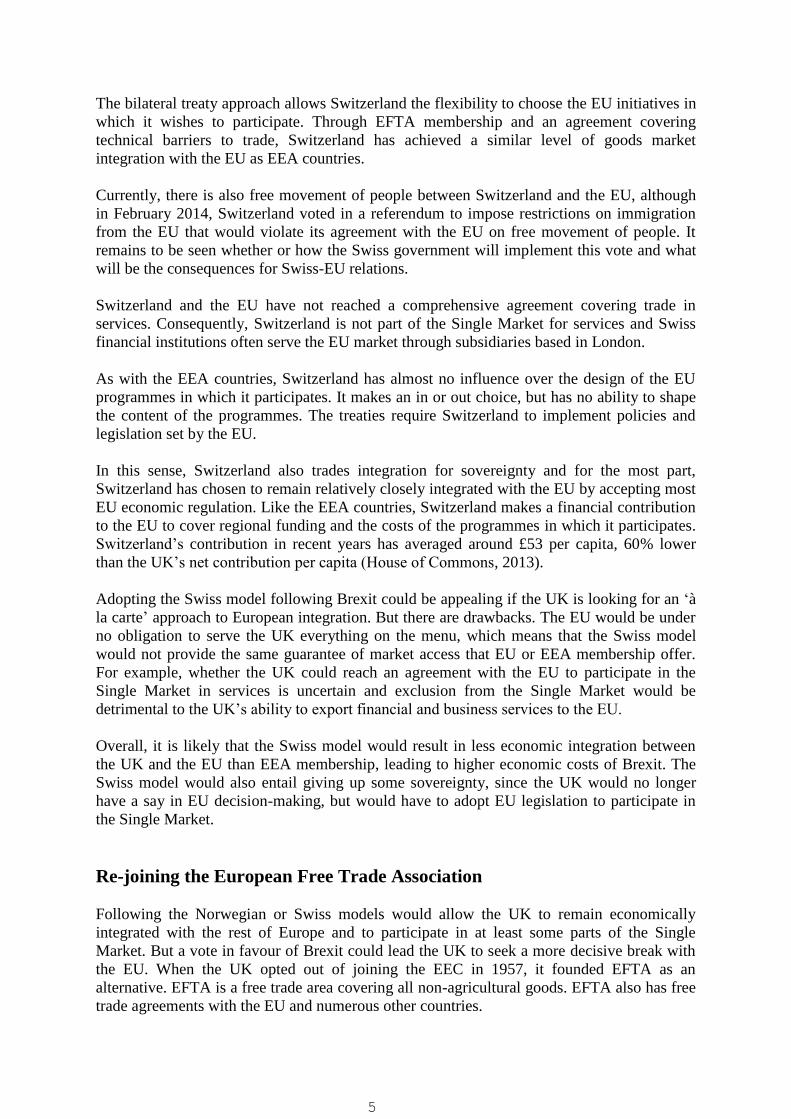
The bilateral treaty approach allows Switzerland the flexibility to choose the EU initiatives in

which it wishes to participate. Through EFTA membership and an agreement covering

technical barriers to trade, Switzerland has achieved a similar level of goods market

integration with the EU as EEA countries.

Currently, there is also free movement of people between Switzerland and the EU, although

in February 2014, Switzerland voted in a referendum to impose restrictions on immigration

from the EU that would violate its agreement with the EU on free movement of people. It

remains to be seen whether or how the Swiss government will implement this vote and what

will be the consequences for Swiss-EU relations.

Switzerland and the EU have not reached a comprehensive agreement covering trade in

services. Consequently, Switzerland is not part of the Single Market for services and Swiss

financial institutions often serve the EU market through subsidiaries based in London.

As with the EEA countries, Switzerland has almost no influence over the design of the EU

programmes in which it participates. It makes an in or out choice, but has no ability to shape

the content of the programmes. The treaties require Switzerland to implement policies and

legislation set by the EU.

In this sense, Switzerland also trades integration for sovereignty and for the most part,

Switzerland has chosen to remain relatively closely integrated with the EU by accepting most

EU economic regulation. Like the EEA countries, Switzerland makes a financial contribution

to the EU to cover regional funding and the costs of the programmes in which it participates.

Switzerland’s contribution in recent years has averaged around £53 per capita, 60% lower

than the UK’s net contribution per capita (House of Commons, 2013).

Adopting the Swiss model following Brexit could be appealing if the UK is looking for an ‘à

la carte’ approach to European integration. But there are drawbacks. The EU would be under

no obligation to serve the UK everything on the menu, which means that the Swiss model

would not provide the same guarantee of market access that EU or EEA membership offer.

For example, whether the UK could reach an agreement with the EU to participate in the

Single Market in services is uncertain and exclusion from the Single Market would be

detrimental to the UK’s ability to export financial and business services to the EU.

Overall, it is likely that the Swiss model would result in less economic integration between

the UK and the EU than EEA membership, leading to higher economic costs of Brexit. The

Swiss model would also entail giving up some sovereignty, since the UK would no longer

have a say in EU decision-making, but would have to adopt EU legislation to participate in

the Single Market.

Re-joining the European Free Trade Association

Following the Norwegian or Swiss models would allow the UK to remain economically

integrated with the rest of Europe and to participate in at least some parts of the Single

Market. But a vote in favour of Brexit could lead the UK to seek a more decisive break with

the EU. When the UK opted out of joining the EEC in 1957, it founded EFTA as an

alternative. EFTA is a free trade area covering all non-agricultural goods. EFTA also has free

trade agreements with the EU and numerous other countries.

5

Re-joining EFTA would guarantee UK goods tariff-free access to the EU and ensure the UK

did not impose tariffs on goods imported from the EU. But it would not provide for free

movement of people or free trade in services between the UK and the EU. Since the UK

would not belong to the Single Market, re-joining EFTA would also probably result in a

gradual divergence between economic regulation in the UK and the EU. This would increase

‘non-tariff barriers’ to trade between the UK and the EU.3

Ottaviano et al (2014) estimate the costs of Brexit to the UK economy would come primarily

from increases in non-tariff barriers between the UK and the EU, not from changes in tariffs.

This suggests there would be an economic price to pay for joining EFTA.

In 1960, when EFTA came into being, reducing tariffs was the primary goal of efforts to

lower trade costs and promote international economic integration. But the success of the

World Trade Organization (WTO), the EU and other regional and bilateral trade agreements

in lowering tariffs has shifted the focus of today’s trade negotiations – such as the

Transatlantic Trade and Investment Partnership (TTIP) – towards non-tariff barriers and trade

in services and capital. EFTA is not designed to promote integration in these areas.

Consequently, all EFTA members have either left to join the EU or sought greater integration

with the EU through other channels.

At present, the members of EFTA are Iceland, Liechtenstein, Norway and Switzerland. All

these countries are either members of the EEA (Iceland, Liechtenstein and Norway) or have

their own bilateral agreements with the EU (Switzerland). Unless the UK wishes to opt out of

all forms of economic integration except tariff removal, re-joining EFTA is not a stand-alone

solution to the problem of what should follow Brexit.

World Trade Organization – the fallback option?

Suppose the UK leaves the EU without putting in place any of the alternative arrangements

discussed above. Then the country’s trade with both the EU and almost all the rest of the

world would be governed by the WTO. As of 2015, the WTO has 161 members comprising

all major economies and most minor ones. Under WTO rules, each member must grant the

same ‘most favoured nation’ (MFN) market access, including charging the same tariffs, to all

other WTO members. The only exceptions to this principle are that countries can choose to

enter into free trade agreements such as the EU or EFTA and can give preferential market

access to developing countries.

As a WTO member, the UK’s exports to the EU and other WTO members would be subject

to the importing countries’ MFN tariffs. Compared with EU or EFTA membership, this

would raise the cost of exporting to the EU for UK firms (Ottaviano et al, 2014). The UK’s

services trade would also be subject to WTO rules. Since the WTO has made far less progress

than the EU in liberalising trade in services, this would mean reduced access to EU markets

for UK service producers.

3 ‘Non-tariff barriers’ is a catch-all term referring to any measure that raises the costs of trade but does not take

the form of a tariff. It covers everything from quantitative trade restrictions such as import licensing to border

costs of complying with customs procedures and behind the border costs caused by regulatory or product

standard differences across countries. The EU Single Market has reduced non-tariff barriers between member

states by removing customs procedures and harmonising regulations and product standards.

6

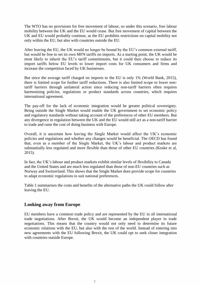
The WTO has no provisions for free movement of labour, so under this scenario, free labour

mobility between the UK and the EU would cease. But free movement of capital between the

UK and EU would probably continue, as the EU prohibits restrictions on capital mobility not

only within the EU, but also with countries outside the EU.

After leaving the EU, the UK would no longer be bound by the EU’s common external tariff,

but would be free to set its own MFN tariffs on imports. As a starting point, the UK would be

most likely to inherit the EU’s tariff commitments, but it could then choose to reduce its

import tariffs below EU levels to lower import costs for UK consumers and firms and

increase the competition faced by UK businesses.

But since the average tariff charged on imports to the EU is only 1% (World Bank, 2015),

there is limited scope for further tariff reductions. There is also limited scope to lower non-

tariff barriers through unilateral action since reducing non-tariff barriers often requires

harmonising policies, regulations or product standards across countries, which requires

international agreement.

The pay-off for the lack of economic integration would be greater political sovereignty.

Being outside the Single Market would enable the UK government to set economic policy

and regulatory standards without taking account of the preferences of other EU members. But

any divergence in regulation between the UK and the EU would still act as a non-tariff barrier

to trade and raise the cost of doing business with Europe.

Overall, it is uncertain how leaving the Single Market would affect the UK’s economic

policies and regulations and whether any changes would be beneficial. The OECD has found

that, even as a member of the Single Market, the UK’s labour and product markets are

substantially less regulated and more flexible than those of other EU countries (Koske et al,

2015).

In fact, the UK’s labour and product markets exhibit similar levels of flexibility to Canada

and the United States and are much less regulated than those of non-EU countries such as

Norway and Switzerland. This shows that the Single Market does provide scope for countries

to adapt economic regulations to suit national preferences.

Table 1 summarises the costs and benefits of the alternative paths the UK could follow after

leaving the EU.

Looking away from Europe

EU members have a common trade policy and are represented by the EU in all international

trade negotiations. After Brexit, the UK would become an independent player in trade

negotiations. This means that the country would not only need to determine its future

economic relations with the EU, but also with the rest of the world. Instead of entering into

new agreements with the EU following Brexit, the UK could opt to seek closer integration

with countries outside Europe.

7

Table 1: Options for the UK outside the EU

Pros Cons

EEA – the Norway model o Belong to the Single Market.

o Able to negotiate trade deals independently of the

EU.

o Required to implement Single Market policies, but

have no representation in setting the rules of the

Single Market.

o Must comply with rules of origin for exports to the

EU and subject to EU anti-dumping measures.

o Must contribute to the EU budget.

Bilateral agreements – the

Swiss model

o Free trade in goods and free movement of people

with the EU.


EU.

o A la carte approach permits opting out of EU

programmes on a case-by-case basis.

o Bilateral agreements require Switzerland to adopt

EU rules, but Swiss have no representation in EU

decision making.

o No agreement with the EU on trade in services.

o Pay a fee to participate in EU programmes, but

contribution likely to be lower than if in EEA.

EFTA o Free trade in goods with the EU.


EU.

o Not required to adopt EU economic policies and

regulations.

o No obligation to contribute to the EU budget.

o No freedom of movement of people with the EU.

o No right of access to EU markets for service

providers.

o Goods exported to the EU must meet EU product

standards.

WTO o Able to negotiate trade deals independently of the

EU.

o Not required to adopt EU economic policies and

regulations.

o No obligation to contribute to the EU budget.

o Trade with EU subject to MFN tariffs and any non-

tariff barriers that comply with WTO agreements.

o No freedom of movement of people with the EU.

o No right of access to EU markets for service

providers.

o Goods exported to the EU must meet EU product

standards.

8

For example, the UK could propose a free trade area among Commonwealth countries or

could attempt to join Canada, Mexico and the United States as a member of the North

American Free Trade Agreement (NAFTA). Of course, the EU is also working to dismantle

trade barriers with the rest of the world, such as through the TTIP agreement currently being

negotiated with the United States. It is uncertain whether leaving the EU would enable the

UK to negotiate more and better trade agreements than it can as part of the EU.

Even without the UK, the EU is the world's second largest exporter behind China and the

world's second largest importer behind the United States. This makes the EU a desirable trade

partner and gives the EU an important voice in trade negotiations. Since the UK is a much

smaller market than the EU, the country alone would have less bargaining power in

international trade negotiations than the EU currently has.

On the other hand, Brexit would enable the UK to seek trade agreements tailored to the

interests of UK businesses and consumers rather than having to make compromises to meet

the needs of other EU countries.

Whether the benefits from greater autonomy in trade negotiations would outweigh the costs

from reduced bargaining power is hard to predict, but some insight into how the UK may fare

following Brexit can be gained by looking at the experience of Canada – another medium-

sized developed economy in close proximity to a much larger market.

Under NAFTA, there is free trade between Canada, Mexico and the United States, but one of

the costs of obtaining access to the US market is adoption of the provisions of the ‘investment

state dispute settlement’ (ISDS). ISDS clauses are almost always included in US trade

agreements (Poulsen et al, 2013) and they allow US investors to bring claims directly against

the Canadian government (and vice versa). By contrast, under the WTO’s dispute settlement

mechanism, investors must go through their home government to bring a claim against

another country.

Cases brought against Canada under the ISDS have covered issues such as the decision to

introduce plain packaging of tobacco products and ‘anti-graft’ rules that would restrict

companies convicted of corruption from receiving government contracts. This has raised

concerns that ISDS clauses provide too much protection to foreign investors and effectively

curtail national sovereignty.

There is also evidence that US firms are better able to take advantage of ISDS provisions than

Canadian firms. The United States has won all of the 11 decided cases that it has initiated

under the ISDS, while Canada has won seven of its 13 decided cases (CCPA, 2015).

The scope of ISDS provisions is a key point of contention in the TTIP negotiations between

the United States and the EU. The EU has sufficient bargaining power to push back against

rules designed to advance the interests of US firms. It is unlikely that the UK alone would

have similar leverage.

Reducing trade barriers between the UK and the rest of the world is a laudable aim and would

be likely to increase trade and raise UK income. But it is not an adequate replacement for EU

membership. The best-known fact in international economics is that international trade and

investment fall substantially with distance (Head and Mayer, 2014). Doubling the distance

between two countries roughly halves the trade between them. The UK is much closer

9

geographically to the EU than to other large economies such as the United States or China

and, therefore, it is not surprising that roughly half of the UK’s trade is with the EU

(Ottaviano et al, 2014).

Put another way, it is geography rather than policy that makes the EU the UK’s most

important economic partner. Simply reorienting the focus of the UK’s trade policy away from

Europe will not change this underlying reality. Whatever agreements are reached with

countries outside Europe, the most important decision facing the government following

Brexit would still be the future of the UK’s relations with the EU.

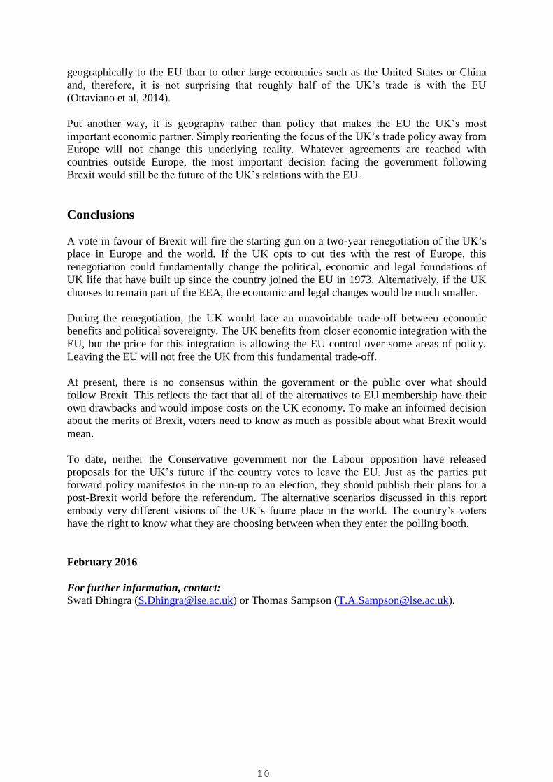
Conclusions

A vote in favour of Brexit will fire the starting gun on a two-year renegotiation of the UK’s

place in Europe and the world. If the UK opts to cut ties with the rest of Europe, this

renegotiation could fundamentally change the political, economic and legal foundations of

UK life that have built up since the country joined the EU in 1973. Alternatively, if the UK

chooses to remain part of the EEA, the economic and legal changes would be much smaller.

During the renegotiation, the UK would face an unavoidable trade-off between economic

benefits and political sovereignty. The UK benefits from closer economic integration with the

EU, but the price for this integration is allowing the EU control over some areas of policy.

Leaving the EU will not free the UK from this fundamental trade-off.

At present, there is no consensus within the government or the public over what should

follow Brexit. This reflects the fact that all of the alternatives to EU membership have their

own drawbacks and would impose costs on the UK economy. To make an informed decision

about the merits of Brexit, voters need to know as much as possible about what Brexit would

mean.

To date, neither the Conservative government nor the Labour opposition have released

proposals for the UK’s future if the country votes to leave the EU. Just as the parties put

forward policy manifestos in the run-up to an election, they should publish their plans for a

post-Brexit world before the referendum. The alternative scenarios discussed in this report

embody very different visions of the UK’s future place in the world. The country’s voters

have the right to know what they are choosing between when they enter the polling booth.

February 2016

For further information, contact:

Swati Dhingra ([email protected]) or Thomas Sampson ([email protected]).

10



Further reading

Cameron, D. (2013) ‘EU Speech at Bloomberg’, 23 January 2013. Retrieved from:

https://www.gov.uk/government/speeches/eu-speech-at-bloomberg

Campos, N., F. Coricelli and L. Moretti. (2015) ‘Norwegian Rhapsody? The Political

Economy Benefits of Regional Integration’, CEPR Discussion Paper 10653.

CCPA (2015) ‘NAFTA Chapter 11 Investor-State Disputes’, 14 January 2015, Canadian

Centre for Policy Alternatives.

Head, K. and T. Mayer (2014) ‘Gravity Equations: Workhorse, Toolkit, Cookbook’,

Handbook of International Economics Vol. 4.

House of Commons (2013) ‘Leaving the EU’, Research Paper 13/42, 1 July 2013.

Koske, I., I. Wanner, R. Bitetti and O. Barbiero (2015) ‘The 2013 Update of the OECD

Product Market Regulation Indicators: Policy Insights for OECD and Non-OECD Countries’,

OECD Economics Department Working Papers, 1200/2015.

Ottaviano, G., J. P. Pessoa, T. Sampson and J. Van Reenen (2014) ‘The Costs and Benefits of

Leaving the EU’, Centre for Economic Performance Policy Analysis

http://cep.lse.ac.uk/pubs/download/pa016.pdf

Parker, G. (2015). ‘Tories Shun Brexit Contingency Plans’, Financial Times, 1 December

2015. Retrieved from: http://www.ft.com/cms/s/0/208fdf8c-9846-11e5-95c7-

d47aa298f769.html#axzz3xSEYNfkq

Philippidis, G. and L. J. Hubbard (2001) ‘The Economic Cost of the CAP Revisited’,

Agricultural Economics, 25, 375-385.

Poulsen, L., J. Bonnitcha and J. Yackee (2013) ‘Costs and Benefits of an EU-USA

Investment Protection Treaty’, LSE Enterprise Report to the BIS, April 2013.

Stewart-Brown, R. and F. Bungay (2012) ‘Rules of Origin in EU Free Trade Agreements’,

Trade Policy Centre Research Paper.

Ugwumadu, J. (2013) ‘Poland Takes Lion’s Share of EU Funds’, Public Finance

International, 28 November 2013. Retrieved from:

http://www.publicfinanceinternational.org/news/2013/11/poland-takes-lion%E2%80%99s-

share-eu-funds

World Bank (2015) ‘World Development Indicators’.

11

https://www.gov.uk/government/speeches/eu-speech-at-bloomberg

http://cep.lse.ac.uk/pubs/download/pa016.pdf

http://www.ft.com/cms/s/0/208fdf8c-9846-11e5-95c7-d47aa298f769.html#axzz3xSEYNfkq

http://www.ft.com/cms/s/0/208fdf8c-9846-11e5-95c7-d47aa298f769.html#axzz3xSEYNfkq

http://www.publicfinanceinternational.org/news/2013/11/poland-takes-lion%E2%80%99s-share-eu-funds

http://www.publicfinanceinternational.org/news/2013/11/poland-takes-lion%E2%80%99s-share-eu-funds

The consequences of Brexit for UK trade and living standards


#CE

PB

RE

XIT

BR

EXITP

AP

ER

Introduction

The outcome of the UK’s referendum on membership of the European Union (EU) will shape

the future of the country’s relationship with its largest trade partner – the EU. Membership of

the EU has reduced trade costs between the UK and the rest of Europe. Most obviously, there

is a customs union between EU members, which means that all tariff barriers have been

removed within the EU, allowing for free trade in goods and services.

But equally important in reducing trade costs has been the reduction of non-tariff barriers

resulting from the EU’s continuing efforts to create a ‘single market’ within Europe.1 Non-

tariff barriers include a wide range of measures that raise the costs of trade such as border

controls, rules of origin checks, cross-country differences in regulations over things like

product standards and safety, and threats of anti-dumping.

Reductions in trade barriers have increased trade between the UK and the EU. Prior to the

UK joining the European Economic Community (EEC) in 1973, around one third of UK

trade was with the EEC. In 2014, the 27 other EU members accounted for 45% of the UK’s

exports and 53% of our imports (ONS, 2015). EU exports comprise 13% of UK national

income.

Higher trade benefits UK consumers through lower prices and access to better goods and

services. At the same time, the UK’s workers and businesses benefit from new export

opportunities that lead to higher sales and profits and allow the UK to specialise in industries

in which it has a comparative advantage. Through these channels, increased trade raises

output, incomes and living standards in the UK.

These standard ‘static’ effects of trade have been understood for many centuries since at least

the work of David Ricardo. But in recent decades, studies of trade have revealed very large

effects on wellbeing through other routes such as higher productivity and innovation.

How would Brexit affect the UK’s trade, and what impact would this have on incomes in the

UK? This briefing reports new estimates of how Brexit would affect UK living standards

through trade (updating our earlier analysis in Ottaviano et al, 2014). We report a range of

forecasts based on alternative estimation methods and different assumptions about how the

UK’s relationship with the EU would change following Brexit. We primarily focus on the

narrow, static trade consequences of Brexit rather than other channels through which Brexit

could affect the UK’s economy, such as investment or migration.

Although it is always hard to assess what the economic future may bring and there are many

uncertainties, we consistently find that by reducing trade, Brexit would lower UK living

standards. Importantly, the fall in income per capita resulting from lower trade more than

offsets any savings that the UK obtains from reduced fiscal contributions to the EU budget.

Our baseline estimates imply that, after accounting for fiscal savings, the effect of Brexit is

equivalent to a fall in UK income of between 1.3% and 2.6% – that is, a decline in average

annual household income of between £850 and £1,700 per year.

1 The single market is the name given to the integrated European economy created by removing economic

barriers between EU members.

13

Our baseline estimates come from a state-of-the-art static model of the global economy. We

also present estimates using empirical evidence on the links between EU membership, trade

and income. This ‘reduced-form’ approach captures the long-run effects of leaving the EU on

productivity growth and leads to much higher estimates. In this case, we calculate that Brexit

may reduce national income by between 6.3% and 9.5% – that is, about £4,200 to £6,400 per

household per year.

We abstract away from the cost of the policy uncertainty that will result from the negotiations

over Brexit. The impact of such uncertainty has been found to be important in much recent

research (Handley and Limão, 2015).

Estimating the effects of Brexit

To estimate the effect of Brexit on the UK’s trade and living standards, we use a modern

quantitative trade model of the global economy. Quantitative trade models incorporate the

channels through which trade affects consumers, firms and workers, and provide a mapping

from trade data to welfare. The model provides numbers for how much real incomes change

under different trade policies, using readily available data on trade volumes and potential

trade barriers. Our model uses the most recent data (WIOD) which divides the world into 35

sectors and 31 regions. It allows for trade in both intermediate inputs and final output in both

goods and services. The model takes into account the effects of Brexit on the UK’s trade with

the EU and the UK’s trade with the rest of the world.

To forecast the consequences of the UK leaving the EU, we must make assumptions about

how trade costs change following Brexit. It is not known exactly how the UK’s relations with

the EU would change following Brexit, which means that there is a lack of clarity over the

consequences of Brexit for trade costs between the UK and the EU.

To overcome this difficulty, we analyse two scenarios: an optimistic scenario in which the

increase in trade costs between the UK and the EU is small, and; a pessimistic scenario with a

larger rise in trade costs.

The optimistic scenario assumes that in a post-Brexit world, the UK’s trade relations with the

EU are similar to those currently enjoyed by Norway. As a member of the European

Economic Area (EEA), Norway has a free trade agreement with the EU, which means that

there are no tariffs on trade between Norway and the EU. Norway is also a member of the

European single market and adopts policies and regulations designed to reduce non-tariff

barriers within the single market.

But Norway is not a member of the EU’s customs union, so it faces some non-tariff barriers

that do not apply to EU members such as rules of origin requirements and anti-dumping

duties. Campos et al (2015) find that Norway’s productivity growth has been harmed by not

fully participating in the EU’s market integration programmes.

In the pessimistic scenario, we assume that the UK is not successful in negotiating a new

trade agreement with the EU and, therefore, that trade between the UK and the EU following

Brexit is governed by World Trade Organisation (WTO) rules. This implies larger increases

14

in trade costs than the optimistic scenario because most favoured nation (MFN) tariffs2 are

imposed on UK-EU trade and because the WTO has made less progress on reducing non-

tariff barriers than the EU.

Increases in trade costs between the UK and the EU following Brexit can be divided into

three parts: (i) higher tariffs on imports; (ii) higher non-tariff barriers to trade (arising from

different regulations, border controls, etc.); and (iii) the UK may not participate in future

steps that the EU takes towards deeper integration and the reduction of non-tariff barriers

within the EU.

In the optimistic scenario, we assume that the UK and the EU continue to enjoy a free trade

agreement and Brexit does not lead to any change in tariff barriers. In the pessimistic scenario

where trade is governed by WTO rules, we assume MFN tariffs are imposed on UK-EU

goods trade.

Regarding non-tariff barriers, in the optimistic scenario, we assume that UK-EU trade is

subject to one quarter of the reducible non-tariff barriers that are observed in trade between

the United States and the EU. In the pessimistic scenario, we assume a larger increase of

three quarters of reducible non-tariff barriers.3

Finally, trade costs between countries within the EU have been declining approximately 40%

faster than trade costs between other OECD countries (Méjean and Schwellnus, 2009). In the

event of Brexit, the UK would not benefit from any future reductions in intra-EU trade costs.

In the optimistic scenario, we assume that in the ten years following Brexit, intra-EU trade

costs fall 20% faster than in the rest of the world, while in the pessimistic scenario, we

assume intra-EU trade costs continue to fall 40% faster than in the rest of the world. This

implies that in the optimistic case, non-tariff barriers within the EU fall 5.7% over the next

decade, while in the pessimistic case they fall by 12.8%.4

Our estimates also account for fiscal transfers between the UK and the EU. Like all EU

members, the UK makes a contribution to the EU budget. The net fiscal contribution of the

UK to the EU budget has been estimated to be around 0.53% of national income (HM

Treasury, 2013). One benefit of Brexit for the UK would be a reduced contribution to the EU

budget.

But Brexit would not necessarily mean that the UK would make zero contribution to the EU

budget. In return for access to the single market, EEA members such as Norway make

substantial payments to the EU. On a per capita basis, Norway’s financial contribution to the

EU is 83% as large as the UK’s payment (House of Commons, 2013). Therefore, in the

optimistic case we assume that the UK’s contribution to the EU budget falls by 17% (that is,

0.09% of national income).

2 Under WTO rules, each member must grant the same ‘most favoured nation’ (MFN) market access, including

charging the same tariffs, to all other WTO members. The only exceptions to this principle are that countries can

choose to enter into free trade agreements such as the EU or the European Free Trade Association and can give

preferential market access to developing countries. 3 These assumptions imply a non-tariff barrier increase of 2.0% in the optimistic scenario and 6.0% in the

pessimistic scenario. Our data on non-tariff barriers between the United States and the EU are taken from

Berden et al (2009, 2013). 4 See Dhingra et al (2016) for a complete explanation of how these changes are calculated.

15

In the pessimistic case where the UK is outside the EEA, we assume that the UK saves more

of its current contribution. The 0.53% saving includes only the public finance components so

excludes all the transfers the EU makes directly to universities, firms and other non-

governmental bodies. Under the reasonable assumption that post-Brexit the UK government

does not cut this funding, the saving is 0.31% according to Eurostat

(http://ec.europa.eu/budget/figures/2007-2013/index_en.cfm).5 This cost essentially comes

from the agricultural subsidies in the Common Agricultural Policy.

Table 1 summarises the results of our analysis. For each case, we calculate the percentage

change in the level of income per capita that has the same effect on living standards in the

UK as Brexit.6 The numbers we report should be interpreted as permanent changes in average

income per capita in the UK that occur immediately following Brexit.

In the optimistic scenario, there is an overall fall in income of 1.28% that is largely driven by

current and future changes in non-tariff barriers. Non-tariff barriers play a particularly

important role in restricting trade in services, an area where the UK is a major exporter. In the

pessimistic scenario, the overall loss increases to 2.61%.

The costs of reduced trade far outweigh the fiscal savings in both scenarios. In cash terms, the

cost of Brexit to the average UK household is £850 per year in the optimistic scenario and

£1,700 per year in the pessimistic scenario.

Table 1: The effects of Brexit on UK living standards

Optimistic Pessimistic

Trade effects -1.37% -2.92%

Fiscal benefit 0.09% 0.31%

Total change in income per capita -1.28% -2.61%

Income change per household -£850 -£1,700

Source: CEP calculations (see Dhingra et al, 2016, for technical details).

Notes: Optimistic scenario: Increase in EU/UK Non-Tariff Barriers (+2%) + exclusion from future fall in NTB

within EU (-5.7%), saving of 17% of 0.53% lower fiscal transfer. Pessimistic scenario: MFN Tariff + increase

in EU/UK Non-Tariff Barriers (+6%) + exclusion from future fall in NTB within EU (-12.8%), saving of 0.31%

net fiscal transfer.

The effect of Brexit on other countries

Although we have focused on the UK, the fall in trade also affects other countries. Figure 1

shows the distribution of changes in income per capita across countries in the optimistic and

pessimistic scenarios. All EU members are worse off: Ireland suffers the largest proportional

losses from Brexit, alongside the Netherlands and Belgium. Countries that lose the most are

those currently trading the most with the UK. Some countries outside the EU, such as Russia

and Turkey, gain as trade is diverted towards them and away from the EU.

5 Note that we are overstating the benefits of Brexit in the optimistic scenario by using the higher 0.53%

number. But we do not have accurate calculations on the comparable fraction of the 0.31% net fiscal

contribution for Norway. 6 Formally, we calculate the permanent percentage change in income per capita that has the same present

discounted value effect on welfare in the UK as Brexit. We assume an annual discount rate of 4% and an

intertemporal elasticity of substitution equal to one.

16

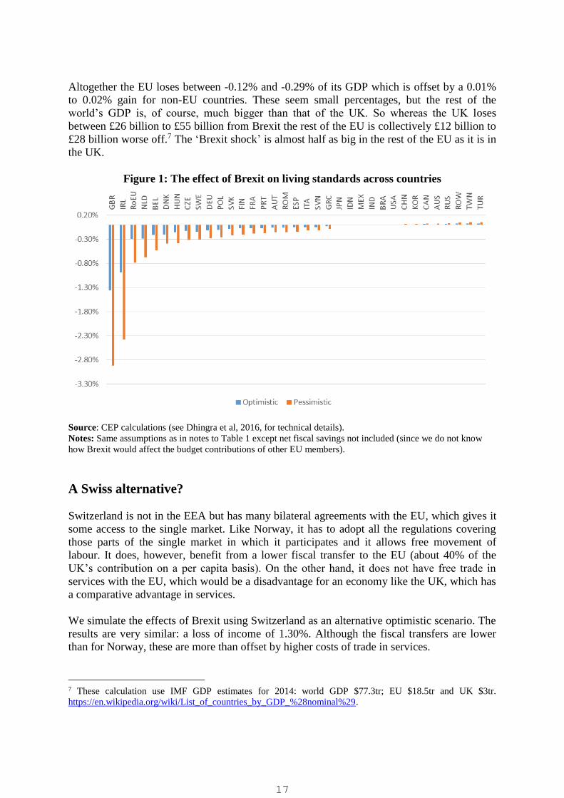
http://ec.europa.eu/budget/figures/2007-2013/index_en.cfm

Altogether the EU loses between -0.12% and -0.29% of its GDP which is offset by a 0.01%

to 0.02% gain for non-EU countries. These seem small percentages, but the rest of the

world’s GDP is, of course, much bigger than that of the UK. So whereas the UK loses

between £26 billion to £55 billion from Brexit the rest of the EU is collectively £12 billion to

£28 billion worse off.7 The ‘Brexit shock’ is almost half as big in the rest of the EU as it is in

the UK.

Figure 1: The effect of Brexit on living standards across countries


Notes: Same assumptions as in notes to Table 1 except net fiscal savings not included (since we do not know

how Brexit would affect the budget contributions of other EU members).

A Swiss alternative?

Switzerland is not in the EEA but has many bilateral agreements with the EU, which gives it

some access to the single market. Like Norway, it has to adopt all the regulations covering

those parts of the single market in which it participates and it allows free movement of

labour. It does, however, benefit from a lower fiscal transfer to the EU (about 40% of the

UK’s contribution on a per capita basis). On the other hand, it does not have free trade in

services with the EU, which would be a disadvantage for an economy like the UK, which has

a comparative advantage in services.

We simulate the effects of Brexit using Switzerland as an alternative optimistic scenario. The

results are very similar: a loss of income of 1.30%. Although the fiscal transfers are lower

than for Norway, these are more than offset by higher costs of trade in services.

7 These calculation use IMF GDP estimates for 2014: world GDP $77.3tr; EU $18.5tr and UK $3tr.

https://en.wikipedia.org/wiki/List_of_countries_by_GDP_%28nominal%29.

17

https://en.wikipedia.org/wiki/List_of_countries_by_GDP_(nominal)

Unilateral liberalisation after Brexit?

Following Brexit, the UK would no longer be bound by the EU’s common external tariff on

imports. Proponents of leaving the EU argue the UK could benefit from this change by

unilaterally removing all tariffs on imports into the UK in order to lower the cost of imported

goods. To analyse the consequences of this unilateral liberalisation policy, we re-run our

optimistic and pessimistic scenarios after including the additional assumption that the UK

removes all tariffs on imports from anywhere in the world.

Table 2 reports the results. We find that unilateral liberalisation reduces the costs of Brexit by

0.3 percentage points in both scenarios. But the overall effect of Brexit is still negative. The

reason that the benefits of such a radical move are small is simple. WTO tariffs are already

low, so further reductions do not make much difference. In today’s world, integration is not a

matter of lowering tariff rates. It requires policies, such as hammering out regulatory

differences in services provision that rely on international agreement and cannot be achieved

unilaterally.

Table 2: The effects of Brexit and unilateral trade liberalisation on UK living standards

Optimistic Pessimistic

Brexit trade effects (from Table 1) -1.37% -2.92%

Fiscal benefit (from Table 1) 0.09% 0.31%

Unilateral liberalisation 0.30% 0.32%

Total change in income per capita -0.98% -2.29%


Notes: This includes simulating the unilateral removal of all tariffs on imports into the UK.

Long-run effects of Brexit

The estimates in Table 1 are based on a static trade model that does not account for the

dynamic effects of trade on productivity. Trade can have positive effects through increasing

competition, which reduces excess profits and promotes efficiency. Competition, access to

superior intermediate goods and a larger export market can also stimulate innovation. Recent

research finds that dynamic effects may double or triple the size of the static effects reported

in Table 1 (Bloom et al, 2014; Sampson, 2016).

An alternative way to evaluate the consequences of Brexit is to use the results of reduced-

form empirical studies of the effects of EU membership. Baier et al (2008) find that after

controlling for other determinants of bilateral trade, EU members trade substantially more

with other EU countries than they do with members of the EEA or EFTA. Their estimates

imply that, if the UK leaves the EU and joins EFTA, its trade with countries in the EU will

fall by about a quarter.

Combining this with estimates that a 1% decline in trade reduces income per capita by

between 0.5% and 0.75% (Feyrer, 2009) implies that leaving the EU and joining EEA would

reduce UK income per capita by between 6.3% and 9.5% (£4,200 to £6,400 per household

per year). These estimates are much higher than the costs obtained from the static trade

model, suggesting that the dynamic gains from trade may be important.

18

Interestingly, these larger long-run effects are in the same ballpark as the benefits that the UK

has gained since 1973 from being part of the EU. In a recent survey of the evidence of the

impact of EU membership, Crafts (2016) concludes that EU membership raised UK GDP per

capita by between 8.6% and 10.6%. Economists under-estimated the benefits from EU

membership because they focused on static trade models of the kind we have employed in

Table 1.

The bottom line is that the costs of Brexit could easily be about three times larger than those

in the static analysis shown in Table 1.

Future trade agreements

EU members have a common trade policy and are represented by the EU in all international

trade negotiations. After Brexit, the UK would become an independent player, free to seek its

own trade deals with the rest of the world. The UK could use this freedom to look for new

trade deals with countries such as China, India and the United States.

Our model shows that trade with such non-EU countries does indeed rise after Brexit. But the

magnitude of these increases is not enough to offset the decline in trade with the EU. Being

part of the EU does not restrict UK companies’ ability to trade with the rest of the world, but

as our nearest neighbour and the world’s largest market, the EU is the UK’s natural trade

partner.

When negotiating post-Brexit trade deals, the UK would not need to compromise with other

EU countries. On the other hand, the UK would have to take on the cost of hiring civil

servants to rebuild its capacity to undertake trade negotiations. More importantly, since the

UK is a smaller market than the EU, it would have less bargaining power in trade

negotiations than the EU does.

Has the UK benefited from past trade deals reached by the EU? CEP research by Breinlich et

al (2016) estimates that trade agreements negotiated by the EU over the past two decades

have reduced the quality-adjusted prices of imports into the UK by over one-third. Although

it is often argued that the EU does not pursue trade agreements that are beneficial to the UK,

these consumer benefits are twice as big as those enjoyed by the 12 other members that

joined before 1995.

The EU is currently negotiating a major new free trade agreement with the United States (the

Transatlantic Trade and Investment Partnership or TTIP) – as well as an ‘economic

partnership agreement’ with Japan. If the UK leaves the EU, it will not benefit from these.

Breinlich et al (2016) estimate that the US and Japanese agreements would lower prices by

0.4% and 0.2% respectively. The United States has stated that it would not do a trade deal

with the UK alone (Holehouse, 2015).

Other Brexit effects on migration, foreign investment and regulation

We have focused on the impact of Brexit on UK households through trade. Brexit could also

affect the UK economy through changes in investment, migration and regulation. We will

19

examine these channels more closely in future reports, but one way of interpreting our

findings is that for Brexit to have an economic benefit, these channels must have a

sufficiently large positive effect on the UK economy to outweigh the negative effects we

identify. This is extremely unlikely to be the case.

Brexit is likely to reduce foreign investment, which has been found to lead to higher

productivity – for example, Haskel et al (2002). Pain and Young (2004) estimate that EU

membership adds 2.25% to UK GDP via the channel of foreign direct investment. Similarly,

migration is found to aid growth and help to reduce the budget deficit without serious adverse

labour market effects (Wadsworth, 2015).

Eurosceptics often point to the promise of better and less regulation as a big benefit after

Brexit (for example, Minford, 2015). It is important to realise that regulation will not much

affect the optimistic scenario. This is because to access the single market, countries like

Norway or Switzerland must adopt the same regulations as the rest of the EU (without having

a vote on what these regulations are).

The UK could weaken social, employment and environmental regulation to some degree. But

even if this were politically possible, the UK already has one of the most flexible

employment and product market regulations in the world according to the OECD (second in

product regulation to the United States and third to the United States and Canada in labour

regulations). Even if the GDP impact of such regulations were large (a point on which there

is controversy), further weakening protection to say US levels would make little economic

difference.

If the UK were to accept higher trade costs by giving up high levels of access to EU markets

(the ‘pessimistic scenario’ above), there would be more scope for regulatory loosening. Booth

et al (2015) identify 56 regulations derived from EU legislation where the UK government’s

Impact Assessment finds that the costs outweigh the benefits. Crafts (2016) calculates the

cost of these regulations is 0.9% of the UK’s GDP.

But many of these regulations implement policies that the UK government is committed to

following inside or outside the EU. For example, half of the total cost comes from just two

policies: the Renewable Energy Strategy; and the Working Time Directive. Scrapping these

regulations would mean abandoning the UK’s renewable energy targets and removing rights

such as the entitlement to 20 days paid annual leave.

Even if the regulatory costs of EU membership were 0.9% of GDP, this figure is still less

than half as large as our estimates of the net cost of Brexit even in the purely static case, and

a lot less than the 6.3% to 9.5% costs under the dynamic case. There are many costs of

regulation in the UK, such as our inefficient planning system (as explained, for example, by

the LSE Growth Commission, 2013). But these problems are primarily home-grown, rather

than imports from Brussels.

Conclusions

The economic consequences of leaving the EU will depend on what policies the UK adopts

following Brexit. But lower trade due to reduced integration with EU countries is likely to

cost the UK economy far more than is gained from lower contributions to the EU budget.

20

Even setting aside foreign investment, migration and the dynamic consequences of reduced

trade, we estimate the effects of Brexit on trade and the UK’s contribution to the EU budget

would be equivalent to a fall in income of between 1.3% and 2.6% (£850 to £1,700 per

household per year). And once we include the long-run effects of Brexit on productivity, the

decline in income increases to between 6.3% and 9.5% (about £4,200 to £6,400 per

household per year).

March 2016

For further information, contact:

Swati Dhingra ([email protected]), Gianmarco Ottaviano ([email protected]),

Thomas Sampson ([email protected]), John Van Reenen ([email protected]) or

Romesh Vaitilingam on 07768-661095 ([email protected]).

21






Further reading

Baier, S. L., J. H. Bergstrand, P. Egger and P. A. McLaughlin (2008) ‘Do Economic

Integration Agreements Actually Work? Issues in Understanding the Causes and

Consequences of the Growth of Regionalism’, The World Economy 31(4): 461-97.

Berden, K., J. Francois, S. Tamminen, M. Thelle and P. Wymenga (2009) ‘Non-Tariff

Measures in EU-US Trade and Investment – An Economic Analysis’, Ecorys report prepared

for the European Commission, Reference OJ 2007/S180219493.

Berden, K., J. Francois, K. Tamminen, M. Thelle and P. Wymenga (2013) ‘Non-tariff

Barriers in EU-US Trade and Investment: An Economic Analysis’, Technical Report,

Institute for International and Development Economics.

Bloom, N., P. Romer, S. Terry and J. Van Reenen (2014) ‘A Trapped Factors Model of

Innovation’, Centre for Economic Performance Discussion Paper No. 1261

(http://cep.lse.ac.uk/pubs/download/dp1261.pdf).

Booth, S., C. Howarth, M. Persson, R. Ruparel and P. Swidlicki (2015) ‘What If..? The

Consequences, Challenges and Opportunities facing Britain outside the EU’, London: Open

Europe.

Breinlich, H., S. Dhingra and G. Ottaviano (2016) ‘The Impact of Trade Agreements on

Consumers’, Centre for Economic Performance mimeo.

Campos, N., F. Coricelli and L. Moretti. (2015) ‘Norwegian Rhapsody? The Political

Economy Benefits of Regional Integration’, CEPR Discussion Paper No. 10653.

Crafts, N. (2016) ‘The Growth Effects of EU Membership for the UK: A Review of the

Evidence’, University of Warwick mimeo.

Dhingra, S., H Huang, G Ottaviano, J Pessoa, T Sampson and J Van Reenen (2016) ‘The

Costs and Benefits of Leaving the EU’, Centre for Economic Performance Technical Report.

Feyrer, J. (2009) ‘Trade and Income – Exploiting Time Series in Geography’, NBER

Working Paper No. 14910.

Handley, K. and N. Limão (2015) ‘Trade and Investment under Policy Uncertainty: Theory

and Firm Evidence’, American Economic Journal: Economic Policy 7(4): 189-222.

Haskel, J., S. Pereira and M. Slaughter (2002) ‘Does Inward Foreign Direct Investment Boost

the Productivity of Domestic Firms?’, NBER Working Paper No. 8724.

HM Treasury (2013) ‘European Union Finances 2013’, 19th November.

Holehouse, M. (2015) ‘Major Blow for Brexit Campaign as US Rules Out UK-Only Trade

Deal’, The Telegraph, 29 October 2015

(retrieved from: http://www.telegraph.co.uk/news/worldnews/europe/eu/11962277/Major-

blow-for-Brexit-campaign-as-US-rules-out-UK-only-trade-deal.html).

22

http://cep.lse.ac.uk/pubs/download/dp1261.pdf

http://www.telegraph.co.uk/news/worldnews/europe/eu/11962277/Major-blow-for-Brexit-campaign-as-US-rules-out-UK-only-trade-deal.html

http://www.telegraph.co.uk/news/worldnews/europe/eu/11962277/Major-blow-for-Brexit-campaign-as-US-rules-out-UK-only-trade-deal.html

House of Commons (2013) ‘Leaving the EU’, Research Paper 13/42, 1st July.

LSE Growth Commission (2013) ‘Investing for Prosperity’

(http://www.lse.ac.uk/researchAndExpertise/units/growthCommission/documents/pdf/LSEG

C-Report.pdf).

Méjean, I. and S. Schwellnus (2009) ‘Price Convergence in the European Union: Within

Firms or Composition of Firms?’, Journal of International Economics 78(1): 1-10.

Minford, P. (2015) ‘Evaluating European Trading Arrangements’, Cardiff Economics

Working Paper No. E2015/17.

ONS (2015) ‘How Important is the European Union to UK Trade and Investment?’, Office

for National Statistics, 26 June.

Ottaviano, G., J. Pessoa, T. Sampson and J. Van Reenen (2014) ‘The Costs and Benefits of

Leaving the EU’, Centre for Economic Performance Policy Analysis.

Pain, N. and G. Young (2004) ‘The Macroeconomic Effect of UK Withdrawal from the EU’,

Economic Modelling 21: 387-408.

Sampson, T. (2016) ‘Dynamic Selection: An Idea Flows Theory of Entry, Trade and

Growth’, Quarterly Journal of Economics 131(1): 315-80, 131(1): 315-380.

Wadsworth, J. (2015) ‘Immigration and the UK Labour Market’, Centre for Economic

Performance Election Analysis No. 1 (http://cep.lse.ac.uk/pubs/download/EA019.pdf).

23

http://www.lse.ac.uk/researchAndExpertise/units/growthCommission/documents/pdf/LSEGC-Report.pdf

http://www.lse.ac.uk/researchAndExpertise/units/growthCommission/documents/pdf/LSEGC-Report.pdf

http://cep.lse.ac.uk/pubs/download/EA019.pdf

The impact of Brexit on foreign investment in the UK

Swati Dhingra, Gianmarco Ottaviano, Thomas Sampson andJohn Van Reenen

#CE

PB

RE

XIT

BR

EXITP

AP

ER

Introduction Foreign direct investment (FDI) comprises investments from outside a country to start up new subsidiaries, to expand existing establishments or to acquire local companies. The UK is a major recipient of FDI with an estimated stock value of over £1 trillion, about half of which is from other members of the European Union (EU), according to UK Trade and Investment (UKTI, 2015). Only the United States and China receive more FDI than the UK. Countries generally welcome FDI as it tends to raise productivity, which increases output and wages. FDI brings direct benefits as foreign firms are typically more productive and pay higher wages than domestic firms. But FDI also brings indirect benefits as the new technological and managerial know-how in foreign firms can be adopted by domestic firms, often through multinationals’ supply chain (Harrison and Rodriguez-Clare, 2009). FDI can also increase competitive pressure, which forces managers to improve their performance. There are at least three reasons why FDI might fall if the UK left the EU:

• First, being fully in the Single Market makes the UK an attractive export platform for multinationals as they do not bear potentially large costs from tariff and non-tariff barriers when exporting to the rest of the EU.

• Second, multinationals have complex supply chains and many co-ordination costs

between their headquarters and local branches. These would become more difficult to manage if the UK left the EU. For example, component parts would be subject to different regulations and costs; and intra-firm staff transfers would become more difficult with tougher migration controls.

• Third, uncertainty over the shape of the future trade arrangements between the UK and

the EU would also tend to dampen FDI. This report analyses what could happen to UK FDI inflows after Brexit and what effect these FDI changes could have on income levels in the UK. The effect of EU membership on FDI A number of factors determine where firms choose to locate and invest. Bigger and richer markets tend to attract more firms, which want to be close to their customers. The UK has strong rule of law, flexible labour markets and a highly educated workforce, all of which make it an attractive FDI location whether or not it is in the EU. But since EU membership reduces trade and investment costs, it is likely to have an impact even after controlling for these other factors. To estimate the size of the effect of being in the EU on FDI, we provide a new empirical analysis – see Bruno et al (2016) in the Technical Appendix to this report. It is a statistical model based on the bilateral FDI flows between 34 OECD countries from 1985 to 2013. The model estimates why foreign investors choose to invest in the UK, as opposed to other countries such as Germany, France or the United States. It is similar to the ‘gravity model’ that is the standard way of estimating bilateral flows of exports and imports.

25

Bilateral FDI flows between any pair of countries depend on their respective market size (measured by GDP), the geographical distance between them and other factors such as GDP per capita. The model addresses the question of how much more FDI would flow between two countries if the sender or the recipient joins the EU, once all these factors are taken into account. Since many FDI determinants – such as geographical distance and culture – are broadly stable over time, we can fully control for them by looking only at changes in FDI and its determinants. The data show that there is always a statistically significant positive effect of being in the EU on inward FDI. The magnitude ranges from a 14% to 38% increase in FDI depending on the exact statistical method used with an average of 28% across the main three methods. These estimates are also consistent with those in Campos and Coricelli (2015), who find an impact of 25% to 30% on FDI flows from EU membership using an alternative method comparing the evolution of UK FDI with a set of matched countries as a comparison group. Similarly, Straathof et al (2008) find that EU membership increases inward FDI stocks by 14% from non-EU countries and by 28% from other EU members (using a gravity model but with earlier data). Being a member of the European Free Trade Association (EFTA) like Switzerland does not restore the FDI benefits of being in the EU. In fact, we find no statistical difference between being in EFTA compared with being completely outside the EU like the United States or Japan. So striking a comprehensive free trade deal after Brexit is not a good substitute for full EU membership. By comparison, Baier et al (2008) estimate that EU membership leads to trade with other EU members increasing by a quarter or more (compared with EFTA membership). So the magnitude of the FDI effect on Brexit is in the same ballpark as the effect on overall trade. Since leaving the EU will likely have a smaller proportionate effect than joining, our Technical Appendix concludes that Brexit is likely to reduce FDI inflows to the UK by about 22%.1 How do changes in FDI affect UK incomes? There is much evidence that FDI brings benefits in terms of enhanced productivity. For example, Bloom et al (2012) find that multinationals boost productivity in UK establishments through enhanced technologies and management practices. On top of this direct effect, Haskel et al (2007) find that there are foreign investment ‘spillovers’ to other, UK-owned firms in the same industry. But to get at the nation-wide impact of FDI on output, we need to factor in the many complex ways in which FDI affects people and firms in multiple parts of the economy. This is a tricky task, but fortunately we can draw on the work of Alfaro et al (2004), who estimate the effect of changes in FDI on growth rates across 73 countries. They find that increases in FDI have a large positive impact on GDP growth, especially for countries like the UK that have a highly developed financial sector.

1 Using a baseline estimate of 0.28, we obtain 0.22 = 0.28/(1+0.28). This is very similar to PWC (2016), which finds that UK FDI will be a quarter lower in 2020 because of Brexit.

26

To be very conservative, we assume a scenario where the Brexit-induced fall in FDI lasts only for 10 years and then reverts to its current level. Using the average of the estimates in the Technical Appendix combined with Alfaro et al’s estimates implies a fall in real income of about 3.4% (see the Annex for more detail). Looking at the wider range, we obtain a fall in income of between 1.8% and 4.3%. The magnitude of our FDI effect on income, of 3.4%, is larger than our static estimates of the losses from trade (between 1.3% and 2.6% in Dhingra et al, 2016). The effect of changes in FDI is equivalent to a loss of GDP of around £2,200 per household. Using earlier data, Pain and Young (2004) estimate that EU membership added 2.25% to UK GDP via FDI. As FDI into the UK has grown over time, we find that this channel is becoming more important for income. Such macroeconomic analysis is useful for a bird’s-eye view of the impact of Brexit on national income via lower FDI. Firm-level studies will tend to underestimate the positive impact of FDI as they focus on the productivity of the foreign firm itself or can examine only a limited number of mechanisms for the FDI spillovers (for example, firms who are in the same industry as the multinational or are suppliers or customers). Nevertheless, identifying the causal effects of FDI on economy-wide productivity is intrinsically very difficult and our estimates are subject to considerably more uncertainty than the impact of Brexit on FDI (or trade) itself. So, to obtain a more granular view of the way that key sectors may be affected, we analyse two important UK industries in more detail: cars and financial services. Concentrating on cars Cars are a successful part of UK manufacturing. The UK is now the world’s fourth largest producer and KPMG (2014) argues that ‘much of the recent investment by car manufacturers is in new vehicles which will be predominantly for sale to the EU market.’ In 2014, the car industry contributed around 5.1% to UK exports, and about 40% of its car exports were to the EU.2 In a survey of its members in 2014, the Society for Motor Manufacturers and Traders found that 70% of its members expect Brexit to have a negative medium to long-term impact on their business.3 There are very rich data on the car industry, which enable us to extend the structural gravity model of exports in Dhingra et al (2016) to the decisions of multinationals over where to base their production. Head and Mayer (2015) use information on assembly and sales locations (IHS Automotive data) on 1,775 models across 184 brands. These data include annual flows of each model shipped from 49 assembly countries to 75 destination countries between 2000 and 2013. They also contain information on the headquarters and assembly location of the car. The model accounts for how the headquarters decide where to locate their production – for example, why BMW chooses to produce Minis in the UK when selling to France.

2 http://researchbriefings.files.parliament.uk/documents/SN00611/SN00611.pdf; http://researchbriefings.files.parliament.uk/documents/SN06091/SN06091.pdf. 3 http://www.smmt.co.uk/2014/04/uk-automotive-industry-europe.

27

http://researchbriefings.files.parliament.uk/documents/SN00611/SN00611.pdf

http://researchbriefings.files.parliament.uk/documents/SN06091/SN06091.pdf

http://www.smmt.co.uk/2014/04/uk-automotive-industry-europe

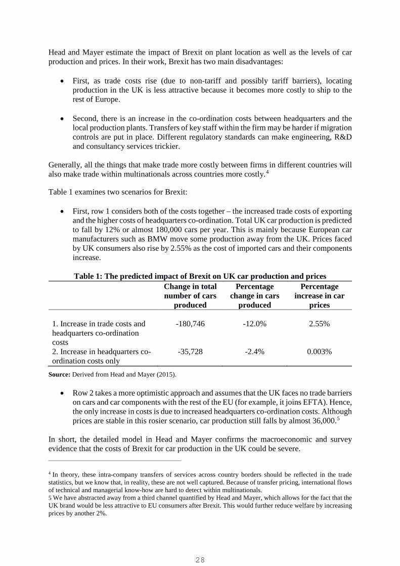
Head and Mayer estimate the impact of Brexit on plant location as well as the levels of car production and prices. In their work, Brexit has two main disadvantages:

• First, as trade costs rise (due to non-tariff and possibly tariff barriers), locating production in the UK is less attractive because it becomes more costly to ship to the rest of Europe.

• Second, there is an increase in the co-ordination costs between headquarters and the

local production plants. Transfers of key staff within the firm may be harder if migration controls are put in place. Different regulatory standards can make engineering, R&D and consultancy services trickier.

Generally, all the things that make trade more costly between firms in different countries will also make trade within multinationals across countries more costly.4

Table 1 examines two scenarios for Brexit:

• First, row 1 considers both of the costs together – the increased trade costs of exporting and the higher costs of headquarters co-ordination. Total UK car production is predicted to fall by 12% or almost 180,000 cars per year. This is mainly because European car manufacturers such as BMW move some production away from the UK. Prices faced by UK consumers also rise by 2.55% as the cost of imported cars and their components increase.

Table 1: The predicted impact of Brexit on UK car production and prices

Change in total number of cars

produced

Percentage change in cars

produced

Percentage increase in car

prices 1. Increase in trade costs and headquarters co-ordination costs

-180,746 -12.0% 2.55%

2. Increase in headquarters co-ordination costs only

-35,728 -2.4% 0.003%

Source: Derived from Head and Mayer (2015).

• Row 2 takes a more optimistic approach and assumes that the UK faces no trade barriers on cars and car components with the rest of the EU (for example, it joins EFTA). Hence, the only increase in costs is due to increased headquarters co-ordination costs. Although prices are stable in this rosier scenario, car production still falls by almost 36,000.5

In short, the detailed model in Head and Mayer confirms the macroeconomic and survey evidence that the costs of Brexit for car production in the UK could be severe.

4 In theory, these intra-company transfers of services across country borders should be reflected in the trade statistics, but we know that, in reality, these are not well captured. Because of transfer pricing, international flows of technical and managerial know-how are hard to detect within multinationals. 5 We have abstracted away from a third channel quantified by Head and Mayer, which allows for the fact that the UK brand would be less attractive to EU consumers after Brexit. This would further reduce welfare by increasing prices by another 2%.

28

Focusing on financial services Financial services have the largest stock of inward FDI in the UK (45%) and constitute 8% of GDP and 12% of tax receipts (Tyler, 2015). The Single Market allows a bank based in one member of the EU to set up a branch or provide cross-border financial services in another, while being regulated by authorities in the home country. This ‘single passport’ to conduct activities in EU member states is important for UK exports of financial services. ‘Passporting’ means that a UK bank can provide services across the EU from its UK home. It also means that a Swiss or an American bank can do the same from a branch or subsidiary established in the UK.6 The UK might be able to negotiate some of these privileges after Brexit. Members of the European Economic Area (EEA) outside the EU (for example, Norway) enjoy them, but they also have to contribute substantially to the EU budget, to accept all EU regulations without a vote on the rules and to allow free labour mobility with the EU. And still for these countries, there seem to be greater difficulties in doing business with the EU (Souta, 2015; Bank of England, 2015). Switzerland is in EFTA (not the EEA) so it enjoys tariff-free access to the EU in goods. But it has no passporting rights, so Swiss financial institutions mostly get access to the EU via special bilateral treaties with the EU, which still require permissions to set up branches in EU members.7 This is one of the reasons that Swiss banks often set up subsidiaries in the UK. The EU's new financial directives have set out further rules for authorisation of the EU operations of Swiss firms, so the Swiss option is unlikely to ensure easy access to EU markets after Brexit (City of London, 2013). More generally, there are concerns that the EEA might not welcome the UK, and that the EU may not grant the special bilateral terms it extended in the past to non-EU countries like Switzerland8, since following Brexit, other cities like Frankfurt and Paris will be keen to grab a larger share of the lucrative markets for financial services.9

Will Brexit relieve the UK financial services sector of onerous EU regulations? It is unlikely to do so because UK-based financial firms would still need to comply with these regulations for all their EU transactions. Another question is whether EU regulations are imposing a big burden on UK firms in their transactions outside the EU. As financial regulations are still evolving, it is difficult to put a monetary value on the impact of Brexit on regulations. But it is unlikely that the regulations put UK firms at a competitive disadvantage as the EU is the world’s largest exporter of financial services, making up a quarter of world financial services exports. Half of the cross-border lending in the world originates within the EU.

6 https://www.dlapiper.com/en/uk/insights/publications/2015/10/banking-disputes-quarterly/brexit/ 7 http://www.bankofengland.co.uk/pra/Pages/authorisations/passporting/faqs.aspx. 8 http://www.publications.parliament.uk/pa/cm201213/cmselect/cmfaff/writev/futunion/m21.pdf; https://www.cityoflondon.gov.uk/business/economic-research-and-information/research-publications/Documents/research-2013/Switzerlands-approach-to-EU-engagement.pdf. 9 http://www.voxeurop.eu/en/content/article/5052502-big-opportunity-europe; http://www.globalcapital.com/article/x1h6hjkpygxb/brexit-casts-long-shadow-over-nervous-uk-banking-sector.

29

https://www.dlapiper.com/en/uk/insights/publications/2015/10/banking-disputes-quarterly/brexit/

http://www.bankofengland.co.uk/pra/Pages/authorisations/passporting/faqs.aspx

http://www.publications.parliament.uk/pa/cm201213/cmselect/cmfaff/writev/futunion/m21.pdf

https://www.cityoflondon.gov.uk/business/economic-research-and-information/research-publications/Documents/research-2013/Switzerlands-approach-to-EU-engagement.pdf

https://www.cityoflondon.gov.uk/business/economic-research-and-information/research-publications/Documents/research-2013/Switzerlands-approach-to-EU-engagement.pdf

http://www.voxeurop.eu/en/content/article/5052502-big-opportunity-europe

http://www.globalcapital.com/article/x1h6hjkpygxb/brexit-casts-long-shadow-over-nervous-uk-banking-sector

The Balance of Competences Review questioned the City of London on the extent to which the Single Market had raised the costs of transacting with countries outside the EU.10 The consensus was that the City became a financial hub while being in the EU, so there was little evidence that membership had seriously hindered the UK’s ability to trade with countries outside the EU. City representatives said that access to the Single Market is one of the major reasons for inward FDI in the UK. Staying in the EU also gives the UK the ability to challenge new regulations at the European Court of Justice, a right that it successfully exercised when the European Central Bank wanted to limit clearing-house activities to the euro area. If the UK leaves the EU, it would lose its leverage in negotiating and challenging future EU regulations. Future trade agreements After Brexit, would the UK strike great deals with non-EU countries that would reduce trade costs and so actually boost FDI? It seems unlikely. Although the UK would no longer need to compromise with other EU countries when negotiating, the UK is under a fifth of the economic size of the EU’s Single Market. It would simply have much less bargaining clout than the EU currently enjoys. Nor would it get automatic access to the new deals struck with the EU, such as those currently being negotiated with Japan and the United States. Conclusions Overall, Brexit is likely to have a negative impact on inward FDI. Our new empirical analysis implies that leaving the EU will reduce FDI inflows to the UK by around 22%. Such losses of investment will damage UK productivity and could lower real incomes by 3.4%. This is larger than our estimates of the static income losses from trade, which are 2.6% even under our ‘pessimistic scenario’ (Dhingra et al, 2016). Case studies of cars and finance also show that Brexit would lower EU-related output of goods and services, and erode the UK’s ability to negotiate concessions from regulations on EU-related transactions. Of course, these costs may be a price that many people are willing to pay to leave the EU. But they are not trivial costs. April 2016 For further information, contact: Swati Dhingra ([email protected]), Thomas Sampson ([email protected]), John Van Reenen ([email protected]), Gianmarco Ottaviano ([email protected]) or Romesh Vaitilingam ([email protected]).

10 https://www.gov.uk/guidance/review-of-the-balance-of-competences.

30





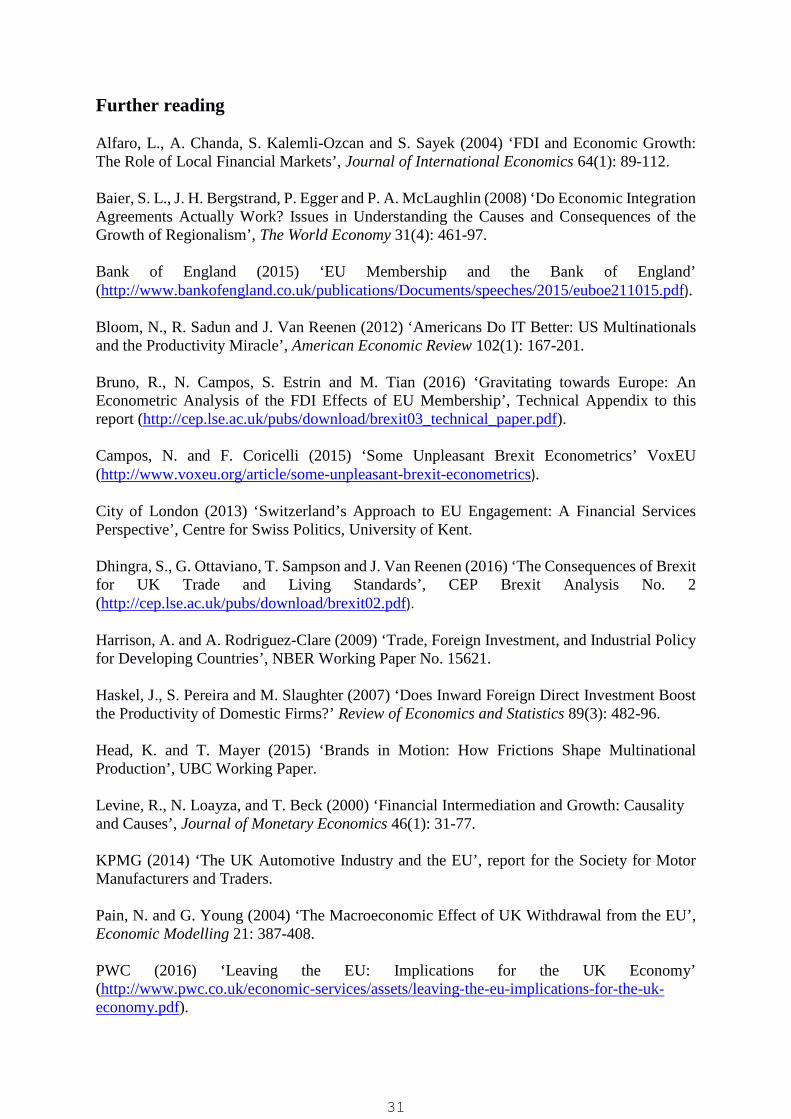
https://www.gov.uk/guidance/review-of-the-balance-of-competences

Further reading Alfaro, L., A. Chanda, S. Kalemli-Ozcan and S. Sayek (2004) ‘FDI and Economic Growth: The Role of Local Financial Markets’, Journal of International Economics 64(1): 89-112. Baier, S. L., J. H. Bergstrand, P. Egger and P. A. McLaughlin (2008) ‘Do Economic Integration Agreements Actually Work? Issues in Understanding the Causes and Consequences of the Growth of Regionalism’, The World Economy 31(4): 461-97. Bank of England (2015) ‘EU Membership and the Bank of England’ (http://www.bankofengland.co.uk/publications/Documents/speeches/2015/euboe211015.pdf). Bloom, N., R. Sadun and J. Van Reenen (2012) ‘Americans Do IT Better: US Multinationals and the Productivity Miracle’, American Economic Review 102(1): 167-201. Bruno, R., N. Campos, S. Estrin and M. Tian (2016) ‘Gravitating towards Europe: An Econometric Analysis of the FDI Effects of EU Membership’, Technical Appendix to this report (http://cep.lse.ac.uk/pubs/download/brexit03_technical_paper.pdf). Campos, N. and F. Coricelli (2015) ‘Some Unpleasant Brexit Econometrics’ VoxEU (http://www.voxeu.org/article/some-unpleasant-brexit-econometrics). City of London (2013) ‘Switzerland’s Approach to EU Engagement: A Financial Services Perspective’, Centre for Swiss Politics, University of Kent. Dhingra, S., G. Ottaviano, T. Sampson and J. Van Reenen (2016) ‘The Consequences of Brexit for UK Trade and Living Standards’, CEP Brexit Analysis No. 2 (http://cep.lse.ac.uk/pubs/download/brexit02.pdf). Harrison, A. and A. Rodriguez-Clare (2009) ‘Trade, Foreign Investment, and Industrial Policy for Developing Countries’, NBER Working Paper No. 15621. Haskel, J., S. Pereira and M. Slaughter (2007) ‘Does Inward Foreign Direct Investment Boost the Productivity of Domestic Firms?’ Review of Economics and Statistics 89(3): 482-96. Head, K. and T. Mayer (2015) ‘Brands in Motion: How Frictions Shape Multinational Production’, UBC Working Paper. Levine, R., N. Loayza, and T. Beck (2000) ‘Financial Intermediation and Growth: Causality and Causes’, Journal of Monetary Economics 46(1): 31-77. KPMG (2014) ‘The UK Automotive Industry and the EU’, report for the Society for Motor Manufacturers and Traders. Pain, N. and G. Young (2004) ‘The Macroeconomic Effect of UK Withdrawal from the EU’, Economic Modelling 21: 387-408. PWC (2016) ‘Leaving the EU: Implications for the UK Economy’ (http://www.pwc.co.uk/economic-services/assets/leaving-the-eu-implications-for-the-uk-economy.pdf).

31

http://www.bankofengland.co.uk/publications/Documents/speeches/2015/euboe211015.pdf

http://cep.lse.ac.uk/pubs/download/brexit03_technical_paper.pdf

http://www.voxeu.org/article/some-unpleasant-brexit-econometrics

http://cep.lse.ac.uk/pubs/download/brexit02.pdf

http://www.pwc.co.uk/economic-services/assets/leaving-the-eu-implications-for-the-uk-economy.pdf


Souta, P. (2015) ‘What Could Brexit Mean for the Financial Services Sector?’ (http://www.britishinfluence.org/what_could_brexit_mean_for_the_financial_services_sector). Straathof, S., G-J. Linders, A. Lejour and J. Mohlmann (2008) ‘The Internal Market and the Dutch Economy: Implications for Trade and Economic Growth’, CPG Netherlands Document No. 168.

Tyler, G. (2015) ‘Financial Services: Contribution to the UK Economy’, Economic Policy and Statistics Section, House of Commons Library, February SN/EP/06193. UKTI (2015) ‘UKTI Inward Investment Report 2014 to 2015’ (https://www.gov.uk/government/publications/ukti-inward-investment-report-2014-to-2015/ukti-inward-investment-report-2014-to-2015-online-viewing).

32

http://www.britishinfluence.org/what_could_brexit_mean_for_the_financial_services_sector

http://econpapers.repec.org/RAS/pli169.htm

http://econpapers.repec.org/RAS/ple145.htm

https://www.gov.uk/government/publications/ukti-inward-investment-report-2014-to-2015/ukti-inward-investment-report-2014-to-2015-online-viewing

https://www.gov.uk/government/publications/ukti-inward-investment-report-2014-to-2015/ukti-inward-investment-report-2014-to-2015-online-viewing

Annex: Calculating the income effects of lower FDI Alfaro et al (2004) estimate a cross-country growth regression with 73 countries to examine the effects of FDI on economic growth. They allow the impact of FDI on GDP growth per capita to vary with the level of development of domestic financial markets. They find that countries with developed financial markets like the UK benefit significantly more from FDI than those with less sophisticated financial systems (like many developing countries). Alfaro et al (2004) present ‘instrumental variables’ (IV) regressions to deal with endogeneity issues. For example, expected growth might affect the level of financial development. We use these more rigorous IV estimates from their Table 7 (column 1), which is based on a regression of average annual per capita growth rate of countries on FDI as a share of GDP, its interaction with financial market development and various controls. The controls include initial GDP, financial market development itself, schooling, population growth, government consumption and a dummy for sub-Saharan Africa, the black market premium, inflation and trade volumes. Since trade volumes are controlled for, the interpretation of the results is the impact of FDI on growth over and above any influence of trade. The financial market development variable is instrumented by dummies for English and Scandinavian legal origins. There is evidence that these kind of legal origins enhanced the development of financial markets. To calibrate the growth effect of FDI from this estimation, the parameter values we use are as follows. The share of OECD FDI inflows in GDP for the UK is 2.4%, which is the average from the data in Bruno et al (2016) from our Technical Appendix. The proxy for financial market development in Alfaro et al (2004) is the share of private sector credit in GDP (in Table 7 column (1)). This takes a value of 0.463 (or 46.3% of GDP) in the UK in their data from Levine et al (2000). We assume that the UK growth rate is 2% per year in the absence of Brexit, which is taken from the Office for Budget Responsibility’s current projections of long-run UK labor productivity growth. Having calibrated the growth effect of FDI, we compute the extra income that would be needed every year to ensure that a household gets the same discounted sum of log income with and without Brexit (exactly like the analysis of the trade effects on income in Dhingra et al, 2016). We use a discount rate of 0.96 for future incomes and set the intertemporal elasticity of substitution equal to one. When deriving the GDP per UK household, we use the current ONS estimates of 27 million households and a GDP level of £1.8 trillion.

33

Brexit and the Impact of Immigration on the UK

Jonathan Wadsworth,Swati Dhingra, Gianmarco Ottaviano and John Van Reenen

#CE

PB

RE

XIT

BR

EXITP

AP

ER

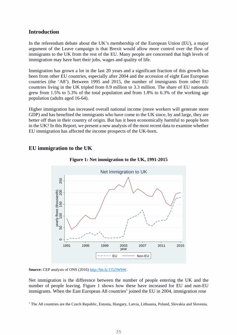
Introduction In the referendum debate about the UK’s membership of the European Union (EU), a major argument of the Leave campaign is that Brexit would allow more control over the flow of immigrants to the UK from the rest of the EU. Many people are concerned that high levels of immigration may have hurt their jobs, wages and quality of life. Immigration has grown a lot in the last 20 years and a significant fraction of this growth has been from other EU countries, especially after 2004 and the accession of eight East European countries (the ‘A8’). Between 1995 and 2015, the number of immigrants from other EU countries living in the UK tripled from 0.9 million to 3.3 million. The share of EU nationals grew from 1.5% to 5.3% of the total population and from 1.8% to 6.3% of the working age population (adults aged 16-64). Higher immigration has increased overall national income (more workers will generate more GDP) and has benefited the immigrants who have come to the UK since, by and large, they are better off than in their country of origin. But has it been economically harmful to people born in the UK? In this Report, we present a new analysis of the most recent data to examine whether EU immigration has affected the income prospects of the UK-born. EU immigration to the UK

Figure 1: Net immigration to the UK, 1991-2015

Source: CEP analysis of ONS (2016) http://bit.ly/1Tz5WbW. Net immigration is the difference between the number of people entering the UK and the number of people leaving. Figure 1 shows how these have increased for EU and non-EU immigrants. When the East European A8 countries1 joined the EU in 2004, immigration rose

1 The A8 countries are the Czech Republic, Estonia, Hungary, Latvia, Lithuania, Poland, Slovakia and Slovenia.

050

100

150

200

250

year

ly fl

ows

(thou

sand

s)

1991 1995 1999 2003 2007 2011 2015year

EU Non-EU

Net Immigration to UK

35

http://bit.ly/1Tz5WbW

significantly, but it then fell back during the recession after 2007. In the last few years, net inflows have again risen significantly as the economy has recovered. In the year to September 2015, net EU immigration was 172,000, comprising 257,000 EU nationals arriving and 85,000 leaving. This is only just below the figure of 191,000 net immigration for non-EU nationals. The best source of data to explore the impact of immigration is the Labour Force Survey (LFS). This is because it makes it possible to measure the economic circumstances of people born in the UK and compare them with immigrants from the EU and other countries. The Annex gives more details and compares the LFS with other data sources, such as National Insurance numbers. The conclusions of this report are robust to using other data sources such as NI numbers for migration and the Annual Survey of Hours and Earnings for wages. In 2015, there were around 3.3 million EU immigrants living in the UK up from 0.9 million in 1995 - a rise to 5.3% of the population from 1.5%. Around 2.5 million of these migrants are aged 16-64 and two million are in work.2 EU countries now account for 35% of all immigrants living in the UK. While 29% of EU nationals are Polish and 12% are Irish, the nationalities of other EU immigrants are quite evenly spread across the other 25 countries in the EU (Figure 2). As with other immigrants, there is a greater concentration of EU nationals in London than in the rest of the country (Figure 3). A third of EU nationals live in London compared with only 11% of UK nationals.

Figure 2: EU immigrants by nationality, 2015

Source: CEP analysis of Labour Force Survey.

2 The focus is on EU nationals (self-defined) rather than country of birth, since any decision to restrict entry would presumably be based on nationality and not country of birth.

36

Figure 3: Proportion of UK and EU nationals in each region, 2015 Source: CEP analysis of Labour Force Survey. Notes: London is marked in black. This is where immigrants are disproportionately concentrated. EU immigrants are on average more educated than the UK-born (Table 1) – almost twice as many of them have some form of higher education (43% compared with 23% UK-born). Only 15% of EU immigrants left school at 16 compared with 44% of the UK-born.

Table 1: Education and immigrant status (working age population) 2015

Age finished education

UK-Born EU immigrants A8 immigrants All immigrants

High ( 21 or older) 23% 43% 36% 45% Medium (17-20) 33% 42% 55% 36% Low (16 or under) 44% 15% 9% 19% All 100% 100% 100% 100%

Source: CEP analysis of Labour Force Survey. Notes: The A8 countries are the Czech Republic, Estonia, Hungary, Latvia, Lithuania, Poland, Slovakia and Slovenia, all of which joined the EU in 2004. Working age population is all individuals between the ages of 16 and 64. Table 2 shows that EU immigrants are not only more educated, but they are also more likely to be in work (78.2%) than UK-born individuals (72.5%) and less likely to be unemployed or economically inactive. This is particularly true of A8 immigrants: almost 82% of them are in work.

0 5 10 15 20 0 5 10 15 20

Northern IrelandRest of Scotland

StrathclydeWales

Rest of North WestMerseyside

Greater ManchesterRest of West Midlands

West Midlands (met county)South West

Rest of South East

Outer LondonInner London

East AngliaEast Midlands

Rest of Yorks & HumbersideWest Yorkshire

South YorkshireRest of Northern region

Tyne & Wear

Northern IrelandRest of Scotland

StrathclydeWales

Rest of North WestMerseyside

Greater ManchesterRest of West Midlands

West Midlands (met county)South West

Rest of South East

Outer LondonInner London

East AngliaEast Midlands

Rest of Yorks & HumbersideWest Yorkshire

South YorkshireRest of Northern region

Tyne & Wear

UK-Born EU Immigrants

Percent living in each region

37

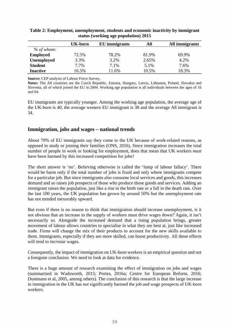
Table 2: Employment, unemployment, students and economic inactivity by immigrant status (working age population) 2015

UK-born EU immigrants A8 All immigrants % of whom:

Employed 72.5% 78.2% 81.9% 69.9% Unemployed 3.3% 3.2% 2.65% 4.2% Student 7.7% 7.1% 5.1% 7.6% Inactive 16.5% 11.6% 10.5% 18.3%

Source: CEP analysis of Labour Force Survey. Notes: The A8 countries are the Czech Republic, Estonia, Hungary, Latvia, Lithuania, Poland, Slovakia and Slovenia, all of which joined the EU in 2004. Working age population is all individuals between the ages of 16 and 64. EU immigrants are typically younger. Among the working age population, the average age of the UK-born is 40, the average western EU immigrant is 38 and the average A8 immigrant is 34. Immigration, jobs and wages – national trends About 70% of EU immigrants say they come to the UK because of work-related reasons, as opposed to study or joining their families (ONS, 2016). Since immigration increases the total number of people in work or looking for employment, does that mean that UK workers must have been harmed by this increased competition for jobs? The short answer is ‘no’. Believing otherwise is called the ‘lump of labour fallacy’. There would be harm only if the total number of jobs is fixed and only where immigrants compete for a particular job. But since immigrants also consume local services and goods, this increases demand and so raises job prospects of those who produce those goods and services. Adding an immigrant raises the population, just like a rise in the birth rate or a fall in the death rate. Over the last 100 years, the UK population has grown by around 50% but the unemployment rate has not trended inexorably upward. But even if there is no reason to think that immigration should increase unemployment, is it not obvious that an increase in the supply of workers must drive wages down? Again, it isn’t necessarily so. Alongside the increased demand that a rising population brings, greater movement of labour allows countries to specialise in what they are best at, just like increased trade. Firms will change the mix of their products to account for the new skills available to them. Immigrants, especially if they are more skilled, can boost productivity. All these effects will tend to increase wages. Consequently, the impact of immigration on UK-born workers is an empirical question and not a foregone conclusion. We need to look at data for evidence. There is a huge amount of research examining the effect of immigration on jobs and wages (summarised in Wadsworth, 2015; Portes, 2016a; Centre for European Reform, 2016; Dustmann et al, 2005, among others). The conclusion of this research is that the large increase in immigration in the UK has not significantly harmed the job and wage prospects of UK-born workers.

38

Most of this work, however, was conducted prior to the global financial crisis and the Eurozone crisis. So it is reasonable to ask whether these findings have changed after the most severe economic downturn for 80 years. Figures 4 to 6 plot the unemployment, employment and wage trends for individuals born in the UK alongside the trend in immigration from the EU. In Figure 4, at a time when EU immigration has been rising sharply (after 2004), UK unemployment for those born in the UK rose – but then fell back to a very low level, while EU immigration kept on rising. Indeed, despite the global crash, the rise in unemployment for UK-born workers was much less than in previous downturns when EU immigration was much lower. Figure 4: Unemployment of UK-born and EU immigration, 1975-2015

Source: CEP analysis of Labour Force Survey. Notes: % EU is the proportion of EU nationals in the working age population (16-64 for men, 16-59 for women). A similar pattern can be seen using the fraction of the working population in jobs (the employment rate) for UK-born workers (Figure 5).3 The employment rate of UK-born workers goes up and down with the economic cycle, but has risen recently in the period when EU immigration is also rising. It is almost back to levels seen at the peak of previous recoveries. Median real wages for those born in the UK were growing from the late 1990s until the global financial crisis. Since then, wages have fallen by about 10%. Such falls in real wages are unprecedented in the post-war period. The story of the latest recession was not that many more people lost their jobs, but that most people’s wages fell. Figure 6 confirms that this fall happened while EU immigration was rising – but equally the big gains in real wages for UK workers were experienced at a time when EU immigration was also rising. So the cause of the fall of wages is the impact of the Great Recession – not immigration.

3 The employment count in Figure 5 excludes any students in work – but the trends are very similar if any students in work are added back in to employment.

12

34

56

% E

U n

atio

nals

in w

orki

ng a

ge p

opul

atio

n

46

810

12U

K-Bo

rn u

nem

ploy

men

t rat

e (%

)

1975 1980 1985 1990 1995 2000 2005 2010 2015

Unemployment EU share in pop.

Onset of global financial crisis

39

Figure 5: Employment rate of UK-born and EU immigration, 1975-2015

Source: CEP analysis of Labour Force Survey. Notes: % EU is the proportion of EU nationals in the working age population (16-64 for men, 16-59 for women).

Figure 6: Median real hourly wages for the UK-born, 1995-2015

Source: CEP analysis of Labour Force Survey. Notes: Median wage is deflated by the CPI.

12

34

56

% E

U n

atio

nals

in w

orki

ng a

ge p

opul

atio

n

6870

7274

UK

-Bor

n em

ploy

men

t rat

e (%

)

1975 1980 1985 1990 1995 2000 2005 2010 2015

Employment EU share in pop.

23

45

6%

of E

U n

atio

nals

in w

orki

ng a

ge p

op

89

1011

12re

al h

ourly

wag

es (£

2015

)

1995 1999 2003 2007 2011 2015year

Real Wages EU share in pop.

Real Hourly Wages UK-Born Workers

40

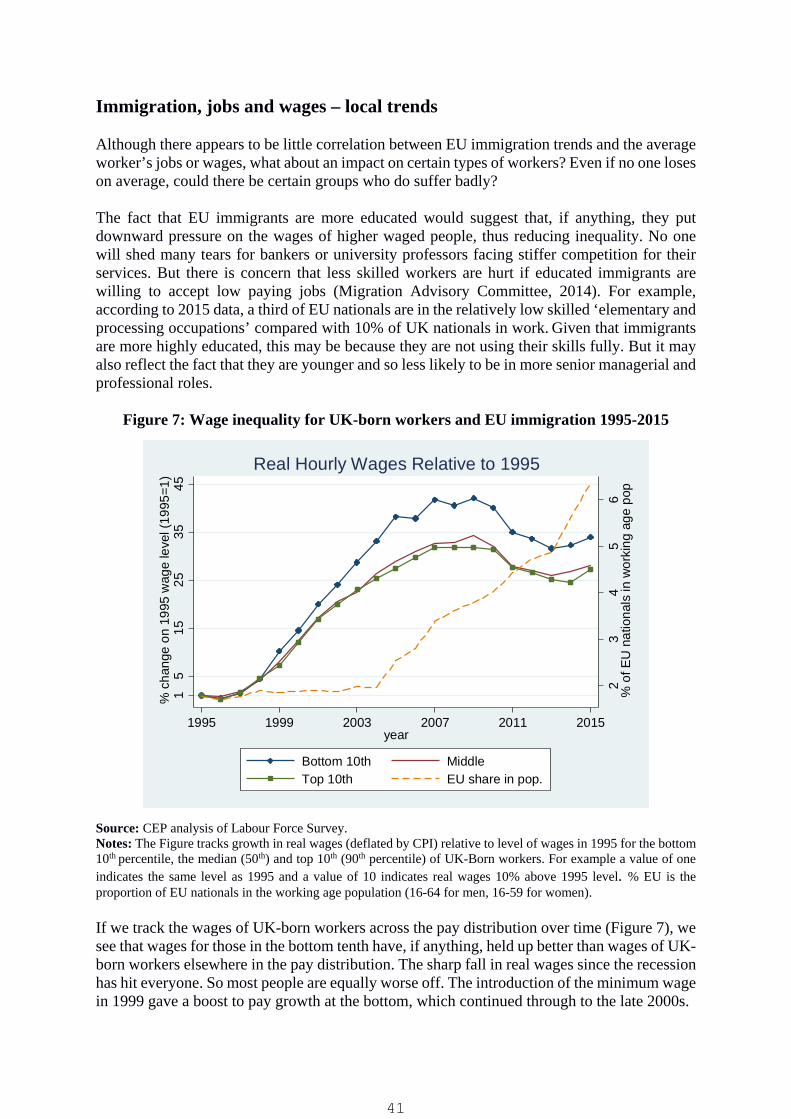
Immigration, jobs and wages – local trends Although there appears to be little correlation between EU immigration trends and the average worker’s jobs or wages, what about an impact on certain types of workers? Even if no one loses on average, could there be certain groups who do suffer badly? The fact that EU immigrants are more educated would suggest that, if anything, they put downward pressure on the wages of higher waged people, thus reducing inequality. No one will shed many tears for bankers or university professors facing stiffer competition for their services. But there is concern that less skilled workers are hurt if educated immigrants are willing to accept low paying jobs (Migration Advisory Committee, 2014). For example, according to 2015 data, a third of EU nationals are in the relatively low skilled ‘elementary and processing occupations’ compared with 10% of UK nationals in work. Given that immigrants are more highly educated, this may be because they are not using their skills fully. But it may also reflect the fact that they are younger and so less likely to be in more senior managerial and professional roles.

Figure 7: Wage inequality for UK-born workers and EU immigration 1995-2015

Source: CEP analysis of Labour Force Survey. Notes: The Figure tracks growth in real wages (deflated by CPI) relative to level of wages in 1995 for the bottom 10th percentile, the median (50th) and top 10th (90th percentile) of UK-Born workers. For example a value of one indicates the same level as 1995 and a value of 10 indicates real wages 10% above 1995 level. % EU is the proportion of EU nationals in the working age population (16-64 for men, 16-59 for women). If we track the wages of UK-born workers across the pay distribution over time (Figure 7), we see that wages for those in the bottom tenth have, if anything, held up better than wages of UK-born workers elsewhere in the pay distribution. The sharp fall in real wages since the recession has hit everyone. So most people are equally worse off. The introduction of the minimum wage in 1999 gave a boost to pay growth at the bottom, which continued through to the late 2000s.

23

45

6%

of E

U n

atio

nals

in w

orki

ng a

ge p

op

15

1525

3545

% c

hang

e on

199

5 w

age

leve

l (19

95=1

)

1995 1999 2003 2007 2011 2015year

Bottom 10th MiddleTop 10th EU share in pop.

Real Hourly Wages Relative to 1995

41

Again, the rise in EU immigration happened in periods of relative wage growth at the bottom wage levels and in periods of relative wage stability at the bottom. So it is hard to see evidence of relative wage falls for low paid UK workers when EU immigration is rising. On the face of it, it would seem that the recession coincides with much of the recent bad experiences of UK-born workers with regard to jobs and pay rather than rising immigration. Looking at economy-wide changes might disguise effects in local areas where immigration has gone up by a lot. The most straightforward way to investigate this issue is to examine whether areas of the UK that had larger influxes of EU immigrants also had worse job and wage outcomes for the UK-born relative to other areas. Looking at the change over time controls for lots of other features of the local labour market that could also explain unemployment and wages in those areas. Figure 8 considers changes in the unemployment rates of the UK-born across local authorities in relation to changes in EU immigration between 2008 and 2015 (one dot for each of the 201 local authorities). The solid red line summarises the relationship between immigration and UK-born unemployment rates. If immigration increased unemployment, we would expect a strong upward sloping line: more EU immigrants would mean more unemployment for local workers. In fact, the line indicates that a 10 percentage point increase in the share of EU immigrants in a local area is associated with a 0.4 percentage point reduction in the unemployment rate in that area. But it is very clear from the graph that there is absolutely no statistically significant relationship (negative or positive) of EU immigration on unemployment rates of those born in the UK.

Figure 8: Unemployment rates of UK-born & EU immigration

Source: CEP analysis of Labour Force Survey. Notes: Each dot represents a UK local authority. The solid line is the predicted ‘best fit’ from a regression of changes in unemployment on the change in share of EU immigrants in each UK local authority. These are weighted by the sample population in each area. Slope of this line is -0.04 with standard error of 0.05, statistically insignificantly different from zero.

B

A

-8-6

-4-2

02

46

8%

poi

nt c

hang

e in

loca

l are

a U

nem

ploy

men

t Rat

e: 2

008-

2015

-2 0 2 4 6 8 10 12 14% point change in local area EU Immigrant Share 2008-2015

local area values Fitted value

Change in UK-Born Unemployment Rate 2008-2015

42

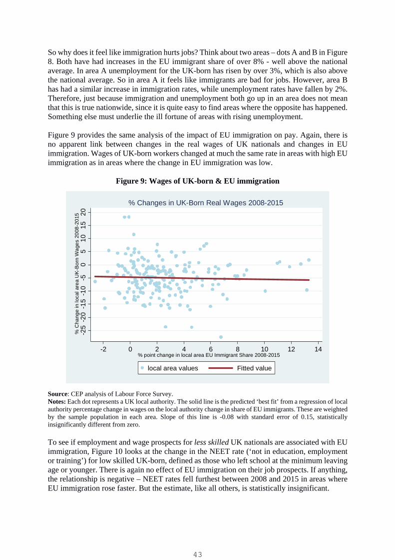
So why does it feel like immigration hurts jobs? Think about two areas – dots A and B in Figure 8. Both have had increases in the EU immigrant share of over 8% - well above the national average. In area A unemployment for the UK-born has risen by over 3%, which is also above the national average. So in area A it feels like immigrants are bad for jobs. However, area B has had a similar increase in immigration rates, while unemployment rates have fallen by 2%. Therefore, just because immigration and unemployment both go up in an area does not mean that this is true nationwide, since it is quite easy to find areas where the opposite has happened. Something else must underlie the ill fortune of areas with rising unemployment. Figure 9 provides the same analysis of the impact of EU immigration on pay. Again, there is no apparent link between changes in the real wages of UK nationals and changes in EU immigration. Wages of UK-born workers changed at much the same rate in areas with high EU immigration as in areas where the change in EU immigration was low.

Figure 9: Wages of UK-born & EU immigration

Source: CEP analysis of Labour Force Survey. Notes: Each dot represents a UK local authority. The solid line is the predicted ‘best fit’ from a regression of local authority percentage change in wages on the local authority change in share of EU immigrants. These are weighted by the sample population in each area. Slope of this line is -0.08 with standard error of 0.15, statistically insignificantly different from zero. To see if employment and wage prospects for less skilled UK nationals are associated with EU immigration, Figure 10 looks at the change in the NEET rate (‘not in education, employment or training’) for low skilled UK-born, defined as those who left school at the minimum leaving age or younger. There is again no effect of EU immigration on their job prospects. If anything, the relationship is negative – NEET rates fell furthest between 2008 and 2015 in areas where EU immigration rose faster. But the estimate, like all others, is statistically insignificant.

-25

-20

-15

-10

-50

510

1520

% C

hang

e in

loca

l are

a U

K-B

orn

Wag

es 2

008-

2015



% Changes in UK-Born Real Wages 2008-2015

43

Likewise, Figure 11 shows no obvious link between the pay of less skilled UK-born individuals and changes in the local area population of EU nationals over this period. The Technical Appendix presents a large number of variations of these graphs. For example, we repeat the analysis for other periods such as starting in 2004 when the A8 joined the EU or 2011 when the Eurozone crisis really worsened. We drop London to make sure that the capital is not biasing the relationships. Across all experiments, the results are essentially unchanged: EU immigration does not seem to harm UK workers. Figure 10: NEET (‘not in education, employment or training’) rates for less skilled UK-

born & EU immigration, 2008-2015

Source: CEP analysis of Labour Force Survey. Notes: Each dot represents a UK local authority. The solid line is the predicted ‘best fit’ from a regression of local authority change in NEET rates for the less skilled on the local authority change in share of EU immigrants. These are weighted by the sample population in each area. Slope of this line is -0.10 with standard error of 0.14, statistically insignificantly different from zero. NEET stands for those ‘not in education, employment or training.’ Less skilled is defined by those who left school at 16 or earlier.

-20

-15

-10

-50

510

15%

Cha

nge

in lo

cal a

rea

UK

-bor

n N

EE

T R

ate:

200

8-20

15



Change in UK-Born NEET Rate for Less Skilled 2008-2015

44

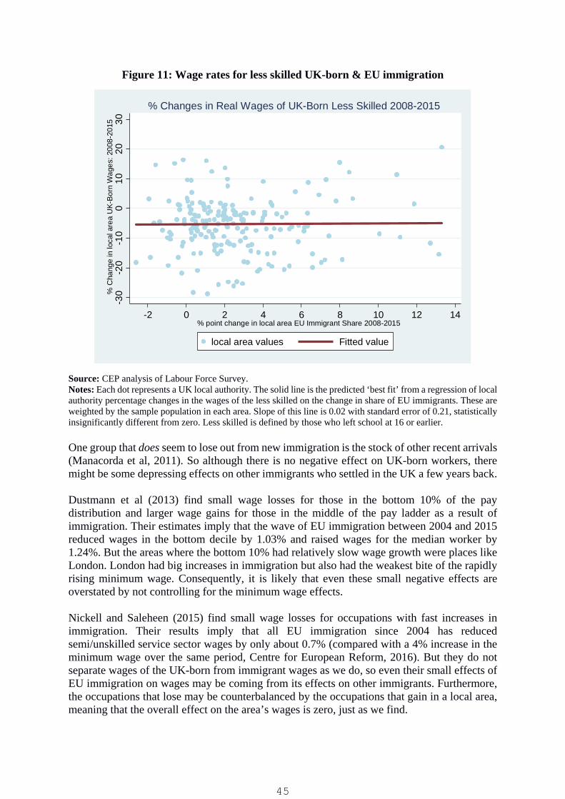
Figure 11: Wage rates for less skilled UK-born & EU immigration

Source: CEP analysis of Labour Force Survey. Notes: Each dot represents a UK local authority. The solid line is the predicted ‘best fit’ from a regression of local authority percentage changes in the wages of the less skilled on the change in share of EU immigrants. These are weighted by the sample population in each area. Slope of this line is 0.02 with standard error of 0.21, statistically insignificantly different from zero. Less skilled is defined by those who left school at 16 or earlier. One group that does seem to lose out from new immigration is the stock of other recent arrivals (Manacorda et al, 2011). So although there is no negative effect on UK-born workers, there might be some depressing effects on other immigrants who settled in the UK a few years back. Dustmann et al (2013) find small wage losses for those in the bottom 10% of the pay distribution and larger wage gains for those in the middle of the pay ladder as a result of immigration. Their estimates imply that the wave of EU immigration between 2004 and 2015 reduced wages in the bottom decile by 1.03% and raised wages for the median worker by 1.24%. But the areas where the bottom 10% had relatively slow wage growth were places like London. London had big increases in immigration but also had the weakest bite of the rapidly rising minimum wage. Consequently, it is likely that even these small negative effects are overstated by not controlling for the minimum wage effects. Nickell and Saleheen (2015) find small wage losses for occupations with fast increases in immigration. Their results imply that all EU immigration since 2004 has reduced semi/unskilled service sector wages by only about 0.7% (compared with a 4% increase in the minimum wage over the same period, Centre for European Reform, 2016). But they do not separate wages of the UK-born from immigrant wages as we do, so even their small effects of EU immigration on wages may be coming from its effects on other immigrants. Furthermore, the occupations that lose may be counterbalanced by the occupations that gain in a local area, meaning that the overall effect on the area’s wages is zero, just as we find.

-30

-20

-10

010

2030

% C

hang

e in

loca

l are

a U

K-B

orn

Wag

es: 2

008-

2015



% Changes in Real Wages of UK-Born Less Skilled 2008-2015

45

The impact of EU immigration on public finances and public services What is the fiscal impact of immigration on public finances and public services? Public expenditure will be lower on one point since UK taxpayers have not had to finance the childhood schooling and healthcare costs of an immigrant adult as they would do for a UK-born adult. Second, we have documented above that EU immigrants are younger, more likely to work and less likely to be on benefits. While immigrants, like UK nationals, would not be eligible for contributory-related benefits until they have worked full-time for two years, they could be eligible for means-tested benefits should they apply. HMRC estimates that around 6% of tax credit claims are from households that include an EU national in line with the share of EU nationals in the UK (House of Commons, 2014). After trying to account for the many possible ways in which individuals pay taxes or draw welfare, Dustmann and Frattini (2014) find that EU immigrants made a positive fiscal contribution: they paid more in taxes than they received in welfare payments. For example, A8 immigrants paid in about £15 billion more than they took out in public spending in the decade up to 2011. While this effect may seem small, the longer-run impact could be substantial. The central estimate of the Office for Budget Responsibility (2013) is that the UK’s national debt will be 40 percentage points higher in 2062 if net immigration is reduced to zero from 140,000 per year. By contrast, UK nationals, as a whole, received more in benefits than they paid in taxes. Given that EU immigrants are making net contributions, there is no reason to think that they should crowd out any public services. In fact, they are bringing extra resources that could be used to increase spending on local health and education for the UK-born. In other words, reducing EU immigration would generate the need for greater austerity. This would magnify the need for cutbacks caused by the slower growth of the economy due to reduced trade and investment identified by Dhingra et al (2016a, 2016b). Although the fact that the government has been cutting back on public services cannot therefore be blamed on immigrants, it is still interesting to see whether immigration has led to worse local services. If immigrants cause social disruption, we would expect this to be reflected in crime rates. Bell et al (2013) find no effect of the big 2004 increase in immigration from East European countries on crime. Geay et al (2013) find no effect of immigration on aspects of educational attainment and actually some positive effect from Polish children on UK-born pupils. The disadvantage in having English as a second language seems to be outweighed by a stronger immigrant push to work hard at school. For the NHS, Wadsworth (2013) finds no greater usage of doctors and hospitals by immigrants relative to the UK-born; and Giuntella et al (2015) find little effect on NHS waiting times. These studies do not distinguish between EU and non-EU immigrants, but since EU immigrants are younger than non-EU immigrants, they are less likely to use health services, so the results are likely to be stronger.

46

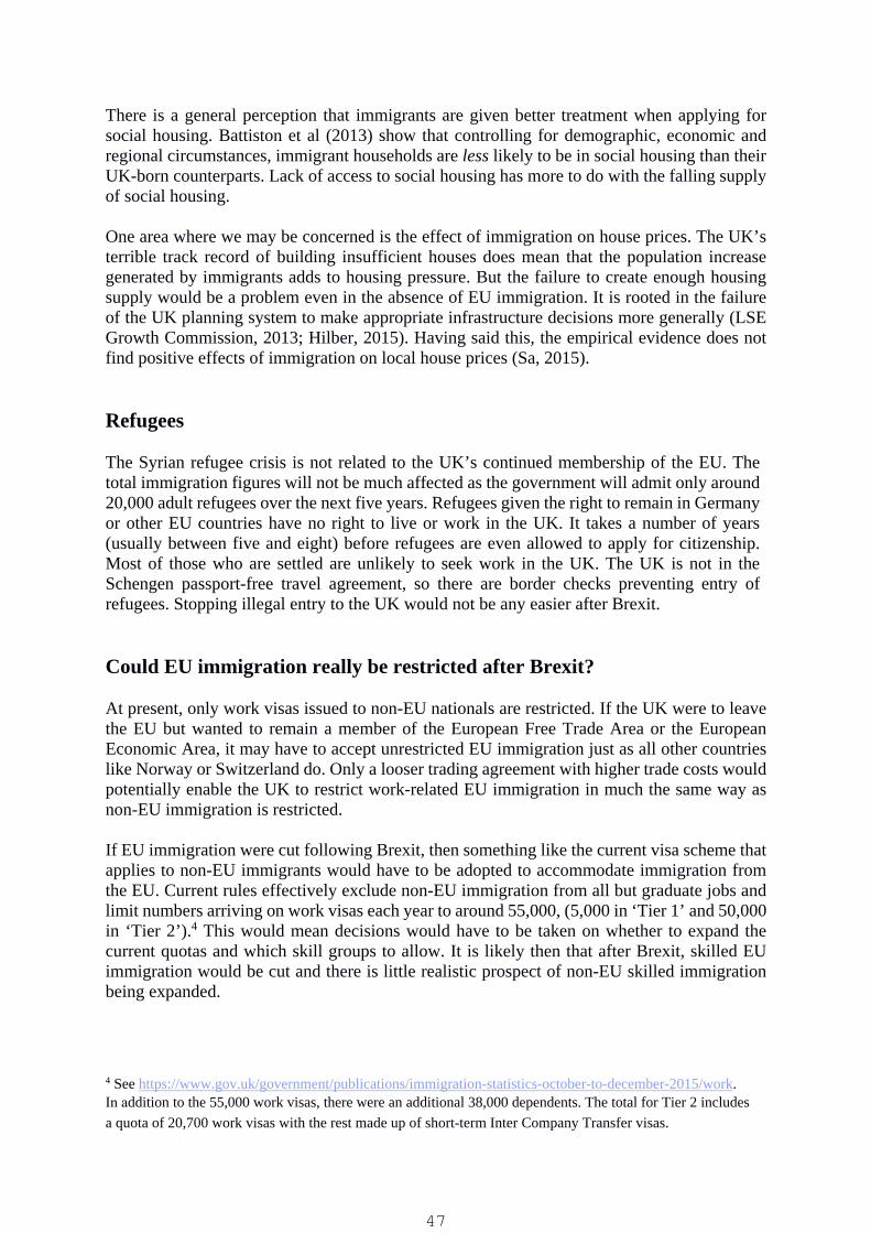
There is a general perception that immigrants are given better treatment when applying for social housing. Battiston et al (2013) show that controlling for demographic, economic and regional circumstances, immigrant households are less likely to be in social housing than their UK-born counterparts. Lack of access to social housing has more to do with the falling supply of social housing.

One area where we may be concerned is the effect of immigration on house prices. The UK’s terrible track record of building insufficient houses does mean that the population increase generated by immigrants adds to housing pressure. But the failure to create enough housing supply would be a problem even in the absence of EU immigration. It is rooted in the failure of the UK planning system to make appropriate infrastructure decisions more generally (LSE Growth Commission, 2013; Hilber, 2015). Having said this, the empirical evidence does not find positive effects of immigration on local house prices (Sa, 2015).

Refugees

The Syrian refugee crisis is not related to the UK’s continued membership of the EU. The total immigration figures will not be much affected as the government will admit only around 20,000 adult refugees over the next five years. Refugees given the right to remain in Germany or other EU countries have no right to live or work in the UK. It takes a number of years (usually between five and eight) before refugees are even allowed to apply for citizenship. Most of those who are settled are unlikely to seek work in the UK. The UK is not in the Schengen passport-free travel agreement, so there are border checks preventing entry of refugees. Stopping illegal entry to the UK would not be any easier after Brexit.

Could EU immigration really be restricted after Brexit?

At present, only work visas issued to non-EU nationals are restricted. If the UK were to leave the EU but wanted to remain a member of the European Free Trade Area or the European Economic Area, it may have to accept unrestricted EU immigration just as all other countries like Norway or Switzerland do. Only a looser trading agreement with higher trade costs would potentially enable the UK to restrict work-related EU immigration in much the same way as non-EU immigration is restricted.

If EU immigration were cut following Brexit, then something like the current visa scheme that applies to non-EU immigrants would have to be adopted to accommodate immigration from the EU. Current rules effectively exclude non-EU immigration from all but graduate jobs and limit numbers arriving on work visas each year to around 55,000, (5,000 in ‘Tier 1’ and 50,000 in ‘Tier 2’).4 This would mean decisions would have to be taken on whether to expand the current quotas and which skill groups to allow. It is likely then that after Brexit, skilled EU immigration would be cut and there is little realistic prospect of non-EU skilled immigration being expanded.

4 See https://www.gov.uk/government/publications/immigration-statistics-october-to-december-2015/work. In addition to the 55,000 work visas, there were an additional 38,000 dependents. The total for Tier 2 includes a quota of 20,700 work visas with the rest made up of short-term Inter Company Transfer visas.

47

http://bit.ly/28LKmVM

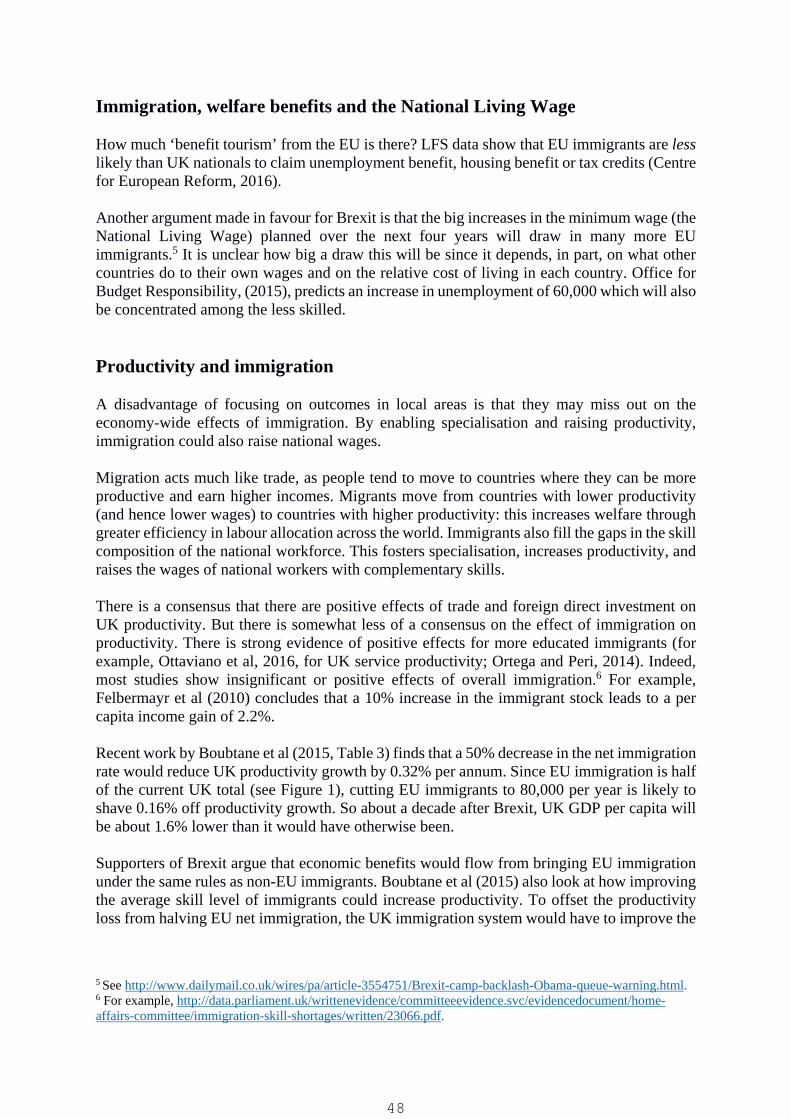
Immigration, welfare benefits and the National Living Wage How much ‘benefit tourism’ from the EU is there? LFS data show that EU immigrants are less likely than UK nationals to claim unemployment benefit, housing benefit or tax credits (Centre for European Reform, 2016). Another argument made in favour for Brexit is that the big increases in the minimum wage (the National Living Wage) planned over the next four years will draw in many more EU immigrants.5 It is unclear how big a draw this will be since it depends, in part, on what other countries do to their own wages and on the relative cost of living in each country. Office for Budget Responsibility, (2015), predicts an increase in unemployment of 60,000 which will also be concentrated among the less skilled. Productivity and immigration A disadvantage of focusing on outcomes in local areas is that they may miss out on the economy-wide effects of immigration. By enabling specialisation and raising productivity, immigration could also raise national wages. Migration acts much like trade, as people tend to move to countries where they can be more productive and earn higher incomes. Migrants move from countries with lower productivity (and hence lower wages) to countries with higher productivity: this increases welfare through greater efficiency in labour allocation across the world. Immigrants also fill the gaps in the skill composition of the national workforce. This fosters specialisation, increases productivity, and raises the wages of national workers with complementary skills. There is a consensus that there are positive effects of trade and foreign direct investment on UK productivity. But there is somewhat less of a consensus on the effect of immigration on productivity. There is strong evidence of positive effects for more educated immigrants (for example, Ottaviano et al, 2016, for UK service productivity; Ortega and Peri, 2014). Indeed, most studies show insignificant or positive effects of overall immigration.6 For example, Felbermayr et al (2010) concludes that a 10% increase in the immigrant stock leads to a per capita income gain of 2.2%. Recent work by Boubtane et al (2015, Table 3) finds that a 50% decrease in the net immigration rate would reduce UK productivity growth by 0.32% per annum. Since EU immigration is half of the current UK total (see Figure 1), cutting EU immigrants to 80,000 per year is likely to shave 0.16% off productivity growth. So about a decade after Brexit, UK GDP per capita will be about 1.6% lower than it would have otherwise been. Supporters of Brexit argue that economic benefits would flow from bringing EU immigration under the same rules as non-EU immigrants. Boubtane et al (2015) also look at how improving the average skill level of immigrants could increase productivity. To offset the productivity loss from halving EU net immigration, the UK immigration system would have to improve the

5 See http://www.dailymail.co.uk/wires/pa/article-3554751/Brexit-camp-backlash-Obama-queue-warning.html. 6 For example, http://data.parliament.uk/writtenevidence/committeeevidence.svc/evidencedocument/home-affairs-committee/immigration-skill-shortages/written/23066.pdf.

48

http://dailym.ai/28JsKY8

http://bit.ly/28Lzy9y

relative education levels of EU immigrants by about a quarter. Since EU immigrants are already significantly better educated than the UK-born, this may be hard to engineer. Conclusion We cannot be precise about the size of the losses from restricting immigration following a Brexit. But we can confidently say that the empirical evidence shows that EU immigration has not had significantly negative effects on average employment, wages, inequality or public services at the local level for the UK-born. Nor, it should be said, are there large positive effects. Any adverse experiences of UK-born workers with regard to jobs and wages are more closely associated with the biggest economic crash for more than 80 years. At the national level, falls in EU immigration are likely to lead to lower living standards for the UK-born. This is partly because immigrants help to reduce the deficit: they are more likely to work and pay tax and less likely to use public services as they are younger and better educated than the UK-born. It is also partly due to the positive effects of EU immigrants on productivity. Our earlier reports reflect a wide consensus that trade and foreign investment will also fall after Brexit, both of which would reduce UK incomes. Lower immigration is a third channel that will push UK living standards even lower. May 2016 For further information, contact: Jonathan Wadsworth ([email protected]), Swati Dhingra ([email protected]), Gianmarco Ottaviano ([email protected]), John Van Reenen ([email protected]) or Romesh Vaitilingam on 07768-661095 ([email protected]). Jonathan Wadsworth was a member of the Home Office’s Migration Advisory Committee 2007 to 2015.

49

Further reading Battiston, D., R. Dickens, A. Manning and J. Wadsworth (2013) ‘Immigration and the Access to Social Housing in the UK’, CEP Discussion Paper No. 1264 (http://cep.lse.ac.uk/pubs/download/dp1264.pdf). Bell B., F. Fasani and S. Machin (2013) ‘Crime and Immigration: Evidence from Large Immigrant Waves’, Review of Economics and Statistics 95(4): 1278-90. Boubtane, E., J-C. Dumont and C. Rault (2015) ‘Immigration and Economic Growth in the OECD Countries 1986-2006’ CESIFO Working Paper 5392 (http://papers.ssrn.com/sol3/Delivery.cfm/SSRN_ID2622005_code459177.pdf?abstractid=2622005&mirid=3). Centre for European Reform (2016) The Economic Consequences of Leaving the EU (https://www.cer.org.uk/publications/archive/report/2016/economic-consequences-leaving-eu-final-report-cer-commission-brexit). Dhingra, S., G. Ottaviano, T. Sampson and J. Van Reenen (2016a) ‘The Consequences of Brexit for UK Trade and Living Standards’ CEP Brexit Analysis No. 2 (http://cep.lse.ac.uk/pubs/download/brexit02.pdf). Dhingra, S., G. Ottaviano, T. Sampson and J. Van Reenen (2016b) ‘The Impact of Brexit on Foreign Investment in the UK’, CEP Brexit Analysis No. 3 (http://cep.lse.ac.uk/pubs/download/brexit03.pdf). Dustmann, C., F. Fabbri and I. Preston (2005) ‘The Impact of Immigration on the UK Labour Market’, Economic Journal 115: F324-41. Dustmann, C., T. Frattini and I. Preston (2013) ‘The Effect of Immigration along the Distribution of Wages’, Review of Economic Studies 80: 145-73. Dustmann, C. and T. Frattini (2014) ‘The Fiscal Effects of Immigration to the UK.’ Economic Journal 124: F593-643. Geay, C., S. McNally and S. Telhaj (2013) ‘Non-Native Speakers in the Classroom: What are the Effects on Pupil Performance?’ Economic Journal 123: F281-307. Felbermayr, G., S. Hiller and D. Sala (2010) ‘Does Immigration Boost per Capita Income?’ Economic Letters 107(2): 177-79.

Giuntella, O., C. Nicodemo and C. Vargas Silva (2015) ‘The Effects of Immigration on NHS Waiting Times’, University of Oxford Working Paper. Hilber, C (2015) ‘UK Housing and Planning Policies’ CEP Election Analysis No. 3 (http://cep.lse.ac.uk/pubs/download/EA033.pdf). House of Commons (2014) ‘Statistics on migrants and benefits’, House of Commons Note Standard (http://researchbriefings.parliament.uk/ResearchBriefing/Summary/SN06955).

50



http://papers.ssrn.com/sol3/papers.cfm?abstract_id=2622005

http://bit.ly/28LL5X7



http://researchbriefings.parliament.uk/ResearchBriefing/Summary/SN06955

LSE Growth Commission (2013) Investing for Prosperity, (http://www.lse.ac.uk/researchAndExpertise/units/growthCommission/documents/pdf/LSEGC-Report.pdf). Manacorda, M., A. Manning and J. Wadsworth (2011) ‘The Impact of Immigration on the Structure of Male Wages: Theory and Evidence from Britain’, Journal of the European Economic Association 10: 120-51. Migration Advisory Committee (2014), ‘Migrants in Low Skilled Work’ (https://www.gov.uk/government/uploads/system/uploads/attachment_data/file/333083/MAC-Migrants_in_low-skilled_work__Full_report_2014.pdf). Nickell, S. and J. Saleheen (2015) ‘The Impact of Immigration on Occupational Wages: Evidence from Britain’, Bank of England Staff Working Paper No. 574. Office for Budget Responsibility (2013) ‘Fiscal Sustainability Report’, July. Office for Budget Responsibility (2015) ‘Economic and Fiscal Outlook’, July. ONS (2016) Migration Statistics Quarterly Review (https://www.ons.gov.uk/peoplepopulationandcommunity/populationandmigration/internationalmigration/bulletins/migrationstatisticsquarterlyreport/february2016). Ortega F. and G. Peri (2014) ‘Migration, Trade and Income’, Journal of International Economics 92: 231-51. Ottaviano, G., G. Peri and G. Wright (2016) ‘Immigration, Trade and productivity in services’, CEP Discussion Paper 1353 (http://cep.lse.ac.uk/pubs/download/dp1353.pdf). Portes, J. (2016a) ‘Immigration, Free Movement and the UK Referendum’, NIESR Review 236. Portes, J. (2016b) ‘EU Immigration and the UK Labour Market’, NIESR mimeo. Sa, F., (2015) ‘Immigration and House Prices in the UK’, Economic Journal 125: 1393-1424. Wadsworth, J. (2013) ‘Mustn’t Grumble: Immigration, Health and Health Service Use in the UK and Germany’, Fiscal Studies 34(1): 55-82. Wadsworth, J. (2015) ‘Immigration and the UK Labour Market’, CEP Election Analysis No. 1 (http://cep.lse.ac.uk/pubs/download/EA019.pdf).

51

http://bit.ly/1lOaQFN

https://www.gov.uk/government/uploads/system/uploads/attachment_data/file/333083/MAC-Migrants_in_low-skilled_work__Full_report_2014.pdf

http://bit.ly/1XSMvif



Annex: Data Sources and Definitions Labour Force Survey (LFS) Most of this report is based on CEP analysis of the latest individual-level data from Labour Force Survey (LFS). The LFS is the best data source to use covering a representative sample of individuals living in the UK. For example, in 2015, it includes about 90,000 people. The analysis in Figures 8-11 uses the Annual Population Survey (APS) which is based on pooling the LFS quarterly panel over about a year. It has about 350,000 observations a year for the working age population. In the regression lines we weight by the sample population to correct the standard errors for small areas. With the LFS, it is possible to separate out who is a UK-born individual from those who are EU nationals. This enables us to examine not just the reported trends in the labour market but also to break this down into the UK-born and immigrants. National Insurance numbers There is some discrepancy between the number of National Insurance (NI) numbers issued to EU nationals and survey estimates of the EU immigrant population and inflows based on the LFS and International Passenger Survey (IPS) respectively. Anyone should claim a NI number if they are in work, looking to work or wish to be eligible for tax credits or benefits. The NI count is based on these inflows. It has the advantage over the LFS that it is administrative data on the population of NI numbers and therefore not a sample. But compared with the LFS, it will underestimate the flows for EU immigrants who are working but do not have NI numbers or those who are not seeking to work. A big disadvantage of NI numbers is that individuals keep their NI number when they leave the country. Consequently, we do not know the immigrant outflows using NI numbers. Thus, it is not possible to make a reliable calculation of the net immigration numbers using NI counts. According to the IPS, about 90,000 EU nationals leave the UK each year, taking their NI numbers with them. Another disadvantage of the NI numbers is that an immigrant may have one even if they are only in the UK for a short space of time. It is not simply the immigrants who are in the UK for at least a year. Consequently, the LFS is a sample of all individuals living in the UK at any one time, so it is a better snapshot of the current immigration position in our view. Definitions of immigrant status The LFS asks people whether they were born in the UK and (except where noted otherwise) this forms the basis of our outcomes for the UK-born. For EU immigrants, we use the information on whether someone responded in the LFS that that they were a (non-UK) citizen of the EU. We use EU ‘nationals’ rather than EU-born because any post-Brexit policy would be to restrict people from entering the UK based on their citizenship rather than where they were born. But the results are similar using whether individuals were born in the EU as an

52

immigrant measure rather than an ‘EU national’, so nothing much hinges on this. Definitions of working age population In most of the text, we define the working age population as all those aged between 16 and 64. In the figures, we use a shorter age range for women of 16-59 since women retired at 60 for much of the period used in the graphs. Nothing materially changes if we use a higher age for women. Alternative sources of data on labour market outcomes As an alternative method to our local analysis, Portes (2016b) correlates constituency-level changes in labour market outcomes with changes in immigration rates based on National Insurance numbers. He uses NOMIS administrative data and ASHE to calculate numbers on Job Seekers Allowance, unemployment and employment rates and hourly wages. Like us, he finds no evidence of significantly negative effects of EU immigration on jobs or wages. These alternative measures have the advantage over LFS of being administrative data rather than a survey. But these data cannot be used to distinguish the labour market outcomes of the UK-born from immigrants, which is an advantage of our study.

53

Who Bears the Pain?: How the costs of Brexit would be distributed across income groups

Holger Breinlich, Swati Dhingra, Thomas Sampson and John Van Reenen

#CE

PB

RE

XIT

PA

PE

RBR

EXIT

Introduction

There now is a consensus among economists that a UK referendum decision to leave the

European Union (EU) would lead to significant losses in average national income (for

example, HM Treasury, 2016; IFS, 2016; OECD, 2016; NIESR, 2016). But supporters of

Brexit argue that the costs would only be borne by the elite and that most of the population,

especially those on lower incomes, would be better off.

This report analyses the distributional effects of Brexit across different income groups and

types of households. We look at how prices would change after Brexit due to changing trade

patterns. We conclude that the pain of Brexit would be widely shared, with the middle classes

being slightly harder hit than the richest and poorest.

We focus on the consequences of changes in trade barriers, which are the best-understood

mechanism through which Brexit would affect the UK economy. But we also discuss

potential impacts through reduced EU immigration and changes in skill demands.

Measuring the economic impact of Brexit

Brexit would lead to lower trade with the EU, resulting in reductions in average income. But

not all households would be affected equally. If Brexit led to an increase in the trade barriers

imposed on goods and services that are predominantly consumed by richer households, for

example, such households would see their incomes decline more than others.

We use the same ‘computable general equilibrium’ model of the global economy developed

by Dhingra et al (2016a) to study the consequences of Brexit, but focus on the impact across

different income groups. We have 31 industries in the model, so we can track how the

changes in trade after Brexit would affect prices across these sectors. Since people spend

their money on different things, they would be differentially affected by the price changes.

As before, we consider an ‘optimistic scenario’, in which the UK remains a member of the

European Economic Area (EEA) similar to Norway, and a ‘pessimistic scenario’, in which

the UK is simply a member of the World Trade Organization (WTO). Currently, the Leave

campaign appears to be rejecting the EEA model, so the pessimistic outcome is more likely.

Trade costs may increase after Brexit due to (i) higher tariff barriers between the UK and the

EU; (ii) higher non-tariff barriers to trade (for example, arising from border controls, etc.);

and (iii) non-participation in future steps the EU takes towards the reduction of non-tariff

barriers.

Distributional consequences of Brexit

Since our 31 sectors include business-to-business sales (intermediate inputs), which

consumers do not directly purchase, we focus on the final goods and service price changes.

Note that price changes for intermediates would also affect consumers indirectly. For

example, in our pessimistic scenario, tariffs between the EU and the UK are 7.3% for

transport equipment such as cars and 1.8% for basic metals such as steel. Higher tariffs on

55

transport equipment directly affect consumers because they raise the prices of imported cars.

But higher tariffs on steel also raise the price of cars indirectly because they increase the

production costs for domestic producers that import steel.

Figure 1 shows the overall predicted price changes for 13 broad groups of goods and services

consumed by households. Groups that have a substantial share of tradeable products are

predicted to see the largest price increases. Prices would rise most for transport (4% to 7.5%),

alcohol (4% to 7%), food (3% to 5%) and clothing (2% to 4%). By contrast, service sectors

such as education or hotels and restaurants would be less affected because they rely more on

non-tradeable local inputs.

Figure 1: Price increases of goods and services after Brexit

0.09

0.08

0.07

0.06

0.05

0.04

0.03

0.02

0.01

0

Optimistic

Pessimistic

Notes: Predicted price increases are based on the model by Dhingra et al (2016a). See Table A1 in the Annex for

the exact percentage changes for each product group.

We look at 10 income groups, from the poorest 10% to the richest 10% of household income

in Figure 2. There are substantial differences in how they choose to spend their money as

indicated by their expenditure shares across product groups. For example, the poorest 10% of

households spend 16% of their income on ‘Food and non-alcoholic drinks’, whereas the

richest 10% of households only spend around 8% on this category. This reflects the well-

known fact that poorer consumers need to spend a larger proportion of their income on

essentials.

By contrast, low-income households spend only 7% on ‘Transport’, which includes the

purchase of vehicles as well as transport services such as rail and air travel; the richest 10%

of households spend 16% of their income on transport.

56

Figure 2: Spending shares on goods and services by income deciles in the UK

Lowest Second Third Fourth Fifth Sixth Seventh Eighth Ninth Highest

0.25

0.2

0.15

0.1

0.05

0

Notes: Data from ONS (2012). Income deciles are based on gross household income.

Figure 3 summarises the effect of the price changes following Brexit on the real incomes of

the different household groups. In the optimistic scenario, the average household sees real

income falls of 1.8%, whereas in the pessimistic scenario, this loss increases to 4%.1 Looking

across income groups, it seems that the drops are reasonably even. It is certainly not the

richest 10% who do a lot worse. Households in the middle income groups are hit slightly

harder, with income drops of up to 4.2%.

Another way of looking at the distributional effects of Brexit is to look across different types

of households, such as pensioners, single households or households with children. The

consumption expenditures of these different groups are unsurprising: pensioners spend more

on ‘Health’ and families with children more on ‘Education’.

Overall, however, spending on the most important expenditure categories such as housing,

transport and recreation is not too dissimilar across household groups. This explains why the

effects of Brexit are similar across different types of households (Figure 4), with average

losses ranging from 1.8% in the optimistic scenario to 4% in the pessimistic scenario. The

only exception is single households, which lose slightly less (1.7% and 3.6%) because they

spend relatively less on ‘Food and non-alcoholic drinks’, a product group that we predict to

see large price increases after Brexit.

1 Note that these changes take into account the net savings from lower EU contributions (see Dhingra et al, 2016b)

for details. We assume that these are evenly spread across the population in proportion to gross income.

57

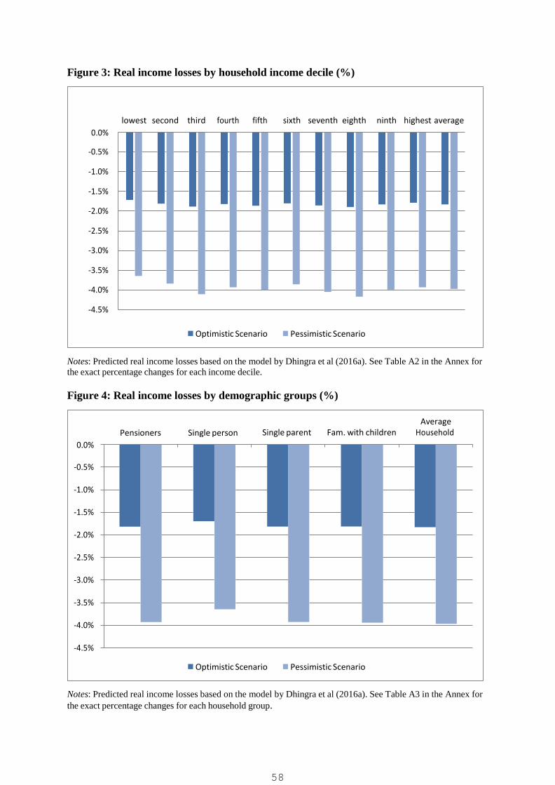
Figure 3: Real income losses by household income decile (%)

Notes: Predicted real income losses based on the model by Dhingra et al (2016a). See Table A2 in the Annex for

the exact percentage changes for each income decile.

Figure 4: Real income losses by demographic groups (%)


the exact percentage changes for each household group.

Pensioners Single person Average

Single parent Fam. with children Household

0.0%

-0.5%

-1.0%

-1.5%

-2.0%

-2.5%

-3.0%

-3.5%

-4.0%

-4.5%

Optimistic Scenario Pessimistic Scenario

lowest second third fourth fifth sixth seventh eighth ninth highest average

0.0%

-0.5%

-1.0%

-1.5%

-2.0%

-2.5%

-3.0%

-3.5%

-4.0%

-4.5%


58

The effects analysed so far are ‘static’, so they ignore the effects of trade on productivity as

well as the impact of Brexit on foreign direct investment (FDI), which is substantial.

Incorporating these effects more than triples the magnitude of the income losses, as

demonstrated in Dhingra et al (2016a). We illustrate this in Figure 5. We summarise the

equivalent figures in cash (2016 prices) as well as percentage terms in Table 1 with more

details in the Annex (Table A2). Note that these are all in terms of household gross income

(not GDP).

Figure 5: Long-run real income losses by household income decile (%)


the exact percentage changes for each income decile.

Looking solely at the static impact of trade, the income of the average UK household drops

by between 1.8% (£754) per year and 4% (£1,637) per year. If we take into account the

longer-run dynamic effects of Brexit on productivity, average households lose between 6.1%

and 13.5% per year of their real incomes per year (£2,519 to £5,573). For the poorest tenth of

households (bottom decile), real income losses are 1.7% to 3.6% in the short run and 5.7% to

12.5% in the long run. For the richest households, the short-run losses are 1.8% to 3.9% and

the long-run losses are 6% to 13.4%.

lowest second third fourth fifth sixth seventh eighth ninth highest average

0.0%

-2.0%

-4.0%

-6.0%

-8.0%

-10.0%

-12.0%

-14.0%

-16.0%


59

Table 1: Summary of distributional effects of Brexit in cash terms

Static Static Dynamic Dynamic

Optimistic Pessimistic Optimistic Pessimistic

(1) (2) (3) (4) (5) (6) (7) (8)

Group

Average

Gross

Income

% £ % £ % £ % £

Poorest

10% £10,019 -1.7% -£172 -3.6% -£365 -5.7% -£575 -12.5% -£1,248

Average £41,238 -1.8% -£754 -4.0% -£1,637 -6.1% -£2,519 -13.5% -£5,573

Richest

10% £110,228 -1.8% -£1,968 -3.9% -£4,329 -6.0% -£6,578 -13.4% -£14,744

Notes: 2015-16 gross incomes figures projected from ONS (2012, 2014). Optimistic is the EEA model and

Pessimistic is the WTO model. Dynamic model includes productivity effects of trade and FDI, static model does

not. Summarised version of Table A2 in Annex.

Incorporating other distributional effects of Brexit

The calculations so far focus on price changes and therefore the effects on real income,

implicitly assuming that nominal wage changes are proportional across income groups (that

is, the percentage changes are the same). This seems to be a reasonable assumption. The

changes in prices across sectors predicted by our model are not significantly correlated with

average skills (as measured by earnings) across sectors (Annex).

Economists for Brexit (2016) recommend that the UK unilaterally abolishes all trade barriers

after leaving the EU. They claim that this will increase UK trade and incomes. Their model

predicts extremely large increases in wage inequality, which would mean that lower income

groups would lose out much more from Brexit than we find. Dhingra et al (2016c) show that

the modelling approach used by Economists for Brexit is unreliable as it is inconsistent with

the most basic empirical evidence on how countries trade (for example, their model implies

that the UK could cease exporting to the EU entirely at no cost). When we examine the

impact of trading under WTO rules and moving unilaterally to free trade, the losses in real

income would still be substantial.

We do not model adjustment costs arising from the need to move workers across different

sectors because it is difficult to know what the exact effects would be. As there are likely to

be such adjustment costs from the Brexit shock, this would magnify the income losses

discussed here.

There is a view that EU immigration has had a negative effect on the labour market and that

Brexit would help this by reducing migration. But as Wadsworth et al (2016) show, EU

immigration has not increased unemployment or reduced the wages of the UK-born living in

the areas where immigration has risen the most. Nor is there any robust evidence that the

low-waged were hurt by much more than those at the top of the income ladder (Centre for

European Reform, 2016). In fact, the most likely impact of EU immigration on wages is a

60

positive one due to improved productivity. So it is unlikely that changes to immigration

patterns would materially alter the pattern of income losses reported here.

Conclusions

Economists consistently find that Brexit would lower real incomes in the UK. The cost of

lower trade and foreign investment would not be outweighed by a reduction in the net fiscal

transfer to other parts of the EU.

This report shows that the economic cost of Brexit would not be just born by the rich. The

pain would be evenly shared across the income distribution – every group would lose by

broadly similar proportions. Those in the middle would lose slightly more than others, with

average losses of between 1.8% (£754 per year) and 13.5% (£5,573 per year).

When it comes to the pain from leaving the EU, it appears that no one would be spared.

May 2016

For further information Contact: Holger Breinlich ([email protected]), Swati Dhingra

([email protected]) Thomas Sampson ([email protected]), John Van Reenen

([email protected]) or Romesh Vaitilingam ([email protected])

61






Further reading

Centre for European Reform (2016) The Economic Consequences of Leaving the EU

(https://www.cer.org.uk/publications/archive/report/2016/economic-consequences-leaving-

eu-final-report-cer-commission-brexit).

Dhingra, S., H. Huang, G. Ottaviano, J.P. Pessoa, T. Sampson and J. Van Reenen (2016a)

‘The Costs and Benefits of Leaving the EU: Trade Effects’, CEP

(http://cep.lse.ac.uk/pubs/download/brexit02_technical_paper.pdf).

Dhingra, S., G. Ottaviano, T. Sampson and J. Van Reenen (2016b) ‘The Consequences of

Brexit for UK Trade and Living Standards’, CEP Brexit Analysis No. 2

(http://cep.lse.ac.uk/pubs/download/brexit02.pdf).

Dhingra, S., G. Ottaviano, T. Sampson and J. Van Reenen (2016c) ‘Economists for Brexit: A

Critique’, CEP Brexit Analysis No. 6 (http://cep.lse.ac.uk/pubs/download/brexit06.pdf).

Economists for Brexit (2016a) ‘The Economy After Brexit’

(http://issuu.com/efbkl/docs/economists_for_brexit_-

_the_economy/1?e=24629146/35248609).

HM Treasury (2016) ‘The Long-term Economic Impact of EU Membership and the

Alternatives’, London: HMSO.

IFS (2016) ‘Brexit and the UK’s Public Finances’, Institute for Fiscal Studies.

NIESR (2016) ‘The Economic Consequences of Leaving the EU’, May Special Issue,

National Institute of Economic and Social Research.

OECD (2001) ‘COICOP-CPC and CPC-COICOP Correspondence Tables’, Paris.

OECD (2016) ‘The Economic Consequences of Brexit: A Taxing Decision’ Paris: OECD

http://www.oecd.org/economy/the-economic-consequences-of-brexit-a-taxing-decision.htm

ONS (2012), ‘Living Costs and Food Survey 2011,’ Office for National Statistics.

ONS (2014), ‘The Effects of Taxes and Benefits on Household Incomes 2013/2014,’ Office

for National Statistics.

ONS (2016), ‘Average weekly earnings by industry (EARN03),’ Office for National

Statistics.

Wadsworth, J. Dhingra, S., G. Ottaviano, and J. Van Reenen (2016) ‘Brexit and the Impact of

Immigration on the UK’, CEP Brexit Analysis No. 5


62

https://www.cer.org.uk/publications/archive/report/2016/economic-consequences-leaving-eu-final-report-cer-commission-brexit

https://www.cer.org.uk/publications/archive/report/2016/economic-consequences-leaving-eu-final-report-cer-commission-brexit

http://cep.lse.ac.uk/pubs/download/brexit02_technical_paper.pdf



http://issuu.com/efbkl/docs/economists_for_brexit_-



Annex: More details of the calculations

To calculate the implied effects of Brexit across the income distribution and different

demographic groups, we start with the estimated effects on industry prices from our structural

computable general equilibrium model in Dhingra et al (2016a). For different assumptions

over post-Brexit trading relationships, we estimate what effect this will have on industry

prices and average nominal wages. In our model, Brexit-induced price changes vary across

sectors for three reasons:

First, trade barriers increase by different amounts across sectors.

Second, a given increase in barriers will lead to different price changes in different

sectors, depending on how much of the trade cost change is passed on to consumers.

Third, all sectors use inputs from other sectors, so that they are also affected by

changing trade barriers in those other sectors through input-output relationships.

The end result of our model simulations is a list of price changes for each of the 31 sectors

from the World Input Output Data (WIOD), shown in Table A1 below.

Data for household expenditure on goods and services by income and demographic groups

are available from the 2012 edition of the Office for National Statistics (ONS) Living Costs

and Food Survey (Tables A5, A6 and A17). Figure 1 shows expenditures of each income

decile on 13 broad groups of final goods and services. We map the 31 WIOD sectors onto

these 13 expenditure groups using correspondences provided by OECD (2001). As explained

in the main text, households do not directly consume some of the intermediate input sectors

in WIOD (for example, basic metals such as steel) but are still affected by the corresponding

price changes as it feeds into the prices of final goods that they do buy (for example, cars).

Figure A2 shows the correlation between average weekly earnings by sector and the price

changes from Table A1. Average weekly earnings are from ONS (2016). The fitted line in

Figure A2 is based on an OLS regression of price changes on average weekly earnings. The

slope of the fitted line is 0.0009 and the corresponding robust standard error is 0.0013.

Because the slope coefficient is not statistically significantly different from zero, we assume

in our analysis that there is no differential impact of Brexit on nominal wages.

Table A2 gives the details on the exact proportionate losses by income groups and their cash

equivalents shown in the Figures and Table 1. We update the level of income from ONS

(2014), which has 2013-14 data to 2015-16 values using the growth in income of 5.2% over

the two years from ONS. Note that although the numbers are similar to those in Dhingra et al

(2016a) they are not identical for two main reasons.

First, we are looking at the effects on real incomes of final consumers. The average price

increase in Figure 1 is larger than in Table A1 because the effects of Brexit are greater on

prices of final goods and services that households directly spend money on (like food) than

they are for intermediate goods (like non-metallic minerals).

Second, we are looking at household income and spending rather than GDP (average GDP

per household is higher than average income per household). For example, households report

63

spending only small amounts on health and education as these are provided as free public

services by the state. Since the prices of health and education do not rise much, there appears

to be little negative effect on these items. This is why looking at overall GDP, which includes

government spending (as we did in Dhingra et al, 2016a), is in some respects preferable to

looking at just household spending and income patterns.

The long-run calculations are based on calculations in Dhingra et al (2016a). There we find a

long-run reduced form impact reduction of real GDP per capita of between 6.3% and 9.5%

compared with 1.3% (optimistic) and 2.6% (pessimistic) in the short-run static model. Using

the midpoint of the static effects (1.95%) and a conservative lower bound of 6.3% for the

dynamic effects, this implies a ratio of 3.23 (=6.3/1.95) between static and dynamic. We pro-

rata up the static effects by this ratio to calculate the dynamic effects in Figure 5.

Table A1: Price changes by product groups shown in Figure 1

Product group Optimistic scenario Pessimistic scenario

Food and non-alcoholic

drinks

3.1%

5.3%

Alcoholic drinks and tobacco 3.9% 7.2%

Clothing and footwear 2.1% 3.9%

Housing, fuel and power 0.8% 1.2%

Household goods and

services

1.6%

2.8%

Health 2.1% 3.8%

Transport 4.0% 7.7%

Communication 1.4% 2.6%

Recreation and culture 1.2% 2.1%

Education 0.0% 0.1%

Restaurants and hotels 0.7% 1.2%

Miscellaneous goods and

services

0.6%

1.1%

Other expenditure items 0.4% 0.8%

Notes: Table shows the exact price changes underlying Figure 1.

64

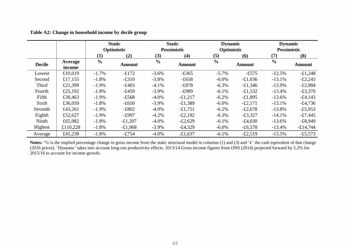
Table A2: Change in household income by decile group

Static

Optimistic

(1) (2)

Static

Pessimistic

(3) (4)

Dynamic

Optimistic

(5) (6)

Dynamic

Pessimistic

(7) (8)

Decile Average

income

% Amount

% Amount

% Amount

% Amount

Lowest £10,019 -1.7% -£172 -3.6% -£365 -5.7% -£575 -12.5% -£1,248

Second £17,155 -1.8% -£310 -3.8% -£658 -6.0% -£1,036 -13.1% -£2,243

Third £21,399 -1.9% -£403 -4.1% -£878 -6.3% -£1,346 -13.9% -£2,984

Fourth £25,192 -1.8% -£459 -3.9% -£989 -6.1% -£1,532 -13.4% -£3,370

Fifth £30,463 -1.9% -£568 -4.0% -£1,217 -6.2% -£1,895 -13.6% -£4,143

Sixth £36,059 -1.8% -£650 -3.9% -£1,389 -6.0% -£2,171 -13.1% -£4,736

Seventh £43,261 -1.9% -£802 -4.0% -£1,751 -6.2% -£2,678 -13.8% -£5,953

Eighth £52,627 -1.9% -£997 -4.2% -£2,192 -6.3% -£3,327 -14.1% -£7,445

Ninth £65,982 -1.8% -£1,207 -4.0% -£2,629 -6.1% -£4,030 -13.6% -£8,949

Highest £110,228 -1.8% -£1,968 -3.9% -£4,329 -6.0% -£6,578 -13.4% -£14,744

Average £41,238 -1.8% -£754 -4.0% -£1,637 -6.1% -£2,519 -13.5% -£5,573

Notes: ‘%’is the implied percentage change in gross income from the static structural model in columns (1) and (3) and ‘£’ the cash equivalent of that change

(2016 prices). ‘Dynamic’ takes into account long-run productivity effects. 2013/14 Gross income figures from ONS (2014) projected forward by 5.2% for

2015/16 to account for income growth.

65

Table A3: Change in household income by household groups (Figure 4)

Household group Pensioner Single person Single parent Families with

children

Optimistic scenario -1.8% -1.7% -1.8% -1.8%

Pessimistic scenario -3.9% -3.6% -3.9% -3.9%

Notes: Table shows the exact real income changes underlying Figure 4.

66

Table A4: Price changes by WIOD sector

WIOD31 Sectors Price

Change:

Optimistic

Price

Change:

Pessimistic

1 Agriculture, Hunting, Forestry and Fishing 1.60% 2.00%

2 Mining and Quarrying 2.10% 3.20%

3 Food, Beverages and Tobacco 4.20% 7.70%

4 Textiles and Textile Products; Leather, Leather and

Footwear 3.50% 5.10%

5 Wood and Products of Wood and Cork 1.60% 2.50%

6 Pulp, Paper, Paper , Printing and Publishing 1.60% 3.00%

7 Coke, Refined Petroleum and Nuclear Fuel 3.30% 3.80%

8 Chemicals and Chemical Products 6.30% 12.30%

9 Rubber and Plastics 2.50% 4.80%

10 Other Non-Metallic Mineral 1.40% 2.60%

11 Basic Metals and Fabricated Metal 3.70% 6.50%

12 Machinery, NEC (Not Elsewhere Classified) 4.20% 8.50%

13 Electrical and Optical Equipment 5.70% 10.10%

14 Transport Equipment 6.60% 13.90%

15 Manufacturing, NEC; Recycling 2.80% 5.20%

16 Electricity, Gas and Water Supply 0.10% 0.30%

17 construction 0.10% 0.20%

18 Retail Sale of Fuel; Wholesale Trade, Commission

Trade, including Motor Vehicles and Motorcycles 0.30% 0.60%

19 Retail Trade, Except for Motor Vehicles and

Motorcycles; Repair of Household Goods 0.10% 0.20%

20 Hotels and Restaurants 0.70% 1.20%

21 Inland Transport 0.30% 0.40%

22 Water Transport 1.70% 2.80%

23 Air Transport 2.50% 4.90%

24 Other Supporting and Auxiliary Transport Activities;

Activities of Travel Agencies 0.30% 0.50%

25 Post and Telecommunications 0.40% 0.70%

26 Financial Intermediation 0.50% 0.90%

27 Real Estate Activities 0.00% 0.10%

28 Other Business Activities and renting of equipment 1.50% 2.70%

29 Education 0.00% 0.10%

30 Health and Social Work 0.10% 0.10%

31 Public Admin, Defence, Social Security and other public

service 0.50% 1.00%

67

so

Single aren

.2

8

6

4

2

.1

8

6

4

2

0

Retired

Single per n

p t

Families with children

Chemicals

Engineering

Food & Drink

Metals Textiles

Other Manuf Mining

Agriculture

Transport

Hotels & Rest Public Sector Wholesale

Education Construction

600

Telecommunication Finance

Retail

200 400 800 1000 1200

Average Weekly Earning (£)

Figure A1: Spending shares on goods and services by demographic groups in the UK

0

0.1

0.1

0.1

0.1

0

0.0

0.0

0.0

0.0

Notes: Data from ONS (2012). Income deciles are based on gross household income.

Figure A2: Average sectoral earnings and Brexit-induced price changes

Notes: Average weekly earnings from ONS (2016), predicted price changes based on the model by

Dhingra et al (2016a).

4 6

0 2

68

The UK Treasury analysis of 'The long-term economic impact of EU membership and the alternatives':CEP Commentary

#CE

PB

RE

XIT

Swati Dhingra, Gianmarco Ottaviano,Thomas Sampson andJohn Van Reenen

BR

EXITP

AP

ER

The UK Treasury analysis of ‘The long-term economic

impact of EU membership and the alternatives’:

CEP Commentary

This week the UK Treasury released a much-discussed Report on the economic impact of the

UK leaving the EU. Their central estimate was a 6.2% fall in GDP (£4,300 per household).

We explain and analyse the Report and conclude it is a serious contribution to the Brexit

debate. Our major criticism is that the Treasury have been overly cautious in their assumptions

for their central case (a negotiated bilateral agreement, like the Canadian trade deal) and the

true long-run costs of Brexit are likely to be higher than they estimate.

The UK Treasury recently released an analysis of the long-run consequences of leaving the

European Union (EU) for the UK economy https://www.gov.uk/government/publications/hm-

treasury-analysis-the-long-term-economic-impact-of-eu-membership-and-the-alternatives.

The Report analyses the consequences of three different post-Brexit scenarios:

(i) The UK adopts the ‘Norwegian’ model and joins the European Economic Area

(EEA);

(ii) The UK adopts the ‘Canadian’ model and negotiates a Free Trade Agreement

(FTA) with the EU;

(iii) The UK trades with the EU under World Trade Organization (WTO) rules.

The Treasury’s analysis suggests that Brexit would lead to a long-run fall in UK GDP of 3.8%

under the Norway option, 6.2% under the Canada option and 7.5% under the WTO option.

But how did the Whitehall mandarins calculate these numbers? And should we believe them?

Roadmap to the Treasury analysis

The Treasury studies the long-run effects of Brexit using a three-step process:

Step 1: how Brexit would affect trade and foreign direct investment (FDI);

Step 2: how the reduction in trade and FDI following Brexit would affect productivity;

Step 3: the results of Steps 1 and 2 are combined with a global macroeconomic model

to predict how Brexit would affect overall UK national income.

We consider each of these steps in turn.

Step 1: How would Brexit affect trade and FDI?

A ‘gravity model’ is used to estimate how leaving the EU would affect the UK’s trade (separate

estimates are calculated for goods trade and services trade) and FDI. This gravity model

approach follows best practice in the academic literature and the Treasury’s estimates are

consistent with a large body of existing work. It is an empirical model relating data on the flows

of trade between all pairs of countries to the characteristics of these countries (for example,

their respective size as measured by GDP). For example, the bilateral goods data covers over

200 countries for the period 1948-2013 leading to the 390,521 observations in Table A.1. The

bilateral flows of service trade and FDI works in basically the same way.

70

https://www.gov.uk/government/publications/hm-treasury-analysis-the-long-term-economic-impact-of-eu-membership-and-the-alternatives

https://www.gov.uk/government/publications/hm-treasury-analysis-the-long-term-economic-impact-of-eu-membership-and-the-alternatives

The models focus only on changes over time, so lots of things like culture and distance between

countries are controlled for. Variables indicating whether or not two countries are in the EU

(or other FTAs or the EEA) are included in these models to estimate how much more EU

members trade with each other, after controlling for all the other determinants of trade or FDI.

In the ‘Canada’ case, the Treasury estimates that Brexit would reduce UK trade by up to 19%

(Table 3.A) and FDI inflows would fall by up to 20% (Table 3.B). This is how much trade

would fall by if, instead of being in the EU, the UK simply had a ‘deep’ FTA like the imminent

EU-Canada deal.

Step 2: How would Brexit affect productivity?

The effects of Brexit on UK productivity are obtained by combining the changes in trade and

FDI from Step 1 with estimates of how these changes affect productivity. Step 2 captures the

dynamic effects of Brexit on productivity. Estimating the exact relationship between trade or

FDI and productivity is tricky. For trade, the Treasury survey a range of estimates and settle

on those from Feyrer (2011), who finds elasticities of 0.2 to 0.3 – that is, a 10% fall in trade

reduces productivity by 2% to 3%.

For the impact of FDI on productivity, the literature is thinner than for trade so the Treasury

conduct original empirical analysis. They relate productivity at the broad industry level to the

level of the FDI stock. They find an elasticity of 0.04 – that is, a doubling of the FDI stock

raises productivity by 4%.

Step 3: How do these changes affect total GDP?

The changes in trade, FDI and productivity from Steps 1 and 2 are fed into a macroeconomic

model (NIESR’s NIGEM) to forecast the overall effects of Brexit on UK GDP. This final step

also incorporates several additional effects of Brexit.

First, the short-run shock of Brexit through uncertainty and other channels is likely to cause

some permanent loss of capacity. The Treasury assume this causes a 1% decline in GDP.

Although the idea that uncertainty and other negative shocks can have large and long-run

effects is reasonable (for example, Bloom, 2014), the precise magnitude of the persistence of

the shock is hard to judge.1

Second, the fall in productivity growth will have an impact on the aggregate capital stock,

which will also reduce GDP, and the macroeconomic model helps to pin this down. Third, the

macroeconomic model allows for complex interactions between trade, investment, prices, etc.

Step 3 is the least transparent part of the analysis as the macroeconomic model has a lot of

moving parts. It is difficult to incorporate all the elements in Steps 1-3. However, given the

reasonable desire to take a comprehensive view of many elements of the economic effects of

Brexit and allow for their interactions it seems a fair attempt.

Fortunately, it is not too hard to see how the various steps contribute to the overall decline in

GDP. It seems that most of the quantitative action comes from the effect of reduced trade on

1 The Treasury has said that a future report will provide greater detail on the short-run disruption resulting from

Brexit.

71

GDP, with a smaller contribution from FDI and the persistence of the shock. The

macroeconomic model itself in Step 3 plays a more minor role.

An illustration of the Treasury calculations

To illustrate how the numbers add up we give an example in Table 1 that shows how the

different steps contribute to the overall decline in GDP. We do this for the ‘upper end of the

negotiated bilateral agreement’ (for example, Canada) but the same logic applies to the other

cases considered.

The first row of Table 1 looks at trade effects and the second row looks at FDI effects. The

trade effects come from the gravity model comparing the coefficients on EU membership to

FTA membership (a weighted average over the goods and service regressions). This is a 19%

fall for trade (column 1). Column (2) is the effect of trade on GDP (0.3). Column (3) is simply

the first two columns multiplied together, which generates the overall fall in GDP because of

a Brexit induced trade loss of 5.7% (= 19% x 0.3).

Row 2 repeats the same analysis for FDI. The gravity model predicts a fall in FDI of 20%

(column (1)), which combined with the Treasury’s estimate of the FDI effect on productivity

of 0.04 (column (2)) leads to a 0.8% (= 20% x 0.04) fall in productivity in column (3).2

If we add the effects of trade (last column of row 1) and FDI (row 2) to the 1% fall of GDP due

to the persistence of the ‘Brexit shock’ (row 3), we get in row 4 a total of 7.5% fall of GDP (=

5.7% + 0.8% + 1.0%).

The Treasury Report calculates that the overall GDP loss after feeding all the effects into their

macroeconomic model is 7.8%. The additional 0.3% (=7.8% - 7.5%) loss of GDP in getting

from row 4 to row 5 is from the general equilibrium effects introduced by the macroeconomic

model. Exactly how their additional effects work through is not entirely clear. Part of it comes

from the endogenous response of the capital stock to lower productivity. Other parts may come

from interactions between various parts of the economy. Annex A goes into some more detail

on this.

2 The reason why the sum of the effects of trade and FDI is 6.5% = (5.7% + 0.8%) instead of the 6% given in the

middle column of the Treasury Report Table 3.C is basically to avoid double counting the effects of trade in the

macro-model. Feyrer’s (2011) estimates are trade effects on GDP so include a pure productivity effect plus an

effect on the capital stock. We explain this in Annex A.

72

Table 1:

How the Treasury arrives at their effects of Brexit on GDP- the example of the

‘upper end’ of the negotiated bilateral arrangement (‘Canadian model’)

(1) (2) (3)

Row 1: Trade Step 1: Brexit effect

on trade, Tables 3.A &

A.7

Effect of trade on GDP

(elasticity), Feyrer

(2011)

Step 2: Brexit

effect on GDP via

trade,

-19% 0.30 -5.7%

Row 2: FDI Step 1: Brexit effect

on FDI, Table 3.B

Effect of FDI on

productivity

(elasticity), Table A.14

Step 2: Brexit effect on

productivity via FDI

-20% 0.04 -0.8%

Row 3: Persistent effect of Brexit

disruption shock (1% of GDP)

-1%

Row 4: Sum of effects of trade, FDI &

persistence shock

-7.5%

Row 5: Overall Effect on GDP (Step

3), Table 3.D

-7.8%

Implied additional effects of

macroeconomic model

-0.3%

Notes: CEP analysis of how to think about the Treasury’s results.

73

The Treasury’s bottom line

An important point in all of this is that the main parts of the quantitative effects are not driven

by the less transparent macroeconomic model which only accounts for a small fraction of the

overall effect (0.3% of the 7.8% total effect). The majority of the impact is through easily

understood mechanisms of trade, FDI and the permanent effect on output from a big short-run

Brexit shock.

The second important point is that most of the magnitude of the effect is coming from the

impact of lower trade on productivity: (5.7% of the 7.8%).

Similar calculations can be made for the ‘lower end of the range’ negotiated bilateral

arrangement. In this case, the fall in trade is only 14%3 (instead of 19%), the fall in FDI only

15%4 (instead of 20%) and the effect of trade on GDP reduced to 0.2 (instead of 0.3). Putting

all these together with the transition shock leads to a total of 4.4% (= 2.8% + 0.6% + 1%). If

compared to the Treasury Report’s final number of 4.6% in Table 3.D, the implication is that

the macroeconomic model adds another 0.2% of GDP to the cost. Again, Step 3 is

quantitatively small and trade effects are the largest component of the overall effect.

The headline number of a loss of 6.2% of GDP is the simple average of the lower end and

upper end estimates (i.e. = (7.8% + 4.6%)/2).

The main problem of the Treasury Report: too cautious by half?

The Treasury analysis has been criticised by some for being deliberately designed to generate

very large negative effects of Brexit. This criticism is off the mark. The assumptions and

analysis are all explicitly stated and economically reasonable. Different people will have

different views of which of the three trading arrangements is most likely after negotiations with

the EU are complete, but the analysis lays out the economic consequences of the possible

options. The 15-year horizon is sensible since such negotiations are usually extremely

protracted.

In fact, our view is that the Treasury have been too conservative in many of their assumptions

and should have generated larger effects. The following are some examples of their cautious

approach.

The impact of Brexit on the loss of trade and FDI

The Treasury’s ‘lower end’ estimates assume some of the benefits of EU membership are

‘banked’ and will remain, even 15 years after the UK leaves the EU. For example, in our Table

1, their lower end estimates are of a case where trade and FDI fall substantially less than their

empirical estimates suggest (they use 14% instead of 19% for trade and 15% instead of 20%

for FDI). There is no obvious reason to do this, apart from wanting to be very cautious.

3 Middle column of Table 3.A. 4 Middle column of Table 3.B.

74

The impact of trade on productivity

The Feyrer (2011) elasticity of 0.2 to 0.3 is conservative. This paper uses the fall in trade costs

due to the closure of the Suez Canal as a natural experiment. But Feyrer (2011) only looks at

the effects over an eight year horizon, whereas the long-run horizon the Treasury is considering

is 15 years, leading to larger dynamic effects.

A better study to use would have been Feyrer (2009) that looks over a longer period using

multiple natural experiments of falls in transport costs. This paper finds elasticities of 0.5 to

0.75 – over twice as large as those used by the Treasury. One reason for the Treasury’s more

cautious approach is that these elasticities might include some FDI component that they want

to model separately. But this seems excessively cautious as FDI flows were not so important

during the time period for which the trade elasticity is estimated (Feyrer, 2011, ends in 1975).

The impact of FDI on productivity

The approach used by the Treasury may also underestimate the benefits from FDI. First, the

industry level data used to estimate the FDI elasticity may miss out on some of the cross-

industry productivity effects that the literature has stressed (e.g. across supply chains and from

learning). Second, the use of UK only data with time trends may reduce a lot of the useful

variation in FDI, making - and so underestimating - the positive effects on productivity. This

is suggested by the fact that dropping the industry trends doubles the impact of FDI on

productivity (first column of Table A.14).

An alternative, using cross country data over time, is Alfaro et al (2004) whose model captures

more of the cross industry benefits of FDI. We use this in Dhingra et al (2016b) which implies

much larger impacts of FDI on GDP, as does the earlier work of Pain and Young (2004).

Continuing reductions in trade costs within the EU

The Treasury Report assumes that there is no further integration within the EU to reduce trade

costs. But one section of the Report does look at this and suggests that it would add up to

another 4% of GDP (paragraph 3.89). It seems highly likely that there will be further reductions

in non-tariff barriers within te EU, especially in services, which is critical to the UK economy.

Over the last 50 years there has been an on-going process of reductions in within EU trade

costs, so assuming this suddenly comes to a juddering halt is unduly pessimistic.

In Dhingra et al (2016a), we model this by considering whether falls in trade costs within the

EU continue along their historical trend (business as usual) or slow down to half the historical

rates. This seems a more likely scenario than the baseline considered by the Treasury.

Immigration

The Report uses ONS projections of migration. This does not affect the results in any material

way as they are on a per capita. The Treasury are essentially assuming no impact of migration

on productivity. This is again rather cautious as most economists find positive effects of

immigration on aggregate income per head, especially since EU migrants are more educated

and younger than the UK-born (http://www.niesr.ac.uk/blog/treasurys-brexit-analysis-and-

immigration#.VxiKaE32aUn).

75

http://www.niesr.ac.uk/blog/treasurys-brexit-analysis-and-immigration#.VxiKaE32aUn

http://www.niesr.ac.uk/blog/treasurys-brexit-analysis-and-immigration#.VxiKaE32aUn

Other criticisms of the Treasury Report

Is forecasting so far out impossible?

Many ‘Leave’ commentators have attacked the Report by saying it is impossible to forecast

events so far in the future. Although the Report is pitched as what will be GDP in 15 years’

time, it is important to realise that this is an analysis rather than a forecast. The Report is in

essence saying how much poorer the UK is likely to be because of Brexit. Current forecasts of

the global economy could be too pessimistic as technological change may pick up. Or they

might be too optimistic if China has a debt meltdown. But whatever happens, we can consider

what will be the state of the UK economy relative to these outcomes. And the Report is

essentially saying that whatever unexpected events happen in the world, the UK is likely be

considerably poorer than it would have been if it remained in the EU.

Fiscal transfer

The Report does not focus on net fiscal transfers to the EU. As we argue in Dhingra et al

(2016a), these are not likely to be large enough to outweigh the economic losses as the transfer

is about 0.31% of GDP. In the case of the EEA, there is likely to be a continued large transfer

(Norway pays in 88% of what the UK does on a per capita basis) and similarly large transfers

are made even in looser arrangements (for example, 40% in the Swiss case).

Benefits of cutting ‘red tape’

The Report argues there is unlikely to be much of an effect from changes in regulation

following Brexit, as the UK is already one of the most lightly regulated countries in the

developed world. This is the same conclusion that we reach in Dhingra et al (2016a).

Although the UK Government’s Impact Assessment finds that the benefits of most regulations

derived from EU laws have outweighed their costs, Booth et al (2015) point to 56 regulations

where costs outweigh the benefits. Crafts (2016) estimates that the cost of these regulations is

0.9% of the UK’s GDP. But many of these regulations implement policies that the UK

government is committed to following inside or outside the EU. For example, half of the total

cost comes from just two policies: the Renewable Energy Strategy; and the Working Time

Directive. Scrapping these regulations would mean abandoning the UK’s renewable energy

targets and removing rights such as the entitlement to 20 days paid annual leave. And even if

the regulatory costs of EU membership were 0.9% of GDP and there was the political will to

abolish these regulations, this figure is substantially smaller than the GDP decline forecast in

the Report.

‘Look globally and strike great trade deals’

Another criticism is that the document ignores the possibility that after Brexit, the UK will re-

orient its trade towards faster-growing economies such as China, India and the United States.

The UK actively promote trade with these countries now, but it cannot strike trade deals with

them alone.

When negotiating post-Brexit trade deals, the UK would not need to compromise with other

EU countries. On the other hand, the UK would have to take on the cost of hiring civil servants

to rebuild its capacity to undertake trade negotiations which can take decades. More

76

importantly, since the UK is under a fifth of the economic size of the EU Single Market it

would have less bargaining power in trade negotiations than the EU does. And being outside

the EU would mean it no longer automatically accessed the benefits from the EU’s trade deals,

such as the current ones being negotiated with the US and Japan worth around 0.6% of GDP.

It beggars belief that these putative trade deals would be on so much better terms than the

existing and future deals that the EU has negotiated, that they would outweigh the larger loss

of trade and investment identified in the Report.

‘Leaving the EU will shield us from its decline’

Some critics believe that the EU is about to collapse and the UK will be shielded from the fall

out by jumping from the sinking ship. It is true that the EU (like the UK) has become a smaller

part of the world economy over the last two decades. But this is not because the EU has not

grown – it has simply not grown as fast as the rising economies such as China or India. Given

the geographical fact that we are a neighbour to Europe, developments in the EU block will

always have a major effect on the UK. Throwing up masses of trade barriers with the EU (which

Brexit supporters claim they will not do) will ‘shield’ us only in the sense it would decouple

us from our major economic partners.

Conclusions

Forecasting the economic consequences of Brexit is a difficult challenge and all estimates will

be subject to a degree of uncertainty. But our overall assessment is that the Treasury Report is

a credible analysis, which, for the most part, uses the best available estimation methods. Our

main criticism is that they have taken overly cautious assumptions which will tend to

underestimate the economic costs of Brexit.

Their headline forecast that Brexit would reduce long-run UK GDP by 6.2% in the baseline

case is broadly consistent with our previous work and many other independent estimates. For

example, in Dhingra et al (2016a), our dynamic estimates of the cost of Brexit indicate a GDP

loss of 6.3% to 9.5% in the case of moving from the EU to EFTA (see Annex B). Treasury

estimates are at the lower end of this range.

The Treasury’s findings reinforce the academic and business consensus that Brexit would make

the UK significantly poorer. The Report is a serious contribution to the debate.

77

Further Reading

Alfaro, L., A. Chanda, S. Kalemli-Ozcan and S. Sayek (2004) ‘FDI and Economic Growth:

The Role of Local Financial Markets’, Journal of International Economics 64(1): 89-112.

Bloom, N. (2014) ‘Fluctuations in Uncertainty’, Journal of Economic Perspectives 28(2) 153-

76.

Booth, S., C. Howarth, M. Persson, R. Ruparel and P. Swidlicki (2015) ‘What If..? The

Consequences, Challenges and Opportunities facing Britain outside the EU’, London: Open

Europe.

Crafts, N. (2016) ‘The Growth Effects of EU Membership for the UK: A Review of the

Evidence’, University of Warwick mimeo.

Dhingra, S., G. Ottaviano, T. Sampson and J. Van Reenen (2016a) ‘The Consequences of



Dhingra, S., G. Ottaviano, T. Sampson and J. Van Reenen (2016b) ‘The Impact of Brexit on

Foreign Investment in the UK’, CEP Brexit Analysis No. 3


Feyrer, J. (2009) ‘Trade and Income – Exploiting Time Series in Geography’, NBER Working

Paper No. 14910.

Feyrer, J. (2011) ‘Distance, Trade and Income – The 1967 to 1975 Closing of the Suez Canal

as a Natural Experiment’, NBER Working Paper No. 15557.

Pain, N. and G. Young (2004) ‘The Macroeconomic Effect of UK Withdrawal from the EU’,

Economic Modelling 21: 387-408.

78



Annex A: How the macroeconomic model affects the results

In NIESR’s NIGEM macroeconomic model the Treasury simulate for each of their scenarios:

A shock to the size of the ‘Rest of World’, which reduces trade on par with the fall

assumed in the relevant scenario.

A fall in labour augmenting technical change equivalent to the impact from trade and

FDI estimated in each scenario.

The macroeconomic model then calculates the long-run changes in GDP, prices, etc. These are

compared to the baseline case without these shocks (i.e. the case if the UK stayed in the EU).

One tricky issue is the size of the technology shock. Consider our example in Table 1 of the

upper end of the case of the negotiated bilateral agreement (Canada). An obvious strategy

would be simply to use the implied productivity effect of -5.7% in Table 1 (column (3) of row

1). However, this would imply some ‘double counting’, as Feyrer’s (2011) estimates of the

impact of trade changes on income already include productivity increases due to endogenous

increases in the capital stock that trade induces.

The Treasury’s solution is to figure out what is the size of the productivity/technology shock

necessary to generate a change of GDP equal to 5.7%. They do this by using the NIGEM model

and the assumed change in exports (or its equivalent in a shrinkage of the exporter market size).

It turns out that the implied magnitude of the technology shock is 5.2%.5 They then add the

productivity impact of FDI to get to a total technology shock of 6% (5.2% + 0.8%) They then

add this shock of 6% into the NIGEM model alongside the trade shock to simulate the new

level of GDP and other macro-economic outcomes.

5 We can tell this because Table 3.C indicates that a 6% technology shock has been fed into the NIGEM model,

and the impact of FDI on productivity is 0.8% in our Table 1 (see column (3) of row 2). So 5.2% = 6.0% - 0.8%.

79

Annex B: How the Treasury Report relates to our own estimates

The closest calculation that is comparable is the dynamic reduced form approach in Dhingra et

al (2016a). There we find a 12.5% fall in trade after Brexit from a free trade agreement (like

the Canadian case or EFTA). So this is similar to the Treasury’s ‘lower end’ estimate of 14%.

We use a higher GDP-trade elasticity from Feyrer (2009) of 0.5 to 0.75, which gives us a 6.3%

to 9.5% GDP loss. These also probably include some FDI response.

The Treasury’s baseline 6.2% GDP loss is at the lower end of these range of estimates.

The focus of Dhingra et al (2016a) is on static estimates from the costs of trade using a

structural model. This finds smaller losses of GDP of between 1.3% and 2.6%. This is a very

different methodology to the Treasury approach. In particular, it does not consider the dynamic

effects of trade on productivity. In addition it does not consider the effects of FDI or

immigration. In Dhingra et al (2016b) we take a simpler approach to looking at the effects of

FDI and find that Brexit would cause a 3.4% loss of GDP if we moved into EFTA.

80

Economists for Brexit: A Critique

Thomas Sampson, Swati Dhingra, Gianmarco Ottaviano and John Van Reenen

#CE

PB

RE

XIT

BR

EXITP

AP

ER

Introduction

Much publicity recently surrounded ‘Economists for Brexit’ (2016a, 2016b). Since the

economic case for leaving the European Union (EU) has been largely missing in action, it is

refreshing to obtain some clarity over the Leave campaign’s vision of the UK’s post-Brexit

economic arrangements.

Professor Patrick Minford of Cardiff University is the only one of the group who has provided

some economic modelling. He predicts that there would be a welfare gain of 4% of GDP by

2020 if the UK were to leave the EU. This prediction is surprising because just about every

other piece of economic analysis finds negative economic effects from the UK leaving the EU

(for example, Dhingra et al, 2016a; HM Treasury, 2016; NIESR, 2016; OECD, 2016; PWC,

2016).

Such studies simply remind people that the EU has been good for trade and trade is good for

welfare. It follows that leaving the EU will reduce trade and so have an economic cost. The

main question is not so much the direction of the effect, but rather the magnitude of the hit to

living standards. There may be offsetting or reinforcing factors from other things – such as

regulation, foreign investment, immigration, lower fiscal transfers to Brussels, uncertainty and

so on – but distancing ourselves from our closest trading partner could not be beneficial for

trade.

Yet Economists for Brexit make just such a claim, so we were curious to understand where

Minford’s positive effects come from. We summarise the main points of our analysis here and

leave more technical details to the Annex.

‘Britain Alone’ – unilateral free trade

One feature of Minford’s approach is that after leaving the EU, the UK is assumed to trade

simply under World Trade Organization (WTO) rules, without seeking a new trade agreement

with the EU or other trading partners like the United States. The UK would simply pay the

external tariffs. This is usually the worst case scenario that other economists have modelled.

HM Treasury (2016), for example, finds a GDP drop of 7.5% under this scenario.

A second feature of the Minford argument is the assumption that the UK will unilaterally drop

all its trade protection against imports from everywhere else in the world after Brexit. One

reason why most economists have not focused on this scenario is that it seems politically

unlikely. As far as we know, no developed country has ever unilaterally removed all

manufacturing tariffs against all other countries – Minford’s ‘Britain Alone’ scenario.

In fact, one can easily imagine the UK establishing greater trade protection after Brexit. For

example, the recent furore over Port Talbot’s steelworks suggests that domestic political

pressures may have pushed the government to increase tariffs on Chinese steel. Indeed,

Minford describes in his model that an implication of the ‘Britain Alone’ policy (Minford et

al, 2016, p. 74 Table 4.3) is that it will ‘effectively eliminate manufacturing’ in the UK. Another

implication of his preferred policy is a dramatic increase in wage inequality: skilled workers’

nominal wages increase by around 11%, but unskilled workers’ wages fall by 14%.1 These

changes are unlikely to be an easy sell politically, to say the least.

1 These inequality changes will not be offset by reductions in EU immigration as the impact of immigration on

inequality is close to zero (Wadsworth et al, 2016).

82

Nonetheless, standard economics does suggest that there will be some benefits from ‘unilateral

trade disarmament’. Indeed, in the work we published in March (Dhingra et al, 2016a, Table

2) we look at what would happen if the UK eliminated all tariffs after Brexit.2 We find that if

the UK trades under WTO rules following Brexit, but maintains import tariffs, then UK income

per capita falls by 2.6%. Under Minford’s ‘Britain Alone’ scenario of unilateral liberalisation

after Brexit only, UK real incomes still fall by 2.3%. In other words, there is a gain of only 0.3

percentage points from eliminating tariffs compared to just trading under WTO rules – this is

completely insufficient to offset the other trade costs of Brexit.

So the real question is not whether moving to unilateral free trade can have some benefits in

economic models, but rather:

Why the benefits are so big in Minford’s model (over ten times what we find)?

Why are there no welfare costs in Minford’s model from lower UK exports to the EU

after Brexit?

The answers to these questions require an understanding of how thinking about the economics

of trade has developed in the last five decades, and how these features are overlooked in the

Minford approach.

The basic idea

There are basically two steps in Minford’s analysis. First, he assumes that because of EU tariff

and non-tariff barriers, prices paid by UK consumers for manufacturing and agricultural goods

would fall by 10% under his ‘Britain Alone’ policy recommendation. Second, he feeds this

10% tariff equivalent fall in trade costs into his ‘Liverpool model’ to come up with a GDP

increase of 4% (roughly speaking, the increase in GDP is much less than 10% because people

consume a lot of services, which are not directly affected by Brexit under Minford’s

assumptions).

The 10% fall in trade costs

How on earth can trade costs fall by 10% when the UK’s average tariff is currently around 3%?

The answer is that the 10% number does not come from looking at the actual level of tariffs. It

comes from looking at the differences in price levels between the UK and some other countries

and arguing that these higher prices are due to protectionism caused mainly by EU regulations

(non-tariff barriers).

We go through this in detail in the Annex, but there are several very basic problems. First, the

estimates he makes are from data in 2002 - 14 years out of date.

Second, it seems extraordinarily unlikely that all the cross-country price differences are really

from trade protection rather than a multitude of other factors, such as quality differences,

variation in producer mark-ups or measurement error in estimates of distribution margins. For

example, say Europeans put a higher premium on high-quality clothing compared with

Americans. It will look like Europeans are paying more for their clothes, but in reality, the

higher average prices simply reflect a different mix of purchases – we are comparing apples

2 Mr. Minford is under the misapprehension that we did not look at his ‘Britain Alone’ recommendation, but this

is because he only refers to the work from two years ago (Ottaviano et al, 2014) and not the recent work (for

example, Dhingra et al, 2016a).

83

with oranges across countries (Deaton, 2015)4 Minford attributes these price differences to

nefarious EU regulation excluding cheaper clothing, whereas in fact it could reflect different

tastes for quality.

It is true that regulations could mean that prices are higher in the EU as there are stricter quality

controls than in other countries. The EU has tougher regulations over children’s milk and toys

than China does, so sub-standard products cannot be sold. This does create a trade barrier with

China and in Minford’s data a children’s toy will appear as identical, but more expensive in

the EU. But this reflects a quality difference. It is true that if the UK left the EU and relaxed

the safety standards down to China’s level prices would fall. But quality-adjusted prices would

not, and this is what is relevant for consumer welfare.

Third, Minford misunderstands the nature of regulations and product standards. The idea of the

Single Market is to have common rules so that a product sold in one EU country can also be

sold in any other. If there are 28 different sets of rules governing the sale of a product, it will

be harder to sell this product across all EU countries. The basic misconception in Minford’s

world is that the harmonisation of regulations between EU countries to reduce trade barriers is

simply a pernicious plot by vested interests to raise prices. In fact, playing by a common set of

rules is what helps increase trade and competition in a modern economy. Modern trade

agreements are hard because countries are trying to agree on common standards and to

harmonise rules that are different.

Minford overestimates the scope for reducing trade costs through unilateral liberalisation. In

our analysis of unilateral liberalisation, we focus on the removal of import tariffs because tariffs

are measurable and, in the event of Brexit, could be removed at the stroke of a pen.

One way to align standards is simply by co-ordinating on one rule or another; there is no better

or worse, weaker or stronger. But it takes two to tango. There simply is no way of unilaterally

aligning these type of standards. If the UK simply goes its own way on its own regulatory

standards, then this will increase the costs of trading with European countries and reduce the

amount of trade.

Other forms of harmonising rules require explicit agreement on how ‘tough’ a product standard

must be. Consider safety standards for children’s toys. Some countries may have very relaxed

standards over toy safety, but others may have very high standards. Let’s say the EU settles on

a standard for toys that is tougher than the UK would unilaterally choose, but weaker than

Germany would like.3 The single standard means that all manufacturers know that so long as

they meet the safety requirements, they can sell toys anywhere in the EU.

The high product standard is annoying for UK toy manufacturers, some of whom will now

have to comply with the EU Toy Safety Directive, even when they do not export to the EU.

They will complain that it’s only exporters that should have to comply with the higher EU

safety standards, as most Britons don’t care. But if the UK gets an ‘opt out’ to produce low

safety toys for domestic consumption, it means that there isn’t a level playing field – every

country will want an opt-out to decrease or increase the standard.

3 There are many other examples of such regulations – see Springford (2016). Examples include powdered milk:

http://eur-lex.europa.eu/LexUriServ/LexUriServ.do?uri=OJ:L:2007:258:0027:0028:EN:PDF; levels of arsenic

found in rice products for children:

https://www.food.gov.uk/enforcement/regulation/europeleg/euupdates/january-update-maximum-limits-for-

arsenic; and of course the classic case on lawnmower noise: https://next.ft.com/content/ac04efc8-34c8-11e3-

a13a-00144feab7de.

84

http://eur-lex.europa.eu/LexUriServ/LexUriServ.do?uri=OJ:L:2007:258:0027:0028:EN:PDF

https://www.food.gov.uk/enforcement/regulation/europeleg/euupdates/january-update-maximum-limits-for-arsenic

https://www.food.gov.uk/enforcement/regulation/europeleg/euupdates/january-update-maximum-limits-for-arsenic

https://next.ft.com/content/ac04efc8-34c8-11e3-a13a-00144feab7de

https://next.ft.com/content/ac04efc8-34c8-11e3-a13a-00144feab7de

In our example, the UK can sell high quality safe toys to Germany, but German toy

manufacturers can’t sell lower quality products to the UK as they are banned from producing

them. This is not just a political problem. UK consumers are worse off because locking out

foreign competition means that they face higher prices and less innovation.

Another practical problem with multiple standards is that with complex supply chains,

countries may not want to import from others with lax standards solely for domestic

consumption as it might contaminate the entire batch. This is why the EU and even the United

States want to have a global standard for toy safety (http://uk.reuters.com/article/health-toys-

safety-rules-dc-idUKL0889219620071108?pageNumber=1).

In this context, Minford’s ‘Britain Alone’ proposal would be that we leave the EU and lower

product standards. It is certainly possible for the UK to adopt the lowest standards unilaterally.

There would then be lower average prices and quality for children’s toys in the UK. But even

if this was what the British people wanted, the rest of the EU would not continue to grant the

same access to the Single Market as EU toy manufacturers would be excluded from part of the

UK market because of higher EU standards. This is why the EU insists that countries play by

the same rules if they want to be in the Single Market.

How Minford defies the laws of gravity

The gravity equation is the most reliable empirical relationship in international economics.

First estimated by Nobel laureate Jan Tinbergen, it shows that the trade flow between any pair

of countries increases as the economic size of the countries grows, and decreases with rising

costs of trade between them caused by import tariffs, transport costs and other trade barriers.

Geography matters – the further apart countries are, the less they trade. There are literally

hundreds of data-based studies showing the robustness of this relationship across many

countries, industries, time periods and multiple specifications (see Head and Mayer, 2014, for

a survey).

Today, the gravity equation is central to how economists understand international trade. It is a

key economic relationship, which performs extremely well in predicting actual trade flows. To

evaluate the effects of changes in trade policy, new methods have been developed that both

explain why trade follows a gravity equation and takes into account all the general equilibrium

effects of changes in trade policy on prices, wages and output in a multi-country, multi-industry

world with trade in both final goods and intermediate inputs.4

This matters because the analysis undertaken by Minford uses an old trade model in which all

firms in an industry everywhere in the world produce the same goods and competition is perfect

so that trade does not follow the gravity equation. This choice is largely responsible for why

Minford’s findings contradict the results of numerous other studies that conclude Brexit would

lower UK GDP.

How does his analysis work? With perfect competition and homogeneous products, the EU’s

tariffs and other regulations raise the price of imports and all other goods sold in the EU above

the free trade price. Therefore, if the UK leaves the EU and simultaneously removes all tariffs

and non-tariff barriers, prices fall, making the average UK consumer better off.

4 We use such a model to analyse the consequences of Brexit in Dhingra et al (2016a), which builds on Ottaviano

et al (2014). Minford (2016) is mistaken in thinking that general equilibrium effects are missing from this analysis.

They are not missing; they are just incorporated into a richer (but more transparent) model than the one he uses.

85

http://uk.reuters.com/article/health-toys-safety-rules-dc-idUKL0889219620071108?pageNumber=1

http://uk.reuters.com/article/health-toys-safety-rules-dc-idUKL0889219620071108?pageNumber=1

The problems with this analysis stem from the assumption that all firms in an industry produce

the same product. There are two main limitations with Minford’s model:

1. Exporters sell all their output at world prices. In reality, exporters sell their output in many

countries and face different trade barriers in each market. In Minford’s model, following

Brexit exporters sell all their output in a fictional world market. Consequently, the level of

trade barriers with the EU after Brexit does not matter to exporters as they do not care

whether trade goes to the EU or elsewhere. This feature of the model gets rid of the costs

of Brexit from reduced access to the EU market. In reality, as our geographically closest

neighbour, we will continue to trade with the EU. Brexit increases trade costs with the EU

and this causes us to trade less with them. We cannot just sell everything to the rest of the

world at the same price to make up for this loss. This is the primary cost of Brexit, but it is

absent from Minford’s model.

2. Both imports and domestic output have the same price. Therefore, the decline in import

prices when the UK removes import tariffs leads to an equal fall in domestic prices. In the

real world, domestic and foreign firms produce differentiated products, so a fall in import

prices will reduce domestic prices to a smaller extent and the benefits from unilateral trade

liberalisation are much smaller.

Comparing Minford’s approach with modern trade models

As noted in Dhingra et al (2016a, Table 2), we analyse the consequences of unilateral trade

liberalisation following Brexit in a modern general equilibrium trade model that is consistent

with the gravity equation. In this experiment, we continue to assume perfect competition, but

allow for product differentiation. This means that there is not perfect substitution between the

products of any given industry and thus the cheapest source country of a product is not

necessarily the best source country of all products in the industry. Our model also allows for

varieties of the same product to be sourced from different countries as consistent with different

consumer tastes.

Under Minford’s assumption that the UK trades simply under WTO rules and unilaterally

removes all import tariffs, we find that the Brexit effect is equivalent to a 2.3% decline in UK

income per capita. We conclude that Brexit would reduce UK living standards even if the UK

unilaterally sets all import tariffs to zero.

We also consider what happens if the UK falls back on general WTO rules and imposes the

EU’s current ‘most-favoured nation’ tariffs following Brexit. In this case, Brexit is equivalent

to a 2.6% decline in UK income per capita. Thus, Minford is right that there are benefits from

removing import tariffs, but these benefits are around 0.3 percentage points – much smaller

than the costs of Brexit resulting from increased trade costs with the EU.

In addition to satisfying the gravity equation, our model predicts that EU membership is trade-

creating, which means that it increases the UK’s trade. By contrast, Minford’s model is hard-

wired to predict that EU membership is only trade-diverting and Brexit would lead to higher

trade.

Our work and that of the other economic studies relies on data that show what has actually

happened to trade after joining the EU, rather than just asserting what should happen in a

theoretically dubious model.

The empirical research literature supports the conclusion that EU membership is trade-creating.

For example, Baier et al (2008) find that goods trade between EU members is 62% higher than

86

trade between otherwise comparable countries that have no trade agreement between them.5

Using more recent data, HM Treasury (2016) finds that EU membership raises intra-EU goods

trade by an even larger 115% relative to WTO membership.

There is little evidence that regional trade agreements lead to substantial trade diversion – see

the recent reviews by Bagwell et al (2014) and Limão (2016). For example, Magee (2008,

2016) finds no evidence of trade diversion from economic integration agreements. Consistent

with this evidence, HM Treasury (2016) finds no significant evidence of trade diversion

because of the EU.

Services

Services exports to the EU accounted for 16% of all UK exports in 2014 (ONS, 2015). UK

services exporters benefit from lower trade barriers with the EU resulting from the Single

Market. In particular, financial services firms can undertake business throughout the EU under

the EU’s ‘passporting’ rules. These rights would be lost if the UK left the Single Market.

Minford does not take this into account.

Foreign investment

Membership of the EU increases foreign direct investment (FDI) in the UK, which raises

productivity and output (Dhingra et al, 2016b). Minford argues that there are no benefits from

FDI, whereas the evidence points in the opposite direction. His views seem to be based on the

fact that the empirical estimates are ‘insecure’ (Minford, 2016) without saying why.

The role of empirical evidence in Minford’s world

Minford’s style of work was popular in some quarters in the 1970s. In those days, economics

did not need to be well-grounded in facts and data, and could rely on highly simplified theories.

The revolution over the last 40 years has been the explosion of data and empirical techniques

for its analysis. Good theory has evolved in tandem with this new evidence.

Theoretical foundations, ranging from Ricardian comparative advantage to modern product

differentiation models of imperfect competition, explain why the gravity model describes

international trade flows (for example, Head and Mayer, 2014). The approach that we use in

Dhingra (2016a) is to employ a model consistent with the basic facts of trade. It is a computable

general equilibrium model and well-grounded in theory. The difference between our approach

and Minford’s is that the theories we use are based on the facts of life in trade, such as the

gravity relationship, whereas his theory is unhinged from the most basic features of trade

reality.

Minford’s attitude seems to be that if empirical work is imperfect, it should be ignored. The

voluminous evidence on the positive impact of the EU on trade is dismissed because of

statistical concerns (Economists for Brexit, 2016b, p.20). Of course there are issues with all

empirical work. Some of these problems might mean we over-estimate the EU’s effect on trade

and FDI; some might mean we under-estimate it.

5 This estimate comes from Table 6, column 1 of Baier et al (2008) where 62% = e0.48 – 1.

87

But to take the position that since no econometric work can be perfect, all inconvenient facts

should be ignored is poor scholarship and bad science.

Conclusions

Alternative economic models have different advantages and drawbacks and are suited for

different purposes. Unfortunately, Minford’s model is inconsistent with two basic facts about

international trade; first that trade satisfies the gravity equation; and second, that the EU has

been trade-creating, not simply a tool for trade diversion.

Consequently, Minford’s model is not the right tool to use for predicting the consequences of

Brexit for trade and living standards. When we analyse the same scenario considered by

Minford using modern economics that incorporate advances in our understanding of

international trade data since the 1960s and a more realistic assessment of how UK ‘unilateral

trade liberalisation’ could actually work, we find (alongside just about everyone else) that

Brexit leads to a decline in UK living standards.

88

Further reading

Baier, S.L., J.H. Bergstrand, P. Egger and P.A. McLaughlin (2008) ‘Do Economic Integration

Agreements Actually Work? Issues in Understanding the Causes and Consequences of the

Growth of Regionalism’, The World Economy 31(4): 461-97.

Bagwell, K., C. Brown and R. Staiger (2014) ‘Is the WTO Passé?’ Stanford mimeo

(http://www.dartmouth.edu/~rstaiger/JEL_WTO_BBS_Draft_111014.pdf).

Bradford, S. (2003) ‘Paying the Price: Final Goods Protection in OECD countries’, Review of

Economics and Statistics 85(1): 24-37.

Deaton, A. (2014) ‘Getting Prices Right: The Mysteries of the Index’, LSE Lionel Robbins

Memorial Lectures

(http://www.lse.ac.uk/publicEvents/events/2014/12/20141210t1830vOT.aspx).

Dhingra, S., G. Ottaviano, T. Sampson and J. Van Reenen (2016a) ‘The Consequences of



Dhingra, S., G. Ottaviano, T. Sampson and J. Van Reenen (2016b) ‘The Impact of Brexit on

Foreign Investment in the UK’, CEP Brexit Analysis No. 3


Economists for Brexit (2016a) ‘The Economy After Brexit’

(http://issuu.com/efbkl/docs/economists_for_brexit_-

_the_economy/1?e=24629146/35248609).

Economists for Brexit (2016b) ‘The Treasury Report on Brexit: A Critique’

(https://issuu.com/efbkl/docs/economists_for_brexit_-_the_treasur).

Head, K. and T. Mayer (2014) ‘Gravity Equations: Workhorse, Toolkit, and Cookbook’,

Chapter 3 in Gopinath G., E. Helpman and K. Rogoff (eds) Handbook of International

Economics Vol. 4: 131-95, Elsevier.

HM Treasury (2016) ‘The Long-term Economic Impact of EU Membership and the

Alternatives’, London: HMSO

Limão, N. (2016) ‘Preferential Trade Agreements’, NBER Working Paper No. 22138.

Magee, C. (2008) ‘New Measures of Trade Creation and Trade Divergence’ Journal of

International Economics 75(2), 349-62.

Magee, C. (2016). ‘Trade Creation, Trade Diversion, and the General Equilibrium Effects of

Regional Trade Agreements: A Study of the European Community-Turkey customs union’,

Review of World Economics 152(2): 383-99.

Minford, P. (2015) ‘Evaluating European Trading Arrangements’, Cardiff Economics Working

Paper No. E2015/17 (http://patrickminford.net/wp/E2015_17.pdf).

89

http://www.dartmouth.edu/~rstaiger/JEL_WTO_BBS_Draft_111014.pdf

http://www.lse.ac.uk/publicEvents/events/2014/12/20141210t1830vOT.aspx



http://issuu.com/efbkl/docs/economists_for_brexit_-_the_economy/1?e=24629146/35248609

http://issuu.com/efbkl/docs/economists_for_brexit_-_the_economy/1?e=24629146/35248609

https://issuu.com/efbkl/docs/economists_for_brexit_-_the_treasur

http://www.sciencedirect.com/science/journal/00221996

http://www.sciencedirect.com/science/journal/00221996

http://www.sciencedirect.com/science/journal/00221996/75/2

Minford, P. (2016) ‘Understanding UK Trade Agreements with the EU and Other Countries’,

Cardiff Economics Working Paper No. E2016/1 (http://patrickminford.net/wp/E2016_1.pdf).

Minford, P., S. Gupta, V. Le, V. Mahambare and Y. Xu (2016) Should Britain Leave the EU?

An Economic Analysis of a Troubled Relationship, Second Edition, IEA.

NIESR (2016) ‘The Economic Consequences of Leaving the EU’, May Special Issue.

ONS (2015) ‘National Accounts: Balance of Payments’ HMSO: London

https://www.ons.gov.uk/economy/nationalaccounts/balanceofpayments/datasets/pinkbook

OECD (2016) ‘The Economic Consequences of Brexit: A Taxing Decision’, OECD

(http://www.oecd.org/economy/the-economic-consequences-of-brexit-a-taxing-decision.htm).

Ottaviano, G., J. Pessoa, T. Sampson and J. Van Reenen (2014) ‘The Costs and Benefits of

Leaving the EU’, CEP Policy Analysis (http://cep.lse.ac.uk/pubs/download/pa016_tech.pdf).

PWC (2016) ‘Leaving the EU: Implications for the UK Economy’

(http://www.pwc.co.uk/economic-services/assets/leaving-the-eu-implications-for-the-uk-

economy.pdf).

Springford, J. (2016) ‘Brexit and EU Regulation: A Bonfire of the Vanities’, Centre for

European Reform (http://www.cer.org.uk/publications/archive/policy-brief/2016/brexit-and-

eu-regulation-bonfire-vanities).

Wadsworth, J., G. Ottaviano, T. Sampson and J. Van Reenen (2016a) ‘Brexit and the Impact

of Immigration on the UK’ http://cep.lse.ac.uk/pubs/download/brexit05.pdf

90

http://patrickminford.net/wp/E2016_1.pdf

https://www.elgaronline.com/view/9781785360329.xml


http://cep.lse.ac.uk/pubs/download/pa016_tech.pdf



http://www.cer.org.uk/publications/archive/policy-brief/2016/brexit-and-eu-regulation-bonfire-vanities

http://www.cer.org.uk/publications/archive/policy-brief/2016/brexit-and-eu-regulation-bonfire-vanities


ANNEX: Some other limitations of Minford’s analysis

How is the 10% higher prices in EU calculated?

Minford claims that UK goods and food prices will fall by 10% after Brexit. Where does this

figure come from? He draws on the methods of a paper by Bradford (2003), which looks at

prices of around 3,000 goods sold in several OECD countries from 1993. Minford and his co-

authors have tried to update this using data up to 2002 (Minford et al, 2016). The average of

the EU (Belgium, Germany, Italy, Netherlands and the UK) is estimated to be 21% above the

lowest cost OECD supplier, half the level of the early 1990s. They extrapolate their 2002

numbers forward by another two decades to 2020, claiming protection levels now raise prices

by 10%.

Before getting into the details of the methods, it is worth noting that:

The estimates are based on 2002 data – 14 years out of date.

EU prices have been falling much faster than those in the United States under this

method. Since general cuts in tariffs are not enough to drive this, in Minford’s view,

this must be consistent with a gradual loosening of non-tariff barriers by EU countries

relative to other countries.

If the price effect was falling by at least ten percentage points a decade, then this implies

that by 2020 price levels in the EU should be 0% above world prices not 10%.

Producer prices are not directly observed. So Minford’s approach is to start from consumer

prices and deduct a distribution margin and a trade costs adjustment (at a higher level of

aggregation than the disaggregated product prices) to estimate ‘producer prices’.

The weighted average EU tariff on goods is only about 3%, so the additional 7% comes from

the assumption that there are various non-tariff barriers holding up the prices of EU goods.

Minford gives no direct evidence of this, but offers various vague appeals to threats of anti-

dumping actions, which would mysteriously end completely if the UK were to leave.

As we discuss above in the main text of this analysis, the regulations of the Single Market are

in large part designed to harmonise standards across EU members, with the goal of reducing

trade costs between them. Empirical evidence shows that this has been successful.

It is extraordinarily unlikely that all the cross-country price differences are really from trade

protection rather than a multitude of other factors, such as quality differences, variation in

producer mark-ups or measurement error in estimates of distribution margins.

The entire exercise is deeply flawed empirically and conceptually.

Gravity

Fifty years ago economists could not explain the success of the gravity equation. Traditional

trade models assume a perfectly competitive economy where all firms in an industry produce

the same good. Such models do not predict that trade flows will satisfy the gravity equation.

Instead, they predict that consumers in the UK purchase each good from whichever country is

the cheapest supplier. For example, all cars purchased in the UK would come from whichever

country could supply cars to the UK at the lowest cost. In reality, the UK imports cars from

many different countries, not just the cheapest, because cars are of different qualities are styles.

91

Since the late 1970s, a series of breakthroughs in international economics have helped to

explain why the gravity equation holds. The answer is product differentiation. Products

produced by different countries or different firms are not the same. German cars are not perfect

substitutes for Japanese cars; and consumers care whether their car is a BMW or a Toyota.

Allowing for imperfect substitution in trade models (often also accompanied by imperfect

competition) has enabled economists to explain why trade flows satisfy the gravity equation.

Contrast with CEP modelling

Minford argues for the superiority of his approach over the modern gravity-based trade models

(Minford, 2015).

He argues in favour of his theory-based computable general equilibrium (CGE) model rather

than our gravity model. In fact, our model is a CGE model as well. It is also a theory-based

general equilibrium model, but it is a more general set-up than Minford’s. We have imperfect

substitution of products within industries and across different countries, so that the Minford

approach is a special case of our model. The idea that the gravity approach is not theoretically

grounded is absurd. Minford may not like the theory, but it is a theory consistent with the basic

facts of trade, which his model is not.

Minford argues that a problem with our approach is that we have to make assumptions over the

responsiveness of trade flows to trade costs and that these trade elasticities may be wrong. He

is correct in that there is uncertainty over the exact magnitude of the elasticities (they are laid

out in Table A4 on p. 31 of the Technical Appendix in Dhingra et al, 2016a). We take these

industry-specific elasticities from the best current estimates from peer-reviewed journals.

Minford is arguing that rather than take data-determined estimates, it is better to use his theory,

which assumes that the elasticity for every industry is equal to infinity! In his world, a one

penny difference in price induces everyone to buy every car from the other producer. This is

an absurd position.

The data that we use for our model are much richer. His model considers four regions whereas

ours considers 35 regions, which allows us to look at the effects in many other countries. We

use trade flow data at a disaggregated level of 31 industries across all pairs of countries, so that

we can accurately model changes in trade flows across industries and countries. Minford uses

only three aggregate sectors: agriculture, manufacturing and services.

One thing his model allows for that ours does not is to solve for the market equilibrium in four

factor inputs – capital, land, skilled labour and unskilled labour. Capital is assumed to be

determined on the world market, but the other factors are in fixed supply on the home market.

Hence, he models how factor prices change in response to tariff changes. We abstract away

from these distributional effects in our modelling as we are focused on the overall welfare

effects of Brexit. It is unclear what this more complex modelling structure buys him in terms

of the effects of Brexit (except perhaps to highlight the increase in wage inequality that would

occur).

History repeating itself?

Building a model that does such violence to basic facts of economic life is why the ‘Liverpool

model’ has such a poor record of accurately analysing major policy changes. Minford was

predicting huge job losses from the introduction of the National Minimum Wage in 1999. In

the event, multiple studies have shown there was effectively no increase in unemployment.

92

Minford’s claims were based on models of homogenous workers and perfect competition. CEP

analysis (http://cep.lse.ac.uk/pubs/download/cp290.pdf), by contrast, respected the data and

developed models that allowed for labour market imperfections. We showed that minimum

wages sensibly introduced could reduce wage inequality without increasing unemployment

93

http://cep.lse.ac.uk/pubs/download/cp290.pdf

BREXIT 2016

#CE

PB

RE

XIT

PA

PE

RBR

EXIT

Technical Papers

#CE

PB

RE

XIT

PA

PE

RBR

EXIT

TECHNICAL PAPER The costs and benefits

of leaving the EU: Trade effects

The Costs and Benefits of Leaving the EU: Trade Effects

Swati Dhingra

LSE/CEP

Hanwei Huang

LSE/CEP

Gianmarco Ottaviano

LSE/CEP

Joao Paulo Pessoa

FGV-EESP/CEP

Thomas Sampson

LSE/CEP

John Van Reenen

LSE/CEP

March 17, 2016

Abstract

What would be the economic consequences of leaving the European Union for living stan-

dards in the UK? We estimate the welfare effects of changes in trade and fiscal transfers following

Brexit. We use a standard quantitative general equilibrium trade model with multiple sectors,

countries and intermediates, as in Costinot and Rodriguez-Clare (2013). Static losses range

between 1.28% and 2.61%, depending on the assumptions used in our counterfactual scenarios.

The finding that Brexit reduces UK living standards is robust to a wide range of alternative

assumptions about what follows Brexit. A more reduced form approach that includes dynamic

effects would triple such losses to between 6.3% and 9.5%.

Keywords: Trade, European Union, welfare

JEL Classification:

Acknowledgements: We would like to thanks the ESRC for financial support through the

Centre for Economic Performance. We would also like to thank Arnaud Costinot for sharing his

programmes and Robert Feenstra for helpful comments.

96

1 Introduction

In January 2013 Britain’s Prime Minister David Cameron committed to holding a referendum on

EU membership which will now take place on June 23rd 2016. Supporters of “Brexit” focus on

the democratic benefits of repatriating powers back from Brussels. Supporters of the EU argue

that the EU reduces the risk of conflict and makes Britain stronger on the world stage. These are

important issues, but this technical report focuses purely on the economic costs and benefits, in

particular from changes in trade.

Eurosceptics (Morris, 2013) believe that trade with EU countries would not be much affected

by an exit because UK’s trade deficit with the EU provides enough bargaining power to allow the

negotiation of a free trade agreement between the two parties, similar to that enjoyed by Norway

or Switzerland. Secondly, Britain would be able to expand its trade with non-EU countries through

the negotiations of new trade agreements that would not be subjected to constraints imposed by

other EU members. Thirdly, the UK country would be free from the regulatory burden and the

costs associated with the EU membership.

Europhiles (Springford and Tilford, 2014) argue that it is unrealistic to expect the same trade

terms as smaller countries like Norway or Switzerland, that the UK’s ability to strike trade deals

with other countries will be weakened, not strengthened outside the EU and that the costs of

regulation solely due to the EU are vastly exaggerated. Furthermore, there are many other aspects

that need to be taken into consideration (Harari and Thompson, 2013).

In this paper we focus on the welfare gains arising from trade openness with EU countries to

quantify some of the effects associated with an eventual withdrawal from the EU. Our methodology

is based on Costinot and Rodriguez-Clare (2013). We set up a general equilibrium trade model

which covers 31 sectors and aggregates the world into 35 regions. We define distinct scenarios after

Brexit and calculate the changes in welfare as measured in real consumption. The welfare loss from

Brexit is obtained by comparing the welfare one in which UK remains to be an EU member and

one in which the UK does not. We find that increases in bilateral tariffs and non-tariff barriers

between the UK and the EU and exclusion of the UK from future integration of the EU lead to a

drop in UK welfare even after accounting for lower fiscal transfers to the EU. The welfare changes

range from -1.28% in an optimistic scenario, to -2.61% in a pessimistic one. We carry out various

checks to test the robustness of our results.

The welfare loss is not limited to the UK. EU countries that trade intensively with the UK tend

97

to lose more. For example, Ireland suffers the largest losses from Brexit. For countries outside the

EU, they tend to have a small welfare gain, mostly due to a trade diversion effect. As a whole,

however, the world beyond the UK’s shores is poorer after Brexit.

In our basic setup, trade liberalization tends to increase welfare due to the specialization of

countries in their areas of comparative advantage 1 and the availability of cheaper goods and services

and/or cheaper inputs (Eaton and Kortum, 2002). Our baseline calculations, however, leave out

many factors that could lead to further losses following an exit from the EU. For example, the

reduction in the variety of goods and services available for consumption (Krugman, 1980) and the

fall in productivity due to weaker competition from abroad (Melitz, 2003), and the presence of

vertical production chains in the UK (Melitz and Redding, 2014) will most likely increase such

losses. Furthermore, contrary to popular belief, ceasing migration flows between UK and other EU

countries, one of the EU most basic principles, will also tend to decrease welfare not only in the

source region but also in the destination one (di Giovanni, Levchenko, and Ortega, 2015).

Our main analysis is also static in nature and gains from trade can be considerably larger when

we factor in dynamic effects. Trade openness can increase growth rates due to a rise in investment

in capital (Wacziarg, 1998), increases in technology diffusion (Sampson, 2016; Wacziarg, 1998),

export learning effects (Albornoz, Calvo Pardo, Corcos, and Ornelas, 2012; Egger, Larch, Staub,

and Winkelmann, 2011) and greater investment in R&D (Bloom, Draca, and Van Reenen, 2015;

Keller, 1999, 2002).

An alternative way to evaluate the impact of Brexit and take into account part of these dynamic

effects is to use the results of simple, less theory-based empirical studies of the effects of EU

membership. Baier, Bergstrand, Egger, and McLaughlin (2008) find that, after controlling for other

determinants of bilateral trade, EU members trade substantially more with other EU countries than

they do with members of the European Free Trade Association (EFTA). Their estimates imply that,

if the UK leaves the EU and joins EFTA, its trade with countries in the EU will fall by about a

quarter. Combining this with the estimates from Feyrer (2009) implies that leaving the EU (and

joining EFTA) will reduce UK income by between 6.3% and 9.5%. These estimates are much

higher than the costs obtained from the static analysis, implying that dynamic effects from trade

are important.

The structure of the paper is as follows. We lay out the conceptual framework which captures

the welfare effect of Brexit in section 2. Then we present the data and our counterfactual analysis

1More technically, an expansion in the set of feasible allocations leads to Pareto superior outcomes.

98

in Section 3. In Section 4 we do various robustness check of our empirical results. Section 5 uses

alternative non-structural approaches to calculate welfare losses. We offer concluding comments in

Section 6.

2 Conceptual Framework

Formally, to quantify the trade-related welfare effects of Brexit we rely on structural estimation

based on a quantitative trade models whose calibration and simulation have been increasingly used

to investigate ex ante the implications of trade policies in counterfactual scenarios for which data

are necessarily unavailable.2

In particular, we build on (Arkolakis, Costinot, and Rodriguez-Clare, 2012) and (Costinot and

Rodriguez-Clare, 2013), who show that some of the most popular models used by trade economists

fall in a specific class share the same predicted ‘gains from trade’ (defined as welfare with trade rel-

ative to welfare with autarky), conditional on the changes in two aggregate statistics: the observed

share of domestic expenditure and an estimate of the trade elasticity.3

We use some simple relationships from this class of models to calculate what happens to income

(and therefore consumption and welfare) when trade costs change. Essentially, we use information

we know on current trade patterns and feed in different counterfactual scenarios about changes in

trade costs after Brexit. Taking the estimates of the trade elasticity from the literature we can then

figures out how trade patterns and income will change, depending on the degree to which trade

costs rise.

These models have four primitive assumptions in common: (a) Dixit-Stiglitz preferences; (b)

one factor of production; (c) linear cost functions; (d) perfect or monopolistic competition. They

also share three common macro-level restrictions: (A) trade is balanced; (B) aggregate profits are a

constant share of aggregate revenues; (C) the import demand system exhibits constant elasticity of

substitution (CES). As this set of assumptions is extremely restrictive, one would be forgiven for -

thinking they have limited practical relevance. What makes, instead, those restrictive assumptions

relevant is that some of the most popular trade models do satisfy them, from the workhorse CGE

model by (Armington, 1969) to the hallmark ‘new trade theory’ model by (Krugman, 1980), to the

Ricardian model by (Eaton and Kortum, 2002) and several variations of the heterogeneous model

2This section is based on (Ottaviano, 2014).3See (Head and Mayer, 2014) as well as (Simonovska and Waugh, 2014) for recent discussions of methodological

issues related to the estimation of the trade elasticity.

99

by (Melitz, 2003).

The idea of using mathematical or statistical models to simulate the effects of counterfactual

scenarios has a long tradition (Baldwin and Venables, 1995). In particular, ‘Computable general

equilibrium’ (CGE) models remain a cornerstone of trade policy evaluation (Piermartini and Teh,

2005), having also contributed to the design of advanced softwares for their numerical solution such

as GAMS or GEMPACK. To this tradition the class of models we rely on contribute a tighter

connection between theory and data thanks to more appealing micro-theoretical foundations and

careful estimation of the structural parameters necessary for counterfactual analysis (Costinot and

Rodriguez-Clare, 2013).

We first explain the basic logic of this approach to calibration and simulation through a simpli-

fied model. We then describe the elements of the model we actually use.

2.1 The Armington Model

Following (Costinot and Rodriguez-Clare, 2013), the basic logic of our approach can be usefully

illustrated through a simple Armington model. The economy consists of n countries, indexed

i = 1, ..., n, with each country supplying its own distinct good. There are thus n goods, also

indexed i = 1, ..., n, with country i being the only supplier of good i in fixed quantity Qi, which

corresponds to the country’s endowment of the good.

Preferences in country j are captured by a representative household with Dixit-Stiglitz utility

function:

Cj =

[n∑i=1

(Cijψij

)σ−1σ

] σσ−1

(1)

where Cij is country j’s consumption of the good supplied by country i, ψij > 0 is an inverse measure

of the appeal of this good for country j, and σ > 1 is the constant elasticity of substitution (CES)

between goods supplied by different countries. According to (1), utility can be interpreted as the

level of consumption of an aggregate composite (‘quantity index’) of the various goods whose ‘price

index’ is

Pj =

[n∑i=1

(ψijPij)1−σ

] 11−σ

(2)

where Pij is the price of good i in country j. Denoting aggregate expenditure by Ej , the price and

quantity indices satisfy PjCj =∑n

i=1 PijCij = Ej , which is the representative household’s budget

100

constraint. Utility (1) can then be equivalently rewritten as

Cj =EjPj

(3)

which identifies real expenditure as a measure of country j’s welfare.

External trade between countries is subject to trade costs, consisting of frictional and tariff

barriers. Frictions are of the iceberg type: country i has to ship τij ≥ 1 units of its good for one

unit to reach country j. Tariff barriers are of the ad-valorem type with tij ≥ 0 denoting the tariff

imposed by country j on imports from country i. There are, instead, no trade costs for internal

trade: τjj = τ ′jj = 1 and tjj = t′jj = 0.

Markets are perfectly competitive and perfect arbitrage implies that the price of a good at des-

tination equals its price at the origin once trade costs are taken into account: Pij = (1 + tij) τijPii.

This in turn implies that a country’s income equals the country’s good endowment times its do-

mestic price: Yi = PiiQi. Hence, the price at destination satisfies

Pij =φijYiQi

(4)

where φij ≡ (1 + tij)τij denotes the trade costs from country i to country j.

Given (1), utility maximization under the representative household’s budget constraint deter-

mines the value of country j’s imports from country i inclusive of the associated tariff revenue

Xij =

(ψijPijPj

)1−σEj (5)

with Ej =∑n

i=1Xij . By (2) and (5), the share of expenditure of country j on imports from country

i evaluates to

λij =Xij

Ej=

(ψijPijPj

)1−σ=

(φijYi)−ε (Qi/ψij)

ε∑ni=1 (φijYi)

−ε (Qi/ψij)ε (6)

where ε ≡ ∂ ln (Xij/Xjj) /∂ ln τij = σ − 1 denotes the ‘trade elasticity’: the elasticity of imports

relative to domestic demand Xij/Xjj with respect to bilateral trade costs φij holding income levels

constant. Given (6), equation (5) can be then restated as a standard ‘gravity equation’

Xij = λijEj =(φijYi)

−ε (Qi/ψij)ε∑n

i=1 (φijYi)−ε (Qi/ψij)

εEj (7)

which expresses the bilateral trade flow from i to j as a function of characteristics of the country

101

of origin (Yi and Qi), characteristics of the country of destination (Ej), and bilateral obstacles (φij

and ψij).

In equilibrium expenditure equals income plus tariff revenue

Ej = Yj + Tj (8)

with

Tj =

n∑i=1

tij1 + tij

Xij (9)

and

Yi =n∑j=1

1

1 + tijXij (10)

where Xij/(1 + tij) is the tax base. By (6) the share of tariff revenue in country j’s expenditure

can be expressed as

πj =TjEj

=

n∑i=1

tij1 + tij

λij (11)

which allows one to use (8) to state country j’s total expenditure as a function of its income

Ej =Yj

1− πj(12)

Plugged together with (7) into (10), (12) implies that good i’s market clears as long as

Yi =

n∑j=1

1

1 + tij

(φijYi)−ε (Qi/ψij)

ε∑ni=1 (φijYi)

−ε (Qi/ψij)ε

Yj1− πj

(13)

holds. After using (11) and (6) to substitute πj with an expression in which income levels are the

only endogenous variables, for i = 1, ..., n (13) generates a system of n equations in n unknowns

that can be solved for the equilibrium income levels Y = {Yi}. However, as by Walras’ Law, one

of those equations is redundant, income levels can be determined only up to a constant pinned

down by the choice of the numeraire good. Having determined the equilibrium income levels,

the corresponding bilateral prices and price indices P = {Pij} can be recovered from (4) and

(2) respectively. With the price information at hand, trade flows X = {Xij} and expenditures

E = {Ei} can then be obtained from (5) and Ej =∑n

i=1Xij . This provides also information

required to compute expenditure shares λ = {λij} from (6) and tax revenue shares π = {πi} from

(11). Finally, knowing prices and expenditures, welfare C = {Ci} can be measured from (3). This

102

concludes the description of the model and its equilibrium solution.

2.2 Welfare Effects of Changes in Trade Costs

How do changes in trade costs affect national welfare? To answer this question one has to assess

what happens to C when trade costs change from actual levels φ = {φij} to counterfactual levels

φ′ ={φ′ij

}. The main insights of Arkolakis, Costinot and Rodriguez-Clare (2012) is that changes

in the real expenditure of a country j can be readily computed using only few statistics: the trade

elasticity (ε) and the changes in the country’s shares of expenditure across goods (from λ = {λij}

to λ′ ={λ′ij

}).

To see this, one needs first to derive three preliminary results on the effects of an infinitesimal

change in trade costs. First, given (2), partially differentiating Pj with respect to Pij yields

∂Pj∂Pij

=

[n∑i=1

(ψijPij)1−σ

] σ1−σ

(ψij)1−σ (Pij)

−σ =

(ψijPijPj

)1−σ PjPij

which, by (5), can be rewritten as∂Pj∂Pij

=Xij

Ej

PjPij

implying the total differential

d lnPj =

n∑i=0

λijd lnPij (14)

This change in country j’s price index can be further broken down into changes of domestic and

import prices as

d lnPj = λjjd lnPjj + (1− λjj) d lnPMj (15)

where

PMj =

∑i 6=j

(ψijPij)1−σ

11−σ

is the component of Pj associated with imports, and

d lnPMj =1

1− λjj

∑i 6=j

λijd lnPij

103

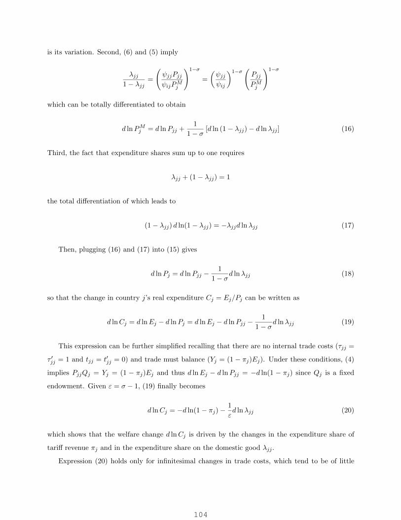
is its variation. Second, (6) and (5) imply

λjj1− λjj

=

(ψjjPjj

ψijPMj

)1−σ

=

(ψjjψij

)1−σ(Pjj

PMj

)1−σ

which can be totally differentiated to obtain

d lnPMj = d lnPjj +1

1− σ[d ln (1− λjj)− d lnλjj ] (16)

Third, the fact that expenditure shares sum up to one requires

λjj + (1− λjj) = 1

the total differentiation of which leads to

(1− λjj) d ln(1− λjj) = −λjjd lnλjj (17)

Then, plugging (16) and (17) into (15) gives

d lnPj = d lnPjj −1

1− σd lnλjj (18)

so that the change in country j’s real expenditure Cj = Ej/Pj can be written as

d lnCj = d lnEj − d lnPj = d lnEj − d lnPjj −1

1− σd lnλjj (19)

This expression can be further simplified recalling that there are no internal trade costs (τjj =

τ ′jj = 1 and tjj = t′jj = 0) and trade must balance (Yj = (1 − πj)Ej). Under these conditions, (4)

implies PjjQj = Yj = (1 − πj)Ej and thus d lnEj − d lnPjj = −d ln(1 − πj) since Qj is a fixed

endowment. Given ε = σ − 1, (19) finally becomes

d lnCj = −d ln(1− πj)−1

εd lnλjj (20)

which shows that the welfare change d lnCj is driven by the changes in the expenditure share of

tariff revenue πj and in the expenditure share on the domestic good λjj .

Expression (20) holds only for infinitesimal changes in trade costs, which tend to be of little

104

practical relevance. Nevertheless, it can be readily integrated to characterize the welfare effects of

discrete changes. This yields

Cj =1− πj1− π′j

(λjj

)− 1ε

(21)

where the share of tariff revenues in the actual and counterfactual equilibria are given by

πj =n∑i=1

tij1 + tij

λij and π′j =n∑i=1

t′ij1 + t′ij

λij λij

Hence, the welfare consequences of any arbitrary change in trade costs can indeed be computed

based only on few sufficient statistics: the trade elasticity and the change in the shares of expendi-

ture across goods.

However, knowing that only few sufficient statistics are needed to compute the welfare effects of

trade integration would be of little use unless we had a consistent way of identifying the values of

those statistics in the counterfactual scenario. This is clearly not much of a problem for the trade

elasticity ε, which, given utility (1), is constant by assumption. It may look more of a problem for

the counterfactual expenditure shares λ′ ={λ′ij

}. Luckily the structure of the model lends a hand.

Consider (6). As ψij is constant, taking log changes gives

d lnλij = d ln (Pij)1−σ − d ln (Pj)

1−σ

which, by (14), can be rewritten as

d lnλij = d ln (Pij)1−σ −

n∑i=0

λijd ln (Pij)1−σ (22)

As Qi is also constant, (4) implies

d ln (Pij)1−σ = d ln (φijYi)

1−σ

which allows one to restate (22) as

d lnλij = d ln (φijYi)1−σ −

n∑i=0

λijd ln (φijYi)1−σ

105

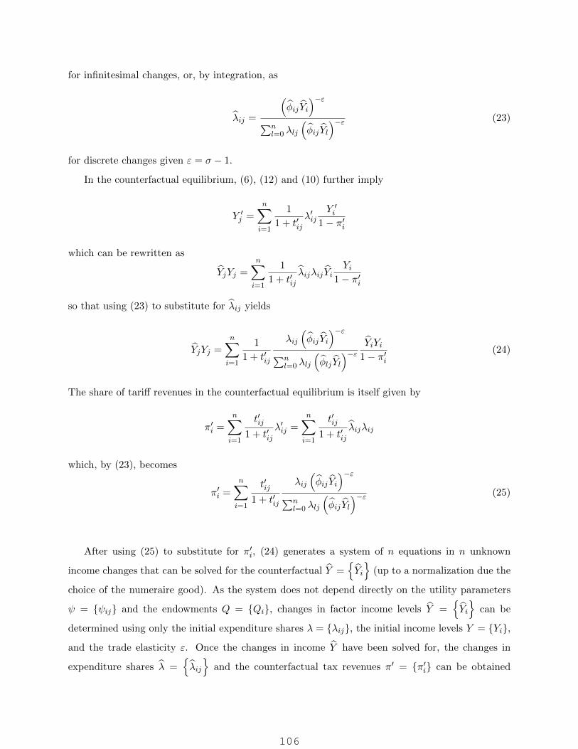
for infinitesimal changes, or, by integration, as

λij =

(φij Yi

)−ε∑n

l=0 λlj

(φij Yl

)−ε (23)

for discrete changes given ε = σ − 1.

In the counterfactual equilibrium, (6), (12) and (10) further imply

Y ′j =n∑i=1

1

1 + t′ijλ′ij

Y ′i1− π′i

which can be rewritten as

YjYj =

n∑i=1

1

1 + t′ijλijλij Yi

Yi1− π′i

so that using (23) to substitute for λij yields

YjYj =

n∑i=1

1

1 + t′ij

λij

(φij Yi

)−ε∑n

l=0 λlj

(φlj Yl

)−ε YiYi1− π′i

(24)

The share of tariff revenues in the counterfactual equilibrium is itself given by

π′i =

n∑i=1

t′ij1 + t′ij

λ′ij =

n∑i=1

t′ij1 + t′ij

λijλij

which, by (23), becomes

π′i =

n∑i=1

t′ij1 + t′ij

λij

(φij Yi

)−ε∑n

l=0 λlj

(φij Yl

)−ε (25)

After using (25) to substitute for π′i, (24) generates a system of n equations in n unknown

income changes that can be solved for the counterfactual Y ={Yi

}(up to a normalization due the

choice of the numeraire good). As the system does not depend directly on the utility parameters

ψ = {ψij} and the endowments Q = {Qi}, changes in factor income levels Y ={Yi

}can be

determined using only the initial expenditure shares λ = {λij}, the initial income levels Y = {Yi},

and the trade elasticity ε. Once the changes in income Y have been solved for, the changes in

expenditure shares λ ={λij

}and the counterfactual tax revenues π′ = {π′i} can be obtained

106

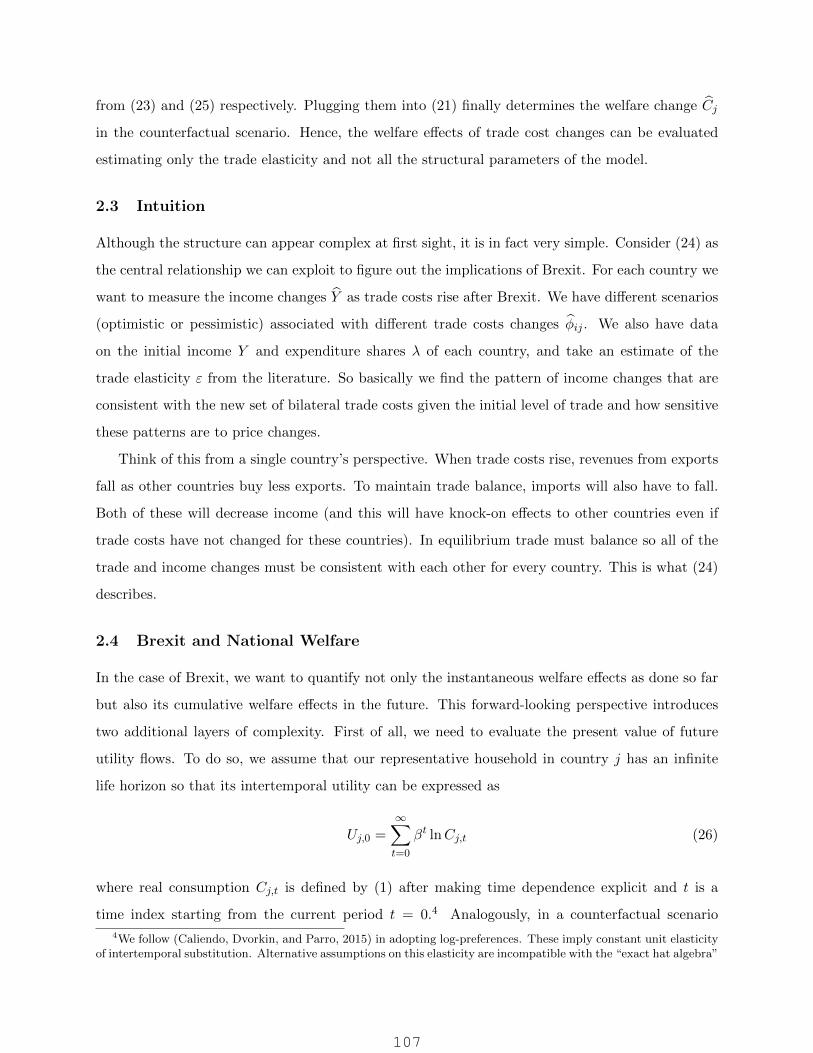
from (23) and (25) respectively. Plugging them into (21) finally determines the welfare change Cj

in the counterfactual scenario. Hence, the welfare effects of trade cost changes can be evaluated

estimating only the trade elasticity and not all the structural parameters of the model.

2.3 Intuition

Although the structure can appear complex at first sight, it is in fact very simple. Consider (24) as

the central relationship we can exploit to figure out the implications of Brexit. For each country we

want to measure the income changes Y as trade costs rise after Brexit. We have different scenarios

(optimistic or pessimistic) associated with different trade costs changes φij . We also have data

on the initial income Y and expenditure shares λ of each country, and take an estimate of the

trade elasticity ε from the literature. So basically we find the pattern of income changes that are

consistent with the new set of bilateral trade costs given the initial level of trade and how sensitive

these patterns are to price changes.

Think of this from a single country’s perspective. When trade costs rise, revenues from exports

fall as other countries buy less exports. To maintain trade balance, imports will also have to fall.

Both of these will decrease income (and this will have knock-on effects to other countries even if

trade costs have not changed for these countries). In equilibrium trade must balance so all of the

trade and income changes must be consistent with each other for every country. This is what (24)

describes.

2.4 Brexit and National Welfare

In the case of Brexit, we want to quantify not only the instantaneous welfare effects as done so far

but also its cumulative welfare effects in the future. This forward-looking perspective introduces

two additional layers of complexity. First of all, we need to evaluate the present value of future

utility flows. To do so, we assume that our representative household in country j has an infinite

life horizon so that its intertemporal utility can be expressed as

Uj,0 =

∞∑t=0

βt lnCj,t (26)

where real consumption Cj,t is defined by (1) after making time dependence explicit and t is a

time index starting from the current period t = 0.4 Analogously, in a counterfactual scenario

4We follow (Caliendo, Dvorkin, and Parro, 2015) in adopting log-preferences. These imply constant unit elasticityof intertemporal substitution. Alternative assumptions on this elasticity are incompatible with the “exact hat algebra”

107

intertemporal utility can be expressed as

U ′j,0 =∞∑t=0

βt lnC ′j,t.

The second layer of complexity comes from the fact that the future welfare effects of the UK

leaving the EU should be calculated relative not only to today’s welfare but also to the evolution

of future welfare if the UK stays in the EU. This implies that we have to compare the present value

of future utility between two counterfactuals: if the UK stays in the EU

U Inj,0 =∞∑t=0

βt lnCInj,t

and if the UK leaves

UOutj,0 =

∞∑t=0

βt lnCOutj,t .

Following (Sampson, 2016), we can then measure the welfare effects of Brexit by using the

consumption adjustment that makes the representative household indifferent between staying or

leaving the EU over its entire life span. This is measured by the value of the parameter δt such

that

U Inj,0(δj) =

∞∑t=0

βt(ln δj + lnCInj,t

)=

∞∑t=0

βt lnCOutj,t = UOutj,0

Solving this equation for ln δj gives the Brexit consumption equivalent change for country j

ln δBrexitj = (1− β)

∞∑t=0

βt(lnCOutj,t − lnCInj,t

)(27)

Accordingly, the welfare effects of Brexit can be quantified by evaluating (27). Note that, after

defining

ln δInj = (1− β)

∞∑t=0

βt ln CInj,t

and

ln δOutj = (1− β)∞∑t=0

βt ln COutj,t ,

we apply throughout in the wake of (Costinot and Rodriguez-Clare, 2013).

108

expression (27) can be equivalently rewritten as

ln δBrexitj = ln δOutj − ln δInj = (1− β)

∞∑t=0

βt(

ln COutj,t − ln CInj,t

)(28)

where CInj,t = CInj,t /Cj,t and COutj,t = COutj,t /Cj,t are the changes in real consumption in period t

relative to the status quo in period 0 if the UK stays and if the the UK leaves the EU respectively.

The idea is that, if the UK stays, it will enjoy any further fall in trade costs among EU members

relative to the status quo. The corresponding welfare effects are captured by the consumption

equivalent change δInj . On the other hand, if the UK leaves the EU, it will miss not only any

further fall in trade costs among EU members but might also face higher trade costs when trading

with EU members relative to the status quo. The corresponding welfare effects are captured by

δOutj .

2.5 Our Model

The Armington model has helped us to explain the basic logic of our approach, and in detail the

mechanics of its calibration and simulation procedure. It is, however, too stylized for our purposes.

Fortunately, (Costinot and Rodriguez-Clare, 2013) have shown that the gravity equation (7), which

is the basis for counterfactual analysis in the Armington model, holds under various assumptions

about technology and market structure. In what follows, we make the realistic choice of allowing

for multiple sectors and tradable intermediate inputs as well as the conservative choice of focusing

on the case of perfect competition as this has been shown to provide a lower bound to the welfare

effects of changes in trade costs.

Specifically, as in (Costinot and Rodriguez-Clare, 2013), we extend the model to multiple sectors,

indexed s = 1, ..., N , by assuming that the good consumed by the representative household in (26)

is a Cobb-Douglas basket of the goods supplied by the different sectors

Cj =∏S

s=1Cβj,sj,s

where, leaving time dependence t implicit for ease of notation, Cj,s is real consumption of the good

supplied by sector s and βj,s ∈ (0, 1) is its share of household expenditures with∑S

s=0 βj,s = 1.

By analogy with the single sector expression (21), the change in real consumption generated by a

109

counterfactual change in trade costs equals


∏S

s=1

(λjj,s

)−βj,sεs (29)

where the πj and π′j are again the shares of tariff revenue in country j’s expenditure in the current

and counterfactual scenarios respectively. Clearly, (29) boils down to (21) when we only have one

sector. To add also intermediates, we assume that each sector output is used not only in final

consumption but also, together with primary factors, as input for its own and any other sector’s

production. If we use αj,sk ∈ [0, 1] to denote the share of sector k’s output in sector s’s expenditure

on intermediate inputs, we get


∏S

s,k=1

(λjj,k

)−βj,saj,skεk (30)

where aj,sk is the elasticity of the price index in sector s with respect to changes in the price of

sector k. These price elasticities are given by the elements of the S × S Leontief inverse matrix

(Id− Aj)−1 where Aj is the matrix with typical element αj,sk. Expression (30) is what we use to

evaluate CInj,t and COutj,t for the quantification of the the welfare effects of Brexit through (28).

3 Empirical Analysis

In this section, we specify the time path of changes in the iceberg trade costs and tariffs if the UK

remains a member of the EU and if it does not under different scenarios. Then we quantify the

effects of such changes in tariff and/or trade costs on welfare and trade using the structural model

specified in previous section.

3.1 Data

We use the latest World Input-Output Database (WIOD) for year 2011.5. This database aggregates

the world into 40 countries and covers 35 sectors which we further aggregate into 35 regions and

31 sectors as in Costinot and Rodriguez-Clare (2013) We also collect information on the applied

most favoured nation (MFN) tariff by the EU from the World Trade Organization (WTO) website6,

which provides information on tariffs at the product level (HS classification) for all tradable goods.

5The data could be found at http://www.wiod.org/new_site/home.htm. For more details on how this databaseis constructed, see Dietzenbacher, Los, Stehrer, Timmer, and de Vries (2013).

6http://tariffdata.wto.org/

110

http://www.wiod.org/new_site/home.htm

http://tariffdata.wto.org/

We also use the United Nations (UN) Comtrade bilateral database at the product level. These two

datasets permit us to calculate an average MFN tariff at the WIOD sector level for UK imports

(exports), from (to) the EU by using import (export) value at the product level as weights. 7 The

resulting average MFN tariffs for imports and exports from/to the EU can be seen in Table A.3,

which summarizes the UK trade and MFN tariff information at the sector level. The table splits

the sectors between ’Goods’ and ’Services’.

The most intensively traded good in the UK/EU bilateral relationship is ’Transport Equipment’,

that includes auto-mobiles, amounting to 95.7 billion of US dollars in 2011. This sector also

possesses one of the highest average tariffs: 8.09% for imports from the EU and 7.22% for exports

to the EU. Note that most part of this trade is composed by imports (60.4 billion, or 63%). On the

other hand, the trade champion among services, the sector ’Renting of Machinery and Equip. and

Other Business Services’, is more intensively exported (USD 53 billions) than imported (USD 28

billion) by the UK. Financial services also are responsible for a significant trade share. Together,

the two former sectors are responsible for more than two thirds of the flows of services between the

UK and the EU. In general, we can see that the UK holds a deficit among goods and a surplus

among services, with reasonable variability within the two groups.

3.2 Counterfactuals

In this section we present counterfactual exercises associated with the UK leaving the EU. We

aim to quantify changes in welfare (real UK consumption) coming from three distinct sources: i)

immediate changes in goods tariffs, ii) immediate changes in non-tariff barriers, and iii) exclusion

from future market integration in the EU.

We consider two different scenarios. In the pessimistic case we assume that the UK is no longer

part of the single market and will trade with the EU under the regulations of the WTO. The UK

will apply the MFN tariffs seen in column (4) of Table A.3 on goods imported from the EU, while

the EU will apply the tariffs observed in column (7) on goods originating from the UK. This seems

reasonable just after withdrawal, but the hope is that the UK will eventually be able to negotiate a

better deal such as enjoyed by Norway and Iceland (in the European Economic Area) or Switzerland

(which has a series of bilateral deals). Hence, in our optimistic scenario we consider that tariffs on

goods continue to be zero between the UK and the EU.

Another important source of trade costs around the world is due to non-tariff barriers. Non-

7We aggregate HS 6-digit industries into 2-digit WIOD industries using a concordance between HS and ISIC Rev3.

111

tariff barriers are related to costs of shipment, differences in product regulations, legal barriers,

whether countries share a border, a common currency or language, search and other transaction

costs for both goods and services, etc (Anderson and van Wincoop, 2004; Head and Mayer, 2013).

Many authors point out that such costs are higher than formal tariffs (Anderson and van Wincoop,

2004; Novy, 2013; LooiKee, Nicita, and Olarreaga, 2009). In fact, most part of the negotiations

regarding the Transatlantic Trade and Investment Partnership between the EU and the USA aim

to diminish non-tariff barriers.

To incorporate non-tariff barriers we use information provided by Berden, Francois, Tamminen,

Thelle, and Wymenga (2009, 2013). The authors calculate detailed tariff equivalents of non-tariff

barriers between the USA and the EU, using econometric techniques and business surveys. They

also calculate the fraction of these non-tariff barriers that is reducible for each sector, i.e. the frac-

tion of the trade cost that could in principle be eliminated by policy action. We collect information

on sectors that can be easily matched to our classification shown in Table A.3. The sectors used,

their non-tariff costs (in tariff equivalent terms) and the share of the costs that can be reduced are

shown in Table A.1 in the Appendix.

As it is rather unlikely that the UK would face the same costs as the US in a case of withdrawal,

in our optimistic scenario we assume that the UK would face one quarter (1/4) of the reducible

cost faced by the USA, while in our pessimistic scenario we assume that they would face three

quarters (3/4). We calculate the weighted average of these cost shares, using total EU/UK trade

in each sector as weights and the subset of sectors shown in the Table A.1, which include several of

the relevant sectors in the EU/UK relationship. This calculation leads to an increase in non-tariff

costs of 2.01% and 6.04% in our optimistic and pessimistic scenarios, respectively. We then apply

such costs to all sectors in our economy.

We also consider that the intra-EU trade costs are falling over time (Ilzkovitz, Dierx, Kovacs,

and Sousa, 2007), and this rate is approximately 40% faster than in other OECD countries according

to Mejean and Schwellnus (2009), which uses panel data on French firms to study price convergence

in different markets between 1995 and 2004.8 We consider the scenario that 10 years from now

non-tariff barriers inside the EU would keep falling faster and the UK would not benefit from this

evolution. In our pessimistic scenario we assume that intra-EU non-tariff costs continue to fall 40%

faster than in the rest of the world. This may not necessarily be true since the OECD does not

include countries like China, which has seen a rapid decrease in trade costs with other countries.

8They find that the rate of price convergence is -0.412 for OECD countries -0.593 for EU countries.

112

Hence, in our optimistic scenario we assume that intra-EU barriers fall only 20% faster than in the

rest of the world.

To calculate this last counterfactual we need a measure of price differences across the EU. We

use a rough measure from Eaton and Kortum (2002) of 49%9, meaning that if the UK imported

(exported) all goods from (to) other European countries prices would be 49% higher. Naturally,

part of this price difference may not be reducible. We assume that the reducible proportion is 55%,

which is the same share of non-tariff barriers that are actionable in the EU-USA trade case. To

be conservative, in our pessimistic case we further assume that three quarters of the potentially

reducible share will actually diminish throughout the years, while in the optimistic case we assume

that such share is only one half. And to be even more conservative, we assume that the faster

market integration will peter out in 10 years after Brexit. And then, again using the estimates of

reducible price gaps from Mejean and Schwellnus (2009), we calculate the future falls of non-tariff

barriers within EU, which lead to a fall of 12.77% and 6.04% in our pessimistic and optimistic

scenarios respectively at year 10 after Brexit. 10

Armed with these numbers, we simulate the model by feeding in the sequence of shocks in trade

costs and tariffs for different scenarios of Brexit. The model then generates a sequences of changes

in real consumption. This allows us to compute the welfare change due to Brexit using equation

(28), assuming that the discount rate of future consumption is β = 0.96, which is a common value

in the macro literature.

Our results are shown in Table A.5. Panel A shows the result of the optimistic scenario. We

find that the welfare loss of the UK via the trade effect is 1.37%. How large are these numbers

when compared to the costs generated by the EU membership? HM Treasury (2013) estimates

that the net fiscal contribution of the UK to the EU is around 0.53% (or £ 8.6 billion) of the

UK GDP (2013). We assume that the UK would keep contributing 83% of the current per capita

contribution as Norway does in order to remain in the single market (House of Commons, 2013).

This leads to a fiscal saving of about 0.09%. Taking this benefit into account, the UK would still

lose a total of 1.28% in the case of an exit from the EU. We also calculate the implied loss per

household. In 2015 the UK had a population of about 65m with 27m households and a GDP of

£1.8 trillion. 1.28% of 1800/27 is £853 per household, which we round to £850 in the Table.

Panel B of Table A.5 shows the result of the pessimistic scenario. We see that the cost of a

9Table II, UK row average of the trade cost values.10Please refer Appendix B for the details of the computation.

113

withdrawal doubles. The UK loses 2.92% via trade due to higher tariff, non-tariff trade barriers

and exclusion from future further integration of the EU. Discounting the fiscal benefits still implies

a total welfare loss of 2.61%. This is equivalent to £1,700 per household.

We have shown the welfare losses suffered by the UK. We also estimate the effect of Brexit

on welfare for other countries again using equation (28). The results are shown in Figure C.1.

Two groups of countries have relatively larger welfare losses. First, countries for which UK is an

important trade partner, such as Ireland, Netherlands, Belgium, Denmark, Sweden, and Germany.

Figure C.2 shows the average expenditure share of intermediates sourcing from the UK across

sectors. These countries source relatively more intermediates from the UK, especially Ireland which

sources about 12% of intermediate inputs from the UK. A second group of countries that lose out

are those that do not trade much with the UK but exhibit a negative cross-sectoral correlation

between the expenditure share on intermediates sourcing from the UK and the trade elasticity.

Figure C.3 shows this correlation across countries. Countries such as Hungary, Czech Republic,

and Slovakia tend to trade more with the UK in sectors with relatively low trade elasticity. In

other words, if trade costs rise with the UK, they cannot easily substitute towards goods from

other countries. Thus they will have a relatively larger welfare loss as the prices they pay will rise

even if they trade relatively less with the UK.

Finally, countries outside EU tend to gain from Brexit, such as Russia, Turkey and China,

although the numbers are very close to zero. This is because of a trade diversion effect due to the

fact that the UK partially switches from trading with the EU to trading with non-EU countries

(which in turn benefit from more trade with UK). This can be illustrated by Table A.6. As we can

see, total British trade falls less than trade with the EU after Brexit.

4 Extensions and Robustness Checks

To check the robustness of our results to alternative assumptions, we first simulate the model for

two different scenarios. The results is shown in Panel A of Table A.8. The first scenario that

we simulate is the ”Swiss Alternative”. Switzerland is not in the EEA but has many bilateral

agreements with the EU, which give it some access to the single market. Like Norway, it has

to adopt all the regulations covering those parts of the single market it participates in and also

allows free movement of labour. It does, however, benefit from a lower fiscal transfer (about 40%

of the UK’s contribution on a per capita basis). On the other hand, it does not have free trade

114

in services with the EU, which would be a disadvantage for an economy like the UK, which has

a comparative advantage in services. We simulate the effects of Brexit using Switzerland as an

alternative optimistic scenario.

The result is very similar to the benchmark optimistic scenario - a loss of income of 1.28%.

Although the fiscal transfers are lower than for Norway (40% of 0.53% = 0.31% ) , these are more

than offset by higher costs of trade in services (a total welfare loss from lower trade of 1.6% vs.

1.37%).

Another scenario that we consider is what we call the Big Bang scenario. Under this scenario,

we assume that, if Brexit happens, the UK and the EU would impose MFN tariffs on each other

and the non-tariff trade barriers between the UK and the EU would rise to the reducible level

between the USA and the EU (+8.06%). Integration in the EU would continue to be 40% faster

than in the rest of world and 100% of the reducible price gaps could be reduced. However, the UK

would not benefit from such further integration. We assume that further integration would happen

in the year following Brexit, which implies that we are simulating the upper bound of welfare loss

for UK in our model. In this scenario we find that the UK welfare loss is about 3.5%.

Brexit campaigners have argued that the UK could neutralize the trade effect by unilaterally

liberalizing with all other countries. We check whether this is the case by removing all UK import

tariffs. We measure these import tariffs by constructing the sectoral MFN tariff as the weighted

average of HS 6-digit level UK imports from non-EU countries. The results are shown in Table A.2.

The overall weighted average UK MFN import tariff is around 3%. Feeding these tariffs into our

model for both the optimistic and pessimistic scenario, we find the effect of unilateral liberalization

is very limited as shown in Panel B of Table A.8. The welfare gain from removing the MFN import

tariff of the UK is just around 0.3%, far from neutralizing the adverse trade effect of Brexit. In the

optimistic case the income loss is 1% instead of 1.3% and in the pessimistic case the loss if 2.3%

instead of 2.6%. This is not surprising given that UK’s import tariffs are already very low.

In Panel C, we simulate the welfare loss of UK using alternative values of discount factor β

and fiscal benefits. So far, we have used a real interest rate of 4% which is standard in the macro

literature, but currently real interest rates are much lower than this, near zero in many cases. Using

a lower interest rate increases the costs of Brexit, because it gives larger weights to future losses

of income. For example, using a real interest rate of 1% leads to a welfare loss of 2.68% in the

optimistic case. Hence, given the current low interest rate, the results that we present in Table A.5

might actually understate the real loss.

115

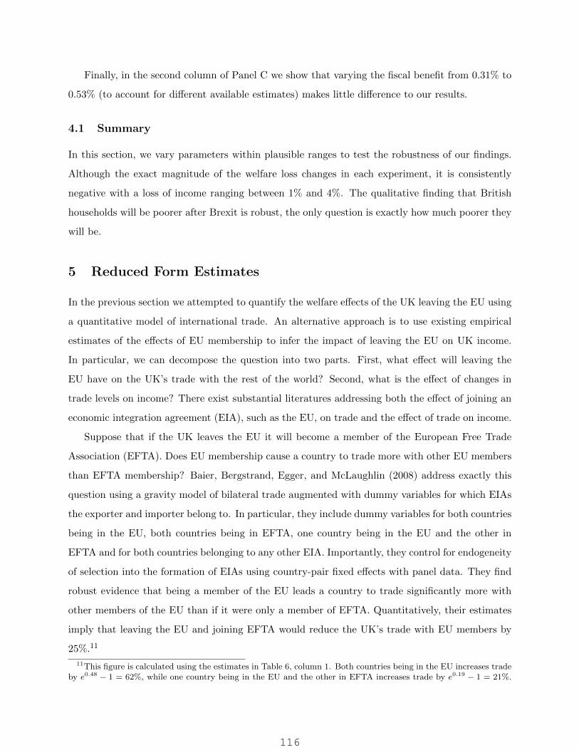
Finally, in the second column of Panel C we show that varying the fiscal benefit from 0.31% to

0.53% (to account for different available estimates) makes little difference to our results.

4.1 Summary

In this section, we vary parameters within plausible ranges to test the robustness of our findings.

Although the exact magnitude of the welfare loss changes in each experiment, it is consistently

negative with a loss of income ranging between 1% and 4%. The qualitative finding that British

households will be poorer after Brexit is robust, the only question is exactly how much poorer they

will be.

5 Reduced Form Estimates

In the previous section we attempted to quantify the welfare effects of the UK leaving the EU using

a quantitative model of international trade. An alternative approach is to use existing empirical

estimates of the effects of EU membership to infer the impact of leaving the EU on UK income.

In particular, we can decompose the question into two parts. First, what effect will leaving the

EU have on the UK’s trade with the rest of the world? Second, what is the effect of changes in

trade levels on income? There exist substantial literatures addressing both the effect of joining an

economic integration agreement (EIA), such as the EU, on trade and the effect of trade on income.

Suppose that if the UK leaves the EU it will become a member of the European Free Trade

Association (EFTA). Does EU membership cause a country to trade more with other EU members

than EFTA membership? Baier, Bergstrand, Egger, and McLaughlin (2008) address exactly this

question using a gravity model of bilateral trade augmented with dummy variables for which EIAs

the exporter and importer belong to. In particular, they include dummy variables for both countries

being in the EU, both countries being in EFTA, one country being in the EU and the other in

EFTA and for both countries belonging to any other EIA. Importantly, they control for endogeneity

of selection into the formation of EIAs using country-pair fixed effects with panel data. They find

robust evidence that being a member of the EU leads a country to trade significantly more with

other members of the EU than if it were only a member of EFTA. Quantitatively, their estimates

imply that leaving the EU and joining EFTA would reduce the UK’s trade with EU members by

25%.11

11This figure is calculated using the estimates in Table 6, column 1. Both countries being in the EU increases tradeby e0.48 − 1 = 62%, while one country being in the EU and the other in EFTA increases trade by e0.19 − 1 = 21%.

116

To predict the change in the UK’s overall trade we also need to know how leaving the EU

would affect the UK’s trade with non-EU members. Baier, Bergstrand, Egger, and McLaughlin

(2008) estimates suggest that whether a country is a member of the EU or EFTA does not have a

significant effect on its trade with EFTA members. However, their estimates do not address how

EU membership affects trade with countries outside of both the EU and EFTA. Structural gravity

models such as that developed by Egger, Larch, Staub, and Winkelmann (2011) can be used to

infer the general equilibrium effects of EIAs on trade between all country-pairs, but we are not

aware of any work that applies the structural gravity methodology to estimate the effects of EU

membership. Instead, we will rely on reduced form gravity model estimates of the trade diversion

effects of EIAs. Studies of trade diversion typically find little evidence that joining an EIA leads

to a reduction in trade with countries outside of the EIA. For example, Magee (2008) fails to find

robust evidence of significant trade diversion effects from EIAs. Therefore, we will assume that

leaving the EU will not affect the UK’s trade with the rest of the world.

To quantify the effect of trade on income we will use the estimates of Feyrer (2009). Using data

on the air and sea distances between countries, Feyrer (2009) uses changes in the cost of shipping

goods via air relative to sea as an instrument for trade in a regression of income on trade. Since

the instrument is time varying, Feyrer (2009) is able to improve upon the cross-section estimates of

Frankel and Romer (1999) by using country fixed effects to control for time invariant unobservable

that affect income levels. Feyrer (2009) concludes that the elasticity of income to trade is probably

between one-half and three-quarters. In other words, a 10% increase in trade increases income by

5% to 7.5%. The estimation strategy of Feyrer (2009) implies that his estimates capture both the

direct effect of higher trade on income and also other indirect effects of increased proximity between

countries such as variation in FDI and knowledge diffusion. Thus, the estimates we obtain in this

section should be interpreted as including some of the non-trade channels through which leaving

the EU will affect UK income in addition to the direct effect of changes in the UK’s trade.

Combining these numbers we can obtain a reduced form estimate of the effect of leaving the EU

and joining EFTA on UK income. Since 50.4% of the UK’s trade is with the EU, a 25% fall in trade

with EU members will reduce the UK’s overall trade by 12.6%. Combining this with the estimate in

Feyrer (2009) that the elasticity of income to trade is between one-half and three-quarters implies

Therefore, if a country leaves the EU and joins EFTA trade with EU members declines by (e0.19−e0.48)/e0.48 = 25%.To avoid confusion when interpreting the coefficient estimates in Baier, Bergstrand, Egger, and McLaughlin (2008)note that their EEA dummy variable is defined equal to one for a country pair when one country is in EFTA andthe other country is in the EU. Baier, Bergstrand, Egger, and McLaughlin (2008) do not estimate the effects of EEAmembership on trade, probably because the EEA was only established in 1994 and they use data from 1960-2000.

117

that leaving the EU and joining EFTA will reduce the UK’s income by between 6.3% and 9.5%.12

Interestingly, these calculations are similar to estimates of the historical benefits of EU membership

for the EU. For example, (Crafts, 2016) considers a range of papers that have sought to estimate

historically what the net benefit has been of EU membership. He concludes that the there was an

increase in UK GDP of around 8% to 10%.

The reduced form approach used in this section has two principal advantages over the structural

approach used earlier in the paper. First, it requires less detailed assumptions about what the

relationship between the UK and the EU would be following a UK exit. The structural estimates

required assumptions about both the future level of tariffs between the EU and the UK and the

extent to which the UK would share in future reductions in non-tariff barriers within the EU. By

contrast, the reduced form estimates are based on the simple and plausible assumption that if the

UK leaves the EU it will join EFTA. Second, while the quantitative trade model used above is

designed to capture only the static gains from trade, reduced form estimates of the effect of trade

on income should capture both static and dynamic effects.

The disadvantage of the reduced form approach is that it relies on the existence of unbiased

empirical estimates. While we have based our calculations on estimates obtained using best practice

empirical methodologies, sampling error and identification challenges inevitably mean that some

degree of uncertainty must be attached to the estimates. Overall, the calculations in this section

should be viewed as a robustness check on the plausibility of the predictions obtained from the

quantitative trade model. The reduced form estimates of the income effect of leaving the EU are

higher than those obtained from the quantitative trade model, but they reinforce the conclusion

that leaving the EU is likely to have a sizeable negative effect on UK welfare.

6 Conclusion

We have looked at different ways of estimating the change in UK living standards following a

decision to leave the EU. Using the Costinot and Rodriguez-Clare (2013) methodology, we generate

counterfactual scenarios and show that future losses in the UK due to this move can sum up to

1.28% of the GDP in real terms in our optimistic scenario, and to 2.61% in our pessimistic one.

12These estimates will understate the cost of leaving the EU if Baier, Bergstrand, Egger, and McLaughlin (2008)underestimate the decline in trade from leaving the EU and joining EFTA. Using the estimates in Table 5, column1 of Baier, Bergstrand, Egger, and McLaughlin (2008) implies the UK’s trade with EU members would decline by(e0.19 − e0.65)/e0.65 = 37% which implies a decline in UK income of between 9.3% and 13.9%. We chose to use theestimates in Table 6, column 1 to obtain a more conservative estimate of the costs of Brexit.

118

There are good reasons for thinking these under-estimate the real costs of Brexit as the evidence

looking at the historical impact of countries joining the EU has generated more trade and more

income than the static trade exercises we perform here would suggest. Using the reduced form

approach finds welfare losses of between 6.3% and 9.5%.

In any case, we should have in mind that these numbers are likely to be larger in reality, since

many other welfare improving channels associated with EU trade such as immigration, increases

in productivity, increases in R&D intensity, vertical production chains, to cite just a few, are not

considered in our analysis.

References

HM Treasury (2013): “European Union Finances 2013: statement on the 2013 EU Budget and

measures to counter fraud and financial mismanagement,” Discussion paper.

Albornoz, F., H. F. Calvo Pardo, G. Corcos, and E. Ornelas (2012): “Sequential export-

ing,” Journal of International Economics, 88(1), 17–31.

Anderson, J. E., and E. van Wincoop (2004): “Trade Costs,” Journal of Economic Literature,

42(3), 691–751.

Arkolakis, C., A. Costinot, and A. Rodriguez-Clare (2012): “New Trade Models, Same

Old Gains?,” American Economic Review, 102(1), 94–130.

Armington, P. S. (1969): “A Theory of Demand for Products Distinguished by Place of Produc-

tion (Une theorie de la demande de produits differencies d’apres leur origine)(Una teorıa de la de-

manda de productos distinguiendolos segun el lugar de produccion),” Staff Papers-International

Monetary Fund, pp. 159–178.

Baier, S. L., J. H. Bergstrand, P. Egger, and P. A. McLaughlin (2008): “Do Economic

Integration Agreements Actually Work? Issues in Understanding the Causes and Consequences

of the Growth of Regionalism,” The World Economy, 31(4), 461–497.

Baldwin, R. E., and A. J. Venables (1995): “Regional economic integration,” Handbook of

international economics, 3(3), 1597–644.

Berden, K., J. Francois, S. Tamminen, M. Thelle, and P. Wymenga (2009): “Non-Tariff

Measures in EU-US Trade and Investment: An Economic Analysis,” Final report, Ecorys.

119

(2013): “Non-Tariff Measures in EU-US Trade and Investment: An Economic Analysis,”

IIDE Discussion Papers 20090806, Institue for International and Development Economics.

Bloom, N., M. Draca, and J. Van Reenen (2015): “Trade induced technical change? The

impact of Chinese imports on Innovation, IT and Productivity,” Review of Economic Studies,

83(4), 87–117.

Caliendo, L., M. Dvorkin, and F. Parro (2015): “Trade and labor market dynamics,” NBER

Working Paper, 21149.

Caliendo, L., and F. Parro (2014): “Estimates of the Trade and Welfare Effects of NAFTA,”

The Review of Economic Studies, p. rdu035.

Costinot, A., and A. Rodriguez-Clare (2013): “Trade Theory with Numbers: Quantifying

the Consequences of Globalization,” CEPR Discussion Papers 9398, C.E.P.R. Discussion Papers.

Crafts, N. (2016): “The Growth effects of EU Membership for the UK: A Review of the Evi-

dence,” mimeo, University of Warwick.

di Giovanni, J., A. Levchenko, and F. Ortega (2015): “A Global View of Cross-Border

Migration,” CReAM Discussion Paper Series 1218, Centre for Research and Analysis of Migration

(CReAM), Department of Economics, University College London.

Dietzenbacher, E., B. Los, R. Stehrer, M. Timmer, and G. de Vries (2013): “The

Construction Of World Input–Output Tables In The Wiod Project,” Economic Systems Research,

25(1), 71–98.

Eaton, J., and S. Kortum (2002): “Technology, Geography, and Trade,” Econometrica, 70(5),

1741–1779.

Egger, P., M. Larch, K. E. Staub, and R. Winkelmann (2011): “The Trade Effects of

Endogenous Preferential Trade Agreements,” American Economic Journal: Economic Policy,

3(3), 113–43.

Feyrer, J. (2009): “Trade and Income – Exploiting Time Series in Geography,” NBER Working

Papers 14910, National Bureau of Economic Research, Inc.

Frankel, J. A., and D. H. Romer (1999): “Does Trade Cause Growth?,” American Economic

Review, 89(3), 379–399.

120

Harari, D., and G. Thompson (2013): “The economic impact of EU membership on the UK,”

Commons library standard note, Commons Library.

Head, K., and T. Mayer (2013): “Gravity Equations: Workhorse, Toolkit, and Cookbook,”

CEPR Discussion Papers 9322, C.E.P.R. Discussion Papers.

(2014): “Gravity Equations: Workhorse, Toolkit, and Cookbook,” Handbook of Interna-

tional Economics, 4.

House of Commons (2013): Leaving the EU, no. 13/42.

Ilzkovitz, F., A. Dierx, V. Kovacs, and N. Sousa (2007): “Steps towards a deeper economic

integration: the internal market in the 21st century,” European Economy - Economic Papers

271, Directorate General Economic and Monetary Affairs (DG ECFIN), European Commission.

Keller, W. (1999): “How Trade Patterns and Technology Flows Affect Productivity Growth,”

Working Paper 6990, National Bureau of Economic Research.

(2002): “Trade and the Transmission of Technology,” Journal of Economic Growth, 7(1),

5–24.

Krugman, P. (1980): “Scale Economies, Product Differentiation, and the Pattern of Trade,”

American Economic Review, 70(5), 950–59.

LooiKee, H., A. Nicita, and M. Olarreaga (2009): “Estimating Trade Restrictiveness In-

dices,” Economic Journal, 119(534), 172–199.

Magee, C. S. (2008): “New measures of trade creation and trade diversion,” Journal of Interna-

tional Economics, 75(2), 349–362.

Mejean, I., and C. Schwellnus (2009): “Price Convergence in the European Union: Within

Firms or Composition of Firms?,” Working Papers hal-00354190, HAL.

Melitz, M. J. (2003): “The Impact of Trade on Intra-Industry Reallocations and Aggregate

Industry Productivity,” Econometrica, 71(6), 1695–1725.

Melitz, M. J., and S. J. Redding (2014): “Missing Gains from Trade?,” CEP Discussion Papers

dp1254, Centre for Economic Performance, LSE.

121

Morris, N. (2013): “Former Chancellor Nigel Lawson calls for UK to leave European Union,”

Discussion paper, The Independent.

Novy, D. (2013): “Gravity Redux: Measuring International Trade Costs With Panel Data,”

Economic Inquiry, 51(1), 101–121.

Ottaviano, G. (2014): “European Integration and the Gains from Trade,” Routledge. Handbook

of the Economics of European Integration.

Piermartini, R., and R. Teh (2005): Demystifying modelling methods for trade policy, no. 10.

WTO Discussion Paper.

Sampson, T. (2016): “Dynamic Selection: An Idea Flows Theory of Entry, Trade and Growth,”

Quarterly Journal of Economics., 131(1), 315–80.

Simonovska, I., and M. E. Waugh (2014): “Trade models, trade elasticities, and the gains from

trade,” Discussion paper, National Bureau of Economic Research.

Springford, J., and S. Tilford (2014): “The Great British trade-off,” Discussion paper, Centre

for European Reform.

Wacziarg, R. (1998): “Measuring the dynamic gains from trade,” Policy Research Working Paper

Series 2001, The World Bank.

122

Appendix

A Tables

Table A.1: Sector and Non-tariff Barriers (NTB) used in the CounterfactualsNTB Cost EU+/USA Reducible share Weight

Sector (tariff equivalent) of NTB (total trade UK/EU)

Transport Equipment 22.1% 0.53 95723Chemicals and Chemical Products 23.9% 0.63 74797Post and Telecommunications 11.7% 0.70 8733Electrical and Optical Equipment 6.5% 0.41 61506Financial Intermediation 11.3% 0.49 50145Food, Beverages and Tobacco 5.8% 0.53 56463Construction 4.6% 0.38 3760Renting of Machinery & Equip. and Other Business Activities 14.9% 0.51 72628Services Nec (*) 4.4% 0.37 13561Basic Metals and Fabricated Metal 11.9% 0.62 44769Textiles and Textile Products; Leather, Leather and Footwear 19.2% 0.50 20178Wood and Products of Wood and Cork 11.3% 0.60 3413

Overall Weighted Average 14.7% 0.55 –

Source: WIOD and authors’ compilation of a subset of the sectors presented in Tables 3.3 and 4.2 of Berden,Francois, Tamminen, Thelle, and Wymenga (2009).Notes: The Table provides non-tariff costs (in tariff equivalent terms) of trade flows from the USA to the EU+(column 1). It also provides the share of costs that are potentially reducible (column 2). In our counterfactualswe assume either (i) that after Brexit the UK faces 1/4 of the reducible costs of the USA (optimistic scenario) or(ii) that after the exit the UK faces 3/4 of the reducible costs seen by the USA (pessimistic scenario). We thenuse total EU trade as weights (column 3) to compute a weighted average of these costs and apply to all sectors inall our counterfactuals. EU is defined as EU 28 minus the UK. EU+ includes the UK. Total trade in column (3)is the sum of all imports from the rest of the EU to the UK plus all exports from the UK to the EU (in millionsof US dollars). The overall weighted averages in the final row use column (3) numbers as weights.(*) Includes ’Repair of Household Goods’

123

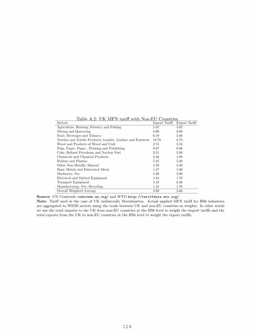
Table A.2: UK MFN tariff with Non-EU CountriesSectors Import Tariff Export Tariff

Agriculture, Hunting, Forestry and Fishing 1.07 4.02Mining and Quarrying 0.00 0.00Food, Beverages and Tobacco 6.19 2.08Textiles and Textile Products; Leather, Leather and Footwear 10.70 8.73Wood and Products of Wood and Cork 2.74 3.16Pulp, Paper, Paper , Printing and Publishing 0.07 0.06Coke, Refined Petroleum and Nuclear Fuel 2.51 3.36Chemicals and Chemical Products 2.46 1.89Rubber and Plastics 5.25 5.28Other Non-Metallic Mineral 4.79 3.49Basic Metals and Fabricated Metal 1.47 1.00Machinery, Nec 2.36 2.00Electrical and Optical Equipment 1.84 1.70Transport Equipment 5.43 6.26Manufacturing, Nec; Recycling 1.45 1.76

Overall Weighted Average 3.09 2.60

Source: UN Comtrade comtrade.un.org/ and WTO http://tariffdata.wto.org/.Note: Tariff used in the case of UK unilaterally liberalization. Actual applied MFN tariff for HS6 industriesare aggregated to WIOD sectors using the trade between UK and non-EU countries as weights. In other wordswe use the total imports to the UK from non-EU countries at the HS6 level to weight the import tariffs and thetotal exports from the UK to non-EU countries at the HS6 level to weight the export tariffs.

124

comtrade.un.org/

http://tariffdata.wto.org/

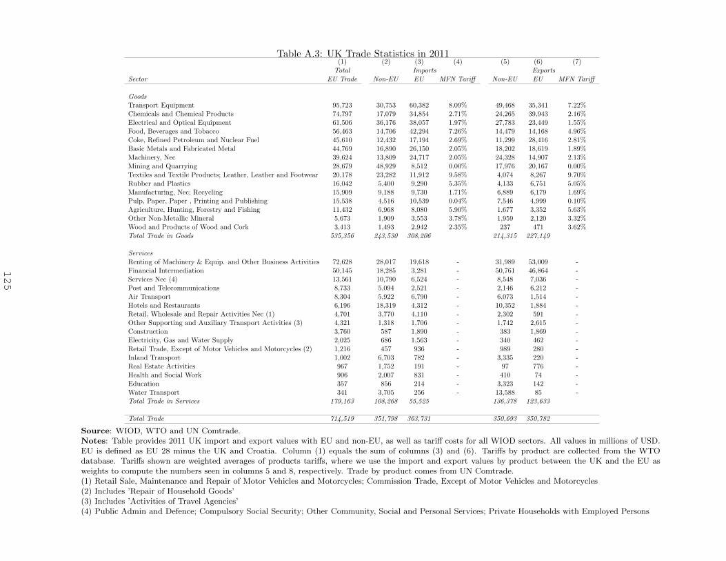
Table A.3: UK Trade Statistics in 2011(1) (2) (3) (4) (5) (6) (7)

Total Imports ExportsSector EU Trade Non-EU EU MFN Tariff Non-EU EU MFN Tariff

GoodsTransport Equipment 95,723 30,753 60,382 8.09% 49,468 35,341 7.22%Chemicals and Chemical Products 74,797 17,079 34,854 2.71% 24,265 39,943 2.16%Electrical and Optical Equipment 61,506 36,176 38,057 1.97% 27,783 23,449 1.55%Food, Beverages and Tobacco 56,463 14,706 42,294 7.26% 14,479 14,168 4.96%Coke, Refined Petroleum and Nuclear Fuel 45,610 12,432 17,194 2.69% 11,299 28,416 2.81%Basic Metals and Fabricated Metal 44,769 16,890 26,150 2.05% 18,202 18,619 1.89%Machinery, Nec 39,624 13,809 24,717 2.05% 24,328 14,907 2.13%Mining and Quarrying 28,679 48,929 8,512 0.00% 17,976 20,167 0.00%Textiles and Textile Products; Leather, Leather and Footwear 20,178 23,282 11,912 9.58% 4,074 8,267 9.70%Rubber and Plastics 16,042 5,400 9,290 5.35% 4,133 6,751 5.05%Manufacturing, Nec; Recycling 15,909 9,188 9,730 1.71% 6,889 6,179 1.69%Pulp, Paper, Paper , Printing and Publishing 15,538 4,516 10,539 0.04% 7,546 4,999 0.10%Agriculture, Hunting, Forestry and Fishing 11,432 6,968 8,080 5.90% 1,677 3,352 5.63%Other Non-Metallic Mineral 5,673 1,909 3,553 3.78% 1,959 2,120 3.32%Wood and Products of Wood and Cork 3,413 1,493 2,942 2.35% 237 471 3.62%Total Trade in Goods 535,356 243,530 308,206 214,315 227,149

ServicesRenting of Machinery & Equip. and Other Business Activities 72,628 28,017 19,618 - 31,989 53,009 -Financial Intermediation 50,145 18,285 3,281 - 50,761 46,864 -Services Nec (4) 13,561 10,790 6,524 - 8,548 7,036 -Post and Telecommunications 8,733 5,094 2,521 - 2,146 6,212 -Air Transport 8,304 5,922 6,790 - 6,073 1,514 -Hotels and Restaurants 6,196 18,319 4,312 - 10,352 1,884 -Retail, Wholesale and Repair Activities Nec (1) 4,701 3,770 4,110 - 2,302 591 -Other Supporting and Auxiliary Transport Activities (3) 4,321 1,318 1,706 - 1,742 2,615 -Construction 3,760 587 1,890 - 383 1,869 -Electricity, Gas and Water Supply 2,025 686 1,563 - 340 462 -Retail Trade, Except of Motor Vehicles and Motorcycles (2) 1,216 457 936 - 989 280 -Inland Transport 1,002 6,703 782 - 3,335 220 -Real Estate Activities 967 1,752 191 - 97 776 -Health and Social Work 906 2,007 831 - 410 74 -Education 357 856 214 - 3,323 142 -Water Transport 341 3,705 256 - 13,588 85 -Total Trade in Services 179,163 108,268 55,525 136,378 123,633

Total Trade 714,519 351,798 363,731 350,693 350,782

Source: WIOD, WTO and UN Comtrade.Notes: Table provides 2011 UK import and export values with EU and non-EU, as well as tariff costs for all WIOD sectors. All values in millions of USD.EU is defined as EU 28 minus the UK and Croatia. Column (1) equals the sum of columns (3) and (6). Tariffs by product are collected from the WTOdatabase. Tariffs shown are weighted averages of products tariffs, where we use the import and export values by product between the UK and the EU asweights to compute the numbers seen in columns 5 and 8, respectively. Trade by product comes from UN Comtrade.(1) Retail Sale, Maintenance and Repair of Motor Vehicles and Motorcycles; Commission Trade, Except of Motor Vehicles and Motorcycles(2) Includes ’Repair of Household Goods’(3) Includes ’Activities of Travel Agencies’(4) Public Admin and Defence; Compulsory Social Security; Other Community, Social and Personal Services; Private Households with Employed Persons

125

Table A.4: Trade Elasticity for each sectorWIOD31 sector code Sectors Trade Elasticity

1 Agriculture, Hunting, Forestry and Fishing 8.11

2 Mining and Quarrying 15.72

3 Food, Beverages and Tobacco 2.55

4 Textiles and Textile Products; Leather, Leather and Footwear 5.56

5 Wood and Products of Wood and Cork 10.83

6 Pulp, Paper, Paper , Printing and Publishing 9.07

7 Coke, Refined Petroleum and Nuclear Fuel 51.08

8 Chemicals and Chemical Products 4.75

9 Rubber and Plastics 1.66

10 Other Non-Metallic Mineral 2.76

11 Basic Metals and Fabricated Metal 7.99

12 Machinery, Nec 1.52

13 Electrical and Optical Equipment 10.6

14 Transport Equipment 0.37

15 Manufacturing, Nec; Recycling 5

16 Electricity, Gas and Water Supply 5

17 construction 5

18 Retail Sale of Fuel; Wholesale Trade, Commission Trade, including Motor Vehicles & Motorcycles 5

19 Retail Trade, Except of Motor Vehicles & Motorcycles; Repair of Household Goods 5

20 Hotels and Restaurants 5

21 Inland Transport 5

22 Water Transport 5

23 Air Transport 5

24 Other Supporting and Auxiliary Transport Activities; Activities of Travel Agencies 5

25 Post and Telecommunications 5

26 Financial Intermediation 5

27 Real Estate Activities 5

28 Renting of M&Eq and Other Business Activities 5

29 Education 5

30 Health and SocialWork 5

31 Public Admin, Defence, Social Security and othe public service 5

Source: The aggregation of the sectors are the same as (Costinot and Rodriguez-Clare, 2013). The trade elasticities for the tradable sectors are estimatedby Caliendo and Parro (2014). For the service sector, we follow (Costinot and Rodriguez-Clare, 2013) to set them as 5.

126

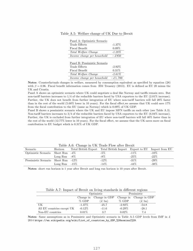
Table A.5: Welfare change of UK Due to Brexit

Panel A: Optimistic Scenario

Trade Effects -1.37%Fiscal Benefit 0.09%

Total Welfare Change -1.28%

Income change per household −£850

Panel B: Pessimistic ScenarioTrade Effects -2.92%Fiscal Benefit 0.31%

Total Welfare Change -2.61%

Income change per household −£1, 700

Notes: Counterfactuals changes in welfare, measured by consumption equivalent as specified by equation (28)with β = 0.96. Fiscal benefit information comes from HM Treasury (2013). EU is defined as EU 28 minus theUK and Croatia.Panel A shows an optimistic scenario where UK could negotiate a deal like Norway and tariffs remain zero. Butnon-tariff barriers increases to 1/4 of the reducible barriers faced by USA exporters to the EU (2.01% increase).Further, the UK does not benefit from further integration of EU where non-tariff barriers will fall 20% fasterthan in the rest of the world (5.68% lower in 10 years). For the fiscal effect,we assume that UK could save 17%from the fiscal contribution to the EU (same as Norway) which is 0.09% of UK GDP.Panel B shows a pessimistic scenario where the UK and EU impose MFN tariffs on each other (see Table A.3).Non-tariff barriers increases to 3/4 of the reducible barriers faced by USA exporters to the EU (6.04% increase).Further, the UK is excluded from further integration of EU where non-tariff barriers will fall 40% faster than inthe rest of the world (12.77% lower in 10 years). For the fiscal effect, we assume that the UK saves more on fiscalcontribution to EU budget which is 0.31% of UK GDP.

Table A.6: Change in UK Trade Flow after BrexitScenario Horizon Total British Export Total British Import Export to EU Import from EU

Optimistic Scenario Short Run -4% -5% -11% -10%Long Run -8% -8% -25% -22%

Pessimistic Scenario Short Run -12% -12% -31% -29%Long Run -15% -14% -44% -38%

Notes: short run horizon is 1 year after Brexit and long run horizon is 10 years after Brexit.

Table A.7: Impact of Brexit on living standards in different regionsOptimistic Pessimistic

Change in% GDP

Change in GDP(£ bn)

Change in% GDP

Change in GDP(£ bn)

UK -1.37% -25.7 -2.92% -54.8All EU countries except UK -0.12% -11.6 -0.29% -28.1Non-EU countries 0.01% 3.7 0.02% 7.4

Notes: Same assumptions as in Pessimistic and Optimistic scenario in Table A.5 GDP levels from IMF in £2014 https://en.wikipedia.org/wiki/List_of_countries_by_GDP_%28nominal%29.

127

https://en.wikipedia.org/wiki/List_of_countries_by_GDP_%28nominal%29

Table A.8: Robustness on welfare change of UK Due to Brexit

Panel A: Alternative scenariosScenarios A Swiss Alternative Big Bang

Trade effects −1.60% −4.02%Net UK fiscal contribution 0.31% 0.53%

Welfare Loss of UK −1.28% −3.49%

Panel B: Unilateral liberalisation of UKScenarios optimistic pessimistic

Trade effects −1.37% −2.92%Fiscal benefits 0.09% 0.31%Unilateral liberalisation 0.30% 0.32%

Welfare Loss of UK −0.98% −2.29%

Panel C: UK welfare loss under different parameters

Scenarios optimistic pessimistic

Discount factor: β = 0.99 −1.42% −2.68%Size of UK fiscal contribution to the EU −1.32% −2.39%

Notes: Panel A shows the results of the Swiss Alternative. Under such a scenario, the UK and EU still imposezero tariffs on goods flows. But unlike the optimistic scenario, the UK net fiscal contribution to EU would belower but the non-tariff barriers would be higher for services. To be precise, we assume the non-tariff tradebarriers for goods would be the same as the optimistic scenario and the non-tariff trade barriers for serviceswould be the same as the pessimistic scenario. Further, the UK saves 60% of the current fiscal transfer of 0.53%of GDP. In the Big Bang scenario, UK and EU trade is subjected to MFN tariff. Non-tariff barriers increaseby 8.01% between UK and EU but decrease between all other EU members by 15.88% following the year afterBrexit.Panel B shows the results of UK unilaterally liberalizing to all other countries. That is the UK imposes zerotariffs on all imported goods. The tariffs between UK and non-EU countries are shown in Table A.2.Panel C shows the welfare results for the optimistic and pessimistic scenario as we specified in Table A.5. Wefirst change the discount factor β from 0.96 to 0.99. In the second case, we alternate the size of the net fiscaltransfer from UK to the EU from 0.53% to 0.31% of GDP for the optimistic scenario and from 0.31% to 0.53%of GDP for the pessimistic scenario.

128

Table A.9: Aggregation of RegionsWIOD Country WIOD CODE Aggregation

Australia AUS AUSAustria AUT AUTBelgium BEL BELBrazil BRA BRACanada CAN CANChina CHN CHNCzech Republic CZE CZEGermany DEU DEUDenmark DNK DNKSpain ESP ESPFinland FIN FINFrance FRA FRAUnited Kingdom GBR GBRGreece GRC GRCHungary HUN HUNIndia IDN IDNIndonesia IND INDIreland IRL IRLItaly ITA ITAJapan JPN JPNKorea KOR KORMexico MEX MEXNetherlands NLD NLDPoland POL POLPortugal PRT PRTRomania ROM ROMRussia RUS RUSSlovakia SVK SVKSlovenia SVN SVNSweden SWE SWETurkey TUR TURTaiwan TWN TWNUnited States USA USA

Bulgaria BGRCyprus CYPEstonia ESTLatvia LVA RoEULithuania LTULuximburg LUXMalta MLT

Rest of World ROW ROW

Notes: We aggregate the WIOD regions shown in column(1) to those shown in column(3).

129

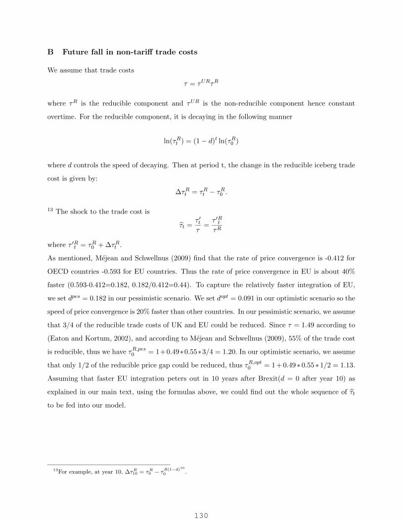
B Future fall in non-tariff trade costs

We assume that trade costs

τ = τURτR

where τR is the reducible component and τUR is the non-reducible component hence constant

overtime. For the reducible component, it is decaying in the following manner

ln(τRt ) = (1− d)t ln(τR0 )

where d controls the speed of decaying. Then at period t, the change in the reducible iceberg trade

cost is given by:

∆τRt = τRt − τR0 .

13 The shock to the trade cost is

τt =τ ′tτ

=τ ′RtτR

where τ ′Rt = τR0 + ∆τRt .

As mentioned, Mejean and Schwellnus (2009) find that the rate of price convergence is -0.412 for

OECD countries -0.593 for EU countries. Thus the rate of price convergence in EU is about 40%

faster (0.593-0.412=0.182, 0.182/0.412=0.44). To capture the relatively faster integration of EU,

we set dpes = 0.182 in our pessimistic scenario. We set dopt = 0.091 in our optimistic scenario so the

speed of price convergence is 20% faster than other countries. In our pessimistic scenario, we assume

that 3/4 of the reducible trade costs of UK and EU could be reduced. Since τ = 1.49 according to

(Eaton and Kortum, 2002), and according to Mejean and Schwellnus (2009), 55% of the trade cost

is reducible, thus we have τR,pes0 = 1+0.49∗0.55∗3/4 = 1.20. In our optimistic scenario, we assume

that only 1/2 of the reducible price gap could be reduced, thus τR,opt0 = 1 + 0.49 ∗ 0.55 ∗ 1/2 = 1.13.

Assuming that faster EU integration peters out in 10 years after Brexit(d = 0 after year 10) as

explained in our main text, using the formulas above, we could find out the whole sequence of τt

to be fed into our model.

13For example, at year 10, ∆τR10 = τR0 − τR(1−d)100 .

130

C Graphs

Figure C.1: Welfare loss across countries

Notes: same assumptions as in notes to Table A.5 except net fiscal savings not included. The listof countries could be found in A.9

131

Figure C.2: Average share of intermediates sourcing from UK across sectors

Notes: The share is the simple average of input value share sourcing from the UK across 31WIOD sectors.

Figure C.3: Correlation between expenditure share on UK goods and trade elasticity

Notes: The figure plots the expenditure share on UK goods with the trade elasticity for eachcountry.

132

#CE

PB

RE

XIT

PA

PE

RBR

EXIT

TECHNICAL PAPER‘The impact of Brexit on foreign

investment in the UK’

Technical Appendix to ‘The Impact of Brexit on

Foreign Investment in the UK’

Gravitating Towards Europe:

An Econometric Analysis of the

FDI Effects of EU Membership

Randolph Bruno

(UCL and IZA-Bonn)

[email protected]

Nauro Campos

(Brunel University London, ETH-Zurich and IZA-Bonn)

[email protected]

Saul Estrin

(LSE, CEP and IZA-Bonn)

[email protected]

Meng Tian

(Peking University)

[email protected]

How much additional foreign direct investment (FDI) does a country receive as a

consequence of being a member of the European Union (EU)? The objective of this

paper is to offer novel estimates of the effect of EU membership on FDI inflows

using bilateral FDI data from 34 OECD countries 1985-2013. We find that EU

membership robustly increases FDI inflows by 14% to 38% depending on the choice

of econometric techniques. Should the UK leave the EU, we predict about a 22%

fall in FDI inflows. Our results are robust to the use of more sophisticated

econometric estimators. In light of the recent debates on Brexit, we also try to

understand the reasons for foreign investors choosing the UK vis-à-vis other

European countries, emphasising the potential effects of European integration on

FDI inflows to the UK.

* We would like to thank, without implicating, Swati Dhingra, John Van Reenen and

seminar participants at NIESR and LSE for valuable comments on previous versions.

134

1 Introduction

The gravity model has been a staple of international economics. It explains bilateral cross-

border flows (trade, migration, investment, etc.) based on the relative size and distance between

countries or regions (see Head and Mayer, 2014, for an authoritative review). A country’s

economic size is expected to have a positive effect on bilateral flows while distance is expected

to have a negative effect (distance is often taken to reflect a whole range of trade costs including

language, bureaucracy, culture, etc.).

The last two decades have witnessed enormous progress in this area. Among many

influential pieces, Anderson and van Wincoop (2003) and Santos Silva and Tenreyro (2006)

are the crucial ones for our present purposes. This new Structural Gravity approach (Fally,

2015) provides needed theoretical underpinnings as well as strong support for the econometric

estimation of gravity models.

This paper offers novel estimates of the effect of membership of the European Union (EU)

on inflows of foreign direct investment (FDI). As such, it is motivated by two concerns. The

first motivation is that although the benefits of FDI are well established in the economic

literature,1 there is a dearth of analysis of its impact within the European integration experience.

Inward FDI is a major contributor to the diffusion of managerial best practices (Bloom et al,

2012). It increases competition and shores up technological innovation; and it is believed to do

so in a more resilient and sustainable fashion than other international capital flows. Despite the

obvious importance of the subject, the literature focusing on potential reasons for foreign

investors to choose the UK vis-à-vis say Germany, Poland or Switzerland remains scarce. We

try to address this gap. European integration may have played a significant role and we need a

good understanding of these potential effects.

The second motivation refers to the potential value of an indirect comparison between the

trade effects of the EU and the FDI effects of currency unions like the euro. For example, Glick

and Rose (2016) find that their earlier estimates (Glick and Rose, 2002) on the impact of

currency unions were statistically fragile when subject to a wide range of modern econometric

techniques. Most of these new techniques were developed and used in the estimation of gravity

models after they published their original paper.

We therefore ask whether the use of modern econometric techniques eliminates the effects

of the EU on FDI. We find that it does not. EU membership significantly increases FDI inflows

1 For example, see Alfaro et al (2004) on international macro data or Haskel et al (2007) on UK micro-data.

135

by around 28% depending on the precise choice of econometric technique. We show that this

finding is consistent with alternative methodologies that look specifically at the UK experience

of FDI compared to other countries (Campos and Coricelli, 2015).

This Appendix is structured as follows. Section 2 introduces the gravity model, Section 3

the synthetic cohort approach and Section 4 the data. Section 5 presents the main new empirical

findings of the positive effects of being in the EU from a gravity model of bilateral FDI flows.

Section 6 concludes.

2 The gravity model

Gravity has gravitas. The original gravity study was authored by Jan Tinbergen, the first winner

of the Nobel Prize in Economics. These original estimations used pooled OLS methods without

time or country fixed effects. The inclusion of fixed effects has (justifiably) become a standard

estimation feature, usually by adding ‘dyadic effects’ (that is, a dummy variable for each pair

of countries involved in a bilateral flow). These control for any time-invariant characteristic

common to every pair of trading partners. A number of important issues fall into this category,

particularly distance between countries and whether they share a common culture, language or

border. The subsequent step in the evolution of gravity modelling was the use of time-varying

country and dyadic fixed effects. The current stage in the evolution of modelling gravity is the

Poisson estimator (Santos Silva and Tenreyro, 2006).

Baldwin (2006) and Baldwin and Taglioni (2007) provide important insights for the

application of the gravity model in the empirical analysis. They derive the basic gravity

equation for trade that we use for FDI:

ln(Bilateral Inflow of FDIo,d,t) = α0 +α1lnXo,t + α2lnXd,t + α3Zo,d,t+ �o,d + uo,d,t

where ln(.) stands for a natural logarithm and the Xo,t is a vector of characteristics of the origin

country, o, in year t. This will include measures of the size (GDP) and wealth (GDP per capita)

of the country. Similarly Xd,t is a vector of destination nations’ characteristics. The Zo,d,t is a

vector of characteristics specific to a country pair and will include things like geographical

distance (a proxy for trade costs) and cultural distance (colonial history, common language,

etc.). Being a member of the EU will be one of the time-varying observable characteristics of

a country that enter the Xo,t and Xd,t. vector. Many FDI-relevant characteristics will be hard to

control for with observables, which is why including a dyadic fixed effect (�o,d) is so important

(a dummy variable for each pair of countries – around 630 fixed effects). Since culture and

136

geography do not change much over time, the fixed effects will control for them, so the

coefficients of interest are identified from the impact of changes in trading relationships (and

other economic variables) over time on the change in FDI flows over time. The uo,d,t is an error

term that includes a full set of time dummies to control for global macroeconomic shocks. The

standard errors are clustered by dyadic pair to allow for serial correlation of the errors.

3 FDI in the UK after 1970: a synthetic cohort approach

The UK is one of the main FDI recipients in Europe. Net FDI inflows to the UK were small in

absolute terms until the mid-1990s, but afterwards they exhibit two periods of rapid expansion,

one in the second half of the 1990s and the other before the financial crisis. The 2008 financial

crisis generated a substantial ‘sudden stop’ in FDI inflows (see Figure 1).

Campos and Coricelli (2015) use these data to provide some estimates of the effects of the

Single Market on UK FDI net inflows. In Figure 1, the dashed red line shows their ‘synthetic

counterfactual’ estimates, showing what would have been FDI net inflows after 1986 if the UK

had decided not to join the Single Market.2 The results suggest that the Single Market played a

key role in mobilising FDI to and from the UK. Interestingly, they show that the bulk of these

benefits (in terms of additional UK FDI, had the UK chosen to opt out instead) occurred post-

euro, between the dot-com bubble and the financial crisis. In other words, these results suggest

that for the whole period of 1986 to 2014, the UK would have received on average about 25%

to 30% less FDI had it not been in the EU, but that this average conceals large variations over

time that deserve further study.

2 These results use the Synthetic Control Method pioneered by Abadie and Gardeazabal (2003) and originally

reported in Campos and Coricelli (2015). They are based on a simple model focusing on market size, per capita

GDP and trade openness as key determinants of location choice. The following estimated weights were obtained:

the United States (20%), Canada (44%) and New Zealand (36%). Data source is World Bank’s World

Development Indicators.

137

Figure 1:

What would UK FDI net inflows be if the UK had not been in the EU Single Market?

Source: Campos and Coricelli (2015).

Notes: FDI is measured in nominal US$. The actual FDI flows for the UK (solid black line) are compared to a

counterfactual (dashed line) of a ‘synthetic UK’ made up of a weighted basket of three other countries (the United

States, Canada and New Zealand). Vertical line is when the EU Single Market Programme set up.

4 Data and modelling strategy

To estimate the impact of EU membership on FDI, we collected the most recently available

data on bilateral FDI flows, GDP and GDP per capita (sender and target), bilateral distance and

the shares of manufacturing output, exports and imports in total GDP. Table 1 reports

definitions and sources, while Table 2 reports basic descriptive statistics.

Our data set covers 34 OECD countries between 1985 and 2013.3 Our data represent more

than 70% of global FDI inflows and, because the countries are all OECD members, they are

collected in a homogenous manner and are of relatively high quality. The main disadvantage

of our data is the exclusion of most developing countries including China and India. Notice

that a by-product of this drawback is that we are limited in the currency unions we can study

(for example, vis-à-vis Glick and Rose, 2016).

3 The maximum theoretical number of observations is 34*33*29=32,538. For many countries, especially before

the 1980s, bilateral FDI flows are in fact zero. The missing values for FDI in the data reflect these zeros (and a

few near zero). Missing observations are assigned zeros (which explains the different number of observations in

Tables 2 and 3). We used the Heckman selection model to try to deal with whether we should treat zero FDI in a

special way.

138

Table 1: List of variables

Definition Unit Source

Bilateral FDI flow Inward FDI flows (sender

to target)

USD, Millions OECD database

Bilateral FDI stocks Inward FDI Stocks (sender

to target)

USD, Millions OECD database

GDP (sender) Total GDP of FDI sender USD, millions World Bank

GDP (target) Total GDP of FDI target USD, millions World Bank

GDP per capita (sender) GDP per capita of FDI

sender

USD, PPP World Bank

GDP per capita (target) GDP per capita of FDI

target

USD, PPP World Bank

EU member (sender) Sender country is EU

member

0,1 EU website

EU member (target) Target country is EU

member

0,1 EU website

Manufacturing share (target) Share of manufacturing

output as percentage of

total GDP

% World Bank

Export share (target) Share of export as

percentage of total GDP

% World Bank

Import share (target) Share of import as

percentage of total GDP

% World Bank

Notes: ‘Target’ indicates the country that is the recipient of the FDI and ‘sender’ indicates the country that is the

sender of the FDI.

Table 2: Summary statistics

Obs. Mean CV

(SD/mean)

p25 p50 p75

Bilateral FDI inward

flow

19,241 680 6.23 0 6.5 190.2

Bilateral FDI inward

stock

16,880 7371 3.53 0 289.6 3154.8

GDP (sender) 19,834 1,056,215 2.04 150,218.9 310,006.2 1,121,872.0

GDP (target) 19,776 1,088,197 1.97 169,867.0 368,753.4 1,162,375.0

GDP per capita (sender) 19,682 27,324 0.47 18,224.8 25,859.9 344,41.4

GDP per capita (target) 19,776 26,764 0.49 17,298.7 25,221.5 340,82.7

EU member (sender) 20,268 1 0.97 0.0 1.0 1.0

EU member (target) 19,788 1 0.85 0.0 1.0 1.0

Manufacturing share of

GDP(target)

16,283 18 0.29 13.8 17.8 21.6

Export/GDP (target) 19,776 40 0.66 24.1 31.6 49.0

Import/GDP (target) 19,776 38 0.58 25.1 31.4 44.7

Notes: ‘Target’ indicates the country that is the recipient of the FDI and ‘sender’ indicates the country that is the

sender of the FDI. SD = Standard Deviation; p25=25th percentile; p50=median and p75=75th percentile.

139

Our modelling strategy follows the standard structural gravity approach. For example, a

similar specification is used by Baier and Bergstrand (2007, their equations (9) and (10)). First,

we estimate a baseline model using the natural logarithm of bilateral FDI flows; second, we

estimate a Poisson model; and finally, we estimate a Heckman model that takes into account

the zero flows bilateral trade and as such has a larger number of observations. In all cases, we

control for dyadic fixed effects and time dummies.

Dyadic fixed effects and time dummies matter. The inclusion of bilateral fixed effects

helps to minimise the effects of the exclusion of many of the usual suspects in explaining FDI

flows. They control for country pair unobserved heterogeneity and implicitly for factors such

as cultural distance, bilateral regulatory agreements, etc. The usual concern regarding ‘omitted

variable bias’ is mitigated in this way in these types of models. Year fixed effects are also

important. They reflect the macro phenomena that are common across all country-pairs.

Finally, we also address a selection problem. Suppose that the OLS and Poisson regression

are biased by the inclusion of ‘positive only’ data of bilateral FDI flows. 41% of the

observations are zero and the OLS model deals with this by giving a value of $1 of FDI to the

missing value so we can take logarithms. But this is rather arbitrary and the fact that there are

no bilateral trade flows between two countries may be telling us more about the sunk costs of

doing business between the pair of countries.

We try to address this issue via a Heckman selection model in which we first estimate a

selection equation (column (4)). The likelihood of non-zero flows is modelled as a function of

manufacturing, exports and import shares as well as the per capita GDP of the destination

country. The selection equation generates some interesting lessons: a higher likelihood of

positive FDI flows is related to lower per capita GDP in the destination country (FDI goes to

countries where the return to capital is higher), higher industry shares (better integration in the

value chain), lower export shares (substitution effect) and higher import shares of the target.4

4 The lambda term is significant and negative, suggesting that the error terms in the selection and primary

equations are negatively correlated and the selection equation is needed.

140

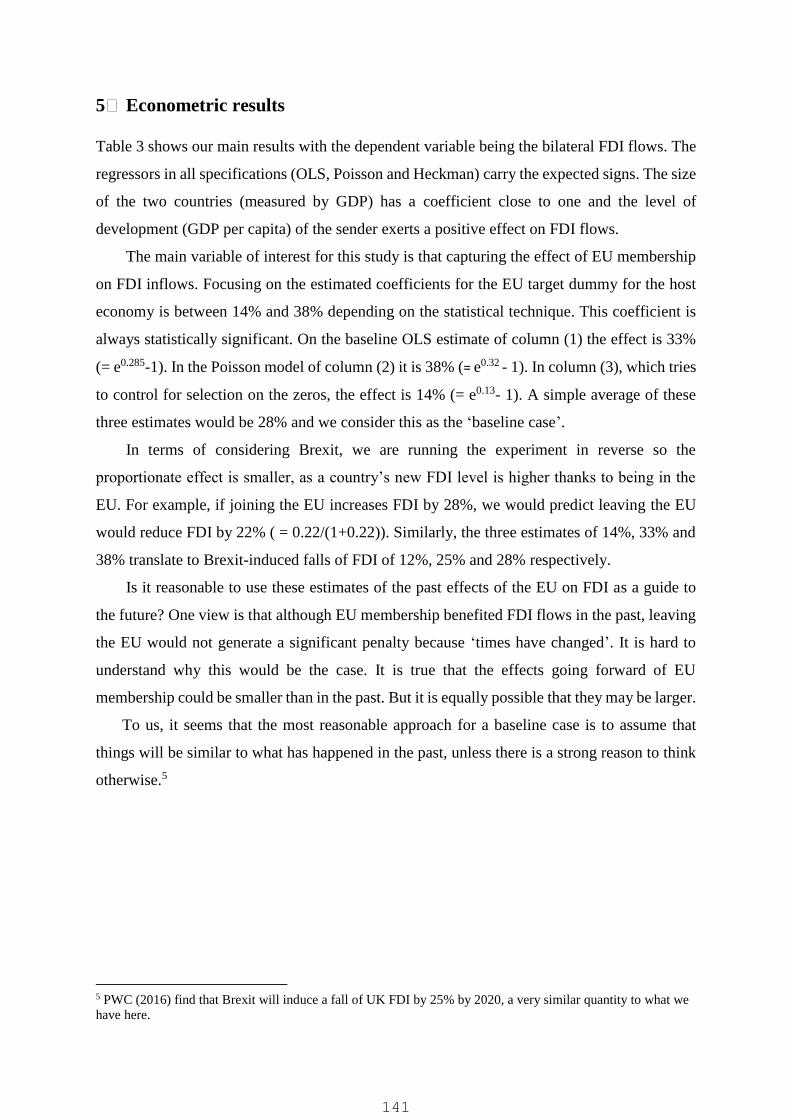
5 Econometric results

Table 3 shows our main results with the dependent variable being the bilateral FDI flows. The

regressors in all specifications (OLS, Poisson and Heckman) carry the expected signs. The size

of the two countries (measured by GDP) has a coefficient close to one and the level of

development (GDP per capita) of the sender exerts a positive effect on FDI flows.

The main variable of interest for this study is that capturing the effect of EU membership

on FDI inflows. Focusing on the estimated coefficients for the EU target dummy for the host

economy is between 14% and 38% depending on the statistical technique. This coefficient is

always statistically significant. On the baseline OLS estimate of column (1) the effect is 33%

(= e0.285-1). In the Poisson model of column (2) it is 38% (= e0.32 - 1). In column (3), which tries

to control for selection on the zeros, the effect is 14% (= e0.13- 1). A simple average of these

three estimates would be 28% and we consider this as the ‘baseline case’.

In terms of considering Brexit, we are running the experiment in reverse so the

proportionate effect is smaller, as a country’s new FDI level is higher thanks to being in the

EU. For example, if joining the EU increases FDI by 28%, we would predict leaving the EU

would reduce FDI by 22% ( = 0.22/(1+0.22)). Similarly, the three estimates of 14%, 33% and

38% translate to Brexit-induced falls of FDI of 12%, 25% and 28% respectively.

Is it reasonable to use these estimates of the past effects of the EU on FDI as a guide to

the future? One view is that although EU membership benefited FDI flows in the past, leaving

the EU would not generate a significant penalty because ‘times have changed’. It is hard to

understand why this would be the case. It is true that the effects going forward of EU

membership could be smaller than in the past. But it is equally possible that they may be larger.

To us, it seems that the most reasonable approach for a baseline case is to assume that

things will be similar to what has happened in the past, unless there is a strong reason to think

otherwise.5

5 PWC (2016) find that Brexit will induce a fall of UK FDI by 25% by 2020, a very similar quantity to what we

have here.

141

Table 3: Panel estimates of the effects of EU membership on FDI inflows

Dependent variable:

Dependent Variable:

(1)

Ln(1 + FDI)

(2)

FDI

(3)

Ln(FDI)

(4)

Dummy

1(FDI>0)

EU member (target) 0.285*** 0.320* 0.132***

(0.077) (0.163) (0.050)

EU member (sender) -0.010 0.828*** 0.199***

(0.079) (0.191) (0.050)

Ln(GDP, target) 0.473*** 3.799*** 0.686***

(0.056) (1.432) (0.226)

Ln(GDP, sender) 0.500*** 3.903*** 0.766***

(0.154) (1.462) (0.226)

Ln(GDP per capita, target) 0.180 -1.489 -0.010 0.230***

(0.158) (1.513) (0.255) (0.017)

Ln(GDP per capita, sender) 1.450*** -1.125 1.655***

(0.154) (1.623) (0.254)

Manufacturing value added/GDP 0.005***

(target) (0.002)

Exports/GDP -0.013***

(target) (0.001)

Imports/GDP 0.011***

(target) (0.002)

Mills’ Ratio 1.043***

(0.164)

Observations 33,524 33,147 33,524 33,524

Notes: *** indicates significance at the 1% level, ** at the 5% level and * at the 10% level. Coefficients with

standard errors (clustered by 630 bilateral country pair in first two columns) in brackets. All regressions include

fixed effects for years and dyadic pair. Column (1) is estimated by OLS. Column (2) is estimated by Poisson PML.

Columns (3) and (4) are a two-part Heckman selection equation. The dependent variable in column (4) is a dummy

equal to 1 if there are any FDI inflows and zero otherwise. The Mills’ ratio is constructed from this column and

included in column (3). The 34 OECD countries included are Austria, Australia, Belgium, Canada, Chile, Czech

Republic, Denmark, Estonia, Finland, France, Germany, Greece, Hungary, Iceland, Ireland, Israel, Italy, Japan,

Korea, Luxembourg, Mexico, Netherlands, Norway, New Zealand, Poland, Portugal, Slovakia, Slovenia, Spain,

Sweden, Switzerland, Turkey, UK and the US. ‘Target’ indicates the country which is the recipient of the FDI

and ‘sender’ indicates the country is the sender of the FDI.

142

We have subjected our estimates to a wide range of robustness checks. First, we are

implicitly treating the counterfactual to EU membership as simply being a standard member of

the World Trade Organization (WTO), whereas we may believe being in the European Free

Trade Association (EFTA) or the European Economic Area (EEA) is a more optimistic

alternative for the UK after leaving the EU – so-called ‘Brexit’ (Dhingra et al, 2016). If we add

two dummy variables for being an EFTA sender or receiver to column (1) both coefficients are

statistically insignificant and the EU recipient dummy remains positive and significant (0.211

with a standard error of 0.100). This suggests that it is being in the EU that matters. Further,

the point estimate on being an EFTA recipient is actually negative (-0.206 with a standard error

of 0.144). This implies that there may be some trade diversion from EFTA members like

Switzerland to EU members (for example, because Switzerland is not in the Single Market for

financial services).

Second, we have focused on modelling flows, but an alternative would be to use FDI

stocks. This gives qualitatively similar results. The EU recipient dummy always attracts a

positive coefficient in the three alternative estimators in the equivalent columns to Table 3.

Third, we examine some of the dynamic impacts of EU membership. We find that the big

effects came quite quickly following membership rather than taking a long time to feed

through.

How do these results compare with other estimates in the literature? As noted in Section

2, the synthetic cohort approach generates effects of 25% to 30% for the UK, which are very

much in the same ballpark.

Straathof et al (2008) also use a gravity model to look at bilateral FDI stocks. One of their

specifications uses dyadic fixed effects but a somewhat different set of controls and on earlier

data (1981-2005). They find that if a country is in the EU, it enjoys a 28% increase in its inward

FDI stocks from other EU countries and a 14% increase from non-EU countries (their Table

5.1, column (2)).

We can also look at the bilateral trade flows literature for a comparison, but we need to

bear in mind that we focus on bilateral FDI in our model. Baier and Bergstrand (2007) find that

free trade areas (FTAs) increase trade by about 100% after 10 years. We find instead that EU

membership increase FDI inflows by about 28% in a country that is a member of the EU, which

may be because trade is easier to adjust than FDI flows.

143

6 Conclusions

How much additional FDI does a country receive as a consequence of being a member of the

EU? This is an obviously important question for which, surprisingly, one still finds very few

answers. The objective of this note was to try to redress this gap.

Does the use of modern econometric techniques wipe out the EU effect on FDI? We find

it surely does not. EU membership robustly increases FDI inflows. Our three main estimates

range between 14% and 38% depending on the choice of econometric technique. The average

of these is 28%, which implies that leaving the EU would reduce FDI inflows by around 22%.

Our magnitudes are comparable with alternative methodologies. Whichever way the data are

cut, Brexit is likely to have the effect of significantly lowering FDI coming to the UK.

144

References

Abadie, A. and J. Gardeazabal (2003) ‘The Economic Costs of Conflict: A Case Study of the

Basque Country’, American Economic Review 93(1): 113-32.

Alfaro, L., A. Chanda, S. Kalemli-Ozcan and S. Sayek, (2004) ‘FDI and Economic Growth:

The Role of Local Financial Markets’, Journal of international Economics 64(1): 89-112.

Anderson, J. and E. van Wincoop (2003) ‘Gravity and Gravitas: A Solution to the Border

Puzzle’, American Economic Review 93(1): 170-92.

Baier, S. L. and J. H. Bergstrand (2007) ‘Do Free Trade Agreements Actually Increase

Members’ International Trade?’ Journal of International Economics 71: 72-95.

Baldwin, R. (2006) ‘Multilateralising Regionalism: Spaghetti Bowls as Building Blocs on the

Path to Global Free Trade’, The World Economy 29(11): 1451-1518.

Baldwin, R. and D. Taglioni (2007) ‘Gravity for Dummies and Dummies for Gravity

Equations’, NBER Working Paper No. 12516.

Bloom, N., R. Sadun and J. Van Reenen, (2012) ‘Americans Do IT Better: US Multinationals

and the Productivity Miracle’, American Economic Review 102 (1): 167-201.

Campos, N. and F Coricelli (2015) ‘Some Unpleasant Brexit Econometrics’, VoxEU.org

(http://www.voxeu.org/article/some-unpleasant-brexit-econometrics).

Dhingra, S., G. Ottaviano, T. Sampson and J. Van Reenen (2016) ‘The Consequences of Brexit

for UK Trade and Living Standards’, CEP Brexit Analysis No. 2


Fally, T (2015) ‘Structural Gravity and Fixed Effects,’ NBER Working Paper No. 21212,

forthcoming in Journal of Industrial Economics.

Glick, R. and A. K. Rose (2002) ‘Does a Currency Union Affect Trade? The Time-

Series Evidence’, European Economic Review 46(6): 1125-51.

Glick, R. and A. K. Rose (2016) ‘Currency Unions and Trade: A Post-EMU Mea Culpa’,

mimeo (previous version NBER Working Paper No. 21535, 2015).

Haskel, J., Pereira, S. and M. Slaughter (2007) ‘Does Inward Foreign Direct Investment Boost

the Productivity of Domestic Firms?’, Review of Economics and Statistics 89(3): 482-96.

Head, K. and T. Mayer (2014) ‘Gravity Equations: Workhorse, Toolkit, and Cookbook’,

Chapter 3 in Gopinath G., E. Helpman and K. Rogoff (eds) Handbook of International

Economics Vol. 4: 131-95, Elsevier.

PWC (2016) ‘Leaving the EU: Implications for the UK Economy’,

http://www.pwc.co.uk/economic-services/assets/leaving-the-eu-implications-for-the-uk-

economy.pdf.

145

http://onlinelibrary.wiley.com/doi/10.1111/twec.2006.29.issue-11/issuetoc

http://www.voxeu.org/article/some-unpleasant-brexit-econometrics




Santos Silva, J. M. C. and S. Tenreyro (2006) ‘The Log of Gravity’, Review of Economics and

Statistics 88(4): 641-58.

Straathof, S., G-J. Linders, A. Lejour and J. Mohlmann (2008) ‘The Internal Market and the

Dutch Economy: Implications for Trade and Economic Growth’, CPG Netherlands Document

No. 168.

146

http://econpapers.repec.org/RAS/pli169.htm

http://econpapers.repec.org/RAS/ple145.htm

#CE

PB

RE

XIT

PA

PE

RBR

EXIT

TECHNICAL PAPER‘Brexit and the impact of immigration on the UK’

Technical Appendix to ‘Brexit and the impact of immigration on the UK’

This Appendix contains additional Tables and Figures relevant to CEP’s report on ‘Brexit and impact of immigration on the UK’. Figure A1 gives the shares of occupations of UK nationals, EU immigrants and non-EU immigrants. Immigrants are over-represented in low skilled jobs and under-represented in ‘graduate jobs’1 relative to what we might expect from their educational attainment. Figure A2 gives the levels of wages for workers in the 10th median and 90th percentile. Figures A3-A6 repeat the analysis in the main Report except the start year is changed to 2011 when the Eurozone crisis really began to bite (instead of 2008, the onset of the Great Recession as it is in the main report). The figures show the relationship between the change in the EU immigrant share at the local level and (i) the change in the unemployment rate, (ii) real wages, (iii) the NEET rate for the low skilled and (iv) real wages for the low skilled respectively. Figures A7-A10 repeat the same analysis for the period 2004-15 (instead of 2008-15). This is the first year for which the LFS has comprehensive wage data that can be disaggregated to the local authority level and is, coincidentally when the A8 countries joined. What is striking is that there appears to be no effect of EU immigrants on any of the labour market outcomes. Wadsworth (2015) conducts a similar analysis for all immigrants (including non-EU), which shows the same absence of an effect on the labour market position of the UK born. We also tested the analysis by (i) dropping all London local authorities; (ii) repeating the analysis at the higher regional level instead of local authority level and (iii) dealing with endogeneity by the standard method of instrumenting the 2008-2015 change with the level of immigration in the area in 2004. Throughout all these three sets of experiments there are still no significant relationship between labour market outcomes of the UK born and EU immigration.

1 A graduate job is defined as belonging to Standard Occupation Classification groups 1 to 3. This may also be relevant in the event of a Brexit, since current work visas for non-EU nationals state that leave to remain is dependent on being in a graduate job (approximately occupations 1 to 3 in the 1 digit SOC) and with a salary in excess of £35,000 a year after five years in the country. There are some exemptions for shortage and PhD-level occupations.

148

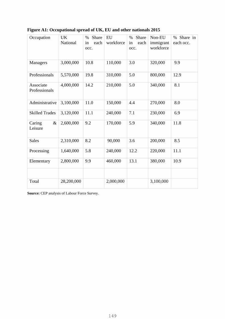
Figure A1: Occupational spread of UK, EU and other nationals 2015

Occupation UK National

% Share in each occ.

EU workforce


Non-EU immigrant workforce


Managers 3,000,000 10.8 110,000 3.0 320,000 9.9

Professionals 5,570,000 19.8 310,000 5.0 800,000 12.9

Associate Professionals

4,000,000 14.2 210,000 5.0 340,000 8.1

Administrative 3,100,000 11.0 150,000 4.4 270,000 8.0

Skilled Trades 3,120,000 11.1 240,000 7.1 230,000 6.9

Caring & Leisure

2,600,000 9.2 170,000 5.9 340,000 11.8

Sales 2,310,000 8.2 90,000 3.6 200,000 8.5

Processing 1,640,000 5.8 240,000 12.2 220,000 11.1

Elementary 2,800,000 9.9 460,000 13.1 380,000 10.9

Total 28,200,000 2,000,000 3,100,000

Source: CEP analysis of Labour Force Survey.

149

Figure A2: Real wage changes for high, middle and low earners: UK-born 2001-2015

Source: CEP analysis of Labour Force Survey. Figure A3: Changes in UK-born unemployment rate 2011-15

Source: CEP analysis of Labour Force Survey. Notes: Each dot represents a UK local authority. The solid line is the predicted ‘best fit’ from a regression of changes in unemployment on the change in share of EU immigrants in each UK local authority. These are weighted by the sample population in each area.

23

45

6%

EU

in w

orki

ng a

ge p

opul

atio

n

1.6

22.

42.

83.

23.

64

rela

tive

diffe

renc

e in

pay

1995 2000 2005 2010 2015

90:50 90:10 50:10 EU share

Wage Inequality for UK-Born Individuals 1994-2015

-10

-8-6

-4-2

02

46

810

% C

hang

e in

loca

l are

a U

nem

ploy

men

t Rat

e: 2

011-

2015

-2 0 2 4 6 8 10% Change in local area EU-Born Immigrant Share 2011-2015

local area Values Fitted Value

Change in UK-Born Unemployment Rate 2011-2015

150

Figure A4: Changes in UK-born real wages 2011-15

Source: CEP analysis of Labour Force Survey Notes: Each dot represents a UK local authority. The solid line is the predicted ‘best fit’ from a regression of local authority’s percentage change in wages on the change in share of EU immigrants. These are weighted by the sample population in each area. Figure A5: Changes in UK-born NEET rate for less skilled 2011-15

Source: CEP analysis of Labour Force Survey. Notes: Each dot represents a UK local authority. The solid line is the predicted ‘best fit’ from a regression of local authority’s changes in NEET rates for the less skilled on the change in share of EU immigrants. These are weighted by the sample population in each area. NEET stands for those ‘not in education, employment or training.’ Less skilled is defined by those who left school at 16 or earlier.

-25

-20

-15

-10

-50

510

1520

% C

hang

e in

loca

l are

a U

K-Bo

rn W

ages

: 201

1-20

15

-4 -2 0 2 4 6 8 10% Change in local area EU Immigrant Share 2011-2015


% Changes in UK-Born Real Wages: 2011-2015-2

4-2

0-1

6-1

2-8

-40

48

12%

Cha

nge

in lo

cal a

rea

UK-

born

NE

ET R

ate:

201

1-20

15

-2 0 2 4 6 8 10% Change in local area EU-Born Immigrant Share 2011-2015


Change in UK-Born NEET Rate for Less Skilled 2011-2015

151

Figure A6: Changes in real wages of UK-born less skilled 2011-15

Source: CEP analysis of Labour Force Survey. Notes: Each dot represents a UK local authority. The solid line is the predicted ‘best fit’ from a regression of local authority’s changes in the wages of the less skilled on the change in share of EU immigrants. These are weighted by the sample population in each area. Low skill is defined by those who left school at 16 or earlier. Less skilled is defined by those who left school at 16 or earlier. Figure A7: Changes in UK-born unemployment rate 2004-15

Source: CEP analysis of Labour Force Survey. Notes: Each dot represents a UK local authority. The solid line is the predicted ‘best fit’ from a regression of changes in unemployment on the change in share of EU immigrants in each UK local authority. These are weighted by the sample population in each area.

-45

-35

-25

-15

-55

1525

35%

Cha

nge

in lo

cal a

rea

UK-

Born

Wag

es: 2

011-

2015

-2 0 2 4 6 8 10% Change in local area EU Immigrant Share 2011-2015


% Changes in Real Wages of UK-Born Less Skilled: 2011-2015

152

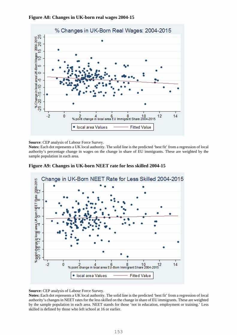
Figure A8: Changes in UK-born real wages 2004-15

Source: CEP analysis of Labour Force Survey. Notes: Each dot represents a UK local authority. The solid line is the predicted ‘best fit’ from a regression of local authority’s percentage change in wages on the change in share of EU immigrants. These are weighted by the sample population in each area. Figure A9: Changes in UK-born NEET rate for less skilled 2004-15

Source: CEP analysis of Labour Force Survey. Notes: Each dot represents a UK local authority. The solid line is the predicted ‘best fit’ from a regression of local authority’s changes in NEET rates for the less skilled on the change in share of EU immigrants. These are weighted by the sample population in each area. NEET stands for those ‘not in education, employment or training.’ Less skilled is defined by those who left school at 16 or earlier.

153

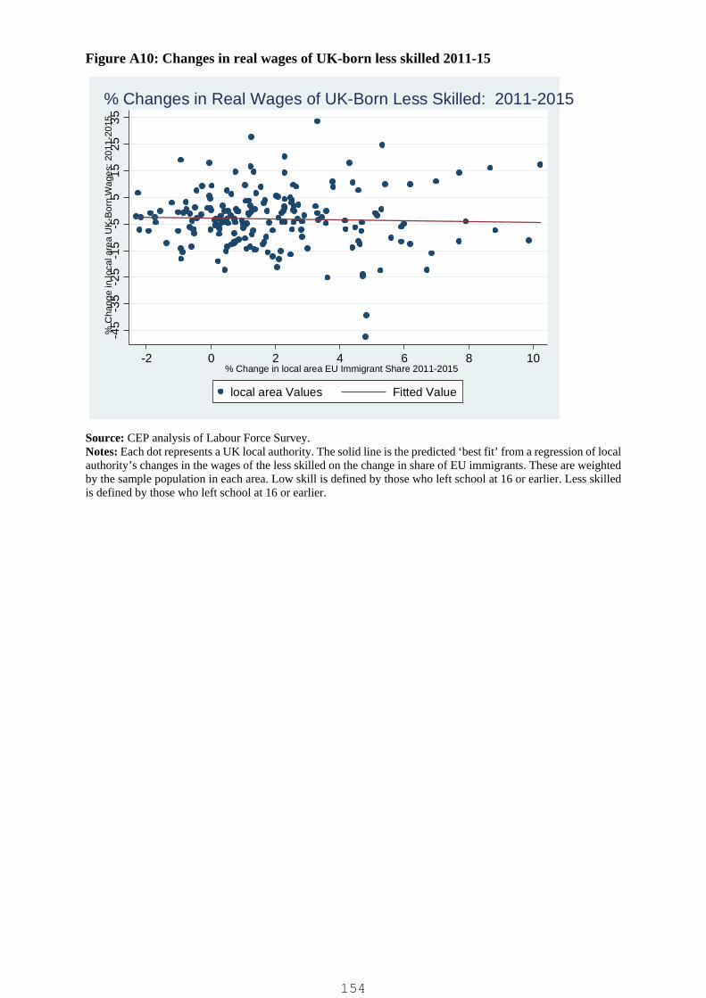
Figure A10: Changes in real wages of UK-born less skilled 2011-15

Source: CEP analysis of Labour Force Survey. Notes: Each dot represents a UK local authority. The solid line is the predicted ‘best fit’ from a regression of local authority’s changes in the wages of the less skilled on the change in share of EU immigrants. These are weighted by the sample population in each area. Low skill is defined by those who left school at 16 or earlier. Less skilled is defined by those who left school at 16 or earlier.

-45

-35

-25

-15

-55

1525

35%

Cha

nge

in lo

cal a

rea

UK

-Bor

n W

ages

: 201

1-20

15

-2 0 2 4 6 8 10% Change in local area EU Immigrant Share 2011-2015


% Changes in Real Wages of UK-Born Less Skilled: 2011-2015

154

Centre for Economic Performance

London School of Economics and Political Science

Houghton Street London WC2A 2AE UK Tel: +44(0)20 7955 7673 Email: [email protected] Twitter: @CEP_LSE

Facebook: https://www.facebook.com/centre4economicperformance


https://www.facebook.com/Centre4EconomicPerformance