Page | 1

Brewery: A Data Mining Project By Thomas Flynn, Callie Helms, Bailey Pink, and Paul Scheetz

1. Introduction

This project utilizes the data mining techniques of decision trees and neural networks to predict customer behavior given specific characteristics. More than just an application, however, this project serves as a learning experience. Our overarching goal is to gain key insights into the performance and impact of varied implementations of data mining algorithms.

1.1 Application Motivation

Business wisdom stresses the importance of an effective marketing mix: product, price, place, and promotion. Each component represents a controllable parameter, subject to internal company limitations and external industry constraints. Ultimately, a firm makes decisions to center the marketing mix on customers in its target market. Customer satisfaction and value perception reach their maximum when this goal is met.

Brewery focuses on the promotional element in the marketing mix. Developed for the Wonderful Wines of the World Company (WWWC), Brewery’s goal is to identify the market best served by the company’s new wine-tasting initiative. WWWC seeks to increase profitability and build loyalty by selecting a target market for local wine-tasting promotions cross-sold by telephone. WWWC will charge $50 to attend the wine-tasting, $25 above the event cost per customer. Inviting customers to attend costs an additional $3.20 (paid to the telemarketing firm who makes reservations). Calculations reveal at least 12.8 percent of invitees must attend to break even.

WWWC has held one test promotion for 100,000 randomly-selected customers, of whom merely 7.5 percent attended the tasting promotion. Telephoning WWWC’s entire customer base of 300,000 would thus result in a promotional loss. Clearly, only a small subset of clients is interested in the promotion. Identifying this subset will likely yield high profits—as previously mentioned, the event has a gross margin of 50 percent. Brewery’s goal is to accomplish the challenge of distinguishing the promotion’s target market.

1.2 Application Description

Seeking to determine the exact subset of customers who would accept the wine-tasting invitation, Brewery employs data mining and artificial intelligence techniques. In this context, data mining refers to the process of identifying relationships among large sets of data. Through “knowledge discovery” (discovering patterns by examining numerous cases), Brewery establishes criteria to describe customers who will undoubtedly accept invitations.

Initially, Brewery draws upon two random test samples of 100,000 database customers who were previously telephoned and invited to participate in the promotion. For these customers, the database contains an additional field to store promotional responses (“0” if did not attend, “1” if attended). From this dataset, Brewery analyzes customer demographics and response patterns using a variety of algorithms. Each algorithm creates rules to apply to the remaining 200,000 customers. These rules determine which customers will be extended an invitation. Success depends on the overall attendance

Page | 2

rate of the phoned group. Using multiple algorithms enables Brewery to generate the highest profit while providing student developers with the opportunity to explore several techniques.

1.3 Evaluating Effectiveness

As a business application, Brewery’s success will be evaluated by the profitability of the target market it selects. Identified by Dr. Allen Ball, the maximum profit is about $434,000, achieved by only inviting the exact customers who wish to attend the promotion. Real life, intelligent manual data mining by Dr. Ball typically yields a profit around $200,000. Therefore, Brewery is successful if it outperforms the typical human analysis and generates a predicted profit of more than $200,000 (Ball 2011).

1.4 Employed Techniques

1.4.1 Neural Networks

One technique we use to solve this problem is a neural network. A neural network mimics the biological neural network in humans: the system is comprised of interconnecting artificial “neurons” that make decisions. In general, there are three layers to the system: an input layer, a hidden layer and an output layer. These layers achieve a connectionist approach to computation, leading to an adaptive system that modifies itself based on new information. Specifically, the weights of the connections change in response to new data points. Neural networks are thus effective when modeling complex relationships and finding patterns in data. A main disadvantage to neural networks is that their output is not readily interpretable: the end user must employ some insight in interpretation. However, because the neural network is an adaptive technique to find patterns in data, it is an excellent solution to identify the factors influencing wine taste participation. We employ neural networks using SPSS and WEKA, explained in further detail in the Methodology and Design section.

1.4.2 Decision Trees

A second highly applicable technique to our presented problem is a decision tree. A decision tree is an algorithm that uses a tree with branches and leaves to classify data inputs. A decision tree attempts to predict outcomes based on preexisting database information comprised of specific inputs and their outputs. A tree consists of a series of nodes which represent data input. Each node has a series of children nodes, or leaves, that consist of other data inputs. A tree is “learned” recursively in a process called recursive partitioning. This process consists of separating a source sample into two separate samples based on an attribute value test. The process then continues recursively until a stopping point is reached. Once a tree is learned, the Gini Impurity test can be applied to a set of data to determine the probability of a piece of data being mislabeled. This test is used to determine the appropriate stopping point of the recursive partitioning function. Once a tree is learned, data sets can be classified with a known likelihood of correct labeling. Compared to neural networks, decision trees produce easily interpretable results: branches and decision points show the rules associated with classification. Clearly, a learned tree in this instance classifies customers who are likely to accept the promotion. Decision trees are employed using SPSS and WEKA, again explained in further detail in the Methodology and Design section.

1.4.3 Exclusion of Genetic Algorithms

Initially, we did consider using a genetic algorithm, a technique that mimics the natural world. Genetic algorithms work by first creating a set of random numbers called the population. The population is ranked and the “next generation” (new population) is created through the following process: First,

Page | 3

through a process known as elitism, the top solutions in the current population are added to the next generation. The next step in creating the next generation is to create new solutions by modifying the best existing solutions. This modification can occur by mutating, which involves randomly changing an existing solution, or breeding, in which the two best solutions are combined in some way. This is similar to survival of the fittest, in which the best continue to live another day. Through this process only the fittest solutions survive to the end. Ultimately, genetic algorithms proved too complex and time-consuming for this application. Based on our knowledge, neural networks and decision trees seem most fitting and adequate; we simply lack the domain knowledge and programming power to implement a genetic algorithm.

1.5 Justification for Artificial Intelligence

Decision tress help classify WWWC’s customers into segments—e.g., given characteristics x1, x2, …xn and a decision tree, we can say with a certain probability that the customer will accept the promotion. Neural networks operate similarly, taking in customer demographics, lifestyles, and preferences and then weighting these attributes to determine a customer’s acceptance likelihood.

Both these approaches are necessary because WWWC lacks domain expertise: ultimately, it is unknown which variables most influence customer promotional attendance. Importantly, the database is too large for WWWC to perform data mining by hand. Thus, decision trees and neural networks help WWWC learn how to classify customers given specific traits. Furthermore, these techniques allow cross-validation and reinforcement learning to better WWWC’s systems. Overall, WWWC needs a fast, efficient, accurate, and adaptive means to classify customers. Decision trees and neural networks provide all of these.

2. Background and Related Work

2.1 Data Mining Background

Before performing our own data mining, it is useful to examine existing work and gain insight. First, Olson and Dursun (2008) praise data mining’s usefulness in targeting and profiling customers. Targeting enables businesses to identify attributes of profitable customers, while profiling helps firms cluster customers into profitable segments. The pair identifies regression, neural networks, and decision trees as the most common data mining techniques. In selecting data mining tools, Olson and Dursun recommend that the tools be versatile (applicable to a wide variety of models), scalable (useful on large and small datasets), and accurate. Their book names WEKA and SPSS among the most useful data mining tools.

In support of our decision to use decision trees in WWWC’s case, the 2006 International Conference on Data Mining ranks C4.5 decision trees as the top data mining algorithm (Wu et al.). Using WEKA, we employ the C4.5 algorithm. Conference presenters praise the C4.5’s use of information gain to create decision nodes based on the attribute with the highest information gain. Additionally, automatic pruning reduces the likelihood of overfitting data. To conclude, the presenters also note that C4.5 trees do have disadvantages. Importantly, their implementation requires a large amount of CPU time and memory. In their experience, increasing records by a factor of 10 increased CPU time by a factor of 44 and rule generation by a factor of 300 (Wu et al. 2006).

Strengthening our choice of neural networks, Krieger (1996) points out their value and popularity in data mining. Neural networks are very useful because they can recognize patterns and predict functions. As

Page | 4

Krieger emphasizes, large datasets require automated processing. Krieger describes neural networks in three pieces: (1) a system of connections among nodes; (2) a method for determining the relative weights of the connections; and (3) a function for determining the ultimate outcome of a connection path. As a caveat, however, Krieger does assert that neural networks are hard to interpret and thus require expert analysis.

2.2 Data Mining Successes

As an example of successful data mining, Olson and Dursun point to Harrah’s Entertainment Inc. Harrah’s uses its Total Gold incentive cards to collect data on customer gaming behaviors, eating habits, and hotel visits. Performing data mining on records from eight million customers, Harrah’s found that 26 percent of its customers generated 82 percent of its revenues. Thus, the casino invited these select customers to special events, increasing profits.

Regarding decision trees, Gagne, McGovern, and Brotzge (2009) report their success in classification problems. The group utilized decision trees to classify weather and storm patterns. Decision tree outputs were then compared to other, more complex methods. The team chose decision trees as the main method, however, because they are easily interpretable. Their application also weighted attributes, focusing on the most important ones. One component of their study that differs from Brewery is their allowance of changing attributes groups that comprised the trees; Brewery instead modifies factors of the decision tree based on one set of unchangeable attributes. The Oklahoma team used WEKA to train their decision trees, just as Brewery does. After generating many decision trees using different groups of attribute types, they used algorithms to determine each decision tree’s validity, including the true skill statistic. Results indicate that decision trees are just as accurate in classifying storm types as other, more complicated learning algorithms. In short, there was no loss of validity in using a decision tree. Furthermore, decision trees are much easier to interpret than other techniques, proving decision trees are a very valuable classification tool (Gagne, McGovern, Brotzge 2009).

Focusing specifically on neural networks, two examples illustrate their utility. First, the IRS uses neural networks to help identify tax code noncompliance. Neural networks pinpoint the characteristics of likely noncompliance cases. By using neural networks, the IRS was able to reduce the number of database it examined from 150 to 8 (Mena 1994). In a second example, jeans company Wrangler employs neural networks to predict inventory needs given customer demand data. According to the firm, neural networks have increased sales, lowered inventory costs, and improved customer satisfaction—all of which lead to higher profits (Blanchard 1996). Clearly, neural networks improve businesses processes.

Interestingly connected to WWWC’s industry, Coors Brewers Ltd. employed neural networks to solve the issue of creating the perfect beer flavors. Offering many products with different chemical compositions satisfies more customer tastes, increasing demand for Coors. Because the relationship between chemical composition and beer flavor was unknown, Coors used database information and neural networks to link beer flavor with chemical inputs. Today, Coors still uses the neural network outputs to help in product development (Turban 2010).

3. Methodology and Design

Rather than devote our time to coding algorithms that others have already implemented, we chose to use widely available and trusted software suites. This choice shifts the focus from coding to analysis, important in developing insights. Thus, a major portion of the design was deciding which preexisting

Page | 5

tools to employ in generating our decision trees and neural networks. In selecting software, we considered three major aspects: functionality, proven success, and ease of use.

The first program we use is WEKA. WEKA is a Java software program offering a suite of machine learning algorithms for data mining. Written by developers at the University of Waikato, New Zealand, WEKA is free and open source under the GNU General Public License. In our implementation, we use the preexisting WEKA interface to apply the algorithms to our dataset (Frank, Hall, and Trig 2011).

The second program we utilize is SPSS. SPSS is a computer system that analyzes data using various analytic techniques. It is a robust system that is easy to use and fairly intuitive in its design. We had used it previously in our Marketing class, so, as a whole, the team had a base knowledge of how its operations. Additionally, excellent documentation exists on how to use SPSS when running decision trees and neural networks, valuable in completing this study.

Addressing functionality and proven success, both WEKA and SPSS have been identified as superior software suites for data mining (Olson and Dursun 2008; Ball 2011). Addressing ease of use, documentation, experience, and personal exploration led us to conclude that WEKA and SPSS are intuitive, robust software applications suitable to our needs.

3.1 Decision Trees

3.1.1 WEKA

A key benefit of WEKA is its implementation of the C4.5 algorithm for creating decision trees, especially regarding tree pruning. As identified by Wu et al. (2006), the C4.5 algorithm is extremely useful in generating accurate decision trees. The C4.5 algorithm operates as follows:

1. If base case is satisfied, end execution; else 2. For each attribute a

a. Find the information gain from splitting on a 3. Store a_best as the attribute with the highest information gain 4. Create a node that splits on a_best 5. Recursively perform the algorithm on each sublist by splitting on a_best

Missing attribute values are simply not used in information gain calculations. After the algorithm completes, automatic tree pruning ensues, reducing the likelihood of overfitting the data. Accomplished in one pass through the tree, pruning occurs bottom to top based on calculations of a leaf’s error rate given our specified confidence level. Subtrees are replaced by children nodes if the sum of their branches’ errors is higher than any of their leaf nodes (Wu et al. 2006). Overall, low confidence factors increase the amount of pruning.

Finally, another advantage of WEKA is its intuitive interface and extensive output. Parameters and testing options are easily modifiable, and program output is especially useful in Brewery. Most notably, WEKA’s confusion matrix details false positives, important in calculating overall profits, as false positives represent declined invitations.

3.1.2 SPSS

An impressive feature of SPSS is its ability to create decision trees using three different algorithms: chi-squared automatic interaction detection (CHAID), classification and regression trees (CRT), and quick, unbiased, efficient statistical tree (QUEST). While we performed exploratory testing with all algorithms,

Page | 6

our report focuses on the CHAID, as it is often used in direct marketing to segment customers and predict their behaviors, Brewery’s ultimate goal (Stone and Jacobs 2001).

Another advantage of using SPSS to create decision trees is the program’s easily readable and interpretable output. Not only does it provide a graphic decision tree, but is also outputs a large amount of other important data. Output reports include tree data such as height, number of terminal nodes, and total number of leaves. Furthermore, output also includes both risk and classification tables. These are both important factors of measuring the validity of a decision tree. The classification table is also known as a false positives table and shows the percent of the values that the decision tree classified correctly.

3.1.3 Design of the Results

While WEKA and SPSS supply much analytic data, we focus on comparing ones common to both applications. Analysis centers on varying three factors: percentage split of testing and training data, number of cross-validation folds, and the minimum number of instances required for node splits. Beyond examining common factors, we also chose one unique feature for each application. For WEKA, we focus on the program’s ability to prune trees, varying the confidence factor used in pruning. For SPSS, we focus on the confidence level necessary for splitting nodes. To evaluate results and gain insight, we analyze each implementation’s correctly classified instances and false positives table. The false positives and percent correct were also taken into account, as well as the overall size of the tree.

3.2 Neural Networks

3.2.1 WEKA

WEKA employs a multilayer perceptron network (MLPN) to create neural networks, also known as a feed-forward network. The MLPN provides a flexible model specially suited to WWWC’s limited domain knowledge. Each MLPN contains a hidden layer and hidden nodes, which allow the neural network to adjust its complexity. MLPN’s with few hidden nodes resemble polynomial regression models (Sarle 1994). The multilayer perceptron algorithm operates as follows:

1. Initialize weights and threshold 2. Present input and desired output 3. Calculate output

a. Each layer calculates output and passes to next layer 4. Adapt weights

a. Work backward from given output

WEKA is easy to use through the use of an effective user interface. Massive amounts of data are output, allowing the user to select relevant and important data. A confusion matrix is included in the output which is particularly applicable to the WWWC’s problem. The matrix can easily be segmented into false positives (customers who declined invitations) as well as true positives (customers who accepted invitations), enabling the calculation of profits for WWWC.

3.2.2 SPSS

A key benefit in the SPSS implementation of multilayer perception neural networks is the ability to select multiple dependent variable nodes and specific input nodes. This feature allows for the customization of networks to a degree which is not seen in the WEKA implementation.

Page | 7

SPSS also provides a great deal of well labeled and easy –to-interpret output tables. These tables include classification of correctly and incorrectly categorized dependent variables, a network diagram displaying input nodes, hidden nodes, output nodes, and synaptic weights, and independent variable importance details.

Unfortunately, one of the drawbacks of neural networks is the lack of folding in training. SPSS has only two training options: random selection and partition selection. Each of these training options only runs one training partition.

3.3 Presented Challenges

Data mining is a difficult process subject to potential errors. Most importantly, a system developed using a small number of instances may lose accuracy when applied to a large dataset. Being one hundred percent for the training set is likely not a reachable goal; consequently, some error is expected in our final solution. Furthermore, even if our system works perfectly on the training set, various issues may arise in applying it to the larger, perhaps more diverse database.

Importantly, our test database may not contain entirely representative data. Rules derived from the test data may not cover all attribute instances and values of the larger dataset. Thus, machine learning will be hindered. Effectiveness will also decrease due to limited information: that is, two objects with the same attribute values may have different outcomes, thwarting logic. Furthermore, our application cannot account for attributes and underlying characteristics outside the database that may be better indicators of outcome. Lacking much domain expertise, we do not know if other attributes would better classify the data. Ultimately, the application is limited by the information present in the given database.

4. Implementation

4.1 File Format

Before using WEKA or SPSS, we had to first convert the 100,000 customer listings into usable file formats for each program. A Java program parsed the customer data, converting each record to one line in a .csv file. The file was then opened in Microsoft Excel, where all missing data (indicated by periods) was replaced with a blank space, necessary for both SPSS and WEKA.

After this, we modified two times: once for WEKA and once for SPSS. SPSS modifications were fairly quick and straightforward, as data labels were simply applied. WEKA modifications, conversely, were more time-consuming and complex. WEKA requires .arff files to be formatted using specific guidelines. WEKA input files must include a relation, attribute descriptions, and perfectly formatted data rows. Portions of the SPSS and WEKA input files are included in the Appendix.

4.2 Decision Trees

We implemented and analyzed decision trees using both WEKA and SPSS, described below. Our approach was to test how each variety of tree fared compared to others. We ran a number of trees through both WEKA and SPSS, comparing the results. We modified one factor at a time and took note of the output and how each change affected the tree. Because of this method of comparison, we used one set of attributes throughout the entire process; that is, we set all variables (save the customer id) as independent variables and had the acceptance of the invitation to the wine tasting as the dependent variable.

Page | 8

Our decision tree experiments in WEKA analyze the impact of four algorithm considerations: (1) training and test dataset splits, (2) number of cross-validation folds, (3) minimum number of instances per leaf, and (4) confidence factor for pruning. Our decision tree experiments in SPSS analyze the impact of four algorithm considerations: (1) training and test dataset splits, (2) number of cross-validation folds, (3) minimum number of instances per leaf, and (4) confidence factor forsplitting. Each experiment is described in 4.2.1 and 4.2.2 below.

To analyze the impact of each experiment, we recorded tree size, number of leaves, percentage of correctly classified instances, and the confusion matrix. Our results are described in section 5.

4.2.1 WEKA

4.2.1.1 Training and Test Dataset Splits

To analyze the impact of using different dataset percentages of training and test data, we modify the

“Percentage split” option under the Test options panel. The percentage split input indicates the percent

of data that will be used as the training set. The remainder of the data is used as the test set. In our

experiments, we analyze four percentage splits: (1) 99% training set, 75% training set, 50% training set,

and 25% training set. Thus, we ran four different experiments using each of the aforementioned training

set percentages.

4.2.1.2 Number of Cross-Validation Folds

To analyze the impact of varying the number of cross-validation folds, we modify the “Cross-validation”

option under the Test options panel. In our experiments, we analyze four numbers of cross-validation

folds: 2, 5, 10, and 20. Thus, we ran four different experiments using each of the aforementioned

numbers for cross-validation folds.

4.2.1.3 Minimum Number of Instances per Leaf

To analyze the impact of changing the minimum number of instances per leaf, we modify the

“minNumObj” parameter on the parameters window. In our experiments, we analyze four values of

minimum number of instances per leaf: 2, 50, 100, and 200. Thus, we ran four different experiments

using each of the aforementioned minimum number of instances per leaf.

4.2.1.4 Confidence Factor for Pruning

To analyze the impact of altering the confidence factor using in tree pruning, we modify the “confidenceFactor” parameter on the parameters window. In our experiments, we analyze six confidence factor values: .01, .05, .1, .15, .25, and .5. Thus, we ran six different experiments using each of the aforementioned confidence factor values.

4.2.2 SPSS

4.2.2.1 Training and Test Dataset Splits

To analyze the impact of using different dataset percentages of training and test data, we modify the “Split-sample validation” option under the Validation options pane, from the main decision tree display. The percentage split input indicates the percent of data that will be used as the training set. The remainder of the data is used as the test set. In our experiments, we analyze four percentage splits: (1) 99% training set, 75% training set, 50% training set, and 25% training set. Thus, we ran four different experiments, using each of the aforementioned training set percentages.

Page | 9

4.2.2.2 Number of Cross-Validation Folds

To analyze the impact of varying the number of cross-validation folds, we modify the “Cross-validation” option under the Validation options panel. In our experiments, we analyze four numbers of cross-validation folds: 2, 5, 10, and 20. Thus, we ran four more experiments, using each of the aforementioned fold values.

4.2.2.3 Minimum Number of Instances per Leaf

To analyze the impact of changing the minimum number of instances per leaf, we modify the “Minimum Number of Cases” parameter on the Growth Limits tab of the Criteria window. In our experiments, we analyze four values of minimum number of instances per leaf: 2, 50, 100, and 200. Thus, we ran four more experiments, using each of the aforementioned minimum instance factors.

4.2.2.4 Confidence Factor

To analyze the impact of altering the confidence factor, we modify the “Significance Level For” parameter on the parameters window. In our experiments, we analyze six confidence factor values: .01, .05, .1, and .15. Thus, we ran four more experiments, using each of the aforementioned confidence factors.

4.3 Neural Networks

We implemented and analyzed multilayer perception neural networks using both WEKA and SPSS, described below. Our approach was to test how each variety of network fared compared to the other. We ran a number of networks through both WEKA and SPSS, comparing the results. We modified one factor at a time and took note of the output and how each change affected the network. Because of this method of comparison, we used one set of attributes throughout the entire process; that is, we set all variables (save the customer id) as independent variables and had the acceptance of the invitation to the wine tasting as the dependent variable.

Our neural network experiments in WEKA analyze the impact of four algorithm considerations: (1) learning rate, (2) momentum, (3) training time, and (4) training epochs. Our neural network experiments in SPSS analyze the impact of four algorithm considerations: (1) learning rate, (2) momentum, (3) training time, and (4) training epochs. Each experiment is described below.

To analyze the impact of each experiment, we recorded time taken to run algorithm, percentage of correctly classified instances, and the confusion matrix. Our results are described in section 5.

4.2.1 WEKA

4.2.1.1 Learning Rate

To determine the impact of using differing learning rates we used three different rates while keeping all other (momentum, training time, and epochs) constant. We ran this without using the GUI to allow for as little human error as possible. The different learning rates were .1, .3, and .5. For the first experiment we entered .1 in learning rate, second .2, and third .5. The constants we used for the experiment were .2 doe momentum, 10 training time, and 10 for epochs. 4.2.1.2 Momentum The next set of experiments was focused on momentum. Momentum allows for the persistence of change to the synaptic connection in following iterations. We ran this without using the GUI to allow for as little human error as possible. The variables that were held constant for these experiments were

Page | 10

learning rate at .3, training time at 10 seconds, and epochs at 10. The first experiment had momentum at .1, the second at .2, and the third at .3. 4.2.1.3 Training Time The following experiments were dedicated to training time and its effects on the network. We ran this without using the GUI to allow for as little human error as possible. The constants for these experiments were .3 learning rate, .2 momentums, and 10 epochs. The first experiment had training time set to 5 seconds, for the second 10 seconds, and 15 seconds for the final experiment.

4.2.1.4 Epochs

The final set of experiments was focused on epochs. We ran this with the GUI as it was the only way to alter the epochs. The constants for this set were .3 for a learning rate, .2 for momentum, and 10 for training time. The epochs for the first experiment were 5, for the second 10, and for the third 20.

4.2.2 SPSS

4.3.2.1 Learning Rate

To analyze the impact of using different learning rates on training data and subsequently the test data, we modify the “Learning Rate” option under the Training options pane from the main neural network display. The learning rate indicates the amount of change in each subsequent iteration in the synaptic connections of the neural network. In our experiments, we analyze three learning rates: (1) .1, .3, and .5. Thus, we ran three different experiments, using each of the respective learning rates.

4.3.2.2 Momentum

To analyze the impact of momentum on the classification of the dependent variable we modify the “momentum” option under the Training options pane from the main neural network display. The momentum indicates the persistence in the change to the synaptic connection over subsequent training iterations. In our experiments, we analyze three different momentums: (1) .1, .2, and .3. Thus, we ran three different experiments, using each of the respective momentum values.

4.3.2.3 Training Time

To analyze the impact of training time on the classification of the dependent variable, we modify the “Maximum Training Time” option under the Options pane within the main neural network display. The maximum training time is the maximum time the training is allowed to run if no other stopping condition is reached. In our experiments, we analyze three different values for maximum training time: (1) 5, 10, and 15. Thus, we ran three different experiments, using each of the respective maximum training times.

4.3.2.4 Training Epochs

To analyze the impact of training time on the classification of the dependent variable, first select “specify custom value” under “maximum training epochs” and then modify the “Maximum Training epochs” option under the Options pane within the main neural network display. The maximum training epochs is the maximum amount of training iterations the algorithm is allowed to run if no other stopping condition is reached. In our experiments, we analyze three different values for maximum training time: (1) 5, 10, and 20. Thus, we ran three different experiments, using each of the respective maximum training epochs.

Page | 11

4.4 Issues Encountered

As with any project, the team encountered challenges along the way. Our most significant issues arose with our large dataset and inexperience with the chosen software suites.

4.4.1 Dataset

In the beginning stages of the project, the team encountered considerable difficulties related to the dataset. First, just transferring the large and unwieldy dataset of 100,000 customers proved a challenge: the owner first sent a corrupted file, and then sent a file in a difficult format to interpret. After receiving a readable dataset the third time, we next had to write a file parser in Java to format entries using a base format conducive to further modifications for WEKA and SPSS, as described in 4.1.

4.4.2 WEKA and SPSS

Learning other developers’ programs is always a challenge. Much time was devoted to understanding how to input data correctly and interpret the results of both WEKA and SPSS. Fortunately, user manuals exist for both applications; unfortunately, user manuals were not always specific enough to satisfy our needs. Specifically related to WEKA, we encountered a roadblock related to computer memory recognition. WEKA did not recognize development environment memory, and thus continually ran out of heap space during execution. To remedy this, the team consulted Adam Eck, who was able to troubleshoot and solve the issue by modifying system settings in WEKA.

4.4.3 SPSS Random Training Sample

When selecting a training sample for neural networks in SPSS, the program defaults to random selection based on a randomly seeded Bernoulli distribution. The problem occurs when trying to compare outputs of neural networks trained on different datasets. A neural network with a unique training dataset will perform different on the test dataset than a neural network with a different training dataset, making it impossible to compare outputs. To circumvent this issue, we added a new variable called PARTITION to the dataset. This variable was assigned either a 1 or a 0 in each case based on a Bernoulli distribution of 30 percent. By doing so, we were able to use the same training dataset for each experiment ran in SPSS.

5. Results

5.1 Decision Trees

5.1.1 Training and Test Dataset Splits

Presentation Brewery compares and focuses on the size of the testing and training samples because it is an impactful and easily changeable factor in both WEKA and SPSS. Using a training and testing set helps predict model accuracy by running the test data (which is different from the training data) against decision rules. Correctly classified instances allude to the possibility of overfitting the training data. Key results are measured by the percent of correctly classified instances, as shown in Figure 1 on the next page.

Page | 12

Observation

WEKA’s results to this test were as we had expected. The greater the training sample, the more likely the tree was to overfit the dataset. This resulted in a lower percent correct for the number of predicted instances, although it was only a slight difference.

SPSS’s results were very different from those from WEKA. The test’s percent correct was perfect when the training set was 99 percent. There was a significant drop in the correctness between the largest training set and second largest training sets. From there, the correctness decreased slightly for every decrease in training set.

Justification

There are few reasons we believe that our results came out the way they did. It was very interesting to see that our results contradicted itself between the two programs. It would be reasonable to assume that they both would react in the same fashion, either both increase with increased training, or both decrease with increased training. However, WEKA’s results decreased with more training and SPSS’s increased with more training. Both sets of results do have some logical reasoning behind them, although it is puzzling to determine which is correct.

WEKA’s results seem to respond in the general nature of a decision tree. For one, decision trees tend to be more successful when they are smaller and more general, ensuring that the tree from the training is not overfitted to all other data. This is indeed a speculation of what happened. As the training increased, the trees became more and more fitted to that set of data, which resulted in it not fitting the test set of

Figure 1. Impact of Varying Test and Training Set Percentages

Under WEKA’s C4.5 algorithm implementation, the greater the training sample, the more likely the tree was to overfit the dataset. Conversely, since SPSS’s CHAID algorithm thrives

in large datasets, its results declined in response to lowering the training set percentage.

Page | 13

data. This would therefore result in the lessening of correctness as the training increased. Another reason for this could be the fact that WEKA prunes the decision trees, and SPSS does not. While pruning is advantageous to most data sets because it keeps the tree smaller and more generalizable. The more training, the decision tree may have been over pruned, and not as good of fit to the test dataset.

SPSS’s results acted in an opposite manner from WEKA’s. This is because it is not pruned, as WEKA’s data sets are. It is also reasonable to believe that the algorithm behind SPSS, CHAID, actually improves with more training from our results. It is an algorithm that focuses on the relationship of the dependent variables. Another reason for the success with the larger training sets is due to the fact that the CHAID algorithm thrives in large datasets. This is because it splits the data many ways by default, which is a hindrance to small datasets. It is therefore reasonable to assume that the larger training sets resulted in more efficient and better training sets, as it utilized the full functionality of the CHAID algorithm. This would therefore naturally result in a more successful testing set, explaining the perfect score of the correctness. However, this could also mean that the training set is overfitted to the given data, but it just happened to be beneficial. It is possible that when using the tree created from the large training set with another set of data, it would not perform as well.

Implication

It is reasonable to assume that both applications are successful, but have different strengths. SPSS’s algorithm is better with large data sets, which could help. When working with large specific sets, it is beneficial to use SPSS and its CHAID algorithm. WEKA’s pruning could have hindered it a bit, because our data set is very specific, when pruning helps with more general sets. In this case, less pruning could have helped maintain a higher correctness percentage.

5.1.2 Minimum Number of Instances per Leaf

Presentation Another aspect we compared was the number of folds in the cross validation compared to the percent of correctly classified instances. This was another easily changed criteria in both SPSS and WEKA, and it would be interesting to see the affect the number of folds had on each algorithm (see Figure 2 on the next page).

Observation After running a few experiments with differing numbers of folds in both WEKA and SPSS, both programs reacted in fairly similar manners. SPSS had a steady rate for each variation of folds, and WEKA’s did vary. However, WEKA’s percent correct did level out after testing the ten and twenty fold groups, which is similar to SPSS.

Justification One reason for the difference is the specificity of the programs. WEKA is much more detailed and exact in the data it outputs than SPSS. For instance, SPSS’s percent correct is rounded to the nearest one-tenth of a percent, where as WEKA goes to three decimal places. Therefore, while there are differences between the two results on this particular test, it is important to note that all of the percent correct measurements are within roughly one-tenth percent of each other; between 92.5 percent and 92.6 percent. Even though WEKA’s values do change, they are minimal. Once again, the CHAID algorithm seems to be very constant compared to C4.5 of WEKA. The tree size stays much the same, as well as the percent of instances that are correctly predicted. However, WEKA’s results are very logical and to be expected. As the number of folds increases, the number of instances

Page | 14

that get excluded from the trees decreases. Therefore, as the number of folds increases, it is natural to assume that the trees would become more accurate and increase the correctness percentage.

Implication In future use, especially when using WEKA, it is important to use an optimal amount of folds. While it may not necessarily be true or worth it to increase the number of folds drastically, finding a optimal solution is key. As is seen in our tests, using twenty folds was no more advantageous than using ten, but took more time. However, using ten folds was better than only five. With SPSS, this seems to not be as vital as criteria, especially when using the CHAID function. With a large data set, the algorithm is consistent and returns very similar data, as can be seen from our graph.

5.1.3 Minimum Number of Instances per Leaf

Presentation Brewery examines the impact of changing the minimum number of instances per leaf because it is an influential variable in both SPSS and WEKA. The minimum number of instances per leaf refers to the number of records required to create a leaf. Increasing the minimum number of instances per leaf decreases tree depth and size. Key results are measured by the percent of correctly classified instances and tree size, as shown in Figures 3 and 4 (see next page for Figure 3 and page 15 for Figure 4).

Figure 2. Impact of Modifying the Number of Cross-Validation Folds

SPSS had a steady rate for each variation of folds, and WEKA’s did vary. However, WEKA’s percent correct did level out after testing the ten and twenty fold groups, which is similar to SPSS. Overall, varying the number of cross-validation folds had

little effect on the accuracy of the decision trees.

Page | 15

Observation

Both WEKA’s and SPSS’s results were exactly as expected related to tree size. The greater the number of instances required per leaf, the smaller the number of leaves and the smaller the overall size of the tree. For WEKA, increasing the number of instances required per leaf at first increased accuracy, but this increasing accuracy seems to peak around 100 instances per leaf. For SPSS, varying the number of instances required per leaf had little effect on overall precision. Interestingly, WEKA’s tree size starts at a much higher number than SPSS—using a minimum instance number of 2 produces a tree of more than 4,500 in WEKA, while SPSS generates a tree of 105.

Justification

Our results indicate that requiring a greater number of instances per leaf produces smaller trees with fewer leaves. In WEKA, smaller trees produced more accurate classifications to a certain point—i.e., smaller trees were more generalizable to the dataset. SPSS’s utilization of the CHAID algorithm is the likely cause of its unchanging precision: since CHAID thrives in large datasets, modifying instances per leaf seems to simply affect tree size. This is supported by the fact that SPSS’s overall tree sizes remain very consistent, hovering around 100, while WEKA’s overall tree sizes fluctuate from 4,505 to 47. Clearly, decreasing instances per leaf in the C4.5 algorithm produces much more generalizable trees.

Implication

Given these results, we conclude that requiring more instances per leaf is beneficial because it creates smaller trees without sacrificing precision. For end users, it is easier and quicker to interpret smaller

Figure 3. Impact of Varying the Minimum Number of Instances per Leaf

Under WEKA’s C4.5 algorithm, the greater the number of instances per leaf, the more generalizable and accurate the decision tree was. This trend holds until about 100 instances per leaf. Using SPSS’s CHAID algorithm, altering the number of instances per leaf does not affect precision, as the CHAID algorithm is very accurate in large datasets.

Page | 16

decision trees, which contain fewer classification pathways. Thus, developers should require a large number of instances per leaf.

Figure 4. Tree Size under Various Minimum Number of Instances per Leaf

Under WEKA’s C4.5 algorithm and SPSS’s CHAID algorithm, the greater the number of instances per leaf, the smaller and thus more generalizable the tree was. The C4.5 algorithm

was impacted more than the CHAID algorithm by the minimum number of instances per leaf.

Page | 17

5.1.4 Pruning Confidence Factor

Presentation Brewery analyzes the impact of altering the pruning confidence factor because it is an impactful and easily changeable factor in WEKA. By modifying the pruning confidence factor, the number of final tree leaves and overall tree size changes. In the C4.5 algorithm, post-pruning calculates the percent of misclassifications at each decision node and propagates this error up the tree. At each decision point, the algorithm contrasts each child node’s weighted error against the misclassification error if the child nodes were pruned. Importantly, the misclassification error is an estimate and takes into consideration the confidence factor. As Drazin and Montag (n.d.) explain, “This is where the statistical notion of confidence comes into play. We take a pessimistic guess of the actual classification error based on the training data. If a given node is labeled "positive" and contains 1 positive and 1 negative (incorrectly classified) instance, its error is 50%. The actual error, however, for classifying future instances at this node could be anywhere between 28% and 72% (with a confidence factor of 0.25). Since we are pessimistic about our classifier, we assign the high error of 72%.” Thus, the higher the confidence level in our training set (meaning a high confidence factor), the less likely pruning is to occur. The lower the pruning confidence factor, the more tree pruning occurs. Key results are measured by the percent of correctly classified instances and tree size, as shown in Figures 5 and 6 (see next page for Figure 6).

Figure 5. Impact of Modifying Pruning Confidence Factor

Varying the size of the pruning confidence factor in general decreases the precision of the decision tree. This is because large confidence factors discourage pruning, creating less generalizable decision trees.

Page | 18

Observation

WEKA’s results were exactly as expected. The greater the confidence factor, the less tree pruning occurred. This is represented by both tree size and number of terminal nodes: As the confidence factor increased, both tree size and terminal nodes increased. The number of correctly classified instances also varied with the confidence factor and amount of tree pruning. Interestingly, the best results were obtained with the most pruning, when the confidence factor was low. However, it is important to note that the percentage of correctly classified instances varied little.

Justification

Our results indicate that larger trees, which undergo less pruning, are slightly less accurate than heavily pruned smaller trees. Intuitively, larger trees are more specific, increasing the likelihood that they overfit the training data. Trees that undergo more pruning, and are thus smaller and contain fewer classification rules, are more generalizable to new, untested data.

Implication

Given these results, we conclude that more tree pruning (implying a low confidence factor) is advantageous for two reasons: (1) smaller trees are more generalizable to new, untested data, and (2) smaller trees are much easier to interpret as an end user. Thus, in implementing decision trees, it is wise to employ an algorithm that prunes the tree.

Figure 6. Tree Sizes under Various Pruning Confidence Factors

As expected, increasing the confidence factor discouraged tree pruning, leading to a

greater number of terminal nodes (leaves) and larger overall tree sizes.

Page | 19

Figure 8. Impact of Varying Learning Rate

As learning rate increases from .1 to .3, overall percentage of correctly classified cases increases. However, as learning rate continues to increase from .3 to .5, the overall

percentage of correctly classified cases decreases.

92.00

92.20

92.40

92.60

92.80

93.00

93.20

.1 LR .3 LR .5 LR

PEr

cen

tage

of C

ase

s C

orr

ect

ly

Cla

ssif

ied

Comparison of Changing Learning Rates in SPSS and WEKA MLP Neural Network Algorithms

SPSS

WEKA

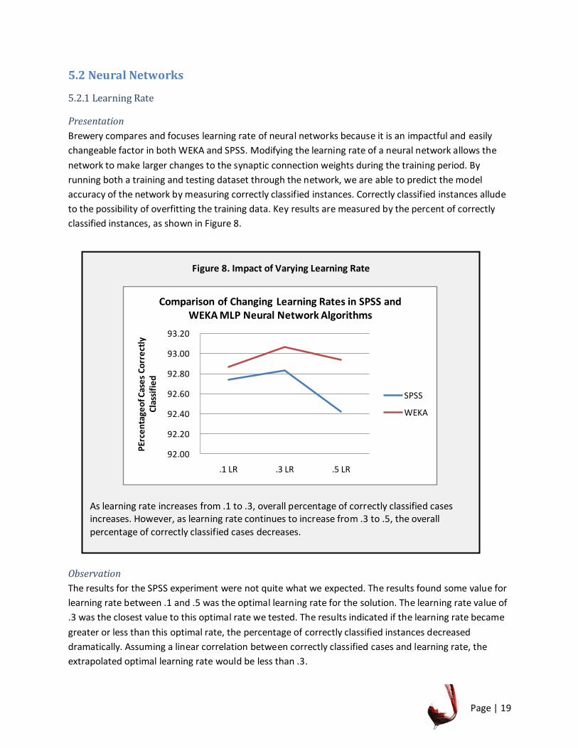
5.2 Neural Networks

5.2.1 Learning Rate

Presentation

Brewery compares and focuses learning rate of neural networks because it is an impactful and easily

changeable factor in both WEKA and SPSS. Modifying the learning rate of a neural network allows the

network to make larger changes to the synaptic connection weights during the training period. By

running both a training and testing dataset through the network, we are able to predict the model

accuracy of the network by measuring correctly classified instances. Correctly classified instances allude

to the possibility of overfitting the training data. Key results are measured by the percent of correctly

classified instances, as shown in Figure 8.

Observation

The results for the SPSS experiment were not quite what we expected. The results found some value for

learning rate between .1 and .5 was the optimal learning rate for the solution. The learning rate value of

.3 was the closest value to this optimal rate we tested. The results indicated if the learning rate became

greater or less than this optimal rate, the percentage of correctly classified instances decreased

dramatically. Assuming a linear correlation between correctly classified cases and learning rate, the

extrapolated optimal learning rate would be less than .3.

Page | 20

Similar to the results of the SPSS experiment, the results of the WEKA experiment were not quite what

we expected. The results of the WEKA experiment confirmed the observations made in the SPSS

experiment, that the optimal learning rate was somewhere between .1 and .5 for the data set. Again, .3

was the closest value we tested to the learning rate. However, unlike SPSS, the extrapolated value of the

optimal learning rate would be greater than .3.

Justification

There are a few reasons as to the difference in the optimal learning rate between the two programs. The

major potential reason as to what caused the difference is the possible difference in training sample

data sets.

In SPSS, the training data set allows for partitioning randomly or along a specified variable. In our initial

setup we created a partition variable based on a 30 percent Bernoulli distribution along all the cases.

This simply means 30 percent of the cases were assigned to the training set while 70 were assigned to

the testing set. This allowed us to keep the same training set across all SPSS experiments consistent.

However, WEKA has no method of assigning a specified training set. WEKA uses a random number

generator with different seeds for each separate experiment. As a result, WEKA’s results are more

representative of the dataset as a whole, but difficult to compare.

This issue in different training sets could be the possible reason the optimal learning rate value is

different between the two experiments.

Implications

It is reasonable to assume both algorithms were successful in their experimental runs. However, it is

difficult to compare the two results directly because of the differences in training sets. It is reasonable to

also assume both algorithms have different strengths. SPSS’s strength in this experiment is the ability to

have a consistent training dataset across multiple experiments, while WEKA’s strength lies in its ability

to reduce sampling error in experiments, thereby giving it more precise results.

One thing we can imply from the results section is the presence of an optimal learning rate for this

specific data set. If the learning rate is below the optimal rate, the network does not learn fast enough

to be entirely efficient. Likewise, if the learning rate is above the optimal rate, it causes oscillations in

the synaptic weight connections because it overcorrects for incorrect categorizations.

5.2.2 Momentum

Presentation

Brewery compares and focuses on the momentum of neural networks because it is an impactful and

easily changeable factor in both WEKA and SPSS. Modifying the momentum of a neural network allows

for a change in synaptic connections to persist through later neural network training iterations. By

running both a training and testing dataset through the network, we are able to predict the model

accuracy of the network by measuring correctly classified instances. Correctly classified instances allude

to the possibility of overfitting the training data. Key results are measured by the percent of correctly

classified instances, as shown in Figure 8.

Page | 21

Figure 8. Impact of Varying Momentum

As momentum increases from .1 to .3, overall percentage of correctly classified cases increases. However, as momentum continues to increase from .3 to .5, the overall

percentage of correctly classified cases decreases.

92.00

92.20

92.40

92.60

92.80

93.00

93.20

.1 LR .3 LR .5 LR

Pe

rce

nta

geo

f Cas

es

Co

rre

ctly

C

lass

ifie

d

Comparison of Changing Learning Rates in SPSS and WEKA MLP Neural Network Algorithms

SPSS

WEKA

Observations

The results for the SPSS experiment were not quite what we expected. The results found some value for

momentum between .1 and .3 was the optimal momentum rate for the solution. The momentum value

of .2 was the closest value to this optimal rate we tested. The results indicated if the momentum

became greater or less than this optimal rate, the percentage of correctly classified instances decreased

dramatically. Assuming a linear correlation between correctly classified cases and momentum, the

extrapolated optimal momentum would be less than .2.

Similar to the results of the SPSS experiment, the results of the WEKA experiment were not quite what

we expected. The results of the WEKA experiment confirmed the observations made in the SPSS

experiment, that the optimal momentum was somewhere between .1 and .3 for the data set. Again, .2

was the closest value we tested to the optimal momentum. However, unlike SPSS, the extrapolated

value of the optimal learning rate would be less than .2.

Justification

Just as in the learning rate experiment, the major potential reason as to what caused the difference is

the possible difference in training sample data sets.

In SPSS, the training data set allows for partitioning randomly or along a specified variable. In our initial

setup we created a partition variable based on a 30 percent Bernoulli distribution along all the cases.

Page | 22

This simply means 30 percent of the cases were assigned to the training set while 70 were assigned to

the testing set. This allowed us to keep the same training set across all SPSS experiments consistent.

However, WEKA has no method of assigning a specified training set. WEKA uses a random number

generator with different seeds for each separate experiment. As a result, WEKA’s results are more

representative of the dataset as a whole, but difficult to compare.

This issue in different training sets could be the possible reason the optimal momentum value is

different between the two experiments.

Implications

Again, it is reasonable to assume both algorithms were successful in their experimental runs. Likewise, it

is reasonable to assume both algorithms have different strengths. However, it is difficult to compare the

two results directly because of the differences in training sets SPSS’s strength in this experiment is the

ability to have a consistent training dataset across multiple experiments, while WEKA’s strength lies in

its ability to reduce sampling error in experiments, thereby giving it more precise results.

One thing we can imply from the results section is the presence of an optimal momentum for this

specific data set. If the momentum is below the optimal rate, the change in synaptic weight is not

carried over and the neural network is not sufficiently trained. On the other hand, if the momentum is

above the optimal rate, the change in synaptic weights is persisted too much and the neural network is

overtrained.

5.2.3 Training Time

Presentation Brewery compares and focuses on the amount of time dedicated to training because it is an impactful and easily changeable factor in both WEKA and SPSS. The amount of time dedicated to training is how long the system is fed teaching patterns and allowed to change weights. Key results are measured by the percent of correctly classified instances, as shown in Figure 9 on the next page.

Observation

Contrary to popular belief the shorter the training time the better, at least for this set of data. For both SPSS and WEKA the results are best when the training time is the lowest. Another noteworthy observation is that both experience a major drop between the five to ten second marks. After this point both systems improve. WEKA is consistently performing more accurately than SPSS, however, it takes minutes to run while SPSS only takes a matter of seconds.

Page | 23

Justification

There are few reasons we believe that our results came out the way they did. It was very interesting to see that our results contradicted itself showing both declining and improving accuracy as time increased. It would be reasonable to assume as training time increases the results would react consistently, either both increase with increased training time, or both decrease with increased training time. WEKA’s results were more stable while SPSS’s was volatile.

The trend of the graph is not justifiable. There are two possible situations to indicate what happens. Both, however, are disproven due to the graphs trend. From the five second to ten second mark the accuracy decreases. This could be due to over fitting of our neural network to the data points. This can’t be the case, however, because the increase that occurs between the ten and fifteen second marks. The other possibility was that as training time increases the neural network is better able to adapt to the training set provided. This is supported by the increase in accuracy from ten to fifteen seconds but contradicted by the five to ten second data. With inconsistent results we are not able to determine which situation will improve accuracy.

The difference in volatility on the other hand is easier to explain. WEKA was much more stable as it stayed within .045% regardless of the training time. SPSS on the other hand varied .12%, over two and a half more times than WEKA. For our programs we selected the option of using a training set. This training set did not allow for the user to pick what the training set would be. The difference in volatility would indicate a difference in either size of the training set or even a difference in the quality of the training set. The larger a training set the more instances it has to learn from indicating more accuracy. The size would be irrelevant if there was poor quality. Quality would signify sufficient amounts of both positive dependent variables as well as negative.

Figure 9. Impact of Varying Training Times

Both in SPSS and in WEKA there was a dip in percent correct as time extended from 5 to

10 seconds. They both improved after that point.

Page | 24

Implication

It is reasonable to assume that both applications are consistent, but differ in volatility. Further research would need to be conducted in order to explain the trend between training times and accuracy. The training set has a large effect on overall accuracy and is vital for a successful neural network, regardless of the program used to generate it.

5.2.4 Epochs

Presentation Brewery compares and focuses on the effect the number of epochs has because it is an impactful and easily changeable factor in both WEKA and SPSS. Epochs are the number of iterations the program will go through. With each epoch the neural network is affected by performing specified algorithms one more time. Key results are measured by the percent of correctly classified instances, as shown in Figure 10.

Observation

SPSS’s results to this test were as we had expected. The greater the epochs, the more refined the neural network would be. This resulted higher accuracy as the number of epochs increased.

WEKA’s results varied greatly from SPSS. There was a negative relationship between the number of epochs and accuracy when looking at experimenting with five epochs then moving to ten. There was an increase in correctness between ten epochs and 15. Regardless of the trends WEKA remained more accurate throughout.

Figure 10. Impact of Varying Epochs

In SPSS, the greater the number of epochs, the more precise the results. Conversely, WEKA

had a drop between the first five to ten epochs, recovering between 10 and 15 epochs.

20

Page | 25

Justification

There are few reasons we believe that our results came out the way they did. It was very interesting to see that our results contradicted itself between the two programs. It would be reasonable to assume that they both would react in the same fashion, either both increasing throughout, or both decreasing. SPSS followed this logic; however, WEKA was not as consistent. It is difficult to determine why these programs reacted inconsistently.

SPSS results trended nicely. It showed that as the number of epochs the program progresses through the more accurate the data becomes overall. This makes sense as each time the program iterates through the multilayer perception algorithm it should be able to refine its weights. SPSS showed an increase in accuracy of over .5% while shifting from five to 15 epochs.

Alternatively, WEKA did not follow any trends. As WEKA increased epochs from five to ten the accuracy decreased. Then while increasing from ten to fifteen epochs the accuracy increased past the accuracy found at five epochs. This trend is contradictory in nature and shows no correlation. Since a decrease occurred between five and ten it is natural to assume this data might be over fitted to the training set. However, the increase between ten and fifteen indicates that assumption is false. The data between five epochs and ten indicates that the refining of weight as the number of epochs increase is also false.

Implication

It is reasonable to assume that both applications are successful, both consistently over 92% accuracy. SPSS acts as predicted and increasing epochs result in increased accuracy. WEKA does not react in a predictable fashion and will need more testing to determine the correct trend.

5.3 WWWC’s Profitability

Our data mining focused solely on maximizing the customer acceptance rate, assuming that invitational precision would lead to the highest profitability. For all experiments, the minimum response rate was 92 percent, much higher than any data mining performed by human analysis. In fact, most human analysis resulted in acceptance rates of 30 to 40 percent (Ball 2011). At first, Brewery’s higher acceptance rate seems best for a firm; however, running the best classification through profit analysis yielded an expected profit of just $134,055, much less than the $200,000 plus obtained through data mining by hand (see Figure 11). Brewery’s best result was obtained using a C4.5 decision tree with the following features: 50 percent training data/50 percent test data; 10 cross-validation folds; .05 confidence factor in pruning; and 100 minimum instances per leaf. The tree’s overall size was 79 with 40 leaves.

Why did our data mining yield low profitability? Simply put, maximizing response rate does maximize profit. Under most of our classifications, we invite around 4 percent of the customers to attend the wine promotion. Thus, we err on the side of not inviting people, significantly decreasing the number of false positives. Since Brewery was so accurate, it sacrificed any risk of inviting a customer who would not attend. In the promotional scheme, however, to remain profitable only one out of every eight people needed to attend the event to break even. Thus, a high ratio of false positives to true positives would have been acceptable. Brewery should have supported more risk, extending more invitations: again, for every eight invitees, if more than one person accepts, profits are achieved. Upon reflection, Brewery’s neural networks and decision trees are most favorable and better suited to situations where low risk is necessary.

Page | 26

Figure 11. Highest Profitability Achieved by Brewery

Overall, Brewery produces an expected profit of $158,055. Using the confusion matrix of the decision tree, 4.1 percent of customers will be invited (1309 + 732 divided by 50,000). We apply this projection to the entire customer database of 300,000, as taught by Dr. Ball (2011). We calculate invitational expense to be $3.20 times 12,300 invitees. The percent of true positives is the response rate achieved (1309 divided by 1309 + 732). We multiply the response rate by the number of invitations to obtain total attendees. Multiplying total attendees by gross profit per customer yields gross profit. Overall profit

is calculated as gross profit minus promotional costs.

6. Extensions and Future Work

Future Experiments One major part in our experiments was the lack of ability to test the profitability of our solutions in an easy to use and intuitive manner. When first presented with this problem, we knew that it was unrealistic that data mining alone would be able to give us the best, most profitable solutions (Ball, 2011). The results from our decision trees and neural network solutions simply gave us the best response rates, which did not necessarily mean the most revenues for WWWC. Figuring out how to not only mine the data for a good correctness percentage of people invited to the wine tasting, but also maximizing profits will be an interesting challenge that could be explored in the future.

Some other, more specific extensions and applications could be to look at the effects of using other algorithms to build the decision trees. SPSS alone had 3 other growing methods that we only tested in a limited fashion. To be more in depth about these tests and how they affect the data mining would be another useful extension of our project. To continue in that manner, it would also be interesting to see what other factors change the decision tree’s validity, such as tree depths, or using the Likelihood ratio instead of Pearson for the chi-square statistic. There is also the option of testing the attributes that included in each decision tree, to see what affect that might have on the end result.

Number of customers in entire population 300,000

Percent we will invite by telephone (target) 4.10% Total number who will receive an invitation 12300

Cost of each telephone invitation $3.20

Total cost of telephone promotion $39,360

Total costs $39,360

Response rate 64.20% Total number of responses 7,897

Gross profit each response $25.00

Total gross profit $197,415

Net profit after promotional costs $158,055

Page | 27

It would also be important to test other data sets in the future. Our results could be specific just to this data set, which could hinder the conclusions that we took away from running these experiments. It is possible that other data sets will be less fitted to our testing techniques, or may show some trends that were not seen in our WWWC testing.

Future Applications and Extensions It is clear that data mining is very important to many fields, and can be aided greatly by using AI techniques such as decision trees and neural networks. With large data sets, as is seen in our example with WWWC, trying to find patterns and trends by hand can be tedious and neigh impossible. There needs to be automation of some sort involved. It so happens that our AI applications bring other, more crucial advantages to the table as well. Their learning capabilities can result in a much more successful result than other data mining techniques, such as regression. With this being said, applications such as the ones we used are very useful in many areas, and will continue to be so in the future. Markets can be analyzed easily and efficiently in this manner, a vital undertaking of any business wishing to succeed.

Other future uses can be drawn from some that were touched on in our articles. Decision trees are used for their classifying expertise, and have been used for things such as analyzing weather patterns very successfully. Similar projects can be done to create a greater understanding of the world around us. Decision trees are great for making predictive models, as well as helping with multistage decisions. Neural networks are also very practical for classification problems. They are being put to use in the electricity industry as well as the mining industry. These applications increase efficiency and safety in both of those fields. Many other applications will appear as technology and knowledge bases grow.

7. Conclusion Overall, performance of the two algorithms varied. It is difficult to compare the two algorithms from a performance standpoint because we may not have achieved optimal training values and identical training sets. However, one comparison that is easy to make is the comparison from a user applicability perspective. The biggest difference from a practicality standpoint between the two methods is the ability to interpret the architecture and apply it to classifications. A decision tree has specific decisions that are made when classifying the data. After a decision tree is created, it generates a collection of classification rules. These rules are readable and can be practically applied to a business model in order to classify data. Neural networks function as a black box. When data is run through a neural network, it passes through and comes out the other side classified. Because of the incredible amount of synaptic connections within the hidden layer of the neural network, it is very difficult to divine any sort of practical rule to classify data.

If Brewery were implemented, decision trees would be the ideal method to use because it is easier to interpret and truly act upon their results. Neural networks provide a list of weights that are appropriate for classifying instances, but they do not provide actionable output. Overall, WWWC should utilize the decision tree classifications and consider these findings in its human analysis, focusing on maximizing both response rate and profitability.

Page | 28

References

Blanchard, David. "Wrangler Replenishes with Neural Networks." Intelligent Systems Report (1996).

Web. <http://www.lionhrtpub.com/orms/orms-2-96/cuttingedge.html>.

Ball, Dr. Allen Dwayne. Personal interview. 15 Mar. 2011.

"Definition: CHAID - TheMeasurementGroup.com." The Measurement Group. Web. 05 May 2011.

<http://www.themeasurementgroup.com/definitions/chaid.htm>.

Drazin, Sam, and Matt Montag. Decision Tree Analysis Using Weka. Publication. University of Miami.

Print.

Frank, Eibe, Mark Hall, and Len Trig. "Weka 3 - Data Mining with Open Source Machine Learning

Software in Java." Weka 3: Data Mining Software in Java. Computer Science Department,

University of Waikato, 2011. Web. <http://www.cs.waikato.ac.nz/ml/weka/>.

Gagne II, David J., Amy McGovern, and Jerry Brotzge. "Classification of Convective Areas Using Decision

Trees." American Meteorological Society 26.7 (2009). AMS Journals Online. 1 Feb. 2011. Web.

<http://journals.ametsoc.org/doi/full/10.1175/2008JTECHA1205.1>.

Krieger, Cynthia. "Neural Networks in Data Mining." University of Massachusetts Lowell, 1996. Web.

<http://www.cs.uml.edu/~ckrieger/user/Neural_Networks.pdf>.

Mena, J.“The adaptive tax collector; AI modeling tools are helping the Internal Revenue

Olson, David Louis., and Dursun Delen. Advanced Data Mining Techniques. Berlin: Springer, 2008. Print.

Sarle, Warren S. “Neural Networks and Statistical Models,” Proceedings of the Nineteenth Annual SAS

Users Group International Conference (1994): 1-13. Print.

Service detect fraud, reduce risk, and improve collections.” AI Expert (1994). Print.

Stone, Bob, and Ron Jacobs. Successful Direct Marketing Methods. Chicago, IL: McGraw-Hill, 2001. Print.

Turban, Efraim. Business Intelligence: a Managerial Approach. Upper Saddle River, NJ: Pearson Prentice

Hall, 2010. Print.

Page | 29

Wu, Xindong, Vipin Kumar, J. Ross Quinlan, Joydeep Ghosh, Qiang Yang, Hiroshi Motoda, Geoffrey J.

McLachlan, Angus Ng, Bing Liu, Philip S. Yu, Zhi-Hua Zhou, Michael Steinbach, David J. Hand, and

Dan Steinberg. "Top 10 Algorithms in Data Mining." Knowledge and Information Systems 14.1

(2008): 1-37. SpringerLink. Web. <http://www.springerlink.com/content/

08x148q7kj035542/fulltext.pdf>.

Page | 30

Appendix

Program Instructions For information on how to perform our experiments, refer to the WEKA and SPSS Instruction Manuals produced by our group.

Results/Outputs/Graphs Not Included in Results

WEKA Decision Tree Experiments

Training %

Test %

Cross-Validation #Folds

Confidence Factor

Minimum number of instances per leaf

Number of Leaves

Size of the tree

% of Correctly Classified Instances

False Positives table (L to R, top to bottom)

Experiments with Training and Test Set Percents

99 1 10 0.25 200 24 47 92.30% 24, 62, 15, 899

75 25 10 0.25 200 24 47 92.53% 1484, 4685, 921, 67910

50 50 10 0.25 200 24 47 92.61% 2406, 5915, 1472, 90207

25 75 10 0.25 200 24 47 92.76% 623, 1446, 365, 22566

Experiment with Minimum Number of Instances

50 50 10 0.05 2 2253 4505 91.69% 1567, 2583, 1571, 44279

50 50 10 0.05 50 88 175 92.79% 1274, 2876, 730, 45120

50 50 10 0.05 100 40 79 92.85% 1309, 2841, 732, 45118

50 50 10 0.05 200 24 47 92.68% 1059, 3091, 570, 45280

Experiment with Number of Folds

50 50 2 0.25 200 24 47 92.59% 2285, 6036, 1377, 90302

50 50 5 0.25 200 24 47 92.56% 2496, 5825, 1619, 90060

50 50 10 0.25 200 24 47 92.61% 2406, 5915, 1472, 90207

50 50 20 0.25 200 24 47 92.61% 2397, 5924, 1385, 90294

Experiment with Pruning Confidence Factor

50 50 10 0.01 200 15 29 92.674% 956, 3194, 469, 45381

50 50 10 0.05 200 15 29 92.673% 956, 3194, 469, 45381

Page | 31

50 50 10 0.1 200 19 37 92.678% 1059, 3091, 570, 45820

50 50 10 0.15 200 24 47 92.677% 1059, 3091, 570, 45820

50 50 10 0.25 200 24 47 92.677% 1059, 3091, 570, 45820

50 50 10 0.5 200 34 67 92.660% 1303, 2847, 823, 45027

SPSS Decision Tree Experiments

Test %

Cross-Validation #Folds

Significance Level

Minimum for Node

Number of Leaves

Size of the tree

% Correct

0 10 0.05 100 61 99 100%

25 10 0.05 100 62 99 92.80%

50 10 0.05 100 61 99 92.50%

75 10 0.05 100 44 73 92.50%

50 0 0.05 100 61 99 92.50%

50 5 0.05 100 61 99 92.50%

50 10 0.005 100 61 99 92.50%

50 20 0.05 100 61 99 92.50%

50 10 0.01 100 56 91 92.50%

50 10 0.05 100 61 99 92.50%

50 10 0.1 100 61 99 92.50%

50 10 0.15 100 61 99 92.50%

50 10 0.05 2 66 105 92.50%

50 10 0.05 50 63 101 92.50%

50 10 0.05 100 61 99 92.50%

50 10 0.05 200 59 96 92.50%

WEKA Neural Network Experiments

Learning Rate

Momentum Training Time

Epochs Time Percent Correct

False Positives table (L to R, top to bottom)

Learning Rate Experiments

0.1 0.2 10 10 270.85 93.07 a b <-- classified as

2409 5912 | a = accepted

Page | 32

1018 90661 | b = declined

0.3 0.2 10 10 267.99 92.866 a b <-- classified as

2043 6278 | a = accepted

856 90823 | b = declined

0.5 0.2 10 10 267.68 92.938 a b <-- classified as

2145 6176 | a = accepted

886 90793 | b = declined

Momentum Experiments

0.3 0.1 10 10 241.96 92.946 a b <-- classified as

2373 5948 | a = accepted

1106 90573 | b = declined

0.3 0.2 10 10 267.99 92.866 a b <-- classified as

2043 6278 | a = accepted

856 90823 | b = declined

0.3 0.3 10 10 243.53 92.851 a b <-- classified as

2020 6301 | a = accepted

848 90831 | b = declined

Training Time Experiments

0.3 0.2 5 10 142.24 92.911 a b <-- classified as

2494 5827 | a = accepted

1262 90417 | b = declined

0.3 0.2 10 10 267.99 92.866 a b <-- classified as

2043 6278 | a = accepted

856 90823 | b = declined

0.3 0.2 15 10 400.87 92.872 a b <-- classified as

2070 6251 | a = accepted

877 90802 | b = declined

Epochs Experiments

0.3 0.2 10 5 205.49 92.911 a b <-- classified as

2494 5827 | a = accepted

1262 90417 | b = declined

0.3 0.2 10 10 436.71 92.866 a b <-- classified as

2043 6278 | a = accepted

856 90823 | b = declined

0.3 0.2 10 20 763.76 92.987 a b <-- classified as

2356 5965 | a = accepted

1048 90631 | b = declined

Page | 33

SPSS Neural Network Experiments

Learning Rate

Momentum Training Time

Epochs Time Percent Correct

False Positives table (L to R, top to bottom)

Learning Rate Experiments

0.3 0.2 10 10 12.73 92.74% a b <-- classified as

3679, 4642 | a = accepted

2566, 89113 | b = declined

0.1 0.2 10 10 10.75 92.83% a b <-- classified as

3820, 4501 | a = accepted

2611, 89068 | b = declined

0.5 0.2 10 10 9.25 92.42% a b <-- classified as

3679, 4642 | a = accepted

2566, 89113 | b = declined

Momentum Experiments

0.3 0.1 10 10 13.05 92.72% a b <-- classified as

4013, 4308 | a = accepted

2883, 88796 | b = declined

0.3 0.2 10 10 12.73 92.74% a b <-- classified as

3679, 4642 | a = accepted

2566, 89113 | b = declined

0.3 0.3 10 10 9.83 92.50% a b <-- classified as

2830, 5491 | a = accepted

1926, 89753 | b = declined

Training Time Experiments

0.3 0.2 5 10 10.69 92.86% a b <-- classified as

3855, 4466 | a = accepted

2615, 89064 | b = declined

0.3 0.2 10 10 12.73 92.74% a b <-- classified as

3679, 4642 | a = accepted

2566, 89113 | b = declined

0.3 0.2 15 10 8.92 92.82% a b <-- classified as

4066, 4255 | a = accepted

2843, 88836 | b = declined

Page | 34

Printout of Programs

Neural Network Output

Because neural networks are highly complex, a typical program output spans 100+ pages. Thus, in the interests of space, this output has been excluded from our report. However, it is available upon request.

Sample WEKA Decision Tree Output

This output from WEKA is from a run with 50% training set data, 50% test set data. The pruning

confidence factor was 0.25, and the minimum number of instances per leaf was 200.

=== Run information === Scheme: weka.classifiers.trees.J48 -C 0.25 -M 200 Relation: test_weka Instances: 100000 Attributes: 68 age agegrp1 agegrp2 agegrp3 agegrp4 agegrp5 agegrp6 sex educ income incgrp1 incgrp2 incgrp3 incgrp4 incgrp5 incgrp6 kidhome teenhome gourmag winemag stylmag housmag sprtmag travmag cultmag compmag firstpur lastpur npurch tbottles totcat totcrev

Page | 35

totccost totcprof rev1styr revlstyr costlast ltv probstay avgpurch avgdisc avgqual percweb percdr percsr percdw percsw percde percex totlcomp datelate totlwrng datewrng totpcomm datelike winelovr wineknow compknow knowalt status parties travel cultural satiswww trustwww valuewww loyalwww winetast Test mode: split 50.0% train, remainder test === Classifier model (full training set) === J48 pruned tree ------------------ winemag <= 1 | costlast <= 3329912: declined (73496.0/1939.0) | costlast > 3329912 | | winemag <= 0: declined (3776.0/188.0) | | winemag > 0

Page | 36

| | | totccost <= 38769975: declined (8472.0/1529.0) | | | totccost > 38769975 | | | | housmag <= 0: declined (385.0/132.0) | | | | housmag > 0 | | | | | ltv <= 187000000000: declined (209.0/83.0) | | | | | ltv > 187000000000: accepted (217.0/78.0) winemag > 1 | kidhome <= 0 | | teenhome <= 0 | | | costlast <= 9909999 | | | | gourmag <= 1 | | | | | avgqual <= 91: declined (496.0/53.0) | | | | | avgqual > 91 | | | | | | parties <= 4: declined (247.0/33.0) | | | | | | parties > 4 | | | | | | | educ <= 14 | | | | | | | | housmag <= 0: declined (299.0/132.0) | | | | | | | | housmag > 0: accepted (210.0/73.0) | | | | | | | educ > 14 | | | | | | | | housmag <= 0: declined (2688.0/657.0) | | | | | | | | housmag > 0 | | | | | | | | | sex <= 0: accepted (339.0/153.0) | | | | | | | | | sex > 0: declined (1209.0/437.0) | | | | gourmag > 1 | | | | | educ <= 14: accepted (237.0/52.0) | | | | | educ > 14 | | | | | | cultmag <= 1 | | | | | | | housmag <= 0 | | | | | | | | ltv <= 301000000000: declined (395.0/164.0) | | | | | | | | ltv > 301000000000: accepted (441.0/193.0) | | | | | | | housmag > 0: accepted (855.0/326.0) | | | | | | cultmag > 1: declined (494.0/200.0) | | | costlast > 9909999 | | | | gourmag <= 1 | | | | | cultmag <= 0: accepted (264.0/81.0) | | | | | cultmag > 0 | | | | | | avgqual <= 990000000000: declined (212.0/84.0) | | | | | | avgqual > 990000000000: accepted (354.0/150.0) | | | | gourmag > 1: accepted (992.0/242.0) | | teenhome > 0: declined (1379.0/113.0) | kidhome > 0: declined (2334.0/16.0) Number of Leaves : 24 Size of the tree : 47 Time taken to build model: 67.37 seconds

Page | 37

=== Evaluation on test split === === Summary === Correctly Classified Instances 46339 92.678 % Incorrectly Classified Instances 3661 7.322 % Kappa statistic 0.3354 Mean absolute error 0.1202 Root mean squared error 0.2441 Relative absolute error 78.8038 % Root relative squared error 88.4724 % Total Number of Instances 50000 === Detailed Accuracy By Class === TP Rate FP Rate Precision Recall F-Measure ROC Area Class 0.255 0.012 0.65 0.255 0.366 0.739 accepted 0.988 0.745 0.936 0.988 0.961 0.739 declined Weighted Avg. 0.927 0.684 0.912 0.927 0.912 0.739 === Confusion Matrix === a b <-- classified as 1059 3091 | a = accepted 570 45280 | b = declined

Page | 38

Sample SPSS Decision Tree Output

This is sample output for the default decision tree created in SPSS. It has no validation, a maximum

depth of 3, and minimum cases in parent nodes of 100.

Page | 39

The above is an enlarged portion of the decision tree that was outputted, as seen above.