brane dynamics from the rst law of entanglement
TRANSCRIPT
Prepared for submission to JHEP
Brane dynamics from the first law of entanglement
Sean Cooper,a Dominik Neuenfeld,a,b Moshe Rozali,a David Wakehama
aDepartment of Physics and Astronomy,
University of British Columbia, 6224 Agricultural Road, Vancouver, BC V6T 0C2, CanadabPerimeter Institute for Theoretical Physics,
31 Caroline Street N., Waterloo, Ontario N2L 2Y5, Canada
E-mail: [email protected], [email protected],
[email protected], [email protected]
Abstract: In this note, we study the first law of entanglement in a boundary conformal
field theory (BCFT) dual to warped AdS cut off by a brane. Exploiting the symmetry of
boundary-centered half-balls in the BCFT, and using Wald’s covariant phase space formalism
in the presence of boundaries, we derive constraints from the first law for a broad range of
covariant bulk Lagrangians. We explicitly evaluate these constraints for Einstein gravity, and
find a local equation on the brane which is precisely the Neumann condition of Takayanagi
[arXiv:1105.5165] at linear order in metric perturbations. This is analogous to the derivation
of Einstein’s equations from the first law of entanglement entropy. This machinery should
generalize to give local linearized equations of motion for higher-derivative bulk gravity with
additional fields.
arX
iv:1
912.
0574
6v1
[he
p-th
] 1
2 D
ec 2
019
Contents
1 Introduction 2
2 Preliminaries 3
2.1 AdS/BCFT 3
2.2 The first law of entanglement 5
2.3 Holographic entanglement entropy 7
3 Covariant phase space formalism 9
3.1 The symplectic form 10
3.2 The generator of infinitesimal diffeomorphisms 12
3.3 The first law revisited 14
4 Equations of motion from the first law 15
4.1 Generator at the ETW brane 16
4.2 Local equations of motion 18
5 Discussion 20
A Useful formulae and conventions 21
B The Neumann condition at first order 21
C Covariance and boundaries 23
– 1 –

1 Introduction
Quantum field theories at critical points, i.e., at fixed points of renormalization group flow,
are described by conformal field theories (CFTs). A quantum field theory with boundary,
whose bulk degrees of freedom and boundary condition are both critical, is described by a
boundary CFT (BCFT) [1]. In the condensed matter context, these theories describe the
critical dynamics of systems with defects.
At large N , the holographic correspondence gives a dual description of CFTs in terms
of semiclassical gravity in asymptotically Anti-de-Sitter (AdS) spaces [2–4]. A particular
holographic ansatz for BCFTs at large N and strong coupling, called the AdS/BCFT corre-
spondence, was proposed in [5–7]. Loosely speaking, it states that a CFT boundary is dual to
an end-of-the-world (ETW) brane obeying Neumann boundary conditions. Recently, holo-
graphic BCFTs have found applications in the construction of explicit black hole microstates
[8, 9], the possible resolution of the black hole information problem [10–13], emergent space-
time [14], holographic duals of quenches [15], and even quantum cosmology [9, 16]. These
applications have largely used the ETW prescription for the holographic dual of a BCFT.
In some top-down supergravity models, the gravity dual of a BCFT can be described
explicitly [17–19]. The nontrivial role of internal warping and additional supergravity fields
suggests that the ETW prescription does not always capture the full details of the dual ge-
ometry. It remains possible, however, that a large class of BCFTs can be effectively described
by these ETW branes, similar to the regular bottom-up approach, where the AdS/CFT
correspondence can model strong coupling dynamics without necessarily embedding the holo-
graphic dual in a UV complete theory of gravity.
We may then wonder if the ETW prescription for a holographic BCFT is consistent and,
if the answer is affirmative, whether there is a procedure for deriving consistent bulk dynamics
from the BCFT. For a boundary-less CFT, such a procedure was given in [20] where it was
shown that under certain conditions one can derive the Einstein’s equations at linear order
around pure AdS from the first law of entanglement entropy.1
The aim of this note is to demonstrate that the first law of entanglement can similarly be
used in the context of holographic BCFTs to derive the brane equations of motion, carefully
employing the covariant phase space formalism [22–26]. This is a nontrivial consistency check
for the ETW prescription and points to a systematic procedure to derive the dual for more
general situations.
If the linearized Einstein equations in the bulk hold, we will see that the first law requires
a certain form χA, associated with boundary-centred half-balls A in the BCFT, to vanish when
integrated over a corresponding region BA of the brane:∫BAχA = 0.
1See [21] for an extension to second order.
– 2 –
We will show that, for Einstein gravity, if the background obeys a Neumann condition,
then we can turn the global constraints on χA into a local constraint:
Nµν = 0 =⇒ δNµν = 0,
where Nµν = 0 is the Neumann condition, and δNµν the linearized version. Thus, fluctuations
keep us in a “code subspace” [27] of branes obeying Neumann conditions.2 Moreover, we
expect the vanishing of the χA integral to hold for more general bulk Lagrangians, and
therefore to give a simple means to determine consistent linearized equations of motion for a
brane immersed in a bulk gravity theory with higher-derivative terms or scalar fields.
The outline of this note is as follows. In section 2 we review background material,
including BCFTs and the proposed bottom-up holographic dual, along with the first law
of entanglement entropy and its relation to the bulk Einstein equations. In section 3 we
introduce the covariant phase space formalism, which is our main technical tool. In section
4 we compute the bulk equations of motion in the presence of a boundary. We end with
discussion and directions for future research.
Notation
We will use d for spacetime exterior derivatives and δ for configuration space exterior deriva-
tives. The interior product between a spacetime vector ξ and spacetime form ω will be
denoted by ξ · ω, while the interior product between a configuration space vector Ξ and a
configuration space form ω is given by ιΞω. Generally, spacetime vector fields are denoted by
lowercase Greek letters and configuration space vector fields by uppercase Greek letters.
2 Preliminaries
We start by briefly outlining some useful background material.
2.1 AdS/BCFT
We consider a d-dimensional CFT on a flat half-space Hd := x ∈ R1,d−1 : x1 ≥ 0, equipped
with a conformally invariant boundary condition B. In Lorentzian signature, this breaks the
global symmetry group from SO(d, 2) to SO(d− 1, 2) [28]. Since SO(d− 1, 2) is the isometry
group of AdSd, the natural semiclassical dual Md+1 is the Janus metric, where we foliate the
2Note that this condition can also trivially be satisfied by setting all variations at the brane to zero, i.e.,
by choosing Dirichlet boundary conditions. We will however focus on the dynamical case.
– 3 –

bulk with warped copies of AdSd [29, 30]:
ds2M = f2(µ)
(dµ2 + ds2
AdSd
)= f2(µ)
[dµ2 +
−dt2 + dr2|| + r2
|| dΩ2d−3 + dz2
z2
]
= f2(µ)
[dµ2 +
−dt2 + dρ2 + ρ2 sin2 φ dΩ2d−3 + ρ2 dφ2
ρ2 cos2 φ
].
(2.1)
Here, r|| is the radial coordinate on the defect. Slices are parameterized by µ ∈ [0, π], with
Hd at µ = 0. We have also introduced polar coordinates (ρ, φ) for AdSd, with (r||, z) =:
ρ(sinφ, cosφ). The natural (d + 1)-dimensional holographic coordinate Z and other coordi-
nates obey the relations3
Z := z sinµ, x1 = z cosµ =⇒ r2 = ρ2(sin2 φ+ cos2 φ cos2 µ). (2.2)
Pure AdSd+1 has warp factor fAdS(µ) := LAdS sin−1(µ), so the metric has denominator Z2
[30]. To recover the usual AdS/CFT correspondence far from the boundary, the warp factor f
must approach fAdS as µ→ 0. For the purposes of this work we will set LAdS = 1. Departures
from fAdS(µ) at µ > 0 correspond to stress-energy in the bulk. These can arise, even in the
vacuum state of the BCFT, when the boundary condition switches on SO(d− 1, 2)-invariant
sources for bulk fields.
The Janus slicing follows from the symmetry of the BCFT vacuum. The new ingredient
in the ETW prescription for AdS/BCFT is a codimension-1 hypersurface Bd which terminates
the bulk geometry. To maintain SO(d− 1, 2) symmetry, the brane must be a particular AdSdslice located at µ = µB. We emphasize that, for a localized brane, this is the only choice
consistent with symmetry. Our warping parameter is then restricted to µ ∈ [0, µB] in (2.1).
It is clear from the metric that Bd will be a hypersurface of constant extrinsic curvature:
K(µB) := hab∂nhab|µ=µB =
f ′(µB)
f(µB)(2.3)
where hab = gab|µ=µB is the induced metric on the slice, a, b are coordinates tangential to the
brane, and ∂n is the normal derivative.
We can force the brane to sit at a location of constant extrinsic curvature by adding an
additional term to the action. Usually, the Gibbons-Hawking-York (GHY) boundary term,
IGHY = − 1
8πG(d+1)N
∫dd−1y
√|h|K, (2.4)
is evaluated on a fixed spatial boundary and used to regulate the bulk action This corresponds
to Dirichlet conditions where we fix h and let the bulk solution determine the embedding,
3This follows by choosing the conventional defining function C(Z) = Z2/L2AdS and placing the BCFT on a
flat background, ds2BCFT = −dt2 + d(x1)2 + dr2|| + r2|| dΩ2d−3. For further discussion, see [31].
– 4 –

Figure 1. Left. Janus slicing for bulk dual Md+1 of a BCFTd. The warp factor is represented by a
purple envelope. Right. Coordinates for AdSd, with time and Ωd−3 directions suppressed.
hence K. Alternatively, we can consider Neumann conditions where h is dynamical. Ex-
tremizing IGHY determines its equation of motion. For d 6= 1, this gives Kµν = hµνK which
implies K = 0. We can easily modify the GHY term to obtain nonzero extrinsic curvature
by adding a tension term on the brane:
IGHY = − 1
8πG(d+1)N
∫dd−1y
√|h|(K + T ). (2.5)
The equations of motion for d 6= 1 then become [9]
Kµν − hµν(K + T ) = 0 =⇒ K =d
(1− d)T. (2.6)
The tension is essentially a cosmological constant on the brane. For general matter on the
brane, Thµν is replaced by a brane-localized stress-energy T braneµν , but for the purposes of this
paper, we focus on the constant tension case.
2.2 The first law of entanglement
We now turn to entanglement measures. Consider a Hilbert space H and some density
matrix ρ on H. Each density matrix is associated with a modular Hamiltonian Hρ and von
Neumann entropy S(ρ), defined by ρ =: eHρ/ tr[eHρ]
and S(ρ) := −tr(ρ log ρ). In a quantum
field theory, the von Neumann entropy for a spatial subregion generally diverges due to short-
distance effects. If we define a reference state σ on H, a better-behaved measure is the relative
entropy
S(ρ||σ) := tr(ρ log ρ)− tr(ρ log σ), (2.7)
which is finite since the UV divergences cancel. Relative entropy has the useful property of
being positive-definite [32], with S(ρ‖σ) ≥ 0 and S(ρ‖σ) = 0 just in case ρ = σ. Note that
we can rewrite (2.7) as a difference in von Neumann entropies and expectations of vacuum
– 5 –
modular Hamiltonians:
S(ρ||σ) =[
tr(ρ log ρ)− tr(σ log σ)]
+[
tr(σ log σ)− tr(ρ log σ)]
= S(σ)− S(ρ) + 〈Hσ〉ρ − 〈Hσ〉σ = −∆S + ∆〈Hσ〉, (2.8)
where ∆X := X(ρ)−X(σ) for any function X.
Define ρ := σ + δρ as a small perturbation of our reference state. Positive-definiteness
implies that the relative entropy is at least quadratic in δρ, S(ρ||σ) = O(δρ2), and hence to
leading order
δS = δ〈Hσ〉. (2.9)
This is the first law of entanglement. It states that to linear order in the perturbation δρ, the
change in von Neumann entropy equals the change in the expectation value of the modular
Hamiltonian defined with respect to σ.
We now specialize to the vacuum state |B〉 ∈ HB of a BCFT.4 For any spatial subregion
A of the BCFT, we can factorize the Hilbert space into degrees of freedom inside and outside
A, H = HA ⊗ HA.5 Let B+a (R) denote a half-ball of radius R centered at some boundary
point a ∈ ∂Hd, i.e., bisected by the boundary. We will take a = 0 for simplicity. Define the
reference state as the reduced density matrix on this ball:
σ := trA|B〉〈B|.
Our first task is to describe the modular Hamiltonian.
A boundary-centered half-ball B+0 (R) is related by Z2 symmetry to a full ball, and most
results carry over from the usual CFT case immediately. In particular, the modular Hamil-
tonian is [33]
Hσ =
∫Σ+
dd−1x ηµζνTµν , (2.10)
where ηµ is a timelike unit vector normal to B+0 (R), and ζν is the conformal Killing vector
associated with the conformal transformation keeping ∂B+0 (R) fixed:
ζ(t, xi) =π
R
[(R2 − t2 − r2
)∂t − 2tr∂r
]. (2.11)
This is proved using the same conformal map to a thermal state on a hyperbolic CFT as
Casini-Huerta-Myers used to prove the Ryu-Takayanagi (RT) formula [34] for ball-shaped
regions [35]. The boundary of the BCFT maps to a uniformly accelerated surface [31].
4We assume that the backreaction is entirely captured by the warping function f(µ).5In fact, short-distance divergences make such a factorization impossible in field theory. However, it is a
convenient fiction, and yields the same results as the more circuitous but correct route of factorizing states via
Tomita-Takesaki theory [32].
– 6 –
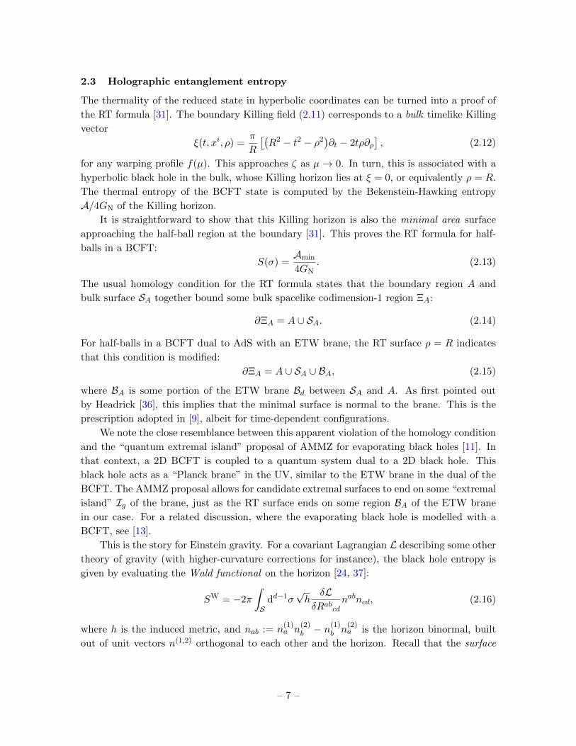
2.3 Holographic entanglement entropy
The thermality of the reduced state in hyperbolic coordinates can be turned into a proof of
the RT formula [31]. The boundary Killing field (2.11) corresponds to a bulk timelike Killing
vector
ξ(t, xi, ρ) =π
R
[(R2 − t2 − ρ2
)∂t − 2tρ∂ρ
], (2.12)
for any warping profile f(µ). This approaches ζ as µ→ 0. In turn, this is associated with a
hyperbolic black hole in the bulk, whose Killing horizon lies at ξ = 0, or equivalently ρ = R.
The thermal entropy of the BCFT state is computed by the Bekenstein-Hawking entropy
A/4GN of the Killing horizon.
It is straightforward to show that this Killing horizon is also the minimal area surface
approaching the half-ball region at the boundary [31]. This proves the RT formula for half-
balls in a BCFT:
S(σ) =Amin
4GN. (2.13)
The usual homology condition for the RT formula states that the boundary region A and
bulk surface SA together bound some bulk spacelike codimension-1 region ΞA:
∂ΞA = A ∪ SA. (2.14)
For half-balls in a BCFT dual to AdS with an ETW brane, the RT surface ρ = R indicates
that this condition is modified:
∂ΞA = A ∪ SA ∪ BA, (2.15)
where BA is some portion of the ETW brane Bd between SA and A. As first pointed out
by Headrick [36], this implies that the minimal surface is normal to the brane. This is the
prescription adopted in [9], albeit for time-dependent configurations.
We note the close resemblance between this apparent violation of the homology condition
and the “quantum extremal island” proposal of AMMZ for evaporating black holes [11]. In
that context, a 2D BCFT is coupled to a quantum system dual to a 2D black hole. This
black hole acts as a “Planck brane” in the UV, similar to the ETW brane in the dual of the
BCFT. The AMMZ proposal allows for candidate extremal surfaces to end on some “extremal
island” Ig of the brane, just as the RT surface ends on some region BA of the ETW brane
in our case. For a related discussion, where the evaporating black hole is modelled with a
BCFT, see [13].
This is the story for Einstein gravity. For a covariant Lagrangian L describing some other
theory of gravity (with higher-curvature corrections for instance), the black hole entropy is
given by evaluating the Wald functional on the horizon [24, 37]:
SW = −2π
∫S
dd−1σ√h
δLδRabcd
nabncd, (2.16)
where h is the induced metric, and nab := n(1)a n
(2)b − n
(1)b n
(2)a is the horizon binormal, built
out of unit vectors n(1,2) orthogonal to each other and the horizon. Recall that the surface
– 7 –

Figure 2. Left. The bulk causal domain D[B+] (green), cut away to reveal the boundary causal
domain D[B+] (red). The minimal surface is purple. Right. The Penrose diagram for the hyperbolic
black hole. The minimal surface and bifurcation surface (purple) coincide.
gravity κ of a black hole, with Killing horizon generated by ξ, is defined by
∇[cξd] = κncd. (2.17)
The Killing vector ξ in (2.12) is normalized such that κ = 2π.
Consider a perturbation to the state of our theory which corresponds to a perturbation
of the metric in the bulk, g → g + δg. To first order in δg, the change in the entanglement
entropy for a half-ball B+ is given by the change in (2.16):
δSB+ = δSWB+ , (2.18)
where SW is the Wald functional evaluated on the unperturbed minimal surface SB+ .6 The
modular Hamiltonian (2.10) involves an integral over the boundary stress-energy, so under a
change of state dual to the change of metric,
δ〈HB+〉 =
∫Σ+
dΣµζνδ〈Tµν〉. (2.19)
Near the boundary, and away from the brane, we can use the usual Fefferman-Graham coordi-
nate system with coordinate z, and expand δgab := zd−2h(d)ab +O(zd−1). The variation in CFT
stress-tensor expectation is proportional to this leading piece projected onto the boundary,
δ〈Tµν〉 = Ch(d)µν , and hence
δ〈HB+〉 = C
∫Σ+
dΣµζνh(d)µν . (2.20)
This is well-known for Einstein gravity, but holds more generally [20]. Even with the iden-
tifications (2.18–2.20), the first law (2.9) need not be satisfied for arbitrary δg. The main
6Evaluating on the perturbed surface produces second-order corrections. Moreover, it is known that
the Wald functional does not produce the entanglement entropy of an arbitrary boundary region in higher-
derivative gravity due to differences in the universal terms [38]. These corrections are quadratic in the extrinsic
curvature of SA, and hence vanish for the Killing horizon associated with the half-ball A = B+.
– 8 –

Figure 3. Left. The first law from Stokes theorem in AdS/CFT. Right. For AdS/BCFT, the first law
requires that the contribution from the brane vanishes.
result of [20] is that the first law (2.9) for ball-shaped regions B in the CFT implies that
perturbations around the AdS vacuum obey linearized equations of motion. Perhaps this is
unsurprising when we have defined both sides holographically in terms of the Wald entropy.
But the energy variation only knows about the metric near the boundary, while the entropy
variation knows about the deep bulk. We require a condition on δg to ensure these two
variations agree.
Suppose there exists a (d− 1)-form χB with the properties that∫BχB = δ〈HB〉,
∫SBχB = δSB, (2.21)
where SB is the extremal surface associated with B. In addition, suppose the (spacetime)
exterior derivative of χ vanishes when δg is on-shell, i.e., dχ ∝ δE, where δE are the linearized
equations of motion. Then for ΞB in (2.14), the first law follows from Stokes theorem:
0 =
∫ΞB
dχ =
∫B−SB
χ = δSB − δ〈HB〉. (2.22)
We defer the definition and detailed treatment of χB to the next section.
In the BCFT, the homology condition is modified to (2.15). Even if we can construct a
(d− 1)-form which is exact on-shell, the integral (2.22) will become∫BB+
χB+ = δSB+ − δ〈HB+〉. (2.23)
Since the energy (calculated from the half-ball modular Hamiltonian) and entropy (calculated
from the bulk black hole horizon) are fixed, the first law requires that the integral over the
brane vanishes. We will see that this enforces a Neumann condition in Einstein gravity. This
resembles the logic of gravitation from entanglement in CFTs: the first law places a constraint
on integrated metric fluctuations, which in turn is equivalent to local linearized dynamics.
3 Covariant phase space formalism
According to Noether’s theorem, every continuous symmetry yields a conserved current, with
an associated charge generating the symmetry transformation via the Poisson bracket (classi-
cal mechanics) or commutator (quantum mechanics). In the Hamiltonian formalism, defining
– 9 –

these brackets breaks spacetime covariance by selecting a preferred time-slicing. For diffeo-
morphism invariant theories, the covariant phase space formalism [22–26] provides an alterna-
tive. This endows the space of solutions with a natural symplectic form Ω [22], whose inverse
Ω−1 is the Poisson bracket in classical theories, and the commutator in quantum theories.
Let P be our phase space of solutions, which is a subset of all possible field configurations.
Suppose that P is also equipped with a symplectic form: a closed, nondegenerate 2-form
Ω ∈ Λ2(P). Closure means δΩ = 0, where δ is the exterior derivative in the space of field
configurations, while the nondegeneracy condition is
Ω(X,Y ) = 0 for all Y =⇒ X = 0. (3.1)
This induces a map from tangent vectors on P to one-forms:
X 7→ ωX := Ω(·, X) = −ιXΩ, (3.2)
where the minus sign arises from anticommuting X into the second slot. By nondegeneracy,
this map is invertible, with Ω−1(·, ωX) = X.
Consider a continuous symmetry along a flow ξ in spacetime, generated by a charge
Hξ : P → R. A familiar example is time translation and the Hamiltonian H. To define the
action on phase space, we first construct the (phase space) vector field dual to δHξ:
Ξ := Ω−1(·, δHξ), δHξ = Ω(·,Ξ). (3.3)
For any function f : P → R, the infinitesimal variation is then
δξf := ιΞδf = Ω−1(δf, δHξ). (3.4)
This is Hamilton’s equation f = f,H in covariant phase space language. We should caution
the reader that δf is a one-form on configuration space, while δξf maps points in phase space
(solutions to the equations of motion) to functions on spacetime (variations of f). For a
general configuration-space differential form ω, we define the variation under ξ using the Lie
derivative:
δξω := LΞω. (3.5)
This agrees with (3.4) for a 0-form f . Our goal in this section is to find an expression for the
generator of infinitesimal transformations, δHξ, in the presence of a boundary.
3.1 The symplectic form
The boundary of our manifold Md+1 has a region asymptotic to the BCFT as well as an ETW
brane, with ∂Md+1 = Hd ∪ Bd. Even in the vacuum boundary state |B〉, bulk fields can be
switched on, which can be holographically modelled with bulk field sources on the brane [7].
We therefore consider the more general scenario of a manifold M with boundary
∂Md+1 = Σ+ ∪ Σ− ∪ Γ, N ⊂ Γ, (3.6)
– 10 –
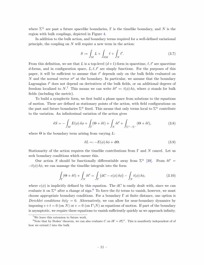
where Σ± are past a future spacelike boundaries, Γ is the timelike boundary, and N is the
region with bulk couplings, depicted in Figure 4.
In addition to the bulk action, and boundary terms required for a well-defined variational
principle, the coupling on N will require a new term in the action:
S :=
∫ML+
∫∂M
`+
∫N`′. (3.7)
From this definition, we see that L is a top-level (d+ 1)-form in spacetime, `, `′ are spacetime
d-forms, and in configuration space, L, `, `′ are simply functions. For the purposes of this
paper, it will be sufficient to assume that `′ depends only on the bulk fields evaluated on
N and the normal vector nµ at the boundary. In particular, we assume that the boundary
Lagrangian `′ does not depend on derivatives of the bulk fields, or on additional degrees of
freedom localized to N .7 This means we can write δ`′ =: t(φ) δφ, where φ stands for bulk
fields (including the metric).
To build a symplectic form, we first build a phase space from solutions to the equations
of motion. These are defined as stationary points of the action, with field configurations on
the past and future boundaries Σ± fixed. This means that only terms local to Σ± contribute
to the variation. An infinitesimal variation of the action gives
δS = −∫ME(φ) δφ+
∫Γ(Θ + δ`) +
∫Nδ`′ +
∫Σ+−Σ−
(Θ + δ`), (3.8)
where Θ is the boundary term arising from varying L:
δL =: −E(φ) δφ+ dΘ. (3.9)
Stationarity of the action requires the timelike contributions from Γ and N cancel. Let us
seek boundary conditions which ensure this.
Our action S should be functionally differentiable away from Σ± [39]. From δ`′ =
−t(φ) δφ, we can massage the timelike integrals into the form∫Γ(Θ + δ`) +
∫Nδ`′ =
∫Γ
(dC − e(φ) δφ
)−∫Nt(φ) δφ, (3.10)
where e(φ) is implicitly defined by this equation. The dC is easily dealt with, since we can
evaluate it on Σ± after a change of sign.8 To force the δφ terms to vanish, however, we must
choose appropriate boundary conditions. For a boundary Γ at finite distance, one option is
Dirichlet conditions δφ|Γ = 0. Alternatively, we can allow for near-boundary dynamics by
imposing e+ t = 0 (on N) or e = 0 (on Γ\N) as equations of motion. If part of the boundary
is asymptotic, we require these equations to vanish sufficiently quickly as we approach infinity.
7We leave this extension to future work.8Note that by Stokes’ theorem, we can also evaluate C on ∂Γ = ∂Σ±. This is manifestly independent of of
how we extend ` into the bulk.
– 11 –

Figure 4. A manifold M with boundary ∂M = Σ+ ∪ Σ− ∪ Γ, and timelike region N ⊂ Γ coupling
to bulk fields.
Suppose we have chosen boundary conditions ensuring the Γ\N term vanishes, for in-
stance, the canonical choice of Dirichlet conditions on the AdS boundary, while not making
any statment for the situation on the ETW brane. In this case, the general variation of S
takes the form
δS = −∫ME(φ) δφ−
∫N
(e(φ) + t(φ)
)δφ+
∫Σ+−Σ−
(Θ + δ`− dC). (3.11)
The pre-symplectic potential ω is the exterior derivative of the last integrand:
ω := δ(Θ + δ`− dC) = δ (Θ− dC) , (3.12)
since δ2` = 0. The pre-symplectic form Ω is the integral of ω over some Cauchy slice Σ:
Ω :=
∫Σω. (3.13)
In order to obtain phase space proper, we must quotient out the zero modes, defining P :=
P/G, on which Ω lifts to a genuine symplectic form Ω [26].
3.2 The generator of infinitesimal diffeomorphisms
We now consider theories which are invariant under arbitrary diffeomorphisms preserving the
boundary conditions. The symmetry acts on configuration space according to (3.4) or (3.5).
In order for the theory to be covariant, the spacetime variation under a diffeomorphism ξ
should induce the corresponding field variation:
δξL = LξL. (3.14)
In general, a configuration space form ω transforms covariantly if the action on the fields,
induced by the flow Ξ, agrees with the full spacetime variation under ξ:
δξω = Lξω. (3.15)
– 12 –

By a theorem of Iyer and Wald [24], if L is covariant, then the integration by parts used to
define Θ can be performed covariantly, and hence Θ can be taken to be covariant.
By Cartan’s magic formula
LXω = X · dω + d(X · ω), (3.16)
the Lie derivative of L reduces to an exterior derivative
LξL = ξ · dL+ d(ξ · L) = d(ξ · L), (3.17)
where dL = 0 since L is a top-level spacetime form. Similar statements hold for the d-forms
`, `′ on ∂M . The action (3.7) transforms as
δξS =
∫MLξL+
∫∂MLξ`+
∫NLξ`′ =
∫∂M
ξ · L+
∫∂N
ξ · `′, (3.18)
using Stokes’ theorem and ∂2Md+1 = 0. Equating this to an insertion ιΞδS in the general
field variation (3.8), we find that for a diffeomorphism-covariant theory,∫ME(φ) δξφ =
∫Nδξ`′ +
∫∂M
δξ`+
∫∂M
ιΞΘ−∫∂M
ξ · L−∫∂N
ξ · `′
=
∫∂M
(ιΞΘ− ξ · L). (3.19)
The contributions from `′ cancel, while the ` integral vanishes. If the equations of motion
hold, the left hand side of (3.19) is zero, suggesting we define the Noether current
Jξ := ιΞΘ− ξ · L. (3.20)
A quick calculation using (3.9), (3.17), and dδ = δd shows that, for a covariant Lagrangian,
dJξ = −LξL+ δξL+ E(φ)δξφ = E(φ)δξφ,
so Jξ is conserved on-shell. When the result is true for arbitrary diffeomorphisms ξ, the
on-shell conservation dJξ = 0 implies [40] the existence of a (d − 2)-form Noether “charge”
Qξ, defined by
Jξ = dQξ. (3.21)
The derivation of Jξ depends only on bulk equations of motion, and is insensitive to the
tension of the brane. The “charge” Qξ arises due to bulk diffeomorphism invariance, which
is also independent of boundary conditions.
We can now derive the infinitesimal generator δHξ. First, we take the exterior derivative
of Jξ in configuration space, using (3.12), Cartan’s formula (3.16) for both δ and d, (3.9), the
covariance of Θ, and the fact that δ commutes with spacetime insertions:
δJξ = −ξ · δL+ δ(ιΞΘ)
= ξ · (E(φ)δφ− dΘ)− ιΞδΘ + LΞΘ
= ξ · E(φ)δφ− LξΘ + LΞΘ + d(ξ ·Θ)− ιΞδΘ= ξ · E(φ)δφ+ d(ξ ·Θ)− ιΞω − ιΞδdC. (3.22)
– 13 –
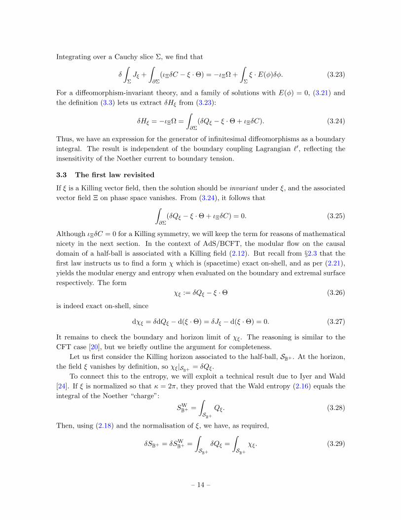
Integrating over a Cauchy slice Σ, we find that
δ
∫ΣJξ +
∫∂Σ
(ιΞδC − ξ ·Θ) = −ιΞΩ +
∫Σξ · E(φ)δφ. (3.23)
For a diffeomorphism-invariant theory, and a family of solutions with E(φ) = 0, (3.21) and
the definition (3.3) lets us extract δHξ from (3.23):
δHξ = −ιΞΩ =
∫∂Σ
(δQξ − ξ ·Θ + ιΞδC). (3.24)
Thus, we have an expression for the generator of infinitesimal diffeomorphisms as a boundary
integral. The result is independent of the boundary coupling Lagrangian `′, reflecting the
insensitivity of the Noether current to boundary tension.
3.3 The first law revisited
If ξ is a Killing vector field, then the solution should be invariant under ξ, and the associated
vector field Ξ on phase space vanishes. From (3.24), it follows that∫∂Σ
(δQξ − ξ ·Θ + ιΞδC) = 0. (3.25)
Although ιΞδC = 0 for a Killing symmetry, we will keep the term for reasons of mathematical
nicety in the next section. In the context of AdS/BCFT, the modular flow on the causal
domain of a half-ball is associated with a Killing field (2.12). But recall from §2.3 that the
first law instructs us to find a form χ which is (spacetime) exact on-shell, and as per (2.21),
yields the modular energy and entropy when evaluated on the boundary and extremal surface
respectively. The form
χξ := δQξ − ξ ·Θ (3.26)
is indeed exact on-shell, since
dχξ = δdQξ − d(ξ ·Θ) = δJξ − d(ξ ·Θ) = 0. (3.27)
It remains to check the boundary and horizon limit of χξ. The reasoning is similar to the
CFT case [20], but we briefly outline the argument for completeness.
Let us first consider the Killing horizon associated to the half-ball, SB+ . At the horizon,
the field ξ vanishes by definition, so χξ|SB+ = δQξ.
To connect this to the entropy, we will exploit a technical result due to Iyer and Wald
[24]. If ξ is normalized so that κ = 2π, they proved that the Wald entropy (2.16) equals the
integral of the Noether “charge”:
SWB+ =
∫SB+
Qξ. (3.28)
Then, using (2.18) and the normalisation of ξ, we have, as required,
δSB+ = δSWB+ =
∫SB+
δQξ =
∫SB+
χξ. (3.29)
– 14 –

The horizon integral gives the variation in entropy.
We now consider the boundary integral over the half-ball B+. It can be shown [20] that
this integral reduces to (2.20), and hence
δ〈HB+〉 =
∫B+
χξ =
∫B+
(δQξ − ζ ·Θ
), (3.30)
using ξ → ζ at the boundary. It follows that, when linearized perturbations are on-shell in
the bulk with E(φ) = 0, we have
δS[ξ]− δ〈HB+〉 =
∫BB+
χξ.
Thus, the first law δS = δ〈H〉 implies that the brane contribution vanishes:∫BB+
χξ = 0. (3.31)
This statement holds for the broad class of covariant bulk Lagrangians and bulk couplings
we are considering.
In the preceding argument, we have implicitly assumed that there is no additional
delta-localized stress-energy source (or more precisely, variation thereof) on the boundary
of the CFT. Since we consider linearized metric fluctuations only, and do not introduce any
boundary-localized fields, this seems like a reasonable assumption.
Furthermore, as the authors of [41] have argued, one should expect that in a quantum
theory, the non-conservation of a boundary stress-energy tensor “thickens” boundary degrees
of freedom, such that the theory contains only one single stress energy tensor without delta-
function support on the boundary. This operator is conserved and the normal-transverse
component to the brane, Tna|B = 0 vanishes. The non-trivial normal-normal component of
the stress-energy tensor becomes the displacement operator [42] as we approach the boundary.
However, this component does not appear in the present discussion.
It might still be that the expectation value of the CFT stress-energy tensor contains
delta-function terms localized to the boundary. In fact, generally such terms appear in the
Weyl anomaly of a BCFT. However, since we assume a flat boundary such terms to not
contribute and by energy-momentum conservation, localized stress-energy at the boundary
does not require any other treatment than localized stress-energy at any other point.
In light of recent progress on the black hole information paradox [10], it would interesting
to understand how this relates to toy models where quantum mechanical degrees of freedom
dual to gravity are localized on the boundary of the CFT. We leave this to future work.
4 Equations of motion from the first law
The integrals along the extremal surface and boundary, discussed in the previous section,
give the variation in entanglement entropy and modular energy appearing on either side of
– 15 –

the first law. Restricting to metric perturbations which satisfy the first law implies that the
brane contribution (3.31) vanishes. In principle, this can be used to reverse engineer linearized
equations of motion for the brane in any covariant theory of gravity. We will consider the
familiar case of Einstein gravity as a proof of concept.
4.1 Generator at the ETW brane
In coordinates, the first two terms of (3.25) read
(δQξ − ξ ·Θ)αβ··· =εαβ···γδ16πGN
(δgγλ∇λξδ −
1
2δgλλ∇γξδ − ξλ∇γδgδλ
− gγλξδ∇κδgλκ + gγλξδ∇λδgκκ),
(4.1)
where the · · · stand for additional transverse directions. Since we are integrating over a
codimension-2 region, we can choose a two-dimensional basis of vectors normal to the path
of integration, with γ the index parallel to the brane and δ normal to it. We will calculate
the expression piece by piece.
• Parallel terms. First, we consider terms with index γ. Using this, along with the fact
that at the brane, ξµnµ = 0 and hµνξν = ξµ, we find
(δQξ − ξ ·Θ)αβ···(1)⊃
εαβ···γδ16πGN
nδhγµξν(− δgλµKλν + δgµλn
λnαnβ∇αξβ
+1
2δgλλKµν − nλ∇µδgνλ
),
(4.2)
where Kµν is the extrinsic curvature. To streamline the notation, we will use a SVT–like
decomposition of the metric fluctuations:
γµν := h αµ δgαβh
βν (4.3)
Aµ := h αµ δgαβn
β (4.4)
φ := nαδgαβnβ. (4.5)
Reorganising all of (4.2) into these terms, we arrive at
(δQξ − ξ ·Θ)αβ···(1)⊃
εαβ···γδ16πGN
nδhγµξν
[− γαµKαν +
1
2(φ+ γλλ)Kµν − nλ∇µδgνλ
]+εαβ···γδ16πGN
nδhγµ(Aµn
αnβ∇αξβ).
(4.6)
• Normal terms. We next consider terms which arise from exchanging γ and δ in (4.1).
We can write this as
(δQξ − ξ ·Θ)αβ···(2)⊃
εαβ···γδ16πGN
nδhγµξν
[hµνn
ρhαβ(∇αδgρβ −∇ρgαβ) + nρ∇ρδgµν
]
+εαβ···γδ16πGN
nδhγµ
[1
2(γλλ − φ)nρ∇ρξµ −AaDaξµ
],
(4.7)
– 16 –

and therefore find
(δQξ − ξ ·Θ)αβ···(2)⊃
εαβ···γδ16πGN
nδhγµξν
[hµνh
αβnρ(∇αδgρβ +∇βδgρα −∇ρδgαβ)
+nρ∇ρδgµν +1
2φKµν −
1
2γλλKµν + hµνK
αβγαβ − hµνKφ
]
−nδhγµ[
1
2φnρ∂ρξµ −
1
2γλλn
ρ∂ρξµ +Da(Aaξµ)
].
(4.8)
Above, D denotes the covariant derivative on the brane, and we have used that
h α2α1
. . . h αnαn−1∇α2Tα4...αn = h α2
α1. . . h αn
αn−1Dα2Tα4...αn
if T is transverse to the brane.
• A convenient zero. Finally, we consider ιΞδC. This vanishes for a Killing field
ξ. However, if we evaluate for an arbitrary ξ, we obtain 0 in a convenient form that
simplifies the contributions above.
Recall that δC is a spacetime (d − 1)-form and a phase-space one-form. In our
coordinates, and again using our convention that γ is the coordinate direction parallel
to the brane but orthogonal to the direction of integration, it reads [26]
δC = δ2(√−hhγνδ1gνµn
µ), (4.9)
where we have to antisymmetrize δ1 and δ2. In more detail:
δ2(√−hhγνδ1gνµn
µ) =√−hhγν
[1
2hαβδ2gαβδ1gνµn
µ − δ2gνµhµαδ1gαβn
β
− hµαδ2gαβnβδ1gνµ −
1
2nαδ2gαβn
βδ1gνµnµ
]− (1↔ 2).
(4.10)
Due to this antisymmetrization, the second and third terms cancel. Antisymmetrizing,
calculating the interior product ιΞδC, and replacing δ2gµν by Lξgµν , after some algebra
we obtain
ιΞδC =√−hhγµ
[Aµ(Dαξα − nαnβ∇αξβ) +
1
2(γαα − φ)(ξνKνµ − nν∇νξµ)
]. (4.11)
• The final expression. To obtain the final expression, we add (4.6), (4.8), and (4.11):
(χξ)αβ··· =εαβ···γδ16πGN
nδhγµξν[hµνn
ρ(hαβ − hαµhβν )(∇αδgρβ −∇ρδgαβ)
−γαµKαν + γλλKµν
]+εαβ···γδ16πGN
nδhγµ(−AaDaξµ
)+√−hhcµ
(AµDαξα
).
(4.12)
– 17 –

• The Neumann condition. This seems unwieldy, but is directly related to the Neu-
mann condition on the brane. Using the identity
0 = −hαµhβνnρ∇βδgρα +DνAµ + φKµν −Kλν γλµ, (4.13)
we can rewrite (4.12) as
(χξ)αβ··· =εαβ···γδ16πGN
nδhγµξν[nρ(hµνh
αβ − hαµhβν )(∇αδgρβ +∇βδgρα −∇ρδgαβ)
+φ(Kµν − hµνK) + hµνKαβγαβ +Kµνγ
λλ − 2γκµKκν
]−nδhγµDκ(Aκξµ − ξκAµ).
(4.14)
If the background obeys the brane equation of motion (2.6), it follows that
hµνKαβγαβ + γαβh
αβKνµ − 2γκµKκν = 2[hµνK
αβ − hαµhβν (K + T )]γαβ. (4.15)
This turns equation (4.14) into an expression proportional to a linearized Neumann
condition, plus some additional terms depending on Aµ. Luckily, we can eliminate
these by choosing normal coordinates close to the brane. In these coordinates, we have
(χξ)αβ··· =εαβ···γδ16πGN
nδhγµξνδNµν , (4.16)
where the Neumann condition at first order (derived in Appendix B) is:
0 = δNµν := nρ(hµνhαβ − hαµhβν )(∇αδgρβ +∇βδgρα −∇ρδgαβ)
+(Kµν − hµνK)φ+ 2[hµνK
αβ − hαµhβν (K + T )]γαβ.
(4.17)
4.2 Local equations of motion
Combining the explicit expression (4.16), and the first law in the form (3.31), we learn that∫BAχA ∝
∫BAhγµξνδNµνnδ = 0 (4.18)
for any boundary-centered half-ball A. We will see that this set of global conditions implies
the local condition δNµν = 0 everywhere on the brane. This is analogous to [20], where the
first law gives global constraints equivalent to local, linearized bulk equations of motion.
First, we can use the trick in [20] to trade global constraints on χA, which depends on
boundary region A, for global constraints on δNµν . Choosing our Cauchy slice to intersect
t = 0 on the brane (Figure 5), and applying the differential operator R−1∂RR to (4.18),
produces two terms: an integral of χA localised to ρ = R, where the Killing vector ξA is zero
by definition, and another term involving the derivative of the Killing vector. Noting that
both hγµ and ξνA project onto the timelike direction, we find∫BAδNtt = 0. (4.19)
– 18 –

Figure 5. Left: The Cauchy slice, with t = 0, used to show that the integral of δNtt on BA vanishes.
Right: The Cauchy slice, with t = α(R− r), used to show that the integral of δNtρ on BA vanishes.
For the standard t = 0 Cauchy slice, the regions BA are hemisphere-shaped, and we can
invoke the argument from Appendix A of [20] to conclude that9
δNtt = 0. (4.21)
By boosting along the BCFT boundary, we then find that δNuu = uµuνδNµν = 0 vanishes
for any timelike vector u along this boundary, implying that δNab = 0 for all a, b parallel to
this boundary. We still need to show that the components of δN in the z-direction (or
equivalently ρ) vanish. This is achieved by choosing our Cauchy slices to lie at t = α(R− r),with 0 ≤ α < 1. In our case, this is in fact possible by conservation of the stress-energy
tensor, even at the boundary. Using this slicing, and applying ∂RR to (4.18), we arrive at10∫BA[2R(1− α2) + 2rα2]∂t − 2αρ∂ρµδNµν∂r + α∂ρν = 0. (4.22)
After taking the limit α→ 0, and applying another derivative with respect to R, we find∫BAδNtρ = 0. (4.23)
By the same argument as above, δNtρ = 0 everywhere on the brane. Since the other com-
ponents vanish, we immediately have δNtz = 0. Substituting into (4.22), we deduce that
9One way to see this is by taking derivatives of (4.19) with respect to the variables parametrizing BA,
namely its radius R and center xi0. Applying ∂R or ∂xi0respectively gives∫
∂SA∩∂BAδNtt =
∫∂SA∩∂BA
xiδNtt = 0. (4.20)
We can repeat this process, substituting the integrands of (4.20) into (4.19), to conclude that the overlap
integral of δNtt with an arbitrary polynomial in xi vanishes. Since δNtt is continuous, it can be approximated
to arbitrary precision by such a polynomial, and the vanishing overlaps imply δNtt = 0 on ∂SA ∩ ∂BA, since
the integral of (δNtt)2 vanishes to arbitrary precision. These semi-circles ∂SA ∩ ∂BA cover the brane, so we
must have δNtt = 0 everywhere.10Here we omit and additional factor of 1/
√1− α2 that can be divided out.
– 19 –

δNρρ ∝ δNzz vanishes everywhere on the brane. Assembling the components, we find the
local equation of motion δNµν = 0 everywhere on the brane. If we exclude the trivial case of
Dirichlet conditions, which set all metric fluctuations close to the brane to zero, we conclude
that metric fluctuations must obey Neumann boundary conditions.
5 Discussion
In this note, we have probed the consequences of the first law of entanglement for boundary
CFTs dual to AdS cut off by an ETW brane. We find that, for a broad class of gravita-
tional Lagrangians, the first law implies that bulk Noether charges associated with boundary-
centered half-balls must vanish when integrated over associated regions of the brane. For the
specific case of Einstein gravity in the bulk, and perturbations to a brane of constant curva-
ture, this vanishing implies local, linearized equations of motion δNµν = 0, where Nµν = 0 is
the background Neumann condition. In other words: if the brane obeys a background Neu-
mann condition, the first law implies that non-vanishing metric fluctuations obey a linearized
Neumann condition at the brane.
Our main tool is that for half-ball shaped regions in the BCFT, both the entanglement
entropy and the vacuum modular Hamiltonian are known. This closely parallels the logic
of [20], where a background obeying Einstein’s equations (or some more general covariant
equations of motion) are forced to obey linearized equations by the first law. Our method
should generalize to give local, linearized equations for perturbations to the brane in more
general theories of gravity.
We have focused on pure gravity, where the only relevant feature of the boundary state
is its tension, sourcing the identity sector of the BCFT. Although warping partially captures
the effect of (unperturbed) background fields, it would be interesting to perturb light fields in
the bulk and determine the restrictions arising from the corresponding statement of the first
law [43]. We expect to find that these light bulk fields obey linearized equations sourced by
the ETW brane. Using these methods, it may even be possible to map a consistent boundary
state, satisfying some explicit holographic restrictions, to a solution of bulk equations in the
presence of a localized source. This would be the equivalent to [44] for a BCFT.
Similarly, one might envision additional fields or dynamical gravity on the brane itself.
This presumably requires an even more careful treatment of the boundary contributions to
the Noether charge and the effects of additional degrees of freedom localized to the BCFT
boundary. While it did not seem to play an important role in our discussion, a Hayward term
might need to be included [45] (for recent work, see e.g. [46]). A thorough analysis could lead
to an extended holographic dictionary between bulk modes and fields localized on the brane.
This note has shown that quantum information-theoretic considerations, successfully ap-
plied in AdS/CFT to constrain bulk dynamics [20] and semiclassical states [47], can also be
used to constrain the dynamics of holographic BCFTs. It would be interesting to consider
holographic constraints on excited states of BCFTs, e.g., positive energy theorems in the bulk
– 20 –

[47, 48] , but we leave this question, and the sundry extensions mentioned above, to future
work.
Acknowledgements
We are thankful to Jamie Sully and Mark Van Raamsdonk for useful discussions. MR and
SC are supported by a Discovery grant from NSERC. DN is partially supported by the
University of British Columbia through a Four Year Fellowship and the Simons Foundation
through an It from Qubit Postdoctoral Fellowship. DW is supported by an International
Doctoral Fellowship from the University of British Columbia. Research at Perimeter Institute
is supported in part by the Government of Canada through the Department of Innovation,
Science and Economic Development Canada and by the Province of Ontario through the
Ministry of Economic Development, Job Creation and Trade.
A Useful formulae and conventions
We can decompose the metric close to the brane into two parts:
gµν = nµnν + hµν , (A.1)
where nµ is the normal vector to the boundary with n · n = 1 and hµν is orthogonal to
nµ, nµhµν = 0. Since the covariant derivative is metric compatible, we have that ∇α(nµnν +
hµν) = 0. Contracting this equation with nµ and hβν and also projecting α onto the transverse
space we obtain the useful identity
Kαβ = −hβνnµ∇αhµν . (A.2)
Finally, we need some standard results for the variation of h and n under perturbations to g:
√−h =
1
2
√−hhαβδgαβ (A.3)
δ(hcν) = −hcαδgαβhβν (A.4)
δ(nµ) = −gµρδgρνnν +1
2nµnαδgαβn
β. (A.5)
B The Neumann condition at first order
In the path integral, we restrict to configurations obeying the modified Neumann condition.
In particular, this means that perturbations satisfy
δ(Kab − habK) = Tδhab. (B.1)
– 21 –
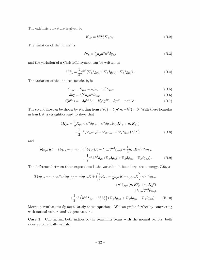
The extrinsic curvature is given by
Kµν = hαµhβν∇αnβ. (B.2)
The variation of the normal is
δnµ =1
2nµn
αnβδgαβ (B.3)
and the variation of a Christoffel symbol can be written as
δΓαµν =1
2gαβ (∇µδgβν +∇νδgβµ −∇βδgµν) . (B.4)
The variation of the induced metric, h, is
δhµν = δgµν − nµnνnαnβδgαβ (B.5)
δhλµ = hλνnµnαδgαν (B.6)
δ(hµν) = −δgµαhνα − hµβδg
βν + δgµν − nµnνφ. (B.7)
The second line can be shown by starting from δ(δµν ) = δ(nµnν−hµν ) = 0. With these formulas
in hand, it is straightforward to show that
δKµν =1
2Kµνn
ρnσδgρσ + nσδgρσ(nµKρν + nνK
ρµ )
−1
2nρ (∇αδgρβ +∇βδgρα −∇ρδgαβ)hαµh
βν (B.8)
and
δ(hµνK) = (δgµν − nµnνnαnβδgαβ)K − hµνKαβδgαβ +1
2hµνKn
ρnσδgρσ
−1
2nρhαβhµν (∇αδgρβ +∇βδgρα −∇ρδgαβ) . (B.9)
The difference between these expressions is the variation in boundary stress-energy, Tδhab:
T (δgµν − nµnνnαnβδgαβ) = −δgµνK +
(1
2Kµν −
1
2hµνK + nµnνK
)nρnσδgρσ
+nσδgρσ(nµKρν + nνK
ρµ )
+hµνKαβδgαβ
+1
2nρ(hαβhµν − hαµhβν
)(∇αδgρβ +∇βδgρα −∇ρδgαβ) . (B.10)
Metric perturbations δg must satisfy these equations. We can probe further by contracting
with normal vectors and tangent vectors.
Case 1. Contracting both indices of the remaining terms with the normal vectors, both
sides automatically vanish.
– 22 –
Case 2. Contracting one index with the normal, and the other with the projector onto the
tangent space, we obtain
0 = (Kµρ − hµρK − hµρT )hνρδgνσnσ. (B.11)
This vanishes by the boundary condition.
Case 3. Finally, we consider projecting δg onto the tangent space. First, define
nρnσδgρσ = δgnn, hαµhβν δgαβ = δg⊥µν . (B.12)
Contracting both with hµν , we find
0 =1
2(Kµν − hµνK) δgnn + (hµνK
αβ − hαµhβν (K + T ))δg⊥αβ
+1
2nρ(hαβhµν − hαµhβν
)(∇αδgρβ +∇βδgρα −∇ρδgαβ) . (B.13)
This can be shortened using the variation formula for the Christoffel symbol:
0 =1
2(Kµν − hµνK) δgnn + (hµνK
αβ − hαµhβν (K + T ))δg⊥αβ + nρ
(hαβhµν − hαµhβν
)δΓραβ.
(B.14)
C Covariance and boundaries
At the heart of the covariant phase space formalism is the idea that a symmetry transformation
can be represented by an action on the fields. However, the presence of a boundary makes
the discussion slightly more difficult. In a fixed coordinate system, the action of a symmetry
on the fields cannot change the location of the boundary. Thus, in order for the action to be
invariant up to boundary terms, we require that the symmetry reduces to a symmetry of the
boundary at the boundary itself. For example, diffeomorphism symmetries must not change
the location to the boundary:
ξµnµ
∣∣∣∂M
= 0. (C.1)
One can introduce boundary quantities such as the normal vector in a coordinate-invariant
way by using a function f , defined in neighborhood of the boundary, which is smooth and
negative except at the boundary where it vanishes. One can then define a (space-like) by
normal vector
nµ :=∂µf√
∂αf∂βfgαβ. (C.2)
– 23 –

However, the Lie derivative implementing a general diffeomorphism does not act on f .
In order to preserve covariance, we therefore need the Lie derivative
Lξnµ = ξν∇νnµ + nν∇µξν (C.3)
to agree with the transformation under a symmetry of fields on the boundary:
δξnµ = nµnαnβ∇αξβ. (C.4)
Thus, the allowed diffeomorphisms obey
0 =(ξν∇νnµ + nν∇µξν − nµnαnβ∇αξβ
)∣∣∣∂M
. (C.5)
The normal component of this equation vanishes and the only non-trivial content is obtained
by projecting it onto the boundary,
0 = hαµξν∇νnµ + nνhαµ∇µξν . (C.6)
From this it follows that
0 = hαµ∂µ(ξνnν). (C.7)
In fact, we can even be less restrictive by requiring that the above equations do not hold in
a neighborhood around the boundary, but at the boundary to finite order in derivatives in
normal direction. For further discussion, see [26].
References
[1] J. L. Cardy, Conformal invariance and surface critical behavior, Nuclear Physics B 240 (1984)
514.
[2] J. M. Maldacena, The Large N Limit of Superconformal Field Theories and Supergravity,
International Journal of Theoretical Physics 38 (1997) 1113 [9711200].
[3] S. Gubser, I. Klebanov and A. Polyakov, Gauge theory correlators from non-critical string
theory, Physics Letters B 428 (1998) 105 [9802109].
[4] E. Witten, Anti de Sitter space and holography, Advances in Theoretical and Mathematical
Physics 2 (1998) 253 [9802150].
[5] A. Karch and L. Randall, Open and closed string interpretation of SUSY CFT’s on branes with
boundaries, Journal of High Energy Physics 2001 (2001) 063 [0105132].
[6] T. Takayanagi, Holographic Dual of a Boundary Conformal Field Theory, Physical Review
Letters 107 (2011) 101602 [1105.5165].
[7] M. Fujita, T. Takayanagi and E. Tonni, Aspects of AdS/BCFT, Journal of High Energy Physics
2011 (2011) 43 [1108.5152].
– 24 –

[8] A. Almheiri, T. Anous and A. Lewkowycz, Inside out: meet the operators inside the horizon.
On bulk reconstruction behind causal horizons, Journal of High Energy Physics 2018 (2018) 28
[1707.06622].
[9] S. Cooper, M. Rozali, B. Swingle, M. Van Raamsdonk, C. Waddell and D. Wakeham, Black
hole microstate cosmology, Journal of High Energy Physics 2019 (2019) 65 [1810.10601].
[10] A. Almheiri, R. Mahajan, J. Maldacena and Y. Zhao, The Page curve of Hawking radiation
from semiclassical geometry, 1908.10996.
[11] A. Almheiri, N. Engelhardt, D. Marolf and H. Maxfield, The entropy of bulk quantum fields and
the entanglement wedge of an evaporating black hole, 1905.08762.
[12] A. Almheiri, R. Mahajan and J. Maldacena, Islands outside the horizon, 1910.11077.
[13] M. Rozali, J. Sully, M. Van Raamsdonk, C. Waddell and D. Wakeham, Information radiation in
BCFT models of black holes, 1910.12836.
[14] M. Van Raamsdonk, Building up spacetime with quantum entanglement II: It from BC-bit,
1809.01197.
[15] T. Shimaji, T. Takayanagi and Z. Wei, Holographic quantum circuits from splitting/joining local
quenches, Journal of High Energy Physics 2019 (2019) 165 [1812.01176].
[16] S. Antonini and B. Swingle, Cosmology at the end of the world, 1907.06667.
[17] M. Chiodaroli, E. D’Hoker, Y. Guo and M. Gutperle, Exact half-BPS string-junction solutions
in six-dimensional supergravity, Journal of High Energy Physics 2011 (2011) 86 [1107.1722].
[18] M. Chiodaroli, E. D’Hoker and M. Gutperle, Holographic duals of boundary CFTs, Journal of
High Energy Physics 2012 (2012) 177 [1205.5303].
[19] M. Chiodaroli, E. D’Hoker and M. Gutperle, Simple holographic duals to boundary CFTs,
Journal of High Energy Physics 2012 (2012) 5 [1111.6912].
[20] T. Faulkner, M. Guica, T. Hartman, R. C. Myers and M. Van Raamsdonk, Gravitation from
entanglement in holographic CFTs, Journal of High Energy Physics 2014 (2014) 51
[1312.7856].
[21] T. Faulkner, F. M. Haehl, E. Hijano, O. Parrikar, C. Rabideau and M. Van Raamsdonk,
Nonlinear gravity from entanglement in conformal field theories, Journal of High Energy
Physics 2017 (2017) 57 [1705.03026].
[22] C. Crnkovic, Symplectic geometry of the convariant phase space, Classical and Quantum
Gravity 5 (1988) 1557.
[23] J. Lee and R. M. Wald, Local symmetries and constraints, Journal of Mathematical Physics 31
(1990) 725.
[24] V. Iyer and R. M. Wald, Some properties of the Noether charge and a proposal for dynamical
black hole entropy, Physical Review D 50 (1994) 846 [9403028].
[25] R. M. Wald and A. Zoupas, General definition of “conserved quantities” in general relativity
and other theories of gravity, Physical Review D 61 (2000) 084027 [9911095].
[26] D. Harlow and J.-q. Wu, Covariant phase space with boundaries, 1906.08616.
– 25 –

[27] A. Almheiri, X. Dong and D. Harlow, Bulk locality and quantum error correction in AdS/CFT,
Journal of High Energy Physics 2015 (2015) 163 [1411.7041].
[28] D. McAvity and H. Osborn, Conformal field theories near a boundary in general dimensions,
Nuclear Physics B 455 (1995) 522 [9505127].
[29] D. Bak, M. Gutperle and S. Hirano, A dilatonic deformation of AdS 5 and its field theory dual,
Journal of High Energy Physics 2003 (2003) 072 [0304129].
[30] M. Gutperle and J. Samani, Holographic renormalization group flows and boundary conformal
field theories, Physical Review D 86 (2012) 106007 [1207.7325].
[31] K. Jensen and A. O’Bannon, Holography, entanglement entropy, and conformal field theories
with boundaries or defects, Physical Review D 88 (2013) 106006 [1309.4523].
[32] E. Witten, Notes On Some Entanglement Properties Of Quantum Field Theory, Reviews of
Modern Physics 90 (2018) 045003 [1803.04993].
[33] H. Casini, E. Teste and G. Torroba, All the entropies on the light-cone, Journal of High Energy
Physics 2018 (2018) 5 [1802.04278].
[34] S. Ryu and T. Takayanagi, Aspects of holographic entanglement entropy, Journal of High
Energy Physics 2006 (2006) 045 [0605073].
[35] H. Casini, M. Huerta and R. C. Myers, Towards a derivation of holographic entanglement
entropy, Journal of High Energy Physics 2011 (2011) 36 [1102.0440].
[36] M. Headrick, General properties of holographic entanglement entropy, Journal of High Energy
Physics 2014 (2013) 85 [1312.6717].
[37] R. M. Wald, Black hole entropy is the Noether charge, Physical Review D 48 (1993) R3427
[9307038].
[38] X. Dong, Holographic entanglement entropy for general higher derivative gravity, Journal of
High Energy Physics 2014 (2014) 44 [1310.5713].
[39] T. Regge and C. Teitelboim, Role of surface integrals in the Hamiltonian formulation of general
relativity, Annals of Physics 88 (1974) 286.
[40] R. M. Wald, On identically closed forms locally constructed from a field, Journal of
Mathematical Physics 31 (1990) 2378.
[41] C. P. Herzog and K.-W. Huang, Boundary conformal field theory and a boundary central charge,
Journal of High Energy Physics 2017 (2017) 189 [1707.06224].
[42] C. Herzog, K.-W. Huang and K. Jensen, Displacement Operators and Constraints on Boundary
Central Charges, Physical Review Letters 120 (2018) 021601 [1709.07431].
[43] J. de Boer, F. M. Haehl, M. P. Heller and R. C. Myers, Entanglement, holography and causal
diamonds, Journal of High Energy Physics 2016 (2016) 162 [1606.03307].
[44] I. Heemskerk, J. Penedones, J. Polchinski and J. Sully, Holography from conformal field theory,
Journal of High Energy Physics 2009 (2009) 079 [0907.0151].
[45] G. Hayward, Gravitational action for spacetimes with nonsmooth boundaries, Physical Review D
47 (1993) 3275.
[46] T. Takayanagi and K. Tamaoka, Gravity Edges Modes and Hayward Term, 1912.01636.
– 26 –

[47] N. Lashkari, J. Lin, H. Ooguri, B. Stoica and M. Van Raamsdonk, Gravitational positive energy
theorems from information inequalities, Progress of Theoretical and Experimental Physics 2016
(2016) 12C109 [1605.01075].
[48] D. Neuenfeld, K. Saraswat and M. Van Raamsdonk, Positive gravitational subsystem energies
from CFT cone relative entropies, Journal of High Energy Physics 2018 (2018) 50
[1802.01585].
– 27 –